the Creative Commons Attribution 4.0 License.
the Creative Commons Attribution 4.0 License.
 | 11 Aug 2020
A spectral approach to estimating the timescale-dependent uncertainty of paleoclimate records – Part 1: Theoretical concept
Andrew M. Dolman
Thomas Laepple
Proxy records represent an invaluable source of information for reconstructing past climatic variations, but they are associated with considerable uncertainties. For a systematic quantification of these reconstruction errors, however, knowledge is required not only of their individual sources but also of their auto-correlation structure as this determines the timescale dependence of their magnitude, an issue that has been often ignored until now. Here a spectral approach to uncertainty analysis is provided for paleoclimate reconstructions obtained from single sediment proxy records. The formulation in the spectral domain rather than the time domain allows for an explicit demonstration and quantification of the timescale dependence that is inherent in any proxy-based reconstruction uncertainty. This study is published in two parts.
In this first part, the theoretical concept is presented, and analytic expressions are derived for the power spectral density of the reconstruction error of sediment proxy records. The underlying model takes into account the spectral structure of the climate signal, seasonal and orbital variations, bioturbation, sampling of a finite number of signal carriers, and uncorrelated measurement noise, and it includes the effects of spectral aliasing and leakage. The uncertainty estimation method, based upon this model, is illustrated by simple examples. In the second part of this study, published separately, the method is implemented in an application-oriented context, and more detailed examples are presented.
- Article
(1784 KB) - Full-text XML
- Companion paper
- BibTeX
- EndNote


The central issues of climate sciences include the estimation, understanding, and prediction of climatic variations across ranges of space and timescales that are relevant to the specific field of study. From an inductive perspective, such studies are necessarily based on observational data which the variability may be estimated from, whereas from a deductive perspective observational data are needed in the course of the validation of theories and models. For certain fields of study, instrumental or satellite data may provide a useful data source. Nonetheless, once processes are studied that involve climate states or variations at times before the instrumental era or that involve timescales longer than this, reconstructions obtained from paleoclimate proxies become indispensable. Such proxy records reveal imprints of past climatic conditions created by, for example, impacts on the calcification of the shells of marine organisms (Nürnberg et al., 1996), now preserved in sea sediments, on terrestrial pollen assemblages archived in lake sediments (Birks and Seppä, 2004), or on stable water isotopes that can be recovered from ice cores (Jouzel et al., 1997). Proxy-based reconstructions, however, are associated with notable uncertainties that are often much larger than those of instrumental data (Münch and Laepple, 2018; Reschke et al., 2019) and that can emerge from a variety of sources – they are essentially highly noisy and distorted observations of selected climate variables. Hence, an important task of the paleoclimate research field is to provide thorough quantitative estimates of these reconstruction uncertainties.
Reconstruction uncertainties may arise, for example, during the sampling and measurement procedure associated with measurement errors occurring in the laboratory (Rosell-Melé et al., 2001; Greaves et al., 2008) and with aliasing of variability from frequencies higher than those resolved (e.g., from El Niño–Southern Oscillation, ENSO, or the seasonal cycle; see, for example, Thirumalai et al., 2013; Laepple et al., 2018). Uncertainties may also arise from archive formation processes associated with errors induced by smoothing processes like bioturbation affecting sediment archives (Berger and Heath, 1968; Goreau, 1980) or diffusion within ice cores (Johnsen, 1977; Whillans and Grootes, 1985), with proxy seasonality (Jonkers and Kučera, 2015) potentially interacting with modulations of the seasonal cycle amplitude caused by slow orbital variations (Huybers and Wunsch, 2003; Laepple et al., 2011), and with uncertainties in the understanding of the climate–proxy relationship (including calibration errors; Tierney and Tingley, 2014). Further uncertainty sources may exist depending on the type of proxy used.
It turns out that a careful and systematic investigation of these reconstruction uncertainties is indispensable if we are to properly exploit the source of information contained in proxy archives, for such important issues like the estimation of the future evolution of natural and forced climate variability. Until now, however, reconstruction uncertainty estimates have often lacked the required accuracy (Lohmann et al., 2013; Reschke et al., 2019). In particular, one issue that deserves more detailed consideration is the timescale dependence of the reconstruction uncertainties (Amrhein, 2020). Although some of their sources like measurement errors will often be independent and, thus, uncorrelated between individual measurements, others like smoothing processes and orbital variations, in conjunction with proxy seasonality, have the potential to create serially correlated uncertainties (i.e., they are auto-correlated in the time domain). Thus, some uncertainty components may be described by white noise, while others may have the properties of red noise or an even more complex auto-correlation structure. The direct, and practically relevant, implication of this is the fact that, when averaging the proxy-based climate reconstruction over some time interval (e.g., by applying a moving average filter), the uncertainties may shrink at a different rate than if they were purely white noise.
One possibility to estimate the auto-correlation structure of reconstruction uncertainties is in the application of proxy forward models that generate proxy time series from climate (model) time series (see, for example, Evans et al., 2013; Dee et al., 2015; Dolman and Laepple, 2018). Specifically, the auto-correlation structure may then be inferred from ensembles of such simulated proxy time series. This approach is flexible regarding the complexity of the uncertainty-generating processes included in the model, but the insights gained from its application are limited by the fact that it represents a trial-and-error strategy. Moreover, the involved numerical simulations easily become computationally expensive. Therefore, it is useful and desirable to complement this with an alternative approach that allows for a systematic understanding of the auto-correlation structure of the reconstruction error components from an analytic point of view.
Accordingly, the aim of this paper is to provide a conceptual approach and, based thereon, an analytically derived method to estimate timescale-dependent reconstruction uncertainties for the example of sediment archives. Specifically, the method yields uncertainty estimates having been given a set of parameters that specify (i) the spectral structure of a supposed true climate signal, (ii) seasonal and orbital variations, (iii) proxy seasonality, (iv) bioturbation, (v) archive sampling parameters, (vi) sampling of a finite number of signal carriers, and (vii) uncorrelated measurement noise, and it takes into account the effects of spectral aliasing and leakage. The fact that archive smoothing is represented by bioturbation limits the validity of the method in its current form to proxy archives from sea and lake sediments. However, it has the potential to be generalized to other sedimentary archives such as ice cores by modifying the smoothing operator to represent isotopic diffusion.
The pivotal idea of our approach to address the timescale dependence of the uncertainty is in the derivation of its power spectrum since the spectrum is directly related (by the Wiener–Khintchine theorem; see Priestley, 1981) to the auto-correlation structure which, in turn, determines how the uncertainty scales with timescale (e.g., the length of an averaging interval). The convenience of the obtained mathematical expressions for the uncertainty power spectrum is twofold: (a) they can be used to acquire a qualitative understanding of the effects and relative importance of the various sources of uncertainty, and (b) they can serve to obtain quantitative uncertainty estimates for specific practical applications in paleoclimate science.
Part 1 of this study provides the theoretical basis of the uncertainty estimation method. In Sect. 2, the underlying reconstruction uncertainty model is defined in the time domain. Section 3 translates the model into the spectral domain by deriving the corresponding uncertainty power spectrum. Section 4 summarizes the results and demonstrates how timescale-dependent uncertainties can be obtained from the spectrum. The method and its limitations are discussed in Sect. 5, followed by the final conclusions in Sect. 6. Part 2 of this study, published separately (see Dolman et al., 2020), demonstrates the practical applicability of the method and also provides a software implementation for practical uncertainty estimation purposes, the so-called Proxy Spectral Error Model (PSEM).
Before we can formulate our timescale-dependent uncertainty estimation method, we have to provide a precise definition of the underlying reconstruction uncertainty model, including our assumptions and simplifications that allow for an analytic treatment of the problem. Specifically, in order to define the uncertainty model, we need to
-
suppose a structure of the true climate signal, which the final uncertainty estimates will be based upon, because some uncertainty components and their timescale dependence are subject to that structure;
-
make simplifying assumptions regarding the archive formation, concerning proxy seasonality, the climate–proxy relationship, the sediment accumulation rate, and the effects of bioturbation mixing;
-
specify the archive sampling and measurement procedure;
-
define the reconstruction error as the difference between the obtained climate reconstruction and a suitable reference climate;
-
define the reconstruction uncertainty in terms of the expected value of the squared reconstruction error.
Accordingly, the reconstruction uncertainty model can be thought of, conceptually, as an operator that takes as its arguments the supposed structure of the true climate signal and a set of parameters that appear in the mathematical formulation of the abovementioned assumptions. The remainder of this section is concerned with the details of the abovementioned five steps, including an explanation of the involved parameters. A complete list of the model parameters is provided in Appendix B. For possible sources and specific choices of parameter values, see Part 2 of this study (Dolman et al., 2020) and, in particular, its Table 1. Note that the reconstruction uncertainty model defined in this section is closely related to the proxy forward model of Dolman and Laepple (2018).
2.1 Climate signal
We assume that the supposed true climate signal consists of two components: a stochastic signal X(t) that represents the signal to be reconstructed from the proxy record and a deterministic signal Y(t) that represents the seasonal cycle, the amplitude of which is modulated by slow orbital variations. In addition, we make the simplifying assumption that X(t) and Y(t) are stochastically independent.
The stochastic signal X(t) is modeled as a zero-mean stochastically continuous stationary random process with infinite and continuous time parameter t, which has a purely continuous power spectrum (i.e., the spectrum has no discrete components). The actual structure of X(t) is to be specified in the spectral domain (see Sect. 3), and the uncertainty estimation method is constructed such that any spectral structure can be specified as long as it is consistent with the abovementioned properties of X(t). An illustration of one realization of such a random process is given by the gray–red line in Fig. 1b (obtained from a surrogate time series that obeys a simple power-law frequency scaling). It can be thought of as a time series of anomalies of a climate signal after the removal of the climatological seasonal cycle.
The deterministic signal Y(t) is modeled as a single harmonic oscillation that represents a simplified seasonal cycle, which is amplitude modulated by another single harmonic oscillation with a much longer period. Thus, Y(t) has a purely discrete power spectrum. Such a deterministic signal can be written as
where and are the frequencies of the seasonal cycle and of its slow amplitude modulation, respectively, and are the corresponding variances of those oscillations, and ϕc and ϕa are their phases. The square bracket term represents the amplitude modulation factor that specifies the time-varying envelope of the seasonal cycle oscillation. Note that σc has the same units as X(t) and Y(t), whereas σa is dimensionless as it determines the fraction by which the amplitude of the seasonal cycle varies. In particular, is the half-amplitude of the unmodulated seasonal cycle, and is the fraction by which the seasonal cycle amplitude changes over an orbital modulation cycle. Furthermore, it is required that , or equivalently , to avoid flipping seasons by a negative amplitude modulation factor (which would correspond to unrealistically strong effects of orbital variations). The deterministic signal is illustrated by the gray–red line in Fig. 1c. Note that only for the purpose of illustration has the modulation frequency been set to in this figure, although a realistic value would be , for example, if it were to represent an idealized planetary precession cycle.

Figure 1Schematic illustration of the reconstruction uncertainty model. (a) Probability density function (as a function of time lag) that describes the combined effects of bioturbation (with timescale τb), of sediment sample thickness, and of proxy seasonality. (b) Stochastic component X(t) of the climate signal (gray line) with dates highlighted in red that fall into the proxy abundance window (of length τp) to reflect proxy seasonality. Blue rectangles indicate time intervals of length τs covered by the sediment slices. From each slice a finite number of signal carriers (N=3 in this example) are retrieved from random positions within the slice indicated by the blue dots, each of which carries the signal from the time at which it settled down on the surface of the sediment before it was mixed to its current position by bioturbation (indicated by black arrows for the central slice). Green squares indicate the reference climate signal obtained by averaging X(t) over intervals of length τr as indicated by the green line for the central point. (c) Same as (b) but for the deterministic component Y(t), which represents the amplitude modulated seasonal cycle. (d) Total reconstructed signal (blue) obtained by averaging over the N signal carriers from each slice, reference climate signal (green), and the difference between them (magenta) that represents the reconstruction error at a sampling interval Δt. Measurement errors are neglected in this illustration. Timescale parameters are set to τb=10 years, τs=5 years, τr=9 years, Δt=9 years, and year.
2.2 Archive formation
To reflect proxy seasonality, we assume a seasonally confined time window during which the proxy is abundant. Thus, the climate signal and, in particular, the seasonal cycle are recorded only during those seasons. The length of this proxy abundance window is specified by the parameter τp, and the timing of the center of this window with respect to the seasonal cycle is specified by ϕc, as it appears in Eq. (1). Accordingly, if ϕc=0, then the abundance window is centered at the maximum of the seasonal cycle (i.e., the summer season if the climate signal X(t)+Y(t) represents temperature, for example), setting centers the window at either of the zero crossings (spring or autumn), ϕc=π at the minimum (winter), and likewise for all other phases. The seasonality parameters are required to fulfill the relations τp≤1 year and . If τp=1 year, there is no seasonality and the parameter ϕc has no effect. Since in this formulation τp and ϕc are fixed, the abovementioned assumptions imply that we are neglecting any changes of proxy seasonality caused by, for example, habitat tracking. Specifically, there is no adaptation of proxy seasonality to changes in the seasonal cycle amplitude nor to variations of the stochastic component of the climate signal at any timescale. The effect of proxy seasonality defined in this way is illustrated in Fig. 1b and c by the red line segments which highlight that part of the signal that is recorded by the proxy. In this example, the proxy abundance window is set to cover the seasons around the maximum of the seasonal cycle.
In the following, we also neglect any uncertainties regarding the climate–proxy relationship, including calibration errors. Furthermore, we assume a known and constant sediment accumulation rate. Thus, we will treat all signals simply as a function of time and assume that the constant time–depth relationship is given as independent information.
Signal smoothing by sediment mixing caused by bioturbation is assumed to occur instantly and uniformly within the uppermost layer of the sediment. The thickness of this layer, the bioturbation depth, can be divided by the sediment accumulation rate to obtain the corresponding bioturbation timescale τb. Under the aforementioned assumptions, the effects of bioturbation can be described by a probability density function (PDF) of the form (Berger and Heath, 1968)
where ϵ has units of time. This PDF specifies at which probability a single signal carrier, retrieved from the archive at position t=t0, has settled down on the surface of the sediment and, thus, has recorded the climate signal at a given time . Essentially, it states that a signal carrier retrieved at t=t0 cannot have its origin at times later than but that it can have its origin arbitrarily far in the past relative to t0, although with exponentially decreasing probability. Thus, ϵ can be interpreted as the timing error caused by bioturbation that is associated with the signal recorded by an individual signal carrier. In Fig. 1b and c, the effect of bioturbation is illustrated by the black arrows, indicating the net mixing paths (i.e., the timing errors ϵ) of three selected signal carriers (blue dots).
2.3 Sampling and measurement procedure
We assume that the archive is sampled by taking slices of sediment, the thickness of which corresponds to time intervals of length τs and which are taken at distances (measured from center to center) corresponding to a sampling interval Δt. This sampling procedure is illustrated in Fig. 1b and c by the blue rectangles, indicating individual sediment slices. The total length of the record is denoted by T. For mathematical reasons that become apparent in Sect. 3, it is required that T is a multiple of Δt, and that Δt and τs are multiples of 1 year. Setting τs<Δt corresponds to discontinuous sampling, τs=Δt to continuous sampling, and τs>Δt to sampling with overlap. The effects of these cases are discussed by Amrhein (2020).
Because signal carriers are retrieved from arbitrary positions within each slice, the effect of the sediment sample timescale τs can be described by convolving the bioturbation PDF fb(ϵ) with a slice PDF that has the shape of a moving average window,
and which is essentially blurring the edge of fb(ϵ). The symbol Π(t;τ) denotes the rectangle function
Thus, the PDF of the timing errors, which describes the combined effects of bioturbation and of sampling slices of sediment, can be written as
Hence, if there were no bioturbation (τb→0) and if single signal carriers were retrieved from infinitesimally thin slices (τs→0), then this PDF would reduce to a Dirac delta function, fbs(ϵ)→δ(ϵ), in which case the abovementioned sampling procedure would yield the discrete climate signal , where tn=nΔt (with ). In the general case with τb>0 and τs>0, we can express the result of the sampling procedure as a discrete signal with jittered sampling,
with and representing the sampling jitter and fbs(ϵ) the jitter PDF. In the abovementioned terminology, represents the timing error of a single signal carrier (labeled j) retrieved from a slice centered at t=tn.
Finally, we need to include the effect of proxy seasonality as defined in the previous subsection. This is accomplished through multiplying fbs(ϵ) by a proxy seasonality function p(ϵ) which is given by the convolution of the Dirac comb function with the rectangle function ,
where the Dirac comb function III(t;τ) is defined as a series of Dirac delta functions δ(t):
It turns out that in the limit of vanishing proxy seasonality (τp→1 year), the proxy seasonality function becomes constantly one, p(ϵ)→1, whereas in the limit of maximum proxy seasonality (τp→0), the proxy seasonality function reduces to the Dirac comb function, . From the above, the discrete climate signal, obtained from the sampling procedure, may still be written as in Eq. (6) but with the sampling jitter,
now being drawn from the full jitter PDF, p(ϵ)fbs(ϵ), which describes the combined effects of bioturbation, of sampling slices of sediment, and of proxy seasonality. The proof that the full jitter PDF defined in this way integrates to unity follows in Sect. 3. The structure of the full jitter PDF is illustrated in Fig. 1a.
In practice, a finite number, N≥1, of signal carriers is retrieved from each sediment slice rather than just a single signal carrier, and subsequently a single proxy measurement is performed in the laboratory on the collection of those N signal carriers, which represent an average proxy value. This can be expressed as
In addition, we assume that the involved sampling jitter is uncorrelated (i.e., white) in terms of both n and j:
which reflects our assumption that the bioturbation mixing paths of the individual signal carriers within the sediment do not affect each other. Furthermore, it is required that is a stationary process to reflect our assumptions of a fixed bioturbation depth and a constant sediment accumulation rate. Finally, we take as independent of X(t) and Y(t), which corresponds to the assumption that bioturbation does not depend on the climate.
In general, each laboratory measurement is associated with a measurement error μn, the magnitude of which may be characterized in terms of its variance . Thus, the final reconstruction time series is given by , although we will omit μn in the following as it is assumed to be white noise and can thus easily be added at the very end of the entire uncertainty estimation procedure.
2.4 Definition of reconstruction error
The reconstruction error can now be defined as the difference between the obtained climate reconstruction (Eq. 10) and a suitable reference climate:
where
is the supposed true climate signal smoothed with a moving average filter with timescale τr, which is then subsampled at the same discrete times tn. Here we require that τr is a multiple of 1 year such that because it is then an average over a number of complete seasonal cycles. Thus, we obtain the reconstruction error time series
with the error components
An example of one realization of the discrete climate reconstruction (Eq. 10), reference climate (Eq. 12), and reconstruction error time series (Eq. 14) is illustrated in Fig. 1d.
2.5 Definition of reconstruction uncertainty
The reconstruction error En refers only to a single realization of the stochastic processes X and ϵ, which are specified in terms of their power spectral density and PDF, respectively. Thus, to obtain a suitable measure of the reconstruction uncertainty that characterizes the magnitude of possible errors under the specified stochastic properties of X and ϵ, we define the root mean square (rms) reconstruction error ℰn by
where 〈⋅〉X and 〈⋅〉ϵ denote the expected value operators with respect to X and ϵ, respectively. Then substitution from Eq. (14) yields
because X and Y are assumed to be independent and because X is a zero-mean process, which is to say 〈X〉X=0 and, thus, .
As will be shown in Sect. 3, EX,n can be decomposed into two uncorrelated zero-mean stationary components: such that FX,n can be expressed as the result obtained by bandpass filtering the signal X(t) in time and then subsampling it at the discrete times tn, and WX,n is a white noise process. Furthermore, it will be shown that EY,n can be decomposed into two uncorrelated and generally nonstationary components: such that FY,n can be expressed as the result obtained by filtering and then subsampling the signal Y(t), and WY,n is a zero-mean white noise process. Thus, we can write
where FY,n is a deterministic signal.
In addition to the uncertainty caused by the stochasticity of X and ϵ, we can in principle equip any of the model parameters with its own uncertainty and investigate how this contributes to the obtained reconstruction uncertainty. In the following, we apply this procedure to the seasonal phase ϕc as the seasonal timing of the proxy abundance is often a poorly constrained parameter. For this purpose, we need to specify a corresponding PDF of the seasonal phase. For simplicity, we choose the wrapped uniform PDF
with , the expected seasonal phase , and the seasonal phase uncertainty . Note that setting does not imply vanishing proxy seasonality (as this is expressed by setting τp=1 year), but it merely means that the seasonal timing of the proxy abundance window is completely unknown. The model parameters to be specified are now and (see also Appendix B) rather than the single parameter ϕc, which is treated as unknown according to . Now, to include the effect on the reconstruction uncertainty, we redefine the rms reconstruction error ℰn by applying the additional expected value operator with respect to ϕc to the right-hand side of Eq. (16) or likewise Eq. (18). Since X does not depend on ϕc, we obtain
Hence, by noting that , we can finally write
with the squared reconstruction bias,
and the squared reconstruction uncertainty,
the components of which are given by
Note that from and the time index n has been dropped to indicate the stationarity of these uncertainty components. It turns out that represents the expected power of the reconstruction error at a given time tn, which, according to Eq. (22), is decomposed into the power contained in the reconstruction bias and the variance that quantifies the scatter around the bias.
The individual components are to be interpreted as follows: the component 𝒰(1) quantifies the reconstruction uncertainty that arises from the difference between (i) the smoothing effect on X(t) caused by bioturbation and by sampling from slices of sediment and (ii) the smoothing effect on X(t) caused by the moving average window used to obtain the reference climate. Since the two smoothing effects represent low-pass filters with different cut-off frequencies, they act together as a bandpass filter on X(t) (as shown by Amrhein, 2020). This uncertainty component represents the total smoothing effect in the limit of infinitely many signal carriers being retrieved from each slice of sediment (N→∞). If only a finite number of signal carriers is retrieved from each slice, there is an additional residual that is not averaged out in this case. This residual is quantified by the component 𝒰(2). Likewise, the component 𝒰(4),n quantifies the additional residual that arises from sampling only a finite number of signal carriers but now pertains to the deterministic signal Y(t). This residual component also depends on the timing of the seasonal proxy abundance and its uncertainty, as specified by Eq. (19), because of the non-linear relation between the variance, aliased from the seasonal cycle, and the seasonal timing. Because the seasonal cycle amplitude is modulated over time by orbital variations, this uncertainty component is nonstationary. On the other hand, in the limit of infinitely many signal carriers, the smoothing effects on Y(t) leave nothing but a deterministic bias that obtains its only uncertainty, quantified by 𝒰(3),n, from the seasonal timing uncertainty. Finally, when averaging this bias across all possible seasonal timings that are allowed according to Eq. (19), a purely deterministic error component is obtained which is quantified by the reconstruction bias ℬn. Further clarification of these interpretations will emerge in Sect. 3.
Now, in order to formulate our timescale-dependent uncertainty estimation method, we need a spectral representation of the expected power . We will achieve this by deriving the power spectral density of the reconstruction error En separately for its individual components to obtain spectral representations of the squared reconstruction uncertainty components , , , , and of the squared reconstruction bias . This task is addressed in the following section. The reader who does not intend to follow the entire derivation may proceed directly to Sect. 4, which summarizes the main results of Sect. 3 and then illustrates the method based thereon for estimating timescale-dependent reconstruction uncertainties.
The reconstruction uncertainty model, defined in the previous section, is now translated into the spectral domain. Since the two components of the supposed true climate signal have different properties – in the sense that X(t) is a stationary random process with a continuous power spectrum, whereas Y(t) is an nonstationary deterministic signal with a discrete power spectrum – the two components require separate mathematical treatment. Accordingly, the derivation of the power spectral density of the reconstruction error En is accomplished separately in the following two subsections for the components of EX,n that are based on the stochastic signal X(t) and for those of EY,n that are based on the deterministic signal Y(t).
3.1 Stochastic signal: continuous climate spectrum
A spectral representation of the stochastic signal component X(t), with infinite and continuous time parameter t, is given by the Riemann–Stieltjes integral (see Priestley, 1981, Sect. 4.11):
where Z(ν) is a complex-valued stochastic process such that the power spectral density of X(t) is given by
and where the dZ(ν) are zero-mean, orthogonal increments. Note that a conventional Fourier representation of X(t) does not exist because of the stochastic nature of the signal and that it is dZ(ν)∕dν rather than Z(ν) which formally plays the role of the Fourier transform in the abovementioned representation (Priestley, 1981). Likewise, the signal Xn=X(tn), sampled at the discrete times tn=nΔt, has the spectral representation
and the signal with jittered sampling, , as defined by (6), can be expressed as (Moore and Thomson, 1991)
Following the approach of Balakrishnan (1962), we consider its auto-covariance function , where denotes the complex conjugate. By substitution from Eq. (29) and expressing the product of integrals as a double integral, we obtain (see Priestley, 1981, 249–250, where the same is shown for the case without sampling jitter)
where we have used the independence of and X(t). Now, from the orthogonality of the dZ(ν), it follows that whenever . Thus, the contribution to the integral (Eq. 31) is nonzero only for , and the auto-covariance function can then be expressed by the single integral (also using Eq. 27)
with the characteristic function
Note that without sampling jitter (i.e., with ), expression (32) reduces to the Wiener–Khintchine theorem (see Priestley, 1981, for example), which states that the auto-covariance function of a signal and its power spectral density are a Fourier transform pair. Because is white, we have if and, thus,
where
is the characteristic function (or the complex conjugate of the Fourier transform) of the jitter PDF, p(ϵ)fbs(ϵ), since using the definition of the expected value yields
Here denotes the Fourier transform of a function x(t), and we are using the fact that the Fourier transform of Π(t;τ) is given by τsinc(ντ) and the Fourier transform of III(t;τ) by , and fbs(ϵ) and p(ϵ) are defined by Eqs. (5) and (7), respectively. The cardinal sine function is defined as
and, for the steps from Eq. (36) to Eq. (38), the convolution theorem is used. Expression (38) represents a series of amplitude-modulated and shifted versions of the function , which is obtained by taking the Fourier transform of Eq. (5):
and, thus,
which is the product of a squared sinc function and a Lorentzian function. In the following, we assume that such that the characteristic width of the functions is much less than the shift increment νc. These functions then have negligible overlap, and we can write
The structure of is illustrated in Fig. 2a, and it represents the squared modulus of the Fourier transform of the jitter PDF shown in Fig. 1a. Since it is shown for τb=10 years and τs=5 years, we have , and, thus, the peaks are well separated along the frequency axis.
The proof that the jitter PDF p(ϵ)fbs(ϵ), as defined by Eq. (9), does indeed integrate to unity is equivalent to showing that C(0)=1, as can be seen from Eq. (36) with ν=0. To demonstrate this, we evaluate C(0) using Eq. (38), noting (i) that the term with k=0 is equal to one at ν=0 because according to Eq. (40) and (ii) that the remaining terms with k≠0 are all equal to 0 at ν=0 because since sinc(kνcτs)=0 according to the requirement that τs be a multiple of 1 year (see Sect. 2.3).

Figure 2(a) Squared modulus of the characteristic function (or of the Fourier transform) of the jitter PDF, , given by Eq. (42) (solid line), for the same parameters as used in Fig. 1 (i.e., τb=10 years, τs=5 years, year) and the envelope function sinc2(ντp) (dashed line). (b) Squared modulus of the error transfer function, , as it appears in Eq. (58) and with τr=9 years (dashed line as in a). The frequency axis is normalized by the seasonal cycle frequency .
To obtain the power spectral density of the reconstruction error components of EX,n, we rewrite the integrand of Eq. (29) as and split the jitter factor into its expected value C(ν) and the deviation thereof, , as in Moore and Thomson (1991). Then we can decompose as
with the components
and
From this we obtain, by analogy with the steps from Eq. (30) to Eq. (32), the auto-covariance functions of Un and , as well as their cross-covariance function:
Since the term in Eq. (48) is 0, the cross power spectral density of Un and vanishes at all frequencies, and, thus, the two processes are uncorrelated. Accordingly, the sum of their auto-covariance functions, Eqs. (46) and (47), equals the auto-covariance function of , given by Eq. (32). Furthermore, Eq. (32) with shows that .
Note that the square bracket term in Eq. (47) represents the auto-covariance function of the jitter factor , and Eq. (34) implies that
Thus, the auto-covariance function of is nonzero only at lag zero () and zero at all other lags (), and, hence, is a white noise process. On the other hand, Un can be seen as the result of linearly filtering the signal X(t) with the jitter PDF, p(ϵ)fbs(ϵ), and then subsampling it at the discrete times tn, with in Eq. (46) being interpreted as the squared modulus of the spectral transfer function. Since neither the linear filter nor the subsampling alters the expected value, we have , and from Eq. (43) it follows that also . Finally, the stationarity of X and ϵ implies that Un and are stationary. The structure of the auto-covariance function of , given by Eq. (32), is illustrated schematically in Fig. 3, highlighting its decomposition into the respective contributions from Un and . In particular, it turns out that the magnitude of the variance of the white noise component is obtained by extrapolating the auto-covariance function from nonzero lags towards lag zero. This separates the full variance into two components (indicated in the figure by the transition in color at lag zero) such that, by setting in Eqs. (46), (47), and (49) and substitution from Eq. (49) into Eq. (47),
This is the key idea of the approach of Balakrishnan (1962), and we will return to this idea in Sect. 3.2 in the context of the deterministic signal component Y(t).

Figure 3Schematic illustration of the auto-covariance function of the discrete process (black circles), as given by Eq. (32), normalized by the variance of X(t) and the auto-covariance contribution from Un (red lines), as given by Eq. (46), and from (green lines), as given by Eq. (47), with green dots indicating zero contribution.
With these properties of the abovementioned components Un and , we can now rewrite the error component EX,n, defined by Eq. (15), also using the X component of Eq. (10):
with
and
where FX,n and WX,n represent the components of EX,n explained in Sect. 2.5, which is to say a component obtained by filtering the signal X and a white noise component.
By analogy with Eq. (28), a spectral representation of the X component of the reference climate signal, defined by Eqs. (12) and (13), is given by
which also uses the convolution theorem and where the sinc function represents the Fourier transform of the moving average window in Eq. (13). Then the auto-covariance function of FX,n is obtained from Eqs. (44), (52), and (54) as
Since, by analogy with Eq. (48), it can be shown that the cross power spectral density of and vanishes at all frequencies, the same holds for the error components FX,n and WX,n in Eq. (51), and, thus, the power spectral density of their sum equals the sum of their spectral densities. Finally, because is also white in terms of j, we have, from Eqs. (50) and (53),
where the second step may be obtained directly from Eq. (53) by substitution from Eq. (49) into Eq. (47) with .
From this we can now obtain a spectral representation of the squared reconstruction uncertainty components and as defined by Eq. (25) by writing the power spectral density of FX,n, denoted by , and the power spectral density of WX,n, denoted by . Specifically, from Eq. (55) we obtain (also taking into account spectral aliasing and leakage; see Priestley, 1981, for example)
with . Here, denotes the Nyquist frequency, Δt the sampling interval between the discrete sampling times tn=nΔt, and T the length of the proxy record (being a multiple of Δt). Likewise, by confining the variance of the white noise process WX,n, given by Eq. (57), to the same frequency interval, we obtain the constant spectral density
with . To understand the structure of , note that the term in Eq. (58), referred to as the squared modulus of the error transfer function, acts as a linear filter on the stochastic component X(t) of the supposed true climate signal. Its structure is illustrated in Fig. 2b under the additional assumption that . It turns out that it represents a multi-bandpass filter with the low-frequency band being confined between and (this corresponds to the frequency band of the transfer function discussed by Amrhein, 2020; see his Fig. 2), whereas each high-frequency band is confined to an interval bounded by with , according to Eq. (42). The consequences of this particular filter structure, in conjunction with the effects of spectral aliasing, are discussed in Sect. 4. Finally, according to the finite length of the proxy record, we need to subsample the abovementioned power spectral densities at the discrete frequencies νm=mΔν (with and ), which yields
and
Since FX,n and WX,n have zero cross power spectral densities, the power spectral density of EX,n is then given by
3.2 Deterministic signal: discrete orbital spectrum
The deterministic signal Y(t), defined by Eq. (1), can be expressed as
with the seasonal cycle oscillation,
and the amplitude modulating orbital oscillation,
where
and
Then we can rewrite the signal (Eq. 63) as a complex Fourier series,
with
such that . Thus, the right-hand side of Eq. (68) is the sum of six Fourier modes, two of which occur at the frequencies ±νc (the carrier wave in amplitude modulation terminology) and four of which occur at the frequencies (representing the sidebands of ±νc).
Again following the approach of Balakrishnan (1962) and by analogy with Sect. 3.1, we evaluate , where , as defined by Eq. (6). However, this is not the auto-covariance function in this case because sampling the seasonal cycle oscillation Yc(t) at an average interval of Δt may leave a nonzero bias as Δt is a multiple of 1 year (). Thus, in general, we may have , and it turns out that
where is the nonstationary auto-covariance function of . We now decompose this signal as
with the components
and by analogy with the components Un and , respectively, in Sect. 3.1 such that we can rewrite Eq. (70) as
This also implies that An and are uncorrelated.
The structure of An is obtained from Eq. (68) by replacing t in the exponential terms in Eq. (66) by and then applying the expected value operator. Note that because Δt is a multiple of 1 year, the modes at ±νc become aliases of ν=0, the modes at become aliases of , and those at become aliases of ν=νa. Then considering phase interference caused by the aliasing, using Eqs. (35), (38), and (40), noting that , and exploiting the symmetry property , we obtain
with
If we explicitly express the argument and the modulus of as
and
respectively, then we can rewrite Eqs. (75) and (76) as
with
It turns out that, as long as we take the seasonal phase ϕc as fixed, An represents a deterministic bias caused by uneven sampling of the seasonal cycle due to proxy seasonality and that this bias varies in time because the amplitude of the seasonal cycle is modulated by orbital variations. Since , the term An′ is always positive, and, thus, the sign of the bias An is determined only by the seasonal phase ϕc. Note that the phase component ϕb1 of the oscillation results from the asymmetry of the bioturbation PDF, fb(ϵ), defined by Eq. (2), which creates a time lag caused by bioturbation. However, if , we have ϕb1≈0 and the time lag vanishes.
To understand the structure of , we consider its variance given by the auto-covariance function at lag zero, . From this we find, as is shown in Appendix A, that is a nonstationary zero-mean white noise process. In particular, the variance has a stationary component and two time-varying components which oscillate at the frequencies νa and 2νa (see Eq. A12). To illustrate this behavior, we consider the following three simplified cases.
First, if there is no amplitude modulation of the seasonal cycle (), the variance of is stationary and is given by
The dependence of this variance on the width of the proxy abundance window τp and its seasonal timing ϕc is illustrated in Fig. 4. If τp=0, the white noise variance vanishes because each year the same value is sampled from the seasonal cycle. If τp=1 year, the white noise variance equals the seasonal cycle variance . For intermediate values of τp the white noise variance depends on the seasonal phase. Note that for phases around the white noise variance can exceed the seasonal cycle variance by up to 22 %.

Figure 4The white noise variance that is sampled from the seasonal cycle (normalized by the seasonal cycle variance ) for the simplified case without amplitude modulation by orbital variations. The variance is shown as a function of the width of the proxy abundance window τp and of the seasonal phase ϕc, which together characterize proxy seasonality. Values greater than 1 are indicated by gray shading.
Second, if the seasonal cycle is modulated by orbital variations () and we set τp=0 (and, for simplicity, we choose (i) τb=0 so as to avoid any additional phase lags, , and (ii) ϕc=0 for a maximum effect of proxy seasonality), then the variance of is given by
Note the analogy with Eq. (81) but with νcτp and ϕc being replaced by νaτs and ϕa, respectively. This is because the white noise variance is now sampled from the orbital oscillation. Also it now has a time-varying component with frequency 2νa.
Third, if we consider the same case but with τp=1 year, we obtain
In this case, the white noise variance has two time-varying components with frequencies νa and 2νa because the amplitude modulation factor has the basic structure 1+cos (2πνat), the square of which, as it appears in the variance, is . Note that the seasonal phase ϕc has no effect in this case with τp covering the full seasonal cycle.
With these properties of the abovementioned components An and , we can now rewrite the error component EY,n, defined by Eq. (15), also using the Y component of Eq. (10) as
with
because , and
Then we obtain the reconstruction bias, defined by Eq. (23), as
with
where the seasonal phase uncertainty and the expected seasonal cycle phase are defined by Eq. (19) and An′ by Eq. (80). With this, the third squared reconstruction uncertainty component, defined by Eq. (25), can be expressed as
with
Finally, from Eq. (86) and because is white in terms of j, we have
and, thus, the fourth squared reconstruction uncertainty component is obtained as
with given by Eq. (A12) and where applying the expected value operator amounts to replacing each instance of cos (2ϕc) as it appears multiple times in the components of Eq. (A12), according to
Note that if or 2π, in which case the expected value in Eq. (92) simplifies because all terms in the components of Eq. (A12) that are multiplied by cos (2ϕc) vanish.
To obtain spectral representations of and , we consider first the power spectral density of the signal An′, limited to a finite time interval of length T (centered at t=0) and interpreted as the length of the proxy record. Specifically, we can express this discretized power spectral density as
given at the discrete frequencies νm=mΔν (with and ). In the above,
denotes the discrete time Fourier transform of a sequence xn (with ), the discrete rectangle function acts as a window to confine An′ to the finite time interval, and T∕Δt is the number of sampling times tn=nΔt with , where , for odd numbers of sampling times.
The discrete time Fourier transform of the rectangle function is given by the Dirichlet kernel (see Priestley, 1981, p. 437) which can be expressed as T multiplied by the aliased (or periodic) sinc function, defined by
within the interval . With this, and if we express the discrete time Fourier transform of An′ as a series of Dirac delta functions, we obtain from Eq. (76)
Then from Eq. (94), also considering phase interference between the asinc functions, using Eqs. (77) and (78), and noting that the central asinc function centered at ν=0 has its zeros at the discrete frequencies νm, we have
with
and
and where
with δm denoting the single-argument Kronecker delta with and .
With Eq. (97) we obtain, by analogy with Eqs. (87) and (89), the spectral representation of given by
with and the spectral representation of given by
with . Since WY,n, given by Eq. (86), is white noise, we can express the spectral representation of as
with , and where is given by Eq. (A19). Note that, as in Eq. (92), applying the expected value operator amounts to applying the replacement (Eq. 93) to the components of Eq. (A19). From the above, the power spectral density of EY,n is then given by
Hence, we obtain the spectral representation of Eq. (22) that relates the rms reconstruction error ℰn, defined by Eq. (20), to the reconstruction bias ℬn and the reconstruction uncertainty 𝒰n:
where , the first two components of which are given by Eqs. (60) and (61), respectively, at the end of Sect. 3.1. Thus, Sℰ,m is the power spectral density (given at the discrete frequencies νm) of the reconstruction error En (given at the discrete times tn).
The reconstruction uncertainty components 𝒰(1), 𝒰(2), 𝒰(3),n, and 𝒰(4),n and the reconstruction bias ℬn, defined in Sect. 2.5, can now be quantified using the expressions derived in Sect. 3. Specifically, given the set of parameters of the reconstruction uncertainty model (see Appendix B), including the specifications of the deterministic component of the supposed true climate signal, and given the power spectral density of the stochastic signal component, we obtain the following.
-
First is the uncertainty component 𝒰(1) that arises from the various smoothing processes which affect the stochastic signal component X(t) in the limit of infinitely many signal carriers retrieved from each slice of sediment (N→∞). From Eq. (60) or from Eq. (58), noting that for stochastic signals spectral aliasing and leakage neither generate nor destroy but only redistribute power spectral density, we have
with for odd numbers of sampling times, and C(ν) is given by Eq. (38). This uncertainty component depends on the timescale parameters τb, τs, τr, and τp and on SX(ν).
-
Second is the white noise uncertainty component 𝒰(2) that arises from sampling only a finite number N of signal carriers from each slice of sediment. From Eq. (61), or likewise from Eq. (59), we obtain
This uncertainty component depends on the timescale parameters τb, τs, and τp and on SX(ν) and N.
-
Third are the reconstruction bias ℬn, its uncertainty 𝒰(3),n caused by the imperfectly known seasonal timing of the proxy abundance, and the white noise uncertainty component 𝒰(4),n arising from sampling only a finite number of signal carriers, which are all readily given in the time domain by Eqs. (87), (89), and (92), respectively. These components depend on the timescale parameters τb, τs, and τp, on the seasonal phase parameters and , and on the specifications of the deterministic signal components σc, σa, νc, νa, and ϕa. The white noise component 𝒰(4),n also depends on N. The time averages of the squares of these components over the length of the proxy record T can be obtained directly from their spectral representations, given by Eqs. (101) to (103) as
which then also depend on T.
Since all of the abovementioned uncertainty components and the bias depend on a number of timescale parameters, the rms reconstruction error ℰn, in this sense, already represents a timescale-dependent uncertainty measure. However, we may extend the concept of uncertainty timescale dependence as follows.
In practice, during the process of data analysis, climate reconstructions are often smoothed by some linear filter either because one is explicitly interested in time averages of the reconstructed climate variable or because one may hope to reduce the reconstruction uncertainty by averaging out short-timescale noise. However, the extent to which the uncertainty actually shrinks depends on the auto-correlation structure of the reconstruction error, which, by the Wiener–Khintchine theorem, is directly related to the power spectral density of the error. Thus, from the expressions of the error power spectral densities, derived in Sect. 3, we can directly quantify the uncertainty reduction that is achieved by applying a linear filter, as is shown in the following for the uncertainty components 𝒰(1) and 𝒰(2) as an example.
If the reconstruction error time series is smoothed by, for simplicity, a discrete moving average filter of width τ0 (being a multiple of Δt), then the squared uncertainty obtained after smoothing is given by
where the squared asinc function represents the squared modulus of the discrete time Fourier transform of the filter window acting as a spectral transfer function, and the asinc function is defined by Eq. (95). Note that if τ0=Δt (i.e., no smoothing), then this transfer function is constantly 1 across all frequencies, and that if τ0=T, then it is equal to 1 at frequency zero, and it is 0 at all other frequencies. Thus, in the latter case the uncertainty of the time average over the entire proxy record is obtained. Figure 5 illustrates the above for some choices of parameters designed to exemplify as many aspects as possible of the uncertainty estimation procedure in a single example at the expense of using somewhat unrealistic parameter values. More realistic application examples of the method follow in Part 2 of this study (Dolman et al., 2020). Specifically, we set τb=10 years, years, year, Δt=6 years, years, years, and N=100. For the power spectral density of X(t) we assume a Lorentzian shaped AR(1) red noise spectrum given by with the characteristic timescale years such that the process X is only weakly red.
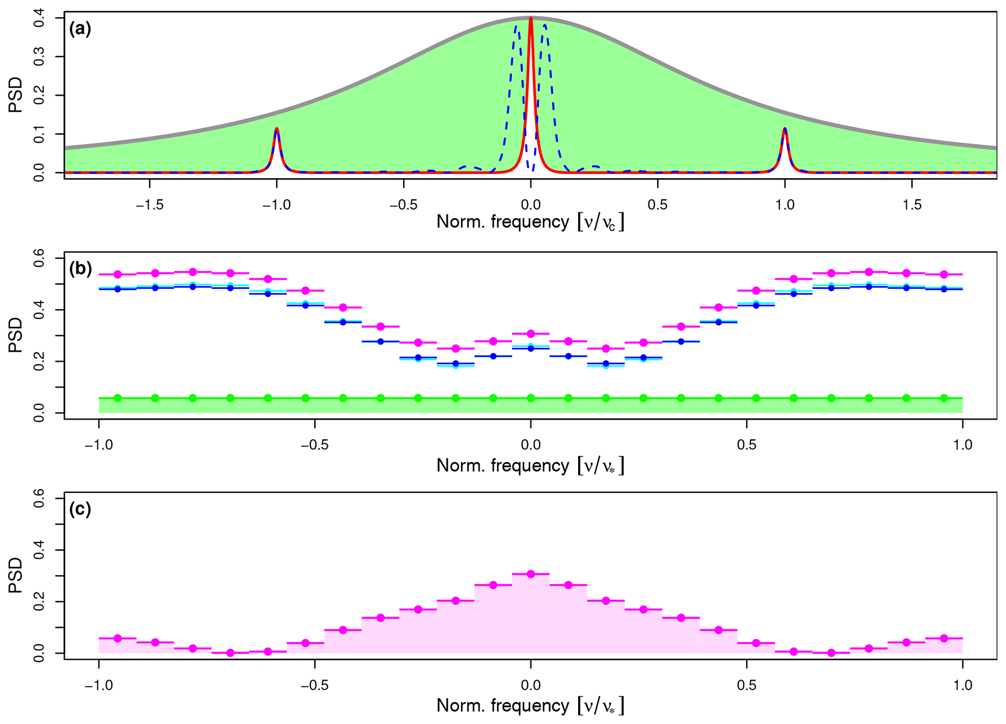
Figure 5Illustration of the method for estimating timescale-dependent reconstruction uncertainties in the spectral domain, shown for the uncertainty components 𝒰(1) and 𝒰(2) which are based on the stochastic component X(t) of the supposed true climate signal. (a) Power spectral density SX(ν) (gray line) of this signal component, defined on a continuous and infinite frequency axis (normalized by the seasonal cycle frequency ), together with the product (red line) and the product (blue line). The green area equals the integral , as it appears in Eq. (59), which measures the variance of the white noise error component caused by sampling only a finite number of signal carriers. (b) The same white noise variance (green area) but divided by N (the number of signal carriers) after spectral aliasing and leakage have been applied to obtain the power spectral density (green dots), defined by Eq. (61), on a finite and discrete frequency axis now normalized by the Nyquist frequency , together with (blue dots), defined by Eq. (60), and (magenta dots), defined by Eq. (62). Cyan dots indicate the same as blue dots but neglect the effect of spectral leakage for comparison. (c) The product (magenta dots), the integral of which (magenta area) equals the squared reconstruction uncertainty , defined by Eq. (111).
This power spectral density is shown in Fig. 5a by the gray line. According to the reconstruction uncertainty model defined in Sect. 2, SX(ν) is decomposed into two components: (i) |C(ν)|2SX(ν), shown by the red line, the integral of which equals the variance of Un defined by Eq. (44) and where |C(ν)|2 (shown in Fig. 2a) acts as a spectral transfer function on SX(ν); (ii) [1−|C(ν)|2]SX(ν), the integral of which, indicated by the green area, equals the variance of the white noise component defined by Eq. (45). If SX(ν) is multiplied by the squared modulus of the error transfer function (shown in Fig. 2b), the component , shown by the blue line, is obtained, the integral of which equals the variance of FX,n defined by Eq. (52).
This component (blue dots), as well as the white noise component (green dots), is shown again in Fig. 5b but after spectral aliasing and leakage have been applied according to the sampling and measurement procedure described in Sect. 2.3. These components represent the discretized power spectral densities and . Note that the broad peaks at nonzero frequencies in Fig. 5b are direct images of the low-frequency peaks in Fig. 5a (blue line), whereas the bump centered at ν=0 represents the summed aliases of the high-frequency peaks in Fig. 5a (blue line) at ±kνc. Without proxy seasonality (τp=1 year), those peaks do not exist, and, thus, the power spectrum in Fig. 5b falls off to near zero at ν=0. Only spectral leakage may then lead to nonzero at ν=0, although in the example shown here the effect of the leakage is small (cyan dots). However, in cases with small T (implying large Δν), spectral leakage can provide a relevant contribution of power at ν=0 as the power from the neighboring broad spectral peaks is then effectively redistributed to the center of the frequency domain. This contribution is particularly important if the uncertainty of the time average over the entire proxy record is computed by setting τ0=T in Eq. (111) as in this case it is the only contribution to .
Finally, the sum of the abovementioned components, given by , is shown by the magenta dots in Fig. 5c. By multiplying this summed power spectral density by the spectral transfer function of the discrete moving average window mentioned above and then integrating it, we obtain the squared reconstruction uncertainty after smoothing, , defined by Eq. (111) and shown by the magenta area in Fig. 5c.
Likewise, one can define other timescale-dependent uncertainty metrics. For example, one might be interested in the uncertainty of the difference between the time averages over two periods of length T1 and T2, which are separated in time by the interval , measured from center to center. This can be expressed by the variance
if it were to be computed for the uncertainty components based on X(t) and where T1, T2 and δt are multiples of Δt. Then, using the Wiener–Khintchine theorem, we obtain the difference uncertainty metric
where denotes the inverse discrete Fourier transform of a sequence xm. Note that in this form the abovementioned difference uncertainty metric is valid only for stationary uncertainty components. If the seasonal cycle amplitude is constant over time (i.e., no orbital variations), then all uncertainty components are stationary. If orbital variations are taken into account, however, only 𝒰(1) and 𝒰(2) are stationary, as shown in Sect. 3. For the components 𝒰(3),n, 𝒰(4),n, and ℬn, the difference metric, in this case, had to be computed directly from their time domain expressions; see Eqs. (87), (89), and (92), respectively.
To conclude this section, we briefly present an example of the time series and power spectra of the reconstruction bias ℬn and of the reconstruction uncertainty components 𝒰(3),n and 𝒰(4),n. Specifically, we set years, year, Δt=100 years, years, and N=5. Furthermore, the deterministic signal is specified in this example by the parameters , , , , , and , which implies that the amplitude of the seasonal cycle decreases during the 10 100 years, as is the case during the Holocene. According to the proxy seasonality parameter values chosen here, the bias ℬn is positive and exhibits a negative trend, as shown in Fig. 6a (cyan line). Likewise the uncertainty components 𝒰(3),n and 𝒰(4),n also decrease over time (blue and green lines). Since the orbital modulation frequency νa is located on the discrete frequency axis between ν0 and ν1, its power spectral density is distributed by spectral leakage across all frequencies. This yields a highly red power spectrum of ℬn and 𝒰(3),n, shown in Fig. 6b. Thus, at high frequencies the summed power spectral densities (dashed black line) and (dashed gray line) are dominated by the white noise component, whereas at low frequencies they are dominated by the effect of orbital variations. Hence, if we were to compute the timescale-dependent uncertainty metric (Eq. 111) but for 𝒰(3),n and 𝒰(4),n, denoted by , the uncertainty would shrink only slowly for increasing values of τ0 because the orbital variations are associated with a highly correlated error in time at long timescales.
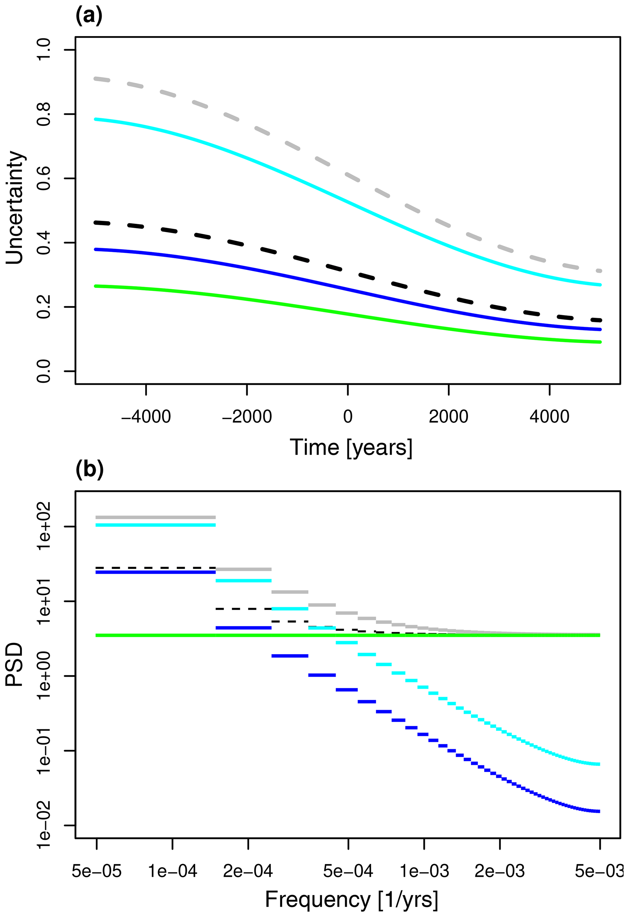
Figure 6Example of the reconstruction uncertainty based on the deterministic component Y(t) of the supposed true climate signal. (a) Time series of the reconstruction bias ℬn (cyan line), of the uncertainty components 𝒰(3),n (blue line) and 𝒰(4),n (green line), of (dashed black line), and (dashed gray line). (b) Power spectral densities of the corresponding error components: Sℬ,m (cyan line), (blue line), (green line), (dashed black line), and (gray line).
To allow for an analytic treatment of the problem, the method for estimating timescale-dependent reconstruction uncertainties, presented in Sects. 2 to 4, is necessarily based on a number of simplifying assumptions.
-
We assume a fixed proxy seasonality in the sense of applying every year the same seasonal timing of a prescribed proxy abundance period, characterized by the parameters τp and ϕc. For this reason we have to separate the supposed true climate signal into a stochastic component X(t) and a deterministic component Y(t) that represents the seasonal cycle because proxy seasonality then implies an in-phase subsampling from Y(t) which, in turn, affects the amount of variance aliased from the seasonal cycle 𝒰(4),n and which may also lead to a reconstruction bias ℬn and associated uncertainty 𝒰(3),n. This scenario represents the extreme case where a seasonal abundance period is completely imposed on the proxy by an external process (see, for example, Leduc et al., 2010), such as, for example, seasonally determined nutrient supply possibly controlled by the seasonality of solar irradiance or oceanic upwelling. By contrast, in the opposite extreme case where no seasonality is imposed at all, we do not need to separate the climate signal into X(t) and Y(t). In this case the total climate signal is fully recorded by the proxy, but its total variance is reduced by some factor because of habitat tracking if the habitat PDF of the proxy is narrower than the PDF of the climate signal. According to the idea of Mix (1987), this factor can be obtained by multiplying the two PDFs, and it may possibly also be expressed as a frequency-dependent spectral transfer function. This scenario corresponds to setting τp=1 year in our method and subsequently multiplying the obtained error power spectrum by the aforementioned transfer function. Hence, if we introduce some parameter, , that measures the extent to which seasonality is imposed for a specific proxy record (with s=0 indicating no imposition of seasonality), then we may express the actual uncertainty as a linear combination of the uncertainties obtained from the abovementioned two extreme scenarios, weighted by s and by 1−s, respectively. Note, however, that the effects of seasonality can be rather complex (see, for example, Jonkers and Kučera, 2017), depending on the type of proxy used, and, thus, the optimal strategy for modeling the associated uncertainties depends on the specific application.
-
We neglect calibration errors representing uncertainties regarding the climate–proxy relationship. Assuming this relationship is linear and is obtained by linear regression, errors of this type may have two effects. Uncertainties in the intercept parameter will introduce a reconstruction uncertainty that is constant in time like the bias uncertainty 𝒰(3),n (in the case without orbital variations). Uncertainties in the slope parameter, on the other hand, will introduce a frequency-independent uncertainty in the error variance. The mean of the possible error variances, however, might be close to the variance obtained from our method unless the PDF of the obtained error variances is strongly skewed. If the climate–proxy relationship is non-linear, or if there are uncertainties regarding the linearity itself, modeling of the implied uncertainties might be more complex, although it should still be possible to decompose those errors into a bias and a variance component.
-
We assume a constant sediment accumulation rate and a constant bioturbation depth, and we also assume regular sampling from the sediment core and neglect dating uncertainties, although relaxing these assumptions may generate additional uncertainties of noticeable magnitude. For example, the relevance of dating uncertainties is demonstrated by Goswami et al. (2014) and Boers et al. (2017). If these sources of uncertainty are treated in a stochastic sense, they could, in principle, be included in our approach by allowing for correlated sampling jitter ϵ, the mathematical basis of which is given by Balakrishnan (1962) (see also Moore and Thomson, 1991). More generally, these uncertainties could be modeled by allowing for a variable time–depth relationship and perhaps by also allowing for the nonstationarity of the uncertainty components 𝒰1 and 𝒰2 to represent variations of the smoothing timescales τb and τs.
From the above, it turns out that, in its current form, the method is neither complete in terms of processes affecting the reconstruction uncertainty nor does it cover all possible reconstruction scenarios in terms of proxy type and application context. However, our formulation of the method outlines a conceptually and mathematically well-founded approach of how timescale-dependent reconstruction uncertainties could, and probably should, be estimated – in particular, when systematic and exact quantification is required. This latter point is highly relevant, for example, in the context of comparisons between circulation models and paleo-observations (e.g., Lohmann et al., 2013; Laepple and Huybers, 2014; Matsikaris et al., 2016) or likewise for any reanalysis efforts (e.g., Hakim et al., 2016) if data obtained from proxy records are involved. Thus, the fact that some of the neglected sources of uncertainty might be large compared to what is gained by our exact mathematical treatment does not qualify our approach as overly precise. The approach rather demonstrates the directions for future efforts in quantitative uncertainty estimation. As discussed above, our current formulation of the method may indeed be extended beyond the simplifications made. But as mathematical complexity increases in such case, extended formulations should be tailored to specific applications. In this sense, our formulation provides a minimal basis for the development of future uncertainty estimation methods.
Furthermore, the timescale-dependent uncertainties obtained from our method depend explicitly on assumptions regarding the structure of the supposed true climate signal X(t)+Y(t), although this climate signal is the unknown quantity to be reconstructed from the proxy record. However, it is an inevitable fact that the timescale-dependent reconstruction uncertainties do actually depend on this structure, a fact that is made obvious by our method and likewise by Amrhein (2020). One possible approach towards solving this problem would be an iterative procedure: (i) assume a specific structure for the supposed true climate signal; (ii) apply our method to obtain reconstruction uncertainties for a given proxy record; (iii) check whether the reconstructed signal is consistent under the obtained uncertainties with the assumed structure given its spectral or auto-correlation properties; and (iv) if this is not the case, update the assumptions and repeat these steps.
Finally, although our method provides an advancement in the quantification of reconstruction uncertainties, it also introduces a number of model parameters which are associated with their own uncertainty. However, if we are to improve quantitative uncertainty estimates, our reconstruction uncertainty model helps to identify those parameters which are most important and, therefore, need to be determined at higher precision. For example, how much seasonality is imposed on a certain proxy at a given geographical location within a specific local ecological system? On the other hand, it is possible to investigate how parameter uncertainties translate into reconstruction uncertainties, as was shown for the seasonal phase parameter ϕc. Nonetheless, the eventual benefit of uncertainty estimation methods like the one presented in this study and of extensions based thereon has still to be worked out in the future by systematically applying such methods to real data.
The present study introduces a method, the so-called Proxy Spectral Error Model (PSEM; see also Part 2 of this study by Dolman et al., 2020), for estimating timescale-dependent uncertainties of paleoclimate reconstructions obtained from single sediment proxy records. The method is based on an uncertainty model that takes into account proxy seasonality (together with orbital variations of the seasonal cycle amplitude), bioturbation, archive sampling parameters, and the effects of measuring only a finite number of signal carriers. For this model, analytic expressions are derived for the power spectrum of the reconstruction error from which timescale-dependent reconstruction uncertainties can be obtained. This approach is motivated by the fact that the spectral structure of the error is equivalent to its auto-correlation structure which, in turn, determines how archive smoothing, sampling, and averaging timescales affect the uncertainties. Various timescale-dependent uncertainty metrics can be defined and then computed from the error power spectrum by multiplying the spectrum by specific transfer functions and then integrating. This corresponds, in the time domain, to additional postprocessing steps performed on the reconstructed time series. For example, it is possible to investigate the uncertainty reduction achieved by a low pass filter with a given cut-off timescale or to quantify the uncertainty of the difference between two time averages with given averaging timescales.
The method proves useful in different ways. First, it can serve to obtain quantitative uncertainty estimates for practical applications in paleoclimate science. This is demonstrated in Part 2 of this study (Dolman et al., 2020) in which a number of application examples are presented. Second, the derived analytic expressions can be used to acquire a better qualitative understanding of the structure of the uncertainties. In particular, we can conclude the following.
-
The reconstruction uncertainties can be decomposed into two components. The first is a component whose variance is obtained by multiplying the power spectrum of the supposed true climate signal by a transfer function and then integrating. This so-called error transfer function has a structure corresponding to a bandpass filter with its cut-off timescales given by the longest applied archive smoothing timescale and by a suitably chosen reference smoothing timescale (by analogy with the transfer function discussed by Amrhein, 2020). Thus, multiplying the spectrum by the error transfer function corresponds to applying that bandpass filter to the supposed true climate signal. The second is a white noise component that scales inversely with the number of signal carriers retrieved from each slice of sediment (and being subject to the same single laboratory measurement). Thus, in the asymptotic limit of infinitely many signal carriers, this component vanishes. In the opposite limit, with only a single signal carrier being measured from each slice, the variance of this component equals the variance that is contained in the supposed true climate signal at timescales shorter than the longest applied archive smoothing timescale. This component corresponds to what is referred to, according to Dolman and Laepple (2018), as the noise created by the aliasing of variability from interannual and intra-annual timescales. Depending on geographical location and climatic conditions, this white noise uncertainty component may be dominated by ENSO variability or by the seasonal cycle, for example.
-
In the presence of proxy seasonality such that the climate signal is recorded by the proxy only during a limited seasonal window each year, the abovementioned error transfer function has additional high-frequency peaks at the seasonal cycle frequency and at its higher harmonics, and, thus, it corresponds to a multi-bandpass filter in this case. In consequence of this, a certain amount of variance is reallocated from the abovementioned white noise uncertainty component to the first component, although it appears there at the lowest frequencies because of spectral aliasing. Thus, proxy seasonality may generate uncertainties that are highly correlated in the time domain. In most cases, this low-frequency uncertainty will be dominated by the seasonal cycle and its amplitude modulation caused by orbital variations (as demonstrated by Huybers and Wunsch, 2003, for example). Nonetheless, if the stochastic climate variability is only weakly red such that it is associated with notable power near the seasonal cycle frequency, it may also give rise to low-frequency uncertainties, in particular if the seasonal cycle is weak by comparison.
-
If, in addition, the proxy abundance window is known to have a preferred seasonal timing throughout the year, then the contribution that the seasonal cycle signal (with its deterministic phase) makes to both of the abovementioned two uncertainty components is further modified. The white noise component can be larger or smaller than for random seasonal timing, and, in particular, the first uncertainty component may include a (potentially time-varying) deterministic bias in this case. Moreover, the sum of their variances may change because of the in-phase subsampling from a deterministic signal.
-
Uncertainties caused by laboratory measurement errors are independent of the abovementioned components, and, thus, the associated power spectral density can simply be added to the error power spectrum obtained from our method. In practice, this uncertainty component is assumed to be white noise such that it scales inversely with any averaging timescale.
Another interesting and future application of the derived analytic expressions would be the inference of the power spectrum of the true climate signal. Specifically, by setting the reference climate in our method to zero and then repeating the entire derivation, one obtains the analytic expressions for the power spectrum of the climate reconstruction itself rather than of its error. Thus, one obtains an operator that transforms the power spectrum of the supposed true climate signal into a spectrum subject to the distortions caused by the processes included in our reconstruction uncertainty model. Then, given all of the parameters of the uncertainty model, and assuming a parametric form for the true climate signal, it might be possible to estimate its parameters by means of a maximum likelihood approach (that investigates the likelihood, under a given set of parameters, of the power spectrum estimated from a specific proxy record). This essentially amounts to inverting the aforementioned operator, which is similar to the correction technique used by Laepple and Huybers (2013) and motivated by the anti-aliasing approach of Kirchner (2005).
The variance of is given by its auto-covariance function at lag zero, . By substitution from Eq. (73), it can be shown, after some algebraic transformations, that
with
where
and the characteristic function differences D1 to D8, also using definition (33), are given by
Since the auto-covariance contributions R3, R4, R7, and R8 depend on tn, the variance of is nonstationary. Furthermore, it turns out that with the characteristic function differences D1 to D8 are all zero, and, thus, the auto-covariance contributions R1 to R8 are all zero. This implies that the auto-covariance function of is nonzero only at lag zero () and zero at all other lags (). Hence, is a white noise process, and from its definition (Eq. 73) it follows that it has zero mean. Note that Eq. (A4) is identical to Eq. (49) in Sect. 3.1 but with ν=νc, and so the abovementioned procedure follows the same key idea (according to the approach of Balakrishnan, 1962) of extrapolating the auto-covariance function from nonzero lags towards lag zero.
From the abovementioned expressions, we can write the variance of as
with the amplitude of the stationary variance component,
the amplitude of the variance component oscillating at frequency νa,
and the amplitudes of the variance components oscillating at frequency 2νa,
and where
and
and ϕb1 and Mb1 are defined by Eqs. (77) and (78), respectively. The time average of this variance over an infinitely long time interval is then given by , provided that Δt is not a multiple of . If the time average is taken over a finite time interval of length T, centered at t=0, the time mean variance is given by
provided that .
| Parameter | Symbol |
| Seasonal cycle variance | |
| Seasonal cycle frequency | νc |
| Expected seasonal cycle phase | |
| Seasonal phase uncertainty | |
| Amplitude modulation variance | |
| Amplitude modulation frequency | νa |
| Amplitude modulation phase | ϕa |
| Proxy abundance timescale | τp |
| Bioturbation timescale | τb |
| Sediment sampling timescale | τs |
| Sampling interval | Δt |
| Length of proxy record | T |
| Number of signal carriers | N |
| Measurement error variance | |
| Reference climate averaging timescale | τr |
No data sets were used in this article.
TL developed the underlying idea of the Proxy Spectral Error Model. TK, AMD, and TL designed the conceptual outline of the research. TK laid out and performed the mathematical derivation of the analytic expressions and wrote the paper based on numerous discussions with AMD and TL.
The authors declare that they have no conflict of interest.
This article is part of the special issue “Paleoclimate data synthesis and analysis of associated uncertainty (BG/CP/ESSD inter-journal SI)”. It is not associated with a conference.
This is a contribution to the European Research Council (ERC) project SPACE. The work profited from discussions at the Climate Variability Across Scales (CVAS) working group of the Past Global Changes (PAGES) program. We thank Cristian Proistosescu (University of Illinois Urbana-Champaign) for bringing to our awareness the formalism to describe the effects of jittered sampling in signal processing and Dan Amrhein (University of Washington) for discussions on the spectral uncertainty approach. We also thank Shinya Nakano and one anonymous referee for their useful comments which helped to improve this work.
This research has been supported by the European Research Council (ERC) project SPACE, which has received funding from the ERC under the European Union’s Horizon 2020 research and innovation program (grant agreement no. 716092). Andrew M. Dolman was supported by the German Federal Ministry of Education and Research (BMBF) through the PALMOD project (FKZ: 01LP1509C).
This paper was edited by Denis-Didier Rousseau and reviewed by Shinya Nakano and one anonymous referee.
Amrhein, D. E.: How large are temporal representativeness errors in paleoclimatology?, Clim. Past, 16, 325–340, https://doi.org/10.5194/cp-16-325-2020, 2020. a, b, c, d, e, f
Balakrishnan, A. V.: On the problem of time jitter in sampling., IRE Trans. Inf. Theory, IT-8, 226–236, 1962. a, b, c, d, e
Berger, W. H. and Heath, G. R.: Vertical mixing in pelagic sediments, J. Mar. Res., 26, 134–143, 1968. a, b
Birks, H. J. B. and Seppä, H.: Pollen-based reconstructions of late-Quaternary climate in Europe – progress, problems, and pitfalls, Acta Palaeobot., 44, 317–334, 2004. a
Boers, N., Goswami, B., and Ghil, M.: A complete representation of uncertainties in layer-counted paleoclimatic archives, Clim. Past, 13, 1169–1180, https://doi.org/10.5194/cp-13-1169-2017, 2017. a
Dee, S., Emile-Geay, J., Evans, M. N., Steig, E. J., and Thompson, D. M.: PRYSM: an open-source framework for PRoxY System Modeling, with applications to oxygen-isotope systems, J. Adv. Model. Earth Sy., 7, 1220–1247, 2015. a
Dolman, A. M. and Laepple, T.: Sedproxy: a forward model for sediment-archived climate proxies, Clim. Past, 14, 1851–1868, https://doi.org/10.5194/cp-14-1851-2018, 2018. a, b, c
Dolman, A. M., Kunz, T., Groeneveld, J., and Laepple, T.: Estimating the timescale-dependent uncertainty of paleoclimate records – a spectral approach. Part II: Application and interpretation, Clim. Past Discuss., https://doi.org/10.5194/cp-2019-153, in review, 2020. a, b, c, d, e
Evans, M. N., Tolwinski-Ward, S. E., Thompson, D. M., and Anchukaitis, K. J.: Applications of proxy system modeling in high resolution paleoclimatology, Quaternary Sci. Rev., 76, 16–28, 2013. a
Goreau, T. J.: Frequency sensitivity of the deep-sea climatic record, Nature, 287, 620–622, 1980. a
Goswami, B., Heitzig, J., Rehfeld, K., Marwan, N., Anoop, A., Prasad, S., and Kurths, J.: Estimation of sedimentary proxy records together with associated uncertainty, Nonlin. Processes Geophys., 21, 1093–1111, https://doi.org/10.5194/npg-21-1093-2014, 2014. a
Greaves, M., Caillon, N., Rebaubier, H., Bartoli, G., Bohaty, S., Cacho, I., Clarke, L., Cooper, M., Daunt, C., Delaney, M., deMenocal, P., Dutton, A., Eggins, S., Elderfield, H., Garbe-Schoenberg, D., Green, E. G. D., Groeneveld, J., Hastings, D., Hathorne, E., Kimoto, K., Klinkhammer, G., Labeyrie, L., Lea, D. W., Marchitto, T., Martínez-Botí, M. A., Mortyn, P. G., Ni, Y., Nuernberg, D., Paradis, G., Pena, L., Quinn, T., Rosenthal, Y., Russell, A., Sagawa, T., Sosdian, S., Stott, L., Tachikawa, K., Tappa, E., Thunell, R., and Wilson, P. A.: Interlaboratory comparison study of calibration standards for foraminiferal Mg/Ca thermometry, Geochem. Geophy. Geosy., 9, 1–27, 2008. a
Hakim, G. J., Emile-Geay, J., Steig, E. J., Noone, D., Anderson, D. M., Tardif, R., Steiger, N., and Perkins, W. A.: The last millennium climate reanalysis project: framework and first results, J. Geophys. Res.-Atmos., 121, 6745–6764, 2016. a
Huybers, P. and Wunsch, C.: Rectification and precession signals in the climate system, Geophys. Res. Lett., 30, 2011, https://doi.org/10.1029/2003GL017875, 2003. a, b
Johnsen, S. J.: Stable isotope homogenization of polar firn and ice, in: Isotopes and impurities in snow and ice, no. 118, proceedings of the Grenoble symposium 1975, IAHS-AISH Publication, Grenoble, France, 210–219, 1977. a
Jonkers, L. and Kučera, M.: Global analysis of seasonality in the shell flux of extant planktonic Foraminifera, Biogeosciences, 12, 2207–2226, https://doi.org/10.5194/bg-12-2207-2015, 2015. a
Jonkers, L. and Kučera, M.: Quantifying the effect of seasonal and vertical habitat tracking on planktonic foraminifera proxies, Clim. Past, 13, 573–586, https://doi.org/10.5194/cp-13-573-2017, 2017. a
Jouzel, J., Alley, R. B., Cuffey, K. M., Dansgaard, W., Grootes, P., Hoffmann, G., Johnsen, S. J., Koster, R. D., Peel, D., Shuman, C. A., Stievenard, M., Stuiver, M., and White, J.: Validity of the temperature reconstruction from water isotopes, J. Geophys. Res.-Oceans, 102, 26471–26487, 1997. a
Kirchner, J. W.: Aliasing in 1∕fα noise spectra: origins, consequences, and remedies, Phys. Rev. E, 71, https://doi.org/10.1103/physreve.71.066110, 2005. a
Laepple, T. and Huybers, P.: Reconciling discrepancies between Uk37 and Mg/Ca reconstructions of Holocene marine temperature variability, Earth Planet. Sc. Lett., 375, 418–429, 2013. a
Laepple, T. and Huybers, P.: Ocean surface temperature variability: large model–data differences at decadal and longer periods, P. Natl. Acad. Sci. USA, 111, 16682–16687, 2014. a
Laepple, T., Münch, T., Casado, M., Hoerhold, M., Landais, A., and Kipfstuhl, S.: On the similarity and apparent cycles of isotopic variations in East Antarctic snow pits, The Cryosphere, 12, 169–187, https://doi.org/10.5194/tc-12-169-2018, 2018. a
Laepple, T., Werner, M., and Lohmann, G.: Synchronicity of Antarctic temperatures and local solar insolation on orbital timescales, Nature, 471, 91–94, 2011. a
Leduc, G., Schneider, R., Kim, J.-H., and Lohmann, G.: Holocene and Eemian sea surface temperature trends as revealed by alkenone and Mg/Ca paleothermometry, Quaternary Sci. Rev., 29, 989–1004, 2010. a
Lohmann, G., Pfeiffer, M., Laepple, T., Leduc, G., and Kim, J.-H.: A model–data comparison of the Holocene global sea surface temperature evolution, Clim. Past, 9, 1807–1839, https://doi.org/10.5194/cp-9-1807-2013, 2013. a, b
Matsikaris, A., Widmann, M., and Jungclaus, J.: Influence of proxy data uncertainty on data assimilation for the past climate, Clim. Past, 12, 1555–1563, https://doi.org/10.5194/cp-12-1555-2016, 2016. a
Mix, A.: The Oxygen-Isotope Record of Glaciation, in: North America and Adjacent Oceans during the Last Deglaciation, vol. K-3 of Geology of North America, Geol. Soc. Am., 3, 111–135, 1987. a
Moore, M. I. and Thomson, P. J.: Impact of jittered sampling on conventional spectral estimates., J. Geophys. Res., 96, 18519–18526, 1991. a, b, c
Münch, T. and Laepple, T.: What climate signal is contained in decadal- to centennial-scale isotope variations from Antarctic ice cores?, Clim. Past, 14, 2053–2070, https://doi.org/10.5194/cp-14-2053-2018, 2018. a
Nürnberg, D., Bijma, J., and Hemleben, C.: Assessing the reliability of magnesium in foraminiferal calcite as a proxy for water mass temperatures, Geochim. Cosmochim. Ac., 60, 803–814, 1996. a
Priestley, M. B.: Spectral analysis and time series, Academic Press, London, UK, New York, USA, 1981. a, b, c, d, e, f, g
Reschke, M., Rehfeld, K., and Laepple, T.: Empirical estimate of the signal content of Holocene temperature proxy records, Clim. Past, 15, 521–537, https://doi.org/10.5194/cp-15-521-2019, 2019. a, b
Rosell-Melé, A., Bard, E., Emeis, K.-C., Grimalt, J. O., Müller, P., Schneider, R., Bouloubassi, I., Epstein, B., Fahl, K., Fluegge, A., Freeman, K., Goñi, M., Güntner, U., Hartz, D., Hellebust, S., Herbert, T., Ikehara, M., Ishiwatari, R., Kawamura, K., Kenig, F., de Leeuw, J., Lehman, S., Mejanelle, L., Ohkouchi, N., Pancost, R. D., Pelejero, C., Prahl, F., Quinn, J., Rontani, J.-F., Rostek, F., Rullkotter, J., Sachs, J., Blanz, T., Sawada, K., Schulz-Bull, D., Sikes, E., Sonzogni, C., Ternois, Y., Versteegh, G., Volkman, J., and Wakeham, S.: Precision of the current methods to measure the alkenone proxy and absolute alkenone abundance in sediments: results of an interlaboratory comparison study, Geochem. Geophy. Geosy., 2, 2000GC0, https://doi.org/10.1029/2000GC000141, 2001. a
Thirumalai, K., Partin, J. W., Jackson, C. S., and Quinn, T. M.: Statistical constraints on El Niño Southern Oscillation reconstructions using individual foraminifera: a sensitivity analysis, Paleoceanography, 28, 401–412, 2013. a
Tierney, J. E. and Tingley, M. P.: A Bayesian, spatially-varying calibration model for theTEX86 proxy, Geochim. Cosmochim. Ac., 127, 83–106, 2014. a
Whillans, I. M. and Grootes, P. M.: Isotopic diffusion in cold snow and firn, J. Geophys. Res., 90, 3910–3918, 1985. a
- Abstract
- Introduction
- Reconstruction uncertainty model
- Spectral representation of reconstruction uncertainty
- Timescale-dependent reconstruction uncertainty
- Discussion
- Conclusions
- Appendix A: Nonstationary variance of the white noise component
- Appendix B: Parameters of the reconstruction uncertainty model as defined in Sect. 2
- Data availability
- Author contributions
- Competing interests
- Special issue statement
- Acknowledgements
- Financial support
- Review statement
- References