the Creative Commons Attribution 4.0 License.
the Creative Commons Attribution 4.0 License.
 | 09 Jul 2020
Mysteriously high Δ14C of the glacial atmosphere: influence of 14C production and carbon cycle changes
Ashley Dinauer
Florian Adolphi
Fortunat Joos
Despite intense focus on the ∼190 ‰ drop in atmospheric Δ14C during Heinrich Stadial 1 at ∼17.4–14.6 ka, the specific mechanisms responsible for the apparent Δ14C excess in the glacial atmosphere have received considerably less attention. The computationally efficient Bern3D Earth system model of intermediate complexity, designed for long-term climate simulations, allows us to address a very fundamental but still elusive question concerning the atmospheric Δ14C record: how can we explain the persistence of relatively high Δ14C values during the millennia after the Laschamp event? Large uncertainties in the pre-Holocene 14C production rate, as well as in the older portion of the Δ14C record, complicate our qualitative and quantitative interpretation of the glacial Δ14C elevation. Here we begin with sensitivity experiments that investigate the controls on atmospheric Δ14C in idealized settings. We show that the interaction with the ocean sediments may be much more important to the simulation of Δ14C than had been previously thought. In order to provide a bounded estimate of glacial Δ14C change, the Bern3D model was integrated with five available estimates of the 14C production rate as well as reconstructed and hypothetical paleoclimate forcing. Model results demonstrate that none of the available reconstructions of past changes in 14C production can reproduce the elevated Δ14C levels during the last glacial. In order to increase atmospheric Δ14C to glacial levels, a drastic reduction of air–sea exchange efficiency in the polar regions must be assumed, though discrepancies remain for the portion of the record younger than ∼33 ka. We end with an illustration of how the 14C production rate would have had to evolve to be consistent with the Δ14C record by combining an atmospheric radiocarbon budget with the Bern3D model. The overall conclusion is that the remaining discrepancies with respect to glacial Δ14C may be linked to an underestimation of 14C production and/or a biased-high reconstruction of Δ14C over the time period of interest. Alternatively, we appear to still be missing an important carbon cycle process for atmospheric Δ14C.
- Article
(8898 KB) - Full-text XML
-
Supplement
(2046 KB) - BibTeX
- EndNote


The cosmogenic radionuclide radiocarbon (14C) is a powerful tracer for the study of several ocean processes including deep ocean circulation and ventilation. Past changes in atmospheric 14C∕C (i.e., Δ14Catm, in per mill; corresponding to Δ from Stuiver and Polach, 1977), as recorded in absolutely dated tree rings, plant macrofossils, speleothems, corals, and foraminifera, have been interpreted as possibly reflecting real changes in the ocean's large-scale overturning circulation (Siegenthaler et al., 1980). The extended 54 000-year record of Δ14Catm from the latest IntCal compilation (i.e., IntCal13; Reimer et al., 2013) and from two Hulu Cave stalagmites (Cheng et al., 2018), adjusted to the presently accepted value of the radiocarbon half-life of 5700 years (Audi et al., 2003; Bé et al., 2013), suggests that large millennial-scale variations in Δ14Catm occurred during the last glacial compared to the relatively small (∼30 ppm) change in atmospheric CO2 over the same time period (Fig. 1). When interpreting the implications of such changes, it is important to note that Δ14Catm is controlled not only by global carbon cycle processes but also by variations in the atmospheric 14C production rate. Therefore, the use of Δ14Catm as an indicator of past oceanic conditions, particularly those associated with air–sea exchange efficiency and deep ocean ventilation rates, requires reliable estimates of the 14C production rate over time.

Figure 1Comparison of various paleoclimate records for the last 54 kyr. (a) Atmospheric CO2 from the data compilation of Köhler et al. (2017). The light red envelope shows the uncertainty (2σ). (b) Atmospheric Δ14C reconstructed from 14C measurements on tree rings, plant macrofossils, speleothems, corals, and foraminifera. The light blue envelope shows the uncertainty (2σ) in the IntCal13 calibration curve (Reimer et al., 2013), whereas the Hulu Cave data (Cheng et al., 2018) are shown with error bars (1σ). Hulu Cave data are consistent with IntCal13 between ∼10.6 and 33.3 ka. For both records Δ14C values were adjusted to the presently accepted value of the radiocarbon half-life (5700 years). (c) 14C production rate in relative units reconstructed from paleointensity data (Laj et al., 2000, 2004; Nowaczyk et al., 2013; Channell et al., 2018) and from polar ice-core 10Be fluxes (Adolphi et al., 2018). The heavy dark gray line is the mean paleointensity-based 14C production rate. (d) Global benthic δ18O stack, a proxy for ice volume, from Lisiecki and Stern (2016). Three vertical light gray bars indicate the Laschamp excursion (∼41 ka) when the Earth's geomagnetic dipole field intensity was close to zero, the Mono Lake geomagnetic excursion (∼34 ka), and the last glacial termination (∼18 to 11 ka).
The vast majority of all 14C production changes are the result of either solar or geomagnetic modulation of the cosmic ray flux reaching the Earth (Masarik and Beer, 1999; Poluianov et al., 2016). Figure 1 shows several different proxy records of the global production rate of 14C in relative units covering the full range of the 14C dating method based on geomagnetic field data from marine sediments (Laj et al., 2000, 2004; Nowaczyk et al., 2013; Channell et al., 2018) and on 10Be and 36Cl measurements in polar ice cores (Adolphi et al., 2018). A fundamental difference between these reconstruction methods is that paleointensity-based estimates of the 14C production rate, by definition, do not reflect changes in the solar modulation of the cosmic radiation, whereas ice-core 10Be-based estimates give the combined influence of solar and geomagnetic modulation on radionuclide production. Of note is the striking coherence in all three records (Δ14Catm, paleointensity-based production, and ice-core 10Be-based production) of the Laschamp excursion (∼41 ka), when the Earth's geomagnetic dipole field briefly reversed and its intensity was close to zero (Nowaczyk et al., 2012; Laj et al., 2014). According to reconstructions and production rate models, this large geomagnetic event caused a doubling of the 14C production rate, leading to the highest Δ14Catm values over the last 54 kyr. Relatively high Δ14Catm values continued until ∼25 ka, then gradually diminished to preindustrial levels, interrupted by a sharp drop in Δ14Catm during Heinrich Stadial 1 (HS1) at ∼17.4 to 14.6 ka (sometimes called the “mystery interval”; Broecker and Barker, 2007). While the Laschamp geomagnetic excursion appears to be responsible for the Δ14Catm peak at ∼41 ka, the production rate estimates during much of the pre-Holocene period are subject to considerable uncertainty.
Paleointensity-based reconstructions are sensitive to coring disturbances of poorly consolidated sediments. The last 50 kyr are represented by the relatively slushy uppermost few meters of recovered marine sediment cores (Channell et al., 2018). Channell et al. (2018) preferentially selected cores recovered using conventional piston and square barrel gravity coring methods and from sites with high mean (>15 cm kyr−1) sedimentation rates to minimize the influence of drilling disturbance and reached very different production rates than, e.g., Laj et al. (2000). On the other hand, ice-core 10Be records are affected by changes in the transport and deposition of atmospheric 10Be, which may overprint the production rate changes (e.g., Heikkilä et al., 2013). Furthermore, in order to calculate the ice-core 10Be deposition fluxes, snow accumulation rates must be known for each specific ice core, which themselves have uncertainties on the order of 10 % to 20 % that propagate into the ice-core 10Be fluxes (Gkinis et al., 2014; Rasmussen et al., 2013). The large uncertainties associated with the reconstruction of past changes in 14C production hamper our ability to reliably predict the extent to which production changes contributed to high glacial Δ14Catm levels. Only if estimates of past changes in 14C production are robust can one improve assessments of the relative importance of the two fundamental mechanisms responsible for glacial–interglacial Δ14C changes: (1) production changes and (2) carbon cycle changes.
Earlier model studies have focused heavily on the ∼190 ‰ drop in Δ14Catm during HSI and on the deglacial trends in Δ14Catm after HS1 (Muscheler et al., 2004; Broecker and Barker, 2007; Skinner et al., 2010; Mariotti et al., 2016; Delaygue et al., 2003; Marchal et al., 2001; Huiskamp and Meissner, 2012; Hain et al., 2014). Historically, the younger portion of the Δ14Catm record has received more attention than the glacial section because of the early emphasis on the general climatic trends of the North Atlantic stadials (HS1 and the Younger Dryas, YD) and the Bølling–Allerød (BA) warm period, as well as on the important role of an exceptionally aged (14C-depleted) deepwater mass in the pulsed rise of atmospheric CO2 during the last glacial termination (e.g., Skinner et al., 2017). Less research over the last few decades has studied the specific mechanisms responsible for high glacial Δ14Catm levels. The model studies that are available point out the difficulties in simulating the correct glacial Δ14Catm levels (Hughen et al., 2004; Köhler et al., 2006). These studies demonstrate with box models that glacial levels of Δ14Catm cannot be attained without invoking significant changes in ocean circulation, air–sea gas exchange, and carbonate sedimentation. However, the box models were not able to reproduce Δ14Catm values higher than 700 ‰, and these results still need to be scrutinized with models of higher complexity. To our knowledge, no three-dimensional ocean biogeochemical model has yet simulated the 50 000-year record of Δ14Catm. Many questions remain unanswered, in particular the following: what mechanism can account for the persistence of relatively high Δ14Catm values during the millennia after the Laschamp excursion?
The expected timescale for sustaining elevated levels of Δ14Catm after a production peak is on the order of thousands of years, a timescale tied to the mean lifetime of 14C (∼8223 years; Audi et al., 2003; Bé et al., 2013) and the time required for deep ocean ventilation (on the order of 1000 years or more; Primeau, 2005). Specifically, Muscheler et al. (2004) demonstrate that the characteristic time constant for equilibration of Δ14Catm after a perturbation in atmospheric production is 5000 years. By this analysis, the Laschamp event, which lasted only about 1500 to 2000 years (Laj et al., 2000), was insufficient to sustain the high Δ14Catm values observed over the next ∼15 000 years. The lack of significant changes (only ∼10 %) in atmospheric CO2 during the time period of interest raises the question of what causes variations in Δ14Catm, but not CO2, on millennial timescales. The obvious answers are cosmic ray modulation and air–sea gas exchange. Ultimately, no explanation for high glacial Δ14Catm levels can be complete in the absence of more robust estimates of the pre-Holocene 14C production rate, as well as a good understanding of the ocean carbon cycle under glacial climate conditions.
One of the major challenges associated with modeling glacial–interglacial climate cycles is that it is currently not possible to reproduce climate and atmospheric CO2 variations on the basis of orbital forcing alone. Problems include the complexity of the Earth system, making it difficult to represent all the relevant processes in models, and the long timescales involved, making simulations covering tens of thousands of years costly in computation time. Glacial–interglacial simulations with dynamic ocean and land models of intermediate complexity have begun to emerge, but these models are not yet able to reproduce the reconstructed variations in important proxy data or the timing of CO2 variations during the last glacial termination (Brovkin et al., 2012; Ganopolski and Brovkin, 2017; Menviel et al., 2012). A wide variety of mechanisms, both physical and biological, centered on or connected with the ocean, as well as exchange processes with the land biosphere, marine sediments, coral reefs, and the lithosphere, are thought to play a role in explaining the glacial–interglacial variations in atmospheric CO2 (Archer et al., 2000; Fischer et al., 2010; Wallmann et al., 2016; Galbraith and Skinner, 2020), but how they interacted over time under the influence of orbital forcing remains elusive. We appear to still be missing a single framework in which these mechanisms are linked to each other in a predictable manner. As long as there are still large gaps in our understanding of the glacial climate and associated ocean carbon cycle, a convenient way to examine the impact of the possible mechanisms on atmospheric CO2 levels, and here on Δ14Catm, is to perform sensitivity experiments and scenario-based simulations with models. This allows us to investigate specific phenomena in idealized settings, permitting us to investigate in detail which parameters and processes are most important in controlling Δ14Catm levels.
In this paper we extend previous modeling efforts concerning the record of Δ14Catm with respect to three issues: (1) the sensitivity of the Δ14Catm response to carbon cycle changes and the potential importance of marine sediments, (2) the simulation of Δ14Catm covering the time range of the IntCal13 radiocarbon calibration curve (50 000 years), the primary focus being the explanation for high glacial Δ14Catm levels, and (3) a new 50 000-year record of the 14C production rate, as inferred by deconvolving the reconstructed histories of Δ14Catm and CO2 with a prognostic carbon cycle model and considering the uncertainties associated with the glacial–interglacial ocean carbon cycle. In the following sections we first introduce the Bern3D Earth system model of intermediate complexity and describe the carbon cycle scenarios for forcing it. We then use step changes in the 14C production rate and in selected parameters of the ocean carbon cycle model to gain insight into the transient and equilibrium response of Δ14Catm. After these sensitivity experiments we present the results of paleoclimate simulations forced by available reconstructions of past changes in 14C production together with reconstructed and hypothetical carbon cycle changes accompanying glacial–interglacial climate cycles. Finally, we present results for a first attempt to reconstruct the glacial history of the 14C production rate using the Bern3D model forced with reconstructed variations in Δ14Catm and CO2 as well as a wide range of carbon cycle scenarios. We end with a comparison of three fundamentally different (model-based, paleointensity-based, and ice-core 10Be-based) reconstructions of atmospheric 14C production.
2.1 Brief description of the Bern3D model
Simulations are performed with the computationally efficient Bern3D Earth system model of intermediate complexity (version 2.0), which is designed for long-term climate simulations over several tens of thousands of years. The Bern3D couples a frictional geostrophic 3-D ocean general circulation model (Edwards et al., 1998; Edwards and Marsh, 2005; Müller et al., 2006), a 2-D energy–moisture balance atmosphere model (Ritz et al., 2011), an ocean carbon cycle model (Müller et al., 2008; Tschumi et al., 2008; Parekh et al., 2008), a chemically active 10-layer ocean sediment model (Heinze et al., 1999; Tschumi et al., 2011; Roth et al., 2014; Jeltsch-Thömmes et al., 2019), and a four-box model representing carbon stocks in the terrestrial biosphere (Siegenthaler and Oeschger, 1987). The coarse-resolution ocean model is implemented on a 41×40 horizontal grid, with 32 logarithmically spaced layers in the vertical. The seasonal cycle is resolved with 96 time steps per year. The tracers carried in the ocean model include temperature, salinity, dissolved inorganic carbon (DIC), dissolved organic carbon (DOC), carbon isotopes (14C and 13C) of DIC and DOC, alkalinity (Alk), phosphate (P), silicate (Si), iron, dissolved oxygen (O2), preformed dissolved oxygen (O2,pre), and an “ideal age” tracer. The ideal age is set to zero in the surface layer, increased by Δt in all interior grid cells at each time step of duration Δt, and transported by advection, diffusion, and convection. Atmospheric CO2, 14CO2, and 13CO2 are also carried as tracers in the atmosphere model. For a more complete description of the Bern3D model, the reader is referred to Appendix A.
2.2 Implementation of the 14C tracer
Natural radiocarbon (14C) is a cosmogenic radionuclide produced in the atmosphere by cosmic radiation. Once oxidized to 14CO2, it participates in the global carbon cycle. Atmospheric 14CO2 invades the ocean by air–sea gas exchange, where it is subject to the same physical and biogeochemical processes that affect DIC. The only difference is that 14C is lost by radioactive decay (half-life of 5700±30 years; Audi et al., 2003; Bé et al., 2013). The governing natural processes, namely atmospheric 14C production, air–sea gas exchange, physical transport and mixing in the water column, biological production and the export of particulate and dissolved matter from the surface ocean, particle flux through the water column, particle deposition on the seafloor, remineralization and dissolution in the water column and the sediment pore waters, and vertical sediment advection and sediment accumulation, are explicitly represented in the Bern3D model (see Fig. 2). Air–sea gas exchange is parameterized using a modified version of the standard gas transfer formulation of OCMIP-2, with exchange rates that vary across time and space (see Appendix A for more details).
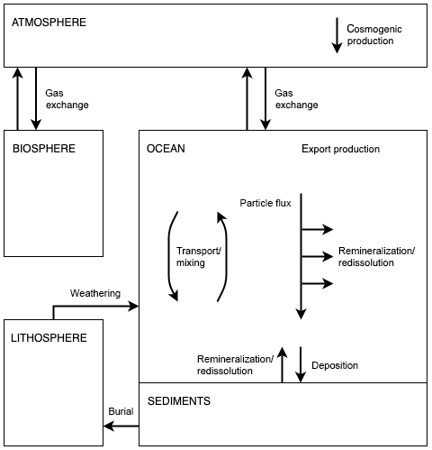
Figure 2Schematic diagram of the Bern3D carbon cycle model. The fully coupled model includes the major global carbon reservoirs (atmosphere, terrestrial biosphere, ocean, and sediments) and the exchange fluxes between them. Biogeochemical processes, namely air–sea gas exchange, biological export production, and particle flux through the water column, are parameterized by refined OCMIP-2 formulations. Details concerning the model are provided in Sect. 2 and Appendix A.
Radiocarbon measurements are generally reported as Δ14C, i.e., the ratio of 14C to total carbon C relative to that of the 1950 CE atmosphere, with a correction applied for fractionation effects, e.g., due to gas exchange and photosynthesis (see Stuiver and Polach, 1977). In this model study, Δ14C is treated as a diagnostic variable using the two-tracer approach of OCMIP-2. Rather than treating the 14C∕C ratio as a single tracer, fractionation-corrected 14C is carried independently from the carbon tracer. The modeled 14C concentration is normalized by the standard ratio of the preindustrial atmosphere (; Orr et al., 2017) in order to minimize the numerical error of carrying very small numbers. For comparison to observations, Δ14C is calculated from the normalized and fractionation-corrected modeled 14C concentration as follows:
where 14r′ is the ratio of 14C∕C in either atmospheric CO2 or oceanic DIC divided by 14rstd, depending on the reservoir being considered. The approach taken to simulate atmospheric 14CO2 is analogous to the approach used for CO2, except that the equation includes the terms due to atmospheric production and radioactive decay. For simulations in which the sediment model is active, the oceanic DIC tracer sees a constant input from terrestrial weathering, whereas there is no weathering input of DI14C to the ocean (see Appendix A for more details).
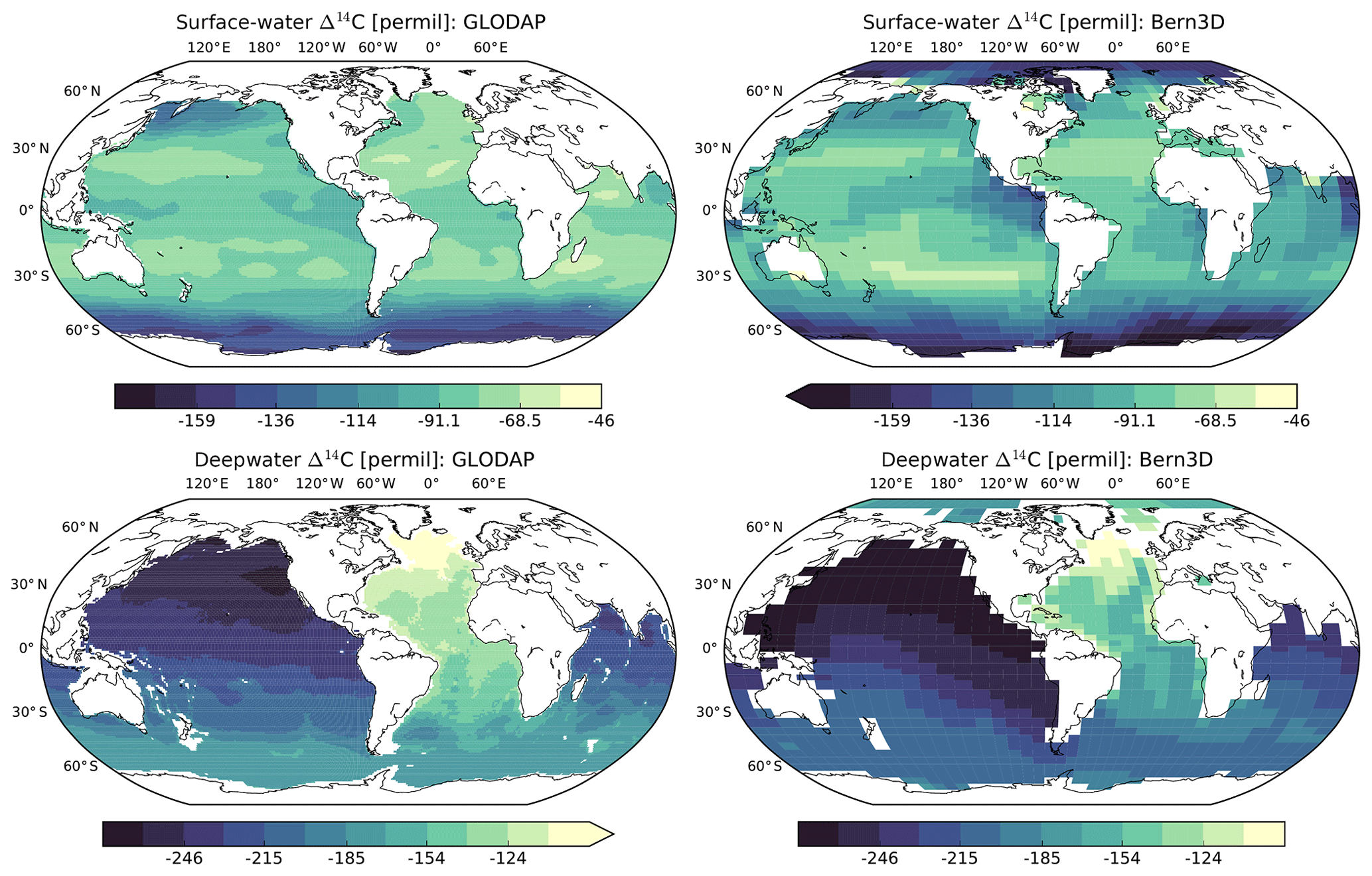
Figure 3Steady-state distribution of Δ14C in the surface (<100 m) and deep (>1500 m) ocean for the preindustrial control run (right) compared to the distribution of Δ14C based on the Global Ocean Data Analysis Project (GLODAP).
In the preindustrial spin-up simulation needed to initialize the Bern3D model, atmospheric CO2 is held constant at 278.05 ppm and Δ14Catm at 0 ‰. During this integration time the ocean inventories of carbon and 14C adjust to the forcing fields. The resulting changes after >50 000 years of integration are negligibly small. Figure 3 shows the steady-state Δ14C distribution in the surface (<100 m) and deep (>1500 m) ocean for the preindustrial control run. The large-scale distribution of modeled oceanic Δ14C broadly resembles the observed pattern in the Global Ocean Data Analysis Project (GLODAP; Key et al., 2004). That final state (i.e., the end of the preindustrial spin-up) is used to diagnose the 14C production rate for the preindustrial atmosphere such that the rate of 14C production is balanced by radioactive decay and the net fluxes out of the atmosphere. For transient simulations, an adjustable scale factor is applied to the preindustrial steady-state value of 443.9 mol14C yr−1 (1.66 ) in order to account for production changes induced by solar and/or geomagnetic modulation. These production changes are derived from, e.g., available reconstructions of the 14C production rate in relative units, as detailed in Sect. 2.5. Note the preindustrial spin-up results in steady-state values for weathering-derived inputs of DIC, Alk, P, and Si of 0.46 Gt C yr−1, 34.37 Tmol Alk yr−1, 0.17 Tmol P yr−1, and 6.67 Tmol Si yr−1, respectively. These terrestrial weathering rates were chosen to balance the sedimentation rates on the seafloor and are held fixed and constant throughout the simulations.
2.3 Model configurations
We focus in this paper on the response of Δ14Catm to changes in 14C production and the ocean carbon cycle. For a deeper mechanistic understanding of the driving processes, step response experiments are first performed (see Sect. 3.1). These simulations include perturbations of the steady-state 14C∕C distribution under preindustrial conditions. We investigate the impact of step changes in (1) the 14C production rate (“higher production” scenario), (2) wind stress and vertical diffusivity (“reduced deep ocean ventilation” scenario), and (3) the gas transfer velocity (“enhanced permanent sea ice cover” scenario). After a step change at time 0, the simulations are run to near equilibrium over a 50 000-year integration. The following model configurations and therefore exchanging carbon reservoirs are considered: atmosphere–ocean (OCN), atmosphere–ocean–land (OCN-LND), atmosphere–ocean–sediment (OCN-SED), and atmosphere–ocean–land–sediment (ALL).
Next we examine the influence of changes that are transient in nature. We simulate Δ14Catm over the full range of the 14C dating method (i.e., 50 to 0 ka) (see Sect. 3.2 and 3.3). These transient simulations are initialized at 70 ka using model configuration ALL and forced by reconstructed changes in 14C production (see Sect. 2.5) over a 70 000-year integration. The first 20 000 years of the integration are considered a spin-up. Although the full record is simulated, we focus our analysis on the millennial-scale variation in Δ14Catm before incipient deglaciation at ∼18 ka. Eight model runs are carried out for each production rate reconstruction using different combinations of forcing fields and parameter values as described next.
2.4 Carbon cycle scenarios
In our transient simulations with the Bern3D model, eight scenarios based on different assumptions about the global carbon cycle are considered, the details of which are summarized in Table 1. The goal is to investigate the extent to which changes in the ocean carbon cycle could explain high glacial Δ14Catm levels given available reconstructions of past changes in 14C production. We therefore consider a wide range of carbon cycle scenarios, including some extreme cases. A note of caution: because millennial-scale Δ14Catm variations during the last glacial are what we are interested in, we do not attempt to reproduce abrupt climate perturbations such as Dansgaard–Oeschger warming events in the model runs.
Table 1Summary of model scenarios considered in this study. Initial conditions refer to the boundary conditions used for the precursor spin-up simulation needed to initialize the transient simulation. These correspond either to preindustrial (PI) or last glacial conditions. The paleoclimate forcing fields, i.e., Orb-GHG-Ice, are reconstructed changes in orbital parameters (Berger, 1978), greenhouse gas radiative forcing based on reconstructed atmospheric greenhouse gas histories (Köhler et al., 2017), and varying ice sheet extent scaled using the global benthic δ18O stack of Lisiecki and Stern (2016). Numbers refer to the scale factor values applied to the tunable model parameters τ (wind stress scale factor), KV (vertical diffusivity), kw (gas transfer velocity), rr (CaCO3-to-POC export ratio), and ℓPOC (POC remineralization length scale) at the Last Glacial Maximum (LGM). These values were chosen in order to achieve an atmospheric CO2 concentration close to the LGM level and are varied over time using the global benthic δ18O stack. See Roth et al. (2014) for the Bern3D model parameter set. In all scenarios, the fully coupled model configuration, including the major global carbon reservoirs (atmosphere, terrestrial biosphere, ocean, and sediments), is used.
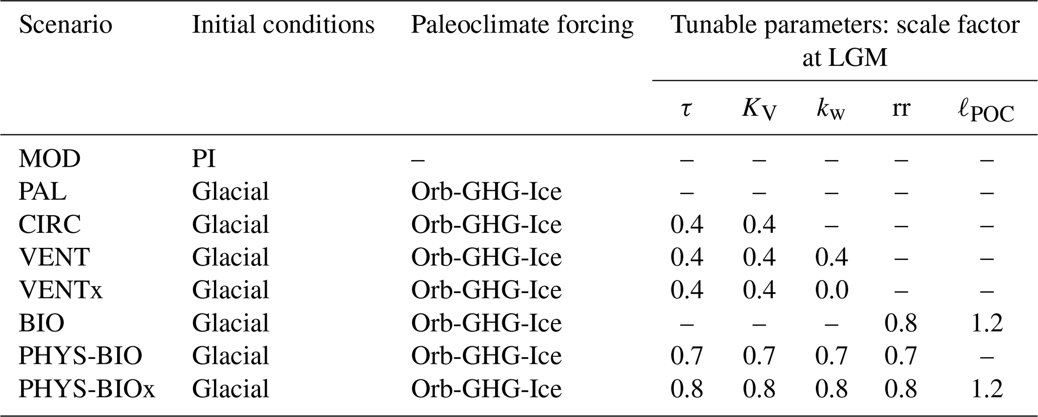
In the first scenario (MOD), the model is run with fixed preindustrial boundary conditions for the Earth's orbital parameters, radiative forcing due to well-mixed greenhouse gases, and ice sheet extent. As a consequence, atmospheric CO2 remains approximately constant at the preindustrial level of 278.05 ppm over the simulation. The second scenario (PAL) considers reasonably well-known climate forcing over the last glacial–interglacial cycle. Simulations under this scenario are initialized with output from a previous spin-up simulation forced by glacial boundary conditions with respect to orbital parameters (Berger, 1978), ice sheet extent (see below), and greenhouse gas radiative forcing based on the smoothed dataset of atmospheric greenhouse gases by Köhler et al. (2017) as constructed from the original data of Ahn and Brook (2014), Ahn et al. (2012), Bauska et al. (2015), Bereiter et al. (2012), Buizert et al. (2015), Dlugokencky et al. (2016), Lourantou et al. (2010), Lüthi et al. (2010), MacFarling-Meure et al. (2006), Marcott et al. (2014), Monnin et al. (2001, 2004), Rubino et al. (2013), Schneider et al. (2013), and Sigl et al. (2016). In simulations under PAL, the model is integrated until 0 ka following the reconstructed histories of orbital forcing, ice sheets, and radiative forcing due to greenhouse gases. Ice sheets for the preindustrial and Last Glacial Maximum (LGM) states are taken from Peltier (1994) and linearly scaled using the global benthic δ18O stack of Lisiecki and Stern (2016), which is a global ice volume proxy. Changes in the albedo, salinity, and latent heat flux associated with the ice sheet buildup or melting are also taken into account (Ritz et al., 2011). Note that, although the radiative forcing for CO2 is prescribed, the atmospheric CO2 concentration is allowed to evolve freely, except in the simulations described in Sect. 2.5.
Model scenario PAL appears to still be missing an important process or feedback for atmospheric CO2, as it cannot reproduce the observed low glacial CO2 level without invoking additional changes (see, e.g., Tschumi et al., 2011; Menviel et al., 2012; Roth and Joos, 2013; Jeltsch-Thömmes et al., 2019). Variations in atmospheric CO2 govern how fast Δ14C signatures are passed between the atmosphere and ocean. Gross fluxes of 14C between the atmosphere and ocean, and vice versa, scale with atmospheric pCO2 and its 14C∕C ratio. It is therefore important to reproduce low glacial atmospheric CO2 concentrations in at least some of the model scenarios, thereby capturing the influence of temporal changes in CO2 on the air–sea exchange of 14C. In this study, we consider six scenarios that invoke additional changes to force the model toward the observed low glacial CO2 concentration. In addition to the PAL forcing, a time-varying scale factor F(t) is applied to some combination of tunable model parameters: wind stress scale factor τ, vertical diffusivity KV, gas transfer velocity kw, CaCO3-to-particulate organic carbon (POC) export ratio (rr), and POC remineralization length scale ℓPOC. For the preindustrial period, the value of F(t) is fixed at 1, whereas the theoretical LGM value was chosen in order to achieve an atmospheric CO2 concentration close to the LGM level of ∼190 ppm (see Table 1), as determined by sensitivity experiments. Note that the same values of F(t) apply to any of the model parameters considered in a given scenario. To obtain intermediate values, F(t) is linearly scaled using the global benthic δ18O stack (see Fig. 1). For the spin-up needed to initialize these simulations, the glacial spin-up simulation of PAL was integrated for 50 000 model years, with tunable parameters adjusted to their appropriate glacial values. Atmospheric CO2 drawdown of up to ∼100 ppm is achieved over this 50 000-year integration. From that final spun-up state, the model is run forward in time until 0 ka with PAL and F(t) forcing.
The first of these scenarios (CIRC) allows us to test the sensitivity of the model results with respect to changes in ocean circulation. Tunable model parameters τ and KV were reduced to 40 % of their preindustrial values throughout the global ocean during the LGM (i.e., ). Such a drastic change in the wind stress field is not realistic. Rather, these changes should be viewed as “tuning knobs” that force the ocean model into a poorly ventilated state with an “older” ideal age and 14C-depleted deep waters, as suggested for the glacial ocean (e.g., Sarnthein et al., 2013; Skinner et al., 2017). In the model's implementation, a change in wind stress does not affect the gas transfer velocity kw, unlike in the real ocean where changes in wind stress and wind speed act together. The influence of a change in air–sea exchange efficiency on the model results was investigated in a second scenario (VENT) in which kw is reduced in the model's north (>60∘ N) and south (>48∘ S) polar areas in addition to global reductions of τ and KV (). A 60 % reduction of kw is unlikely to be correct but is a straightforward way to reduce the model's gas exchange efficiency. In the third scenario (VENTx), reduction of polar kw to 0 % of its preindustrial value was tested (; ). Here, kw remains fixed at 0 % during the last glacial and is adjusted to its preindustrial value via a linear ramp across the last glacial termination (∼18 to 11 ka). In this scenario, sea ice would permanently cover 100 % of the Southern Ocean during the last glacial, which is not supported by the sea ice reconstructions of Gersonde et al. (2005) and Allen et al. (2011), and also the high-latitude (>60∘ N) North Atlantic and Arctic Ocean, for which there is some evidence (Müller and Stein, 2014; Hoff et al., 2016).
We end by investigating the sensitivity of the model results to changes in the parameters controlling the export production of CaCO3 and the water column remineralization of POC. Model scenario BIO considers changes in the CaCO3-to-POC export ratio (and thus also the CaCO3-to-POC rain ratio; Archer and Maier-Reimer, 1994) (Frr=0.8) and POC remineralization length scale (Roth et al., 2014) (). These changes impact the global carbon cycle by influencing the vertical gradients of DIC, Alk, and nutrients in the water column. A change in the fluxes of POC and CaCO3 to the seafloor drives a change in the magnitude of their removal by sedimentation on the seafloor. A modest reduction in the export ratio during the last glacial is compatible with reconstructed variations in carbonate ion concentrations (Jeltsch-Thömmes et al., 2019). How the depth of POC remineralization changed over time is still unknown. The last two scenarios consider the combined effect of physical and biogeochemical changes: PHYS-BIO () and PHYS-BIOx (; ).
2.5 Measurement- and model-based reconstruction of 14C production
Our ability to attribute past changes in Δ14Catm to climate-related changes in the ocean carbon cycle is limited by our ability to reconstruct a precise and accurate history of the 14C production rate. Past changes in 14C production can be estimated from geomagnetic field reconstructions and from 10Be measurements in polar ice cores. For ice-core 10Be-based estimates, we use the ice-core radionuclide stack of Adolphi et al. (2018), which is based on 36Cl data from the GRIP ice core (Baumgartner et al., 1998) and on 10Be data from the GRIP (Yiou et al., 1997; Baumgartner et al., 1997; Wagner et al., 2001; Muscheler et al., 2004; Adolphi et al., 2014) and GISP2 (Finkel and Nishiizumi, 1997) ice cores. It also includes 10Be data from the NGRIP, EDML, EDC, and Vostok ice cores around the Laschamp geomagnetic excursion (Raisbeck et al., 2017). It has been extended to the present using the 10Be stack of Muscheler et al. (2016). All ice cores were first placed on the same timescale (GICC05) before 10Be fluxes were calculated. This 70 000-year 10Be stack provides relative changes in 14C production rates under the assumption that 14C and 10Be production rates are directly proportional, as indicated by the most recent production rate models (e.g., Herbst et al., 2017).
For paleointensity-based estimates, we employ (1) the North Atlantic Paleointensity Stack, or NAPIS, by Laj et al. (2000) as extended by Laj et al. (2002), (2) the Global Paleointensity Stack, or GLOPIS, by Laj et al. (2004), (3) a high-resolution paleointensity stack from the Black Sea (Nowaczyk et al., 2013), and (4) a paleointensity stack from Iberian Margin sediments (Channell et al., 2018). In principle, stacks of widely distributed cores (NAPIS and GLOPIS) are expected to yield a better representation of the global geomagnetic dipole moment, whereas the paleointensity stacks from the Black Sea and the Iberian Margin avoid some of the problems associated with coring disturbances. The four different paleointensity stacks were converted to 14C production rates using the production rate model of Herbst et al. (2017), the local interstellar spectrum of Potgieter et al. (2014), and assuming a constant solar modulation potential of 630 MeV.
An alternative approach to estimating the 14C production rate is to combine an atmospheric radiocarbon budget with a prognostic carbon cycle model. Here simulations are performed with the Bern3D model and forced by reconstructed changes in Δ14Catm and CO2, as well as reconstructed and hypothetical carbon cycle changes, over the last 50 kyr. Both the IntCal13 calibration curve (Reimer et al., 2013) and the recent Hulu Cave Δ14Catm dataset (Cheng et al., 2018) are used. Note that although the forthcoming IntCal20 calibration curve (Reimer et al., 2020) will be the new standard atmospheric radiocarbon record for the last 55 000 years, essentially all data underlying IntCal20 before 13.9 ka are tied to the Hulu Cave dataset, either via timescales (Lake Suigetsu plant macrofossil data) or marine reservoir corrections (marine records). Hence, the IntCal20 and Hulu Cave Δ14Catm records are very similar, and using IntCal20 would not impact our conclusions.
The 14C production rate Q is calculated each model year from the air–sea 14CO2 flux (Fas), the atmosphere–land 14CO2 flux (Fab), the loss of 14C due to radioactive decay, and the change () in the atmospheric 14C inventory (Ia):
where λ is the radioactive decay constant for 14C, i.e., yr−1. The radioactive decay term λIa and the change in inventory follow the reconstructed Δ14Catm and CO2 records, whereas Fas and Fab are explicitly computed by the model. The Fas term depends strongly on the carbon cycle scenario under consideration (see Sect. 2.4 and Table 1). For comparison with other reconstructions, Q is converted into a relative value by normalizing it by the preindustrial value.
3.1 Atmospheric Δ14C response to step changes
We use step changes in the 14C production rate, and in selected carbon cycle parameters, to gain insight into the characteristic magnitude and timescale of the corresponding Δ14Catm changes (Fig. 4). Besides variations of the production rate, changes in ocean circulation and air–sea gas exchange are considered the most important factors affecting Δ14Catm. Their effect on Δ14Catm can be understood in terms of their effect on the reservoir sizes involved in the global carbon cycle and on the exchange rates between the reservoirs. We investigate the relative importance of the major global carbon reservoirs (atmosphere, terrestrial biosphere, ocean, and sediments) by considering four different model configurations (see Sect. 2.3), with particular emphasis on the role of marine sediments.

Figure 4Response of atmospheric Δ14C to step changes in 14C production, followed by step changes in the tunable model parameters of the ocean carbon cycle. (a) 14C production Q is increased at time 0 from 100 % to 110 % of its preindustrial value (“higher production” scenario). (b) Wind stress scale factor τ and vertical diffusivity KV are decreased at time 0 from 100 % to 50 % of their preindustrial values (“reduced deep ocean ventilation” scenario). (c) Gas transfer velocity kw is decreased at time 0 from 100 % to 0 % of its preindustrial value at the North Pole (>60∘ N) and South Pole (>48∘ S; “enhanced permanent sea ice cover” scenario). Four model configurations are considered. The dark turquoise line shows the model results using the atmosphere–ocean (OCN) configuration, the light turquoise line is the atmosphere–ocean–land (OCN-LND) configuration, the light brown line is the atmosphere–ocean–sediment (OCN-SED) configuration, and the dark brown line is the atmosphere–ocean–land–sediment (ALL) configuration.
In model studies, the process of sedimentation (defined here as the difference between deposition and the remineralization and dissolution of material on the seafloor) is often neglected because it is a relatively minor flux. In the Bern3D model, sedimentation removes only about 0.46 Gt C yr−1 and 45.31 mol 14C yr−1 in the preindustrial steady state. Indeed, the interaction with the ocean sediments has little influence on the global mean value of oceanic Δ14C and therefore Δ14Catm, as long as the total oceanic amount of carbon remains approximately constant (Siegenthaler et al., 1980); however, this is not always true, particularly in the case of millennial-scale climate perturbations. This is demonstrated by the differences between the model runs with and without sediments (i.e., ALL vs. OCN-LND and OCN-SED vs. OCN) as shown in Fig. 4. The response of Δ14Catm to various perturbations depends on the magnitude of the change in the ocean carbon inventory, with a larger change achieved by considering the interaction with the ocean sediments and the imbalance between weathering and sedimentation (see Fig. 5e, f). In order to facilitate our discussion, we will make only direct comparisons between model runs ALL and OCN-LND, which both include the four-box terrestrial biosphere model. We note that the 14C exchange rate between the atmosphere and the terrestrial biosphere is only of minor importance for long timescales of millennia and more.
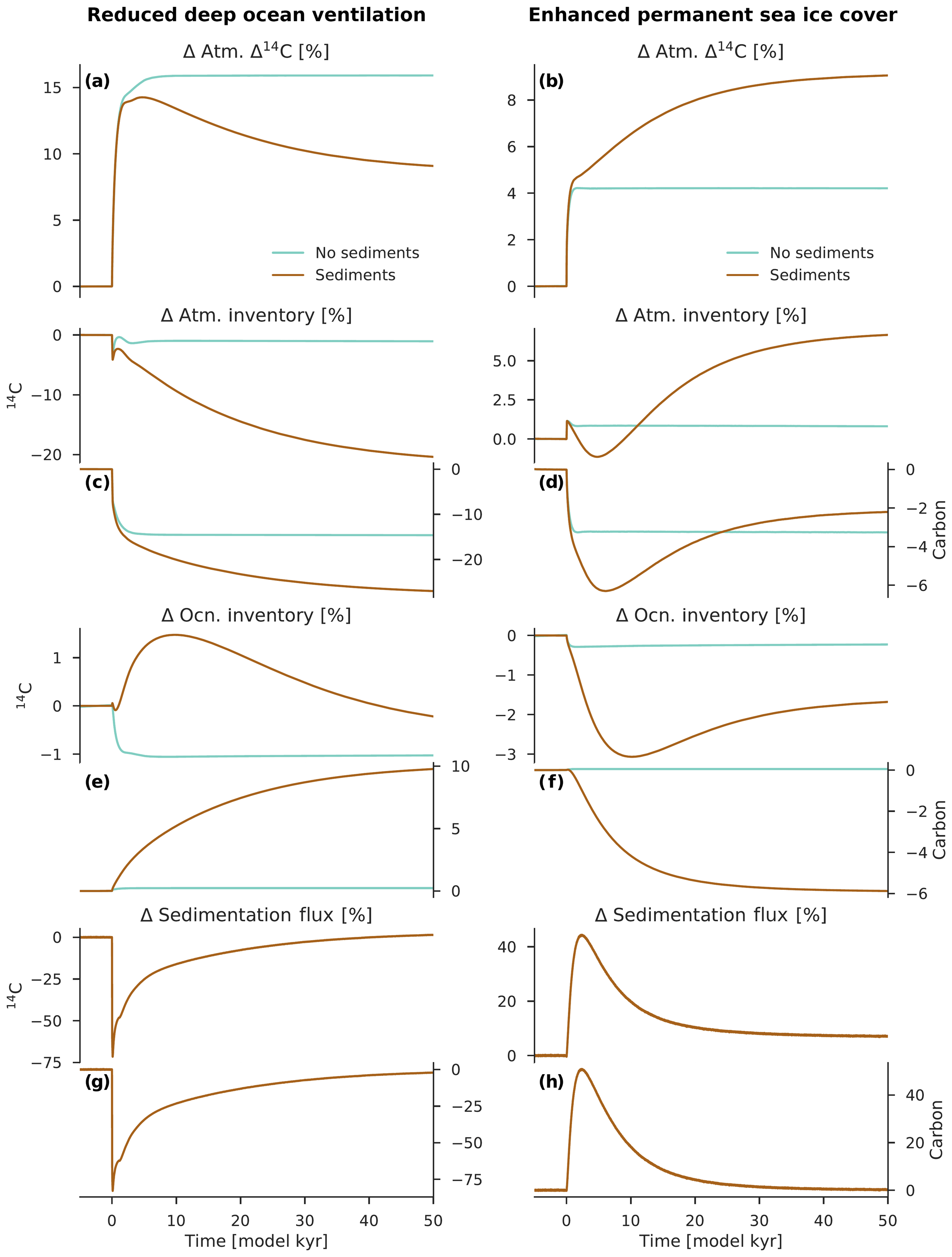
Figure 5Changes in carbon reservoir sizes and the sedimentation flux for the scenarios “reduced deep ocean ventilation” (a, c, e, g) and “enhanced permanent sea ice cover” (b, d, f, h). The change in atmospheric Δ14C is also shown (a, b). Anomalies are expressed here as differences relative to the preindustrial steady state (in percent). Turquoise lines show the model results using configuration OCN-LND (without sediments), and brown lines are configuration ALL (with sediments). The y axis on the left-hand side of each panel refers to changes in the 14C inventory, whereas the y axis on the right-hand side of each panel refers to changes in the carbon inventory or flux.
3.1.1 Change in 14C production
At steady state, the relative change in Δ14Catm is equal to the relative change in the 14C production rate, irrespective of the individual reservoirs considered. Figure 4 shows that Δ14Catm increases by about 100 ‰ (or 10 %) when the production rate is increased by 10 %. In model run ALL, Δ14Catm increases approximately exponentially to its new steady-state value with a characteristic time constant T of about 6170 years (i.e., % of the total change in Δ14Catm occurs within 6170 years). This e-folding timescale is close to the mean lifetime of 14C (∼8223 years), which is modulated by the time required for Δ14C to equilibrate between the atmosphere and the ocean (i.e., the timescale for deep ocean ventilation, of the order of hundreds of years to 1000 years or more). In the next section, we will investigate the effect of ocean carbon cycle processes on Δ14Catm.
Note that for simplicity, we investigated only step changes in atmospheric production, although in reality 14C production varies continuously over time due to changes in the solar and/or geomagnetic modulation of the cosmic radiation. This results in a non-steady-state value of Δ14Catm.
3.1.2 Change in ocean circulation
The exchange rate between the surface and deep ocean is mainly determined by physical transport and mixing processes. The overall effect of these processes is to transport 14C-enriched surface waters to the thermocline and deep ocean, where waters are typically 14C-depleted. In addition, the nutrient supply by transport and mixing plays an important role in determining the production and export of biogenic material from the surface ocean, constituting a second pathway for transporting 14C to the deep ocean.
In the Bern3D model, the tunable model parameters affecting the ventilation of the deep ocean include a scale factor τ for the wind stress field and vertical diffusivity KV. Figure 4 shows the Δ14Catm response after a sudden decrease in τ and KV by 50 %. Although a halving of τ and KV does not represent a realistic change, the resulting state of the ocean's large-scale overturning circulation can be interpreted in terms of the “ideal age” of water, which represents the average time since a water mass last made surface boundary contact. The new steady-state ideal age after a halving of τ and KV is almost 3 times greater than the preindustrial steady-state value (i.e., ∼1664 years vs. ∼613 years). This “aging” of the ocean is achieved through a weakening and shoaling of the global meridional overturning circulation, as evident from a moderate reduction in the meridional overturning stream function for the Indo-Pacific Ocean from about 14 to 9.5 Sv (1 Sv = 106 m3 s−1), and a very strong reduction from about 18 to 8 Sv in the Atlantic meridional overturning stream function, consistent with evidence for the glacial ocean. Here, as expected, the overall effect of deepwater aging is a stronger vertical Δ14C gradient in the water column and a subsequent increase in Δ14Catm. The exact nature of the Δ14Catm response, however, depends on the carbon reservoirs considered.
If the ocean sediment reservoir is neglected, the time required for Δ14Catm to adjust to step changes in τ and KV is relatively short. Δ14Catm increases rapidly to its new steady-state value of ∼159 ‰, with a time constant T of about 600 years. This increase in Δ14Catm can be explained by the fact that, owing to a weaker and shallower overturning circulation, a comparatively large amount of carbon is moved from the atmosphere to the ocean. More specifically, the atmospheric carbon inventory decreases by 14.6 %, whereas the atmospheric 14C inventory decreases by only 1.1 % (Fig. 5c). The 14C being produced in the atmosphere is therefore diluted by a smaller carbon inventory, increasing the atmospheric 14C∕C ratio; this asymmetry in the drawdown of CO2 and 14CO2 is what permits the increase in Δ14Catm. Since the ocean carbon inventory changes by only +0.2 %, the mean Δ14C value for the global ocean is nearly unaffected: a decrease of only ∼11 ‰ in the new steady state (Fig. 6g).
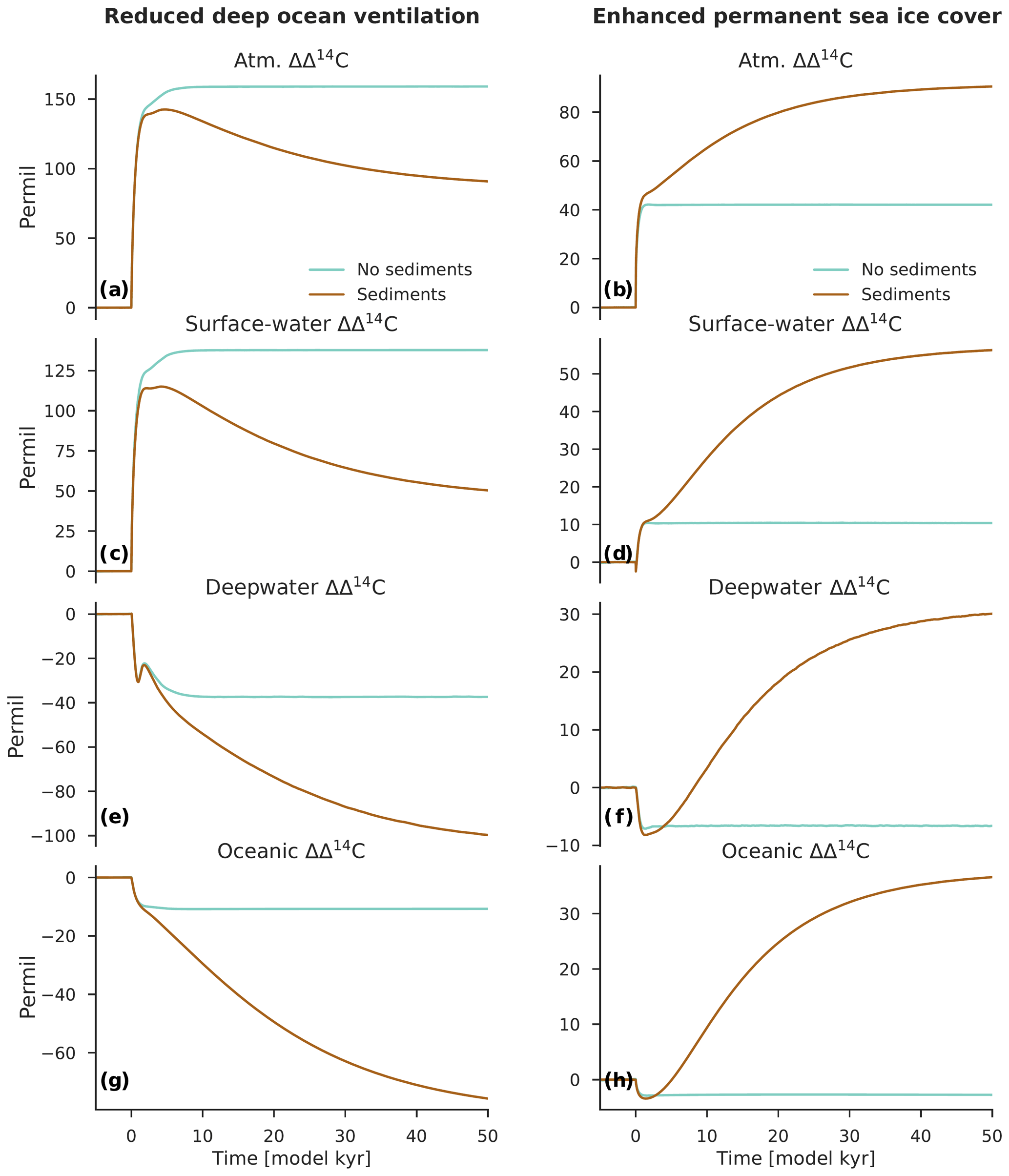
Figure 6Change in Δ14C for the atmosphere, surface ocean, deep ocean, and global ocean for the scenarios “reduced deep ocean ventilation” (a, c, e, g) and “enhanced permanent sea ice cover” (b, d, f, h). Anomalies are expressed here as differences relative to the preindustrial steady state (in per mill). Turquoise lines show the model results using configuration OCN-LND (without sediments), and brown lines are configuration ALL (with sediments).
In the model run in which the sediment model is active, there are two distinct time constants. A rapid increase in Δ14Catm occurs by ∼143 ‰ in the first few hundred years, then Δ14Catm gradually decreases to its final value of ∼91 ‰ after tens of thousands of years. Reduced deep ocean ventilation is again responsible for the rapid Δ14Catm change and the respective time constant ( years). The second time constant of ∼23 390 years is due to the relatively long time required for the ocean carbon inventory to adjust to the ocean-circulation-driven imbalance between weathering and sedimentation.
The process of ocean circulation interacts with the efficiency of the ocean's biological carbon pump via its impact on export production, ocean interior oxygen levels, and seawater carbonate chemistry and equilibria. This has important implications for the sedimentation of biogenic material on the seafloor and, on a timescale of tens of thousands of years, the total oceanic amount of carbon. Through this coupling of ocean circulation and seafloor sedimentation via the biological carbon pump, a halving of τ and KV leads to a 9.8 % increase in the ocean carbon inventory in the new steady state (Fig. 5e). Qualitatively, a reduction in the ocean's overturning circulation leads to a lower surface nutrient supply, which limits the production and export of biogenic material from the surface ocean. This, in turn, decreases the fluxes of POC and CaCO3 to the seafloor, with major consequences for the magnitude of their removal by sedimentation. At the same time, a constant input of DIC, Alk, and nutrients is added to the ocean from terrestrial weathering, which is no longer balanced by sedimentation on the seafloor (this is what permits a larger ocean carbon inventory). The overall effect is a gradual reduction of oceanic Δ14C by ∼76 ‰ (Fig. 6g), which dilutes the initial Δ14Catm peak by 52 ‰.
3.1.3 Change in gas transfer velocity
It takes about a decade for the isotopic ratios of carbon to equilibrate between the atmosphere and a ∼75 m thick surface mixed layer by air–sea gas exchange (Broecker and Peng, 1974). A consequence of this is that the surface ocean is undersaturated with respect to Δ14Catm (see Fig. 3). The choice of gas transfer velocity kw as a function of wind speed is critical for the efficiency of air–sea gas exchange. A reduction of kw corresponds to a higher resistance for gas transfer across the air–sea interface, which means that the 14C produced in the atmosphere escapes into the surface ocean at a slower rate. The effect of a lower kw is a larger air–sea gradient of Δ14C and higher Δ14Catm values. In contrast, the Δ14C value for the surface ocean is nearly unaffected so long as the ocean carbon inventory remains approximately constant, since the vertical gradient of Δ14C in the ocean is dominated by physical transport and mixing processes. Although the exact nature of the gas transfer velocity under glacial climate conditions remains unclear, kw represents a straightforward way to reduce the model's air–sea exchange efficiency due to theoretical changes in wind stress and sea ice.
Figure 4 shows how Δ14Catm responds to a perturbation in the gas transfer velocity. In the model run without sediments, the reduction of kw to 0 % of its preindustrial value in the model's north (>60∘ N) and south (>48∘ S) polar areas leads to a moderate increase in Δ14Catm in the new steady state. The amplitude of Δ14Catm change is ∼42 ‰, which is achieved with an e-folding timescale T of about 180 years. This relatively short time constant can be explained by the multidecadal timescale required for Δ14C to equilibrate between the model's atmosphere, upper ocean, and terrestrial biosphere. As shown in Fig. 6, the mean Δ14C values for the surface, deep, and global ocean in the new steady state are only slightly different from the preindustrial steady-state values, as expected from the fact that the ocean carbon inventory remains relatively stable.
Interestingly, if sediments are included in the model, the final value of Δ14Catm is much higher (∼91 ‰). In this case, a perturbation in kw leads to a very rapid initial increase in Δ14Catm (∼42 ‰) and a much slower subsequent increase in Δ14Catm (∼49 ‰). The latter has an e-folding timescale T of about 14 200 years. This slow doubling of the initial Δ14Catm increase is unexpected but can be explained by the fact that a reduction of kw also involves a reduction of air–sea O2 gas exchange in the deepwater formation regions, decreasing the oceanic oxygen that is available for transport to the deep ocean. This, in turn, implies lower oxygen concentrations in the water column and the sediment pore waters, decreasing the rate of POC remineralization in the sediments. Reducing this has the overall effect of enhancing POC sedimentation on the seafloor, causing the ocean carbon inventory to decrease. As shown in Fig. 5f, the total oceanic amount of carbon decreases by 5.9 % in the new steady state, resulting in elevated Δ14C values for the surface (+56 ‰), deep (+30 ‰), and global (+37 ‰) ocean as well as for the atmosphere (+91 ‰) (see Fig. 6). Note that the increase in Δ14Catm is not accompanied by a significant change in the atmospheric carbon inventory, which decreases by only 2.2 % to 3.3 %. The air–sea equilibration timescale for CO2 by gas exchange is about 1 year for a ∼75 m thick surface mixed layer (Broecker and Peng, 1974), which is much smaller than the ventilation timescale for the deep ocean (on the order of several hundred years or more). One would therefore expect that the oceanic uptake of CO2 demonstrates only a very small response to changes in kw.
Overall, findings from these sensitivity experiments demonstrate that (1) the response of Δ14Catm to changes in the internal parameters of the ocean carbon cycle, in contrast to 14C production changes, depends strongly on whether or not the balance between terrestrial weathering and sedimentation on the seafloor is simulated, (2) the e-folding timescale for the initial adjustment of Δ14Catm to ocean carbon cycle changes, i.e., changes in ocean circulation and gas exchange, is shorter than that for production changes (i.e., ∼600 and ∼180 years vs. ∼6170 years), (3) air–sea gas exchange, in contrast to ocean circulation, has only a small effect on atmospheric CO2 given that gas exchange is not the rate-limiting step for oceanic CO2 uptake, and (4) on timescales of tens of thousands of years changes in the balance between weathering and sedimentation can potentially diminish (or elevate) the Δ14Catm value. This is new, important information for future paleoclimate simulations and suggests that changes in Δ14Catm may be overestimated (or underestimated) in models that do not simulate the interaction between seafloor sediments and the overlying water column.
3.2 Role of 14C production in past atmospheric Δ14C variability
We now consider the component of past Δ14Catm variability caused by production changes alone. Figure 7 shows the results of model runs using different reconstructions of the 14C production rate, as inferred from paleointensity data and from ice-core 10Be fluxes. The global carbon cycle is assumed to be constant and under preindustrial conditions for these simulations (i.e., scenario MOD is used). Our analysis is restricted to the glacial portion of the record (50 to 18 ka), in part because this is the time period that experiences the largest production changes and in part because we did not attempt to reproduce the ∼80 ppm change in atmospheric CO2 that occurred during the last glacial termination. As we have already noted, much research over the last decades has attempted to explain the observed glacial–interglacial variations in Δ14Catm and CO2, and this was not the goal of this study.
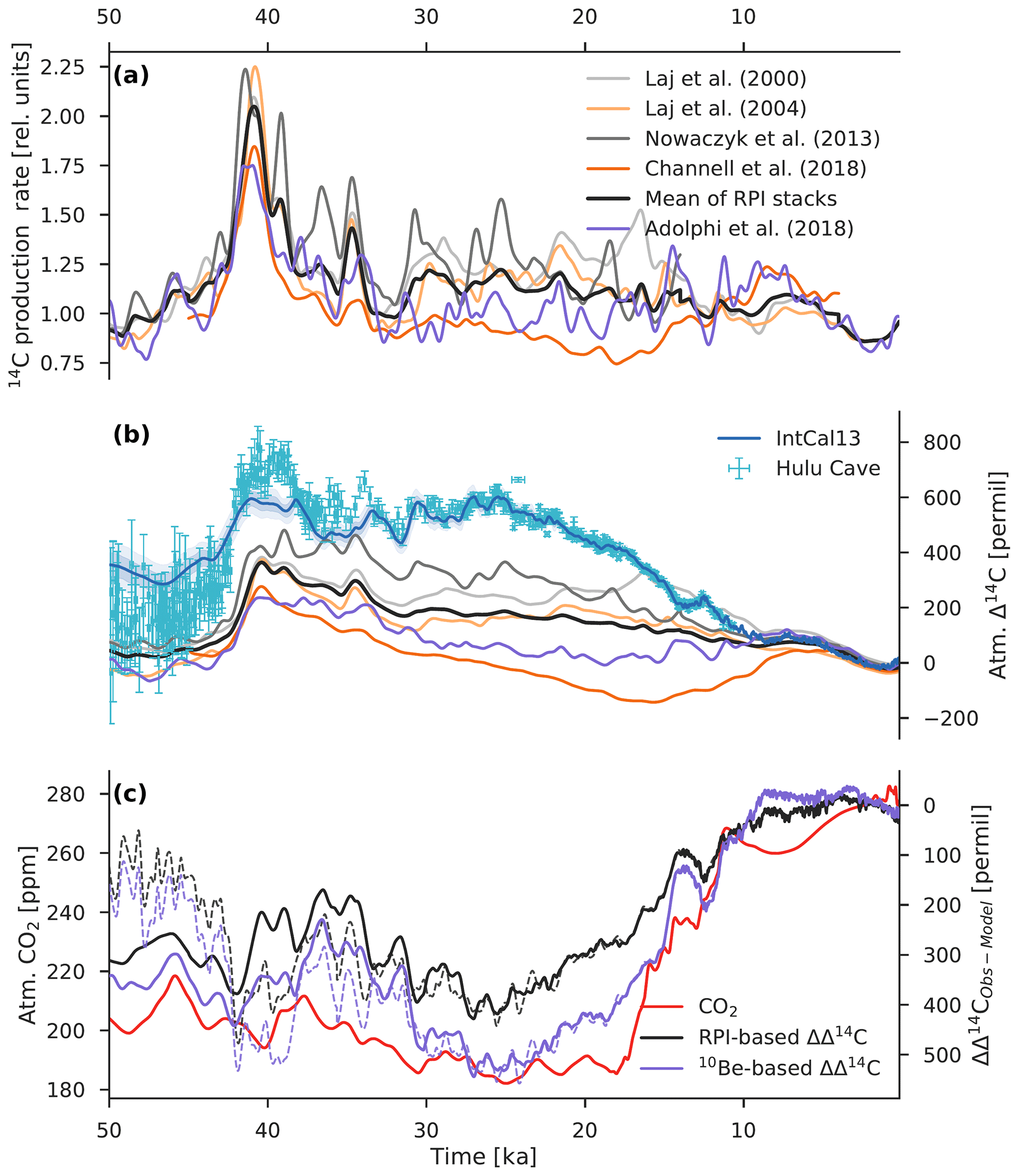
Figure 7Component of atmospheric Δ14C variability caused by production changes alone. (a) Relative 14C production rate as inferred from paleointensity data (gray) and from polar ice-core 10Be fluxes (purple). The heavy dark gray line is the mean paleointensity-based 14C production rate. (b) Modeled Δ14C records based only on 14C production changes compared with the reconstructed IntCal13 and Hulu Cave Δ14C records. The modeled records are given by scenario MOD that assumes a constant preindustrial carbon cycle. (c) Difference between reconstructed Δ14C and model-simulated Δ14C using averaged paleointensity data (RPI-based ΔΔ14C; gray) and the ice-core 10Be data of Adolphi et al. (2018) (10Be-based ΔΔ14C; purple) compared with the atmospheric CO2 record (red). Solid lines show the IntCal13–model difference, whereas dashed lines show the Hulu–model difference. The ΔΔ14C curve indicates changes in Δ14C that can be attributed to some combination of carbon cycle changes, uncertainties in the reconstruction of the 14C production rate, and uncertainties in the IntCal13 and Hulu Cave Δ14C records.
At first glance, the millennial-scale structure of model-simulated Δ14Catm is comparable to that of the reconstructions. These similarities appear to be highest for the oldest portion of the record, roughly before 30 ka. The model reproduces major features of the reconstructed Δ14Catm variability such as the large changes associated with the Laschamp (∼41 ka) and Mono Lake (∼34 ka) geomagnetic excursions. These two events are clearly expressed as distinct maxima in all model-simulated records. A more detailed comparison reveals a high correlation between the modeled and reconstructed Δ14Catm values between 50 and 33 ka. Of note is the better agreement with the new Hulu Cave Δ14Catm dataset compared to the IntCal13 calibration curve (i.e., Pearson correlation coefficient r of 0.96 vs. 0.91). This is likely due to the fact that the Laschamp excursion is smoothed and/or smeared out during the stacking process of the IntCal13 Δ14Catm datasets (Adolphi et al., 2018). The correlation between modeled and reconstructed Δ14Catm is much weaker during the millennia after the Mono Lake excursion (33 to 18 ka; r=0.52 to 0.64). While it is clear that much of the millennial-scale variation in Δ14Catm is driven by past changes in 14C production, the model fails to reproduce the glacial level of Δ14Catm and also does not capture the ∼15 000-year persistent elevation of Δ14Catm or the subsequent decrease in Δ14Catm after ∼25 ka.
The reconstructions suggest that the highest values of Δ14Catm occurred during the Laschamp excursion, with a maximum value of ∼595 ‰ at 41.1 ka found in the IntCal13 record. The Hulu Cave record indicates even higher values for the Laschamp event ( ‰ at 39.7 ka). In contrast, the model is able to simulate maximum Δ14Catm values of only ∼364 ‰ at 40.4 ka and ∼236 ‰ at 40.5 ka, as predicted by the paleointensity-based and ice-core 10Be-based production rate estimates, respectively. Although the model is unable to reproduce the reconstructed values of Δ14Catm, the modeled amplitude of the variation in Δ14Catm in response to the Laschamp event shows reasonable agreement with the reconstructed amplitude of Δ14Catm change found in the IntCal13 record (∼240 ‰). The Δ14Catm change predicted by paleointensity data has a maximal amplitude of about 320 ‰, whereas the ice-core 10Be data indicate a smaller amplitude (∼224 ‰). Note that the IntCal13 and model-simulated amplitudes of the Laschamp-related Δ14Catm change are about 2 times smaller than that observed in the Hulu Cave record (∼575 ‰), which is more likely to be correct.
Moving on to the full glacial record (50 to 18 ka), there are considerable discrepancies between reconstructed and modeled Δ14Catm (ΔΔ14C; see Fig. 7). The use of ice-core 10Be data to predict past changes in Δ14Catm results in the largest ΔΔ14C, with offsets between the records as high as ∼544 ‰ to 558 ‰ (root mean square error: RMSE=404 ‰ to 408 ‰). Model-simulated Δ14Catm given by paleointensity data varies widely between the four available reconstructions, yielding ΔΔ14C values of ∼325 ‰ to 639 ‰ (RMSE=206 ‰ to 455 ‰). Note that the upper limit of the paleointensity-based ΔΔ14C overlaps the ice-core 10Be-based ΔΔ14C. Given the uncertainties associated with the reconstruction of past changes in 14C production, accurate predictions of its contribution to past changes in Δ14Catm are challenging. Nonetheless, the substantial systematic offsets between the reconstructed and model-simulated Δ14Catm records after ∼33 ka point toward insufficiently high 14C production rates over this period of time. The question arises as to whether another factor besides geomagnetic modulation of the cosmic ray intensity was responsible for elevated glacial Δ14Catm levels. The effect of ocean carbon cycle changes on the evolution of Δ14Catm is considered next.
3.3 Carbon cycle contribution to high glacial atmospheric Δ14C levels
Here we investigate the magnitude and timing of the maximum possible Δ14Catm change during the last glacial period, obtained by running the Bern3D model with eight different carbon cycle scenarios (see Table 1). For the sake of clarity, we will discuss only the results of model runs using the mean paleointensity-based 14C production rate, though all available reconstructions were used. We emphasize that this is not a best-guess estimate of paleointensity-based 14C production. One should focus on the relative changes in Δ14Catm between model scenarios and how specific carbon cycle processes affect the glacial level of Δ14Catm.
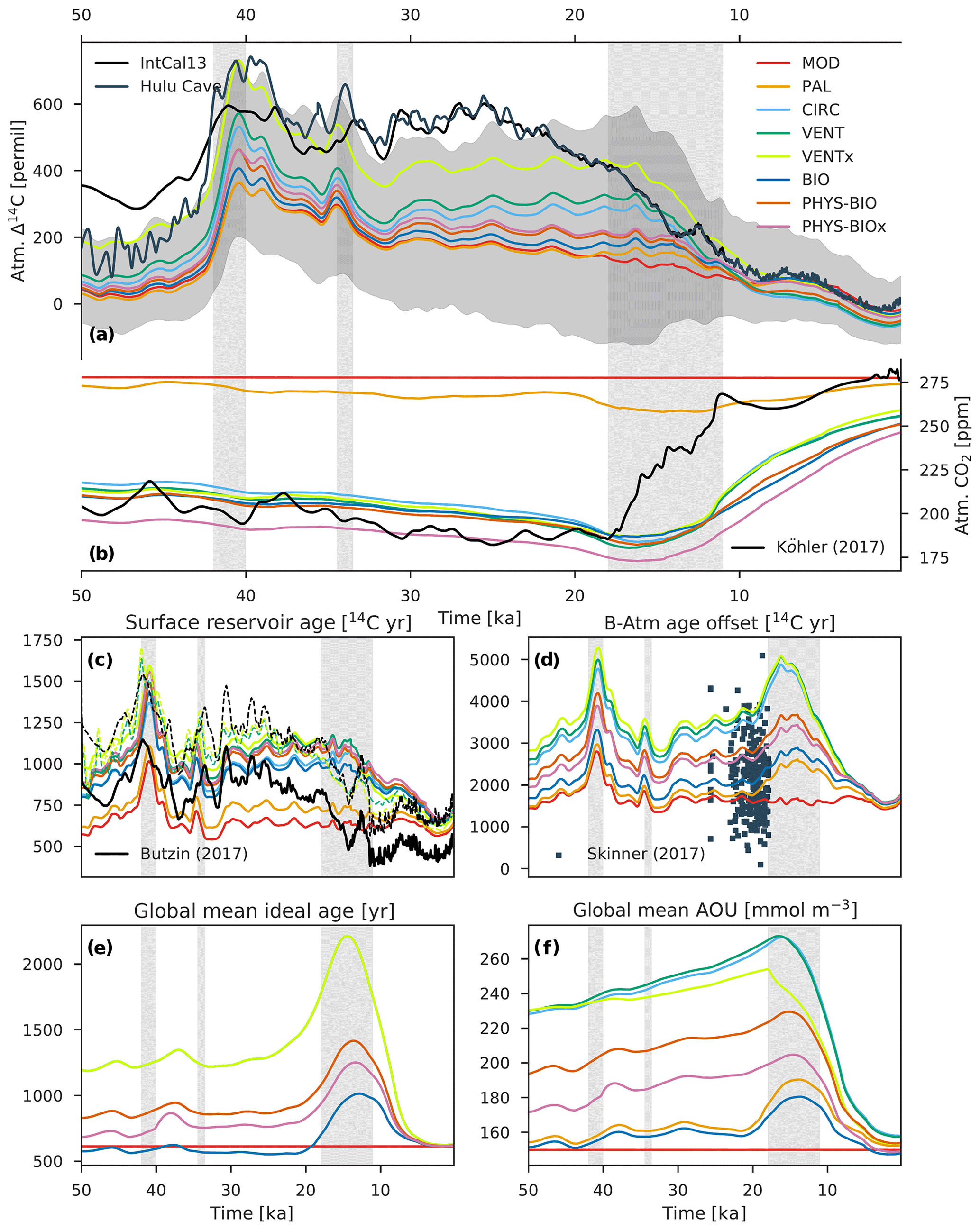
Figure 8Modeled records of atmospheric (a) Δ14C and (b) CO2 compared with their reconstructed histories (black and dark blue lines). Also shown are modeled records of the global average (c) surface reservoir age and (d) B-Atm 14C age offset compared with a recent compilation of LGM marine radiocarbon data (dark blue squares) by Skinner et al. (2017) and model-based surface reservoir age estimates between 50∘ N and 50∘ S (solid black line) and across all latitudes (dashed black line) from Butzin et al. (2017), as well as (e) ideal age and (f) apparent oxygen utilization (AOU). Colored lines show the results of model runs using the mean paleointensity-based 14C production rate and the eight different carbon cycle scenarios described in Sect. 2.4 and Table 1. The gray envelope in (a) shows the uncertainty (2σ) from all production rate reconstructions and carbon cycle scenarios, providing a bounded estimate of Δ14C change. The dashed colored lines in (c) show the surface reservoir age results from VENT and VENTx for which atmospheric Δ14C and CO2 are prescribed. Radiocarbon ventilation ages are expressed here as radiocarbon reservoir age offsets following Soulet et al. (2016), which are used extensively by the radiocarbon dating community.
Modeled 50 000-year records of Δ14Catm and CO2 as well as their reconstructed histories are shown in Fig. 8. In order to provide a basis for comparison of modeling efforts, the results of model run MOD (which assumes a constant preindustrial carbon cycle) are presented. The influence of ocean carbon cycle changes on Δ14Catm was tested in the other model runs. Interestingly, the forcing fields for model run PAL (orbital parameters, greenhouse gas radiative forcing, and ice sheet extent) have only a minimal impact on Δ14Catm. The PAL forcing fields also do not achieve sufficiently low glacial CO2 concentrations. Only a slight reduction of atmospheric CO2 by ∼20 ppm could be achieved, which unrealistically occurs during the last glacial termination (CO2=258.07 ppm at 14.6 ka). With hypothetical carbon cycle changes, the agreement between observed and modeled CO2 during the last glacial period is good (as by design), but the deglacial CO2 rise is lagged and ∼60 ppm too small at 11 ka. Since this study focuses on glacial Δ14Catm levels before incipient deglaciation at ∼18 ka, we will not discuss the lag any further.
Model simulation of high glacial Δ14Catm levels can be significantly improved by considering hypothetical carbon cycle changes in conjunction with PAL forcing. The amplitude of Δ14Catm change is highest for runs CIRC, VENT, and VENTx. This behavior is due to the fact that, owing to a reduction of τ, KV, and kw, strong vertical Δ14C gradients in the ocean and a large air–sea Δ14C gradient are established. As shown in Fig. 8, a more sluggish ventilation of deep waters is clearly expressed as an increase in the model ocean's global average ideal age and surface-water and deepwater reservoir ages; the latter two are calculated for the surface ocean and bottom water grid cells, respectively. These are equivalent to radiocarbon reservoir age offsets following Soulet et al. (2016). The deepwater reservoir age (i.e., B-Atm 14C age offset, or B-Atm) provides a measure of the radiocarbon disequilibrium between the deep ocean and the atmosphere, which arises due to the combined effect of air–sea gas exchange efficiency and the deep ocean ventilation rate, whereas the effect of upper ocean stratification and/or sea ice on air–sea gas exchange is particularly important for surface reservoir ages (i.e., surface R age) (Skinner et al., 2019).
Driven by a reduction in ocean circulation, model run CIRC predicts a substantial increase in B-Atm during the last glacial, which is defined here as 40 to 18 ka to avoid biasing global mean estimates toward Laschamp values. The global average glacial B-Atm predicted by CIRC is ∼3225 14C years, representing an increase in B-Atm of ∼1599 14C years relative to the preindustrial value of ∼ 1626 14C years. Model run VENT predicts a slightly larger increase in glacial B-Atm due to the inhibition of air–sea gas exchange. The “oldest” glacial waters are found in model run VENTx in which air–sea gas exchange is severely restricted, yielding an increase in B-Atm of ∼1912 14C years (glacial B-Atm ∼3538 14C years). The glacial B-Atm values given by runs CIRC, VENT, and VENTx, as well as the ∼717-year increase in ideal age during the last glacial relative to preindustrial, suggest that the glacial deep ocean was about 2 times older than its preindustrial counterpart. Comparison of our LGM B-Atm estimates (range of 3682 to 3962 14C years) with the compiled LGM marine radiocarbon data of Skinner et al. (2017) demonstrates that the carbon cycle scenarios are extreme, although it should be noted that Skinner et al. consider a wider depth range (∼500 to 5000 m) of the ocean than we do. Skinner et al. (2017) predict a global average LGM B-Atm value of ∼2048 14C years, an increase of ∼689 14C years relative to preindustrial. Turning our comparison to surface reservoir ages, we note that our global average LGM surface R age of ∼1132 14C years from runs VENT and VENTx is comparable to the ∼1241 14C years obtained by Skinner et al. (2017) for the LGM. The model-based estimates of surface R age from Butzin et al. (2017) indicate a much lower LGM value of ∼780 14C years and values ranging from 540 to 1250 14C years between 50 and 25 ka. Note that these estimates are based on model-simulated values between 50∘ N and 50∘ S. If the polar regions are included in the calculation (see Fig. 8c), their surface R-age estimates become comparable to our glacial values (range of 911 to 1354 14C years) and between about 34 and 22 ka can exceed them, even including those from model runs VENT and VENTx, unless Δ14Catm and CO2 are prescribed (dashed colored lines in Fig. 8c) as in the simulation by Butzin et al. (2017).
Indirect evidence for deepwater aging can be provided by the occurrence of depleted ocean interior oxygen levels due to the progressive consumption of dissolved oxygen during organic matter remineralization in the water column. This situation is amplified by the slow escape of accumulating remineralized carbon in the ocean interior (see, e.g., Skinner et al., 2017), leading to higher values of apparent oxygen utilization (). These two concepts (increased AOU and increased B-Atm) taken together signal a significant reduction in deep ocean ventilation characterized by a decrease in the exchange rate between younger (higher Δ14C) surface waters and older (14C-depleted), carbon-rich deep waters. Model runs CIRC, VENT, and VENTx do indeed indicate a large increase in AOU of about 95 mmol m−3 from its preindustrial value of ∼150 mmol m−3. The reason for this AOU increase is that a reduction of deep ocean ventilation permits enhanced accumulation of remineralized carbon in the ocean interior and therefore a more efficient biological carbon pump. Model runs BIO, PHYS-BIO, and PHYS-BIOx allow us to investigate the impact of other biological carbon pump changes on Δ14Catm and CO2 (i.e., changes in the CaCO3-to-POC export ratio and POC remineralization length scale). While these changes lead to an effective atmospheric CO2 drawdown mechanism, model results confirm that their effect on Δ14Catm is much less important (see Fig. 8).
Model run VENTx gives the best results with respect to glacial levels of Δ14Catm, with a maximum underestimation of ∼202 ‰ to 229 ‰ (RMSE=103 ‰ to 110 ‰) and a relatively good correlation (r=0.79 to 0.91). Only one model parameter was changed for run VENTx compared to runs CIRC and VENT, namely the polar gas transfer velocity kw was reduced to 0 % of its preindustrial value during the last glacial. In this extreme scenario, we assume that sea ice cover extended in the Northern Hemisphere as far south as 60∘ N and in the Southern Hemisphere as far north as 48∘ S, which is not supported by the reconstructions (Gersonde et al., 2005; Allen et al., 2011). Nonetheless, considering extreme assumptions about polar air–sea exchange efficiency under glacial climate conditions is interesting for two reasons: (1) a change in gas exchange hardly affects the atmospheric CO2 concentration, and (2) an additional change in Δ14Catm could possibly be achieved on a timescale of tens of thousands of years by changing the balance between weathering and sedimentation (see Sect. 3.1.3). This behavior has important implications for the glacial atmosphere, which is characterized by high Δ14C levels in conjunction with low but relatively stable CO2 concentrations. In contrast to a change in ocean circulation, air–sea gas exchange is a dedicated Δ14Catm “control knob” that can be invoked by models for a further increase in Δ14Catm without changing atmospheric CO2. Here, an additional increase in Δ14Catm of ∼130 ‰ relative to CIRC and VENT is achieved if gas exchange is permanently reduced to 0 % in the polar regions.
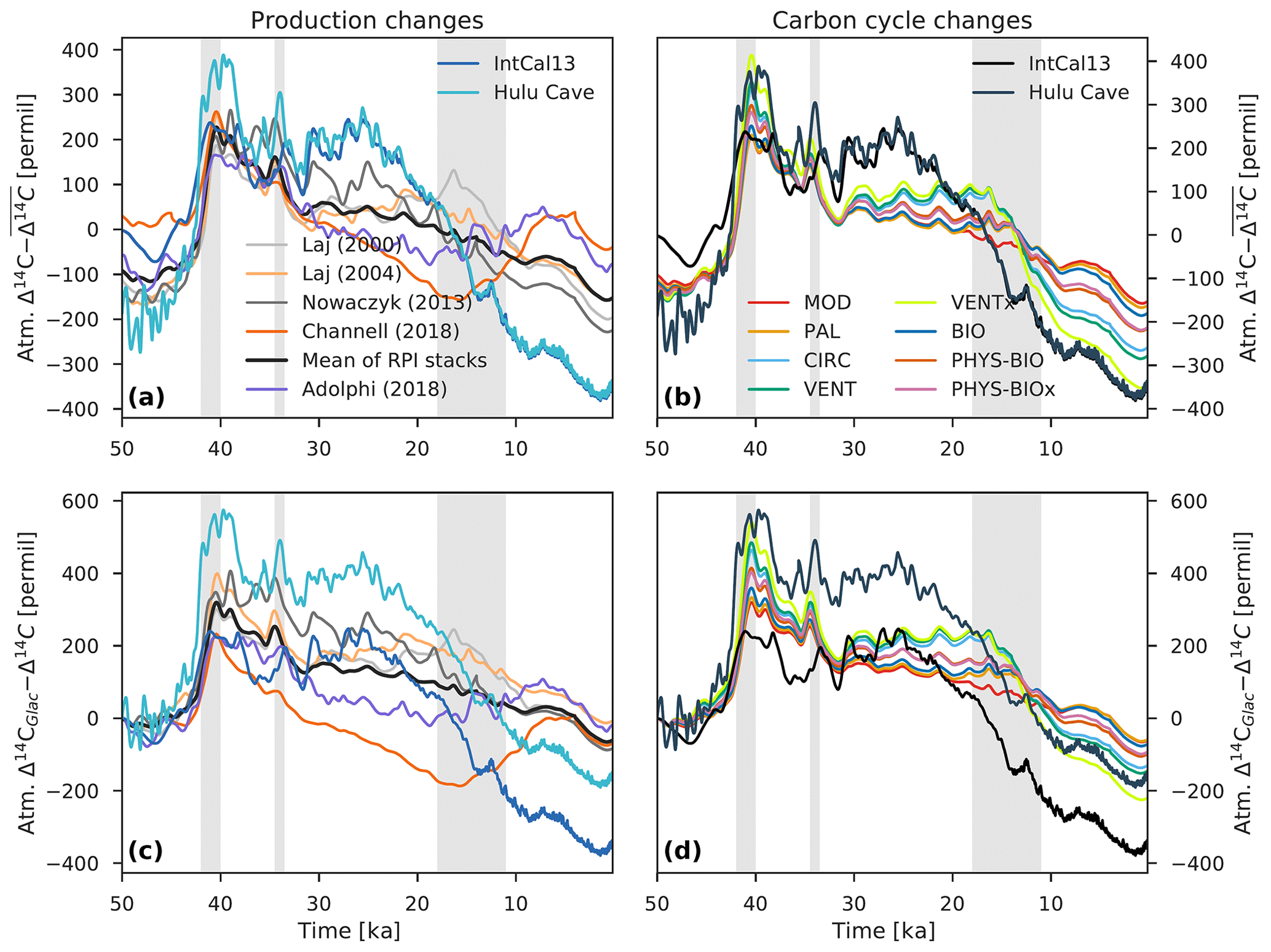
Figure 9Comparison of atmospheric Δ14C variability caused by changes in the ocean carbon cycle (b, d) with production-driven changes in atmospheric Δ14C using scenario MOD (a, c). For the analysis of carbon cycle changes, only the results of model runs using the mean paleointensity-based 14C production rate are shown. The Δ14C records in the upper panels (a, b) have been detrended by removing the mean, whereas the lower panels (c, d) show Δ14C anomalies expressed as differences relative to the Δ14C value at 50 ka. Three vertical light gray bars indicate the Laschamp (∼41 ka) and Mono Lake (∼34 ka) geomagnetic excursions, as well as the last glacial termination (∼18 to 11 ka).
While the modeled Δ14Catm values obtained by VENTx show rather good agreement with the reconstructions between 50 and 33 ka (r=0.92 to 0.96; RMSE=74 ‰ to 102 ‰), considerable discrepancies remain for the younger portion of the record. The analysis shown in Fig. 9 illustrates that even with extreme changes in the ocean carbon cycle it is very difficult to reproduce the reconstructed Δ14Catm values after ∼33 ka. During this period of time, VENTx underestimates Δ14Catm by up to ∼203 ‰ (RMSE=118 ‰ to 128 ‰) and is very poorly (r=0.1) correlated with the reconstructions, confirming that there are still considerable gaps in our understanding. Although it may be possible that permanent North Atlantic–Arctic and Antarctic sea ice cover extended to lower and higher latitudes than previously reconstructed, we conclude from our model study that even extreme assumptions about sea ice cover are insufficient to explain the elevated Δ14Catm levels after ∼33 ka. It appears instead that the glacial 14C production rate was higher than previously estimated and/or the reconstruction of glacial Δ14Catm levels is biased high. The older portion of the Δ14Catm record is based on data from archives other than tree rings (i.e., plant macrofossils, speleothems, corals, and foraminifera) (Reimer et al., 2013), providing, except for the Lake Suigetsu plant macrofossil data (Bronk Ramsey et al., 2012), only indirect measurements of Δ14Catm. Note that these data show uncertainty in calendar age that propagates into the estimation of past Δ14Catm levels.
Large uncertainties in the pre-Holocene 14C production rate also hamper our qualitative and quantitative interpretation of the Δ14Catm record. There is considerable disagreement between the available reconstructions of past changes in 14C production (Fig. 1). Paleointensity-based estimates typically predict higher 14C production rates than ice-core 10Be-based ones. An exception is the paleointensity stack from Channell et al. (2018), which predicts lower production rates. But, irrespective of the scatter, it is clear that all of the 14C production rate estimates are insufficiently high to explain the elevated Δ14Catm levels during the last glacial. Given the uncertainties in these estimates, it is very difficult to quantitatively describe the role of the ocean carbon cycle in determining the Δ14C and CO2 levels in the glacial atmosphere.
3.4 Reconstructing the 14C production rate by deconvolving the atmospheric Δ14C record
The unresolved discrepancy between reconstructed and model-simulated Δ14Catm raises the question of how the 14C production rate would have had to evolve to be consistent with the IntCal13 calibration curve or the new Hulu Cave Δ14Catm dataset. This question is addressed by deconvolving the Δ14Catm reconstruction over the last 50 kyr using the Bern3D carbon cycle model forced with reconstructed histories of Δ14Catm and CO2 (see Eq. 2). The carbon cycle scenarios described in Table 1, with the exception of MOD, are used in order to provide an estimate of the uncertainty associated with the model's glacial ocean carbon cycle. We note that the carbon cycle scenarios are not designed to capture the specific features of the last glacial termination, and therefore the results of the deconvolution over this time period must be considered very preliminary (and regarded as tentative). A detailed analysis of the Holocene 14C production rate is available in the literature (Roth and Joos, 2013). Finally, we consider the uncertainties associated with the older portion of the Δ14Catm record by deconvolving both the IntCal13 and Hulu Cave Δ14Catm records. Hulu Cave data overlap IntCal13 between ∼10.6 and 33.3 ka (Cheng et al., 2018), as expected from the fact that IntCal13 between 10.6 and 26.8 ka is based in part on Hulu Cave stalagmite H82 (Southon et al., 2012), whereas there are substantial offsets before ∼30 ka.
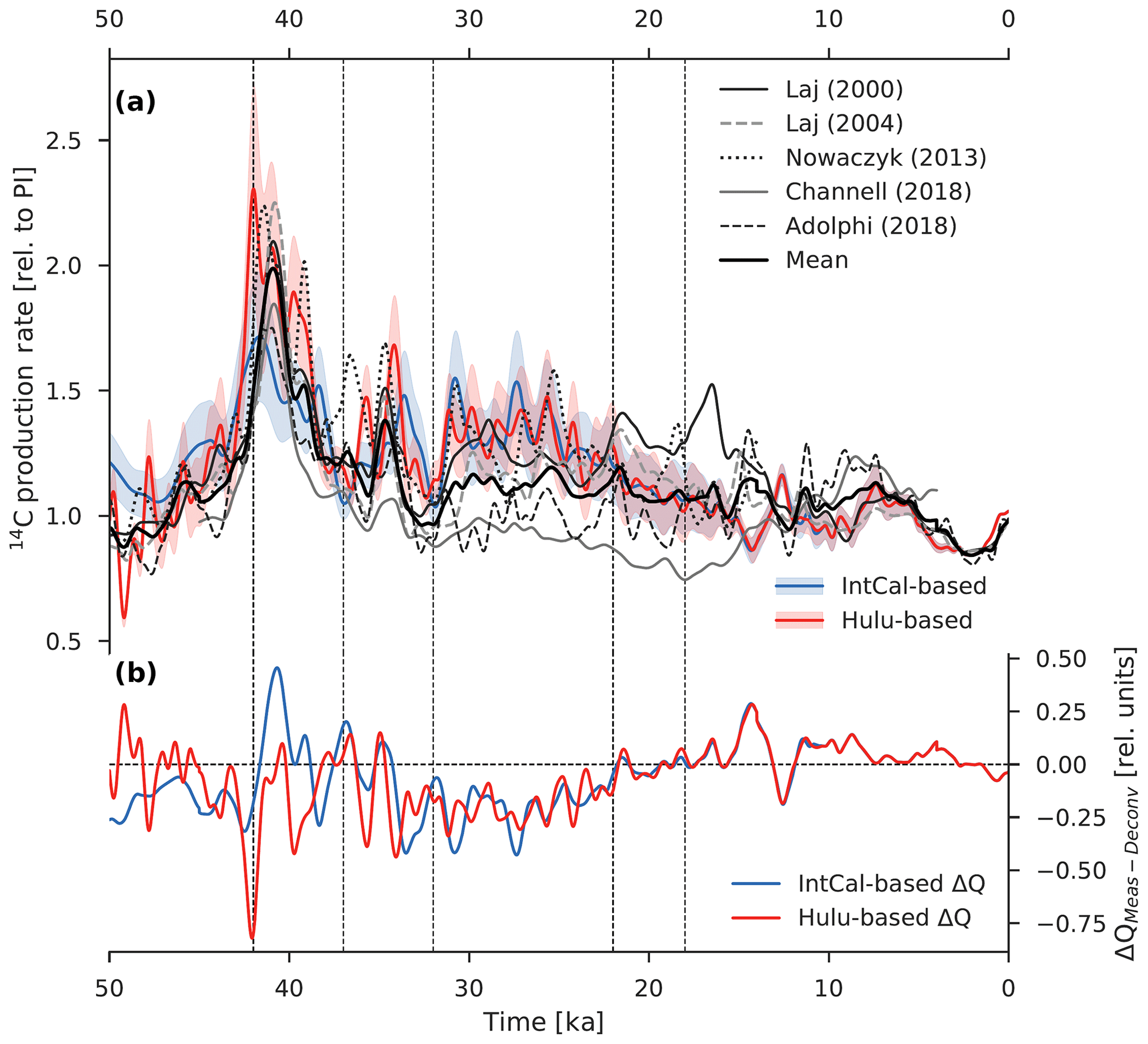
Figure 10Comparison of 14C production rate estimates inferred from a deconvolution of the atmospheric Δ14C record and from paleointensity and ice-core 10Be data. (a) 14C production rate calculated as the sum of the modeled air–sea and atmosphere–land 14CO2 fluxes as well as the reconstructed change in the atmospheric 14C inventory and loss of 14C due to radioactive decay (see Eq. 2). Model-based 14CO2 fluxes were obtained by forcing the Bern3D carbon cycle model with reconstructed variations in atmospheric Δ14C and CO2 as well as seven different carbon cycle scenarios. Results of model runs using the IntCal13 calibration curve are shown in the light blue envelope (2σ), whereas the light red envelope (2σ) shows the results from simulations using the composite Hulu Cave (10.6 to 50 ka) and IntCal13 (0 to 10.6 ka) Δ14C record. The heavy black line is the mean of five available production rate reconstructions: Laj et al. (2000, 2004), Nowaczyk et al. (2013), Channell et al. (2018), and Adolphi et al. (2018). (b) Difference between the mean of the measurement-based production rate estimates (heavy black line) and estimates based on the deconvolution of the IntCal13 (IntCal-based ΔQ; blue) and Hulu Cave (Hulu-based ΔQ; red) Δ14C data.
Figure 10 shows the new, model-based reconstruction of past changes in 14C production compared with available measurement-based reconstructions. Before the onset of the Laschamp excursion at ∼42 ka, production rates as inferred from the Hulu Cave record are near modern levels, whereas those obtained from the IntCal13 record are somewhat higher than modern. As expected, peak production occurs during the Laschamp event (∼42 to 40 ka), with the Hulu Cave dataset yielding the largest amplitude (factor of ∼2 greater than modern). The IntCal13 record predicts a smaller amplitude of ∼1.6 times the modern value. Both Δ14Catm records predict production minima at ∼37 ka (∼7 % higher than modern) and ∼32 ka (∼5 % higher than modern), interrupted by a prominent peak (factors of ∼1.5 and ∼1.4, respectively) during the Mono Lake geomagnetic excursion (∼34 ka), though the details of the timing and structure differ between the two records. Between 32 and 22 ka, model-based estimates of the 14C production rate are ∼1.3 times the modern value, which then decrease to around modern levels by HS1 (∼18 ka).
Table 2Production rate estimates in relative units inferred from three fundamentally different reconstruction methods: geomagnetic field data from marine sediments, 10Be and 36Cl measurements in polar ice cores, and model-based deconvolution of atmospheric Δ14C. Laj00, Laj04, Now13, and Chn18 refer to the paleointensity-based reconstructions of Laj et al. (2000), Laj et al. (2004), Nowaczyk et al. (2013), and Channell et al. (2018), respectively. Adp18 refers to the ice-core 10Be-based reconstruction of Adolphi et al. (2018). Int13 and Hul18 refer to the model-based reconstructions from this study using the IntCal13 calibration curve (Reimer et al., 2013) and the new Hulu Cave Δ14C dataset (Cheng et al., 2018). The bold numbers show the mean production rates during the last glacial (50 to 18 ka).
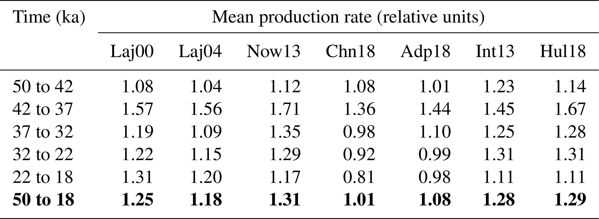
Model-based estimates of 14C production during the last glacial are typically higher than paleointensity-based and ice-core 10Be-based ones, as expected from Sect. 3.2. Between 32 and 22 ka, the deconvolutions of the IntCal13 and Hulu Cave Δ14Catm records give estimates that are about 17.5 % higher than the reconstructions. It is important to note that the differences between the reconstructions based on proxy data (i.e., paleointensity data and ice-core 10Be fluxes) are as large as the differences between our deconvolution results and the reconstructions (see Table 2). As shown in Fig. 11, it is extremely difficult to reconcile the discrepancies between measurement- and model-based 14C production on the basis of carbon cycle changes alone. Nonetheless, the fact remains that two independent estimates of the 14C production rate (i.e., estimates inferred from paleointensity data and from ice-core 10Be fluxes) show systematically lower rates than those obtained by our model-based deconvolution of Δ14Catm, in particular between 32 and 22 ka. The differences between the production rate results shown in Figs. 10–11 and Table 2 stem from various uncertainties that are discussed next.
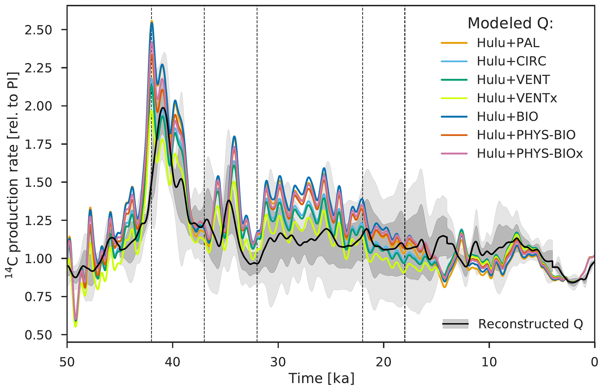
Figure 11Relative 14C production rate as inferred from the Bern3D model under seven carbon cycle scenarios (see Sect. 2.4). Estimates shown here are based on the composite Hulu Cave and IntCal13 Δ14C record. The black line is the mean of the five production rate reconstructions shown in Fig. 10; the gray envelope shows its uncertainty (2σ).
Uncertainties associated with the glacial ocean carbon cycle (Fig. 10, colored shading; Fig. 11, colored lines) are systematic in our approach. The deconvolutions, e.g., of the Hulu Cave Δ14Catm record, under different model scenarios are offset against one another, whereas the millennial-scale variability is maintained (see Fig. 11). We do not attempt to resolve uncertainties associated with Dansgaard–Oeschger warming events and related Antarctic and tropical climatic excursions in the model runs. Such climatic events may have influenced the atmospheric radiocarbon budget, but their influence on long-term variations in Δ14Catm, and therefore inferred production rates, is presumably limited. As may be expected, the lowest production rates (the lowest Fas values) are found in VENTx and the highest in scenarios PAL and BIO, mirroring the high and low glacial Δ14Catm levels achieved by these model scenarios as discussed in Sect. 3.3. Note that there is a large uncertainty in the model-based 14C production rate stemming from uncertainties associated with the reconstruction of past changes in Δ14Catm, in particular the older portion of the Δ14Catm record.
A shortcoming of paleointensity-based reconstructions of the 14C production rate is that they neglect changes in the solar modulation of the cosmic radiation. The solar modulation potential, which describes the impact of the solar magnetic field on isotope production, varied between 100 and 1200 MeV during the Holocene on decadal to centennial timescales, with a median value of approximately 565 MeV (Roth and Joos, 2013). A halving of the solar modulation potential (e.g., from 600 to 300 MeV) increases the 14C production rate by about 25 % for the modern geomagnetic field strength (Roth and Joos, 2013; see their Fig. 13). This sensitivity remains similar when changes in the strength of the geomagnetic field are limited as during the last ∼35 kyr (Muscheler and Heikkilä, 2011). A shift to lower solar modulation potential could have materialized if the sun spent on average more time in the postulated “grand minimum” mode (Usoskin et al., 2014) during the last glacial than during the Holocene. The sensitivity of isotope production to variations in solar modulation potential became large during the Laschamp event when the intensity of the geomagnetic field was close to zero, and changes in the solar modulation of the cosmic ray flux may have had a discernible impact on the high Δ14Catm levels found over this period. A reduction of the solar modulation potential from 600 to 0 MeV would double 14C production during times of zero geomagnetic field strength (Masarik and Beer, 2009). However, it is likely that changes in the solar modulation potential were insufficient to explain the discrepancy between paleointensity-based production rate estimates and the results of our deconvolution, in particular for the post-Laschamp period and for the reconstruction by Channell et al. (2018). Uncertainties associated with the paleointensity-based reconstructions also stem from uncertainties in estimating the age scales of the marine sediments and the geomagnetic field data.
The ice-core 10Be-based reconstruction of past changes in 14C production reflects, by definition, the combined influence of changes in the solar and geomagnetic modulation of the cosmic ray flux reaching the Earth. This method therefore avoids a fundamental shortcoming of reconstructions based on geomagnetic field data. The assumption is that the 10Be and 36Cl deposited on polar ice and measured in ice cores scales with the amount of cosmogenic isotopes in the atmosphere. A difficulty is to extrapolate measurements from a single location or a few locations to the global atmosphere. Changes in climate influence the atmospheric transport and deposition of 10Be as well as the snow accumulation rate, which affect the ice-core 10Be concentration (Elsässer et al., 2015). Furthermore, the sensitivity of 10Be in polar ice vs. the sensitivity of total production to magnetic field variations, or “polar bias”, is a point of debate, but atmospheric transport models (Heikkilä et al., 2009; Field et al., 2006) and data analyses (Bard et al., 1997; Adolphi and Muscheler, 2016; Adolphi et al., 2018) reach different conclusions about its existence and magnitude. If a polar bias was present, it would lead to an underestimation of the geomagnetic modulation of the ice-core 10Be flux, and therefore variations in the 10Be-based 14C production rate would also be underestimated. However, the mismatch of up to ∼544 ‰ to 558 ‰ between reconstructed and modeled 10Be-based Δ14Catm during the last glacial (see Fig. 7c) appears to be much too large to be reconciled by considering uncertainties in the polar bias alone. Furthermore, this mismatch with reconstructed Δ14Catm is qualitatively similar when using paleointensity-based 14C production rates that do not suffer from a polar bias (Fig. 7c).
Given the uncertainties associated with the proxy records, it may not be surprising that estimates of the 14C production rate for the last 50 kyr, as obtained by three fundamentally different methods (geomagnetic field data from marine sediments, 10Be and 36Cl measurements in polar ice cores, and model-based deconvolution of Δ14Catm), disagree with one another, typically by order 10 % and sometimes by up to 100 %. At the same time, it is intriguing that two independent estimates of the 14C production rate (i.e., estimates inferred from paleointensity and ice-core 10Be data) give values that are systematically lower than what is required to match the Δ14Catm reconstruction.
It is generally assumed that Δ14Catm is controlled by abiotic processes such as atmospheric 14C production, air–sea gas exchange, and ocean circulation and mixing. Here, results from sensitivity experiments with the Bern3D Earth system model of intermediate complexity suggest that Δ14Catm is potentially quite sensitive to the interaction with the ocean sediments on multimillennial timescales. This rather surprising result is due to the coupling of ocean circulation and the sedimentation of biogenic material on the seafloor via the biological carbon pump, which has important implications for the ocean carbon inventory. If the model's ocean carbon cycle is sufficiently perturbed, e.g., by changing the inputs or parameters controlling ocean circulation and/or gas exchange, the imbalance between weathering and sedimentation has a significant impact on the total oceanic amount of carbon. On timescales of tens of thousands of years this slow change in the ocean carbon inventory influences the partitioning of 14C∕C between the ocean and atmosphere and thus also oceanic Δ14C and Δ14Catm. This is important information for long-term climate studies and paleoclimate modeling efforts concerning Δ14Catm. Note that the representation of terrestrial weathering and seafloor sedimentation in the Bern3D model is necessarily simplified compared to reality. Nonetheless, a change in the ocean carbon inventory linked with the weathering–sedimentation balance should be discussed as one of the potentially important factors affecting Δ14Catm during the last glacial period.
The reason for the high Δ14C values exhibited by the glacial atmosphere is still not clear. In order to investigate potential mechanisms governing glacial Δ14Catm levels, the Bern3D model is again used as a tool. Results of model simulations forced only by production changes point out that none of the available reconstructions of the 14C production rate can explain the full amplitude of Δ14Catm change during the last glacial. In order to test the sensitivity of the model results with respect to the ocean carbon cycle state, various model parameters, i.e., different sets of physical and biogeochemical parameters, were “tuned” to match the glacial CO2 level. From this, we find that Δ14Catm is most sensitive to changes in physical model parameters, in particular those controlling ocean circulation and gas exchange. In order to achieve a Δ14Catm value close to the glacial level, the gas transfer velocity in the polar regions had to be reduced by 100 %. If interpreted as being due to a greater extent of permanent sea ice cover, a reduction in polar air–sea exchange efficiency is a possible explanation for high glacial Δ14Catm levels. Although this hypothesis is compelling, such a scenario is not supported by the proxy records of Antarctic sea ice cover (Gersonde et al., 2005; Allen et al., 2011) and the 13C∕12C ratio of atmospheric CO2 (Eggleston et al., 2016).
Atmospheric Δ14C that is modeled at any point in time reflects 14C production at that point, as well as the legacy of past production and carbon cycle changes. The question arises as to whether our conclusions are affected by unaccounted legacy effects, e.g., linked to the preindustrial spin-up simulation or model-diagnosed production rates. Transient simulations forced by reconstructed changes in 14C production (Sect. 3.2 and 3.3) are initialized at 70 ka, but their interpretation is restricted to the last 50 000 years of the integration to minimize legacy effects from model spin-up. Available reconstructions of the 14C production rate in relative units (Sect. 2.5) are applied as a scale factor to the preindustrial steady-state absolute value, which is diagnosed by running the Bern3D model to equilibrium under preindustrial boundary conditions. This approach represents an approximation and equilibrium conditions do not fully apply. Indeed, there is a mismatch between reconstructed and modeled Δ14Catm at the preindustrial (see Fig. 8a). This mismatch is on the order of a few percent or less, and adjusting the base level of production accordingly would not remove the large mismatch between reconstructed and modeled Δ14Catm during the last glacial. In addition, the uncertainty in the absolute value of the preindustrial production rate is on the order of 15 %, primarily due to the uncertainties in the preindustrial ocean radiocarbon inventory (see Roth and Joos, 2013, Sect. 3.2). This potential systematic bias, however, does not affect our conclusions as we consider normalized production rate changes (see Figs. 7, 10, and 11).
Before model-simulated Δ14Catm can be taken seriously, it must be demonstrated that the reconstruction of past changes in 14C production is reliable. There is, however, a substantial amount of scatter in the paleointensity-based and ice-core 10Be-based estimates of 14C production. Here we adopt an alternative approach to estimating the 14C production rate, which would indeed benefit from further constraints and lines of supporting evidence. Our deconvolution-based approach assumes that the 14C production rate can be derived from an atmospheric radiocarbon budget constructed using a prognostic carbon cycle model combined with the Δ14Catm record. Here, nonequilibrium effects are fully accounted for by transient simulations in which Δ14Catm and CO2 are prescribed following their reconstructed histories (Sect. 3.4). Yet, these simulations indicate that the discrepancy between measurement- and model-based estimates of the 14C production rate remains for the last glacial (Fig. 10b). This would suggest that unaccounted legacy effects do not significantly affect our conclusions. Our model results imply that the glacial 14C production rate as inferred from paleointensity data and ice-core 10Be fluxes may be underestimated by about 15 % between 32 and 22 ka, a time interval that appears to be an important piece of the glacial–interglacial Δ14Catm puzzle. Note that our model-based estimates are associated with uncertainties arising from the reconstruction of the older portion of the Δ14Catm record and from the model simulation of the glacial ocean carbon cycle (e.g., uncertainties in the glacial ocean circulation and air–sea CO2 fluxes). An improved understanding of the role of 14C production in past changes in Δ14Catm would open up the possibility of attributing model deficiencies to real changes in the ocean carbon cycle, but there is as yet no emerging single record of the 14C production rate.
Progress in several different areas may help to resolve the glacial–interglacial radiocarbon problem. Additional records of glacial Δ14Catm would help refine the older portion of the IntCal Δ14C record. Cosmogenic isotope production records may be improved, e.g., by refining estimates of ice accumulation, by developing a better understanding of 10Be transport and deposition during the glacial, by recovering additional long and continuous records from Antarctic ice cores and including marine 10Be records, and by obtaining additional geomagnetic field data. An expanded spatiotemporal observational coverage of Δ14C of DIC in the surface and deep ocean would help narrow the timescales of surface-to-deep transport and the air–sea equilibration of Δ14C, carbon, and nutrients, thereby guiding model-based analyses. Models should become more sophisticated and detailed in order to successfully reproduce the glacial–interglacial changes in carbon and radiocarbon by including exchange with sediments and the lithosphere, by better representing coastal processes, and by simulating a wide variety of paleo-proxies such as δ13C, Nd isotopes, carbonate ion concentration, lysocline evolution, and paleo-productivity proxies in a 3-D dynamic context for model evaluation. What is also missing are methods to quantify how the ocean carbon inventory, which codetermines the 14C∕C ratio and thus the Δ14C values in the ocean and atmosphere, has changed over the last 50 000 years. Ultimately, improved knowledge of 14C production during the last glacial and more robust constraints on the prevailing climate conditions (e.g., ocean circulation, sea ice cover, and wind speed) are necessary to elucidate the processes permitting mysteriously high Δ14C levels in the glacial atmosphere.
The physical core of the Bern3D model is based on the 3-D rigid-lid ocean model of Edwards et al. (1998) as updated by Edwards and Marsh (2005). The forcing fields for the model integration are monthly mean wind stress data taken from NCEP/NCAR (Kalnay et al., 1996). Diapycnal mixing is parameterized with a uniform vertical diffusivity KV of m s−1. The parameterization of eddy-induced transport is separated from that of isopycnal mixing using the Gent–McWilliams skew flux (Griffies, 1998). Running at the same temporal and horizontal resolution, the one-layer energy–moisture balance atmosphere model performs an analysis of the energy budget of the Earth by involving solar radiation, infrared fluxes, evaporation and precipitation, and sensible and latent heat. The zonally averaged surface albedo climatology is taken from Kukla and Robinson (1980). Transport of moisture is performed by diffusion and advection and heat by eddy diffusion.
The Bern3D ocean carbon cycle model is based on the Ocean Carbon-Cycle Model Intercomparison Project (OCMIP-2) protocols. Air–sea gas exchange is parameterized using the standard gas transfer formulation adopted for OCMIP-2, except that the gas transfer velocity kw parameterization is a linear function of wind speed (Krakauer et al., 2006) to which we have added a scale factor of 0.81 to match the observed global ocean inventory of bomb 14C (Müller et al., 2008). It is assumed that CO2 and O2 are well-mixed in the atmosphere. Surface boundary conditions also include a virtual flux term for biogeochemical tracers (e.g., DIC and Alk) to account for their dilution or concentration due to implicit freshwater fluxes. Following OCMIP-2 biotic protocol, new production is partitioned into particulate and dissolved organic matter. Modifications from the original OCMIP-2 biotic protocol include the prognostic formulation of new/export production as a function of light, temperature, and limiting nutrient concentrations, for which the nutrient uptake follows Michaelis–Menten kinetics. The production of biogenic CaCO3 and opal is computed on the basis of the modeled particulate organic carbon (POC) production and availability of silicate, with a maximum possible fraction of CaCO3 material that can be produced. This threshold value is represented by the CaCO3-to-POC export ratio. In the preindustrial control run, the global mean export ratio (rr) is 0.082.
Biogenic particles that have been produced in the 75 m production zone are redistributed over the water column in order to parameterize the downward particle flux through the water column. A power-law model referred to as the Martin curve is used to describe the vertical POC flux profile, whereas both CaCO3 and opal export are redistributed over the water column with an exponential curve. POC is remineralized instantaneously back to dissolved form according to Redfield stoichiometry and with a 250 m length scale ℓPOC (i.e., in 250 m, the POC flux declines by %). Likewise, CaCO3 and opal are dissolved within one time step, with e-folding depths of 5066 and 10 000 m, respectively. Biogenic particles reaching the model's seafloor form the upper boundary condition of the 10-layer sediment model after Heinze et al. (1999) and Gehlen et al. (2006). The sediment model includes four solid sediment components (POC, CaCO3, opal, and clay) and is based on the sediment advection and accumulation scheme as in the work of Archer et al. (1993). The rate of POC remineralization in the sediments is primarily determined by the pore water concentration of oxygen, whereas the mineral dissolution rate is governed by the saturation state of sediment pore waters with respect to CaCO3 or opal. Weathering (dissolution) of carbonate and silicate rocks on land, phosphorous release by chemical weathering of rocks, and volcanic outgassing of CO2 are simulated as constant inputs of DIC, Alk, phosphate (P), and silicate (Si) to the ocean at rates intended to balance their removal from the ocean by sedimentation on the seafloor. These weathering inputs are added as a constant increment to each surface ocean grid cell along the coastlines. The preindustrial steady state of the model is used to diagnose the weathering rates that are held fixed and constant throughout the simulations. Note that the preindustrial spin-up results in steady-state values for weathering-derived inputs of DIC, Alk, P, and Si of 0.46 Gt C yr−1, 34.37 Tmol Alk yr−1, 0.17 Tmol P yr−1, and 6.67 Tmol Si yr−1, respectively. These values are within the range of observational estimates (see, e.g., Jeltsch-Thömmes et al., 2019). Additional details concerning the sediment model are provided in Tschumi et al. (2011), while the Appendix of Jeltsch-Thömmes et al. (2019) gives a detailed description of the atmosphere–ocean–sediment spin-up.
The exchange of any isotopic perturbation between the atmosphere and the terrestrial biosphere is simulated by use of the four-box model of Siegenthaler and Oeschger (1987). The terrestrial biosphere is represented by four well-mixed compartments (ground vegetation plus leaves, wood, detritus, and soils), with a fixed total carbon inventory of 2220 Gt C. Net primary production is balanced by respiration of detritus and soils and is set to 60 Gt C yr−1.
Model-simulated atmospheric Δ14C presented in Figs. 7b and 8a as well as model-based 14C production rates shown in Fig. 10a are included in the Supplement. Other data generated or analyzed during this study can be made available upon request to the corresponding author, Ashley Dinauer (ashley.dinauer@climate.unibe.ch).
The supplement related to this article is available online at: https://doi.org/10.5194/cp-16-1159-2020-supplement.
This study was designed by FJ and AD with input from FA. AD developed and performed the model simulations. FA provided production data. AD wrote the paper with contributions from the co-authors.
The authors declare that they have no conflict of interest.
This research has been supported by the Swiss National Science Foundation (grant no. 200020_172476) and by the UniBE international 2021 fellowship program of the University of Bern. Florian Adolphi has been supported by the Swedish Research Council (Vetenskaprådet DNR: 2016-00218).
This paper was edited by David Thornalley and reviewed by Luke Skinner and one anonymous referee.
Adolphi, F. and Muscheler, R.: Synchronizing the Greenland ice core and radiocarbon timescales over the Holocene Bayesian wiggle-matching of cosmogenic radionuclide records, Clim. Past, 12, 15–30, https://doi.org/10.5194/cp-12-15-2016, 2016.
Adolphi, F., Muscheler, R., Svensson, A., Aldahan, A., Possnert, G., Beer, J., Sjolte, J., Björck, S., Matthes, K., and Thiéblemont, R.: Persistent link between solar activity and Greenland climate during the Last Glacial Maximum, Nat. Geosci., 7, 662–666, 2014.
Adolphi, F., Bronk Ramsey, C., Erhardt, T., Edwards, R. L., Cheng, H., Turney, C. S. M., Cooper, A., Svensson, A., Rasmussen, S. O., Fischer, H., and Muscheler, R.: Connecting the Greenland ice-core and U/Th timescales via cosmogenic radionuclides: testing the synchroneity of DansgaardOeschger events, Clim. Past, 14, 1755–1781, https://doi.org/10.5194/cp-14-1755-2018, 2018.
Ahn, J. and Brook, E. J.: Siple Dome ice reveals two modes of millennial CO2 change during the last ice age, Nat. Commun., 5, 3723, https://doi.org/10.1038/ncomms4723, 2014.
Ahn, J., Brook, E. J., Mitchell, L., Rosen, J., McConnell, J. R., Taylor, K., Etheridge, D., and Rubino, M.: Atmospheric CO2 over the last 1000 years: A high-resolution record from the West Antarctic Ice Sheet (WAIS) Divide ice core, Global Biogeochem. Cy., 26, GB2027, https://doi.org/10.1029/2011GB004247, 2012.
Allen, C. S., Pike, J., and Pudsey, C. J.: Last glacial–interglacial sea-ice cover in the SW Atlantic and its potential role in global deglaciation, Quaternary Sci. Rev., 30, 2446–2458, 2011.
Archer, D. and Maier-Reimer, E.: Effect of deep-sea sedimentary calcite preservation on atmospheric CO2 concentration, Nature, 367, 260–263, 1994.
Archer, D., Lyle, M., Rodgers, K., and Froelich, P.: What controls opal preservation in tropical deep-sea sediments?, Paleoceanography, 8, 7–21, 1993.
Archer, D., Winguth, A., Lea, D., and Mahowald, N.: What caused the glacial/interglacial atmospheric pCO2 cycles?, Rev. Geophys., 38, 159–189, 2000.
Audi, G., Bersillon, O., Blachot, J., and Wapstra, A. H.: The Nubase evaluation of nuclear and decay properties, Nucl. Phys. A, 729, 3–128, 2003.
Bard, E., Raisbeck, G. M., Yiou, F., and Jouzel, J.: Solar modulation of cosmogenic nuclide production over the last millennium: comparison between 14C and 10Be records, Earth Planet Sc. Lett., 150, 453–462, 1997.
Baumgartner, S., Beer, J., Wagner, G., Kubik, P., Suter, M., Raisbeck, G. M., and Yiou, F.: 10Be and dust, Nucl. Instrum. Meth. B, 123, 296–301, 1997.
Baumgartner, S., Beer, J., Masarik, J., Wagner, G., Meynadier, L., and Synal, H.-A.: Geomagnetic Modulation of the 36Cl Flux in the GRIP Ice Core, Greenland, Science, 279, 1330–1332, 1998.
Bauska, T. K., Joos, F., Mix, A. C., Roth, R., Ahn, J., and Brook, E. J.: Links between atmospheric carbon dioxide, the land carbon reservoir and climate over the past millennium, Nat. Geosci., 8, 383–387, 2015.
Bé, M.-M., Chisté, V., Dulieu, C., Mougeot, X., Chechev, V., Kondev, F., Nichols, A., Huang, X., and Wang, B.: Table of Radionuclides (Comments on evaluations), Monographie BIPM-5, vol. 7, 2013.
Bereiter, B., Lüthi, D., Siegrist, M., Schüpbach, S., Stocker, T. F., and Fischer, H.: Mode change of millennial CO2 variability during the last glacial cycle associated with a bipolar marine carbon seesaw, P. Natl. Acad. Sci. USA, 109, 9755–9760, 2012.
Berger, A. L.: Long-term variations of daily insolation and Quaternary climatic changes, J. Atmos. Sci., 35, 2362–2367, 1978.
Broecker, W. and Barker, S.: A 190 ‰ drop in atmosphere's Δ14C during the “Mystery Interval” (17.5 to 14.5 kyr), Earth Planet. Sc. Lett., 256, 90–99, 2007.
Broecker, W. S. and Peng, T.-H.: Gas exchange rates between air and sea, Tellus, 26, 21–35, 1974.
Bronk Ramsey, C., Staff, R. A., Bryant, C. L., Brock, F., Kitagawa, H., van der Plicht, J., Schlolaut, G., Marshall, M. H., Brauer, A., Lamb, H. F., Payne, R. L., Tarasov, P. E., Haraguchi, T., Gotanda, K., Yonenobu, H., Yokoyama, Y., Tada, R., and Nakagawa, T.: A complete terrestrial radiocarbon record for 11.2 to 52.8 kyr B. P., Science, 338, 370–374, 2012.
Brovkin, V., Ganopolski, A., Archer, D., and Munhoven, G.: Glacial CO2 cycle as a succession of key physical and biogeochemical processes, Clim. Past, 8, 251–264, https://doi.org/10.5194/cp-8-251-2012, 2012.
Butzin, M., Köhler, P., and Lohmann, G.: Marine radiocarbon reservoir age simulations for the past 50 000 years, Geophys. Res. Lett., 44, 8473–8480, 2017.
Buizert, C., Cuffey, K. M., Severinghaus, J. P., Baggenstos, D., Fudge, T. J., Steig, E. J., Markle, B. R., Winstrup, M., Rhodes, R. H., Brook, E. J., Sowers, T. A., Clow, G. D., Cheng, H., Edwards, R. L., Sigl, M., McConnell, J. R., and Taylor, K. C.: The WAIS Divide deep ice core WD2014 chronology – Part 1: Methane synchronization (68–31 ka BP) and the gas age–ice age difference, Clim. Past, 11, 153–173, https://doi.org/10.5194/cp-11-153-2015, 2015.
Channell, J. E., Hodell, D. A., Crowhurst, S. J., Skinner, L. C., and Muscheler, R.: Relative paleointensity (RPI) in the latest Pleistocene (10–45 ka) and implications for deglacial atmospheric radiocarbon, Quaternary Sci. Rev., 191, 57–72, 2018.
Cheng, H., Edwards, R. L., Southon, J., Matsumoto, K., Feinberg, J. M., Sinha, A., Zhou, W., Li, H., Li, X., Xu, Y., Chen, S., Tan, M., Wang, Q., Wang, Y., and Ning, Y.: Atmospheric 14C∕12C changes during the last glacial period from Hulu Cave, Science, 362, 1293–1297, 2018.
Delaygue, G., Stocker, T. F., Joos, F., and Plattner, G.-K.: Simulation of atmospheric radiocarbon during abrupt oceanic circulation changes: trying to reconcile models and reconstructions, Quaternary Sci. Rev., 22, 1647–1658, 2003.
Dlugokencky, E., Lang, P., Mund, J., Crotwell, A., Crotwell, M., and Thoning, K.: Atmospheric Carbon Dioxide Dry Air Mole Fractions from the NOAA ESRL Carbon Cycle Cooperative Global Air Sampling Network, 1968–2015, Version: 2016-08-30, available at: ftp://aftp.cmdl.noaa.gov/data/trace_gases/co2/flask/surface/, last access: 17 August 2016.
Edwards, N. R. and Marsh, R.: Uncertainties due to transport-parameter sensitivity in an efficient 3-D ocean-climate model, Clim. Dynam., 24, 415–433, 2005.
Edwards, N. R., Willmott, A. J., and Killworth, P. D.: On the Role of Topography and Wind Stress on the Stability of the Thermohaline Circulation, J. Phys. Oceanogr., 28, 756–778, 1998.
Eggleston, S., Schmitt, J., Bereiter, B., Schneider, R., and Fischer, H.: Evolution of the stable carbon isotope composition of atmospheric CO2 over the last glacial cycle, Paleoceanography, 31, 434–452, 2016.
Elsässer, C., Wagenbach, D., Levin, I., Stanzick, A., Christl, M., Wallner, A., Kipfstuhl, S., Seierstad, I. K., Wershofen, H., and Dibb, J.: Simulating ice core 10Be on the glacial–interglacial timescale, Clim. Past, 11, 115–133, https://doi.org/10.5194/cp-11-115-2015, 2015.
Field, C. V., Schmidt, G. A., Koch, D., and Salyk, C.: Modeling production and climate-related impacts on 10Be concentration in ice cores, J. Geophys. Res., 111, D15107, https://doi.org/10.1029/2005JD006410, 2006.
Finkel, R. C. and Nishiizumi, K.: Beryllium 10 concentrations in the Greenland Ice Sheet Project 2 ice core from 3–40 ka, J. Geophys. Res.-Oceans, 102, 26699–26706, 1997.
Fischer, H., Schmitt, J., Lüthi, D., Stocker, T. F., Tschumi, T., Parekh, P., Joos, F., Köhler, P., Völker, C., Gersonde, R., Barbante, C., Le Floch, M., Raynaud, D., and Wolff, E.: The role of Southern Ocean processes in orbital and millennial CO2 variations – A synthesis, Quaternary Sci. Rev., 29, 193–205, 2010.
Galbraith, E. D. and Skinner, L. C.: The Biological Pump During the Last Glacial Maximum, Annu. Rev. Mar. Sci., 12, 559–586, 2020.
Ganopolski, A. and Brovkin, V.: Simulation of climate, ice sheets and CO2 evolution during the last four glacial cycles with an Earth system model of intermediate complexity, Clim. Past, 13, 1695–1716, https://doi.org/10.5194/cp-13-1695-2017, 2017.
Gehlen, M., Bopp, L., Emprin, N., Aumont, O., Heinze, C., and Ragueneau, O.: Reconciling surface ocean productivity, export fluxes and sediment composition in a global biogeochemical ocean model, Biogeosciences, 3, 521–537, https://doi.org/10.5194/bg-3-521-2006, 2006.
Gersonde, R., Crosta, X., Abelmann, A., and Armand, L.: Sea-surface temperature and sea ice distribution of the Southern Ocean at the EPILOG Last Glacial Maximum – a circum-Antarctic view based on siliceous microfossil records, Quaternary Sci. Rev., 24, 869–896, 2005.
Gkinis, V., Simonsen, S. B., Buchardt, S. L., White, J. W., and Vinther, B. M.: Water isotope diffusion rates from the NorthGRIP ice core for the last 16 000 years – Glaciological and paleoclimatic implications, Earth Planet. Sc. Lett., 405, 132–141, 2014.
Griffies, S. M.: The Gent-McWilliams Skew Flux, J. Phys. Oceanogr., 28, 831–841, 1998.
Hain, M. P., Sigman, D. M., and Haug, G. H.: Distinct roles of the Southern Ocean and North Atlantic in the deglacial atmospheric radiocarbon decline, Earth Planet. Sc. Lett., 394, 198–208, 2014.
Heikkilä, U., Beer, J., and Feichter, J.: Meridional transport and deposition of atmospheric 10Be, Atmos. Chem. Phys., 9, 515–527, https://doi.org/10.5194/acp-9-515-2009, 2009.
Heikkilä, U., Phipps, S. J., and Smith, A. M.: 10Be in late deglacial climate simulated by ECHAM5-HAM – Part 1: Climatological influences on 10Be deposition, Clim. Past, 9, 2641–2649, https://doi.org/10.5194/cp-9-2641-2013, 2013.
Heinze, C., Maier-Reimer, E., Winguth, A. M., and Archer, D.: A global oceanic sediment model for long-term climate studies, Global Biogeochem. Cy., 13, 221–250, 1999.
Herbst, K., Muscheler, R., and Heber, B.: The new local interstellar spectra and their influence on the production rates of the cosmogenic radionuclides 10Be and 14C, J. Geophys. Res.-Space, 122, 23–34, 2017.
Hoff, U., Rasmussen, T. L., Stein, R., Ezat, M. M., and Fahl, K.: Sea ice and millennial-scale climate variability in the Nordic seas 90 kyr ago to present, Nat. Commun., 7, https://doi.org/10.1038/ncomms12247, 2016.
Hughen, K., Lehman, S., Southon, J., Overpeck, J., Marchal, O., Herring, C., and Turnbull, J.: 14C Activity and Global Carbon Cycle Changes over the Past 50 000 Years, Science, 303, 202–207, 2004.
Huiskamp, W. N. and Meissner, K. J.: Oceanic carbon and water masses during the Mystery Interval: A model-data comparison study, Paleoceanogr. Paleoclimatol., 27, PA4206, https://doi.org/10.1029/2012PA002368, 2012.
Jeltsch-Thömmes, A., Battaglia, G., Cartapanis, O., Jaccard, S. L., and Joos, F.: Low terrestrial carbon storage at the Last Glacial Maximum: constraints from multi-proxy data, Clim. Past, 15, 849–879, https://doi.org/10.5194/cp-15-849-2019, 2019.
Kalnay, E., Kanamitsu, M., Kistler, R., Collins, W., Deaven, D., Gandin, L., Iredell, M., Saha, S., White, G., Woollen, J., Zhu, Y., Chelliah, M., Ebisuzaki, W., Higgins, W., Janowiak, J., Mo, K. C., Ropelewski, C., Wang, J., Leetmaa, A., Reynolds, R., Jenne, R., and Joseph, D.: The NCEP/NCAR 40-Year Reanalysis Project, B. Am. Meteorol. Soc., 77, 437–471, 1996.
Key, R. M., Kozyr, A., Sabine, C. L., Lee, K., Wanninkhof, R., Bullister, J. L., Feely, R. A., Millero, F. J., Mordy, C., and Peng, T.-H.: A global ocean carbon climatology: Results from Global Data Analysis Project (GLODAP), Global Biogeochem. Cy., 18, GB4031, https://doi.org/10.1029/2004GB002247, 2004.
Köhler, P., Muscheler, R., and Fischer, H.: A model-based interpretation of low-frequency changes in the carbon cycle during the last 120 000 years and its implications for the reconstruction of atmospheric Δ14C, Geochem. Geophys. Geosy., 7, 1–22, 2006.
Köhler, P., Nehrbass-Ahles, C., Schmitt, J., Stocker, T. F., and Fischer, H.: A 156 kyr smoothed history of the atmospheric greenhouse gases CO2, CH4, and N2O and their radiative forcing, Earth Syst. Sci. Data, 9, 363–387, https://doi.org/10.5194/essd-9-363-2017, 2017.
Krakauer, N. Y., Randerson, J. T., Primeau, F. W., Gruber, N., and Menemenlis, D.: Carbon isotope evidence for the latitudinal distribution and wind speed dependence of the air-sea gas transfer velocity, Tellus B, 58, 390–417, 2006.
Kukla, G. and Robinson, D.: Annual Cycle of Surface Albedo, Mon. Weather Rev., 108, 56–68, 1980.
Laj, C., Kissel, C., Mazaud, A., Channell, J. E., and Beer, J.: North Atlantic palaeointensity stack since 75 ka (NAPIS-75) and the duration of the Laschamp event, Philos. T. Roy. Soc. A, 358, 1009–1025, 2000.
Laj, C., Kissel, C., Mazaud, A., Michel, E., Muscheler, R., and Beer, J.: Geomagnetic field intensity, North Atlantic Deep Water circulation and atmospheric Δ14C during the last 50 kyr, Earth Planet. Sc. Lett., 200, 177–190, 2002.
Laj, C., Kissel, C., and Beer, J.: High resolution global paleointensity stack since 75 kyr (GLOPIS-75) calibrated to absolute values, Geoph. Monog. Series, 145, 255–265, 2004.
Laj, C., Guillou, H., and Kissel, C.: Dynamics of the earth magnetic field in the 10–75 kyr period comprising the Laschamp and Mono Lake excursions: New results from the French Chaîne des Puys in a global perspective, Earth Planet. Sc. Lett., 387, 184–197, 2014.
Lisiecki, L. E. and Stern, J. V.: Regional and global benthic δ18O stacks for the last glacial cycle, Paleoceanography, 31, 1368–1394, 2016.
Lourantou, A., Chappellaz, J., Barnola, J.-M., Masson-Delmotte, V., and Raynaud, D.: Changes in atmospheric CO2 and its carbon isotopic ratio during the penultimate deglaciation, Quaternary Sci. Rev., 29, 1983–1992, 2010.
Lüthi, D., Bereiter, B., Stauffer, B., Winkler, R., Schwander, J., Kindler, P., Leuenberger, M., Kipfstuhl, S., Capron, E., Landais, A., Fischer, H., and Stocker, T. F.: CO2 and O2∕N2 variations in and just below the bubble-clathrate transformation zone of Antarctic ice cores, Earth Planet. Sc. Lett., 297, 226–233, 2010.
MacFarling-Meure, C., Etheridge, D., Trudinger, C., Langenfelds, R., van Ommen, T., Smith, A., and Elkins, J.: Law Dome CO2, CH4 and N2O ice core records extended to 2000 years BP, Geophys. Res. Lett., 33, L14810, https://doi.org/10.1029/2006GL026152, 2006.
Marcott, S. A., Bauska, T. K., Buizert, C., Steig, E. J., Rosen, J. L., Cuffey, K. M., Fudge, T. J., Severinghaus, J. P., Ahn, J., Kalk, M. L., McConnell, J. R., Sowers, T., Taylor, K. C., White, J. W., and Brook, E. J.: Centennial Scale Changes in the Global Carbon Cycle During the Last Deglaciation, Nature, 514, 616–619, 2014.
Marchal, O., Stocker, T. F., and Muscheler, R.: Atmospheric radiocarbon during the Younger Dryas: production, ventilation, or both?, Earth Planet. Sc. Lett., 185, 383–395, 2001.
Mariotti, V., Paillard, D., Bopp, L., Roche, D. M., and Bouttes, N.: A coupled model for carbon and radiocarbon evolution during the last deglaciation, Geophys. Res. Lett., 43, 1306–1313, 2016.
Masarik, J. and Beer, J.: Simulation of particle fluxes and cosmogenic nuclide production in the Earth's atmosphere, J. Geophys. Res.-Atmos., 104, 12099–12111, 1999.
Masarik, J. and Beer, J.: An updated simulation of particle fluxes and cosmogenic nuclide production in the Earth's atmosphere, J. Geophys. Res., 114, D11103, https://doi.org/10.1029/2008JD010557, 2009.
Menviel, L., Joos, F., and Ritz, S. P.: Simulating atmospheric CO2, 13C and the marine carbon cycle during the Last Glacial–Interglacial cycle: possible role for a deepening of the mean remineralization depth and an increase in the oceanic nutrient inventory, Quaternary Sci. Rev., 56, 46–68, 2012.
Monnin, E., Indermühle, A., Dällenbach, A., Flückiger, J., Stauffer, B., Stocker, T. F., Raynaud, D., and Barnola, J.-M.: Atmospheric CO2 concentrations over the last glacial termination, Science, 291, 112–114, 2001.
Monnin, E., Steig, E. J., Siegenthaler, U., Kawamura, K., Schwander, J., Stauffer, B., Stocker, T. F., Morse, D. L., Barnola, J.-M., Bellier, B., Raynaud, D., and Fischer, H.: Evidence for substantial accumulation rate variability in Antarctica during the Holocene, through synchronization of CO2 in the Taylor Dome, Dome C and DML ice cores, Earth Planet. Sc. Lett., 224, 45–54, 2004.
Müller, J. and Stein, R.: High-resolution record of late glacial and deglacial sea ice changes in Fram Strait corroborates ice–ocean interactions during abrupt climate shifts, Earth Planet. Sc. Lett., 403, 446–455, 2014.
Müller, S. A., Joos, F., Edwards, N. R., and Stocker, T. F.: Water Mass Distribution and Ventilation Time Scales in a Cost-Efficient, Three-Dimensional Ocean Model, J. Climate, 19, 5479–5499, 2006.
Müller, S. A., Joos, F., Plattner, G.-K., Edwards, N. R., and Stocker, T. F.: Modeled natural and excess radiocarbon: Sensitivities to the gas exchange formulation and ocean transport strength, Global Biogeochem. Cy., 22, GB3011, https://doi.org/10.1029/2007GB003065, 2008.
Muscheler, R., and Heikkilä, U.: Constraints on long-term changes in solar activity from the range of variability of cosmogenic radionuclide records, Astrophys. Space Sci. T., 7, 355–364, 2011.
Muscheler, R., Beer, J., Wagner, G., Laj, C., Kissel, C., Raisbeck, G. M., Yiou, F., and Kubike, P. W.: Changes in the carbon cycle during the last deglaciation as indicated by the comparison of 10Be and 14C records, Earth Planet. Sc. Lett., 219, 325–340, 2004.
Muscheler, R., Adolphi, F., Herbst, K., and Nilsson, A.: The Revised Sunspot Record in Comparison to Cosmogenic Radionuclide-Based Solar Activity Reconstructions, Sol. Phys., 291, 3025–3043, 2016.
Nowaczyk, N. R., Arz, H. W., Frank, U., Kind, J., and Plessen, B.: Dynamics of the Laschamp geomagnetic excursion from Black Sea sediments, Earth Planet. Sc. Lett., 351–352, 54–69, 2012.
Nowaczyk, N. R., Frank, U., Kind, J., and Arz, H. W.: A high-resolution paleointensity stack of the past 14 to 68 ka from Black Sea sediments, Earth Planet. Sc. Lett., 384, 1–16, 2013.
Orr, J. C., Najjar, R. G., Aumont, O., Bopp, L., Bullister, J. L., Danabasoglu, G., Doney, S. C., Dunne, J. P., Dutay, J.-C., Graven, H., Griffies, S. M., John, J. G., Joos, F., Levin, I., Lindsay, K., Matear, R. J., McKinley, G. A., Mouchet, A., Oschlies, A., Romanou, A., Schlitzer, R., Tagliabue, A., Tanhua, T., and Yool, A.: Biogeochemical protocols and diagnostics for the CMIP6 Ocean Model Intercomparison Project (OMIP), Geosci. Model Dev., 10, 2169–2199, https://doi.org/10.5194/gmd-10-2169-2017, 2017.
Parekh, P., Joos, F., and Müller, S. A.: A modeling assessment of the interplay between aeolian iron fluxes and iron-binding ligands in controlling carbon dioxide fluctuations during Antarctic warm events, Paleoceanogr. Paleoclimatol., 23, PA4202, https://doi.org/10.1029/2007PA001531, 2008.
Peltier, W. R.: Ice Age Paleotopography, Science, 265, 195–201, 1994.
Poluianov, S. V., Kovaltsov, G. A., Mishev, A. L., and Usoskin, I. G.: Production of cosmogenic isotopes 7Be, 10Be, 14C, 22Na, and 36Cl in the atmosphere: Altitudinal profiles of yield functions, J. Geophys. Res.-Atmos., 121, 8125–8136, 2016.
Potgieter, M. S., Vos, E. E., Boezio, M., De Simone, N., Di Felice, V., and Formato, V.: Modulation of Galactic Protons in the Heliosphere During the Unusual Solar Minimum of 2006 to 2009, Sol. Phys., 289, 391–406, 2014.
Primeau, F.: Characterizing Transport between the Surface Mixed Layer and the Ocean Interior with a Forward and Adjoint Global Ocean Transport Model, J. Phys. Oceanogr., 35, 545–564, 2005.
Raisbeck, G. M., Cauquoin, A., Jouzel, J., Landais, A., Petit, J.-R., Lipenkov, V. Y., Beer, J., Synal, H.-A., Oerter, H., Johnsen, S. J., Steffensen, J. P., Svensson, A., and Yiou, F.: An improved northsouth synchronization of ice core records around the 41 kyr 10Be peak, Clim. Past, 13, 217–229, https://doi.org/10.5194/cp-13-217-2017, 2017.
Rasmussen, S. O., Abbott, P. M., Blunier, T., Bourne, A. J., Brook, E., Buchardt, S. L., Buizert, C., Chappellaz, J., Clausen, H. B., Cook, E., Dahl-Jensen, D., Davies, S. M., Guillevic, M., Kipfstuhl, S., Laepple, T., Seierstad, I. K., Severinghaus, J. P., Steffensen, J. P., Stowasser, C., Svensson, A., Vallelonga, P., Vinther, B. M., Wilhelms, F., and Winstrup, M.: A first chronology for the North Greenland Eemian Ice Drilling (NEEM) ice core, Clim. Past, 9, 2713–2730, https://doi.org/10.5194/cp-9-2713-2013, 2013.
Reimer, P., Bard, E., Bayliss, A., Beck, J., Blackwell, P., Bronk Ramsey, C., Buck, C. E., Cheng, H., Edwards, R. L., Friedrich, M., Grootes, P. M., Guilderson, T. P., Haflidason, H., Hajdas, I., Hatté, C., Heaton, T. J., Hoffmann, D. L., Hogg, A. G., Hughen, K. A., Kaiser, K. F., Kromer, B., Manning, S. W., Niu, M., Reimer, R. W., Richards, D. A., Scott, E. M., Southon, J. R., Staff, R. A., Turney, C. S. M., and Van der Plicht, J.: IntCal13 and Marine13 Radiocarbon Age Calibration Curves 0–50 000 Years cal BP, Radiocarbon, 55, 1869–1887, 2013.
Reimer, P., Austin, W. E. N., Bard, E., Bayliss, A., Blackwell, P. G., Ramsey, C. B.,Bronk Ramsey, C., Butzin, M., Cheng, H., Edwards, R. L., Friedrich, M., Grootes, P. M., Guilderson, T. P., Hajdas, I., Heaton, T. J., and Hogg A. G.: The IntCal20 Northern Hemisphere radiocarbon age calibration curve (0–55 kcal BP), Radiocarbon, in press, 2020.
Ritz, S. P., Stocker, T. F., and Joos, F.: A Coupled Dynamical Ocean–Energy Balance Atmosphere Model for Paleoclimate Studies, J. Climate, 24, 349–375, 2011.
Roth, R. and Joos, F.: A reconstruction of radiocarbon production and total solar irradiance from the Holocene 14C and CO2 records: implications of data and model uncertainties, Clim. Past, 9, 1879–1909, https://doi.org/10.5194/cp-9-1879-2013, 2013.
Roth, R., Ritz, S. P., and Joos, F.: Burial-nutrient feedbacks amplify the sensitivity of atmospheric carbon dioxide to changes in organic matter remineralisation, Earth Syst. Dynam., 5, 321–343, https://doi.org/10.5194/esd-5-321-2014, 2014.
Rubino, M., Etheridge, D. M., Trudinger, C. M., Allison, C. E., Battle, M. O., Langenfelds, R. L., Steele, L. P., Curran, M., Bender, M., White, J. W. C., Jenk, T. M., Blunier, T., and Francey, R. J.: A revised 1000-year atmospheric δ13C-CO2 record from Law Dome and South Pole, Antarctica, J. Geophys. Res.-Atmos., 118, 8482–8499, 2013.
Sarnthein, M., Schneider, B., and Grootes, P. M.: Peak glacial 14C ventilation ages suggest major draw-down of carbon into the abyssal ocean, Clim. Past, 9, 2595–2614, https://doi.org/10.5194/cp-9-2595-2013, 2013.
Schneider, R., Schmitt, J., Köhler, P., Joos, F., and Fischer, H.: A reconstruction of atmospheric carbon dioxide and its stable carbon isotopic composition from the penultimate glacial maximum to the last glacial inception, Clim. Past, 9, 2507–2523, https://doi.org/10.5194/cp-9-2507-2013, 2013.
Siegenthaler, U. and Oeschger, H.: Biospheric CO2 emissions during the past 200 years reconstructed by deconvolution of ice core data, Tellus B, 39, 140–154, 1987.
Siegenthaler, U., Heimann, M., and Oeschger, H.: 14C Variations Caused by Changes in the Global Carbon Cycle, Radiocarbon, 22, 177–191, 1980.
Sigl, M., Fudge, T. J., Winstrup, M., Cole-Dai, J., Ferris, D., McConnell, J. R., Taylor, K. C., Welten, K. C., Woodruff, T. E., Adolphi, F., Bisiaux, M., Brook, E. J., Buizert, C., Caffee, M. W., Dunbar, N. W., Edwards, R., Geng, L., Iverson, N., Koffman, B., Layman, L., Maselli, O. J., McGwire, K., Muscheler, R., Nishiizumi, K., Pasteris, D. R., Rhodes, R. H., and Sowers, T. A.: The WAIS Divide deep ice core WD2014 chronology – Part 2: Annual-layer counting (0–31 ka BP), Clim. Past, 12, 769–786, https://doi.org/10.5194/cp-12-769-2016, 2016.
Skinner, L. C., Fallon, S., Waelbroeck, C., Michel, E., and Barker, S.: Ventilation of the Deep Southern Ocean and Deglacial CO2 Rise, Science, 328, 1147–1151, 2010.
Skinner, L. C., Primeau, F., Freeman, E., de la Fuente, M., Goodwin, P. A., Gottschalk, J., Huang, E., McCave, I. N., Noble, T. L., and Scrivner, A. E.: Radiocarbon constraints on the glacial ocean circulation and its impact on atmospheric CO2, Nat. Commun., 8, 16010, https://doi.org/10.1038/ncomms16010, 2017.
Skinner, L. C., Muschitiello, F., and Scrivner, A. E.: Marine Reservoir Age Variability Over the Last Deglaciation: Implications for Marine Carbon Cycling and Prospects for Regional Radiocarbon Calibrations, Paleoceanogr. Paleoclimatol., 34, 1807–1815, 2019.
Soulet, G., Skinner, L. C., Beaupré, S. R., and Galy, V.: A Note on Reporting of Reservoir 14C Disequilibria and Age Offsets, Radiocarbon, 58, 205–211, 2016.
Southon, J., Noronha, A. L., Cheng, H., Edwards, R. L., and Wang, Y.: A high-resolution record of atmospheric 14C based on Hulu Cave speleothem H82, Quaternary Sci. Rev., 33, 32–41, 2012.
Stuiver, M. and Polach, H. A.: Discussion: Reporting of 14C Data, Radiocarbon, 19, 355–363, 1977.
Tschumi, T., Joos, F., and Parekh, P.: How important are Southern Hemisphere wind changes for low glacial carbon dioxide? A model study, Paleoceanogr. Paleoclimatol., 23, PA4208, https://doi.org/10.1029/2008PA001592, 2008.
Tschumi, T., Joos, F., Gehlen, M., and Heinze, C.: Deep ocean ventilation, carbon isotopes, marine sedimentation and the deglacial CO2 rise, Clim. Past, 7, 771–800, https://doi.org/10.5194/cp-7-771-2011, 2011.
Usoskin, I. G., Hulot, G., Gallet, Y., Roth, R., Licht, A., Joos, F., Kovaltsov, G. A., Thébault, E., and Khokhlov, A.: Evidence for distinct modes of solar activity, Astron. Astrophys., 562, 1–4, 2014.
Wagner, G., Beer, J., Masarik, J., Muscheler, R., Kubik, P. W., Mende, W., Laj, C., Raisbeck, G. M., and Yiou, F.: Presence of the solar de Vries cycle (∼205 years) during the last ice age, Geophys. Res. Lett., 28, 303–306, 2001.
Wallmann, K., Schneider, B., and Sarnthein, M.: Effects of eustatic sea-level change, ocean dynamics, and nutrient utilization on atmospheric pCO2 and seawater composition over the last 130 000 years: a model study, Clim. Past, 12, 339–375, https://doi.org/10.5194/cp-12-339-2016, 2016.
Yiou, F., Raisbeck, G. M., Baumgartner, S., Beer, J., Hammer, C., Johnsen, S., Jouzel, J., Kubik, P. W., Lestringuez, J., Stiévenard, M., Suter, M., and Yiou, P.: Beryllium 10 in the Greenland Ice Core Project ice core at Summit, Greenland, J. Geophys. Res.-Oceans, 102, 26783–26794, 1997.
mystery interval, the specific mechanisms responsible for the apparent Δ14C excess in the glacial atmosphere have received considerably less attention. Sensitivity experiments with the computationally efficient Bern3D Earth system model suggest that our inability to reproduce the elevated Δ14C levels during the last glacial may reflect an underestimation of 14C production and/or a biased-high reconstruction of Δ14C.
mystery interval, the...