A 120 000-year record of sea ice in the North Atlantic?

Although it has been demonstrated that the speed and magnitude of the recent Arctic sea ice decline is unprecedented for the past 1450 years, few records are available to provide a paleoclimate context for Arctic sea ice extent. Bromine enrichment in ice cores has been suggested to indicate the extent of newly formed sea ice areas. Despite the similarities among sea ice indicators and ice core bromine enrichment records, uncertainties still exist regarding the quantitative linkages between bromine reactive chemistry and the first-year sea ice surfaces. Here we present a 120 000-year record of bromine enrichment from the RECAP (REnland ice CAP) ice core, coastal east Greenland, and interpret it as a record of first-year sea ice. We compare it to existing sea ice records from marine cores and tentatively reconstruct past sea ice conditions in the North Atlantic as far north as the Fram Strait (50–85^∘ N). Our interpretation implies that during the last deglaciation, the transition from multi-year to first-year sea ice started at ∼17.5 ka, synchronously with sea ice reductions observed in the eastern Nordic Seas and with the increase in North Atlantic ocean temperature. First-year sea ice reached its maximum at 12.4–11.8 ka during the Younger Dryas, after which open-water conditions started to dominate, consistent with sea ice records from the eastern Nordic Seas and the North Icelandic shelf. Our results show that over the last 120 000 years, multi-year sea ice extent was greatest during Marine Isotope Stage (MIS) 2 and possibly during MIS 4, with more extended first-year sea ice during MIS 3 and MIS 5. Sea ice extent during the Holocene (MIS 1) has been less than at any time in the last 120 000 years.

1 Introduction: Br_enr as a potential indicator of past sea ice conditions

The connection between Arctic sea ice and bromine was first identified through an anticorrelation between springtime ground level ozone (O₃) and filterable bromine air concentrations (Barrie et al., 1988). Large bromine oxide (BrO) column enhancements and simultaneous tropospheric ozone depletion were later found in Antarctica (Kreher et al., 1997). Satellite observations reveal geographically widespread “bromine explosions”, i.e. the sudden increase in atmospheric bromine concentrations during springtime occurring in both polar regions (Chance, 1998; Richter et al., 1998; Wagner and Platt, 1998). The mechanism proceeds via springtime photochemical heterogeneous reactions that lead to the activation of bromide, followed by the release and exponential increase in gas-phase bromine species in the polar troposphere (Vogt et al., 1996). Several saline substrates on fresh sea ice surfaces (hereafter referred to as first-year sea ice, FYSI) were suggested as reservoirs of reactive sea-salt aerosols (SSAs) capable of sustaining bromine recycling (Abbatt et al., 2012; Saiz-Lopez and von Glasow, 2012). To date, both model studies (Yang et al., 2008, 2010) and experimental evidence (Pratt et al., 2013; Zhao et al., 2016; Frey et al., 2019) consider the deposited snow layer on FYSI (known as salty blowing snow) to be the most efficient substrate for SSA release and bromine activation.

Atmospheric bromine and sodium thus originate from both oceanic and FYSI sea-salt aerosols, where their concentration ratio is that of seawater mass: (Br∕Na)_m =0.0062 (the subscript indicates “marine”, Millero et al., 2008). Br_enr values in ice core records, i.e. the bromine-to-sodium mass ratios beyond the seawater value (Eq. 1), were introduced by Spolaor et al. (2013b) as a potential proxy for past FYSI conditions within the ocean region influencing the ice core location. The basic assumption behind this idea is that bromine recycling on FYSI surfaces would increase the bromine-to-sodium mass ratio beyond the seawater value in the atmosphere and at the ice core location, thus isolating the effect of FYSI-induced bromine recycling from the sea-salt aerosol contribution, the latter being interfered with by oceanic emissions. Further studies have provided some evidence on the validity of Br_enr as an FYSI indicator (Spolaor et al., 2013a, 2014, 2016a). At present, however, this interpretation is still challenged by several uncertainties related to the different variables which play a role in the chemical and physical processes involved (Abbatt, 2013). These can be grouped into three categorizes: bromine activation, transport, and deposition or postdeposition. They are briefly discussed here and in Appendix A.

Pratt et al. (2013) showed that saline snow collected on Arctic tundra or first-year sea ice surfaces can serve as an efficient reservoir for bromine activation. They point out, however, that the acidity of snow is a prerequisite for bromine activation, as well as internal snowpack air chemistry (e.g. the concentration of ^⋅OH, ${\mathrm{NO}}_{\mathrm{3}}^{-}/{\mathrm{NO}}_{\mathrm{2}}^{-}$). A modification in these factors would alter the bromine production efficiency at constant FYSI extent. Aged sea ice (second-year sea ice or older) possibly contributes to bromine activation due to a non-zero salt content, but the amount of this second-order source effect is unknown.

Bromine travels from the source region to the ice core location both in the aerosol and gas phases, while sodium is only found in the aerosol phase. To date, the partitioning of bromine species between the two phases is not clear. Additionally, some studies have reported that bromine recycling takes place within the plume even during the transport (Zhao et al., 2016), leading to possible bromine depletion from the aerosol in favour to the gas phase. Overall, the final observed Br_enr values in ice samples depend on the relative importance of aerosol and gas-phase bromine partitioning. It appears that fine aerosols are enriched in bromine, while coarse particles are depleted (Legrand et al., 2016, Theodore Koenig, personal communication, 2018). Additionally, the two phases likely have a different atmospheric residence time; thus, the final bromine-to-sodium ratio found in the snow might be a function of the transport duration. In general, bromine-reactive surfaces would increase the atmospheric residence time of bromine species, enhancing the bromine-to-sodium ratios away from the sea ice or ocean sources. On this topic, from springtime Arctic snow samples collected from a transect directed inland, Simpson et al. (2005) showed that sodium is deposited faster than bromine, suggesting a role of longer-lasting gas-phase bromine (Fig. 3 in their study). From samples collected during a coast-to-inland Antarctic transect (Zhongshan Station–Dome A), Li et al. (2014) showed much reduced spatial gradients between sodium and bromine snow concentrations when compared to Simpson and co-workers (Fig. 2 in Li et al., 2014). In a similar inland-directed Antarctic transect (Talos Dome–Dome C), Spolaor et al. (2013b) presented simultaneous bromine and sodium deposition fluxes from three sites and a model run aimed at explaining the experimental results (Fig. 6 in their study). The authors note that for their results to be explained by the model, the deposition velocity of HBr needs to be set at least 3 times larger than the average sea-salt aerosol deposition velocity. To conclude, the interference of transport processes with the sea ice source effects in either the Arctic or Antarctica is not clear and should be further investigated.

The last set of uncertainties relates to the variables associated with the deposition of bromine and sodium, such as the variability in accumulation rates over long timescales, which would impact the relative importance of the wet and dry contributions of the two species. Finally, photolytic re-emission of bromine from the snowpack could be responsible for bromine loss and decreased Br_enr values. A dedicated discussion of this last topic can be found in Appendix A.

We acknowledge the above-mentioned open questions on the validity of Br_enr as an FYSI proxy and clearly point out that further studies are needed to shed light on these uncertainties. We thus proceed with the interpretation of Br_enr as an FYSI proxy bearing in mind that other variables could, at present, explain a Br_enr record.

Figure 1 Modern (2000–2016) source region of atmospheric sodium and bromine deposited at the Renland site estimated from 3 d back trajectory calculations. On the z axis is represented the number of marine boundary layer (MBL) crossings per unit area, derived by selecting only those trajectories which crossed the 900 hPa isosurface for at least 10 h (see Sect. 2.3). The red line contours 75 % of the distribution integral, and it is considered to be the bromine and sodium source region. It covers the North Atlantic Ocean from ∼50 to 85^∘ N. A minor contribution is expected from west Greenland waters. Note that areas outside the 75 % line with counts <0.02 crossings km⁻² are not coloured. The analysis is performed on a seasonal basis. The Renland ice cap is marked with a star; the NEEM and NGRIP core sites are marked with a circle. The diamonds indicate the marine cores discussed in the text: Svalbard margin (MSM5/5-712-2, Müller and Stein, 2014), North Icelandic shelf (MD99-2272, Xiao et al., 2017) and the Norwegian Sea (JM11-FI-19PC, Hoff et al., 2016; MD99-2272, Muschitiello et al., 2019; JM99-1200, Cabedo-Sanz et al., 2013).

Here, we consider the available evidence regarding past sea ice conditions in the North Atlantic and present a bromine enrichment record from the RECAP (REnland ice CAP) ice core, located in coastal east Greenland. Because of its location, RECAP should record the fingerprint of sea ice in the North Atlantic. We compare our RECAP Br_enr record with sea ice reconstructions from five marine sediment cores drilled within the Renland source area: the Fram Strait, the Norwegian Sea and the North Icelandic shelf (Fig. 1).

2 Methods

2.1 The 2015 RECAP ice core

The RECAP ice core was retrieved from the Renland ice cap (71^∘18^′18^′′ N, 26^∘43^′24^′′ W; 2315 m a.s.l.) from 13 May to 12 June 2015. The ice cap is located on the Renland peninsula and is independent of the main Greenland ice sheet, with fjords to the north and south. A 98 mm diameter ice core was recovered to 584 m (bedrock). The drilling occurred in a dry borehole to 130 m depth, and estisol 140 drilling fluid was used for the remaining depth. The record covers the last 120 800 years. The core age model is described in full details in the Supplement of Simonsen et al. (2019).

The ice core samples dedicated to mass spectroscopy measurements (n=1205) were collected and automatically decontaminated by a continuous ice core melting system as part of the RECAP Continuous Flow Analysis (CFA) campaign conducted at the University of Copenhagen in Autumn 2015. The ice core was melted at a speed of approx. 3 cm min⁻¹ on a gold-coated plate copper melter head (Bigler et al., 2011; Kaufmann et al., 2008). Meltwater was collected continuously from the melter head into polyethylene vials pre-cleaned with ultrapure water (>18.2 M Ω cm⁻¹) at two different depth resolutions. From the ice cap surface to a depth of 535.15 m, samples incorporated ice meltwater spanning depths of 55 cm. From a depth of 535.15 m to the ice cap bedrock, the samples integrated 18.3 cm. The time resolution is annual to multicentennial in the Holocene and centennial to millennial in the glacial section. After collection, the samples were immediately refrozen at −30 ^∘C and kept in the dark until mass spectroscopy analyses to reduce bromine photolysis reactions.

2.2 Ice core measurements: determination of Br, Na, Cl, Ca and Mg

The samples were shipped to Ca' Foscari University of Venice (Italy, n=770) and Curtin University of Technology (Perth, Australia, n=435) for determination of bromine (Br), sodium (Na), chlorine (Cl), calcium (Ca) and magnesium (Mg) by inductively coupled plasma mass spectroscopy (ICP-MS). Only bromine and sodium were measured in the samples analysed at the Italian lab, while all elements were quantified with the Australian set-up. The depth and age ranges associated with the Italian samples are surface–150 m (2015 CE–328 years b2k), 165–219 m (383–636 years BP), 234–413 m (727–2857 years b2k) and 441–495 m (3522–5749 years b2k). The depth and age ranges associated with the Australian samples are 150–165 m (328–383 years b2k), 219–234 m (636–727 years b2k), 413–441 m (2857–3522 years b2k) and 495–562 m (5749–120 788 years b2k).

University Ca’ Foscari of Venice, Italy. Bromine and sodium (⁷⁹Br and ²³Na) were determined by collision reaction cell inductively coupled plasma mass spectroscopy (CRC-ICP-MS, Agilent 7500cx, Agilent, California, USA). The introduction system consisted of an ASX-520 autosampler (CETAC Technologies, Omaha, USA) and Scott spray chamber fitted with a MicroFlow PFA (perfluoroalkoxy) nebulizer. The sample flow was kept at 100 µL min⁻¹. All reagents and standard solutions were prepared with ultrapure water (UPW; 18.2 M Ω cm⁻¹). Nitric acid (65 % v∕v, trace metal grade, Romil, Cambridge, UK) and UPW washes (2 min each) were used for background recovery after every sample analysis. The nitric acid washing concentration was lowered to 2 %. The experimental routine (standards and calibrations) as well as the overall instrument performance (detection limits and reproducibility) are the same as in Spolaor et al. (2016b).

Curtin University of Technology, Perth, Australia. The analyses were performed by inductively coupled plasma sector field mass spectroscopy in reverse Nier–Johnson geometry (ICP-SFMS, Element XR, Thermo Fisher, Germany) inside a Class 100 clean room environment at the Curtin University TRACE facility (Trace Research Advanced Clean Environment Facility). The ICP-SFMS introduction system consisted of an Elemental Scientific Inc. (ESI, Omaha, USA) syringe-pumped autosampler (Seafast II) with a 1 mL PFA capillary injection loop and using an ultrapure water carrier. A 1 ppb indium internal standard in 5 % v∕v nitric acid (HNO₃, double-PFA distilled) was mixed inline at a flow rate of 25 µL min⁻¹ using a T-split (final flow rate of 400 µL min⁻¹, take-up time 1.5 min). Nebulization occurred in a peltier cooled (2 ^∘C) quartz cyclonic spray chamber (PC3, ESI), fitted with a PFA micro-concentric nebulizer (PFA-ST, ESI). Bromine, sodium, magnesium, chlorine and calcium isotopes (⁷⁹Br, ²³Na, ²⁴Mg, ³⁵Cl, ⁴⁴Ca) were detected in medium resolution (10 % valley resolution of 4000 amu) and normalized to ¹¹⁵In. Memory effects were reduced by rinsing the system between samples with high-purity HNO₃ (3 %) and UPW. One procedural blank and one quality-controlled standard (QC) were analysed every five samples to monitor the system stability. The detection limits, calculated as 3σ of the blank values (n=80) were 0.18 ppb (Br), 1.1 ppb (Na), 0.2 ppb (Mg), 1.6 ppb (Ca) and 4.6 ppb (Cl). The majority of the sample concentrations were above the detection limits for all elements (>97 %). The relative standard deviations of the control standard sample (n=82) concentrations were monitored over >100 h and were 9 % (Br), 4 % (Na), 3 % (Mg), 4 % (Ca) and 13 % (Cl). Calibration standards were prepared by sequential dilution (seven standards) of NIST traceable commercial standards (High-Purity Standards, Charleston, USA). All materials used for the analytical preparations were systematically cleaned with UPW (18.2>M Ω cm⁻¹) and double-PFA distilled ultrapure HNO₃ (3 %, prepared from IQ grade HNO₃, Choice Analytical Pty Ltd, Australia) throughout.

A laboratory intercomparison between sodium and bromine measurements was performed on a common set of samples (n=140) to investigate differences between the analytical techniques and laboratories, as described in Vallelonga et al. (2017). The correlations and the gradients between the measured concentrations in the two set-ups are ρ(Na_IT-Na_AUS) =0.99 (n=140; p<0.01), $m_{\mathrm{Na}}=\mathrm{1.08}\pm \mathrm{0.01}$ (1σ) for sodium and ρ(Br_IT-Br_AUS) =0.93 (n=140; p<0.01), $m_{\mathrm{Br}}=\mathrm{1.08}\pm \mathrm{0.02}$ (1σ) for bromine.

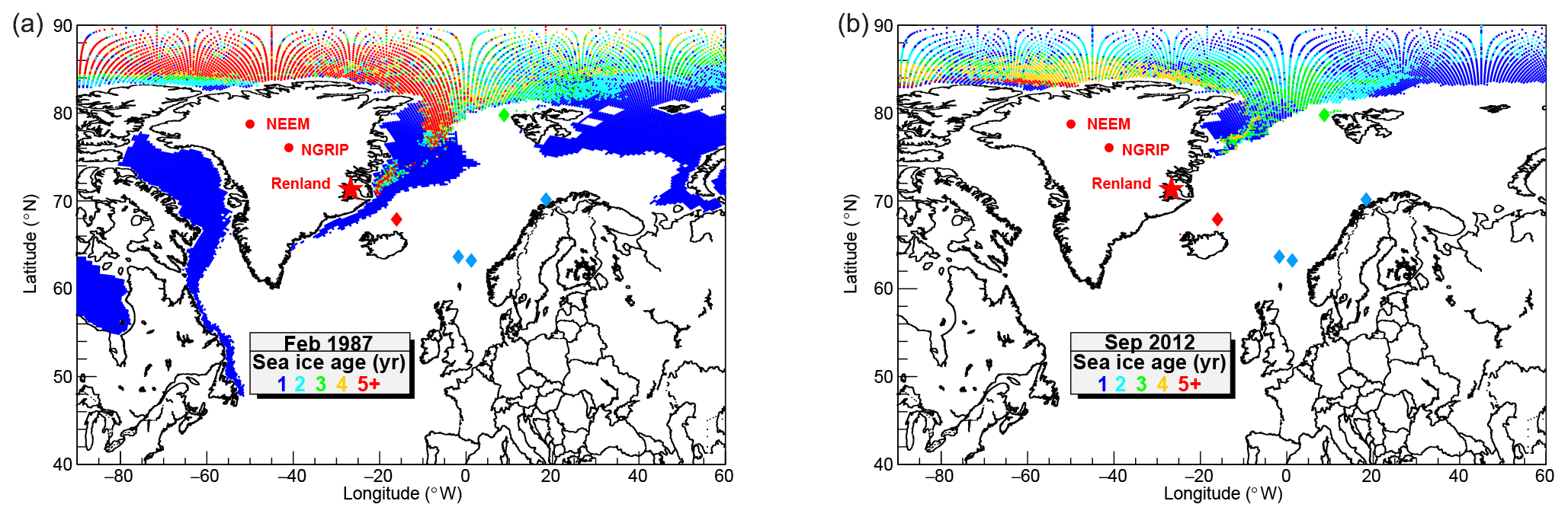
Figure 2 Map of modern Arctic sea ice age shown in representative extreme conditions: winter maximum (February 1987, a) and summer minimum (September 2012, b). The marine cores discussed in the text are indicated by coloured diamonds. See Fig. 1 for the marine core names and references. The sea ice age data are from NSIDC/NASA (v.3) (Tschudi et al., 2016).

2.3 Atmospheric reanalysis: the source region of bromine and sodium for the RECAP ice core

To estimate the source of bromine and sodium deposited at Renland, daily back trajectories were calculated from 2000 CE to 2016 CE with HYSPLIT4 (Stein et al., 2015; Draxler et al., 1999; Draxler and Hess, 1998, 1997), using publicly available NCEP/NCAR Global Reanalysis meteorological data (1948–present), with a 2.5^∘ resolution in both latitude and longitude (Kalnay et al., 1996). The back trajectories were started daily on an hourly basis at 500 m above the Renland elevation (71.305^∘ N, 26.723^∘ W; 2315 m a.s.l.) for the 17-year time span. The trajectory time was set to be 72 h, representing the average atmospheric lifetime of sea-salt aerosol (Lewis and Schwartz, 2004) and likely a lower limit for inorganic gas-phase bromine compounds. To access the potential marine sources of bromine and sodium, only a subset of the all trajectories is considered. Such selection limits the ensemble to only such trajectories that crossed the marine boundary layer (MBL), defined here as the 900 hPa isosurface (corresponding to approximately 1000 m a.s.l.), for at least 10 h. This pressure value was chosen according to Lewis and Schwartz (2004) and references within. One way to display a map of MBL crossings is the residence time analysis, a spatial distribution of trajectory end points (Ashbaugh et al., 1985). This map indicates that 75 % of the signal originates from the North Atlantic Ocean, extending in latitude from 50 to 85^∘ N (up to the Fram Strait) and in longitude from the western coasts of Norway and the UK to east Greenland (Fig. 1), although the ocean regions closer to Renland are expected to be more significant as per the observed chemical signature. A minor contribution is expected from aerosols and gas-phase bromine originating from coastal waters off west Greenland. The consistency of sea ice reconstructions from the RECAP core and the Nordic Sea sediment cores (Sect. 4.2) suggests that the source area could extend to these regions throughout the last 90 kyr. For the overall interpretation of the RECAP record, the source area is therefore assumed to be the 75 % contour region of the residence time analysis end point distribution (Fig. 1). Such a region is nowadays mostly dominated by open-water (OW) conditions, with only minor contributions of FYSI grown in situ and multi-year sea ice (MYSI) transported south of the Arctic Ocean alongside the east Greenland coastline via the Transpolar Drift (Fig. 2).

3 Calculation of bromine enrichment (Br_enr) and Br_enr time series

The bromine enrichment values in the ice samples are calculated from the departure from the seawater abundance, the latter inferred from sodium (hereafter sea-salt sodium, ssNa), Eqs. (1), (2):

$$\begin{array}{}\text{(1)}& {\displaystyle }{\mathrm{Br}}_{\mathrm{enr}}={\displaystyle \frac{\mathrm{Br}/\mathrm{ssNa}}{(\mathrm{Br}/\mathrm{Na}{)}_{\mathrm{m}}}},\text{(2)}& {\displaystyle }\mathrm{Na}=\mathrm{ssNa}+\mathrm{nssNa},\end{array}$$

where Br, ssNa and nssNa are the bromine, sea-salt and non-sea-salt sodium concentrations in the ice samples respectively, and $(\mathrm{Br}/\mathrm{Na}{)}_{\mathrm{m}}=\mathrm{0.0062}$ is the bromine-to-sodium mass ratio in seawater (Millero et al., 2008), assumed to be constant in time and space. Since sodium concentrations in ice cores can be interfered with by terrestrial inputs (nssNa, from sodium oxide Na₂O), which can generally contribute up to ≈10 %–50 % during glacial arid periods (i.e. stadials), nssNa and ssNa have to be evaluated to calculate Br_enr (Eqs. 1–2). We estimate the ssNa concentrations by using three methods. They make use of chlorine, magnesium and calcium concentrations.

The decrease in the Cl∕Na mass ratio from the seawater reference (1.8 from Millero et al., 2008) can be related to extra sodium inputs of terrestrial origin. Thus, the ssNa can be calculated from chlorine if the measured chlorine-to-sodium ratio becomes less than 1.8, while zero nssNa is assumed otherwise (Eqs. 3–4):

$$\begin{array}{}\text{(3)}& {\displaystyle }\mathrm{ssNa}={\displaystyle \frac{\mathrm{Cl}}{\mathrm{1.8}}}⟷{\displaystyle \frac{\mathrm{Cl}}{\mathrm{Na}}}<\mathrm{1.8},\text{(4)}& {\displaystyle }\mathrm{ssNa}=\mathrm{Na}⟷{\displaystyle \frac{\mathrm{Cl}}{\mathrm{Na}}}\ge \mathrm{1.8}.\end{array}$$

Unfortunately, sea-salt aerosols are affected by acid-scavenged (HNO₃ and H₂SO₄) dechlorination processes (e.g. $\mathrm{2}\mathrm{NaCl}+{\mathrm{H}}_{\mathrm{2}}{\mathrm{SO}}_{\mathrm{4}}\to \mathrm{2}\mathrm{HCl}+{\mathrm{Na}}_{\mathrm{2}}{\mathrm{SO}}_{\mathrm{4}}$), in which chlorine is removed as gas-phase HCl. These processes would increase the Cl∕Na ratios in ice beyond the seawater reference (Legrand and Delmas, 1988), especially in warmer climatic conditions, since HCl is believed to have a longer atmospheric residence time than SSA. In fact, RECAP Holocene Cl∕Na ratios (≈3) suggest that dechlorination processes do occur and chlorine is also deposited as HCl. Additionally, this result shows that HCl loss from the snowpack after deposition is limited, opposite to what is observed in Antarctica (Dome C) (Röthlisberger et al., 2003). The huge difference between Dome C and Renland accumulation rates likely explains such a polar asymmetry. In glacial ice, and especially during MIS 2 and MIS 4, the effect of dust neutralization of nitric and sulfuric acids would reduce chlorine loss both after deposition and during transport, therefore making the above correction more trustworthy (Wolff et al., 1995). However, the relative contributions of dechlorination processes and dust loading as per the observed Cl∕Na ratios in the ice are difficult to quantify. A correction based on Cl∕Na ratios was used by Hansson (1994) to calculate the ssNa and nssNa concentrations in the Renland core drilled in 1988. In particular, they found that nssNa accounts for respectively 17 % and 24 % of the total sodium during MIS 2 and MIS 4. If the same correction is applied to our measurements, we find values of 15 % and 20 %–30 % during MIS 2 and MIS 4.

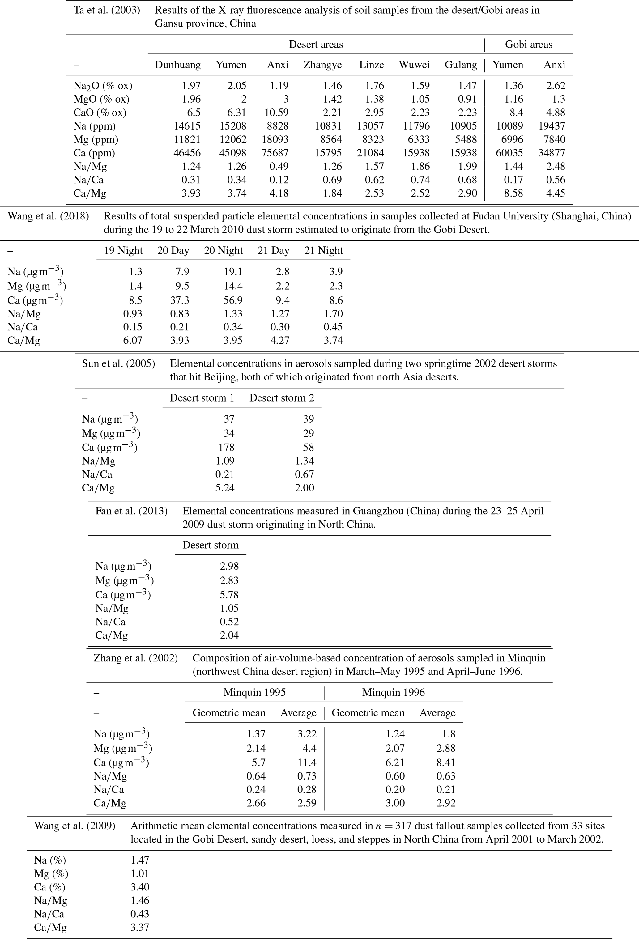
A better alternative to calculate ssNa and nssNa would be to use an element of terrestrial origin. Magnesium contains both a marine and a terrestrial signature. By using reference mass ratios of Na∕Mg in seawater and in the Earth upper continental crust, we are able to calculate the marine sodium contribution (Eq. 7). Often in ice core studies, the sea-salt and non-sea-salt contributions are calculated using global-mean reference values of the chemical composition of terrestrial elements (see for example Rudnick and Gao, 2003, Table 1). However, the spatial variability of the dust mineralogy can heavily impact the results. In our case, the terrestrial value (Na∕Mg)_t to be used in the calculation (the subscript “t” refers to “terrestrial”) would require knowledge of the geochemical composition of the dust deposited at Renland. In remote Greenlandic ice cores, the provenance of aeolian mineral dust is believed to be the deserts in north-east Asia, as inferred from Sr, Nd and Pb isotopic ratios (Biscaye et al., 1997). We therefore carried out a compilation of present-day Na∕Mg mass ratios of dust sourced from north-east Asian deserts, assuming that such an Asian dust source remained the dominant one over the last 120 kyr. For such analysis, the reader is referred to Appendix B, which considers n=6 studies of dust composition (Na, Mg and Ca) from the Gobi and desert regions of Mongolian and from northern China deserts. This analysis (Appendix B) shows that, on average, dust from these regions exhibits the following ratios:

$$\begin{array}{}\text{(5)}& {\displaystyle }{(\mathrm{Na}/\mathrm{Mg})}_{\mathrm{t}}=\mathrm{1.23},\text{(6)}& {\displaystyle }{(\mathrm{Na}/\mathrm{Ca})}_{\mathrm{t}}=\mathrm{0.38}.\end{array}$$

It is worth noting that these values differ substantially from global average values (Rudnick and Gao, 2003), especially for Na∕Ca. By using the sodium-to-magnesium ratios in Asian dust ${(\mathrm{Na}/\mathrm{Mg})}_{\mathrm{t}}=\mathrm{1.23}$ (Eq. 5) and in seawater ${(\mathrm{Mg}/\mathrm{Na})}_{\mathrm{m}}=\mathrm{0.12}$ (Millero et al., 2008) (the subscript “m” refers to “marine”), we are able to calculate ssNa and ssMg (Eqs. 7–8):

$$\begin{array}{}\text{(7)}& {\displaystyle }\mathrm{ssNa}={\displaystyle \frac{\mathrm{Na}-{(\mathrm{Na}/\mathrm{Mg})}_{\mathrm{t}}\cdot \mathrm{Mg}}{\mathrm{1}-{(\mathrm{Mg}/\mathrm{Na})}_{\mathrm{m}}\cdot {(\mathrm{Na}/\mathrm{Mg})}_{\mathrm{t}}}},\text{(8)}& {\displaystyle }\mathrm{ssMg}={\displaystyle \frac{{(\mathrm{Mg}/\mathrm{Na})}_{\mathrm{m}}\cdot \mathrm{Na}-{(\mathrm{Mg}/\mathrm{Na})}_{\mathrm{m}}\cdot {(\mathrm{Na}/\mathrm{Mg})}_{\mathrm{t}}\cdot \mathrm{Mg}}{\mathrm{1}-{(\mathrm{Mg}/\mathrm{Na})}_{\mathrm{m}}\cdot {(\mathrm{Na}/\mathrm{Mg})}_{\mathrm{t}}}}.\end{array}$$

In the Holocene, on average ssNa ≈0.99 Na, while ssMg ≈0.50–0.90 Mg. During MIS 2, ssNa ≈0.6–0.7 Na and ssMg ≈0.20–0.30 Mg, while during MIS 4 ssNa ≈0.50–0.60 Na and ssMg ≈0.10–0.20 Mg. In those Holocene samples where magnesium was not measured, we assume Na = ssNa, making on average a 1 % error.

Figure 3 Calcium and magnesium concentrations in the RECAP core. Samples with high (>100 ppb) calcium concentrations are drawn in blue. The red samples of the bottom 22 m (562–584 m depth) are not dated but may consist of Eemian ice (see main text). All others samples are drawn in green. The Ca∕Mg ratio varies between 3±1 (Asian dust) and 23±1 (gypsum and/or excess of carbonate). The seawater ratio ${(\mathrm{Ca}/\mathrm{Na})}_{\mathrm{m}}=\mathrm{0.32}$ cannot be identified.

The same procedure using calcium instead of magnesium has been applied to calculate ssNa concentrations from Antarctic ice cores (Röthlisberger et al., 2002), by solving the equations similar to Eqs. (7) and (8) with Mg replaced by Ca. In the RECAP record, such a correction using Asian dust ${(\mathrm{Na}/\mathrm{Ca})}_{\mathrm{t}}=\mathrm{0.38}$ and marine ${(\mathrm{Ca}/\mathrm{Na})}_{\mathrm{m}}=\mathrm{0.038}$ (Millero et al., 2008) unrealistically predicts ssNa ≈0 throughout the glacial period. Small changes in the (Na∕Ca)_t value do not significantly change this result. It appears that higher than expected calcium is deposited at Renland, and therefore a lower (Na∕Ca)_t is to be used. The excess of calcium during the glacial period has been reported in Greenlandic ice cores, in the form of calcite (CaCO₃), dolomite (CaMg(CO₃)₂) and gypsum (CaSO₄⋅2H₂O) minerals (Mayewski et al., 1994; Maggi, 1997; De Angelis et al., 1997). In their investigation of the GRIP ice core Legrand and Mayewski (1997) find a larger increase in sulfate (${\mathrm{SO}}_{\mathrm{4}}^{\mathrm{2}-}$) in Greenland compared to Antarctica during glacial times. Such large enhancements of the sulfate level are well correlated with calcium increases but not with MSA, suggesting that sulfate levels are related to non-biogenic sulfur sources (gypsum emissions from deserts, for instance) (Legrand and Mayewski, 1997). Different calcium sources were likely active during the glacial period as compared to warmer periods, but it is unclear whether these were new active continental sources or continental shelves which became exposed due to a lowered sea level. Similarly to what has been observed in other Greenland ice cores, extra calcium is also found in the RECAP core during the glacial, as illustrated from the scatter plot with magnesium (Fig. 3). From this calcium–magnesium relation, we estimate that during the coldest and most arid glacial times $(\mathrm{Ca}/\mathrm{Mg}{)}_{\mathrm{t}}=\mathrm{23}\pm \mathrm{1}$ (blue fit in Fig. 3), while in other periods we assume that the composition remained the same as the modern Asian dust composition (Appendix B):

$$\begin{array}{}\text{(9)}& {\left({\displaystyle \frac{\mathrm{Ca}}{\mathrm{Mg}}}\right)}_{\mathrm{t},\mathrm{modern}}=\mathrm{3.7}.\end{array}$$

This hypothesis is substantiated by the value found for the lower envelope for the Holocene, interstadial late MIS 5 samples (green points in Fig. 3) as well as for composition of the bottom 22 m of the core (562–584 m, red points in Fig. 3): $(\mathrm{Ca}/\mathrm{Mg}{)}_{\mathrm{t}}=\mathrm{3}\pm \mathrm{1}$ (red fit). We note that these bottom measurements do not appear in any time series since the core chronology ends at 120 ka (562 m). We therefore here suggest that the RECAP bottom 22 m date back to the previous interglacial, the Eemian.

Sea-salt sodium concentrations (ssNa) can therefore be calculated using calcium, by replacing Mg→Ca in Eq. (7) and by using ${(\mathrm{Ca}/\mathrm{Na})}_{\mathrm{m}}=\mathrm{0.038}$ and (Na∕Ca)_t calculated by

$$\begin{array}{}\text{(10)}& {\left({\displaystyle \frac{\mathrm{Na}}{\mathrm{Ca}}}\right)}_{\mathrm{t}}={\displaystyle \frac{{(\mathrm{Na}/\mathrm{Mg})}_{\mathrm{t},\mathrm{modern}}}{{(\mathrm{Ca}/\mathrm{Mg})}_{\text{t, glacial fit}}}}={\displaystyle \frac{\mathrm{1.23}}{\mathrm{23}}}=\mathrm{0.054}.\end{array}$$

As a comparison, in the GRIP core, where the ssNa calculations were based on a mixed chlorine–calcium method, De Angelis et al. (1997) found empirically that ${(\mathrm{Na}/\mathrm{Ca})}_{\mathrm{t},\mathrm{glacial}}=\mathrm{0.036}$ in glacial ice (significant correlation, ρ=0.7) and ${(\mathrm{Na}/\mathrm{Ca})}_{\mathrm{t},\mathrm{modern}}=\mathrm{0.07}$ (weak correlation, ρ=0.2) in Holocene ice.

Figure 4 The 120 kyr time series of analyte concentrations in the RECAP ice core. The last 8 kyr are 100-year averages. (a) bromine; (b) total sodium and sea-salt sodium (ssNa) series calculated using chlorine (green), magnesium (blue) and calcium (red); (c) chlorine; (d) calcium (black) and magnesium (blue); (e) NGRIP δ¹⁸O from North Greenland Ice Core Project members (2004); (f) NEEM Br_enr from Spolaor et al. (2016b); (g) RECAP Br_enr series (Br_enr,Cl, green and Br_enr,Mg, black) calculated using chlorine and magnesium respectively.

The calculation of RECAP nssCa reveals that calcium contains almost a purely crustal signature: nssCa ≳0.95Ca throughout the record.

The ssNa curves calculated with magnesium and calcium (ssNa_Mg, ssNa_Ca) differ by less than 1σ, while appreciable differences between these two curves and the chlorine one (ssNa_Cl) are only found during MIS 2 and MIS 4 (Fig. 4b). A weak positive correlation (ρ=0.32, p<10⁴, n=144) is found between Br and ssNa_Mg concentrations in glacial ice (Appendix C, Fig. C1) suggesting that although the two elements share a common marine source, other source or transport effects are playing a role in driving changes in their respective ice concentrations.

Since ssNa_Mg ≃ ssNa_Ca, for the following discussion we will only consider the two Br_enr series based on the chlorine and magnesium calculation: Br_enr,Cl and Br_enr,Mg (Fig. 4g). Standard error propagation is carried out to yield the final Br_enr uncertainties.

This analysis along with past studies demonstrate that the sea-salt and non-sea-salt calculations of elemental concentrations depend on the chemical composition of the dust that is deposited at the ice core site. The dust composition has a spatial variability which should be considered, while the use of tabulated reference values should be discouraged.

From the two calculated RECAP Br_enr curves (Br_enr,Cl, Br_enr,Mg), we now investigate past sea ice conditions in the 50–85^∘ N North Atlantic Ocean, based on the aforementioned hypotheses on the Br_enr use as an indicator of first-year sea ice conditions. Because of the RECAP location, the record is sensitive to ocean processes and sea ice dynamics (Cuevas et al., 2018; Corella et al., 2019). We compare our sea ice record with PIP₂₅ results from five marine sediment cores drilled within the Renland source area: the Fram Strait, the Norwegian Sea and the North Icelandic shelf. The PIP₂₅ index is a semi-quantitative indicator of the local sea ice conditions at the marine core location. It is calculated by coupling the sediment concentration of IP₂₅, a biomarker produced by diatoms living in seasonal sea ice, with an open-water phytoplankton biomarker (brassicasterol or dinosterol, hence P_BIP₂₅ or P_DIP₂₅). Briefly, the PIP₂₅ index is a dimensionless number varying from 0 to 1: PIP₂₅ ≈ 1 indicates perennial sea ice cover; PIP₂₅ ≈0 indicates open-water conditions, while intermediate PIP₂₅ values reflect seasonal sea ice (Müller et al., 2011; Belt and Müller, 2013).

4 Results and discussion

The two Br_enr time series (Br_enr,Cl and Br_enr,Mg), based on either chlorine or magnesium for the sea-salt sodium calculation, display values greater than 1 throughout the record, suggesting an FYSI signature throughout the last 120 kyr in the North Atlantic (Fig. 4g). The very low values found in the Holocene (on average Br_enr,Hol =3.9, rms (root mean square) =1.5) suggest minimum FYSI during the current interglacial. Although the record does not extend to the Eemian period, it shows that at the inception of the last glacial period, ∼120 000 years ago, Br_enr values were higher than in the Holocene (on average Br_{enr,120 kyr} =5.4, rms =1.1, n=38), suggesting that more FYSI was present at that time. From 120 kyr ago the Br_enr levels increased until the Greenland Interstadial 21 (GI-21), ∼85–80 kyr ago (${\mathrm{Br}}_{\mathrm{enr},\mathrm{85}-\mathrm{80}\mathrm{kyr}}$ ≃8). Hereafter, they decreased throughout late MIS 5. From late MIS 5 to MIS 4, rising Br_enr values are observed, but a statistically significant difference between the two Br_enr curves results from the two ssNa corrections, with the Br_enr,Mg series showing higher values than Br_enr,Cl. The two series converge again at the beginning of MIS 3, with values around 7±1. From ∼50–40 ka, both series start to decrease. The decrease is more significant for Br_enr,Cl. Minimum Br_enr values are reached at the Last Glacial Maximum during MIS 2. The deglaciation reveals a Br_enr increase up to ca. 12 000 years ago, followed by a steady decrease towards the Holocene.

The first Arctic glacial–interglacial investigation of Br_enr was performed on the NEEM ice core, located in northwest Greenland. At NEEM, the main source regions for sea-ice-related processes are believed to the Canadian archipelago, the Baffin Bay and the Hudson Bay (Spolaor et al., 2016b; Schüpbach et al., 2018). The 120 000-year NEEM record (Spolaor et al., 2016b) showed higher Br_enr values during the Holocene and interstadials compared to the glacial stadials (Fig. 4f). This was interpreted as greater FYSI conditions existing during such warmer periods, while the lower Br_enr values during colder climate phases would indicate more extended MYSI coverage in those ocean regions. In accordance with their respective source regions, the Br_enr record from the NEEM ice core is markedly different from the RECAP one (Fig. 4). In the NEEM core, Br_enr was positively correlated to δ¹⁸O throughout the entire climatic record. In contrast, at Renland, such a consistent correlation is not present, and Br_enr is at times lower during warmer climate periods (e.g. during the Holocene). We suggest that this difference originates from the fact that during warm periods, the relative FYSI-to-OW influence is greater at NEEM than at Renland, the latter being mostly dominated by OW conditions in the North Atlantic. This is supported, at least for present conditions, by a model study that investigated the Arctic spatial variability of the ratio of sea ice to open-ocean sodium loadings (Rhodes et al., 2018), where it was found that such ratio at NEEM is ∼5 times higher than Renland.

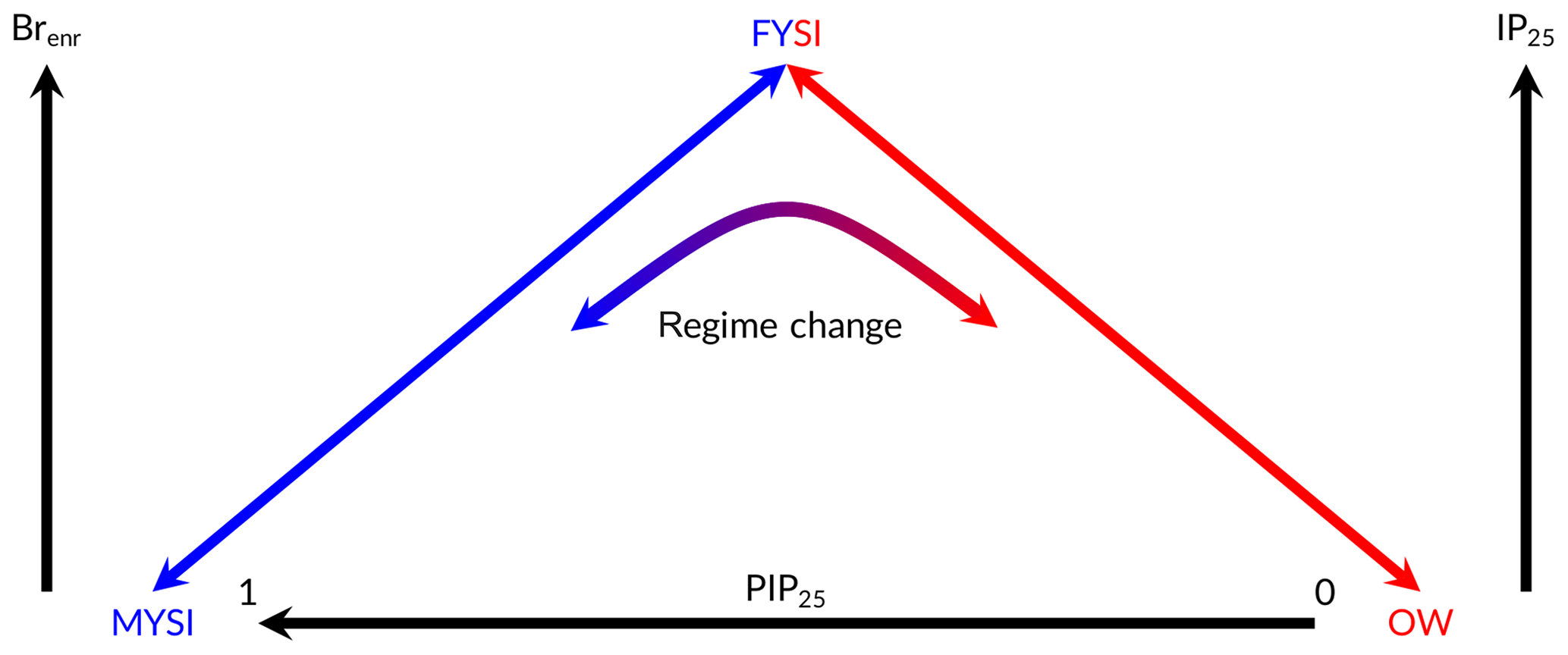
Figure 5 Schematic illustration of marine and (suggested) ice-core-based sea ice indicators as a function of different sea ice conditions. Br_enr (ice core) and IP₂₅ (sediment core) increase as a function of first-year sea ice (FYSI) area. Low values can thus indicate either open-water (OW) or multi-year sea ice (MYSI) conditions, depending on the climate state. The PIP₂₅ index is a marine-derived semi-quantitative indicator of local sea ice conditions at the marine core location. PIP₂₅ ∼0 (PIP₂₅ ∼1) indicates open-water (perennial sea ice, i.e. MYSI) conditions, while intermediate PIP₂₅ values reflect seasonal sea ice (i.e. FYSI). Br_enr values in the RECAP core are believed to indicate an FYSI/OW regime in a “warm” climate state and an FYSI/MYSI in a “cold” climate state.

Since the increase in atmospheric bromine is believed to reflect the strength of bromine recycling from FYSI surfaces, low values of Br_enr could indicate either OW or MYSI conditions. Thus, we suggest that Br_enr is a signature, at Renland, of contrasting sea ice states: FYSI/MYSI and FYSI/OW. We also suggest that the former (FYSI/MYSI) occurs during generally colder periods while the latter (FYSI/OW) occurs during generally warmer periods. In the framework of this dual regime behaviour, if the ice core time resolution is high enough, an increase in Br_enr values followed by a maximum and a negative trend should be a signature of an ocean facing gradual changes from open ocean to multi-year sea ice conditions, or vice versa, in the case of monotonically warming or cooling ocean temperatures (Fig. 5). One such regime shift is observed in the RECAP Br_enr record during the deglaciation (Fig. 4g). At the Last Glacial Maximum (LGM, ∼23 ka), the low enrichment values (${\mathrm{Br}}_{\mathrm{enr},\mathrm{Mg},\mathrm{LGM}}$ $=\mathrm{3.3}\pm \mathrm{0.3}$; ${\mathrm{Br}}_{\mathrm{enr},\mathrm{Cl},\mathrm{LGM}}$ $=\mathrm{3.2}\pm \mathrm{0}.$2) suggest reduced FYSI recycling and therefore extensive MYSI conditions (blue arrow in Fig. 5; OW conditions are considered unlikely). Transitioning from the Last Glacial Maximum into the Holocene, Br_enr increases until ∼12 ka (${\mathrm{Br}}_{\mathrm{enr},\mathrm{Mg},\mathrm{12}\mathrm{kyr}}$ $=\mathrm{8.7}\pm \mathrm{0.9}$; ${\mathrm{Br}}_{\mathrm{enr},\mathrm{Cl},\mathrm{12}\mathrm{kyr}}$ $=\mathrm{7.5}\pm \mathrm{0.5}$), indicating maximum FYSI at this time (Figs. 4 and 6). Hereafter, a decrease is observed, as Br_enr continues to drop during the Early Holocene and the proxy operates in the FYSI/OW regime (red arrow in Fig. 5).

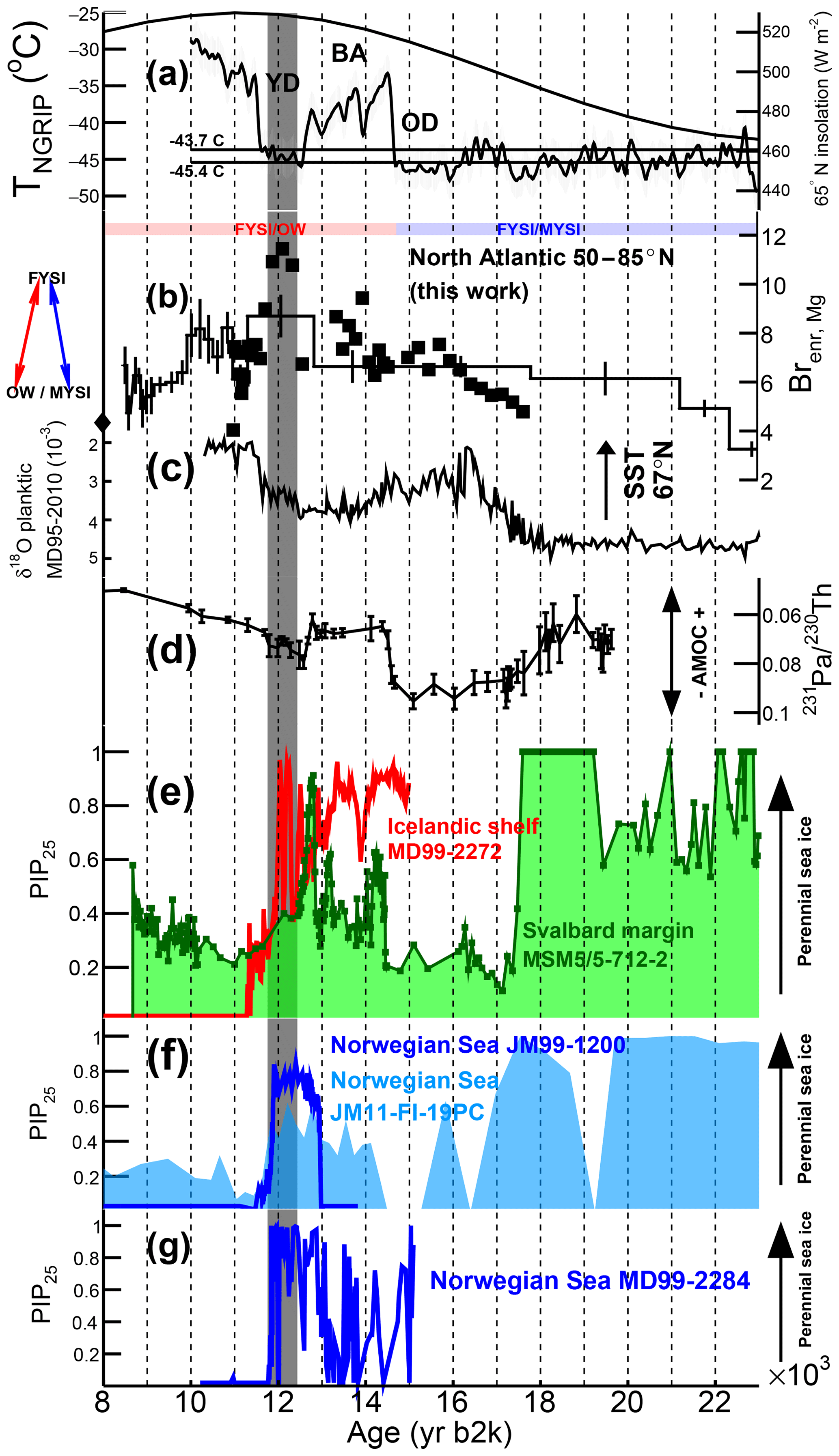
Figure 6 Climate records during the last deglaciation. (a) NGRIP air temperature reconstruction (Kindler et al., 2014) ($\pm \mathrm{1}\mathit{\sigma }=\mathrm{2.5}$ ^∘C). The two horizontal lines correspond to a ±2σ deviation from the mean temperature (−44.6 ^∘C) found during the 12.4–11.8 ka period of maximum Br_enr,Mg (grey vertical band). The T_NGRIP record does not extend before 10 ka but the temperature is not expected to cross the threshold at any time in the Holocene. The black line is the 21 June daily mean insolation at 65^∘ N (Laskar et al., 2004). (b) RECAP Br_enr,Mg (thick black line) and repeat sampling conducted at higher resolution (squares). Since for the highly resolved measurements magnesium was not measured, for the calculation of the sea-salt sodium concentrations and the Br_enr,Mg values (Eqs. 1–7) we used the magnesium values of the four low-resolution samples. Over the time period covered by the repeat measurements, nssNa ≃10 %–20 %. The average Br_enr,Mg value measured during the Holocene is indicated by a diamond. (c) Planktonic δ¹⁸O record from sediment core MD95-2010 (66^∘41.05^′ N, 04^∘33.97^′ E, from Dokken and Jansen, 1999). Lower δ¹⁸O values indicate warmer and fresher ocean waters. (d) Record of ²³¹Pa∕²³⁰Th ratios within a sediment core retrieved in the deep western subtropical Atlantic (33^∘42^′ N, 57^∘35^′ W). Sedimentary ²³¹Pa∕²³⁰Th are believed to reflect Atlantic meridional overturning circulation (AMOC) strength (McManus et al., 2004). (e, f, g) PIP₂₅ records from the Svalbard margin (green, core MSM5/5-712-2, Müller and Stein, 2014), the North Icelandic shelf (red, core MD99-2272, Xiao et al., 2017) and the Norwegian Sea (core JM11-FI-19PC from Hoff et al., 2016); core JM99-1200 from Cabedo-Sanz et al. (2013); and core MD99-2284 from Muschitiello et al. (2019). The PIP₂₅ scale varies from perennial sea ice (PIP₂₅ ≈1) to open-water (PIP₂₅ ≈0) conditions (see Fig. 5). See Fig. 1 for the PIP₂₅ core locations.

4.1 The last deglaciation and the dual Br_enr regimes

We now consider in further detail the last deglaciation, when a number of ocean temperature, salinity, circulation and sea ice changes are observed in the Nordic Seas (Fig. 6). Marine-derived local sea ice records from both the Svalbard margin and the Norwegian Sea indicate (Fig. 6e, f) that near-perennial sea ice (PIP₂₅ ≈0.5–1) was present during MIS 2 until ∼17 ka (17.6 ka recorded in the Svalbard margin), the onset of a major break-up of extensive sea ice cover, during Heinrich Event 1 (18 to 15 ka). Synchronous to within a few centuries, several modifications relevant to the North Atlantic Ocean are observed (Fig. 6), including seawater surface freshening and warming in the polar and subpolar North Atlantic (the 67^∘ N Dokken and Jansen, 1999, record is shown as an example in Fig. 6c) and a near total cessation of the Atlantic Meridional Overturning Circulation (AMOC; Fig. 6d). Generally low to intermediate PIP₂₅ values (PIP₂₅ ≈0–0.5) are reported in the Svalbard Margin and in the Norwegian Sea in the ∼17–12 ka period (Fig. 6e, f, g), with a slight increasing trend throughout the Bølling–Allerød (BA) and a broad maximum reached during the Younger Dryas (YD), suggesting that seasonal sea ice conditions were dominating this period. Other studies from marine records in the Nordic Seas records also suggest milder sea ice conditions during the BA and increased sea ice during the YD (Belt et al., 2015; Cabedo-Sanz et al., 2016). In contrast, a record from the North Icelandic shelf (Fig. 6e) shows that here the sea ice conditions remained near-perennial from 14.7 to 11.7 ka (PIP₂₅ ≈0.5–1). The authors (Xiao et al., 2017) suggest that this pattern of more severe sea ice conditions in the north of Iceland is, at least during the BA and the YD, linked to the flow of warmer waters from the North Atlantic Current, influencing sea ice melting in the eastern Nordic Seas, whereas the Icelandic shelf is influenced by colder polar waters from the East Greenland Current and the East Icelandic Current.

The RECAP ice core was resampled at a sub-centennial resolution to better constrain the timing of sea ice changes through the deglaciation in the 50–85^∘ N North Atlantic (Fig. 6b, squares). The Br_enr,Mg series (Br_enr,Cl would lead to the same results) would indicate that FYSI started to increase in the North Atlantic, concurrent with a reduction in MYSI, at ∼17.5 ka, synchronous with a local PIP₂₅ decrease in the Svalbard margin and eastern Nordic Seas and in response to sea surface temperature warming in the North Atlantic. This finding would also suggest that North Atlantic sea ice changes occurred in concert with temperature and circulation changes in the underlying surface waters. We note that this time period also coincides with the initiation of deglacial changes in mean ocean temperature, Antarctic temperatures and atmospheric CO₂ concentrations toward interglacial values (Bereiter et al., 2018). North Atlantic FYSI continued to increase throughout the BA (except for one point at 12.7–12.4 ka at the onset of the YD) until a maximum at 12.4–11.8 ka during the YD, when a clear Br_enr,Mg maximum is observed (Fig. 6b). From the comparison between the marine and ice core results, we infer that, during the 17–12 ka period, the 50–85^∘ N-integrated North Atlantic sea ice changed from MYSI to FYSI. Local sea ice was also melting at ∼17 ka in the eastern Nordic Seas, likely influenced by the North Atlantic Current, while, at least from 14.7 to 11.7 ka, sea ice was still near-perennial at the North Icelandic shelf, possibly due to the influence of cold waters carried by the East Greenland Current. Following its maximum value at 12.4–11.8 ka, Br_enr (i.e. FYSI) started to decrease (Fig. 6b). We suggest that from this point in time, the Br_enr indicator now shifts to the FYSI/OW regime (Fig. 5), and the North Atlantic basin becomes largely ice free. A retreating FYSI scenario is also recorded in all five marine cores (decreasing PIP₂₅ to ≈0–0.4 during the Early Holocene; Fig. 6e, f, g), suggesting that open-water conditions progressively developed in the whole North Atlantic basin, sustained by increasing heat transport from the North Atlantic Current and a strengthened AMOC since ∼11.7 ka (McManus et al., 2004; Ritz et al., 2013).

Since Br_enr is assumed to be an increasing function of FYSI, its decrease would point to either OW or MYSI conditions, following either the FYSI/OW or the FYSI/MYSI regimes (Fig. 5). At any point in time, only one regime is considered to be in place, and we suggest a simple model in which a temperature threshold could be the discriminating variable setting the regime type. Since a change in regime is observed during the deglaciation, with maximum Br_enr values (i.e. FYSI) at 11.8–12.4 ka, we set the threshold to be the mean NGRIP ice core temperature reconstructed for that period: ${\mathrm{T}}_{\mathrm{NGRIP}}=-\mathrm{44.6}\pm \mathrm{0.9}$ (2σ) ^∘C (the two lines in Fig. 6a). In every ice sample of the 120 000-year record the regime type (FYSI/MYSI or FYSI/OW; Fig. 5) can thus be determined according to its integrated temperature value with respect to the temperature threshold: FYSI/MYSI for a lower temperature value and FYSI/OW for a higher temperature value.

According to this simple model the deglaciation is characterized by the FYSI/MYSI regime until the onset of the Bølling–Allerød (except few points at which the regime type depends on the chosen threshold value; Sect. 4.2), while the FYSI/OW regime operated from that point forward. We note that there is no similar Br_enr maximum at the onset of the Bølling–Allerød as seen in the YD at the point when NGRIP temperature is crossing the same temperature as found in the YD. The possible explanation of higher Br_enr values during the Younger Dryas compared to the Bølling–Allerød may reside in the higher seasonal temperature variations (Buizert et al., 2014) and freshwater inputs from melting ice sheets in the former period, both promoting the formation of seasonal sea ice. Conversely, the lower Br_enr values (hence to greater MYSI in the FYSI/MYSI regime) during the Older Dryas compared to the Bølling–Allerød and the Younger Dryas may be linked to the overall much lower temperatures during this period (Buizert et al., 2014), higher surface water salinity due to less freshwater inputs from melting ice sheets and a generally weaker AMOC. It appears that the NGRIP temperature threshold alone is unable to fully represent the suggested two-regime modelization during the deglaciation, possibly due to concomitant changes in other sea-ice-related climate variables during this period. We suggest that at glacial–interglacial timescales such a temperature-based discrimination could be still used to represent the two-regime variability.

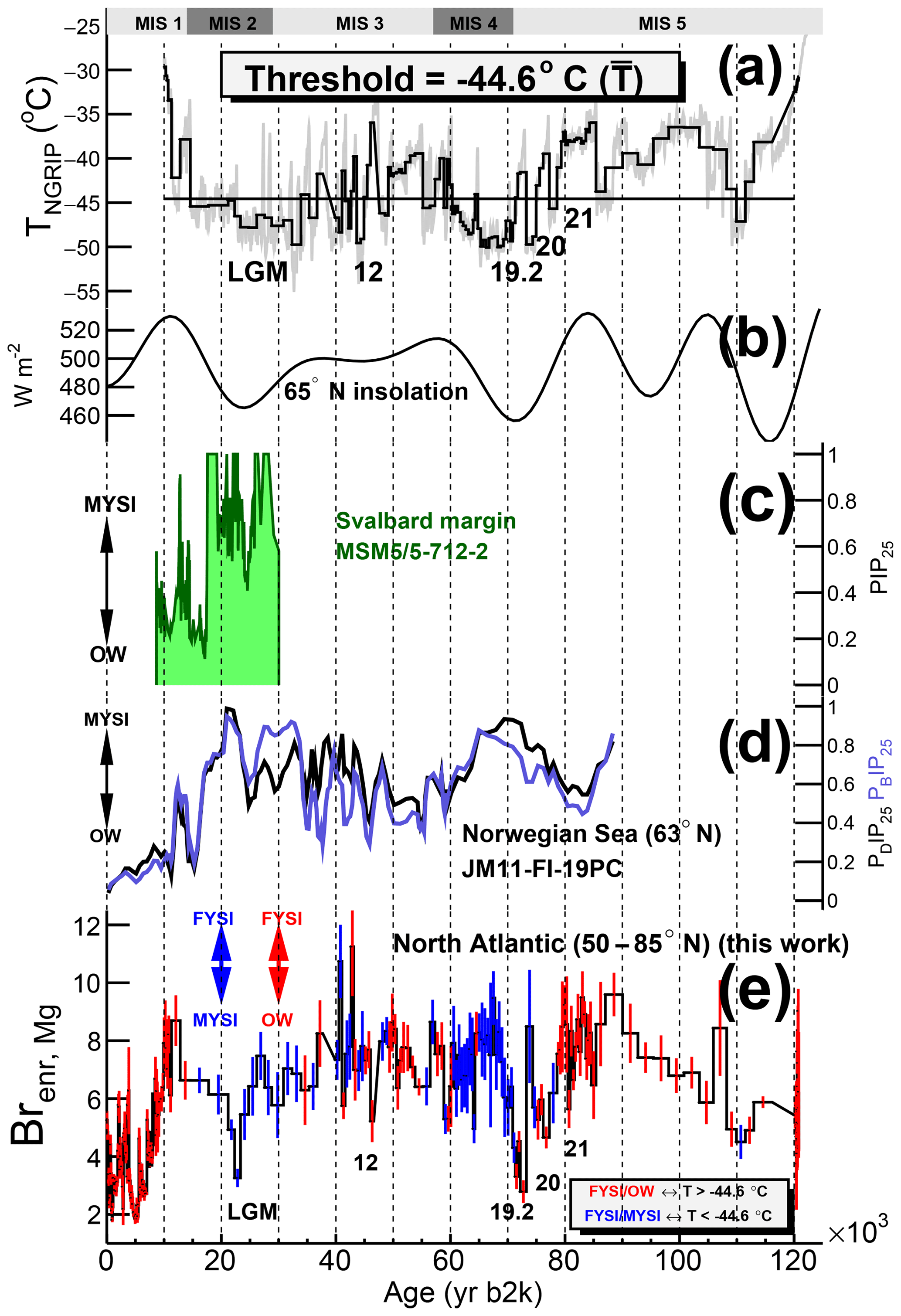
Figure 7 Discrimination between the two Br_enr,Mg regimes according to the −44.6 ^∘C NGRIP temperature threshold and North Atlantic sea ice records from marine cores. (a) Reconstructed NGRIP temperature (grey; Kindler et al., 2014). The temperature threshold value is the mean temperature during the 11.8–12.4 ka period, when the change in Br_enr,Mg regime was observed (see Fig. 6). The black series is the NGRIP temperature profile downscaled to the measured Br_enr resolution. The numbers indicate the Greenland Interstadials (GIs) discussed in the text. (b) Daily mean insolation on 21 June at 65^∘ N (Laskar et al., 2004). (c) PIP₂₅ record from the Svalbard margin (core MSM5/5-712-2 from Müller and Stein, 2014). (d) P_DIP₂₅ and P_BIP₂₅ 90 kyr records from the Norwegian Sea presented as five-point running mean (from Hoff et al., 2016). (e) Discrimination between the Br_enr,Mg regimes computed according to the integrated temperature value with respect to the threshold. The FYSI/OW and FYSI/MYSI regimes are indicated with red and blue error bars respectively.

4.2 The 120 000-year Br_enr record

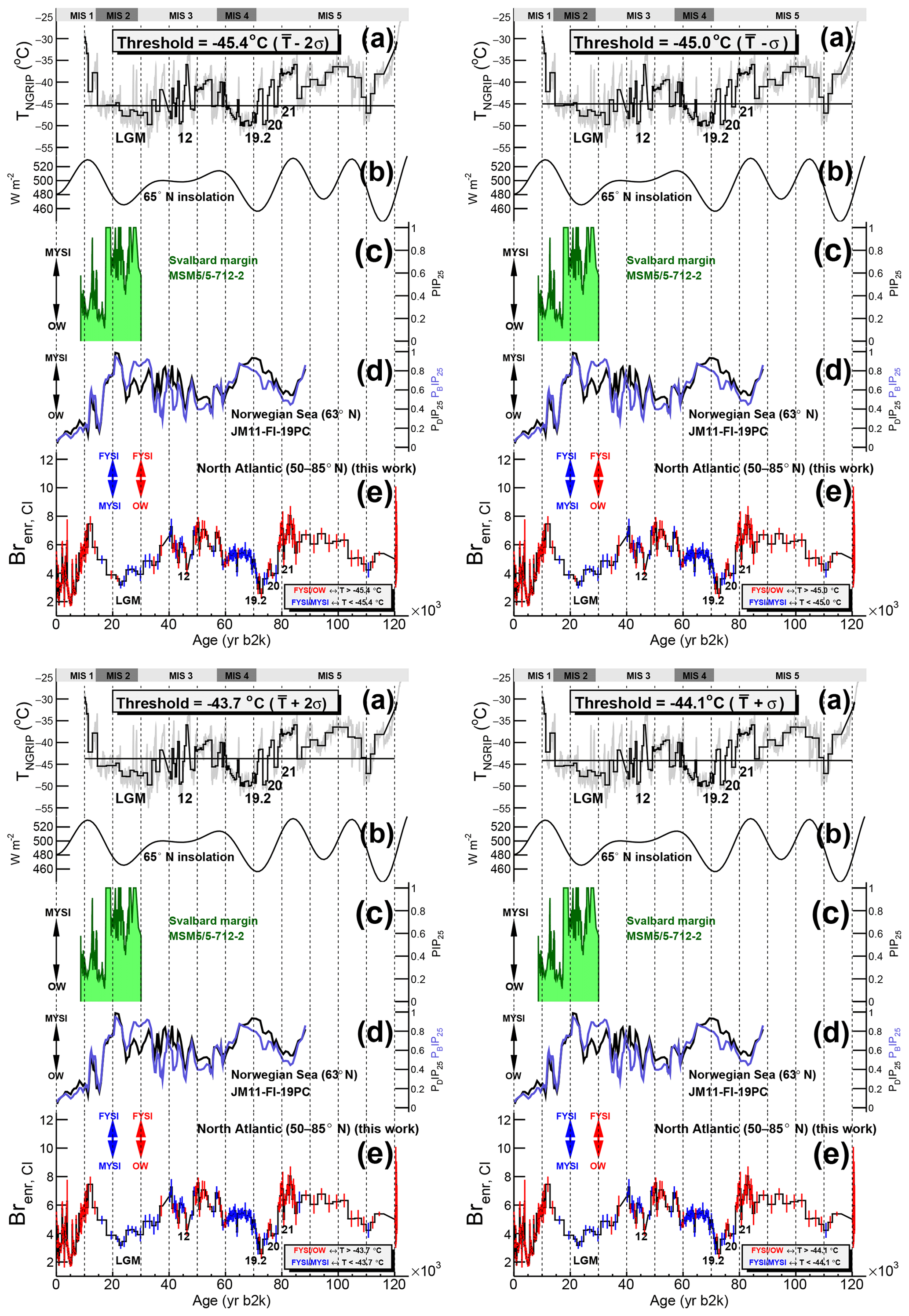
We now apply the previously mentioned temperature-based discrimination between the two sea ice regimes to the 120 000-year Br_enr,Mg record (Fig. 7). The regime type in each ice sample is represented by the colour of the error bars: blue for the FYSI/MYSI regime and red for the FYSI/OW regime. In order to test the sensitivity of the regime output to the threshold value, four scenarios are computed, using a ±1σ and a ±2σ value around the temperature threshold mean value $\stackrel{\mathrm{‾}}{T}=-\mathrm{44.6}$ ^∘C (Fig. D1). Except for 2(1) samples at ca. 20 ka showing a different regime type in the $\stackrel{\mathrm{‾}}{T}$-2(1)σ scenario during the deglaciation (Fig. D1), the regime discrimination mentioned in the following discussion is invariant with respect to the four temperature-based scenarios. The same analysis is also performed on the Br_enr,Cl curves (Fig. D2).

MIS 5 is characterized by increasing Br_enr,Mg values in the FYSI/OW regime from 120 to 80 kyr ago (Greenland Interstadial, GI-21, Fig. 7). We interpret this trend with increasing FYSI extent in the North Atlantic. From the end of GI-21 the Br_enr regime changes to FYSI/MYSI as the NGRIP temperature drops during late MIS 5 and MIS 4. As compared to the levels reached during GI-21 (8±1), lower Br_enr,Mg values are found during GS-21, GS-20 and GS-19 (5±2) and on average during MIS 4 (7±1). We interpret the combined effect of decreased Br_enr,Mg values in the FYSI/MYSI regime with an increase in MYSI extent in the North Atlantic from late MIS 5 to MIS 4. The Br_enr,Cl curve shows even lower values during MIS 4, predicting more extended MYSI than the Br_enr,Mg record (Fig. D2). Overall, from 120 kyr ago to MIS 4, the change in Br_enr regime (from FYSI/OW to FYSI/MYSI) is opposite to what is observed during the deglaciation (from FYSI/MYSI to FYSI/OW): from a relatively warm climate 120 kyr ago, the cooling trend is characterized by an increasing FYSI extent until the point (GI-21) at which the FYSI starts to be replaced by MYSI. This maximum Br_enr,Mg value at the time of the regime change (GI-21) is similar to the peak Br_enr,Mg value reached during the deglaciation: Br_enr,Mg(12 kyr) ≃ Br_enr,Mg(GI-21) ≃8. The same result holds if one considers the Br_enr,Cl series (Fig. D2). Unlike the longer lasting GI-21, the Greenland Interstadials GI-20 and GI-19.2 display very low Br_enr values (≃3–5). A possible explanation for these low values could be found in a fast replacement (at least not captured by the time resolution of the Br_enr record) of MYSI by OW conditions. Higher time-resolved measurements would be needed to test this hypothesis.

Moving from MIS 4 to MIS 3, the Br_enr,Mg values remain within 1σ of each other. This suggests a similar FYSI extent in the two periods, although the FYSI/MYSI regime operating during MIS 4 could suggest an extra MYSI extent during this period, as compared to MIS 3, the latter being generally characterized by a mixture of both Br_enr regimes. This hypothesis is supported by the Br_enr,Cl series, which shows lower values during MIS 4 than MIS 3 (Fig. D2). A sea ice record in the Norwegian Sea (Hoff et al., 2016) also indicates more perennial sea ice conditions during MIS 4 than during MIS 3. The time resolution does not allow a deep investigation of DO events during MIS 3, although a low Br_enr value in the FYSI/OW regime during the GI-12 (Br_enr,Mg(46.0–46.6 ka) $=\mathrm{5.2}\pm \mathrm{0.7}$) suggests a shift to open-water conditions during this interstadial, similarly to GI-19.2 and GI-20. Possibly, similar sea ice dynamics were in play during these stadial–interstadial transitions. Increased time resolution is, however, needed to better characterize DO events.

MIS 2 is characterized by an FYSI/MYSI regime and progressively decreasing Br_enr,Mg values (Fig. 7e), with a minimum being reached ∼23 kyr ago, during the Last Glacial Maximum: Br_enr,Mg(LGM) $=\mathrm{3.3}\pm \mathrm{0.3}$. We interpret this negative Br_enr,Mg (and Br_enr,Cl, Fig. D2) trend with progressively increasing MYSI conditions in the whole North Atlantic, which reached a maximum during the LGM. Relatively high and increasing PIP₂₅ values (≈0.5–1) are found in the Norwegian Sea record (Fig. 7d), with maximum sea ice registered ca. 20–23 kyr ago. The sea ice record from Fram Strait is in broad agreement with the Norwegian record, the former showing high (≈0.5–1) and variable PIP₂₅ values until the longer lasting 19 ka maximum (Fig. 7c). Overall, the cold MIS 2 period is characterized by decreasing seasonal sea ice and increasing multi-year sea ice across the North Atlantic, with a maximum reached ca. 20 kyr ago.

The deglaciation is characterized by increasing FYSI conditions until the mid-Younger Dryas (12.4–11.8 kyr ago), followed by a return to the FYSI/OW regime and decreasing Br_enr values as open waters progressively replaced sea ice in the Holocene. A clear sea ice decline is also reported in the Norwegian Sea following the LGM towards the current interglacial (Figs. 6 and 7).

5 Conclusions and outlook

We present a 120 000-year record of bromine enrichment (Br_enr) from the RECAP ice core and interpret it in terms of FYSI variability in the 50–85^∘ N-integrated North Atlantic Ocean. The record suggests that, during the last deglaciation, sea ice started to transform from multi-year to first-year ∼17.5 kyr ago, probably triggered by increasing surface ocean water temperatures. Increasing first-year sea ice conditions are observed throughout the Older Dryas, the Bølling–Allerød and the Younger Dryas. During these periods, the availability of freshwater from melting ice sheets, seasonal temperature variations and AMOC strength likely played a role in driving the sea ice changes. The maximum first-year sea ice signature is found 12.4–11.8 kyr ago, during the Younger Dryas, whereupon open ocean was the dominant condition during the Holocene (MIS 1). Although the RECAP sea ice record does not extend back to the warmest period of MIS 5, it does show that sea ice extent during the Holocene is lower than at any time in the past 120 000 years. Minimum first-year sea ice, likely associated with maximum multi-year sea ice conditions existed during MIS 2 and possibly during MIS 4. Compared to MIS 2, greater first-year sea ice extent existed during MIS 3 and MIS 5. Increased time resolution is needed to fully resolve Dansgaard–Oeschger oscillations. However, the data indicate that during GI-12, GI-19.2 and GI-20, large extent of first-year sea ice could have been replaced by open ocean, while large first-year sea ice areas existed during GI-21.

These analyses and conclusions rely on a number of hypotheses and assumptions mainly concerning the validity of Br_enr as a proxy for first-year sea ice. Efforts are still needed in the direction of validating these assumption and investigating the limitations and processes that affect the Br_enr signature in present deposition and in old ice core records.

Appendix A: Bromine loss from the snowpack

The stability of bromine after deposition has been questioned since the first investigation carried out by Dibb et al. (2010) in Summit (Greenland). We summarize here the experimental investigations that have been carried out on this topic ever since both in Antarctica and in the Arctic.

A1 Antarctica

McConnell et al. (2017) investigated simultaneous sodium and bromine fluxes across Antarctica (see their Fig. S4 in the Appendix showing the reconstructed fluxes from an array of 11 cores measured in McConnell et al., 2014). In particular, the J(Na) and J(Br)–accumulation rate (A) linear relations (impressive J(Br)–A linear fit from 50 to 400 kg m⁻² yr⁻¹) suggest that, while sodium loss is negligible, bromine re-emission is quantified to 17±2 µg m⁻² yr⁻¹ (negative intercept, i.e. snow–air flux). According to the results, the bromine loss from Antarctic snowpack would be 65 % at sites with A=50 kg m⁻² yr⁻¹, 32 % at sites with A=100 kg m⁻² yr⁻¹, 22 % at sites with A=150 kg m⁻² yr⁻¹, 16 % at sites with A=200 kg m⁻² yr⁻¹, 13 % at sites with A=250 kg m⁻² yr⁻¹ and 11 % at sites with A=300 kg m⁻² yr⁻¹ (note that this exercise works on the hypothesis that the bromine air concentration is the same above all sites, but the goodness of their fit would suggest that this is the case). These negative fluxes would be representative of Antarctic conditions for the duration of the records, i.e. few centuries to 2 millennia maximum (see Supplement Table S2 in the 2014 ref). In their Dome C (A=30 kg m⁻² yr⁻¹) study, Legrand et al. (2016) analysed bromine content in a 110 cm deep, 2 cm resolution snow pit. Their measurements show that the upper 2 cm contain 1.25 times more bromine that the 2–4 cm layer, 2.5 times more than the 4–8 cm layer and ca. 10 times more than the 8–12 cm layer. Based on the higher bromine concentrations towards the surface the authors suggest a possible bromine remobilization from the snow. In testing the hypothesis, the authors model whether the measured bromine snow content is high enough to sustain the 1.7 pptv air concentration of Br_y they measured in the overlying atmosphere. They find that to explain such a value, the snow bromine storage should be 35 times larger than the actual measurements. They therefore conclude that in Dome C their investigation do not support the importance of snowpack bromine emissions. This conclusion contrasts with what would be concluded by McConnell and co-workers.

From a surface snow experiments carried out in Dome C in 2014 (Antarctica, A=30 kg m⁻² yr⁻¹) by Spolaor et al. (2018), the authors observe constant bromine concentrations from mid-December to mid-January (austral summer). In a similar experiment carried out the following year, from late November to late December 2015, higher bromine concentrations were found in November (late spring) with a decreasing trend towards the end of the year. The authors relate such a drop to a change in the source of the air masses, from coastal to inland, as inferred from back trajectory modelling, rather than to bromine loss from the snow.

Ta et al. (2003)Wang et al. (2018)Sun et al. (2005)Fan et al. (2013)Zhang et al. (2002)Wang et al. (2009)

Table A1 Compilation Na∕Mg, Na∕Ca and Ca∕Mg mass ratios in dust samples originating from north Asia deserts.

From another surface snow experiment carried out at GV7 (Antarctica, A=270 kg m⁻² yr⁻¹), Vallelonga et al. (QSR, 2019) compare bromine fresh surface snow concentrations with snow pit values and suggest, on the basis of similar values between the values in the surface samples and in the surface of the snow pit (that would integrate the values of the surface samples), that at this site bromine is stable after deposition (the McConnell calculation would predict a loss of 12 %). Looking at the 100–300 µg m⁻² yr⁻¹ annual bromine (2010, 2011, 2012, 2013) fluxes calculated along the Talos Dome–GV7 traverse (Maffezzoli et al., 2017), a negative flux of 17±2 µg m⁻² yr⁻¹ would imply that, if present, the bromine loss can be quantified in this region as 6 %–17 %. As McConnell and co-workers point out, it is surprising that the snow–air bromine flux they found is not dependent on snow accumulation (their fit appears linear until the last point: 400 kg m⁻² yr⁻¹).

A2 Arctic

In the Arctic, the most robust piece of evidence results from hourly resolved surface snow measurements carried out in coastal Svalbard, showing that bromine photolytic loss cannot be appreciated across night–day cycles (Spolaor et al., 2019; see Fig. 6).

In an experiment described in QSR (2019) that Vallelonga and co-workers carried out in Ny-Ålesund (Svalbard, A=600 kg m⁻² yr⁻¹), sodium and bromine were measured in surface snow daily from April to June (spring to summer). From April to late May Br_enr values decreased by a factor of 2 (max) (afterwards surface melting and positive temperatures led to 80 % sodium drainage from the snowpack). It is difficult, however, to determine whether this decrease is due to bromine re-emission or to early spring bromine explosions from sea ice surfaces, located ca. 150 km away from the sampling site, enriching the spring deposited snow layers.

A3 Conclusive remarks on bromine loss

To conclude, field experiments aimed at quantifying bromine loss from the snowpack are made difficult by the concurrent effect of other variables (source effects, changes in transport pathways, other postdepositional processes) that can act simultaneously. Estimates of bromine loss from Dome C (Antarctica) have not led to unique conclusions. This site is likely one of the most challenging to carry out this type of study since the snow accumulation is so limited that it is challenging to decipher whether any loss can be attributed to re-emission or wind erosion processes, exposing older layers, which generally have different bromine concentrations. In other parts of Antarctica, McConnell et al. (2017) suggest a bromine snow–air flux of loss of 17±2 µg m⁻² yr⁻¹ regardless of snow accumulation, while at GV7 bromine loss was not detected (Vallelonga et al., QSR, 2019). In the Arctic, photolytic loss was not detected in Svalbard. Other experiments have been shown to be inconclusive due to the presence of surface melting. At sites like Renland (where Holocene melting occurs; see Taranczewski et al., 2019), the extremely high snow accumulation could in general suggest a reduced bromine loss, but again, the 5-fold decrease in snow accumulation during the glacial (preliminary $A_{\mathrm{glacial},\mathrm{stadials}}=\mathrm{100}$ kg m⁻² yr⁻¹ (Bo M. Vinther, unpublished data)) may introduce a possible bromine loss during periods of reduced accumulation, thus increasing Br_enr values during the coldest parts of the record. To test these hypotheses and especially the bromine loss during the glacial, a surface study should be carried out at a 100 kg m⁻² yr⁻¹ accumulation site in Greenland. To conclude, at present there are not enough data available to quantify the possible bromine loss from the Renland ice cap, but if present, and depending on accumulation, the effect would be to increase the measured Br_enr values during the coldest sections of the glacial period.

Appendix B: Modern Na∕Mg and Na∕Ca ratios in dust from northern Asian deserts

The aim of this section is to obtain a reference value for the present-day mass ratios of Na∕Mg and Na∕Ca in Asian dust, since the Gobi and desert regions of Mongolian and northern China (hereafter referred to as Asian dust) are believed to be the main source regions of dust found in Greenlandic ice cores during the glacial period, as inferred from Sr, Nd and Pb isotope composition (Biscaye et al., 1997).

We consider n=6 published studies in which the chemical composition of dust sampled during “desert events” (DSs) was analysed in China. Often these studies are carried out in the framework of pollution-related research. We also include composition data from dust sampled in situ in desert areas. For details on the single studies, we refer the reader to the references in Table A1. We note that our compilation only considers dust samples originating (or sampled directly) from deserts. Other geochemical data from such references that considered trajectories that travelled over other areas (marine or others), are not considered.

By considering all the above-mentioned studies, the mean Na∕Mg mass ratio is 1.23 (median =1.26). The mean Na∕Ca mass ratio is 0.38 (median =0.33). The mean Ca∕Mg mass ratio is 3.66 (median =3.55).

Appendix C: Bromine–sodium correlation in the RECAP ice core

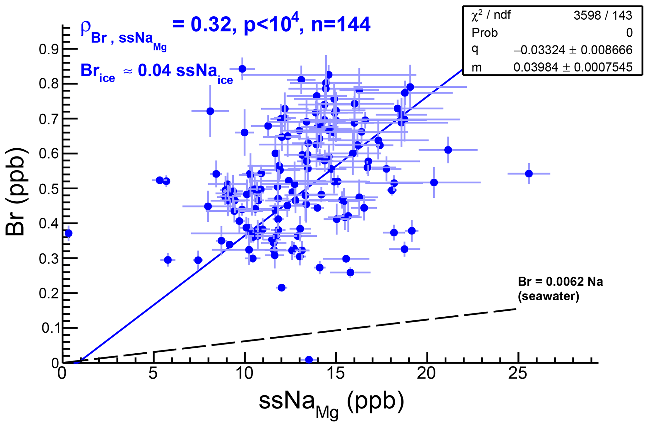
Figure C1 Correlation between bromine and ssNa_Mg concentrations in the glacial section of the RECAP ice core. The weak positive correlation suggests a common source for the two elements. The slope of the (qualitative, p(χ²) ∼0) linear fit indicates significant (∼6) enrichment compared to seawater mass ratios (black line).

Appendix D: Sensitivity of the Br_enr,Mg and Br_enr,Cl regimes to the NGRIP temperature threshold

Figure D1 Sensitivity test of the NGRIP temperature threshold used to perform the Br_enr,Mg regime discrimination (see Fig. D2 for the equivalent analysis using Br_enr,Cl). (a) Reconstructed NGRIP temperature (grey, Kindler et al., 2014). The temperature threshold value is the mean temperature ($\stackrel{\mathrm{‾}}{T}\pm \mathrm{2}\mathit{\sigma }$: left; T±1σ: right) during the 11.8–12.4 ka period, when the change in Br_enr,Mg regime was observed (see Fig. 6). The black time series is the temperature profile downscaled to the measured Br_enr resolution. The numbers indicate the Greenland Interstadials (GIs) discussed in the text; (b) 21 June daily mean insolation at 65^∘ N (Laskar et al., 2004); (c) PIP₂₅ record from the Svalbard margin (core MSM5/5-712-2 from Müller and Stein, 2014); (d) 90 kyr P_DIP₂₅ and P_BIP₂₅ records from the Norwegian Sea presented as five-point running mean (from Hoff et al., 2016); (e) discrimination between the Br_enr,Mg regimes computed according to the integrated temperature value with respect to the threshold. The FYSI/OW and FYSI/MYSI regimes are indicated with red and blue error bars respectively.

Figure D2 Discrimination between the two Br_enr,Cl regimes according to the NGRIP temperature threshold. This figure is equivalent to Fig. D1 with Br_enr,Mg replaced by Br_enr,Cl.