the Creative Commons Attribution 4.0 License.
the Creative Commons Attribution 4.0 License.
 | 16 Oct 2019
Identifying teleconnections and multidecadal variability of East Asian surface temperature during the last millennium in CMIP5 simulations
Satyaban B. Ratna
Timothy J. Osborn
Manoj Joshi
Bao Yang
Jianglin Wang
We examine the relationships in models and reconstructions between the multidecadal variability of surface temperature in East Asia and two extratropical modes of variability: the Atlantic Multidecadal Oscillation (AMO) and the Pacific Decadal Oscillation (PDO). We analyse the spatial, temporal and spectral characteristics of the climate modes in the last millennium, historical and pre-industrial control simulations of seven Coupled Model Intercomparison Project phase 5 (CMIP5)/Paleoclimate Model Intercomparison Project phase 3 (PMIP3) global climate models (GCMs) to assess the relative influences of external forcing and unforced variability. These models produce PDO and AMO variability with realistic spatial patterns but widely varying spectral characteristics. AMO internal variability significantly influences East Asian temperature in five models (MPI, HadCM3, MRI, IPSL and CSIRO) but has a weak influence in the other two (BCC and CCSM4). In most models, external forcing greatly strengthens these statistical associations and hence the apparent teleconnection with the AMO. PDO internal variability strongly influences East Asian temperature in two out of seven models, but external forcing makes this apparent teleconnection much weaker. This indicates that the AMO–East Asian temperature relationship is partly driven by external forcing, whereas the PDO–temperature relationship is largely from internal variability within the climate system. Our findings suggest that external forcing confounds attempts to diagnose the teleconnections of internal multidecadal variability. Using AMO and PDO indices that represent internal variability more closely and minimising the influence of external forcing on East Asian temperature can partly ameliorate this confounding effect. Nevertheless, these approaches still yield differences between the forced and control simulations and they cannot always be applied to paleoclimate reconstructions. Thus, we recommend caution when interpreting teleconnections diagnosed from reconstructions that contain both forced and internal variations.
- Article
(7676 KB) - Full-text XML
-
Supplement
(812 KB) - BibTeX
- EndNote


Coupled ocean–atmosphere processes cause climate variations on interannual to multidecadal timescales (Dai et al., 2015; Steinman et al., 2015), resulting in persistent temperature and hydroclimate anomalies over both nearby and remote regions (Wang et al., 2017; Coats and Smerdon, 2017), potentially having both immediate and long-lasting consequences for society (Büntgen et al., 2011). Assessing teleconnections between ocean and land can be done using a number of methods, each of which has its own limitations. The usefulness of the observational record for understanding multidecadal teleconnections is limited by its length. Paleoclimate reconstructions can provide information on longer timescales and can also place the current climate regime in a long-term perspective. Several reconstructions of modes of climatic variability such as the Atlantic Multidecadal Oscillation (AMO) and the Pacific Decadal Oscillation (PDO) have been attempted using networks of proxy data, including tree rings, ice cores, speleothems, corals, lake sediments and documentary evidence (e.g. MacDonald and Case, 2005; Mann et al., 2009; Wang et al., 2017, 2018; Fang et al., 2018). However, limitations in the geographic and temporal coverage of the proxy records, including terrestrial and marine locations, and differing climatic and seasonal sensitivities, affect the ability of these reconstructions to fully represent decadal to centennial variability (Jones et al., 2009; Christiansen and Ljungqvist, 2017; Smerdon and Pollack, 2016; Jones and Mann, 2004; Frank et al., 2010).
Global climate model (GCM) simulations can offer complementary long-term perspectives on the behaviour of important modes of climate variability (Atwood et al., 2016; Fleming and Anchukaitis, 2016; Landrum et al., 2013). Such models can also be used to identify the extent of large-scale teleconnections between these modes and regional climate (Coats et al., 2013). GCMs also provide a means of separating changes associated with external forcing from those arising by internal variability since they can be run using differing boundary conditions (Schurer et al., 2013, 2014). GCMs with more extensive representation of processes within the climate system also permit more detailed examination of spatial and temporal variations during the last millennium. However, similar to proxy-based records, there are also limitations in paleoclimate simulations. Laepple and Huybers (2014) found potential deficiencies in Coupled Model Intercomparison Project Phase 5 (CMIP5) sea surface temperature (SST) variability, with model simulations diverging from a multiproxy estimate of SST variability (that is consistent between proxy types and with instrumental estimates) toward longer timescales. Parsons et al. (2017) found very different pictures (in terms of the magnitude and spatial consistency) of natural variability between the CMIP5 models, including in the North Atlantic, and between models and paleoclimate data in the tropics.
The focus of our study is on the annual-mean temperature of East Asia on multidecadal and longer timescales. On these timescales, variability associated with the AMO (Schlesinger and Ramankutty, 1994; Kerr, 2000; Delworth and Mann, 2000; Wang et al., 2017) and the PDO (Mantua et al., 1997; Newman et al., 2016; Buckley et al., 2019) can exert an important influence on the climate over Asia (Qian et al., 2014; Wang et al., 2013, 2018; Li et al., 2017; Fang et al., 2019). Our aims are to (1) identify the key teleconnections between the AMO, PDO and East Asian temperature in climate models; (2) determine to what extent external forcings affect these simulated teleconnections; (3) contrast the simulated and reconstructed behaviour of East Asian temperatures on multidecadal timescales; (4) develop recommendations for making unbiased comparisons between model output and paleoclimate reconstructions. We also provide insight into the long-term simulated behaviour of these modes of climate variability with respect to external forcing and internal variability.
The rest of the article is organised as follows: Sect. 2 describes the climate models and paleoclimate data used in this study and the methods to calculate the climate indices, to remove the volcanic influence and to perform other analyses. Section 3 describes the results associated with AMO and its teleconnection with East Asian surface temperature, and Sect. 4 discusses the results associated with the relationship between PDO and East Asian surface temperature. The role of volcanic and solar forcing on these aspects of climate variability is demonstrated in Sect. 5. In Sect. 6, further results are discussed and conclusions are summarised.
Table 1Summary of the CMIP5-PMIP3 climate models considered in this study and the volcanic and solar forcing applied in their last millennium simulations. The simulation length of last millennium and historical simulations together for all the seven models is 1151 years (850–2000).
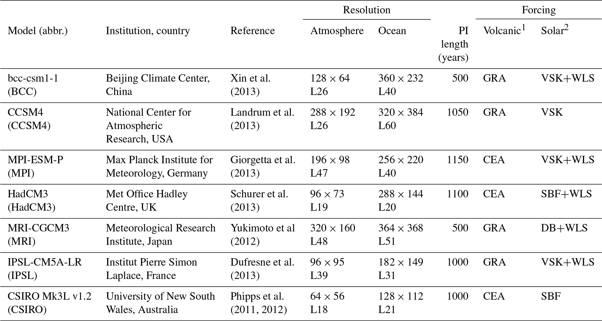
1 Volcanic forcings: GRA is Gao et al. (2008); CEA is Crowley et al. (2008). 2 Solar forcings: VSK is Vieira et al. (2011); DB is Delaygue and Bard (2011); SBF is Steinhilber et al. (2009); WLS is Wang et al. (2005).
2.1 Climate model simulations
We select models from CMIP5 (Taylor et al., 2012) that had provided output for all three experiments considered here: (i) pre-industrial control (PI) run with constant external forcing, (ii) last millennium (LM) and (iii) historical experiments with time-varying external forcings. Of the 10 GCMs that met this criterion, three models (MIROC, FGOALS, GISS) were excluded because they show a strong drift in the LM or PI simulations (Atwood et al., 2016; Fleming and Anchukaitis, 2016). Atwood et al. (2016) found long-term drift in global-mean surface air temperature in MIROC and FGOALS PI simulations, while Fleming and Anchukaitis (2016) found drift in GISS LM simulations during the initial several centuries and excluded these from their PDO analysis. Details of the remaining seven GCMs are summarised in Table 1 including the volcanic and solar forcings used. The forcing and boundary conditions for the LM simulations follow the protocols of Paleoclimate Model Intercomparison Project phase 3 (PMIP3), as suggested by Schmidt et al. (2011, 2012). The forcings are composed of volcanic aerosols, solar radiation, orbital variations, greenhouse gas (CH4, CO2 and N2O) concentrations and anthropogenic land-use changes over the period 850–1849. The historical simulations are forced with natural and anthropogenic forcing over the period 1850–2000. The comparison of these “forced” simulations with “unforced” control simulations provides a means of assessing what portion of the climate variability could be attributed to external forcing and what portion reflects purely internal variability. Also, these simulations are useful in providing a longer-term perspective for detection and attribution studies.
We interpolate output from all the models to the CCSM4 grid resolution to facilitate intercomparison. We note that the available model simulations were not necessarily continuous from their LM simulations into their historical simulations, so modes of variability cannot be calculated across 1850. Each model version was the same across all the simulations. Since our focus is on natural variability arising from internal and external causes, we have minimised the influence of any residual long-term drift or of anthropogenic transient forcings by first detrending (removing the linear trend) the LM (850–1849) and historical (1850–2000) time series separately and then merging them into a continuous detrended time series for the period 850–2000 (LMH hereafter). Our results are not sensitive to the linear detrending of the historical simulations (see Figs. S1 and S2 in the Supplement).
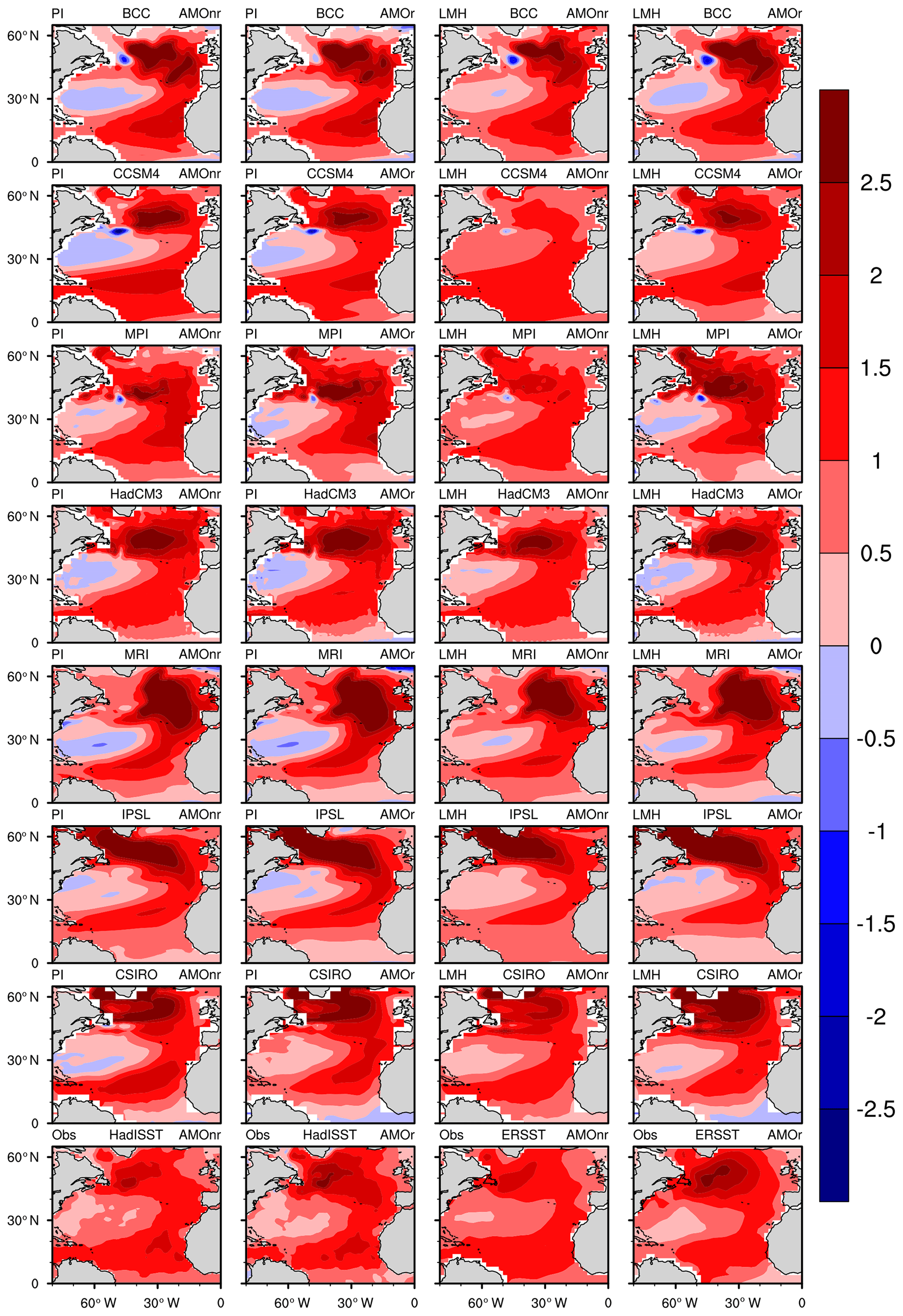
Figure 1AMO patterns defined by regression of annual-mean SST on the AMO index for each GCM for the PI (first and second columns) and LMH (third and fourth columns) experiments compared with HadISST and ERSST observation (bottom row). The first and third columns use the AMO index calculated without subtracting the global SST anomaly (AMOnr), while the second and fourth columns use the AMO index after subtracting the global SST anomaly (AMOr).
2.2 Diagnosing Atlantic and Pacific variability
The AMO and PDO time series are diagnosed using the same methods for both the model simulations and the instrumental observations. For the latter, we used HadISST (Rayner et al., 2003) and ERSST (Smith and Reynolds, 2004) for the periods 1871–2000 and 1854–2000, respectively.
The AMO index is calculated from the area-weighted North Atlantic (0–65∘ N, 80–0∘ W) monthly mean SST anomaly for the LMH and PI simulations. When the value of the index is positive (negative), it is known as the warm (cold) phase of the AMO. We have considered here two sets of AMO indices: with (hereafter AMOr) and without (hereafter AMOnr) first subtracting the global-mean SST anomaly time series (Trenberth and Shea, 2006) from the spatially averaged (North Atlantic) time series anomalies at each time interval. Atlantic SST will exhibit both internal variability and the response to external forcings (Wang et al., 2017); by subtracting the global-mean SST anomaly, the AMOr index will reflect more closely the variability that is focussed on the North Atlantic region and not the signal of external forcing present in the global SST pattern. The annual means of the AMO indices generated by the above two methods are regressed over the North Atlantic annual-mean SSTs (Fig. 1) to show the spatial pattern of the AMO; they closely agree with the observations (Fig. 1, bottom panels). See Flato et al. (2013) for a more detailed discussion of the simulated AMO in climate models.
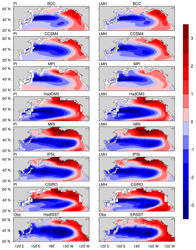
Figure 2PDO SST patterns defined by the first empirical orthogonal function (EOF) of annual-mean SST for each GCM for the PI (first column) and LMH (second column) experiments compared with the HadISST and ERSST observations (bottom row).
The PDO index is calculated as the leading mode from an empirical orthogonal function (EOF) analysis of annual SST anomalies in the North Pacific region (20–65∘ N, 110∘ E–110∘ W), which are calculated by first removing the long-term monthly means, then subtracting the monthly mean global SST anomaly at each time interval and then forming annual means. The methodology used to calculate PDO is similar to the methods discussed by Mantua et al. (1997), Landrum et al. (2013) and Fleming and Anchukaitis (2016). The EOF analysis yields spatial patterns (loadings) and temporal scores (time series). In its positive (negative) phase, SSTs are above (below) normal along the west coast of North America and below (above) average in the central North Pacific (Fig. 2). The simulated PDO patterns agree well with each other and with the observed pattern (Fig. 2, bottom panels), in terms of the position and strength of the loading maxima and main loading gradients. There are considerable differences in their time series, however, which are discussed later. The ability and limitation of CMIP5 models to simulate PDO characteristics are discussed by Flato et al. (2013).
The model-simulated AMO and PDO indices are generated using monthly mean SSTs for the LMH (850–2000) and PI simulations, and then converted into annual-mean (January–December) values for our analysis. Similarly, for the time series analysis of the temperature over East Asia (TAS), the annual-mean (January–December) value is calculated over the land grid points only and area averaged over the region of 10–55∘ N and 60–150∘ E. We also consider warm- (April–September) and cold-season (October–March) averages.
2.3 Paleoclimate and forcing reconstructions
The GCMs used volcanic forcing from either Gao et al. (2008; hereafter GRA) or Crowley et al. (2008; hereafter CEA) in their last millennium simulations (Table 1). Accordingly, we compare the model and reconstructed data with GRA and CEA, as well as with the newer volcanic forcing reconstruction from Sigl et al. (2015) (hereafter SIG). Table 1 also lists the solar forcing reconstructions used to drive the GCMs (hereafter VSK, DB and SBF) and we use these to identify the solar signal in the data.
Table 2Summary of the paleoclimate reconstructions considered in this study.
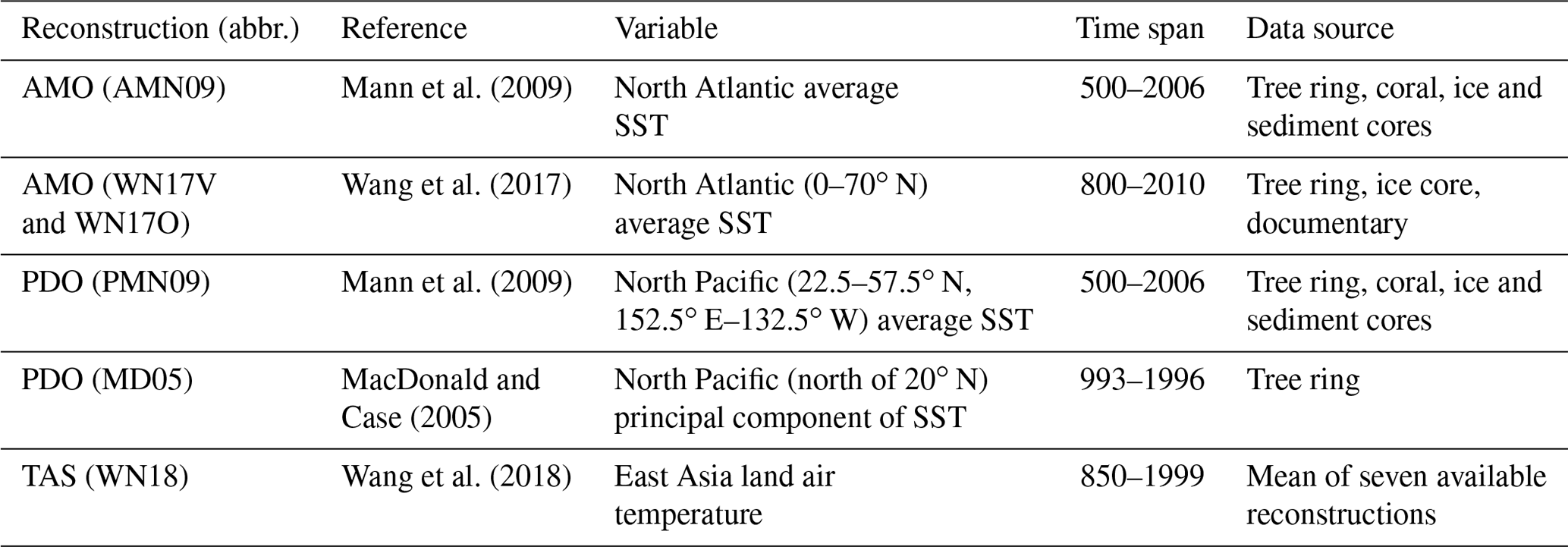
We used proxy-based reconstructions for the AMO, PDO and TAS as summarised in Table 2. We selected these reconstructions instead of alternatives because of the availability of the data for a period that covers at least 1000 years of our main analysis period (850–2000).
Two AMO reconstructions are used in this study. Mann et al. (2009) reconstructed near-global fields of surface temperature using a diverse mix of annual- and decadal-resolution tree-ring, coral, ice core and sediments records from across the globe. Their AMO series (hereafter AMN09) was computed from the North Atlantic SST grid cells of their reconstructed fields and extends for the period 500–2006 with 10-year low-pass filters. The annually resolved AMO by Wang et al. (2017) is based on tree-ring, ice core, historical records only from circum-Atlantic land regions and is available for the period 800–2010. Wang et al. (2017) first reconstruct Atlantic multidecadal variability (hereafter WN17V) and then subtract an estimate of the externally forced component (by regressing against solar and volcanic forcing) to obtain a series that represents mostly internal variability, denoted as the Atlantic Multidecadal Oscillation (hereafter WN17O). The two reconstructions (AMN09 and WN17V) provide estimates of the full (both external and internal) variability of the North Atlantic SST. Although Mann et al. (2009) reconstructed near-global SST fields, we have not subtracted the global-mean SST from the Atlantic-mean SST to isolate the internal AMO variability (compare the AMOr series from the models) because prior to 1600 their reconstruction is a linear combination of only two spatial patterns which gives limited information about the Atlantic–global SST difference.
One annual-mean PDO reconstruction is based on Mann et al. (2009) as described above and hereafter denoted as PMN09. This series is an average of SST grid cells over the central North Pacific region (22.5–57.5∘ N, 152.5∘ E–132.5∘ W): since this region has mostly negative loadings in our EOF-based PDO index (Fig. 2), we multiply PMN09 by −1 to make it comparable to the other PDO indices. Another annually resolved PDO index is from MacDonald and Case (2005; hereafter MD05), who used only tree-ring records from Pinus flexilis in California and Alberta to reconstruct PDO for the period 993–1996. The PDO reconstructions, unlike the EOF-based definition in modelled and observed SST datasets, might also contain some signal of external forcing because the proxy records are influenced by externally forced variability.
The East Asian temperature reconstruction for the warm season is from Wang et al. (2018; hereafter WN18), which uses the mean of seven published reconstructions and is available for the period 850–1999. See Wang et al. (2018) for a discussion of the underlying reconstructions and their similarities/differences. We repeat some of our analyses with three of the individual reconstructions used in the WN18 composite (Fig. S3).
It should be noted that the time sequences of the reconstructed and simulated data are not directly comparable because each will have its own realisation of internal variability. They should, however, be internally consistent so that their teleconnections can be compared on multidecadal timescales, along with any contribution that is externally forced (to the extent that the external forcing matches between the datasets).
2.4 Analysis methods
Since our focus is to understand climate variability on multidecadal timescales, all the time series are smoothed by a 30-year low-pass filter using the Lanczos filter. The correlation analyses are tested for statistical significance using a two-tailed Student's t test. The number of degrees of freedom is the number of 30-year long segments minus 2; i.e. a low-pass-filtered 1000-year long time series has 33 independent samples (1000/30) and 31 degrees of freedom. The null hypothesis (that the correlation is zero) is rejected if the correlation value is greater than the corresponding critical value: we test the statistical significance at the 95 % level for area means but lower this to 90 % at the grid-cell level because additional noise increases the risk of a type II error.
Spectral analysis of AMO and PDO indices is performed via the fast Fourier transform (FFT). In undertaking spectral analysis, we are interested in the overall shape of the spectra, their redness and broad multidecadal power, and whether these are similar between models, with/without forcing and between AMO index definitions. We are less interested in the apparent statistical significance of individual periodicities so we do not apply such a statistical test. In order to isolate the near-internal variability from the LMH model runs, in some analyses, we regress out the influence of volcanic forcing from the TAS, AMO and PDO time series by calculating the regression coefficient of the GRA or CEA volcanic global forcing time series against the TAS, AMO and PDO time series, respectively.
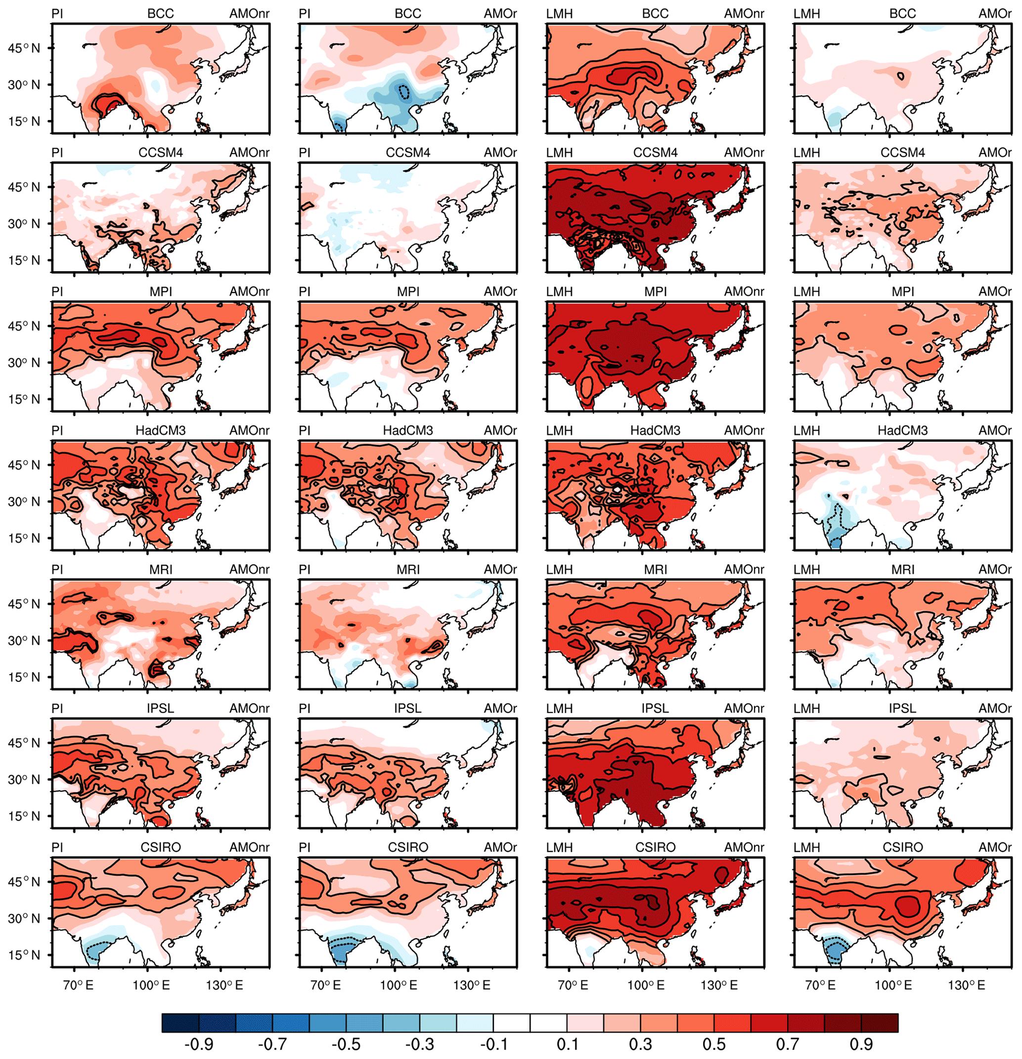
Figure 3Correlations between annual-mean East Asian surface temperatures and AMO index for each GCM for PI (first and second columns) and LMH (third and fourth columns) experiments. AMOnr and AMOr are the two definitions of AMO index as described in Fig. 1. Correlation values significant at 90 % levels using a two-tailed Student's t test are contoured.
Figure 3 shows the correlation between the AMO index and multidecadal variations in surface temperature in the LMH and PI simulations. The correlation with area-averaged East Asian surface temperature (TAS) is also calculated (Fig. 4). In the PI simulations with constant external radiative forcing, internal climate variability alone results in correlations between the AMOnr and East Asian temperature that are generally positive (Fig. 3, column 1); i.e. a warmer North Atlantic Ocean is associated with warmer East Asian temperatures. There is only widespread statistical significance on a grid-cell basis for four models (MPI, HadCM3, IPSL and CSIRO; Fig. 3, column 1), though correlations with area-averaged TAS are quite strong (multi-model mean > 0.5) and statistically significant for all models except BCC and CCSM4. The strength of the correlation is very sensitive to the presence of external forcing, becoming more strongly positive both spatially (Fig. 3, column 3) and on an area-averaged basis (Fig. 4) in the LMH run for all GCMs (all are significant and the multi-model correlation reaches 0.75). In many models, the strong positive correlation occurs mostly because natural external (e.g. volcanic eruptions) forcings cause concurrent warming or cooling in both the Atlantic and East Asian regions (Fig. 7). Indeed, including external forcings changes CCSM4 from having the weakest (and non-significant) correlation to having the strongest (0.84) correlation between the AMOnr and East Asian temperature.

Figure 4Correlations of annual-mean East Asian regional average surface temperature against AMO for each GCM (circles) for PI and LMH experiments compared with reconstructions (triangles). The mean correlations for the seven GCMs are marked with black circles connected by a solid line. AMOnr and AMOr are the two definitions of AMO index described in Fig. 1, while “vo” indicates that the volcanic influence on East Asian temperature has been removed by linear regression in the LMH experiments. The thick circles and triangles show values significant at 95 % level using a two-tailed Student's t test. The reconstruction correlations are between the WN18 East Asian temperature and the three AMO reconstructions (Table 2; the correlation with WN17O is weak (0.24) because it represents only internal AMO variability).
When we remove the global SST anomaly before calculating the AMO index, its association with TAS becomes much weaker. The reduction in correlation is especially large for LMH runs, both on a grid-cell basis (Fig. 3, column 3 vs. 4) and for area-averaged TAS (Fig. 4, AMOr vs. AMOnr). This is because much of the external forcing influence on North Atlantic SST also drives global SST, so subtraction of the global-mean SST anomaly prior to the calculation of the AMO removes this externally forced variability from the AMO. However, because TAS has a different sensitivity to global forcings, its correlation with AMOr is decreased but remains significant for some models (MPI, MRI and CSIRO). Comparing the correlations with the AMOr index, we see that the correlation is notably weaker in the LMH run than in the PI run for the MPI, HadCM3 and IPSL models (Figs. 3 and 4). This is because the forcings generate a response in the TAS but not in the AMOr (any response is mostly removed because global SST is subtracted from Atlantic SST), weakening their correlation. MRI and CSIRO are notable in that their TAS correlations with AMOr are stronger in the LMH run than in the PI run; this could arise if the amplitude of SST response is greater in the Atlantic than in their global mean, so that AMOr still retains an external forcing signal that then correlates with the external forcing signal in East Asian TAS.
In summary, four models show a clear association between the AMO and East Asian temperatures (especially in the northern half of the region considered here) that arises from internal variability (i.e. in the PI run) and remains significant even if the global SST anomaly is subtracted. This suggests that this mode of internal variability only partly projects onto global-mean SST anomalies. Furthermore, the correlations for all models are strongly affected (increased) by the inclusion of external forcing unless the AMO is defined by subtracting the global-mean SST from the Atlantic SST.
These dependencies of the model correlations on the presence of external forcing and on the calculation of the AMO index are important in the context of interpreting reconstructed data. Suppose we wish to use reconstructed data to answer the following question: does the AMO, as a mode of internal variability, influence East Asian temperatures on multidecadal timescales? The reconstructions represent the real world (a situation with external forcings) and some AMO reconstructions (e.g. AMN09 and WN17V) have not isolated internal variability of the North Atlantic SST from externally forced signals (because, for instance, global-mean SST cannot be subtracted before calculating the AMO if global SST has not been independently reconstructed). This situation is equivalent to column 3 of Fig. 3 (LMH runs with AMOnr indices) and a strong positive correlation might be found between the AMO and East Asian temperatures – but this would not establish that the AMO, as a mode of internal climate variability, was strongly influencing East Asian temperatures on multidecadal timescales.
The WN18 East Asian reconstruction represents warm-season temperature, so we repeated our model analysis but using both warm- and cold-season temperatures and obtained results that are closely consistent with those using annual-mean temperatures. The reconstructed AMO series all show positive correlations with the WN18 East Asian temperature reconstruction (Fig. 4). Those representing full AMO variability (WN17V and AMN09) have correlations around 0.4, while the correlation with East Asian temperature falls to 0.24 (which is not significant) for the WN17O series representing only internal AMO variability. None of the reconstructed AMO or East Asian surface temperature series correlate significantly with the equivalent simulated series from the LMH runs, indicating that internal variability and any errors in reconstructed climate and forcings dominate the influence of external forcing, or that model response to forcings is unrealistic.
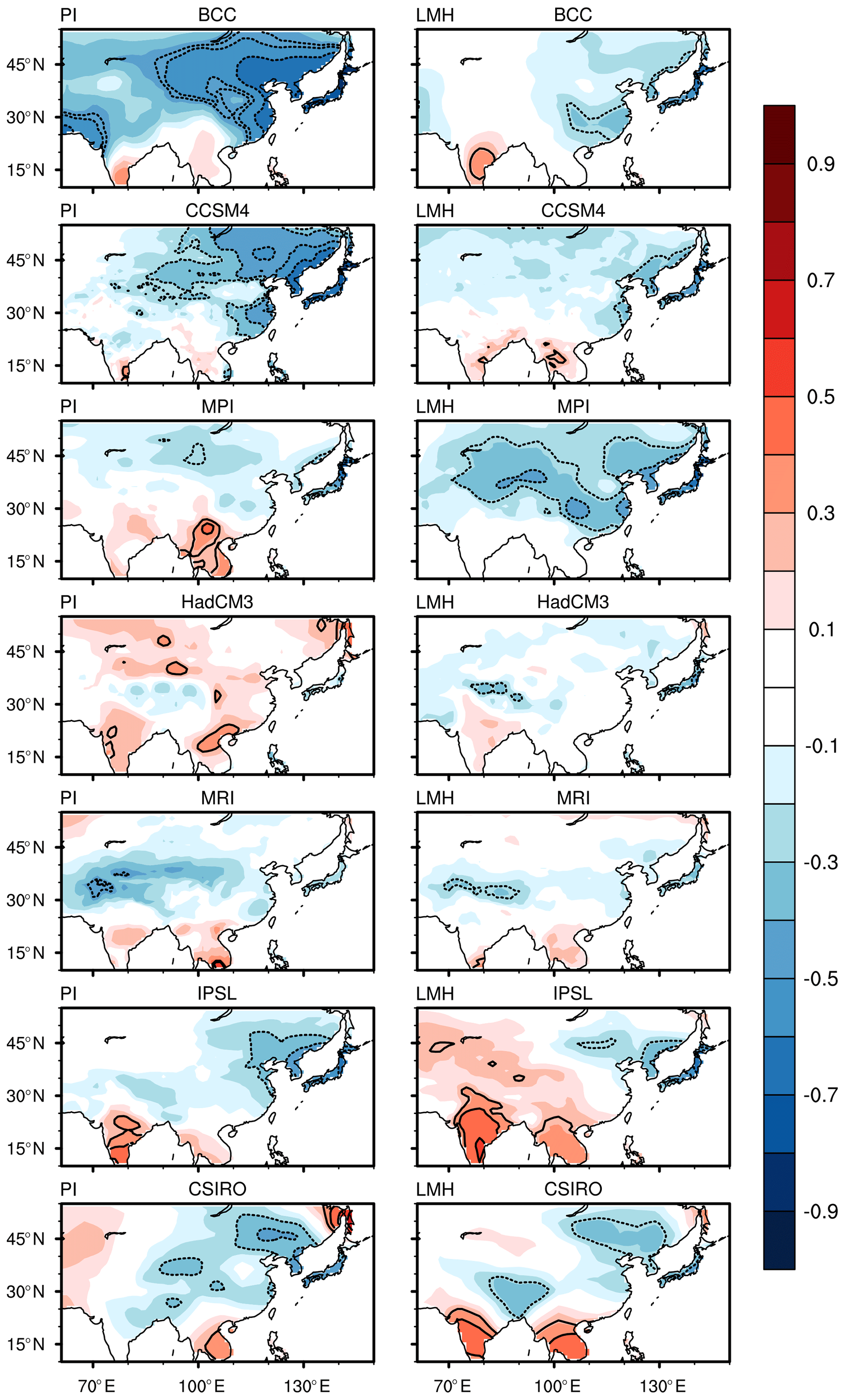
Figure 5Correlations between annual-mean East Asian surface temperatures and PDO index for each GCM for PI (first column) and LMH (second column) experiments. Correlation values significant at 90 % levels using a two-tailed Student's t test are contoured.
Similar to the AMO analysis, Figs. 5 and 6 show the correlation between PDO and TAS. The PDO is negatively correlated with TAS in Japan, as expected because cooler SSTs lie adjacent to this region when the PDO index is positive (Fig. 2). These negative correlations extend from Japan across large parts of the northeast of our region in four (BCC, CCSM4, IPSL and CSIRO) out of seven models, though they vary widely in strength and significance between models and are mostly weakened by the inclusion of external forcing (LMH; compare PI in Fig. 5). Most models (for both the PI and LMH runs) show a dipole with mainly negative correlations in the north or centre of our region and positive correlations in the south (e.g. parts of India and southeast Asia). The predominance of negative correlations across the spatial field means that six out of seven models simulate a negative correlation between area-averaged TAS and PDO, though few are significant because we are averaging across regions with opposite correlations (Fig. 6). There are two key differences between the results with and without external forcing. First, the correlations weaken when external forcing is applied to the models (except for the MPI model where it was already weak). Second, the spread in results is much wider in the absence of forcing (with significant negative correlations for BCC and CCSM4). Together, these results suggest that the internal-variability teleconnection between PDO and East Asian temperature is very model dependent but that external forcing consistently weakens the association. The weakening is likely because the forcing drives additional variability in East Asian temperatures but not in the PDO (because we subtract the global-mean SST anomaly prior to calculating it and use an EOF definition that represents SST spatial differences rather than mean SST across the North Pacific; Fig. 2). Using this definition (rather than a simple area-mean SST), the model PDOs do not have strong or consistent responses to forcing in the LMH simulations, in agreement with Landrum et al. (2013) and Fleming and Anchukaitis (2016).
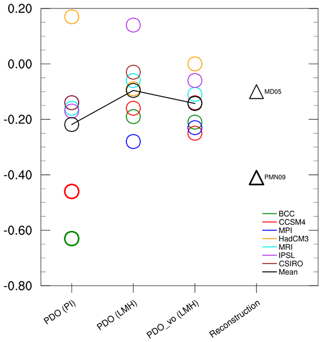
Figure 6Correlations of annual-mean East Asian regional average surface temperature against PDO index for each GCM (circles) for PI and LMH experiments compared with reconstructions (triangles). The mean correlations for the seven GCMs are marked with black circles connected by a solid line; “vo” indicates that the volcanic influence on East Asian temperature has been removed by linear regression in the LMH experiments. The thick circles and triangles show values significant at 95 % level using a two-tailed Student's t test. The reconstruction correlations are between the WN18 East Asian temperature and the two PDO reconstructions (Table 2).
We have also compared the reconstructed PDO and TAS time series (Fig. 6). The correlations are also negative: MD05-WN18 and PMN09-WN18 are −0.10 and −0.41, respectively, but only the latter is significant. The weak correlation with MD05 might be partly related to the fact that this reconstruction is based on only two tree-ring records of North America, suggesting more uncertainty if teleconnection patterns it relies on change through time. The simulated PDO series show very weak correlations with the reconstructed PDO series: as with the AMO, this implies that an external forcing influence is weak compared with internal variability and reconstruction errors, or that models' PDO response to forcings is unrealistic. For the simulated PDO indices, any external forcing influence may be weak if the PDO calculation (an EOF analysis with the global-mean SST removed) effectively removes a forcing signal. As before, we repeated our model analysis using both warm- and cold-season East Asian temperatures and found very similar results to the annual temperatures.
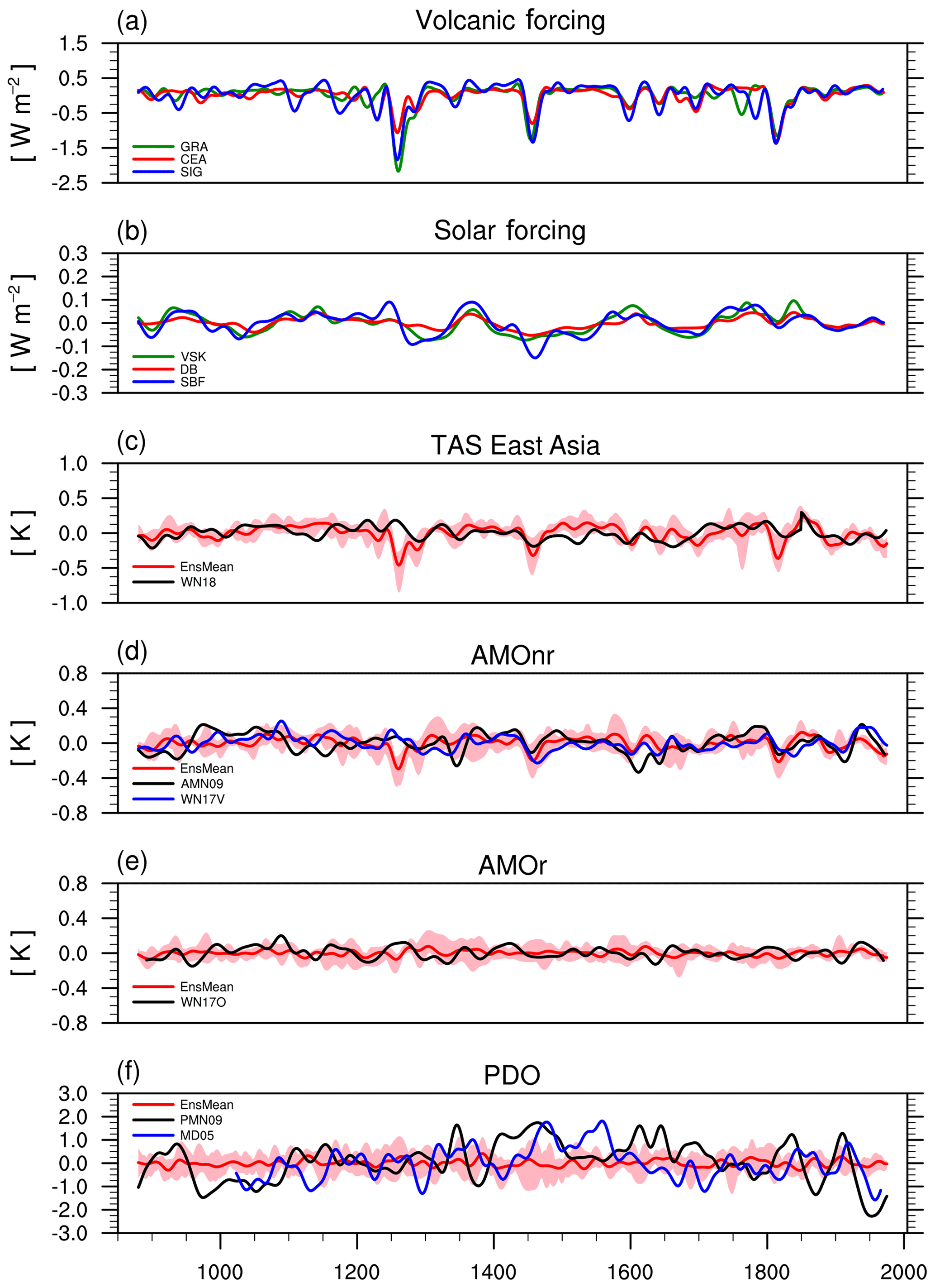
Figure 7Time series of (a) volcanic forcing, (b) solar forcing, (c) surface temperature over East Asia, (d) AMO index without subtracting the global SST (AMOnr), (e) AMO index after subtracting the global SST (AMOr) and (f) PDO index; all are annual-mean values, passed through a 30-year low-pass filter and truncated to remove filter end effects. Model simulations in panels (c)–(f) are given as the mean (red line) and spread (pink shading) of the seven GCMs. Model simulations for surface temperature, AMO and PDO are compared with the available reconstructed data (black and blue lines).
The behaviour of the AMO and PDO time series and their correlation with East Asian temperature are clearly sensitive to the presence of external forcing (e.g. LMH vs. PI differences), so we now consider the effect of volcanic and solar forcings. Volcanic forcing is the largest external influence within the LM runs (Atwood et al., 2016) and is a key driver of the Little Ice Age and other cooling periods during the last millennium (Briffa et al., 1998; Ammann et al., 2007; Atwood et al., 2016). However, Wang et al. (2018) showed that their East Asian temperature reconstruction has significant correlations with solar forcing reconstructions. So, we have compared the model simulations and reconstructions to both volcanic (GRA, SEA and SIG; Fig. 7a) and solar forcing (VSK, DB and SBF; Fig. 7b). All three volcanic forcing time series (GRA, CEA and SIG) are closely correlated with each other but are by no means identical (Fig. 7a). For the period AD 850–2000, their correlations range from 0.75 to 0.82 (for pairs of GRA, CEA and SIG volcanic forcing) and from 0.80 to 0.91 (for pairs of VSK, DB and SBF solar forcing), highlighting the value in considering multiple forcing histories.
Visually, it is clear to see that the simulated East Asian temperatures and AMOnr time series display a multidecadal association with volcanic forcing, while AMOr and PDO time series do not (Fig. 7). The colder climate over East Asia and the Atlantic (i.e. AMOnr) is especially evident during the three periods containing strong eruptions (1250s, 1450s and 1810s). Potential influences of solar forcing are harder to identify because the forcing is weaker and shows less distinct episodic behaviour than the volcanic forcing. Turning to correlations (Fig. 8), some key behaviours are clear, as discussed below.
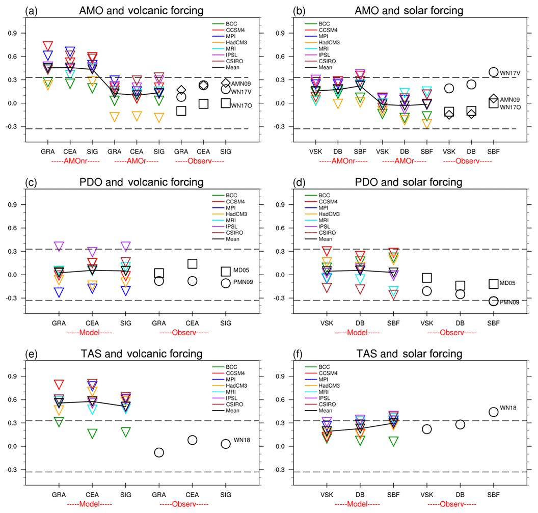
Figure 8The correlations of annual-mean AMO, PDO and TAS with volcanic forcing (a, c, e) and solar forcing (b, d, f) for each GCM (triangles) and reconstruction (circle, square and diamond). The threshold values for the individual correlations significant at 95 % level using a two-tailed Student's t test are marked as dashed lines. The means of the seven model correlations are shown by black triangles connected by black lines.
First, simulated East Asian temperature is positively correlated with volcanic forcing (significant for all models except BCC) but this is not the case for reconstructed temperatures (on these multidecadal timescales at least; WN18 also report that the volcanic signal is small compared with other influences). We tested to see if the latter result was due to our use of the Wang et al. (2018) composite of reconstructions, rather than some individual reconstructions that might better resolve the response to volcanoes, but obtained similar results (Fig. S3). East Asian temperatures are also positively correlated with solar forcing but these are weaker than with volcanic forcing and are either insignificant or marginally significant for all models and reconstructions.
Second, simulated AMOnr time series are more strongly (positively) correlated with external forcings than are the AMOr time series. With volcanic forcing, the AMOnr correlations are significant for all models except BCC (mean correlations between 0.4 and 0.5 with all three volcanic forcing datasets), while with solar forcing the model correlations are typically between 0.0 and 0.3. Removing the global-mean SST prior to calculating the AMO (i.e. AMOr) reduces the correlations with both volcanic and solar forcing (Fig. 8). The reconstructed WN17O series is not expected to correlate with external forcings because Wang et al. (2017) removed a regression estimate of the forced signal in reconstructed Atlantic SST to obtain this series. The other two reconstructions (WN17V and AMN09), however, also show only weak correlations with the external forcings.
Third, the simulated and reconstructed PDO time series do not correlate significantly with either volcanic or solar forcing (with a couple of exceptions that might be expected by chance – the IPSL model with volcanic forcing and the PMN09 reconstruction with SBF solar forcing). The means of the model correlations are close to zero.
These results explain some of the earlier findings concerning influences on East Asian temperature, specifically that external forcing strengthens its positive relationship with the AMO but weakens its (generally negative) relationship with PDO. Strong positive correlations demonstrate that natural external forcings cause concurrent warming or cooling in both the Atlantic and East Asian regions, contributing to the strengthening of positive correlations between AMOnr and TAS in the LMH simulations compared with the PI runs (Figs. 3 and 4). Removing the global SST anomaly first to obtain the AMOr index renders the correlations with volcanic forcing insignificant (Fig. 8) and the AMOr time series (Fig. 7e) do not show any cooling with corresponding volcanic forcing eruptions. This contributes to the much-reduced correlations with TAS when the AMOr series are used (Figs. 3 and 4).
In terms of Pacific variability, the PDO is not strongly correlated with external forcing (as expected because it is diagnosed as an EOF of SST anomalies having first subtracted the global-mean SST). Therefore, adding external forcing does not greatly affect the PDO but it does cause additional variability in East Asian temperature, thus weakening the negative PDO–TAS relationship (Figs. 5 and 6; correlation measures the relative strength of their common variability). We might expect this effect to be particularly noticeable in those models that simulate a strong positive correlation between East Asian TAS and volcanic forcing (Fig. 8e). This is the case for CCSM4 (strong volcanic signal in TAS, adding the external forcing greatly weakens the PDO–TAS relationship) but not for MPI (strong volcanic signal in TAS but the PDO–TAS relationship is stronger in LMH than in PI, probably because this model has a negative PDO–volcanic correlation) nor BCC (the PDO–TAS relationship is weaker in LMH than in PI despite there being little influence of volcanic and solar forcings on East Asian temperature in this model).
Since we can diagnose AMO and PDO time series that are not significantly correlated with volcanic forcing (Fig. 8: AMOr and the EOF-based PDO), we further tried factoring out the volcanic influence from the TAS time series to see if we could reproduce the behaviour of the control runs (PI) using data from the forced runs (LMH). This is akin to trying to identify the behaviour of internal variability in the real Earth system (Steinman et al., 2015; Dai et al., 2015). We regressed volcanic forcing (using the series for each model; Table 1) on the TAS data and removed it to yield a TAS series without the linear influence of the volcanic forcing (see Sect. 2.4). We note that volcanic eruptions may have lagged effects on the oceans from years to decades (e.g. Pausata et al., 2015) and zero-lag regressions may not fully account for this kind of impact on the climate system.
Factoring out volcanic forcing from TAS did weaken the correlations with the simulated AMO LMH series (Fig. 4; AMOnr vs. AMOnr_vo for LMH), so that the mean of the model correlations was very close to that found during the PI runs. However, the TAS–AMOnr correlations for most individual models differ between PI and the LMH with volcanic influenced factored out. Similar results are found using the AMOr index: there is agreement between PI and LMH correlations for the mean of the model correlations but not for the individual models (e.g. of the four models that show significant positive correlations in the PI runs, only two are significant in the LMH runs with volcanic influence on TAS factored out). Despite factoring out the influence of the dominant forcing and using an AMO index that is not strongly correlated with forcing, we still find very different behaviour in the PI simulation than in the LMH simulation. For two models (BCC and CCSM4), we correctly infer the small role of AMO internal variability on East Asian TAS from the LMH run; for two models (MPI and CSIRO), we correctly infer a significant AMO role (though underestimating its importance for MPI); for two models (HadCM3 and IPSL), we fail to find the significant AMO role; and for MRI, we find a significant AMO role despite its PI run showing no significant AMO role on East Asian TAS.
Factoring out the volcanic signal hardly changes the simulated relationships between East Asian TAS and the PDO (PDO_vo; Fig. 6). For some models, therefore, we are not able to determine the internal variability teleconnection between PDO and TAS when external forcings are present despite using a PDO definition that is insensitive to external forcing and regressing out the volcanic influence on TAS. This outcome is especially clear for the two models (BCC and CCSM4) whose internal variability shows strong, significant associations between PDO and East Asian TAS but correlations are weak and insignificant in their LMH runs.
In the BCC model, the relationship between volcanic forcing and both AMO and East Asian TAS is notably weaker than the other models (Fig. 8). This behaviour is the same if we use warm- or cold-season TAS (not shown) rather than annual-mean TAS. The smaller influence of volcanic forcing for BCC partly explains why it has the weakest correlation between TAS and AMOnr during the LMH simulations. To explore this weak BCC response to volcanic eruptions, we analyse net incoming shortwave radiation anomalies composited for the three largest volcanic eruption events in all models (Fig. 9). This shows that the decrease in net incoming shortwave radiation following these eruptions in BCC is less than 25 % of the response in both CCSM4 and MPI. The other four models lie between BCC and MPI. We also have analysed the same for the major volcanic events during the historical period for BCC, CCSM4 and MPI but did not find such a weak BCC response compared to the other two models. The weak volcanic forcing and response in BCC may be an artefact of how they implemented volcanic forcing in their last millennium simulation.
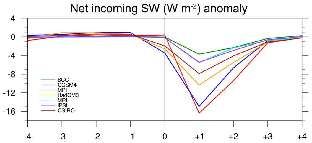
Figure 9Annual-mean composite anomaly of net shortwave (SW) radiation at the top of the atmosphere for three large volcanic eruption events for each GCM. Individual GCM results are aligned so that their peak negative SW anomalies occur at year+1 (i.e. 1258, 1452, 1815 for BCC, CCSM4, IPSL; 1258, 1452, 1816 for MRI; 1258, 1456, 1816 for MPI, HadCM3, CSIRO).
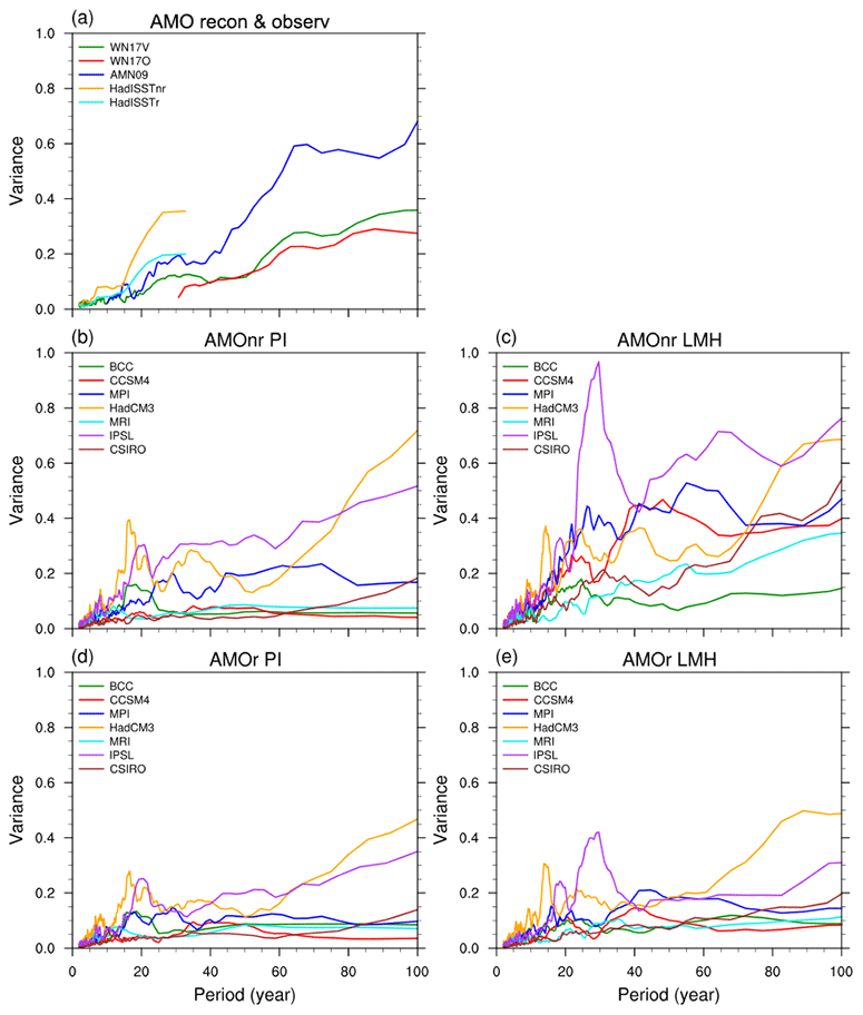
Figure 10Spectra of AMO index of reconstructions and instrumental data (a) and each of seven GCMs for PI (b, d) and LMH (c, e) experiments. AMOnr and AMOr are the two definitions of AMO index described in Fig. 1. Spectra are not shown for timescales that the underlying data cannot adequately represent (not for < 30 years for WN17O and not for < 10 years for AMN09 because these reconstructions use 30-year and 10-year low-pass-filtered data, respectively, and not for > 30 years for HadISST because the instrumental data are too short to determine power on longer timescales).
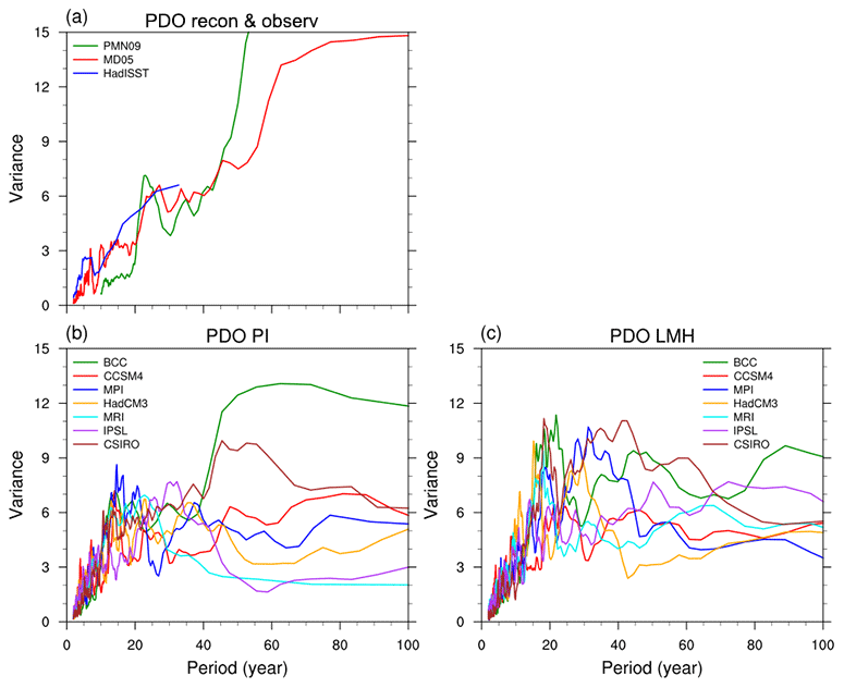
Figure 11Spectra of PDO index of reconstructions and instrumental data (a) and GCMs for PI (b) and LMH (c) experiments. Spectra are not shown for timescales that the underlying data cannot adequately represent (not for < 10 years for PMN09 because this reconstruction uses 10-year low-pass-filtered data, and not for > 30 years for HadISST because the instrumental data are too short to determine power on longer timescales).
To assess the role of external forcing further, the power spectra of the AMO and PDO indices are analysed (Figs. 10 and 11, respectively) using the annual-mean data (i.e. the data have not been low-pass filtered before spectral estimation) for the PI and LMH experiments, reconstructions and instrumental data. All AMO time series have red spectra (Fig. 10) at short timescales (up to 20 years) but at multidecadal timescales the redness, the absolute power and the presence of enhanced power across a broad range of frequencies all depend on the model, the presence/absence of forcing and the choice of AMO index. For the AMOnr index, the inclusion of external forcing (LMH runs) greatly strengthens the multidecadal power of the variability; the increase is more moderate for BCC (see earlier discussion). Removing the global-mean SST first (AMOr) reduces the difference between the PI and LMH runs. Some models (BCC, HadCM3 and IPSL) show enhanced power at about 20 years, and there is prominent power around 30 years in the forced IPSL simulation (LMH) that is partly reduced using the AMOr index. In the reconstructions, the spectra have steep gradients over the 40- to 60-year timescales, with elevated power above 60 years. In most models, variability around 60–80 years, often considered typical for the AMO, is quite strong but only MPI has power that is notably enhanced relative to the rest of its spectrum (CCSM4 has elevated power around 40–50 years). The AMO-reconstructed spectra provide a comparison (Fig. 10a) of the overall spectral shape. The MPI, HadCM3 and IPSL models have the reddest spectra, and for AMOnr LMH these are qualitatively similar to the spectra of the WN17V and AMN09 reconstructions, while the other models show much less multidecadal power.
In the case of the PDO, all models show red spectra with enhanced power at ∼15–20 years for both PI and LMH simulations, indicating that the Pacific variability arises mostly by internal variability. Landrum et al. (2013) found the same frequency for both control and last millennium simulations of the CCSM4 model. The enhanced PDO power at ∼15–20 years is filtered out by the 30-year smoothing used for the majority of analyses for reconstructions and models reported here, which might weaken the PDO–TAS correlation.
In this study, we identify the key teleconnections between the AMO, PDO and East Asian temperature in climate models on multidecadal timescales and determine to what extent external forcings affect these simulated teleconnections. The instrumental record is too short to clearly distinguish contributions from natural internal variability, natural external forcings and anthropogenic forcings at multidecadal timescales. Zhang et al. (2018) and Wang et al. (2018) have explored this issue using paleoclimate reconstructions of temperatures over a large region in East Asia. Here, we complement these studies by using the dynamical information provided by seven climate models (Table 1), with and without the influence of external forcings over the last millennium. Our key findings are as follows:
-
The models simulate multidecadal modes of variability in the extratropical oceans (AMO and PDO) with spatial patterns similar to those previously identified in the observations and proxy-based reconstructions. Using commonly applied methods to diagnose their time series (area-averaged North Atlantic SST for the AMO and the leading EOF of North Pacific SST for the PDO), we find that they have spectra with enhanced multidecadal variability similar to those found in observations and reconstructions (Figs. 10 and 11). However, the shape and amplitude of their spectra differ between the models and depend on the presence or absence of external forcing. Similar results were also reported by Parsons et al. (2017) and Fleming and Anchukaitis (2016).
-
These multidecadal modes of variability, along with variations in volcanic forcing, are found to influence East Asian temperature in the models. In most cases, East Asian temperature is positively correlated with the AMO and volcanic forcing, and negatively correlated with the PDO. The correlations are not spatially uniform, with PDO correlations strongest in the parts of the East Asian region that are closest to the extratropical North Pacific Ocean, and the AMO influence showing some latitudinal structure in most models.
-
The presence of external forcing strongly affects the apparent teleconnections between these multidecadal modes of variability and East Asian temperature. The effect depends on how the modes of variability are diagnosed and whether the forcings add common variability to both series (e.g. in the case of AMO) or add distinct variance to East Asian temperature but not to the mode of variability (e.g. in the case of PDO).
-
If the AMO is defined simply as the mean North Atlantic SST, then external forcing strengthens the AMO–East Asian temperature correlation by causing concurrent warming or cooling in both the Atlantic and East Asian regions. For all seven models, the correlations between East Asian temperature and the AMO are stronger in the last millennium forced simulation than in their corresponding control runs when the AMO is defined this way.
-
Defining the AMO as the difference between North Atlantic and global-mean SST reduces the effect mentioned in point 4 above because part of the externally forced signal is present in both SST series and the forced signal is reduced by computing their difference. The external signals in North Atlantic and global-mean SST are not identical, however, so using this AMO definition still does not yield correlations between East Asian temperature and the AMO that match those present in the model control runs. We still find different behaviour in the PI simulation than in the LMH simulation even if we also factor out the influence of the dominant forcing (volcanic) on East Asian temperature and use an AMO index that is not strongly correlated with forcing.
-
The PDO definition used here (the leading EOF of Pacific SST minus global-mean SST) yields an index that has only weak correlations with external forcing. Despite this, the multidecadal correlation between the PDO and East Asian temperature (which is negative) is still sensitive to the presence of external forcing. In this case, external forcing weakens the apparent teleconnection in two of the models, partly because external (especially volcanic) forcing generates a response in East Asian temperature but not in the PDO index, thus weakening the correlation between them. Regressing out the influence of volcanic forcing on East Asian temperature has limited effect on the correlation, which remains much weaker than in the control run for two of the models.
-
These results have significant implications for attempts to determine the influence of the AMO and the PDO strictly as modes of internal variability on East Asian temperatures. With models, we can simply analyse their control runs. For the real world, we do not have that option: we can analyse only reconstructions from a real world in which natural external forcings are present. In this case, we recommend, on the basis of our results, that careful consideration be given to separating out the influence of external forcings on both the indices of modes of variability and on the East Asian temperature series before determining the internal variability teleconnections.
There are a number of ways to separate internal and external variability, each with limitations. The modes of variability might be defined using the difference between regional and global SST. For example, the Last Millennium Reanalysis (Tardiff et al., 2019) provides globally complete temperature fields that could be used (though these are not independent of the CCSM4 climate model or the forcings used). In many cases, an independent reconstruction of global SST may not be available. Mann et al. (2009) reconstructed a global field of SST but prior to 1600 their reconstruction is a linear combination of only two spatial patterns which gives limited information about the Atlantic–global SST difference. Another approach is to identify and remove the influence of external forcing, e.g. by regression against forcing histories in reconstructions (Wang et al., 2017, 2018), by a method combining observations with an ensemble of coupled climate model simulations (Dai et al., 2015; Steinman et al., 2015) or using more sophisticated detection and attribution methods (e.g. Hegerl and Zwiers, 2011). These approaches require accurate forcing histories. A further approach is to use an EOF-based definition of the index where the spatial pattern has regions with loadings of opposite sign. External forcing tends to project similarly onto regions with opposite signs, cancelling out much of its influence on the resulting index. This is appropriate for the PDO, as used here, but less so for the AMO because the associated SST pattern is dominated by anomalies of the same sign (Fig. 1). Regression against forcing histories can also be used to remove the influence of external forcing on the target region (East Asian temperature for this study) prior to identifying the influence of AMO and PDO variability (Wang et al., 2018).
Even if these approaches are taken, it may still be impossible to determine the influence of multidecadal internal variability by analysing data that have been subject to external forcings. Despite factoring out the influence of the volcanic forcing in the AMO index, we still find different behaviour in the forced simulation than in the control run for some models. For example, in the forced run of the MPI model, the apparent AMO teleconnection on East Asian temperature is only 0.4 (AMOr_vo in Fig. 4), whereas in the control run it is strong (> 0.7 for AMOnr). For the BCC and CCSM4 models, we can correctly infer from the forced run that AMO internal variability has only a small influence on East Asian temperature provided we define the AMO as the difference between Atlantic and global SST (just factoring out the influence of external forcings from East Asian temperature is insufficient). Similar limitations were found regarding the PDO teleconnection: the PDOs in two models (BCC and CCSM4) have strong negative correlations with East Asian temperature but we cannot correctly diagnose this behaviour if we use a simulation with external forcings. We note the possibility that external forcing may have modified the dynamical behaviour of the internal variability in these cases, confounding the notion that we can clearly separate forced change from internal variability.
Finally, we found only partial agreement between the behaviours shown by the reconstructions and models. The correlations between East Asian temperature and the AMO and PDO showed the same signs in the models and the data, but the correlation values had a wide range. The strong influence of volcanic forcing in six of the models was not found in the reconstructions (Wang et al., 2018). We need to be careful while interpreting the results of the CMIP5-PMIP3 last millennium simulations in light of the paleoclimate record, because large uncertainties exist in the characterisation of volcanic forcing, reconstruction of aerosol loading, optical depth and aerosol effective radius as a function of time, latitude and height in the atmosphere, all of which exert important controls on the climate system (Atwood et al., 2016).
Results for individual Coupled Model Intercomparison Project Phase 5 (CMIP5) models (Taylor et al., 2012) are available for download from the database at https://esgf-node.llnl.gov/search/cmip5/ (last access: 15 June 2019). The instrumental SST data for HadISST (Rayner et al., 2003) and ERSST (Smith and Reynolds, 2004) are available from https://www.metoffice.gov.uk/hadobs/hadisst/ (last access: 1 June 2019) and https://www.esrl.noaa.gov/psd/data/gridded/data.noaa.ersst.v5.html (last access: 1 June 2019), respectively. Volcanic forcing (Gao et al., 2008; Crowley et al., 2008) and solar forcing (Vieira et al., 2011; Delaygue and Bard, 2011; Steinhilber et al., 2009; Wang et al., 2005) data are available as a supplementary data file from https://doi.org/10.5194/gmd-5-185-2012 (Schmidt et al., 2012). The other volcanic forcing data by Sigl et al. (2015) are available as supplementary information at https://doi.org/10.1038/nature14565. The AMO and PDO data by Mann et al. (2009) are available as supporting online material from https://doi.org/10.1126/science.1177303. The Atlantic multidecadal variability (AMV) and AMO data by Wang et al. (2017) are available at https://www.ncdc.noaa.gov/paleo-search/study/22031 (last access: 10 June 2018). The East Asian surface temperature composite data by Wang et al. (2018) are available at https://www.ncdc.noaa.gov/paleo-search/study/27372 (last access: 15 June 2019). The PDO data by MacDonald and Case (2005) are available at https://www.ncdc.noaa.gov/paleo-search/study/6338 (last access: 10 February 2018). The other summer temperature reconstructions for East Asia used in our supplementary material are from Cook et al. (2013) (https://www.ncdc.noaa.gov/paleo/study/19523; last access: 5 January 2019), Shi et al. (2015) (https://www.ncdc.noaa.gov/paleo/study/18635; last access: 5 January 2019) and Zhang et al. (2018) (https://www.ncdc.noaa.gov/paleo-search/study/23491; last access: 5 January 2019).
The supplement related to this article is available online at: https://doi.org/10.5194/cp-15-1825-2019-supplement.
TJO designed the study. The data analysis was led by SBR with contributions from TJO and MJ. All the figures are made by SBR. BY and JW provided the East Asian temperature reconstruction data and contributed to discussion of the results. All authors contributed to the writing of the paper.
The authors declare that they have no conflict of interest.
Support provided by the Belmont Forum and JPI-Climate project INTEGRATE (An Integrated data–model study of interactions between tropical monsoons and extratropical climate variability and extremes). We are thankful to two anonymous referees whose constructive comments helped to improve our study.
This research has been supported by the Natural Environment Research Council (grant no. NE/P006809/1), the National Key R&D Program of China (grant no. 2017YFA0603302) and the National Science Foundation of China (grant no. 41661144008).
This paper was edited by Zhengtang Guo and reviewed by two anonymous referees.
Ammann, C. M., Joos, F., Schimel, D., Otto-Bliesner, B., and Tomas, R.: Solar influence on climate during the past millennium: Results from transient simulations with the NCAR Climate System Model, P. Natl. Acad. Sci. USA, 104, 3713, https://doi.org/10.1073/pnas.0605064103, 2007.
Atwood, A. R., Wu, E., Frierson, D. M. W., Battisti, D. S., and Sachs, J. P.: Quantifying climate forcings and feedbacks over the last millennium in the CMIP5-PMIP3, J. Climate, 29, 1161–1178, 2016.
Briffa, K. R., Jones, P. D., Schweingruber, F. H., and Osborn, T. J.: Influence of volcanic eruptions on Northern Hemisphere summer temperature over the past 600 years, Nature, 393, 450–455, 1998.
Buckley, B. M., Ummenhofer, C. C., D'Arrigo, R. D., Hansen, K. G., Truong, L. H., Le, C. N., and Stahle, D. K.: Interdecadal Pacific Oscillation reconstructed from trans-Pacific tree rings: 1350–2004 CE, Clim. Dynam., 53, 3181–3196, https://doi.org/10.1007/s00382-019-04694-4, 2019.
Buntgen, U., Tegel, W., Nicolussi, K., McCormick, M., Frank, D., Trouet, V., Kaplan, J. O., Herzig, F., Heussner, K.-U., and Wanner, H.: 2500 years of European climate variability and human susceptibility, Science, 331, 578–582, 2011.
Christiansen, B. and Ljungqvist, F. C.: Challenges and perspectives for large-scale temperature reconstructions of the past two millennia, Rev. Geophys., 55, 40–96, 2017.
Coats, S. and Smerdon, J. E.: Climate variability: The Atlantic's internal drum beat, Nat. Geosci., 10, 470–471, 2017.
Coats, S., Smerdon, J. E., Cook, B. I., and Seager, R.: Stationarity of the tropical Pacific teleconnection to North America in CMIP5/PMIP3 model simulations, Geophys. Res. Lett., 40, 4927–4932, 2013.
Cook, E. R., Krusic, P. J., Anchukaitis, K. J., Buckley, B. M., Nakatsuka, T., and Sano, M.: Tree-ring reconstructed summer temperature anomalies for temperate East Asia since 800 C.E., Clim. Dynam., 41, 2957–2972, 2013.
Crowley, T. J., Zielinski, G., Vinther, B., Udisti, R., Kreutz, K., Cole-Dai, J., and Castellano, E.: Volcanism and the Little IceAge, PAGES Newslett., 16, 22–23, 2008.
Dai, A., Fyfe, J. C., Xie, S.-P., and Dai, X.: Decadal modulation of global surface temperature by internal climate variability, Nat. Clim. Change, 5, 555–559, 2015.
Delaygue, G. and Bard, E.: An Antarctic view of Beryllium-10 and solar activity for the past millennium, Clim. Dynam., 36, 2201–2218, https://doi.org/10.1007/s00382-010-0795-1, 2011.
Delworth, T. L. and Mann, M. E.: Observed and simulated multidecadal variability in the Northern Hemisphere, Clim. Dynam., 16, 661–676, 2000.
Dufresne, J. L., Foujols, M. A., Denvil, S., Caubel, A., Marti, O., Aumont, O., Balkanski, Y., Bekki, S., Bellenger, H., Benshila, R., Bony, S., Bopp, L., Braconnot, P., Brockmann, P., Cadule, P., Cheruy, F., Codron, F., Cozic, A., Cugnet, D., de Noblet, N., Duval, J. P., Ethe, C., Fairhead, L., Fichefet, T., Flavoni, S., Friedlingstein, P., Grandpeix, J. Y., Guez, L., Guilyardi, E., Hauglustaine, D., Hourdin, F., Idelkadi, A., Ghattas, J., Joussaume, S., Kageyama, M., Krinner, G., Labetoulle, S., Lahellec, A., Lefebvre, M. P., Lefevre, F., Levy, C., Li, Z. X., Lloyd, J., Lott, F., Madecm G., Mancip, M., Marchand, M., Masson, S., Meurdesoif, Y., Mignot, J., Musat, I., Parouty, S., Polcher, J., Rio, C., Schulz, M., Swingedouw, D., Szopa, S., Talandier, C., Terray, P., and Viovy, N.: Climate change projections using the IPSL-CM5 Earth System Model: from CMIP3 to CMIP5, Clim. Dynam., 40, 2123–2165, 2013.
Fang, K., Cook, E., Guo, Z., Chen, D., Ou, T., and Zhao, Y.: Syncronous multi-decadal climate variability of the whole Pacific areas revealed in tree rings since 1567, Environ. Res. Lett., 13, 024016, https://doi.org/10.1088/1748-9326/aa9f74, 2018.
Fang, K., Guo, Z., Chen, D., Wang, L., Dong, Z., Zhou, F., Zhao, Y., Li, J., Li, Y., and Cao, X.: Interdecadal modulation of the Atlantic Multi-decadal Oscillation (AMO) on southwest China's temperature over the past 250 years, Clim. Dynam., 52, 2055–2065, https://doi.org/10.1007/s00382-018-4244-x, 2019.
Flato, G., Marotzke, J., Abiodun, B., Braconnot, P., Chou, S. C., Collins, W., Cox, P., Driouech, F., Emori, S., Eyring, V., Forest, C., Gleckler, P., Guilyardi, E., Jakob, C., Kattsov, V., Reason, C., and Rummukainen, M.: Evaluation of Climate Models, in: Climate Change 2013: The Physical Science Basis, Contribution of Working Group I to the Fifth Assessment Report of the Intergovernmental Panel on Climate Change, edited by: Stocker, T. F., Qin, D., Plattner, G.-K., Tignor, M., Allen, S. K., Boschung, J., Nauels, A., Xia, Y., Bex, V., and Midgley, P. M., Cambridge University Press, Cambridge, United Kingdom and New York, NY, USA, 2013.
Fleming, L. E. and Anchukaitis, K. J.: North Pacific decadal variability in the CMIP5 last millennium simulations, Clim. Dynam., 47, 3783–3801, https://doi.org/10.1007/s00382-016-3041-7, 2016.
Frank, D., Esper, J., Zorita, E., and Wilson, R.: A noodle, hockey stick, and spaghetti plate: a perspective on highresolution paleoclimatology, WIREs Climate Change, 1, 507–516, https://doi.org/10.1002/wcc.53, 2010.
Gao, C., Robock, A., and Ammann, C.: Volcanic forcing of climate over the past 1500 years: An improved ice core-based index for climate models, J. Geophys. Res., 113, D231111, https://doi.org/10.1029/2008JD010239, 2008.
Giorgetta, M. A., Jungclaus, J., Reick, C. H., Legutke, S., Bader, J., Böttinger, M., Brovkin, V., Crueger, T., Esch, M., Fieg, K., Glushak, K., Gayler, V., Haak, H., Hollweg, H.-D., Ilyina, T., Kinne, S., Kornblueh, L., Matei, D., Mauritsen, T., Mikolajewicz, U., Mueller, W., Notz, D., Pithan, F., Raddatz, T., Rast, S., Redler, R., Roeckner, E., Schmidt, H., Schnur, R., Segschneider, J., Six, K. D., Stockhause, M., Timmreck, C., Wegner, J., Widmann, H., Wieners, K.-H., Claussen, M., Marotzke, J., and Stevens, B.: Climate and carbon cycle changes from 1850 to 2100 in MPI-ESM simulations for the coupled model intercomparison project phase 5, J. Adv. Model. Earth Sy., 5, 572–597, https://doi.org/10.1002/jame.20038, 2013.
Hegerl, G. and Zwiers, F.: Use of models in detection and attribution of climate change, Wiley Interdiscip. Rev., Climate Change, 2, 570–591, 2011.
Jones, P. D. and Mann, M. E.: Climate over past millennia, Rev. Geophys., 42, RG2002, https://doi.org/10.1029/2003RG000143, 2004.
Jones, P. D., Briffa, K. R., Osborn, T. J., Lough, J. M., van Ommen, T. D., Vinther, B. M., Luterbacher, J., Wahl, E. R., Zwiers, F. W., Mann, M. E., Schmidt, G. A., Ammann, C. M., Buckley, B. M., Cobb, K. M., Esper, J., Goosse, H., Graham, N., Jansen, E., Kiefer, T., Kull, C., Kuttel, M., Mosley-Thompson, E., Overpeck, J. T., Riedwyl, N., Schulz, M., Tudhope, A. W., Villalba, R., Wanner, H., Wolff, E., and Xoplaki, E.: High-resolution palaeoclimatology of the last millennium: a review of current status and future prospects, Holocene, 19, 3–49, 2009.
Kerr, R. A.: A North Atlantic climate pacemaker for the centuries, Science, 288, 1984–1985, 2000.
Laepple, T. and Huybers, P. H.: Ocean surface temperature variability: Large model–data differences at decadal and longer periods, P. Natl. Acad. Sci. USA, 111, 16682–16687, https://doi.org/10.1073/pnas.1412077111, 2014.
Landrum, L., Otto-Bliesner, B. L., Wahl, E. R., Conley, A., Lawrence, P. J., Rosenbloom, N., and Teng, H.: Last Millennium Climate and Its Variability in CCSM4, J. Climate, 26, 1085–1111, https://doi.org/10.1175/JCLI-D-11-00326.1, 2013.
Li, X. L., Cheng, H., Tan, L. C., Ban, F. M., Sinha, A., Duan, W. H., Li, H. Y., Zhang, H. W., Ning, Y. F., Kathtayat, G., and Edwards, R. L.: The East Asian summer monsoon variability over the last 145 years inferred from the Shihua Cave record, North China, Sci. Rep., 7, 7078, https://doi.org/10.1038/s41598-017-07251-3, 2017.
MacDonald, G. M. and Case, R. A.: Variations in the Pacific decadal oscillation over the past millennium, Geophys. Res. Lett., 32, L08703, https://doi.org/10.1029/2005GL022478, 2005.
Mann, M. E., Zhang, Z., Rutherford, S., Bradley, R. S., Hughes, M. K., Shindell, D., Ammann, C., Faluvegi, G., and Ni, F.: Global signatures and dynamical origins of the Little Ice Age and Medieval Climate Anomaly, Science, 326, 1256–1260, 2009.
Mantua, N. J., Hare, S. R., Zhang, Y., Wallace, J. M., and Francis, R. C.: A Pacific interdecadal climate oscillation with impacts on salmon production, B. Am. Meteorol. Soc., 78, 1069–1079, 1997.
Newman, M., Alexander, M. A., Ault, T. R., Cobb, K. M., Deser, C., Di Lorenzo, E., Mantua, N. J., Miller, A. J., Minobe, S., and Nakamura, H., Schneider, N.: The Pacific decadal oscillation, revisited, J. Climate, 29, 4399–4427, https://doi.org/10.1175/JCLI-D-15-0508.1, 2016.
Parsons, L. A., Loope, G. R., Overpeck, J. T., Ault, T. R., Stouffer, R., and Cole, J. E.: Temperature and precipitation variance in CMIP5 simulations and paleoclimate records of the last millennium, J. Climate, 30, 8885–8912, https://doi.org/10.1175/JCLI-D-16-0863.1, 2017.
Pausata, F. S. R., Chafik, L., Caballero, R., and Battisti, D. S.: Impacts of a high-latitude volcanic eruption on AMOC and ENSO, P. Nat. Acad. Sci. USA, 112, 13784–13788, https://doi.org/10.1073/pnas.1509153112, 2015.
Phipps, S. J., Rotstayn, L. D., Gordon, H. B., Roberts, J. L., Hirst, A. C., and Budd, W. F.: The CSIRO Mk3L climate system model version 1.0 – Part 1: Description and evaluation, Geosci. Model Dev., 4, 483–509, https://doi.org/10.5194/gmd-4-483-2011, 2011.
Phipps, S. J., Rotstayn, L. D., Gordon, H. B., Roberts, J. L., Hirst, A. C., and Budd, W. F.: The CSIRO Mk3L climate system model version 1.0 – Part 2: Response to external forcings, Geosci. Model Dev., 5, 649–682, https://doi.org/10.5194/gmd-5-649-2012, 2012.
Qian, C. C., Yu, J.-Y., and Chen, G.: Decadal summer drought frequency in China: the increasing influence of the Atlantic Multi-decadal Oscillation, Environ. Res. Lett., 9, 124004, https://doi.org/10.1088/1748-9326/9/12/124004, 2014.
Rayner, N. A., Parker, D. E., Horton, E. B., Folland, C. K., Alexander, L. V., Rowell, D. P., Kent, E. C., and Kaplan, A.: Global analyses of sea surface temperature, sea ice, and night marine air temperature since the late nineteenth century, J. Geophys. Res., 108, 4407, https://doi.org/10.1029/2002JD002670, 2003.
Schlesinger, M. E. and Ramankutty, N.: An oscillation in the global climate system of period 65–70 years, Nature, 367, 723–726, 1994.
Schmidt, G. A., Jungclaus, J. H., Ammann, C. M., Bard, E., Braconnot, P., Crowley, T. J., Delaygue, G., Joos, F., Krivova, N. A., Muscheler, R., Otto-Bliesner, B. L., Pongratz, J., Shindell, D. T., Solanki, S. K., Steinhilber, F., and Vieira, L. E. A.: Climate forcing reconstructions for use in PMIP simulations of the last millennium (v1.0), Geosci. Model Dev., 4, 33–45, https://doi.org/10.5194/gmd-4-33-2011, 2011.
Schmidt, G. A., Jungclaus, J. H., Ammann, C. M., Bard, E., Braconnot, P., Crowley, T. J., Delaygue, G., Joos, F., Krivova, N. A., Muscheler, R., Otto-Bliesner, B. L., Pongratz, J., Shindell, D. T., Solanki, S. K., Steinhilber, F., and Vieira, L. E. A.: Climate forcing reconstructions for use in PMIP simulations of the Last Millennium (v1.1), Geosci. Model Dev., 5, 185–191, https://doi.org/10.5194/gmd-5-185-2012, 2012.
Schurer, A. P., Hegerl, G. C., Mann, M. E., Tett, S. F. B., and Phipps, S. J.: Separating forced from chaotic climate variability over the past millennium, J. Climate, 26, 6954–6973, 2013.
Schurer, A. P., Tett, S. F. B., and Hegerl, G. C.: Small influence of solar variability on climate over the past millennium, Nat. Geosci., 7, 104–108, 2014.
Shi, F., Ge, Q., Bao, Y., Li, J., Yang, F., Ljungqvist, F. C., Solomina, O., Nakatsuka, T., Wang, N., and Zhao, S.: A multi-proxy reconstruction of spatial and temporal variations in Asian summer temperatures over the last millennium, Climatic Change, 131, 663–676, 2015.
Sigl, M., Winstrup, M., McConnell, J. R., Welten, K. C., Plunkett, G., Ludlow, F., Buntgen, U., Caffee, M., Chellman, N., Dahl-Jensen, D., Fischer, H., Kipfstuhl, S., Kostick, C., Maselli, O. J., Mekhaldi, F., Mulvaney, R., Muscheler, R., Pasteris, D. R., Pilcher, J. R., Salzer, M., Schupbach, S., Steffensen, J. P., Vinther, B. M., and Woodruff, T. E.: Timing and climate forcing of volcanic eruptions for the past 2,500 years, Nature, 523, 543–549, https://doi.org/10.1038/nature14565, 2015.
Smerdon, J. E. and Pollack, H. N.: Reconstructing Earth's surface temperature over the past 2000 years: the science behind the headlines, WIREs Clim. Change, 7, 746–771, https://doi.org/10.1002/wcc.418, 2016.
Smith, T. M. and Reynolds, R. W.: Improved extended reconstruction of SST (1854–1997), J. Climate, 17, 2466– 2477, 2004.
Steinhilber, F., Beer, J., and Fröhlich, C.: Total solar irradiance during the Holocene, Geophys. Res. Lett., 36, L19704, https://doi.org/10.1029/2009GL040142, 2009.
Steinman, B. A., Mann, M. E., and Miller, S. K.: Atlantic and Pacific multidecadal oscillations and Northern Hemisphere temperatures, Science, 347, 988–991, 2015.
Tardif, R., Hakim, G. J., Perkins, W. A., Horlick, K. A., Erb, M. P., Emile-Geay, J., Anderson, D. M., Steig, E. J., and Noone, D.: Last Millennium Reanalysis with an expanded proxy database and seasonal proxy modeling, Clim. Past, 15, 1251–1273, https://doi.org/10.5194/cp-15-1251-2019, 2019.
Taylor, K. E., Stouffer, R. J., and Meehl, G. A.: An overview of CMIP5 and the experiment design, B. Am. Meteorol. Soc., 93, 485–498, https://doi.org/10.1175/BAMS-D-11-00094.1, 2012.
Trenberth, K. E. and Shea, D. J.: Atlantic hurricanes and natural variability in 2005, Geophys. Res. Lett., 33, L12704, https://doi.org/10.1029/2006GL026894, 2006.
Vieira, L. E. A., Solanki, S. K., Krivova, N. A., and Usoskin, I.: Evolution of the solar irradiance during the Holocene, Astron. Astrophys., 531, A6, https://doi.org/10.1051/0004-6361/201015843, 2011.
Wang, J., Yang, B., Ljungqvist, F. C., and Zhao, Y.: The relationship between the Atlantic Multidecadal Oscillation and temperature variability in China during the last millennium, J. Quaternary Sci., 28, 653–658, https://doi.org/10.1002/jqs.2658, 2013.
Wang, J., Yang, B., Ljungqvist, F. C., Luterbacher, J., Osborn, T. J., Briffa, K. R., and Zorita, E.: Internal and external forcing of multidecadal Atlantic climate variability over the past 1,200 years, Nat. Geosci., 10, 512–517, https://doi.org/10.1038/ngeo2962, 2017.
Wang, J., Yang, B., Osborn, T. J., Ljungqvist, F. C., Zhang, H., and Luterbacher, J.: Causes of East Asian temperature multidecadal variability since 850 CE, Geophys. Res. Lett., 45, 13485–13494, https://doi.org/10.1029/2018GL080725, 2018.
Wang, Y.-M., Lean, J. L., and Sheeley Jr., N. R.: Modeling the Sun's Magnetic Field and Irradiance since 1713, Astrophys. J., 625, 522–538, https://doi.org/10.1086/429689, 2005.
Xin, X. G., Wu, T. W., Li, J. L., Zhi, W. Z., Li, W. P., and Wu, F. H.: How well does BCC CSM1.1 reproduce the 20th century climate change over China?, Atmos. Ocean. Sci. Lett., 6, 21–26, 2013.
Yukimoto, S., Adachi, Y., Hosaka, M., Sakami, T., Yoshimura, H., Hirabara, M., Tanaka, T.Y., Shindo, E., Tsujino, H., Deushi, M., Mizuta, R., Yabu, S., Obata, A., Nakano, H., Koshiro, T., Ose, T., and Kitoh, A.: A new global climate model of the Meteorological Research Institute: MRI-CGCM3 – Model description and basic performance, J. Meteorol. Soc. Jpn., 90a, 23–64, 2012.
Zhang, H., Werner, J. P. García-Bustamante, E., González-Rouco, F., Wagner, S., Zorita, E., Fraedrich, K., Ljungqvist, F. C., Zhu, X., Xoplaki, E., Chen, F., Duan, J., Ge, Q., Hao, Z., Ivanov, M., Schneider, L., Talento, S., Wang, J., Yang, B., and Luterbacher, J.: East Asian warm season temperature variations over the past two millennia, Sci. Rep., 8, 7702, https://doi.org/10.1038/s41598-018-26038-8, 2018.
- Abstract
- Introduction
- Data and methods
- Influences of Atlantic Multidecadal Oscillation
- Influences of Pacific Decadal Oscillation
- Effect of volcanic and solar forcing
- Discussion and conclusions
- Data availability
- Author contributions
- Competing interests
- Acknowledgements
- Financial support
- Review statement
- References
- Supplement