The HadCM3 contribution to PlioMIP phase 2

We present the UK's input into the Pliocene Model Intercomparison Project phase 2 (PlioMIP2) using the Hadley Centre Climate Model version 3 (HadCM3). The 400 ppm CO₂ Pliocene experiment has a mean annual surface air temperature that is 2.9 ^∘C warmer than the pre-industrial and a polar amplification of between 1.7 and 2.2 times the global mean warming. The Pliocene Research Interpretation and Synoptic Mapping (PRISM4) enhanced Pliocene palaeogeography accounts for a warming of 1.4 ^∘C, whilst the CO₂ increase from 280 to 400 ppm leads to a further 1.5 ^∘C of warming. Climate sensitivity is 3.5 ^∘C for the pre-industrial and 2.9 ^∘C for the Pliocene. Precipitation change between the pre-industrial and Pliocene is complex, with geographic and land surface changes primarily modifying the geographical extent of mean annual precipitation. Sea ice fraction and areal extent are reduced during the Pliocene, particularly in the Southern Hemisphere, although they persist through summer in both hemispheres. The Pliocene palaeogeography drives a more intense Pacific and Atlantic meridional overturning circulation (AMOC). This intensification of AMOC is coincident with more widespread deep convection in the North Atlantic. We conclude by examining additional sensitivity experiments and confirm that the choice of total solar insolation (1361 vs. 1365 Wm⁻²) and orbital configuration (modern vs. 3.205 Ma) does not significantly influence the anomaly-type analysis in use by the Pliocene community.

1 Introduction

The Pliocene Model Intercomparison Project phase 2 (hereafter PlioMIP2; Haywood et al., 2016) has a dual focus: (1) to improve understanding of Pliocene climate and (2) to evaluate climate model uncertainty for a warmer-than-present climate. This dual focus is referred to as Pliocene4Pliocene (P4P) and Pliocene4Future (P4F). PlioMIP2 concentrates on a “time slice” centred on an interglacial peak (Marine Isotope Stage (MIS) KM5c; 3.205 Ma) within the mid-Piacenzian; for convenience, we refer to this as the Pliocene. The overall PlioMIP2 experiment design is split up into three components – CORE, tier 1 and tier 2 experiments. The CORE components must be completed by all modelling groups, whilst the tier 1 and tier 2 components are optional, with tier 1 experiments being a higher priority than tier 2. The PlioMIP2 protocol specifies a standard and enhanced boundary condition dataset. The standard boundary conditions have a Pliocene topography constrained by the modern land sea mask (LSM) and bathymetry, whilst the enhanced boundary conditions have full PRISM4 (Pliocene Research Interpretation and Synoptic Mapping) mid-Piacenzian palaeogeography (Dowsett et al., 2016). Here, we describe the model setup of the enhanced boundary conditions within HadCM3 (Hadley Centre Climate Model version 3). Table 1 details the PlioMIP2 experiments conducted within this study, along with an additional set of non-PlioMIP2 experiments that explore specific model sensitivities. We conduct all CORE and tier 1 experiments as well as the Pliocene4Future tier 2 experiments as described within Haywood et al. (2016).

The structure of this paper is as follows. Section 2 describes the model configuration. Section 3 describes the experiment design including model boundary conditions, model initialisation and spin-up. Results from the experiments are then described within Sect. 4, with a particular focus on atmospheric circulation and surface climatology (Sect. 4.1) and the oceanic responses (Sect. 4.2).

Table 1 Summary of simulations conducted within this study. Those in italic represent simulations beyond the PlioMIP2 experiment design.

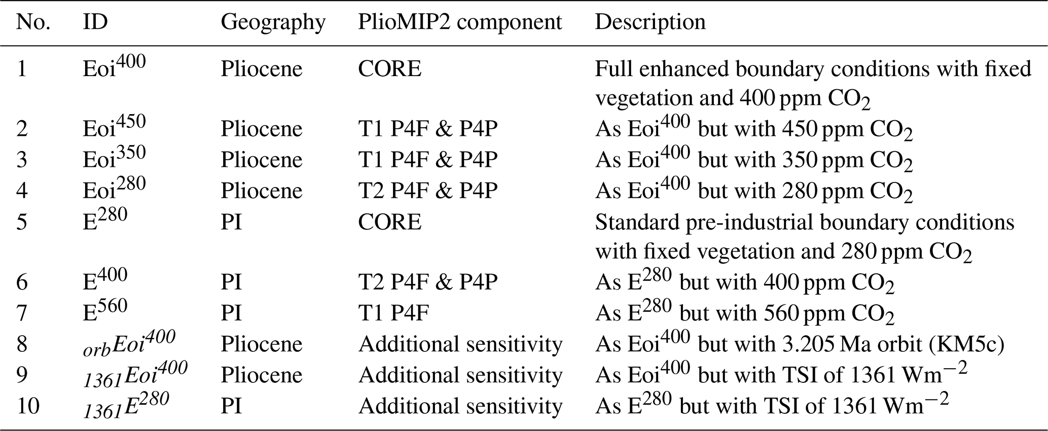
The following definitions are used: pre-industrial (PI), tier 1 (T1), tier 2 (T2), Pliocene for Future (P4F), Pliocene for Pliocene (P4P) and total solar irradiance (TSI).

2 Model description

We use the UK Meteorological Office (UKMO) HadCM3 coupled atmosphere–ocean general circulation model (AOGCM). A top-level description of the atmosphere and ocean models relevant to this palaeogeographic reconfiguration follows. Focus is given to the ocean model, as its external geometry is changed (the atmosphere model layers drape over the topography) and certain aspects impact upon the interpretation of model prediction. For a more comprehensive description of the fundamental model structure, see Pope et al. (2000) and Gordon et al. (2000). Subsequent corrections and improvements to the model, as well as a thorough evaluation against observational data, have been described in Valdes et al. (2017). The HadCM3 model used in this study is equivalent, in terms of model updates and modifications, to HadCM3B-M2.1a of Valdes et al. (2017). We keep with the name HadCM3 in reference to the UKMO (Pope et al., 2000; Gordon et al., 2000) but acknowledge the contribution made by the University of Bristol in keeping the HadCM3 model developed and updated.

The HadCM3 climate model is no longer state of the art but the model's runtime speed, relative ease of reconfiguration and prediction performance make it well suited for an ensemble of centennial-scale palaeoclimate simulations as is required here. HadCM3 can be integrated for many thousands of model years and reaches a satisfactory state of equilibrium with little drift in the surface climatology. However, there are a number of model weaknesses, compared to more contemporary models, and these will be discussed where relevant.

The HadCM3 model has been used extensively for studies of the Pliocene. The model was used within PlioMIP1 experiments 1 (atmosphere GCM) and 2 (atmosphere–ocean GCM) (Haywood et al., 2010, 2011; Bragg et al., 2012), and amongst others has been used to successfully investigate Panama Seaway closure (Lunt et al., 2008), El Niño–Southern Oscillation (ENSO) and teleconnections (Bonham et al., 2009), ice sheet reconstructions and orbital forcing (Dolan et al., 2011; Prescott et al., 2014), sea ice reconstructions (Howell et al., 2014), terrestrial and marine oxygen isotopes (Tindall and Haywood, 2015), and non-analogous aspects of Pliocene climate (Hill, 2015). In all cases, either a modern LSM and bathymetry was used or only specific regional palaeogeographical uncertainties were explored. This body of work therefore represents the first published record where HadCM3 has been reconfigured with a bespoke global Pliocene palaeogeography.

2.1 Atmosphere and land models

The atmosphere component of HadCM3 has 19 vertical hybrid sigma-pressure levels extending to 5 hPa. Horizontal resolution is 3.75^∘ longitude $\times \mathrm{2.5}{}^{\circ }$ latitude. The model has a time step of 30 min and is coupled to the ocean model (Sect. 2.2) at the end of every model day (Gordon et al., 2000). Atmospheric composition, other than CO₂ (described in Sect. 3.1 and 3.2), is equivalent to pre-industrial throughout (N₂O 270 ppb, CH₄ 760 ppb and no CFCs), consistent with both the PMIP2 protocol (the second phase of the Palaeoclimate Model Intercomparison Project; LSCE, 2007; Braconnot et al., 2007) and the previous Pliocene experiments conducted within PlioMIP1. Monthly distribution of ozone is derived from the Li and Shine (1995) climatology and ground-based troposphere measurements, corrected for the ozone hole (Johns et al., 2003). The radiative effects of background aerosol are represented by a simple parameterisation based on modern climatological conditions (Cusack et al., 1998).

The solar constant (total solar irradiance; hereafter TSI) is held fixed at 1365 Wm⁻² within all PlioMIP2 protocol experiments, a value consistent with the pre-industrial experiment within PMIP2 (LSCE, 2007; Braconnot et al., 2007) and CMIP5 (the fifth phase of the Coupled model Intercomparison Project; Taylor et al., 2012) as well as PlioMIP1. This value (derived in the 1990s) is used to remain consistent with previous work, and the authors acknowledge that spaceborne measurements indicate that TSI has decreased from 1371 in 1978 to 1362 Wm⁻² in 2013 (Kopp and Lean, 2011; Meftah et al., 2014). Indeed, the CMIP6 pre-industrial simulation (piControl) uses a value of 1361 Wm⁻² (Matthes et al., 2017). We therefore examine the impact of TSI choice within the context of both pre-industrial and Pliocene climates within Sect. 4.3.2. Recognising this source of uncertainty and the impact on climate anomalies (due to non-linear climate responses) is important, as the PlioMIP2 specification (Haywood et al., 2016, Sect. 2.3.1) leaves the choice of TSI to individual modelling groups, whose TSI may depend upon whether or not the group is a participant of CMIP6. The impact of TSI choice is minimised by the Pliocene community's use of climatological anomalies but should be considered when comparing model–model absolute indices (summer sea ice extent, AMOC strength, etc.).

The land surface scheme is MOSES 2.1 (Met Office Surface Exchange Scheme; Cox et al., 1999; Essery et al., 2003) which principally deals with the hydrology of the canopy to the subsurface and the surface energy balance (including subsurface thermodynamics). Within the scheme there are five plant functional types (PFTs: broadleaf and needleleaf trees, C₃ and C₄ grasses, and shrub) as well as soil (desert), lakes and ice. Each non-glaciated terrestrial grid cell can take fractional values of each surface type.

The HadCM3 PlioMIP1 study of Bragg et al. (2012) used an earlier version of MOSES (MOSES1) which treats each model grid cell as a homogeneous surface and uses effective parameters to calculate the grid cell's energy and moisture flux. However, MOSES2 introduced subgrid (tiled) heterogeneity and improved representation of surface and plant processes such that hydrological partitioning and energy balance are computed for each subgrid tile. A comparison of MOSES1 and MOSES2.1 can be found within Valdes et al. (2017). In this study, we incorporate a software update taken from the HadGEM2 climate model (Good et al., 2013) which corrects the temperature control of plant respiration (making the model MOSES2.1a in the nomenclature of Valdes et al., 2017).

Runoff is collected in drainage basins and delivered to associated coastal outflow points (on a $\mathrm{3.75}{}^{\circ }\times \mathrm{2.5}{}^{\circ }$ geographic grid). River transport is not modelled explicitly; instead, runoff is returned to the coastal outflow point in the uppermost ocean layer instantaneously at the atmosphere–ocean coupling step (Gordon et al., 2000). Internal drainage basins are present but the associated water loss is not explicitly modelled within the routing scheme. Instead, the loss of freshwater in the hydrological cycle is corrected using an artificial freshwater correction field applied to the uppermost surface of the ocean (Sect. 2.2). This freshwater closure also acts to correct the freshwater loss due to terrestrial snowfall accumulation.

2.2 Ocean and sea ice models

The ocean component is a rigid-lid model of the Bryan–Cox lineage (Bryan, 1969; Cox, 1984). In the vertical, there are 20 unevenly spaced levels, concentrated near the surface in order to improve representation of the surface mixed layer. The model uses z-coordinate vertical layers with bottom topography represented by “full” cells. This leads to a discontinuous representation of the bathymetry which has poorer fidelity at greater depths (where the thickness of levels is greatest). The ocean time step is 1 h, horizontal spatial resolution is $\mathrm{1.25}{}^{\circ }\times \mathrm{1.25}{}^{\circ }$, and the grid is aligned so that there are six ocean grid cells to each atmosphere grid cell ($\mathrm{3.75}{}^{\circ }\times \mathrm{2.5}{}^{\circ }$). To simplify coupling with the atmosphere model, the ocean model's coastline has a resolution of $\mathrm{3.75}{}^{\circ }\times \mathrm{2.5}{}^{\circ }$ at the uppermost level.

Within the modern boundary conditions, cells overlying important subgrid-scale channels, such as those along the Denmark Strait, the Iceland–Faroe and the Faroe–Shetland channels, and straits surrounding the Indonesian archipelago, are artificially deepened. Additionally, within the Greenland–Iceland–Scotland region, a convective adjustment scheme (Roether et al., 1994) is used to better represent downslope mixing that improves the representation of dense outflows that form the North Atlantic Deep Water (NADW). The scheme is not used for Antarctic Bottom Water (AABW). Water mass exchange through the Strait of Gibraltar, a channel that falls on the subgrid scale, is achieved with a diffusive pipe. This pipe provides transport of water properties through the 13 topmost layers of the ocean (∼1200 m) between the eastern Atlantic and the western Mediterranean. Other subgrid-scale channels, such as the Canadian Archipelago, Hudson Strait outflow and the Makassar Strait, remain spatially unresolved and therefore unrepresented. The latter has been shown to possess most of the Indonesian throughflow (Gordon and Fine, 1996) and so is compensated for within the model by a deepening of regional model bathymetry.

The freshwater budget of the ocean is balanced by fluxes from the river routing scheme and a freshwater correction applied to the uppermost ocean level. Within the pre-industrial (and associated CO₂ sensitivity experiments), the freshwater correction field is prescribed (time invariant). The correction field had been derived to provide closure of the model's modern hydrological cycle and consists of a uniform background component (0.01 mm d⁻¹) correcting internal drainage (Sect. 2.1) and an iceberg component (0.02 mm d⁻¹) whose geographic distribution is derived from modern observations (Gordon et al., 2000; Pardaens et al., 2003). Within the Pliocene experiments, we omit the time-invariant correction (including the iceberg component) and instead use an annual model-derived geographically invariant freshwater correction to reduce residual salinity drifts to zero. We justify this as we currently do not have a priori knowledge of the geographic distribution of iceberg melt consistent with the ice sheet distribution within the PlioMIP2 enhanced boundary conditions. In the Northern Hemisphere, we do not expect significant iceberg calving given the configuration of the Greenland Ice Sheet and the lack of marine terminating margins specified within the PRISM4 boundary conditions.

The rigid-lid streamfunction scheme imposes the need for bathymetry to be smoothed particularly in steep regions of the high latitudes and for islands to be specified as line integrals for the barotropic streamfunction. A major consequence of the latter is that the modern Bering Strait throughflow is not fully resolved as it sits between two model-defined continents between which the barotropic component of flow is poorly resolved. This impacts our interpretation of the Pliocene experiments (closed Bering Strait) with respect to the pre-industrial (open Bering Strait); this is discussed within Sect. 3.2.2. An advantage of the rigid-lid scheme on the other hand is that barotropic gravity waves are neglected, which facilitates the use of longer time steps.

The sea ice model is a simple thermodynamic scheme based upon Semtner (1976) with parameterisations for ice drift and concentration. To account for sea ice leads, upper boundaries of 0.995 and 0.980 are imposed on Arctic and Antarctic sea ice concentrations based upon the parameterisation of Hibler (1979). Ocean salinity is influenced by sea ice formation and melt by assuming a sea ice salinity of 0.6 psu (excess salt, in effect, is returned to the ocean). Sublimation is represented and acts to increase ocean salinity (salt blown into leads), whilst ocean-bound snowfall and precipitation reduce salinity. The effects of snow age and melt pond formation on surface albedo are represented with a linear parameterisation based upon surface temperature. Ice drifts only by the action of surface ocean current; hence, within the model surface, wind stress indirectly influences sea ice drift via its influence on the surface ocean current. Sea ice dynamics is represented by parameterisations based upon Bryan et al. (1975). Ice rheology is simply represented by preventing ice convergence above 4 m thickness. There is no representation for the interaction between floes.

3 Experiment design

Here, we describe the setup of the Pliocene and the pre-industrial experiments. The Pliocene experiments have CO₂ set to 280, 350, 400 and 450 ppm, each conducted with modern orbit as specified by the PlioMIP2 protocol (Haywood et al., 2016). These experiments are labelled the control Pliocene experiment Eoi⁴⁰⁰ (PlioMIP2 CORE), Eoi^350,450 (tier 1; P4F+P4P) and Eoi²⁸⁰ (tier 2; P4F). Here, we use a comma-separated list in the superscript to indicate 2 or more experiments. In all cases, the superscript indicates CO₂ (in ppm) and the o and i indicate the inclusion of the PRISM4 orography (including PRISM4 vegetation, soil and lakes) and ice sheets. The experiments based upon the pre-industrial geography are run with CO₂ values of 280, 400 and 560 ppm. These are identified as the control pre-industrial experiment E²⁸⁰ (CORE), E⁴⁰⁰ (tier 2; P4F) and E⁵⁶⁰ (tier 1; P4F).

We also explore two sets of non-protocol experiments to assess sensitivities to Pliocene orbital configuration and the TSI. The PlioMIP2 protocol (Haywood et al., 2016) specifies a modern orbital configuration for all Pliocene experiments. We investigate the validity of this orbit choice by rerunning Eoi⁴⁰⁰ with a 3.205 Ma orbital configuration representing the mid-Piacenzian warm period (mPWP) time slice of Haywood et al. (2013a) within experiment _orbEoi⁴⁰⁰. We also investigate the choice of total solar irradiance (Sect. 2.1) by rerunning the two control (CORE) experiments with a TSI of 1361 Wm⁻² within ₁₃₆₁E²⁸⁰ and ₁₃₆₁Eoi⁴⁰⁰.

In total, six Pliocene experiments were run: the CORE (Eoi⁴⁰⁰), two tier 1 (Eoi³⁵⁰ and Eoi⁴⁵⁰), one tier 2 (Eoi²⁸⁰), as well as an orbital (_orbEoi⁴⁰⁰) and TSI sensitivity experiment (₁₃₆₁Eoi⁴⁰⁰). These are accompanied by four pre-industrial-based experiments: the CORE (E²⁸⁰), a tier 1 (E⁵⁶⁰) and tier 2 (E⁴⁰⁰), as well as a TSI sensitivity experiment (₁₃₆₁E²⁸⁰). These 10 simulations are detailed within Table 1.

3.1 Pre-industrial and associated sensitivity experiments (E^280,400,560 and ₁₃₆₁E²⁸⁰)

The experiments with pre-industrial geography are 500-year continuations of a long integration (>2000 model years) pre-industrial experiment that had been initialised from the observed ocean state of Levitus and Boyer (1994). The experiment uses a topography and a bathymetry regridded and smoothed from ETOPO5 (National Geophysical Data Center, 1993), and vegetation and soil translated from the land cover of Wilson and Henderson-Sellers (1985). Within all experiments, the vegetation scheme is time invariant (fixed). River routing is derived by aggregating runoff in all terrestrial grid boxes within each runoff basin in a manner which is internally consistent with the model topography. All model boundary conditions were developed by the Met Office Hadley Centre (hereafter MOHC) and used within CMIP3/5. In accordance with the PlioMIP2 protocol (Haywood et al., 2016), levels of atmospheric CO₂ are set to 280, 400 and 560 ppm, giving the pre-industrial (E²⁸⁰) and two CO₂ sensitivity experiments (E⁴⁰⁰ and E⁵⁶⁰). A fourth pre-industrial-based experiment, ₁₃₆₁E²⁸⁰, is run to investigate the model sensitivity to the choice in TSI value (Sects. 2.1 and 4.3.2).

3.2 Pliocene (PlioMIP2 enhanced) and sensitivity experiments (Eoi^{280,350,400,450}, _orbEoi⁴⁰⁰ and ₁₃₆₁Eoi⁴⁰⁰)

3.2.1 Boundary condition preparation

For PlioMIP2, the boundary conditions for the modern-day and the “enhanced” variant of the Pliocene reconstruction are provided on regular 1^∘ grids held within NetCDF files (USGS, 2016; Haywood et al., 2016). For convenience, we shall refer to the PlioMIP2 enhanced boundary condition as PRISM4. The modern geography is provided to facilitate the anomaly method of boundary condition generation. The LSM is created by computing the anomaly of PRISM4 Pliocene minus PRISM4 modern (at 1^∘ resolution) and regridding using bilinear interpolating to the $\mathrm{3.75}{}^{\circ }\times \mathrm{2.5}{}^{\circ }$ model grid and then applying the anomaly to the model's pre-industrial LSM. This is so that the final reconstruction is consistent with both the original pre-industrial model setup and the PRISM4 LSM. Finally, a number of manual corrections were applied to the resulting $\mathrm{3.75}{}^{\circ }\times \mathrm{2.5}{}^{\circ }$ PRISM4 LSM to ensure that the underlying character of the PRISM4 reconstruction is represented as best as reasonably practicable at the model's resolution. For consistency with the pre-industrial boundary conditions developed by MOHC, we remove Svalbard and Novaya Zemlya, despite their subaerial extension within PRISM4. Similarly, we keep the Pliocene LSM in the Persian Gulf region the same as pre-industrial despite a withdrawal of the Persian Gulf within PRISM4. This choice was made as the Persian Gulf within the pre-industrial LSM is represented by an inland sea (due to inadequate spatial resolution) and so further changes would be difficult to interpret. At model resolution, the Pliocene Strait of Gibraltar is identical to the pre-industrial and so the diffusive pipe is incorporated.

The resulting PRISM4 LSM was used to constrain the generation of the Pliocene orography and bathymetry (which was generated using area-weighted regridding and then applied as an anomaly to the existing HadCM3 pre-industrial orography and bathymetry). River basins and outflow points were derived from the pre-industrial routing scheme (Sect. 3.1) but corrected in regions of LSM, topographical and ice–bedrock change using a model-resolution river routing model based on the D8 method (Tribe, 1992). This was then followed by manual correction in regions where model resolution fails to capture important orography, or where the regridded Pliocene orography is flat. The PRISM4 vegetation scheme (represented by BIOME4 biomes) was regridded by combining a BIOME4-to-MOSES2 lookup table with an area-weighted survey of underlying biomes. The vegetation scheme is then held fixed within each experiment. A similar area-weighted regridding was conducted for the lake field. We chose not to generate the lake field as an anomaly from the modern lake distribution, as land surface change since the pre-industrial would be imprinted on the model's lake distribution.

3.2.2 Barotropic streamfunction island configuration

Rigid-lid Bryan–Cox-type models, such as the ocean of HadCM3, require islands (and by extension, continents) to be identified so that a net non-zero barotropic flow (depth independent) can be achieved around the line integral (streamfunction non-zero). The default pre-industrial configuration of the model has six islands defined and is shown within Fig. 1. For consistency, aforementioned (Sect. 3.2.1) manual corrections to both LSM and bathymetry have allowed islands to be specified that are consistent with the E²⁸⁰ experiment but also reflect the key palaeogeographic changes presented by the PRISM4 palaeogeography. In particular, western Iceland and East Greenland land cells were adjusted to ensure that Iceland could be defined as a streamfunction island (Fig. 1), and hence we could fully represent the East Greenland Current. The island to the west of the Antarctic Peninsula body lies outside the island definition of the main Antarctic continent and therefore the circulation between the two is not fully resolved (only the baroclinic flow is resolved fully). Figure 1 compares the pre-industrial and PRISM4 Pliocene HadCM3 island specification. It can be seen that the six islands in the pre-industrial configuration have been increased to eight islands in the Pliocene.

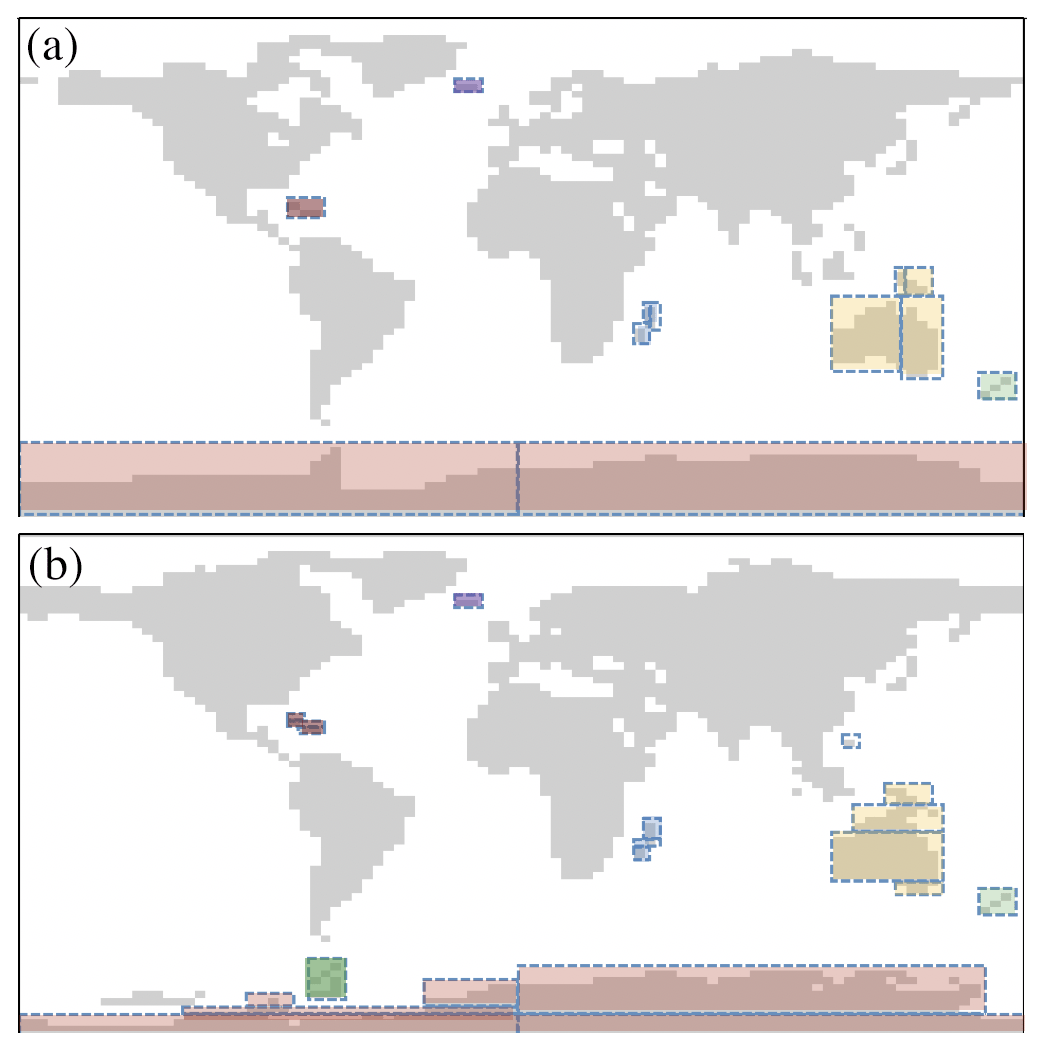
Figure 1 LSM and barotropic streamfunction island configuration for the (a) pre-industrial and (b) Pliocene.

It is noted that within the pre-industrial HadCM3 model setup the Bering Strait barotropic component of throughflow is unresolved and both the Makassar Strait and the Canadian Archipelago are spatially unresolved (Sect. 2.2). This poses a conceptual problem in the interpretation of the Pliocene experiments with respect to the pre-industrial, as the PRISM4 Pliocene geography has these throughflow regions closed. Therefore, our simulations do not resolve the full climatic response of these regional palaeogeographic changes. A pre-industrial experiment with a fully resolved Bering Strait and Canadian Archipelago would partially address these problems but would then force a divergence away from the previous HadCM3 descriptions and evaluations, as well as from past and current CMIP/PMIP and PlioMIP1 model implementations. These problems are likely to arise in all rigid-lid streamfunction ocean models that have insufficient spatial resolution to fully resolve these gateways and inherently cannot resolve line integrals around bounding land masses. Ocean models that have explicit or implicit free-surface schemes with sufficiently high horizontal spatial resolution may reduce these issues.

3.3 Pliocene model initialisation and spin-up

Model spin-up is conducted in a series of stages in which the model and boundary conditions are increased in complexity. These stages are as follows:

1. The atmosphere model (AGCM) was initialised in a 50-year run with PRISM4 LSM, basic surface scheme (lakes, ice, shrubs and orography), pre-industrial CO₂ (280 ppm), as well as zonal hemispheric-symmetric monthly sea surface temperature (SST) and sea ice distribution derived from the initial 2500 model year pre-industrial HadCM3 simulation from Sect. 3.1. Model failures at this stage allow for the identification of steep topography that requires regional smoothing.

2. The ocean model is added (without barotropic physics) and the resulting AOGCM run is continued for 100 years with Pliocene bathymetry and river scheme (year 50 within Fig. 2).

3. Barotropic physics is incorporated (without specifying islands) and the simulation is continued for 200 years. Regional bathymetric smoothing was applied in regions which caused model failure (Fig. 2 stage a).

4. The island configuration (Sect. 3.2.2, Fig. 1) is then derived using an iterative series of sensitivity tests in which each island configuration is refined. Once complete, the set of island line integrals is incorporated into the model configuration. At this stage, we have an AOGCM incorporating full barotropic physics (Fig. 2 stage b).

5. CO₂ is increased from 280 ppm at 1 % yr⁻¹ until 400 ppm is attained. CO₂ is then held fixed.

6. At model year 950, a problem with ancillary file generation had been resolved allowing the vegetation boundary condition to be incorporated into the model. Additionally, a regional modification was made to the bathymetry and streamfunction island configuration to the west of the Antarctic Peninsula to resolve a persistent numerical mode within the barotropic solver in this region (Fig. 2 stage c). The final island configuration is shown within Fig. 1.

7. The AOGCM model was then set to continue to the year 2000.

8. At the year 2000, five additional experiments are spun off that run alongside Eoi⁴⁰⁰ (Table 1). These are Eoi${}^{\mathrm{280},\mathrm{350},\mathrm{450}}$, _orbEoi⁴⁰⁰ and ₁₃₆₁Eoi⁴⁰⁰. All six experiments are run to the year 2400.

9. The models are then run for the final 100 years configured with full climatological output.

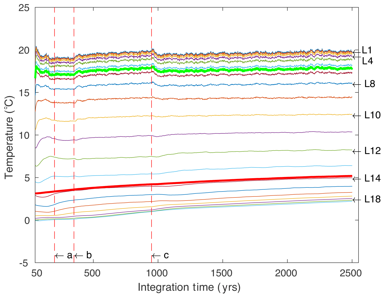
Figure 2 Time evolution of the globally integrated temperature for the ocean layers within the Eoi⁴⁰⁰ experiment. Whole ocean volume is indicated by the thick red line and the top 200 m are indicated by the thick green line. Vertical lines indicate key spin-up stages: (a) adding the barotropic physics to the ocean model, (b) incorporation of barotropic streamfunction islands into the barotropic solver and (c) correction to the barotropic streamfunction island in the southern high latitudes and incorporation of full PRISM4 vegetation boundary conditions into the model. The midpoints to the ocean layers are 5 m (L1), 15 m (L2), 15 m (L3), 35 m (L4), 48 m (L5), 67 m (L6), 96 m (L7), 139 m (L8), 204 m (L9), 301 m (L10), 447 m (L11), 666 m (L12), 996 m (L13), 1501 m (L14), 2116 m (L15), 2731 m (L16), 3347 m (L17), 3962 m (L18), 4577 m (L19) and 5195 m (L20).

3.4 Equilibrium state

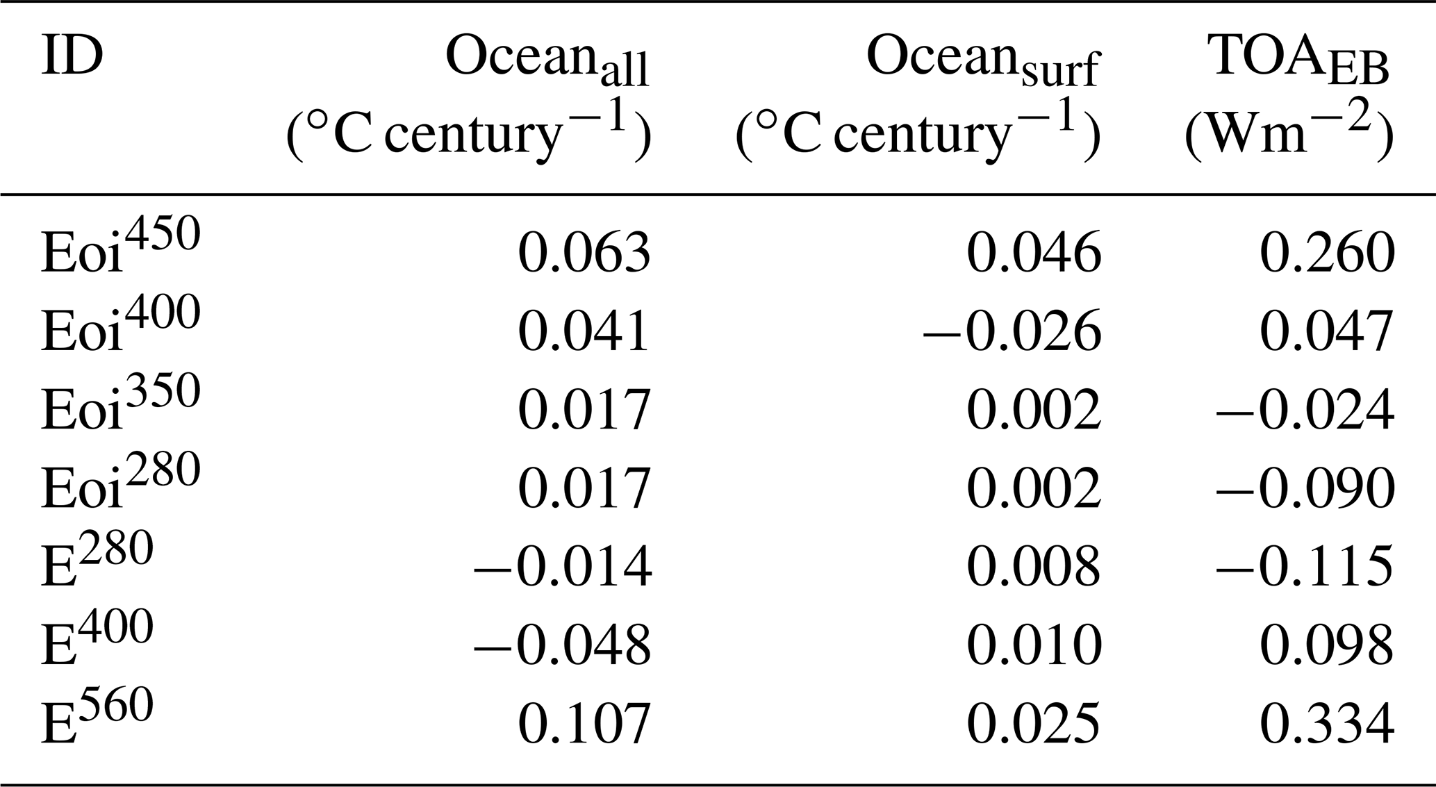
By model years 2400 to 2500, the Pliocene control experiment (Eoi⁴⁰⁰) has achieved a quasi-steady-state equilibrium in which the globally integrated net top-of-the-atmosphere (TOA) radiative imbalance is 0.047 Wm⁻², surface (1.5 m) air temperature trend is 0.08 ^∘C century⁻¹ and ocean potential temperature trends within the upper 200 m and globally integrated are −0.026 and 0.041 ^∘C century⁻¹. The corresponding values for the pre-industrial control experiment (E²⁸⁰) are −0.115 Wm⁻², 0.052, 0.008 and −0.014 ^∘C century⁻¹, respectively. High-CO₂ experiments, Eoi⁴⁵⁰ and E⁵⁶⁰ present the largest, yet modest, departures from equilibrium and are characterised by TOA imbalance >0.2 Wm⁻². Positive TOA imbalance is indicative of a warming of the Earth system, the small heat capacity of the atmosphere means that residual energy is predominantly taken up by the ocean, which is reflected in the volume-integrated ocean temperature evolution. Warming of the deep ocean is primarily occurring at depths deeper than 2000 m in the Pacific basin. The Indian and Antarctic oceans are the most equilibrated, particularly at intermediate depths and deeper. Table 2 summarises the equilibrium states of the seven PlioMIP2 experiments and Fig. 2 presents the time evolution of ocean potential temperature of the Pliocene control experiment (Eoi⁴⁰⁰). All experiments are deemed to be in a satisfactory state of equilibrium, although the high TOA imbalance simulations Eoi⁴⁵⁰ and E⁵⁶⁰ have above-average warming within the deep ocean.

Table 2 Summary of equilibrium state metrics for the seven PlioMIP2 protocol experiments. Globally integrated (Ocean_all) and surface ocean (top 200 m; Ocean_surf) climatological trends and top-of-the-atmosphere energy balance (TOA_EB) are derived from the last 100 model years.

4 Results

We base our analysis on climatological averages from the final 50 years of each simulation. The final 50 years of output are used to remain consistent with the HadCM3 PlioMIP1 submission (Exp. 2 of Bragg et al., 2012). The PlioMIP2 protocol (Haywood et al., 2016) does not state a standardised time length for climatological means although the PlioMIP2 website (USGS, 2018) does request 100 years of monthly climatology. We therefore make the 50-year climatological average and 100 years of monthly climatology available on the PlioMIP2 data repository.

In order to keep discussion clear and concise, we principally compare the two PlioMIP2 CORE experiments, which we refer to as the control experiments (Eoi⁴⁰⁰ and E²⁸⁰). Whilst there is uncertainty in mid-Piacenzian (MIS KM5c) CO₂ levels, 400 ppm represents the middle of the anticipated CO₂ range derived from marine- and terrestrial-based reconstructions (Haywood et al., 2016, and references therein). We therefore consider Eoi⁴⁰⁰ as our “best estimate” simulation. In addition, when referring to climate forcing, we use the term “palaeogeography” to encompass the combined change in topography, land surface (vegetation, lakes, soils, ice sheets), LSM and bathymetry which we diagnose from the anomaly Eoi²⁸⁰ minus E²⁸⁰.

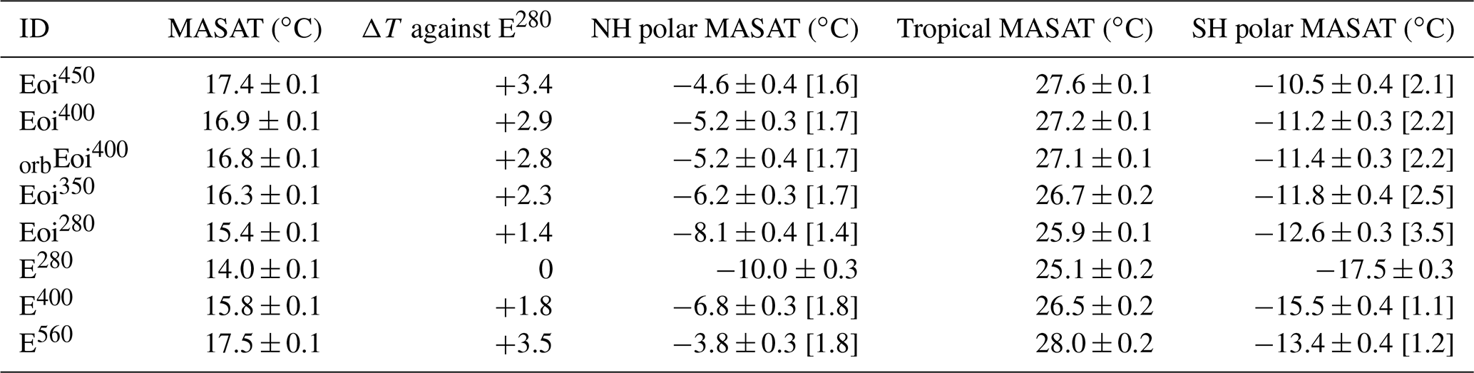
Table 3 Global mean annual surface air temperature (MASAT) and the mean annual surface air temperatures of the polar (poleward of 60^∘) and tropical (equatorward of 30^∘) regions. The polar amplification factor is shown in square brackets and is defined as the ratio in the anomalies (against E²⁸⁰) between the polar warming and the global mean warming.

4.1 State of the atmosphere and Earth surface climatology

4.1.1 Surface air temperature and climate sensitivity

Modelled mean annual 1.5 m surface air temperatures (hereafter MASAT) are detailed within Table 3 and corresponding Pliocene anomalies are shown within Fig. 3. Relative to the pre-industrial control (E²⁸⁰) temperatures are generally warmer within the Pliocene experiments. Very high differences in MASAT of up to 31.3 ^∘C are reached over regions of Greenland and Antarctica, where the elevation of Pliocene ice sheets has been changed with respect to the present. Typically, warming is greatest over land, although in ocean regions at or near Antarctic LSM change (pre-industrial grounded ice to Pliocene ocean) warming is significant. This pattern of warming is similar to results derived with HadCM3 within PlioMIP1 under PRISM3 boundary conditions (Exp. 2 of Bragg et al., 2012).

Figure 3 Pliocene annual mean surface air temperature anomalies against E²⁸⁰. (a) Eoi⁴⁵⁰–E²⁸⁰, (b) Eoi⁴⁰⁰–E²⁸⁰, (c) Eoi³⁵⁰–E²⁸⁰ and (d) Eoi²⁸⁰–E²⁸⁰. Stippling indicates regions in which results are not statistically significant at a 95 % confidence criterion (independent two-sample Student's t test).

The Pliocene cooling in the Barents Sea is statistically significant and persistent through the model integration (Fig. 3). It coincides with an increase in Pliocene winter and spring sea ice concentration driven by palaeogeographic terrestrial winter cooling in the circum-Arctic (Pliocene subaerial Barents and Baltic Sea). This cooling is potentially driven by the partial suppression of northward heat transport (in the Norwegian Current) by the subaerial extension of Ireland and Scotland within the model.

The Eoi⁴⁰⁰–E²⁸⁰ MASAT anomaly of 2.9 ^∘C (Table 3) is lower than the 3.3 ^∘C of HadCM3 within PlioMIP1 (Bragg et al., 2012) and lies within the PlioMIP1 model ensemble range of 1.84–3.60 ^∘C (Haywood et al., 2013b). The MASAT anomaly also lies between the PlioMIP2 studies of Kamae et al. (2016) (2.4 ^∘C) and Chandan and Peltier (2017) (3.8 ^∘C), although note that this comparison is not exhaustive as PlioMIP2 is incomplete at the time of press. Table 3 also presents MASAT data for the equatorial (between 30^∘ S and 30^∘ N) and polar regions (latitudes greater than 60^∘). The resulting polar amplification factors for the Pliocene control (Eoi⁴⁰⁰) relative to the pre-industrial control (E²⁸⁰) are 1.7 for the Northern Hemisphere and 2.2 for the Southern Hemisphere.

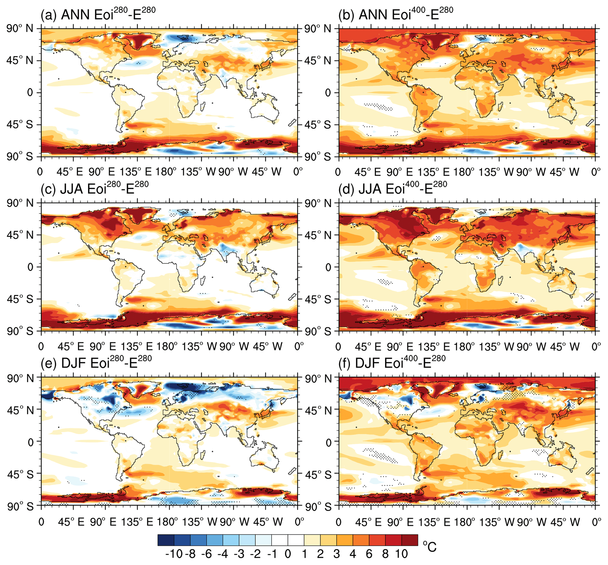
Figure 4 Mean annual and seasonal Pliocene temperature anomalies against E²⁸⁰. (a) Annual Eoi²⁸⁰–E²⁸⁰, (b) annual Eoi⁴⁰⁰–E²⁸⁰, (c) June–July–August (JJA) Eoi²⁸⁰–E²⁸⁰, (d) JJA Eoi⁴⁰⁰–E²⁸⁰, (e) December–January–February (DJF) Eoi²⁸⁰–E²⁸⁰ and (f) DJF Eoi⁴⁰⁰–E²⁸⁰. Stippling indicates regions in which results are not statistically significant at a 95 % confidence criterion.

Figure 4 shows the annual and seasonal temperature anomalies for Eoi²⁸⁰ and Eoi⁴⁰⁰ (against E²⁸⁰). Terrestrial regions that are exposed only within the Pliocene, such as the Hudson Bay and the Baltic Sea regions, are up to 10 ^∘C warmer (colder) during the summer (winter) seasons, due to land–ocean heat capacity contrast. It is unclear how much of this seasonal temperature response in the Baltic Sea region (exposed during the Pliocene) is a driver of persistent cooling within the Barents Sea region.

From the results in Table 3, it is possible to diagnose the factors that contribute to Pliocene warming relative to the pre-industrial (E²⁸⁰). Considering the Pliocene control experiment (Eoi⁴⁰⁰), we find that the change in palaeogeography (Eoi²⁸⁰–E²⁸⁰) accounts for a temperature change of 1.4 ^∘C, whilst the increase in CO₂ (Eoi⁴⁰⁰–Eoi²⁸⁰) accounts for a further 1.5 ^∘C of warming. Considering uncertainty in Pliocene CO₂ level, we find temperature changes of 0.9 and 2.0 ^∘C for Eoi³⁵⁰–Eoi²⁸⁰ and Eoi⁴⁵⁰–Eoi²⁸⁰, respectively. The PlioMIP2 experimental design provides a second pathway to examine Pliocene palaeogeographical and CO₂ forcing (e.g. Eoi⁴⁰⁰–E⁴⁰⁰ and E⁴⁰⁰–E²⁸⁰). Within this pathway, the Pliocene geography (Eoi⁴⁰⁰–E⁴⁰⁰) accounts for 1.1 ^∘C of warming and the increase in CO₂ (E⁴⁰⁰–E²⁸⁰) accounts for 1.8 ^∘C of temperature increase. These differences highlight that there are non-linearities within the climate system's response to changes in boundary condition.

The climate system's sensitivity to a doubling of CO₂ (climate sensitivity; CS) is 3.5 ^∘C for the pre-industrial (derived from E⁵⁶⁰ and E²⁸⁰) and 2.9 ^∘C for the Pliocene (derived from Eoi⁴⁰⁰ and Eoi²⁸⁰ and scaled by 1.94 ($=\log (\mathrm{560}/\mathrm{280})/\log (\mathrm{400}/\mathrm{280})$). The pre-industrial CS is consistent with the 3.3 ^∘C for HadCM3 within CMIP3 (Randall et al., 2007). The Pliocene CS is similar to the 3.1 ^∘C for HadCM3 and lies at the lower end of the 2.7–4.1 ^∘C ensemble range of PlioMIP1 experiment 2 (Haywood et al., 2013b). When we approximate Earth system sensitivity (ESS) using Eoi⁴⁰⁰ and E²⁸⁰ (with ESS $=\mathrm{1.94}x\mathrm{\Delta }{T}_{{\text{Eoi}}^{\mathrm{400}}{\text{–E}}^{\mathrm{280}}}$), we obtain ∼5.6 ^∘C. Subsequently the ESS ∕ CS ratio is ∼1.9, which lies at the higher end of the 1.1–2.0 range of the PlioMIP1 ensemble (Haywood et al., 2013b) in which HadCM3 had a ratio of 2.0. It must be noted, however, that such a comparison of CS and ESS is only meaningful when one assumes that the PlioMIP2 enhanced boundary condition approximates the equilibrated Earth system under a contemporary doubling of CO₂, which is a reasonable position since the changes in non-glacial elements of the PRISM4 retrodicted palaeogeography are relatively small.

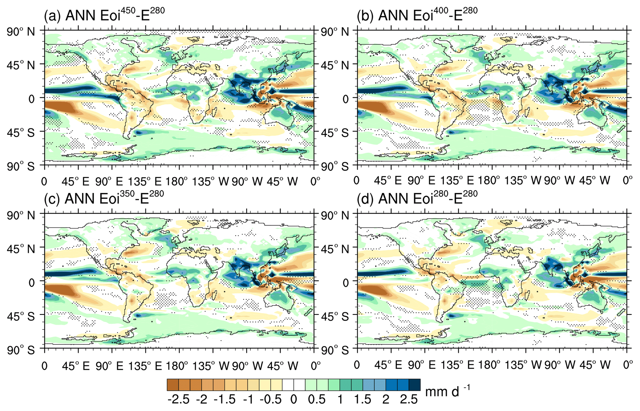
Figure 5 Pliocene mean annual precipitation anomalies against E²⁸⁰. (a) Eoi⁴⁵⁰–E²⁸⁰, (b) Eoi⁴⁰⁰–E²⁸⁰, (c) Eoi³⁵⁰–E²⁸⁰ and (d) Eoi²⁸⁰–E²⁸⁰. Stippling indicates regions in which results are not statistically significant at a 95 % confidence criterion.

4.1.2 Precipitation

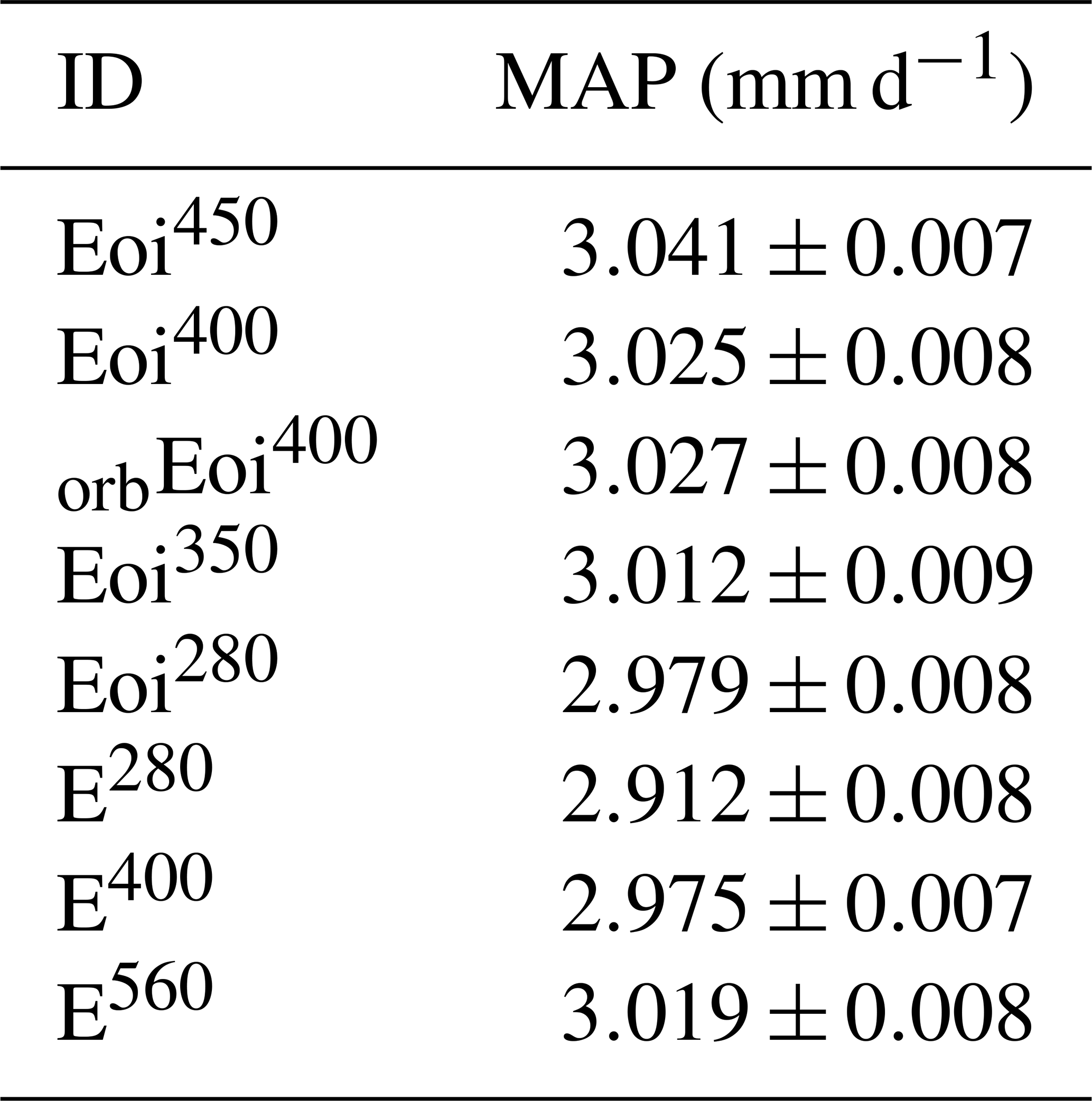
The globally integrated mean annual precipitation (MAP; Table 4) is influenced by both Pliocene geography and CO₂ changes. Pliocene geography acts to increase globally integrated MAP, although this appears sensitive to the background CO₂ level (e.g. Pliocene geography increases MAP by 0.07 and 0.05 mm d⁻¹ at 280 and 400 ppm, respectively). The Eoi⁴⁰⁰–E²⁸⁰ MAP anomaly of 0.11 mm d⁻¹ (Table 4) compares with the 0.17 mm d⁻¹ from HadCM3 within PlioMIP1 (Bragg et al., 2012) and sits at the lower end of the ∼0.09–0.18 mm d⁻¹ range of the PlioMIP1 model ensemble (Haywood et al., 2013b).

Table 4 Globally integrated mean annual precipitation (MAP).

The geographical distribution of MAP change can be seen within Fig. 5. Northern Hemisphere land masses generally see increased precipitation within the Pliocene, although this effect is minimal in the continental interiors. In the Southern Hemisphere, much of South America and south Africa receive less precipitation, whilst Australia and northern Greenland see an increase in precipitation during the Pliocene. Increasing Pliocene CO₂ generally intensifies the precipitation anomaly, which is most apparent in the tropics. Regions that receive little precipitation within E²⁸⁰; e.g. north Africa and the East Antarctic Ice Sheet have little (<0.1 mm d⁻¹) change in precipitation under increasing Pliocene CO₂.

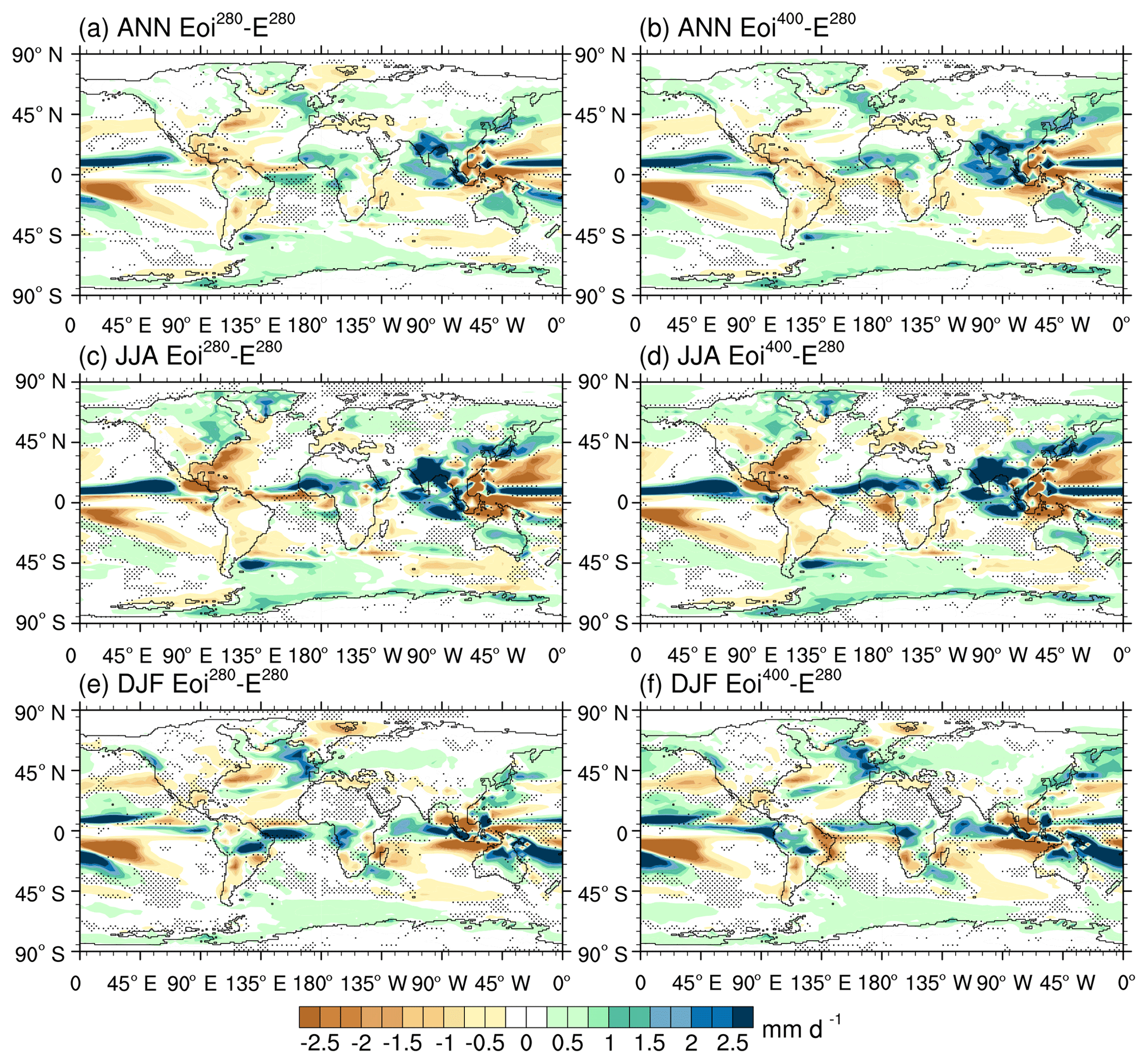
Figure 6 Mean annual and seasonal Pliocene precipitation anomalies. (a) Annual Eoi²⁸⁰–E²⁸⁰, (b) annual Eoi⁴⁰⁰–E²⁸⁰, (c) JJA Eoi²⁸⁰–E²⁸⁰, (d) JJA Eoi⁴⁰⁰–E²⁸⁰, (e) DJF Eoi²⁸⁰–E²⁸⁰ and (f) DJF Eoi⁴⁰⁰–E²⁸⁰. Stippling indicates regions in which results are not statistically significant at a 95 % confidence criterion.

Table 5 Climatological zonal mean core latitude of the subtropical jet (StJ) for E²⁸⁰, Eoi²⁸⁰ and Eoi⁴⁰⁰ experiments during December–January–February (DJF) and June–July–August (JJA) seasons. Note that only the StJ is reported as it is more stable and persistent than the polar jet.

Seasonal plots of precipitation change between the Pliocene (Eoi⁴⁰⁰) and the pre-industrial (E²⁸⁰) control experiments are shown in Fig. 6. During the Pliocene, we see wetter summers over much of North America and northern Europe. Regions experiencing reduced precipitation in western North America as well as central and western Europe are a consequence of weakened westerlies (not shown). As can be seen within Fig. 6c–f, the Pliocene geography and land surface change drive an intensification of precipitation associated with the Intertropical Convergence Zone (ITCZ), although changes in seasonal latitudinal distribution are not evident. The South Pacific Convergence Zone, extending from the western Pacific warm pool (WPWP) southeastward to the south central Pacific, extends ∼15^∘ further east in E²⁸⁰ than Eoi⁴⁰⁰ and Eoi²⁸⁰.

4.1.3 Planetary-scale atmospheric circulation

The time-averaged zonal mean meridional mass transport streamfunction for the atmosphere is shown within Fig. 7. Clearly distinguished are the Hadley, the Ferrel and the polar cells. Taking the maximum of the meridional streamfunction as a measure of the Hadley cell strength, we find that the Pliocene geography acts to weaken (intensify) the Hadley cell within the Northern (Southern) Hemisphere. Looking at E²⁸⁰, we find the northern cell is stronger (+10.8 %) than the southern cell, which is in contradiction with observational and reanalysis data (Stachnik and Schumacher, 2011) that consistently show the southern cell being stronger than the northern cell. With increasing Pliocene CO₂, the southern cell intensifies and becomes stronger than the north (+19 % in Eoi²⁸⁰ and +42 % in Eoi⁴⁰⁰). This intensification (weakening) of the Hadley cell under changed land surface and geography should be driven by steepening (shallowing) of the tropical meridional temperature gradients in the tropics south (north) of the ITCZ. Coincident with the change in land surface and geography (Eoi²⁸⁰–E²⁸⁰) is a weakening of the combined annual mean overturning within the two Hadley cells (191 and 180×10⁹ kg s⁻¹ for E²⁸⁰ and Eoi²⁸⁰, respectively).

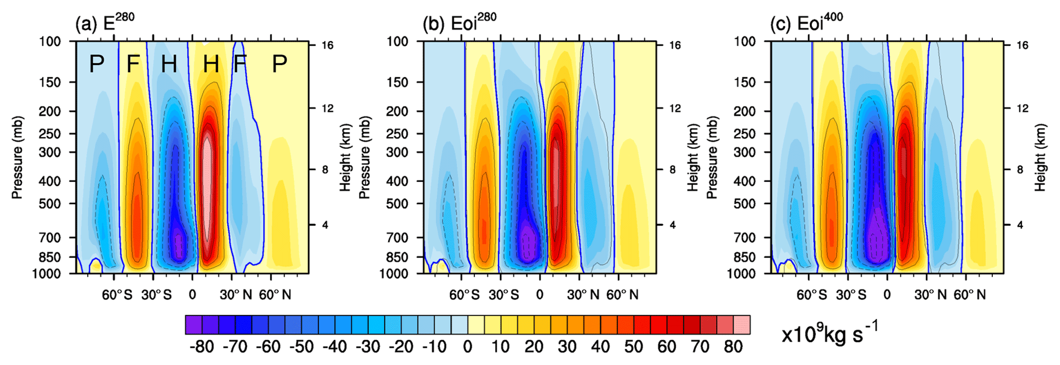
Figure 7 Mean annual zonally averaged meridional mass transport streamfunction for (a) E²⁸⁰, (b) Eoi²⁸⁰ and (c) Eoi⁴⁰⁰. The contour lines are from E²⁸⁰ and are shown for intervals of 2×10¹⁰ kg s⁻¹ with dashed lines indicating anticlockwise (looking westward) circulation (ascending air moves southward). The solid blue contour indicates zero meridional streamfunction indicative of the boundary of circulation cells. The Hadley (H), Ferrel (F) and the polar (P) cells are indicated within panel (a).

Table 6 Global mean annual sea surface temperature (MASST) and various metrics for the spatial extent of the equatorial warm pool regions.

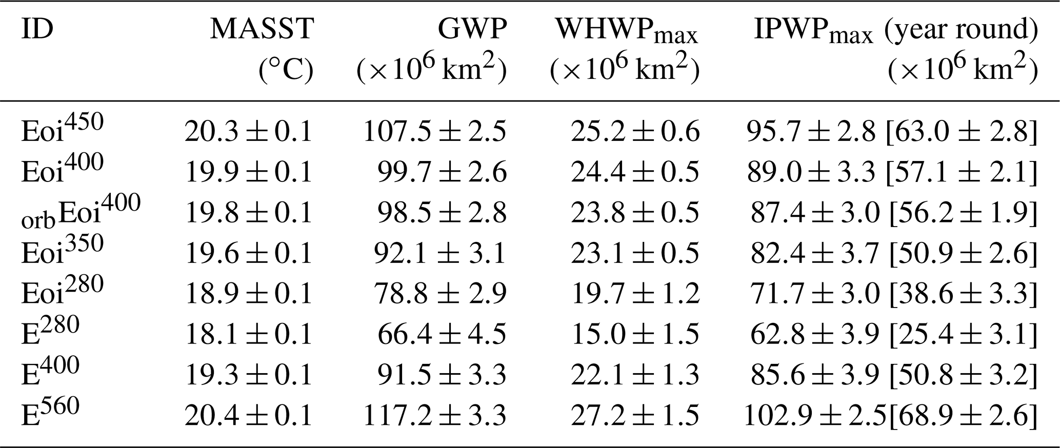
The global warm pool (GWP) area defined using MASST and a 28 ^∘C criterion. Western Hemisphere warm pool (WHWP; 130–45^∘ W) and Indo-Pacific warm pool (IPWP; 30^∘ E–60^∘ W) are defined as the max monthly mean area that is >28 ^∘C. For IPWP_max, the number in parentheses is the area that is >28 ^∘C year round.

The wintertime subtropical jet (StJ; also known as the midlatitude jet) and polar jet (PJ) are shown within Fig. 8. We characterise the mean spatial envelope of the jet path by deriving, from 50 years of daily data, the days per season in which the mean mass-weighted flow speed integrated over 400–100 hPa (∼7–16 km) exceeds 30 ms⁻¹. For both E²⁸⁰ (Fig. 8a–d) and E⁴⁰⁰ (not shown), we obtain a seasonal jet stream configuration which is consistent with the ERA-40 and derived results of Archer and Caldeira (2008). The PJ and the StJ streams can be difficult to differentiate as the former is latitudinally irregular, so following Koch et al. (2006) we use normalised wind shear as a height differentiator. The StJ stream path is more persistent and stable and so is characterised by the mean latitude of the StJ core which is shown within Table 5. The change in geography (Eoi²⁸⁰–E²⁸⁰) drives a poleward shift of the mean StJ latitude of ∼1.6^∘ in the Northern Hemisphere (both seasons) and 2.2^∘ in the Southern Hemisphere summer. The response to Pliocene CO₂ (Eoi⁴⁰⁰–Eoi²⁸⁰) increase is weaker with a 0.8^∘ poleward shift of the mean StJ latitude in the Northern Hemisphere (both seasons). The Southern Hemisphere mean StJ appears only weakly poleward shifting in response to Pliocene CO₂ increase. Regionally, jet behaviour deviates from the global mean view. Within the North Atlantic, the PJ moves equatorward in response to the change in palaeogeography (Eoi²⁸⁰–E²⁸⁰) moving the jet stream mean path from northern to southern Europe (Fig. 8b vs. 8f). Synoptic storms grow and propagate along jet stream axes, and so this equatorward shift in the PJ likely contributes to the increase in rainfall seen in southern Europe during Pliocene wintertime (Fig. 6e vs. 6f).

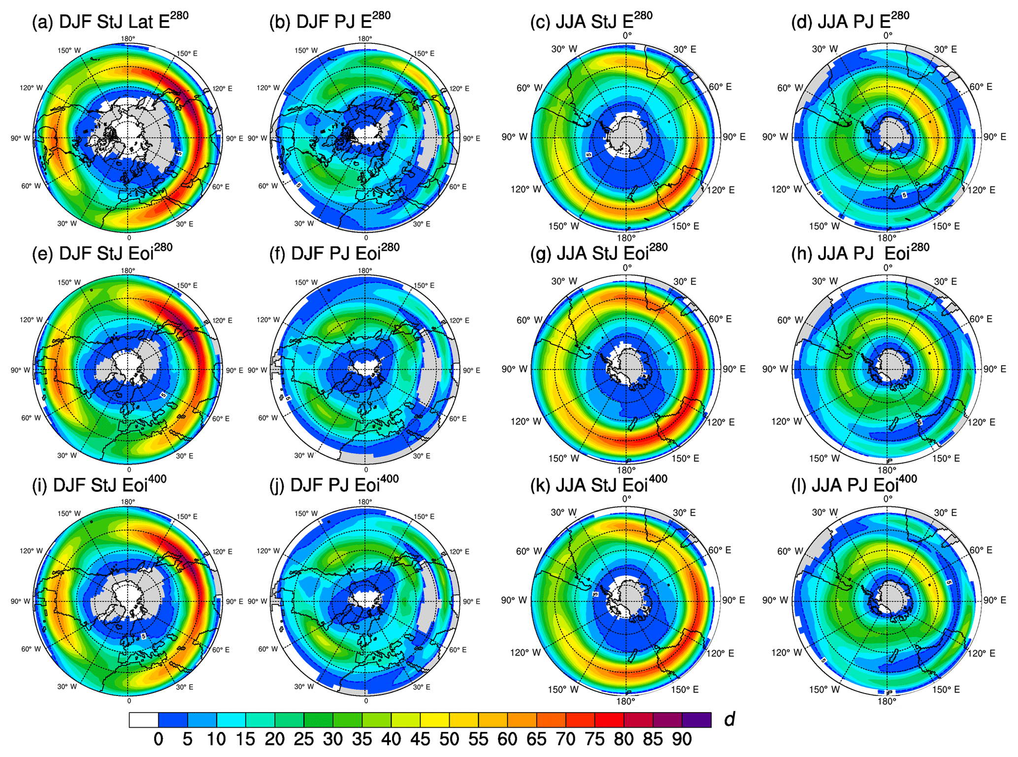
Figure 8 Seasonal (DJF and JJA) distribution of the StJ and PJ streams for (a–d) E²⁸⁰, (e–h) Eoi²⁸⁰ and (i–l) Eoi⁴⁰⁰. Colour scale indicates the mean number of days within a season in which wind speed is >30 ms⁻¹ over 400–100 hPa. Note that the wind-shear PJ classification identifies a jet downstream of the Himalayas.

4.2 State of the ocean climatology

4.2.1 Sea surface temperature and warm pools

Modelled mean annual SSTs (MASSTs) are detailed within Table 6 and Pliocene anomalies are shown within Fig. 9. We see a 0.8 ^∘C warming due to the change in palaeogeography (Eoi²⁸⁰–E²⁸⁰) and a further 1.0 ^∘C of warming due to the change in Pliocene CO₂ (Eoi⁴⁰⁰–Eoi²⁸⁰). With increasing levels of CO₂, regional patterns of MASST change due to palaeogeography are overprinted by CO₂-induced warming which is most evident in the midlatitudes. The greatest warming occurs within the North Atlantic subpolar gyre where Eoi⁴⁰⁰–E²⁸⁰ reaches 9.3 ^∘C. In the vicinity of the modern Gulf Stream and North Atlantic Drift, we find a cooling during DJF and MAM seasons of up to −4.9 ^∘C within Eoi²⁸⁰–E²⁸⁰ (not shown). Investigation of surface ocean velocity vectors (not shown) suggests an intensification of the North Atlantic wind-driven subpolar gyre which appears to disrupt western intensification and the path of the Gulf Stream. The westerlies in the region appear to intercept the remnant Gulf Stream and divert it from a northeasterly to a more eastward path. This is seen as the warm tongue south of the extant Gulf Stream (Fig. 9). A similar expression of MASST within the North Atlantic was seen by Chandler et al. (2013), and characteristic signatures may be present within other PlioMIP1 experiments (e.g. Fig. 1 of Dowsett et al., 2013). A persistent cooling is also found within the Barents Sea region coincident with the surface air temperature anomalies discussed within Sect. 4.1.1.

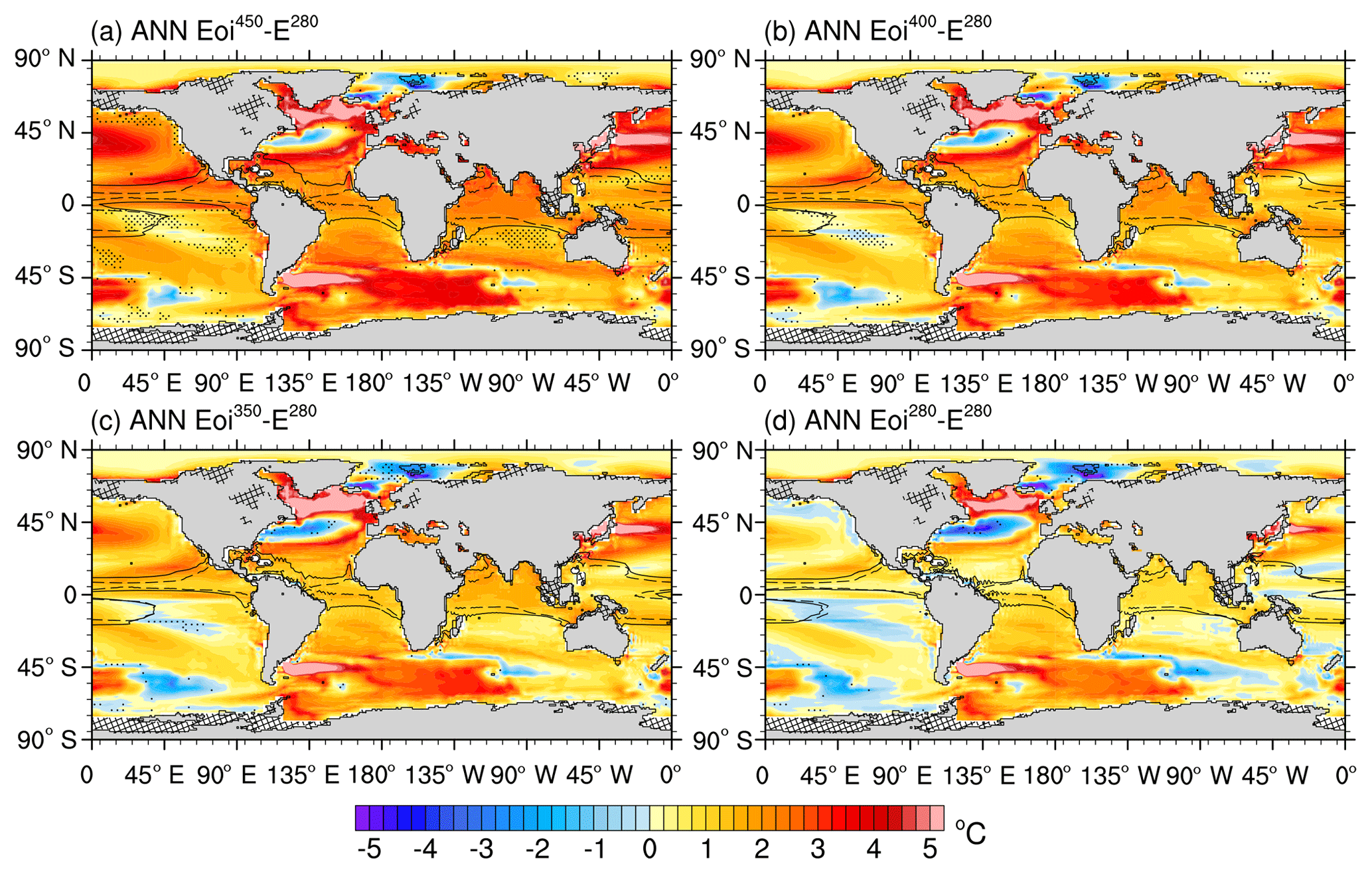
Figure 9 Pliocene MASST anomalies against E²⁸⁰. (a) Eoi⁴⁵⁰–E²⁸⁰, (b) Eoi⁴⁰⁰–E²⁸⁰, (c) Eoi³⁵⁰–E²⁸⁰ and (d) Eoi²⁸⁰–E²⁸⁰. Dotted contour lines indicate E²⁸⁰ 28 ^∘C warm pool, whilst the solid contour indicates the Pliocene 28 ^∘C warm pool. Cross hatching indicates regions in which either modern or Pliocene experiments have contrasting land surface. Stippling indicates regions in which there is no statistical difference at a 95 % confidence criterion.

Table 7 Characteristics of the Atlantic and Pacific meridional overturning circulations (AMOC and PMOC).

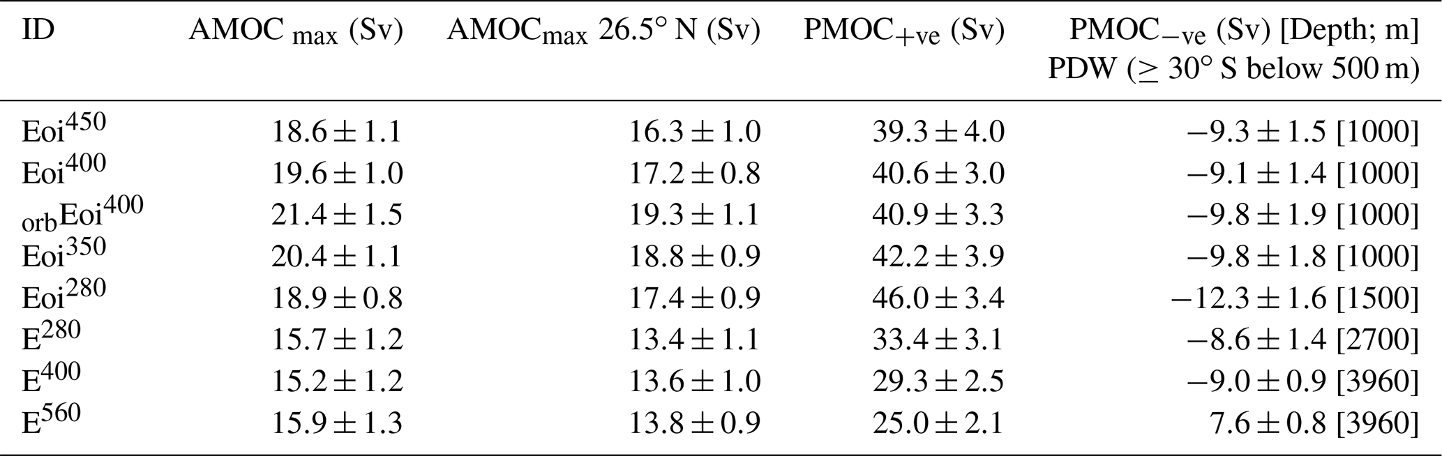
AMOC_max is the maximum AMOC. PMOC_+ve reflects the subtropical gyre circulation, whilst PMOC_−ve reflects the Pacific Deep Water (PDW) and North Pacific Deep Water (NPDW).

Table 6 also details the size of the global and component equatorial warm pools within the pre-industrial and Pliocene experiments. We see an expansion of the globally integrated warm pool with the change in palaeogeography (Eoi²⁸⁰–E²⁸⁰). This is evident in both the Western Hemisphere warm pool (WHWP) and Indo-Pacific warm pool (IPWP) regions. As expected, increased CO₂ drives warm pool expansion under both modern and Pliocene geographic conditions.

4.2.2 Sea ice

A complex picture emerges in the sensitivity of seasonal sea ice distribution to geographic and CO₂ changes as shown within Fig. 10. Within the Northern Hemisphere winter, the palaeogeography changes drive an equatorward expansion of sea ice in the Greenland Sea region. Increasing CO₂ from 280 to 400 ppm counteracts some of this expansion. In the Southern Hemisphere, the palaeogeographical changes suppress sea ice extent significantly within the Weddell Sea and also eastward towards the Davis Sea in both summer and winter. Coincident with this suppression is an equatorward expansion of sea ice within the Bellingshausen Sea region. As we increase CO₂, we see a general reduction in the sea ice extent and concentration in both summer and winter months. Within Eoi⁴⁰⁰ boreal summer, the Arctic is largely ice-free and the ice that is present is mostly <50 % concentration. During austral summer, the concentration of sea ice within the Pliocene is reduced in extent and more zonally asymmetric, concentrated within the Amundsen and Ross seas.

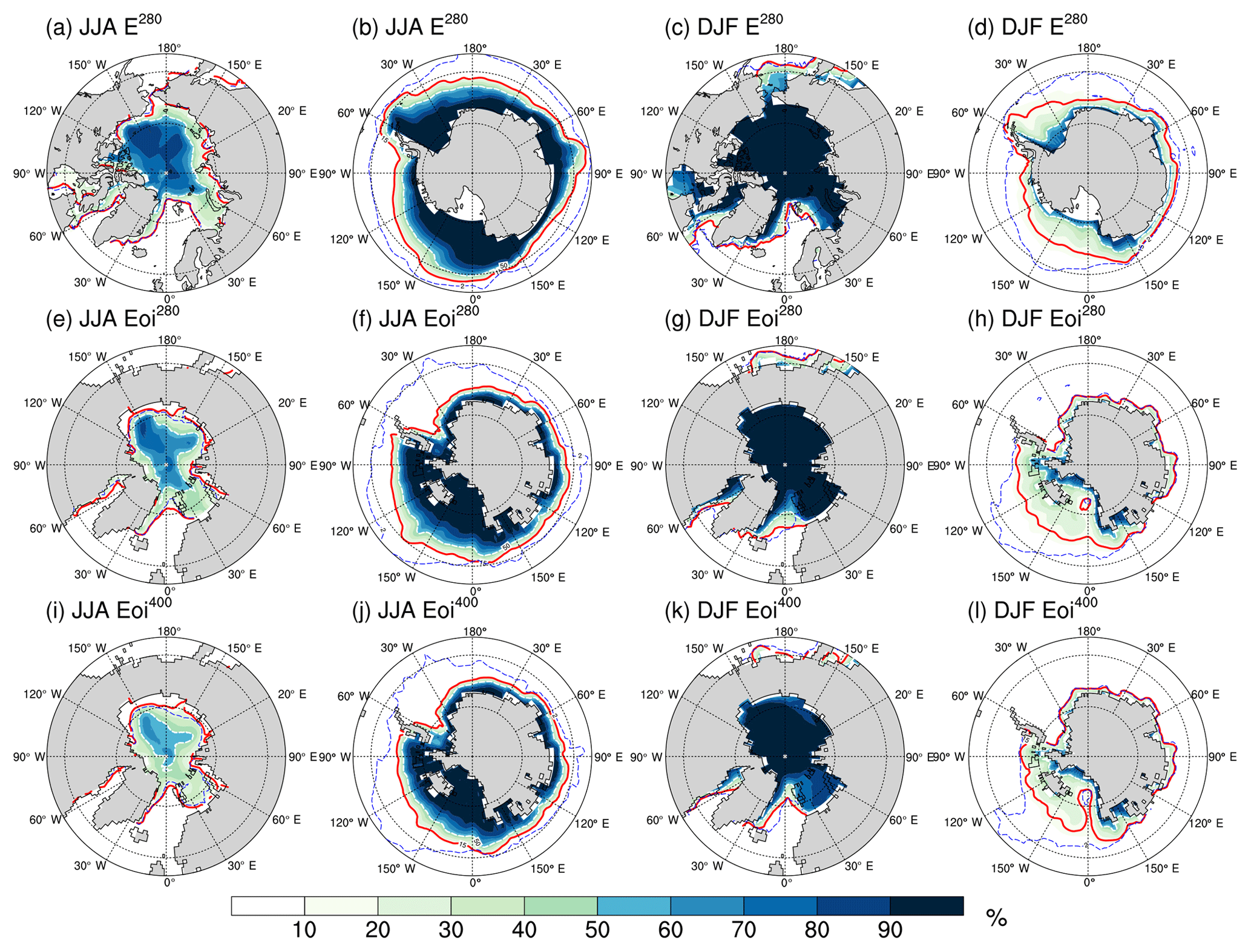
Figure 10 Sea ice concentrations (%) during JJA and DJF in the Northern and Southern Hemisphere for (a–d) E²⁸⁰, (e–h) Eoi²⁸⁰ and (i–l) Eoi⁴⁰⁰. The red line indicates the sea ice edge based on a threshold of 15 %, whilst the dotted white line indicates the 50 % threshold. The dotted blue line indicates the 2 ^∘C isotherm; in the Southern Ocean, this is indicative of the Antarctic convergence zone (polar front).

4.2.3 Mixed layer depth and deep-water formation

The mixed layer depth (MLD) for E²⁸⁰, Eoi²⁸⁰ and Eoi⁴⁰⁰ is shown within Fig. 11. We focus on deep convection, the principle mechanism of deep-water formation. Deep convection is highly localised, and therefore model representation is only suggestive. Nevertheless, E²⁸⁰ represents reasonably well the modern open-ocean deep convection that occurs within the Weddell and Ross seas (which form the main formation sites of AABW) and in the Labrador, Irminger and Greenland seas. All Pliocene experiments exhibit more widespread deep convection particularly within the Labrador and Norwegian seas, and near the Antarctic Peninsula island. In contrast to Burls et al. (2017), we do not model any significant increase in Pliocene North Pacific MLD and hence no subsequent intensification of North Pacific Deep Water (NPDW) formation (Table 7 and Fig. 11).

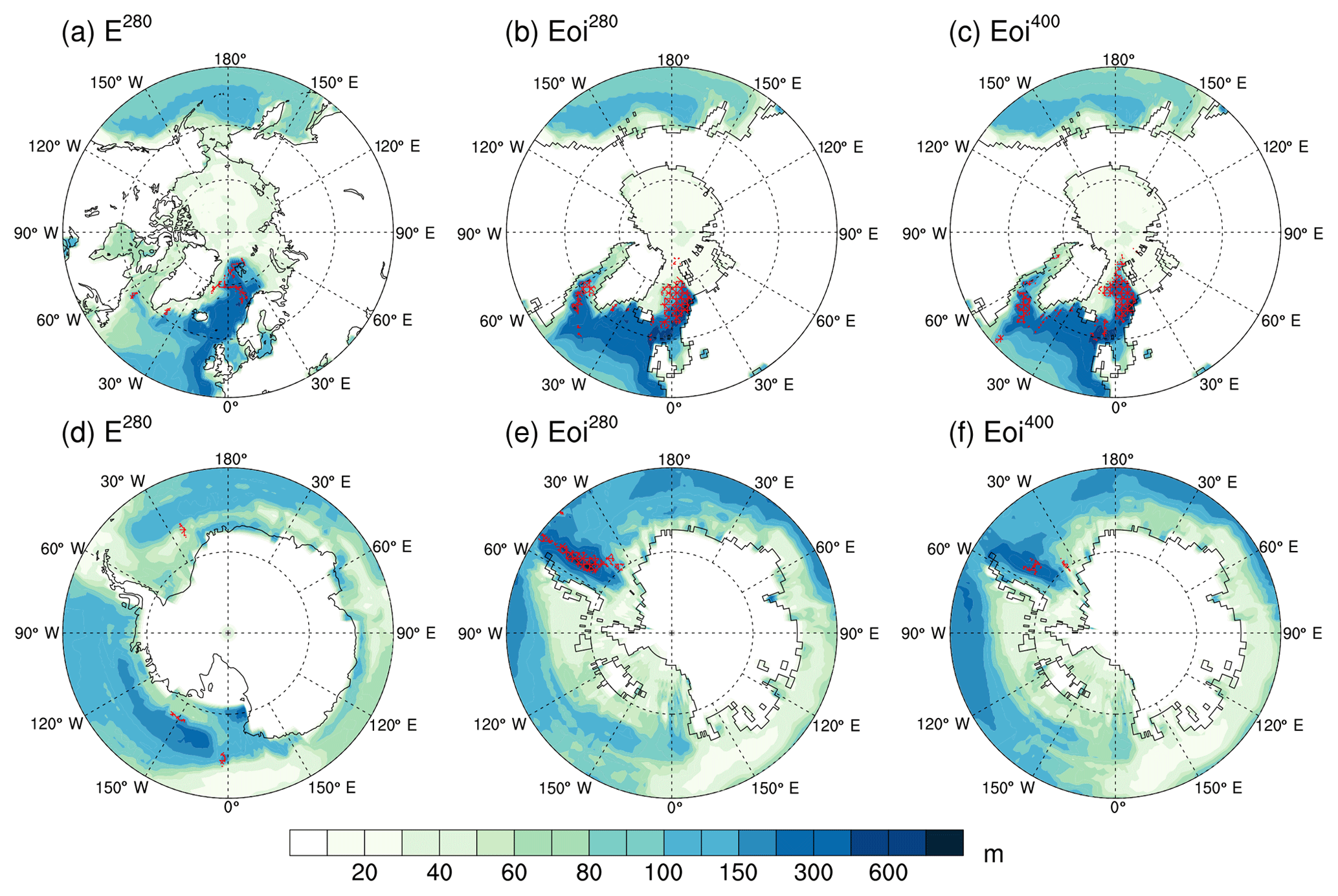
Figure 11 Mean March Northern Hemisphere and September Southern Hemisphere mixed layer depth for (a, d) E²⁸⁰, (b, e) Eoi²⁸⁰ and (c, f) Eoi⁴⁰⁰. Red hashes indicate regions that exhibit deep (>1000 m) convection at least 1 month during the climatological averaging period; single-cell ocean regions have been expanded slightly to improve visualisation.

4.2.4 Ocean heat and mass transport (Atlantic and Pacific MOCs)

The Atlantic meridional overturning circulation (AMOC) streamfunctions for E²⁸⁰, Eoi²⁸⁰ and Eoi⁴⁰⁰ are shown within Fig. 12 and detailed within Table 7. The pre-industrial experiment E²⁸⁰ has a maximum AMOC strength at 26.5^∘ N of 13.4±1.1 Sv. This compares reasonably well with the estimate of 17.2±4.6 Sv derived by McCarthy et al. (2015) using measurements from the RAPID array between April 2004 and October 2012. The all-latitude maximum in AMOC strength (AMOC_max) within E²⁸⁰ occurs at ∼650 m depth at 33.75^∘ N with a strength of15.7±1.2 Sv.

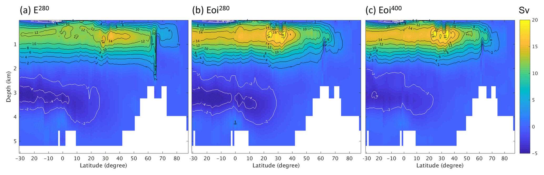
Figure 12 Time-averaged Atlantic overturning circulation for (a) E²⁸⁰, (b) Eoi²⁸⁰ and (c) Eoi⁴⁰⁰. Positive values indicate clockwise circulation.

We find an AMOC which is more intense in the Pliocene than in the pre-industrial, which is attributed to the Pliocene palaeogeography (Table 7). The AMOC_max of Eoi⁴⁰⁰ is 19.6 ± 1.0 Sv and occurs at ∼650 m depth at 33.75^∘ N. Multidecadal to centennial fluctuations within the spin-up phase are present within the Pliocene experiments but not within the pre-industrial experiment. In all Pliocene simulations, AMOC_max occurs within the 25–33.75^∘ N zonal envelope and at a depth of ∼650 m. The Eoi⁴⁰⁰ AMOC_max lies within the 10–24.6 Sv range of PlioMIP1 (Zhang et al., 2013), whilst the Eoi⁴⁰⁰–E²⁸⁰ AMOC_max anomaly of 3.9±1.6 Sv (Table 7) lies at the upper end of the PlioMIP1 ensemble range of −0.9–3.6 Sv. Despite an intensification of the AMOC within the Pliocene experiments, we find that the overturning strength reduces poleward of ∼40^∘ N driven by the changed land surface and bathymetry (Eoi²⁸⁰–E²⁸⁰). This is seen within cooling evident in Gulf Stream MASSTs of Fig. 9. Under increasing Pliocene CO₂, the midlatitude overturning intensifies with a corresponding decrease in the Gulf Stream MASST cold anomaly. The overturning within the polar region is evidence of bottom water formation within the Nordic Seas. In E²⁸⁰, overturning extends to ∼80^∘ N but is weaker than in the Pliocene experiments (which extends to ∼75^∘ N). This is reflected within the geographic extent and intensity of deep convection shown within Fig. 11.

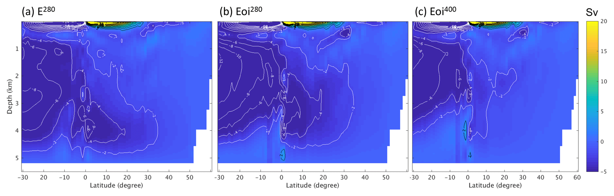
Figure 13 Time-averaged Pacific overturning circulation for (a) E²⁸⁰, (b) Eoi²⁸⁰ and (c) Eoi⁴⁰⁰. Positive values indicate clockwise circulation.

The Pacific meridional overturning circulation (PMOC) streamfunction is shown within Fig. 13 and detailed within Table 7, in which PMOC_+ve reflects the strength of the subtropical gyre circulation, whilst PMOC_−ve reflects the strength (and depth) of the Pacific Deep Water (PDW) and NPDW. Pliocene palaeogeography (Eoi²⁸⁰–E²⁸⁰) drives an intensification of both the subtropical gyre and PDW overturning, whilst increasing CO₂ acts to weaken them. The Pliocene subtropical gyre (PMOC_+ve) and PDW (PMOC_−ve) overturning are stronger regardless of CO₂ level (e.g. within Eoi⁴⁰⁰, PMOC_+ve and PMOC_−ve are 22 % and 6 % stronger than E²⁸⁰). With the change in palaeogeography (Eoi²⁸⁰–E²⁸⁰), the PDW shoals (from ∼4 to 3 km) and with increasing Pliocene CO₂ the NPDW overturning reduces in northward reach, associated with the warming of North Pacific MASST (Fig. 9).

4.2.5 Antarctic Circumpolar Current

The Antarctic Circumpolar Current (ACC) strength is detailed within Table 8 and shown within Fig. 14. We calculate the volumetric flow of the ACC at the Drake Passage across a 64.4–56.9^∘ S, 65^∘ W, transect using the positive aspect of the U component (zonal) of the total (barotropic and baroclinic) velocity. We find an overly intense ACC within E²⁸⁰ and E⁴⁰⁰ when compared against recent observations of 134–164 Sv (Cunningham et al., 2003; Griesel et al., 2012). The overly intense ACC within HadCM3 has been identified previously. Meijers et al. (2012) compared CMIP5 historical experiments to observations and found the model's ACC flow at the Drake Passage transect of 244.5±4.0 Sv compared unfavourably to observations and 155±51 Sv of the CMIP5 multi-model mean. This unrealistic intensity appeared to be driven, or at least connected to, an overly strong salinity gradient across the ACC, particularly towards low latitudes (Meijers et al., 2012). This could be a consequence of the artificial freshwater correction field used within the CMIP5 historical and piControl experiments and E²⁸⁰ here.

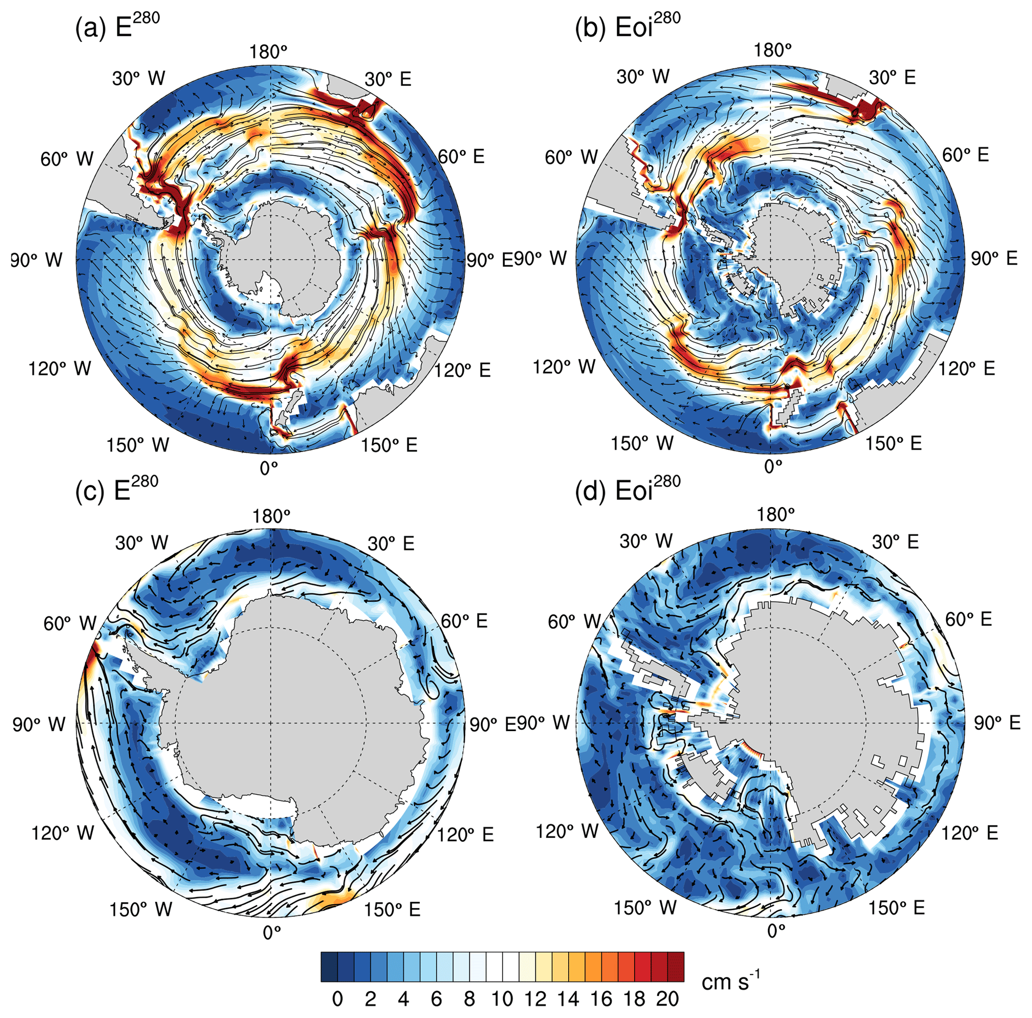
Figure 14 Surface ocean mean annual velocity (streamlines and vector magnitude) for E²⁸⁰ and Eoi²⁸⁰. The ACC is shown clearly within (a) E²⁸⁰ and (b) Eoi²⁸⁰, whilst the Antarctic Coastal Current is shown within the close-up plots of (c) E²⁸⁰ and (d) Eoi²⁸⁰.

Table 8 Characteristics of the Antarctic Circumpolar Current (ACC) within the Pliocene and pre-industrial experiments. From the barotropic streamfunction, we derive the mean ACC latitude (the polar front) from the centroid of the zonal transport and the core width from the ±50 % boundary.

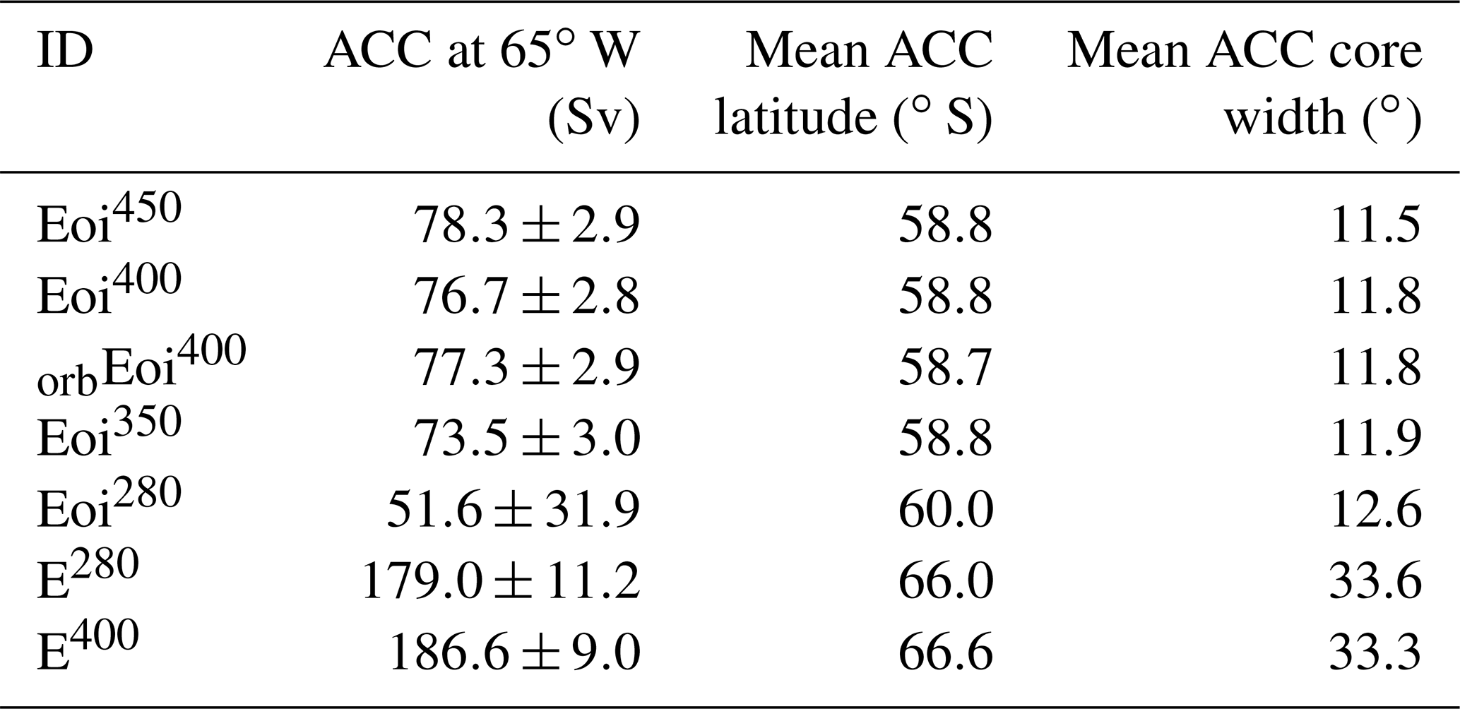
Modelled ACC strength appears significantly reduced within the Pliocene experiments. Westerlies intensify in the Southern Hemisphere within the Pliocene but mostly in regions poleward of the Sub-Antarctic front (poleward of the ACC). The weakened Drake Passage throughflow is mirrored within the vertically integrated barotropic streamfunction. Care must be taken when interpreting ACC strength in situations of changed palaeogeography and island specification. The ACC is weakly stratified and vertically coherent and so is dominantly barotropic in nature. Within the Pliocene boundary conditions (Sect. 3.2.2), the island peninsula is defined as a separate barotropic island (from the Antarctic continent), and this may be driving the Pliocene reduction in ACC strength. Also, given a more complex line-integral configuration, the model's barotropic solver may not be converging fully towards a solution. The change in island specification may also be responsible for the change in ACC geographical extent shown within Table 8. Defining the streamfunction cross section by the latitudes of the centroid and upper 50 % of zonal transport, we see that the change in geography (from E²⁸⁰ to Eoi²⁸⁰) drives a general latitudinal thinning of the ACC extent and an equatorward shift of its centroid.

Within the Pliocene experiments, the ACC runs mostly between the surface and sea floor between 60 and 57^∘ S, whilst a deeper countercurrent is present closer to the peninsula. In the Pacific, a pronounced thinning of the ACC latitude extent is observed whereby the Sub-Antarctic front moves equatorwards (the subtropical front is mostly unchanged). With the Pliocene geography, there are suggestions that the Antarctic Coastal Current (the countercurrent to the ACC) flows between the peninsula island and the Antarctic land mass. There is uncertainty as smaller islands in this region are unrepresented within the model. Figure 14 also suggests a more continuous coastal current with the Pliocene palaeogeography, particularly between 180 and 90^∘ E.

4.3 Sensitivity to external boundary conditions

4.3.1 Orbital configuration

Here, we examine the sensitivity of the Pliocene climate to a different choice of orbital configuration (e.g. modern (default) vs. KM5C at 3.205 Ma). For Eoi⁴⁰⁰, there is no meaningful difference in global means (Table 3 MASAT, Table 4 MAP, Table 6 MASST and warm pool areal extent).

There is a statistically significant difference between _orbEoi⁴⁰⁰ and Eoi⁴⁰⁰ AMOC_max (t(98)=7.20, p≪0.0001) and AMOC at 26.5^∘ N (t(98)=11.36, p≪0.0001) using a two-sample t test assuming unequal variance (null hypothesis being there is no difference in the two time series of annual means). With regards to PMOC_+ve, _orbEoi⁴⁰⁰ and Eoi⁴⁰⁰ are deemed equivalent (t(98)=0.62, p=0.54), whilst for PMOC_−ve, the two experiments are equivalent at the 95 % confidence level (t(98)=1.93, p=0.06). Centennial-scale fluctuations in Pliocene AMOC_max could potentially account for statistical differences between the climatological mean periods of _orbEoi⁴⁰⁰ and Eoi⁴⁰⁰, as AMOC_max differences could simply reflect a lack of coherence introduced since the year 2000 fork point.

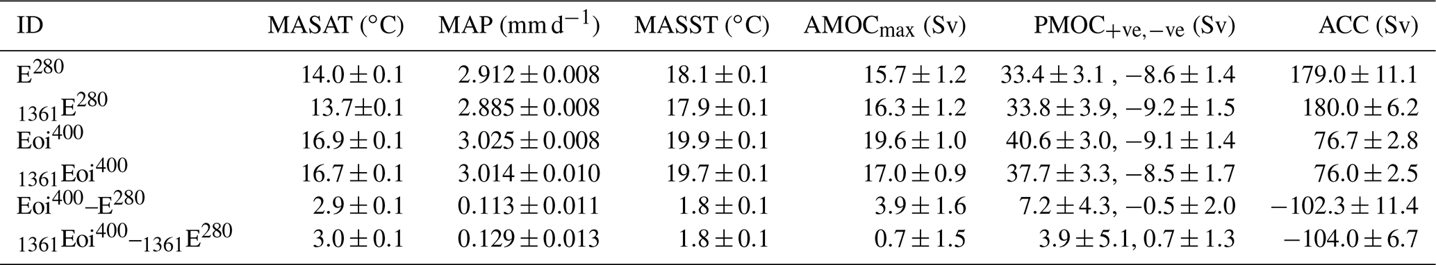
Table 9 Sensitivity of E²⁸⁰ and Eoi⁴⁰⁰ (and their corresponding anomalies) to TSI of 1361 and 1365 Wm⁻². Shown are the mean annual surface air temperature (MASAT), mean annual precipitation (MAP), mean annual sea surface temperature (MASST), Atlantic and Pacific meridional circulations (AMOC_max and PMOC${}_{+\mathrm{ve},-\mathrm{ve}}$; Sect. 4.2.4) and Antarctic Circumpolar Current (ACC; Sect. 4.2.5).

4.3.2 Total solar insolation

Section 2.1 identified the possibility of different TSI values being used within PlioMIP2 climate models. Here, we determine the sensitivity of HadCM3 within E²⁸⁰ and Eoi⁴⁰⁰ experiments to changing the TSI parameter. Reducing total solar insolation from 1365 to 1361 Wm⁻² (−0.3 %) reduces the mean incoming solar (SW) radiation averaged over the entire Earth's surface by 1 Wm⁻² (from 341.25 to 340.25 Wm⁻²). Table 9 accumulates climatological indices from E²⁸⁰ and Eoi⁴⁰⁰ under these two TSI values. Figure 15 shows the spatial pattern of climatological differences (Pliocene minus pre-industrial) for simulations based upon 1365 and 1361 Wm⁻² for MASAT, MAP and MASST. Overall the patterns of climatological anomalies for the experiments using TSI of either 1361 or 1365 Wm⁻² are very similar. In this sense, comparison of model temperature anomalies to proxy temperature anomalies should not generally be influenced by the choice of TSI.

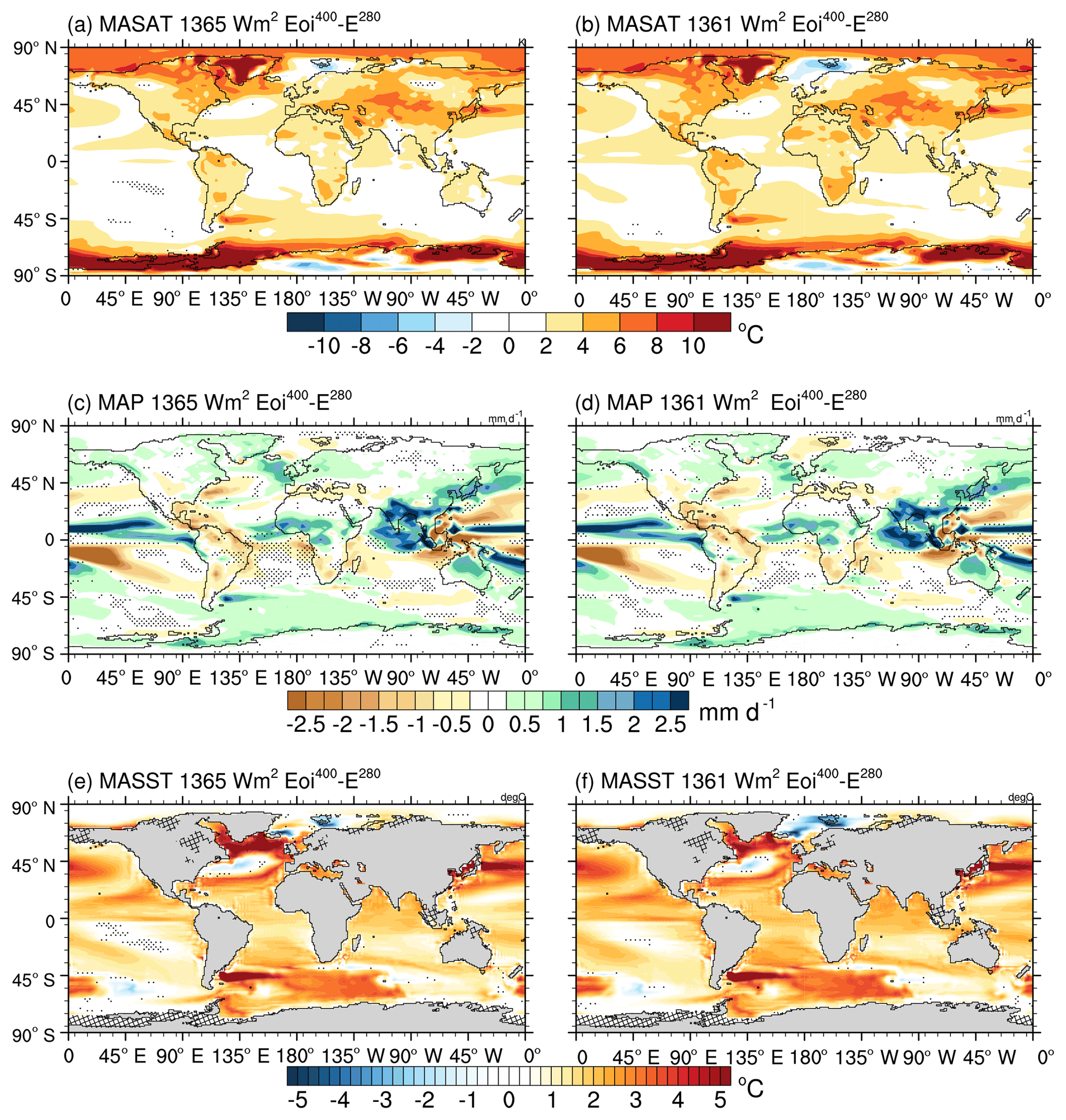
Figure 15 Sensitivity of Eoi⁴⁰⁰–E²⁸⁰ anomalies on TSI values for (a, b) MASAT, (c, d) MAP and (e, f) MASST. Stippling indicates regions in which results are not statistically significant at a 95 % confidence criterion.

However, in a similar way to the orbital configuration, AMOC_max does appear sensitive to TSI when we compare Eoi⁴⁰⁰ against ₁₃₆₁Eoi⁴⁰⁰ ($t\left(\mathrm{98}\right)=-\mathrm{13.3}$, p≪.0001) and E²⁸⁰ to ₁₃₆₁E²⁸⁰ (t(98)=2.47, p=0.015). It is possible that this sensitivity to TSI could be a consequence of the previously described AMOC cyclicity and lack of coherence between Eoi⁴⁰⁰ and ₁₃₆₁Eoi⁴⁰⁰.

5 Discussion

In this study, we have described the incorporation of PlioMIP2 (PRISM4) mid-Piacenzian (Pliocene) enhanced boundary conditions into the HadCM3 global climate model. We conducted PlioMIP2 CORE and tier 1 pre-industrial and Pliocene-based experiments as well as sensitivity experiments exploring solar insolation and orbit choice. We then examined the large-scale features of the atmosphere and ocean state of these experiments.

Compared to the pre-industrial control (E²⁸⁰), we find Pliocene surface warming focussed within the high latitudes and whose spatial distribution is similar to that obtained with HadCM3 for PlioMIP1 under PRISM3 boundary conditions (Bragg et al., 2012). We find that the Pliocene palaeogeography and 400 ppm CO₂ account for a warming (relative to the pre-industrial) in globally integrated MASAT (and MASST) of 1.4 (0.8 ^∘C) and 1.5 ^∘C (1.0 ^∘C), respectively. We derive climate sensitivities of 3.5 and 2.9 ^∘C per doubling of CO₂ for the pre-industrial and Pliocene, which are also similar to results from PlioMIP1 wherein they were estimated to be 3.3 and 3.1 ^∘C, respectively (Haywood et al., 2013b). We estimate the Earth system sensitivity at ∼5.6 ^∘C, implying an ESS ∕ CS ratio of ∼1.9, which is similar to the ESS ∕ CS ratio of 2.0 derived within PlioMIP1 (Haywood et al., 2013b). This similarity between PlioMIP1 and PlioMIP2 CS and the ESS ∕ CS ratio demonstrates an insensitivity of these quantities to the degree of palaeogeographic variation between PlioMIP1 and PlioMIP2. This strongly indicates that the primary control on the ESS ∕ CS ratio is the reconstructed ice distribution and global vegetation coverage which, with the exception to the Greenland Ice Sheet, is consistent between PlioMIP1 and PlioMIP2. The implementation of dynamic global vegetation models by PlioMIP2 participant groups will allow investigation of the sensitivity of ESS ∕ CS to vegetation–climate feedbacks. We also recognise that CS and ESS calculations are model dependent and this will be looked at in detail in the multi-model comparison of PlioMIP2 results. Precipitation change is more complex. Pliocene geography is the primary driver of geographical distribution changes in precipitation, whilst both Pliocene geography and CO₂ increase the globally integrated MAP.

We find an AMOC which is more intense in the Pliocene than in the pre-industrial, with the variation driven principally by the change in geography (Table 7). We determine this by comparing AMOC strength of E²⁸⁰ against Eoi⁴⁰⁰ and Eoi²⁸⁰. In addition, we have explored the sensitivity of AMOC strength to methodology applied for freshwater correction. The Eoi²⁸⁰ experiment uses a fixed freshwater correction field corresponding to pre-industrial iceberg trajectories, whilst the Pliocene experiment uses an annually derived correction (Sect. 2.2). In theory, this could impact on simulated AMOC intensity in Eoi⁴⁰⁰ vs. E²⁸⁰. To test this, we have conducted an additional E²⁸⁰ experiment using the annually derived freshwater correction methodology of Eoi⁴⁰⁰ (results not shown). This has demonstrated for the pre-industrial that the freshwater correction method does not lead to a statistically different AMOC strength. This indicates that our intensified AMOC within Eoi⁴⁰⁰ is indeed a consequence of palaeogeographic changes, rather than our approach to freshwater correction.

Both the choice of TSI (1361 vs. 1365 Wm⁻²) and PRISM4 orbital configuration (modern vs. 3.205 Ma) have been shown not to significantly influence the anomaly-type analysis in use by the Pliocene community. For example, we show that the representation of the KM5c (3.205 Ma) time slice with a modern orbit is an acceptable choice – leading to no statistically significant differences within MASAT (Table 3) or MAP (Table 4), which is in accordance with previous work (Haywood et al., 2013a). When considering absolute values or climatic indices, the influence of TSI or orbit is minimal but should nevertheless be considered. Models with greater climate sensitivity will present more sensitivity to TSI and potential for non-linearities in climate response (e.g. relating to feedbacks at or near the sea ice edge or climate–vegetation interactions).

Whilst the Pliocene represents an incredibly useful contemporary-climate analogue, the use of a non-modern palaeogeography (enhanced PRISM4 boundary condition dataset) does present limitations when using low to intermediate spatial resolution climate models. Regridding of the LSM to the $\mathrm{3.75}{}^{\circ }\times \mathrm{2.5}{}^{\circ }$ model is imperfect due to the binary nature of the data and therefore requires manual corrections driven by an understanding of model architecture and physics (i.e. imposed by rigid-lid streamfunction, horizontal grid type, etc.). As a precursor, some a priori knowledge of important aspects of Pliocene ocean circulation is required to guide a series of expert-informed decisions on model configuration. Similarly, when model development teams (e.g. MOHC) create present-day boundary conditions, knowledge of circulation patterns and throughflow strength is often used to inform manual corrections (e.g artificial deepening of narrow channels) or the inclusion of parameterisations (e.g. diffusive pipes to represent, otherwise unrepresented, narrow straits). This a priori knowledge is not necessarily available for the Pliocene, and it is therefore difficult to assess. An example of this is in the subaerial extension of Ireland and Scotland within PRISM4, posing the question of how this region should be represented within the model and how the model representation may influence the simulation of the Norwegian Current. Additionally, the use of different model architectures and models with higher spatial resolution within the PlioMIP2 framework may allow these aspects to be considered. For example, free-surface ocean models with higher horizontal spatial resolution may help in the interpretation of the Pliocene ACC strength and the Pliocene Arctic Ocean cold anomaly identified within this study.

Palaeogeography-induced changes in mean state, for example, the path of the Antarctic Coastal Current around the peninsula island (Sect. 4.2.5), represent potentially non-analogous characteristics imposed by the PRISM4 Pliocene reconstruction. Other non-analogous changes are associated with palaeogeographical changes to the maritime continent and subsequent changes in Indonesian throughflow configuration, the closure of the Bering Strait and Canadian Archipelago, and the withdrawal of the Baltic Sea and Hudson Bay. These palaeogeographical changes should be considered alongside those described within Hill (2015), such as the suggestion of extensive uplift in the Barents Sea (e.g. Knies et al., 2014) and the rerouting of major rivers (e.g. within North America), which may be currently unrepresented within the model. These important regional changes must be appreciated when considering the KM5c time slice as an equilibrium state analogue to contemporary-climate change (i.e. a 400 ppm world).