Coupled climate–carbon cycle simulation of the Last Glacial Maximum atmospheric CO₂ decrease using a large ensemble of modern plausible parameter sets

During the Last Glacial Maximum (LGM), atmospheric CO₂ was around 90 ppmv lower than during the pre-industrial period. The reasons for this decrease are most often elucidated through factorial experiments testing the impact of individual mechanisms. Due to uncertainty in our understanding of the real system, however, the different models used to conduct the experiments inevitably take on different parameter values and different structures. In this paper, the objective is therefore to take an uncertainty-based approach to investigating the LGM CO₂ drop by simulating it with a large ensemble of parameter sets, designed to allow for a wide range of large-scale feedback response strengths. Our aim is not to definitely explain the causes of the CO₂ drop but rather explore the range of possible responses. We find that the LGM CO₂ decrease tends to predominantly be associated with decreasing sea surface temperatures (SSTs), increasing sea ice area, a weakening of the Atlantic Meridional Overturning Circulation (AMOC), a strengthening of the Antarctic Bottom Water (AABW) cell in the Atlantic Ocean, a decreasing ocean biological productivity, an increasing CaCO₃ weathering flux and an increasing deep-sea CaCO₃ burial flux. The majority of our simulations also predict an increase in terrestrial carbon, coupled with a decrease in ocean and increase in lithospheric carbon. We attribute the increase in terrestrial carbon to a slower soil respiration rate, as well as the preservation rather than destruction of carbon by the LGM ice sheets. An initial comparison of these dominant changes with observations and paleoproxies other than carbon isotope and oxygen data (not evaluated directly in this study) suggests broad agreement. However, we advise more detailed comparisons in the future, and also note that, conceptually at least, our results can only be reconciled with carbon isotope and oxygen data if additional processes not included in our model are brought into play.

1 Introduction

Analyses of Antarctic ice core records suggest that the atmospheric CO₂ concentration at the Last Glacial Maximum (LGM), about 21 kyr ago, was around 190 ppmv, well below the pre-industrial atmospheric concentration of around 280 ppmv. The most commonly accepted mechanisms to explain the atmospheric CO₂ decrease include lower sea surface temperatures, which increase the ocean CO₂ solubility (Martin et al., 2005; Menviel et al., 2012), enhanced ocean biological pump due to increased input of aeolian iron to the ocean (Bopp et al., 2003; Oka et al., 2011; Jaccard et al., 2013; Ziegler et al., 2013; Martínez-García et al., 2014; Lambert et al., 2015), capping of air–sea gas exchange by expanding sea ice (Stephens and Keeling, 2000; Sun and Matsumoto, 2010; Chikamoto et al., 2012) and ocean circulation/stratification changes increasing the net CO₂ flux into the ocean (Adkins et al., 2002; Lynch-Stieglitz et al., 2007; Skinner et al., 2010, 2014; Lippold et al., 2012; Gebbie, 2014; Tiedemann et al., 2015; de la Fuente et al., 2015; Freeman et al., 2015). These changes may in turn be due to a range of possible mechanisms such as increased brine rejection (Shin et al., 2003; Bouttes et al., 2010, 2011; Zhang et al., 2013; Ballarotta et al., 2014), a shift in/weakening of the westerly wind belt over the Southern Ocean (Toggweiler et al., 2006; Anderson et al., 2009; Völker and Köhler, 2013) and a reduced or reversed buoyancy flux from the atmosphere to the ocean surface in the Southern Ocean (Watson and Naveira Garabato, 2006; Ferrari et al., 2014). A process that is conversely assumed to have contributed to increasing atmospheric CO₂ is increasing salinity and ocean total dissolved inorganic carbon (DIC) concentration in response to decreasing sea level (Ciais et al., 2013).

A dominant assumption is also that the terrestrial biosphere carbon inventory was reduced (Crowley, 1995; Adams and Faure, 1998; Ciais et al., 2012; Peterson et al., 2014), in line with independent estimates of an ocean carbon inventory that was enhanced by several hundred petagrams (Goodwin and Lauderdale, 2013; Sarnthein et al., 2013; Allen et al., 2015; Skinner et al., 2015; Schmittner and Somes, 2016). The decrease in terrestrial carbon is generally attributed to unfavourable climatic conditions for photosynthesis and the destruction of organic material by moving ice sheets (e.g. Otto et al., 2002; Prentice et al., 2011; Brovkin et al., 2012; O'ishi and Abe-Ouchi, 2013). The hypothesis that there was an increase in terrestrial carbon has, however, also been put forward (e.g. Zeng, 2003; Zimov et al., 2006), with some studies additionally suggesting little net change (e.g. Brovkin and Ganopolski, 2015). Processes proposed to be responsible for the terrestrial carbon increase include growth in “inert” or permafrost carbon, slower “active” soil respiration rates, continental shelf regrowth and the preservation rather than destruction of terrestrial biosphere carbon in areas to be covered by the expanding Laurentide and Eurasian ice sheets (Weitemeyer and Buffett, 2006; Franzén and Cropp, 2007; Zeng, 2007; Zimov et al., 2009; Zech et al., 2011).

Other mechanisms which may have affected the LGM atmospheric CO₂ change include changes in carbonate weathering rate, through its control on the ocean ALK:DIC ratio and consequently the solubility of CO₂ (Munhoven, 2002; Jones et al., 2002; Foster and Vance, 2006; Vance et al., 2009; Brovkin et al., 2012; Crocket et al., 2012; Lupker et al., 2013; Simmons et al., 2016). The change in carbonate weathering rate would in turn have been caused by lower sea level, exposing previously submerged rock, the presence of a greater amount of glacial flour, which is more susceptible to weathering (Kohfeld and Ridgwell, 2009), or potentially higher soil carbon content. The lower sea level may also have reduced shallow water carbonate deposition by decreasing the area of shallow ocean (Opdyke and Walker, 1992; Kleypas, 1997; Brovkin et al., 2007), and increased oceanic PO₄ inventory, alleviating the PO₄ limitation on marine production (Tamburini and Föllmi, 2009; Wallmann, 2014, 2015). Other potential CO₂ mechanisms include decreasing dissolved organic carbon inventory due to a more stratified deep ocean (Ma and Tian, 2014) and reduced marine bacterial metabolic rate in response to lower ocean temperatures. The lower metabolic rate acts to decrease the return rate of DIC from the remineralisation of organic material and hence the concentration of CO₂ at the ocean surface (Matsumoto et al., 2007; Roth et al., 2014). The net flux of CO₂ into the ocean may also have increased due to enhanced diatom production caused by the leakage of silicic acid trapped in the Southern Ocean (Matsumoto et al., 2002, 2014) or increased Si inventory, caused by increased input of Si from wind-born dust or enhanced weathering (Harrison, 2000; Tréguer and Pondaven, 2000).

Mechanisms put forward to explain the LGM atmospheric CO₂ decrease arise from paleodata and model studies. The latter most often involve factorial experiments, introducing mechanisms one at a time. There is rarely any investigation of the impact of alternative assumptions regarding parameter values or model structure. An example of a relevant study is Bouttes et al. (2011), which varied model parameters controlling the importance of iron fertilisation, brine rejection and stratification-dependent diffusion in an ensemble setting, assessing the agreement of the model output with data. Here, our aim is conversely to take an uncertainty-based approach to investigating the LGM CO₂ drop by simulating it with a large ensemble of parameter sets designed to allow for a wide range of large-scale feedback response strengths (Holden et al., 2013a). The objective is not to definitely explain the causes of the CO₂ drop but rather explore the range of possible responses. By “responses” we mean physical and biogeochemical changes in the Earth system (e.g. change in global particulate organic carbon export flux) and how these might be linked to ΔCO₂ and to each other, rather than specific mechanisms (e.g. iron fertilisation). Knowledge of these relationships can in turn inform analysis, in the future, of the relationship between the ensemble parameters and model outputs, in order to isolate individual LGM CO₂ mechanisms. In this study, we furthermore seek to simulate the LGM atmospheric CO₂ drop with the simulated CO₂ feeding back to the simulated climate, which is still infrequently done in LGM CO₂ experiments, and the first time it is done with GENIE-1. Moreover, rather than assuming that terrestrial carbon is destroyed by the LGM ice sheets, we assume that it is gradually buried. This assumption has not yet been implemented, in GENIE-1 or other models, in an equilibrium set-up.

Despite our ensemble varying many of the parameters thought to contribute to variability in glacial–interglacial atmospheric CO₂, not all sources of uncertainty can be captured, and this is reflected in our simulated ΔCO₂ distribution. We estimate that up to ∼60 ppmv of ΔCO₂ could be due to processes not included in our model and error in our process representations (see Sect. 2.4 for details). We thus treat ΔCO₂ between $\sim -\mathrm{90}$ and −30 ppmv as “equally plausible” and focus on describing the physical and biogeochemical changes seen in the subset of simulations with this ΔCO₂. We also conduct an initial assessment of how the subset mean and/or dominant (in terms of sign) responses compare against observations and paleoproxies, including temperature, sea ice, precipitation, AMOC and AABW cell strengths, terrestrial carbon, ocean carbon, particulate organic matter export and deep-sea CaCO₃ burial.

Finally, to test the robustness of relationships derived from the analysis of the ensemble subset with ΔCO₂ between $\sim -\mathrm{90}$ and −30 ppmv, we briefly compare the physical and biogeochemical changes seen therein with the changes seen in the ensemble with no ΔCO₂ filter and the ensemble with a more negative ΔCO₂ filter ($\sim -\mathrm{90}$ to −60 ppmv) (Sect. 2.4). In general, the same dominant relationships between ΔCO₂ and the physical and biogeochemical changes are observed as in the subset with ΔCO₂ between $\sim -\mathrm{90}$ and −30 ppmv. In the case of the ensemble subset with ΔCO₂ between $\sim -\mathrm{90}$ and −60 ppmv, we additionally look at what proportion of the total terrestrial carbon change comes from within the ice sheet areas and from there draw conclusions for the rest of the ensemble.

The paper is organised as follows. Section 2 describes the model, the ensemble, the simulation set-up and the ensemble subsets to be analysed. Section 3 is the results and discussion section, which includes a brief evaluation of the pre-industrial (control) spin-up simulation to verify reproducibility of Holden et al. (2013a). The majority of the section is devoted to the LGM simulation: namely, diagnosis of the physical and biogeochemical changes (including potential causal relationships) seen in the subset with ΔCO₂ between $\sim -\mathrm{30}$ and −90 ppmv, and to a lesser extent, the ensemble with both more and less constrained ΔCO₂. Comparison of the first subset against observations and paleoproxies is also included. Section 4 provides the key conclusions.

2 Methods

2.1 The model

The GENIE-1 configuration is as described in Holden et al. (2013a). The physical model consists of a three-dimensional frictional geostrophic ocean model (GOLDSTEIN) coupled to a thermodynamic/dynamic sea ice model (Edwards and Marsh, 2005; Marsh et al., 2011) and a two-dimensional Energy–Moisture Balance Model (EMBM). Atmospheric tracers are a subcomponent of the EMBM, with a simple module (ATCHEM) used to store the concentration of atmospheric gases and their relevant isotopic properties (Lenton et al., 2007). The model land surface physics and terrestrial carbon cycle are represented by an efficient numerical terrestrial scheme (ENTS) (Williamson et al., 2006). The ocean biogeochemistry model (BIOGEM) is as described in Ridgwell et al. (2007) but includes a representation of iron cycling (Annan and Hargreaves, 2010) and the biological uptake scheme of Doney et al. (2006). The model sediments are represented by SEDGEM (Ridgwell and Hargreaves, 2007). GENIE-1 also includes a land surface weathering model, ROKGEM (Colbourn, 2011), which redistributes prescribed weathering fluxes according to a fixed river-routing scheme. The model is on a 36×36 equal-area horizontal grid, with 16 vertical levels in the ocean.

2.2 The simulation ensemble

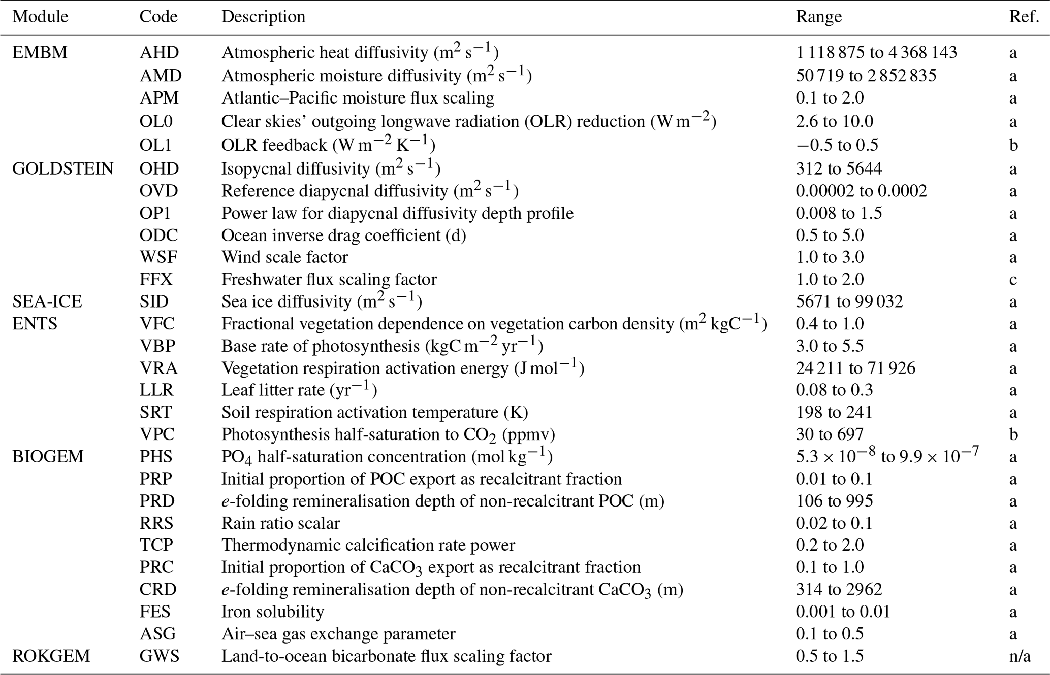
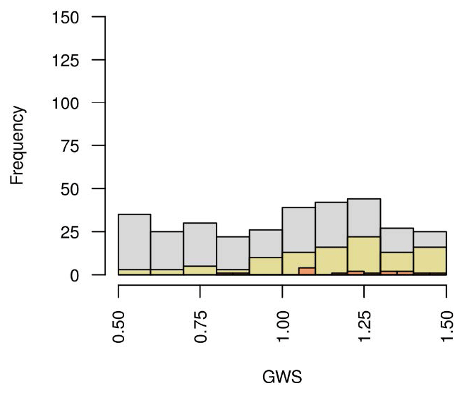
The GENIE-1 ensemble consists of 471 parameter sets, varying 29 key model parameters over the ranges in Table 1. It derives from the 471-member emulator-filtered plausibility constrained ensemble of Holden et al. (2013a), which varies 24 active parameters and 1 dummy parameter (as a check against overfitting). The parameter values in Holden et al. (2013a) were derived by building emulators of eight pre-industrial climate metrics and applying a rejection sampling method known as approximate Bayesian computation (ABC) to find parameter sets that the emulators predicted were modern plausible. Two parameters were later added to the ensemble, in Holden et al. (2013b), to describe the unmodelled response of clouds to global average temperature change (OL1) (see Appendix A for further information) and the uncertain response of photosynthesis to changing atmospheric CO₂ concentration (VPC). The parameters are as described in Holden et al. (2013b). We add two further parameters here that represent uncertain processes specific to the LGM. The first (FFX) scales ice sheet meltwater fluxes to account for uncertainty in unmodelled isostatic depression at the ice–bedrock interface due to ice sheet growth and for assuming a fixed land–sea mask (Holden et al., 2010b). We vary the parameter in the ensemble to capture the uncertainty in the magnitude of the glacial sea level drop and its effects on the carbon cycle. The second (GWS) scales the global average pre-industrial carbonate weathering rates for the LGM, to account for uncertainty in carbonate weathering and unmodelled shallow water carbonate deposition rate changes. For both FFX and GWS, uniform random values were derived using the generation function “runif” in R.

Table 1 Ensemble parameters. Ranges are from (a) Holden et al. (2013a), (b) Holden et al. (2013b) and (c) Holden et al. (2010b), with the exception of GWS (see main text). The table also precludes the dummy parameter.

n/a – not applicable

2.3 Experimental set-up of the model

The pre-industrial ensemble simulation results were repeated to verify reproducibility of Holden et al. (2013a). The simulations were performed in two stages, each lasting 10 kyr, on the Cambridge high-performance computing (HPC) cluster Darwin. The first stage involved spinning up the model with atmospheric CO₂ concentration relaxed to 278 ppmv and a closed biogeochemistry system. This means that there are no sediment–ocean interactions and the model forces the CaCO₃ weathering and deep-sea sediment burial rates into balance. An initial CaCO₃ weathering flux is prescribed, but this is subsequently rescaled internally to balance the modelled CaCO₃ burial rate and conserve alkalinity. In the second stage, atmospheric CO₂ was allowed to evolve freely, with interacting oceans and sediments, and the CaCO₃ weathering rate is set equal to the CaCO₃ burial rate diagnosed from the end of stage 1. To allow the sediments to reach equilibrium as fast as possible, no bioturbation was modelled in either stage 1 or stage 2.

Each parameter set was then applied to LGM simulations. The modelled pre-industrial equilibrium states were used as initial conditions and the ensemble members were integrated for 10 kyr, with freely evolving CO₂. These 10 kyr simulations are variously referred to here as the “LGM equilibrium simulation” or “stage 3”, and the LGM equilibrium state refers to the end of stage 3 (see Sect. S1 in the Supplement for more details). After application to stages 2 and 3, the original 471 ensemble members were filtered to 315 ensemble members to exclude those simulations with a stage 2 atmospheric CO₂ concentration outside of the range 268 to 288 ppmv (see Prentice et al., 2001), those that entered a snowball Earth state in stage 3 (global annual SAT between $\sim -\mathrm{68}$ and −57 ^∘C) or those that showed evidence of numerical instability (see Holden et al., 2013b).

Boundary conditions applied in the LGM simulations included orbital parameters (Berger, 1978) and aeolian dust deposition fields (Mahowald et al., 2006). The atmospheric CO₂ used in the radiative code is internally generated, rather than prescribed, but the radiative forcing from dust and gases other than CO₂ was neglected. The model also requires a detrital flux field to the sediments, containing contributions from opal and material from non-aeolian sources (Ridgwell and Hargreaves, 2007). Weathering fluxes from the pre-industrial simulation were applied, scaled by GWS (the land-to-ocean bicarbonate flux scaling factor).

The representation of the ice sheets is as described in Holden et al. (2010b), using the terrestrial ice sheet fraction and orography from the ICE-4G reconstruction of Peltier (1994). Rather than initialising the ensemble with the ice sheet extent and orography at 21 kyr BP, the ice sheets are configured to grow from their pre-industrial to LGM extent in 1 kyr, at the beginning of the LGM simulation (i.e. 0–1 kyr) in order to account for the impact of sea level change on ocean tracers. Following Holden et al. (2010b), only the Laurentide and Eurasian ice sheets are allowed to change from their pre-industrial form (accounting for ∼80 % of global ice sheet change), and we also route the freshwater to build the ice sheets from the Atlantic, Pacific and Arctic, assuming modern topography, rather than extracting it uniformly. As the ice sheets grow, grid cells on land are gradually covered by ice, and any carbon that remains, or has accumulated, is preserved underneath (“buried”). Once the ice covers a grid cell, there is no more exchange between the land carbon in that grid cell and the atmosphere. Prior to being buried, however, it is subject to the same forcings as carbon in any other grid cell. To determine how sensitive the burial carbon amount (i.e. the amount of carbon that is available for preservation underneath the ice) is to the duration of ice sheet build-up, we test the impact of varying the latter from 1 to 10 kyr for one ensemble member (extending the total simulation length to 11 kyr). Our assumption is that if the difference is negligible, applying the same ensemble member to a transient simulation of the full glacial cycle (and therefore a more realistic ice sheet build-up history) would not have yielded a dramatically different burial carbon inventory. We find that increasing the ice sheet build-up duration indeed changes the burial carbon amount only marginally: an increase of ∼34 PgC. A limitation, however, is that we do not have a way of testing if the response of other ensemble members would be equally subdued.

2.4 Ensemble subsets

Although our ensemble varies many of the parameters thought to contribute to variability in glacial–interglacial atmospheric CO₂, not all sources of uncertainty can be captured. We estimate, based on our expert opinion, that up to ∼60 ppmv of ΔCO₂ could be due to error in our process representations and processes not included in our model, such as changing marine bacterial metabolic rate, wind speed (via its effect on gas transfer) and Si fertilisation. This is not a comprehensive assessment, however, as our model also does not include processes such as the effect of changing winds on ocean circulation (Toggweiler et al., 2006), Si leakage (Matsumoto et al., 2002, 2013, 2014), the effect of decreasing sea surface temperatures (SSTs) on CaCO₃ production (Iglesias-Rodriguez et al., 2002) or changing oceanic PO₄ inventory (Menviel et al., 2012). We focus our analyses on the subset of the ensemble with ΔCO₂ between $\sim -\mathrm{90}$ and −30 ppmv (Table 2), treating each value in this range as equally plausible. To test the robustness of diagnosed relationships, we also briefly compare the response of this subset (ENS₁₀₄) with the response of the ensemble with no ΔCO₂ filter (ENS₃₁₅) and the response of the ensemble with a more negative ΔCO₂ filter (ENS₁₆). In ENS₁₆, the upper ΔCO₂ limit is set to $\sim -\mathrm{60}$ ppmv, roughly equivalent to allowing for an extra atmospheric CO₂ decrease due to changing marine bacterial metabolic rate, wind speed (via its effect on gas transfer) and Si fertilisation, between the best and upper estimate of Kohfeld and Ridgwell (2009). The ΔCO₂ distribution in each subset or ensemble is shown in Fig. 1.

Table 2 Ensemble subsets, including ΔCO₂ and number of members in each.

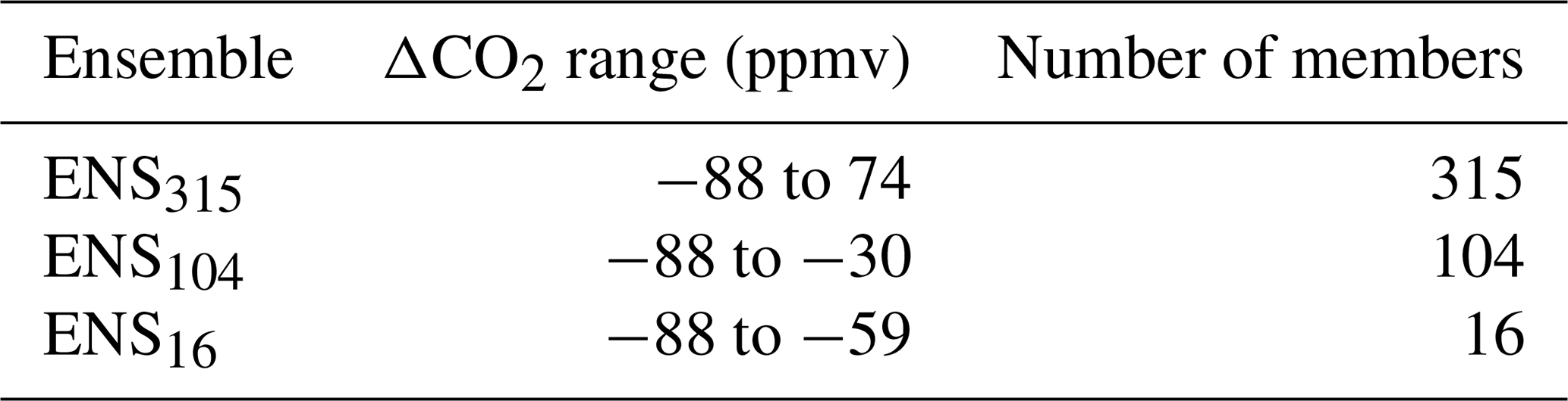
Figure 1 LGM change in atmospheric CO₂ distribution. The ENS₃₁₅ response is shown in grey, the ENS₁₀₄ ensemble response in yellow and the ENS₁₆ ensemble response in orange. The same colour legend applies to all figures in the paper.

3 Results and discussion

3.1 Pre-industrial simulations

Comparison of the pre-industrial response of ENS₃₁₅ (i.e. the original, non-ΔCO₂ filtered ensemble) against the pre-industrial ensemble response of Holden et al. (2013a) confirms that the two are very similar. We additionally evaluate ENS₃₁₅ against a few additional pre-industrial metrics (see Sect. S2) and find responses that can be deemed plausible, following the design principles for the ensemble, outlined in Holden et al. (2013a).

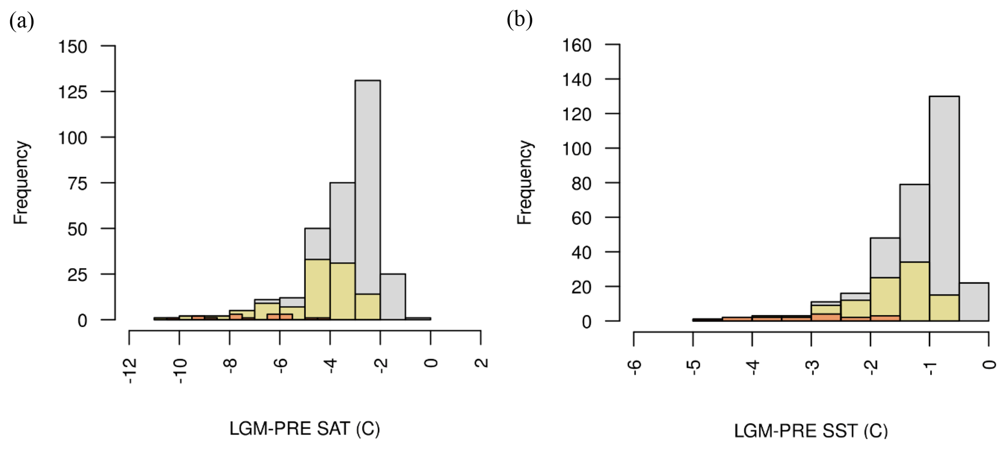
Figure 2 LGM change in surface air temperature and sea surface temperature (a–b) distributions.

3.2 LGM simulations

3.2.1 Climate, sea level and ocean circulation

Temperature

The ENS₁₀₄ mean LGM surface air temperature (SAT) anomaly (ΔSAT) is $-\mathrm{4.6}\pm \mathrm{1.7}$, and the range is −2.5 to −10.4 ^∘C. The mean is close to the observed ΔSAT of $-\mathrm{4}\pm \mathrm{1}$ ^∘C (Annan and Hargreaves, 2013) and the range roughly equivalent to the range of previous model-based estimates (Kim et al., 2003; Masson-Delmotte et al., 2006; Schneider von Deimling et al., 2006; Braconnot et al., 2007; Holden et al., 2010a; Brady et al., 2013). The ENS₁₀₄ mean LGM SST anomaly (ΔSST) is $-\mathrm{1.8}\pm \mathrm{0.8}$ ^∘C, and the range is −4.5 and −0.7 ^∘C. The mean is again close to an observational data-constrained model estimate (Schmittner et al., 2011) and within the range of estimates inferred from proxy data (MARGO Project Members 2009 in Masson-Delmotte et al., 2013). There is a positive correlation between ΔSAT and ΔCO₂ (r=0.75, 0.05 significance level henceforth), most likely reflecting the radiative impact of atmospheric CO₂ on SAT, as well as the effect of changing SAT on ΔCO₂. As suggested above, decreasing SST may contribute to decreasing CO₂ via the CO₂ solubility temperature dependence. Changing SAT may also affect ΔCO₂ via its effects on sea ice, ocean circulation, terrestrial and marine productivity (see below). The positive correlation is reproduced in ENS₃₁₅ (r=0.74), and as shown in Fig. 2, ΔSAT and ΔSST tend to be less negative in ENS₃₁₅ than in ENS₁₀₄. In ENS₁₆, ΔSAT and ΔSST are from the extreme or at least lower end of the ENS₁₀₄ range.

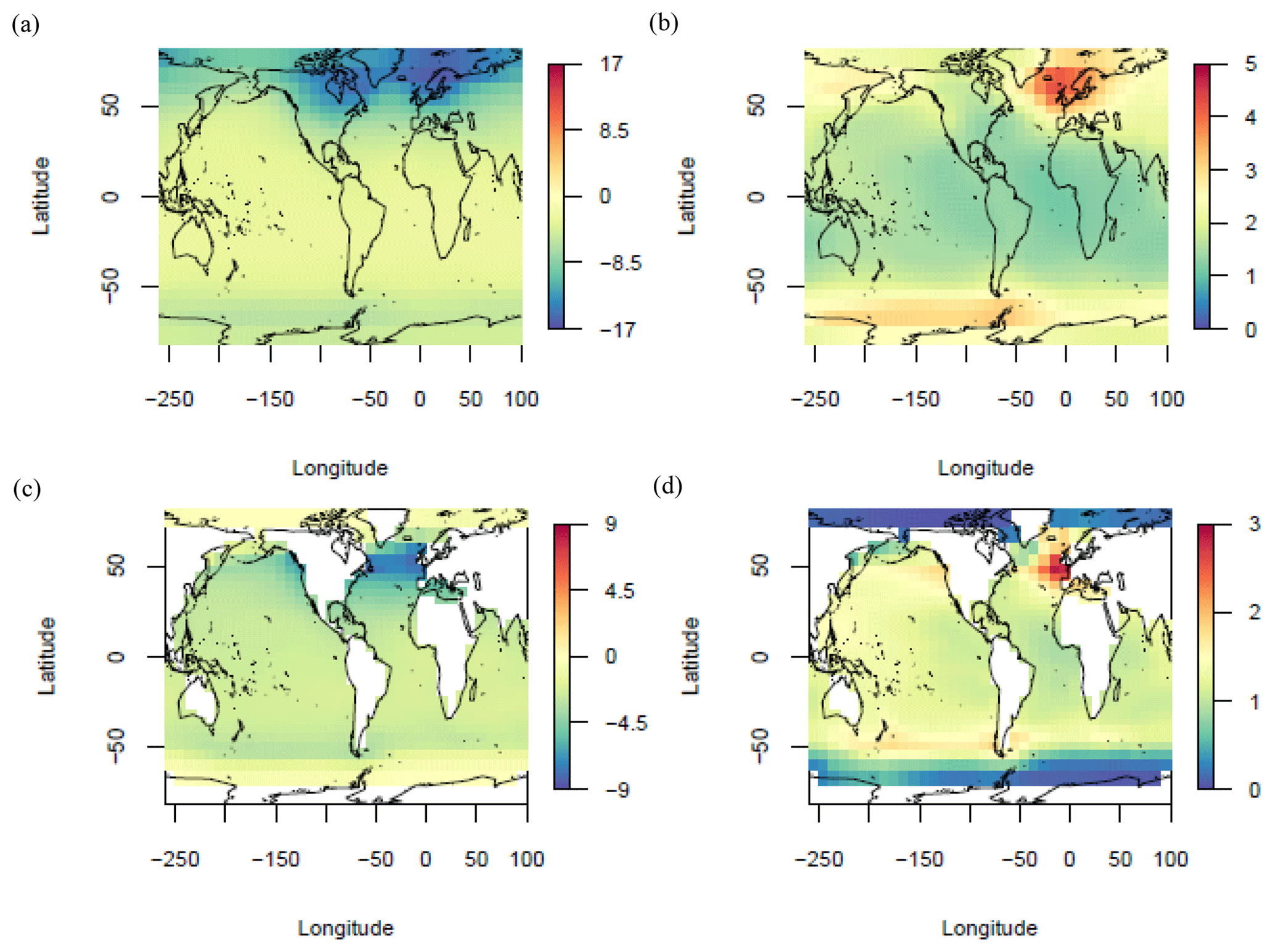
Figure 3 LGM change in surface air temperature (a–b) and sea surface temperature (c–d) (^∘C) ENS₁₀₄ mean (a, c) and standard deviation (b, d).

The ENS₁₀₄ mean ΔSAT and ΔSST spatial distributions are shown in Fig. 3. In line with observations (Annan and Hargreaves, 2013), the largest SAT decreases (>10 ^∘C) are simulated over the Laurentide and Eurasian ice sheets. The Equator-to-pole temperature gradient is also broadly reproduced. The largest SST decreases (≥4 ^∘C) are found in the North Atlantic and northeast Pacific, with more limited cooling ($\le -\mathrm{2}$ ^∘C) in the tropics and polar regions, again consistent with observations. However, the largest SST decreases ought to also be found in the Southern Hemisphere midlatitudes, whereas the simulated cooling is more moderate.

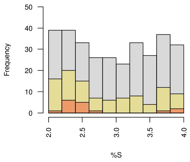
Salinity

The ENS₁₀₄ mean percentage increase in LGM salinity (and DIC, ALK, PO₄, etc.) due to decreasing sea level is 2.84±0.62 %S, and the range is 2 %S to 4 %S. There is no significant relationship between %S and ΔCO₂ in either ENS₁₀₄ or ENS₃₁₅, and the distribution of %S is similar in ENS₁₀₄ and in both ENS₃₁₅ and ENS₁₆ (Fig. 4).

Figure 4 Percentage increase in LGM salinity due to decreasing sea level distribution.

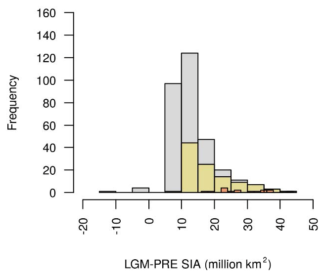
Sea ice

The ENS₁₀₄ mean LGM global annual sea ice area anomaly (ΔSIA) is 18.6±7.4 million km², and the range is 9.9 to 44 million km². There is a negative correlation between ΔSIA and ΔSAT ($r=-\mathrm{0.97}$) and between ΔSIA and ΔCO₂ ($r=-\mathrm{0.74}$). The negative correlation between ΔSIA and ΔCO₂ likely reflects the impact of changing atmospheric CO₂ on ΔSIA but may also include a smaller contribution from changing sea ice area to ΔCO₂. Increasing LGM sea ice area could, for instance, have capped the outgassing of CO₂ from the ocean, particularly in the Southern Ocean, and also reduced the net ocean–atmosphere CO₂ flux by decreasing the AMOC strength (see below). The negative correlation between ΔSIA and ΔSAT, and between ΔSIA and ΔCO₂, is reproduced in ENS₃₁₅ ($r=-\mathrm{0.96}$ and $r=-\mathrm{0.74}$, respectively). ΔSIA in ENS₁₀₄ also tends to be higher than in ENS₃₁₅ and smaller than in ENS₁₆ (Fig. 5).

Figure 5 LGM change in global sea ice area distribution.

As shown in Fig. 6, fractional sea ice cover increases in all regions where sea ice is present in pre-industrial simulations, although the largest increases take place in the North Atlantic.

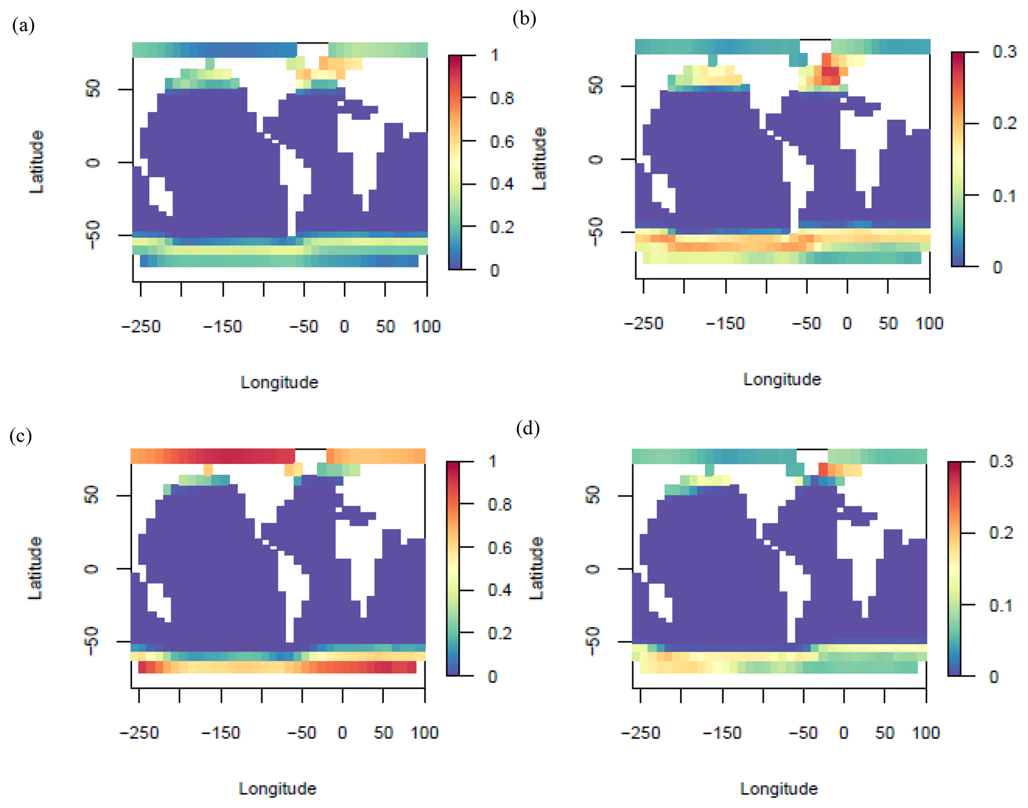
Figure 6 LGM-PRE (a–b) and PRE (c–d) fractional sea ice cover ENS₁₀₄ means (a, c) and standard deviations (b, d).

Precipitation

The ENS₁₀₄ mean spatial distribution of the LGM precipitation rate anomaly (ΔPP) is shown in Fig. 7. The LGM changes are mostly negative but regions of positive ΔPP do exist, notably over Siberia and Australia. The largest LGM precipitation decreases (>1.5 mm d⁻¹, with a maximum of 2.25 mm d⁻¹) are found over northern North America and from around the eastern North Atlantic to northwest Asia, coinciding with the location of the Laurentide and Eurasian ice sheets (and the largest increases in fractional sea ice cover), respectively. Relatively large precipitation decreases (>0.75 mm d⁻¹) are also simulated in eastern Asia, equatorial Africa and other regions of enhanced fractional sea ice cover. Comparison against a pollen-based precipitation reconstruction (Bartlein et al., 2011; Alder and Hostetler, 2015) suggest that the simulated precipitation changes over Europe and equatorial Africa are of the right direction, while precipitation changes over western Siberia at least ought to be negative. The sign of the precipitation changes over North America is mostly consistent with observations, which record negative changes over most of the continent. However, positive changes, which are also observed, are not captured. Although not shown here, comparison of the ENS₁₀₄ mean against the ENS₃₁₅ mean suggests that the precipitation patterns in the two are very similar, but the decreases generally tend to be higher in the ENS₁₀₄ mean. The precipitation decreases in ENS₁₀₄ conversely tend to be smaller than in ENS₁₆.

Figure 7 LGM change in precipitation rate (mm d⁻¹) ENS₁₀₄ mean (a) and standard deviation (b).

Ocean circulation

The ENS₁₀₄ mean LGM AMOC strength anomaly (Δψ_max) is $-\mathrm{2.8}\pm \mathrm{2.8}$ Sv, and the range is −8 to 4.7 Sv (Fig. 8). These estimates lie at the low end of the Δψ_max predicted by nine Paleoclimate Modelling Intercomparison Project phase 2 (PMIP2) (Weber et al., 2007) and eight PMIP3 (Muglia and Schmittner, 2015) coupled model simulations. However, they do not include the more negative Δψ_max predicted by Völker and Köhler (2013), for instance. The ENS₁₀₄ mean LGM-PRE AABW cell strength in the Atlantic Ocean (Δψ_min) is 0.1±1.2 Sv. A positive Δψ_min represents an LGM decrease in cell strength as we keep the original (negative) sign for anticlockwise flow of Antarctic water. A negative Δψ_min conversely represents an LGM increase in cell strength. However, the difference between the LGM and PRE Atlantic AABW here is not statistically significant. The range of Δψ_min is −4.3 to 4.3 Sv, roughly comparable to the range of Δψ_min predicted in Weber et al. (2007) (see also Muglia and Schmittner, 2015) but excluding the much larger ψ_min increase predicted by Kim et al. (2003), for example. As shown in Fig. 9, the northern limit of the ENS₁₀₄ mean LGM AABW cell is roughly at the same latitude as in the pre-industrial simulations. The maximum depth reached by the ensemble mean AMOC base is also similar to pre-industrial. Observations (Lynch-Stieglitz et al., 2007; Lippold et al., 2012; Gebbie, 2014; Böhm et al., 2015), conversely, suggest that the LGM AMOC shoaled to less than 2 km, raising its base depth by 2500 and 600 m at the north and south ends of the return flow, respectively. The LGM AABW, in turn, is thought to have filled the deep Atlantic below 2 km, reaching as far north as 65^∘ N, which is approximately 25^∘ north of its modern northern limit (Oppo et al., 2015).

Figure 8 LGM change in ψ_max and ψ_min (a–b) distributions.

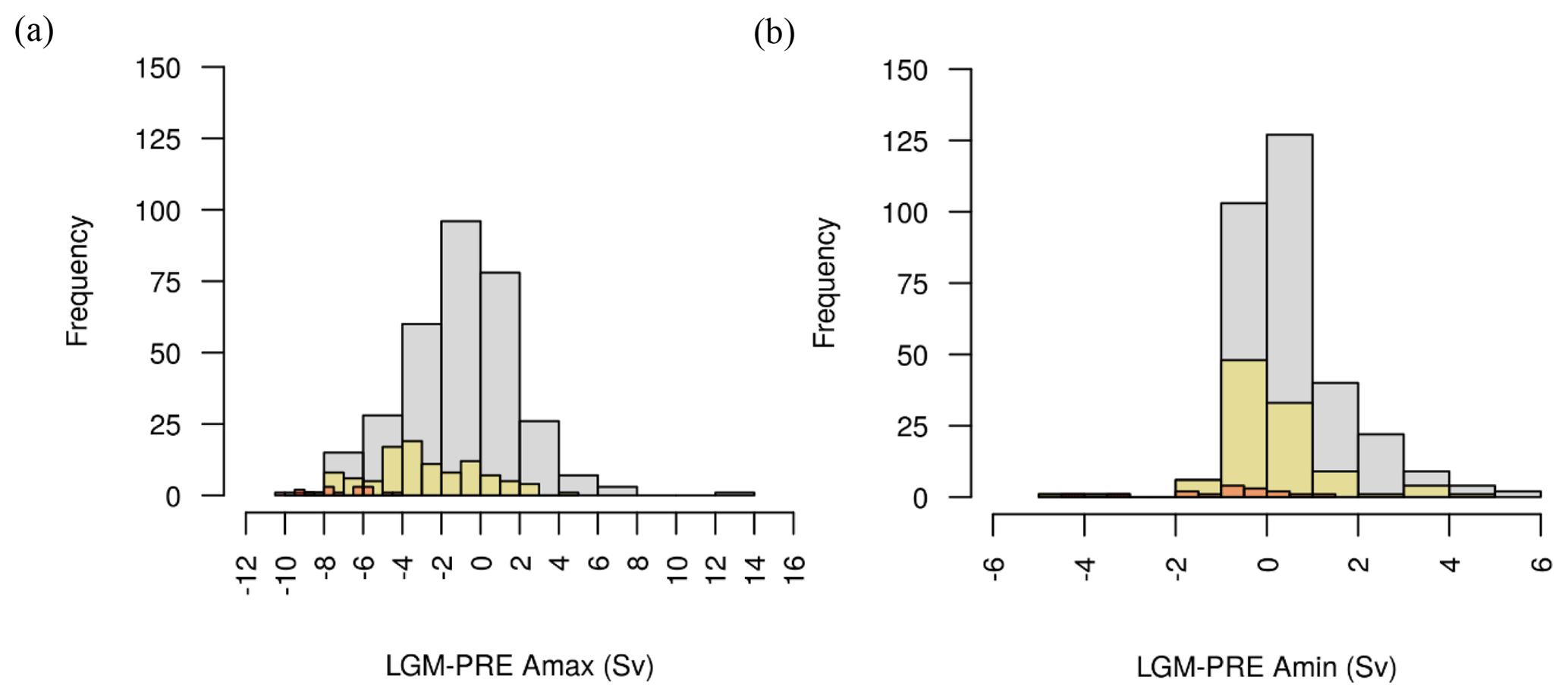
Figure 9 LGM (a–b) and PRE (c–d) Atlantic overturning stream function (Sv) ENS₁₀₄ means (a, c) and standard deviations (b, d).

Although not shown here, the ENS₁₆ ensemble members tend to exhibit a shoaling of the AMOC and enhanced penetration of AABW. With regard to Δψ_max and Δψ_min, one can see from Fig. 8 that these tend to be more negative (i.e. weaker AMOC and stronger AABW) than in ENS₁₀₄. The Δψ_max and Δψ_min in ENS₃₁₅ tend to conversely be more positive. In ENS₁₀₄, we also find a positive relationship between Δψ_max and ΔCO₂ (r=0.57) and a negative relationship between Δψ_min and ΔCO₂ ($r=-\mathrm{0.42}$). The relationships are reproduced in ENS₃₁₅ (r=0.59 and $r=-\mathrm{0.36}$, respectively). We additionally find, in both ENS₁₀₄ and ENS₃₁₅, negative correlations between Δψ_max and Δψ_min ($r=-\mathrm{0.62}$ and −0.63), Δψ_min and ΔSAT ($r=-\mathrm{0.4}$ and −0.4), and Δψ_max and ΔSIA ($r=-\mathrm{0.62}$ and −0.66), as well as positive correlations between Δψ_max and ΔSAT (r=0.68 and 0.66), and Δψ_min and ΔSIA (r=0.37 and 0.42). Based on these relationships, we hypothesise that increasing LGM AABW strength led to an expansion of the AABW cell. The latter in turn restricted the AMOC to lower depths and reduced its overturning rate (e.g. Shin et al., 2003). The increase in AABW strength was likely driven by increases in sea ice enhancing brine rejection. Sea ice increases in the North Atlantic may have additionally weakened the AMOC cell by locally reducing deep convection.

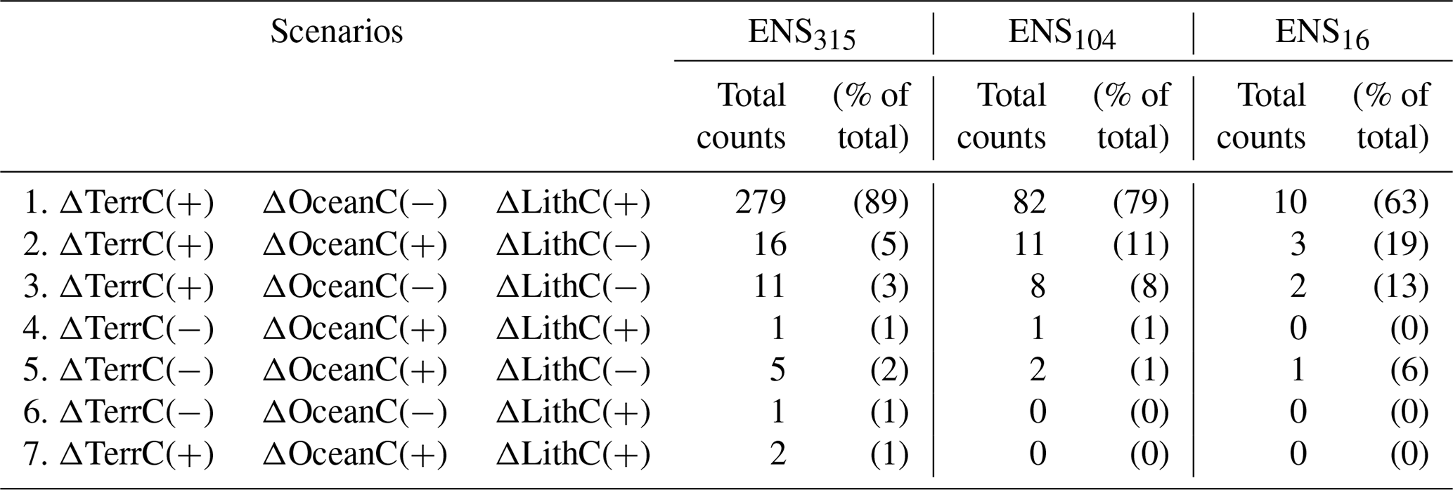
Table 3 LGM-PRE carbon partitioning scenarios in ENS₃₁₅, ENS₁₀₄ and ENS₁₆.

The relationships between Δψ_max, Δψ_min and ΔCO₂ are also consistent with increasing ψ_min (decreasing ψ_max) contributing to decreasing atmospheric CO₂. The replacement of North Atlantic Deep Water (NADW) by AABW in the North Atlantic would, for instance, have led to a dissolution of deep-sea sediment CaCO₃ due to AABW having a lower bottom water ${\mathrm{CO}}_{\mathrm{3}}^{\mathrm{2}-}$ concentration than NADW (see, e.g. Yu et al., 2014). The increased CaCO₃ dissolution flux would in turn have raised the whole ocean alkalinity, lowering the atmospheric CO₂. Enhanced AABW production would also have caused the deep ocean to become more stratified, allowing more DIC to accumulate at depth and promoting further CaCO₃ dissolution. A decrease in NADW formation could have additionally lowered atmospheric CO₂ by reducing CO₂ outgassing at the ocean surface and reducing the burial rate of deep-sea CaCO₃ due to the concomitant increase in deep-sea DIC accumulation. Further investigation is, however, required to confirm these causal relationships.

3.2.2 Terrestrial biosphere, ocean and lithospheric carbon

As shown in Fig. 10, most of the ensemble members in ENS₁₀₄ predict an LGM increase in terrestrial biosphere (ΔTerrC) and lithospheric¹ (ΔLithC) carbon inventory and a decrease in ocean carbon inventory (ΔOceanC). The remaining ensemble members predict one of four other scenarios of carbon partitioning, with the second most common scenario (11 % of ensemble members) being increasing terrestrial carbon and decreasing ocean and lithospheric carbon (Table 3). Similar patterns can also be observed in ENS₃₁₅ and ENS₁₆. A likely explanation for scenario 1 (increase in terrestrial biosphere and lithospheric carbon, decrease in ocean carbon) is that reduced soil decomposition (see below) causes a flux of CO₂ from the atmosphere to the land, leading to an immediate outgassing of CO₂ from the ocean to remove the atmospheric pCO₂ difference. The CO₂ outgassing also leads to an increase in surface [${\mathrm{CO}}_{\mathrm{3}}^{\mathrm{2}-}$] and subsequently deep ocean [${\mathrm{CO}}_{\mathrm{3}}^{\mathrm{2}-}$], which reduces CaCO₃ dissolution (and increases lithospheric carbon). The increase in CaCO₃ burial in turn decreases [${\mathrm{CO}}_{\mathrm{3}}^{\mathrm{2}-}$] and increases [CO₂], which is communicated back to the surface, with a resultant increase in atmospheric CO₂ (Kohfeld and Ridgwell, 2009). The above explanation is of course only part of the explanation for this dominant carbon partitioning scenario, with physical mechanisms also expected to play a role, in addition to any changes in ocean productivity and changes in land carbonate weathering (see below).

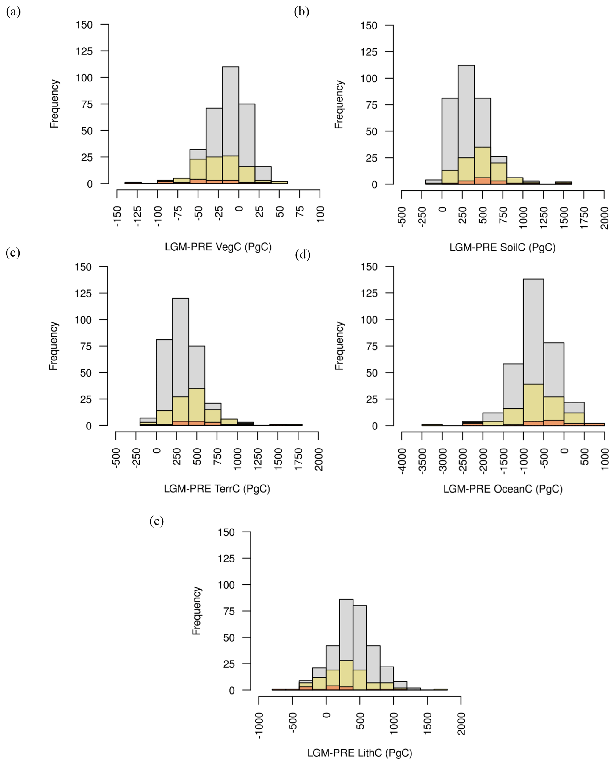
Figure 10 LGM change in vegetation (a), soil (b), terrestrial (vegetation plus soil) (c), ocean (d) and lithospheric (e) carbon inventory distributions.

The ENS₁₀₄ mean ΔTerrC, ΔOceanC and ΔLithC, the signs of which are consistent with scenario 1, are reported in Table 4, alongside previous estimates from observational data- and model-based studies. From here, we can see that the mean ΔTerrC is only aligned with a handful of estimates and no studies so far report a negative ΔOceanC. Instead, ΔOceanC is estimated to be positive, primarily based on carbon isotope data. The loss of hundreds of petagrams of carbon from the ocean in response to terrestrial carbon growth has, however, been previously proposed (e.g. Zimov et al., 2006). Moreover, if we assume that 90 % of the atmospheric CO₂ perturbation caused by the increase in terrestrial biosphere carbon reported in Table 4 gets removed by the ocean and sediments, the change in ocean carbon would be negative, even after adding the remaining carbon to be lost from the atmosphere to the ocean. We discuss what these results would likely mean for carbon isotope data in Sect. 3.2.6.

Table 4 LGM-PI difference in terrestrial (ΔTerrC), ocean (ΔOceanC) and lithospheric (ΔLithC) carbon inventory (PgC) in this study (ENS₁₀₄ mean, standard deviation and range) and previous studies. CR95 is Crowley (1995), AF98 is Adams and Faure (1998), Z03 is Zeng (2003), ZI09 is Zimov et al. (2009), PR11 is Prentice et al. (2011), ZE11 is Zech et al. (2011), BR12 is Brovkin et al. (2012), CI12 is Ciais et al. (2012), GL13 is Goodwin and Lauderdale (2013), OA13 is O'ishi and Abe-Ouchi (2013), SA is Sarnthein et al. (2013), PE14 is Peterson et al. (2014), AL15 is Allen et al. (2015), BG15 is Brovkin and Ganopolski (2015), SK15 is Skinner et al. (2015), SS16 is Schmittner and Somes (2016), ME17 is Menviel et al. (2017) and JE18 is Jeltsch-Thömmes et al. (2019).

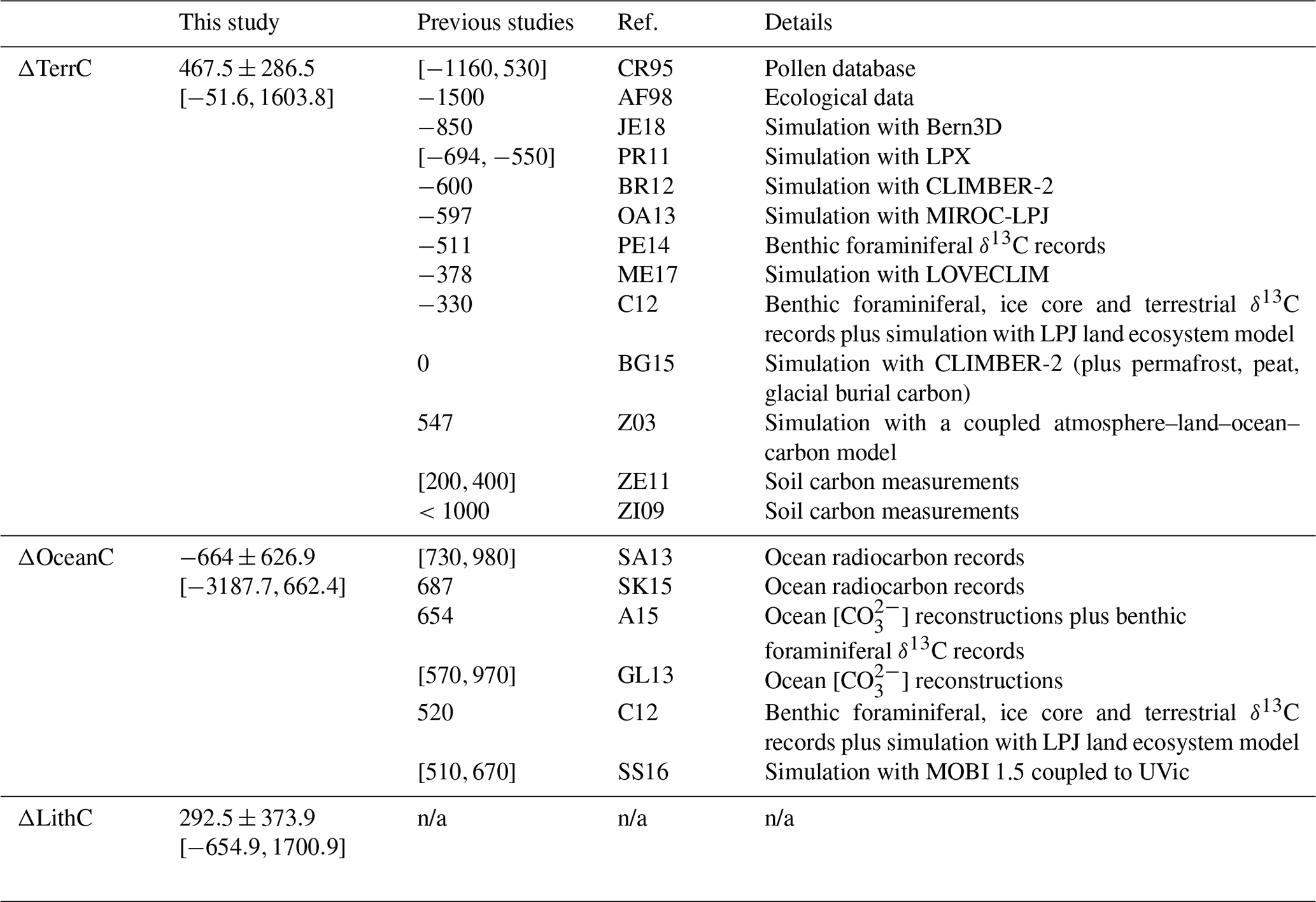
The positive ΔTerrC studies in Table 4 attribute the increase in terrestrial carbon to different factors: Zimov et al. (2009) and Zech et al. (2011) predict large increases in permafrost carbon, while Zeng (2003) ignores permafrost. Instead, the author attributes the glacial terrestrial carbon increase to the preservation rather than destruction of carbon in areas to be covered by the LGM ice sheets, lower soil respiration rates (in the active carbon pool) caused by a colder climate, as well as storage of carbon on exposed continental shelves. Here, neither the latter carbon accumulation mechanism, nor that of permafrost growth, are included. However, our model does attempt to capture the very slow rates of soil decomposition characteristic of permafrost (Williamson et al., 2006). We attribute the terrestrial carbon increase in our ensemble to a higher soil carbon inventory caused by a decreasing soil respiration rate. As can be seen from Fig. 10, vegetation carbon tends to conversely decrease at the LGM. As in Zeng (2003), we also do not assume that, as the ice sheets expand over terrestrial carbon, they destroy it. The lack of this potential loss term means that our ΔTerrC estimates may be higher than in many previous studies, irrespective of what the response of the terrestrial biosphere is to the LGM climate and CO₂ forcings. O'ishi and Abe-Ouchi (2011), for instance, estimated that the LGM climate is responsible for the loss of 502 PgC of terrestrial carbon, while another 388 PgC is removed by the ice sheets. Zeng (2003) conversely proposed that 431 PgC is preserved under the ice sheets at the LGM. This number includes 315 PgC present during the interglacial and another 116 PgC accumulated in response to the glacial climate forcings, prior to insulation of the terrestrial carbon from the atmosphere by the ice sheet coverage. Here, analysis of ENS₁₆ suggests that during the 1000 years of LGM ice sheet build-up, the terrestrial carbon inventory in the areas to be occupied by the ice sheets increases by between 6 and 444 PgC, yielding LGM “ice sheet or burial” carbon inventories between 318 and 1341 PgC (Table 5). This increase accounts for less than half of the total LGM change in terrestrial carbon (i.e. ΔTerrC) in the majority of simulations. However, if this burial carbon were to have been destroyed rather than preserved, ΔTerrC would be negative in all but three simulations, as opposed to positive in all but one simulation (Table 5).

Table 5 Ice sheet and non-ice-sheet terrestrial carbon stocks in ENS₁₆. Columns 2 and 5 show the amount of carbon stored in areas covered by the Eurasian and Laurentide ice sheets (“ice sheet”) during the pre-industrial and LGM periods, respectively. Column 3 is the difference between the two inventories. Column 4 is the LGM change in carbon in ice sheet areas expressed as a percentage of the total LGM terrestrial carbon change. Column 6 is the LGM change in carbon outside of the ice sheets.

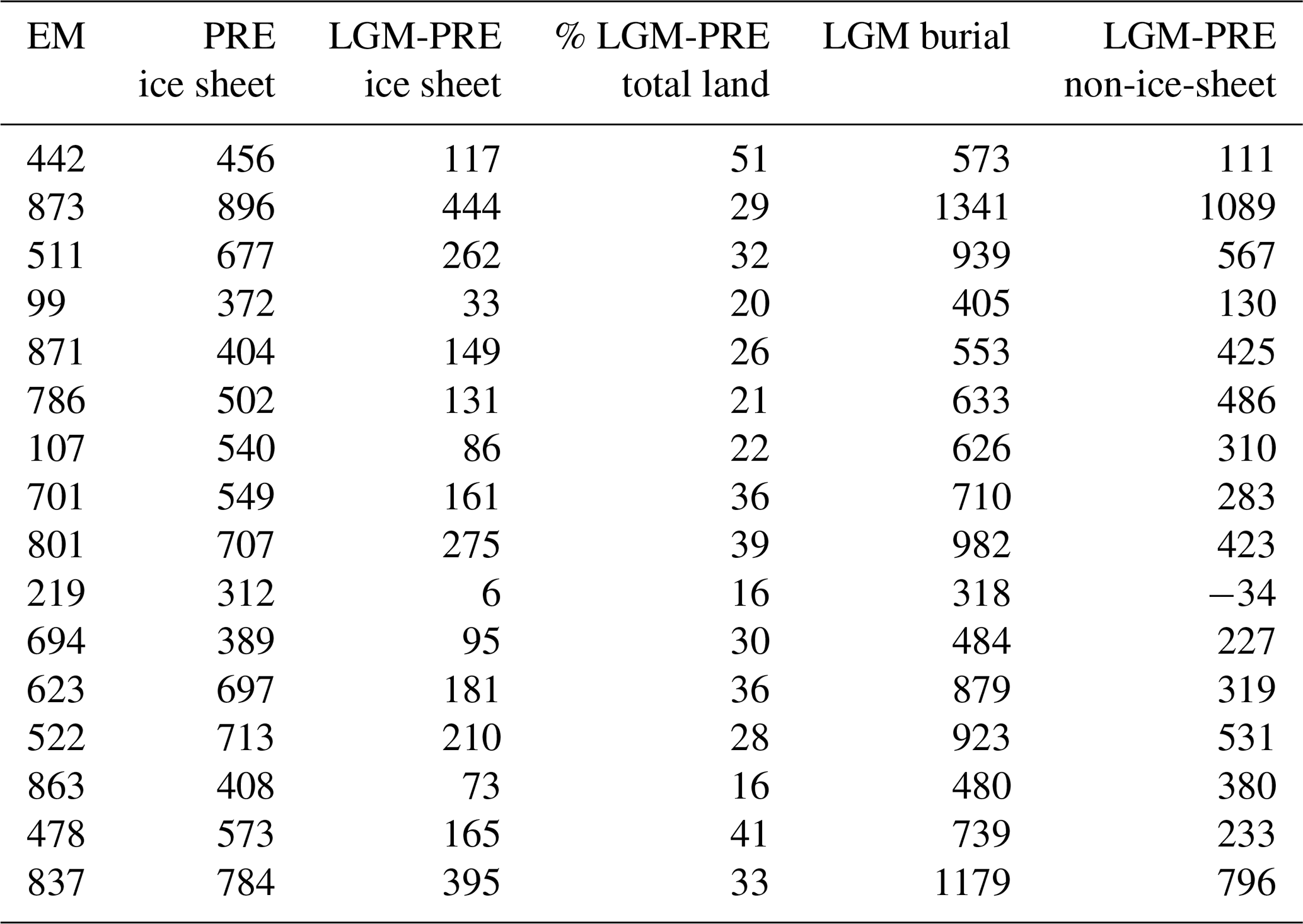
Most of the terrestrial carbon increase in areas to be covered by the ice sheets in ENS₁₆ is due to soil carbon, with vegetation carbon decreasing in all but one simulation. The range of terrestrial carbon increases and the associated burial carbon amounts include Zeng (2003)'s estimates. Our LGM burial carbon estimates would also accommodate an additional 250–550 PgC (Franzen, 1994) from increased glacial peat accumulation (Zeng, 2003). No observational data-based estimates of the LGM burial carbon inventory are available since only limited evidence exists for organic material being preserved by ice during glaciations (Franzen, 1994, and references in Weitemeyer and Buffett, 2006). Outside of the ice sheets, increases in the terrestrial carbon inventory in ENS₁₆ are mostly due to soil carbon, which increases in all simulations. Vegetation carbon, conversely, decreases in the majority of simulations. Our range of carbon changes outside of the ice sheet areas include the 198 PgC increase predicted by Zeng (2003) as a result of reduced soil respiration.

Although not evaluated directly, it is likely that similar ice sheet/non-ice-sheet terrestrial carbon proportions than in ENS₁₆ are found in ENS₁₀₄ and ENS₃₁₅ because of the similar climate change distributions in all three instances (see earlier sections). Although not shown here, the spatial distribution of ΔTerrC in ENS₁₆ is also similar to that of the ENS₁₀₄ (and ENS₃₁₅) mean. The spatial distribution of ΔTerrC in ENS₁₀₄ is shown in Fig. 11.

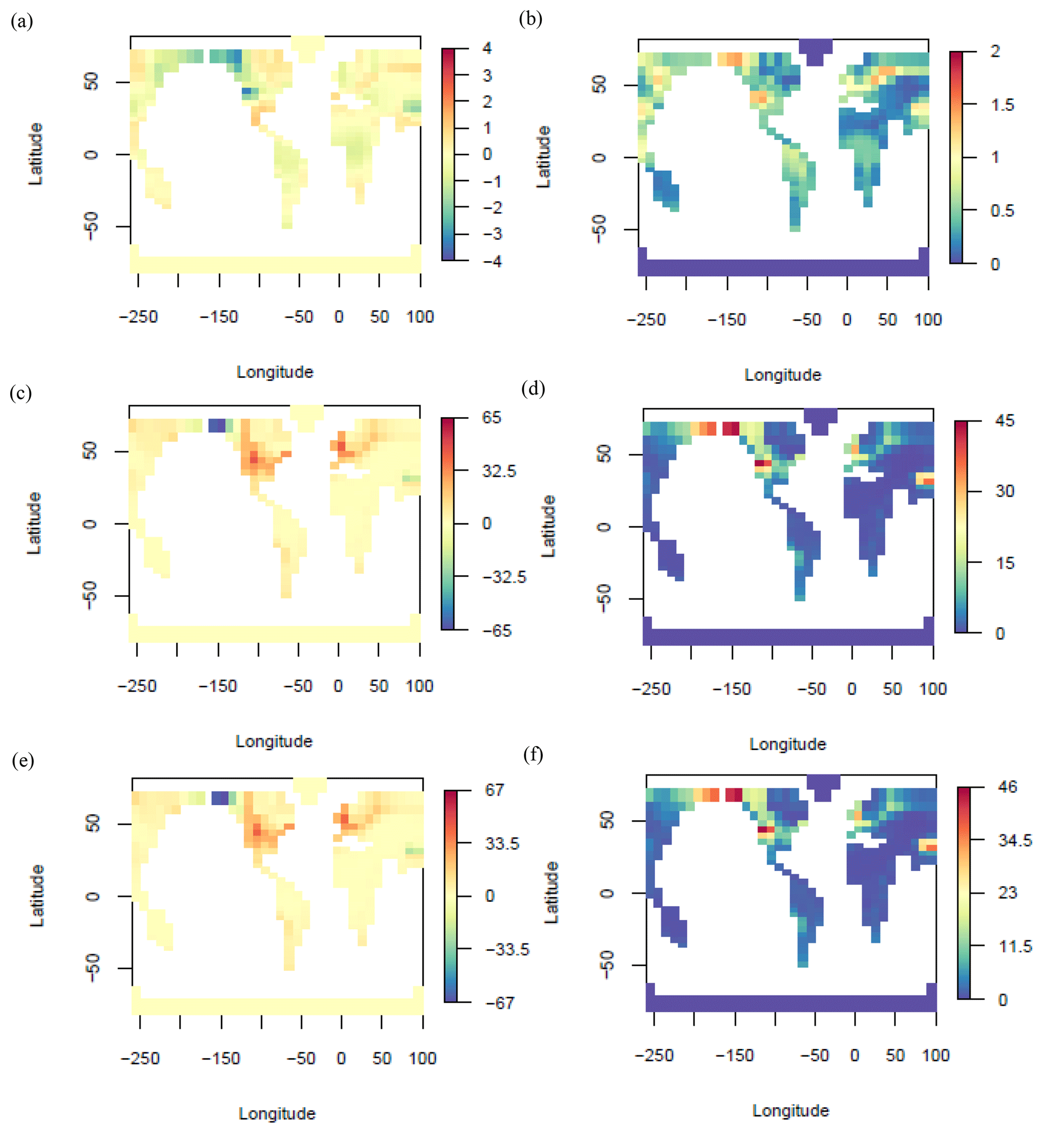
Figure 11 LGM vegetation (a–b), soil (c–d) and total terrestrial carbon changes (e–f) ENS₁₀₄ mean (a, c) and standard deviation (b, d). Units are kgC m⁻².

The largest increases in terrestrial carbon (≥20 kgC m⁻²) are found in North America and Europe/western Asia, both within and south of the Laurentide and Eurasian ice sheet margins (Fig. 11). Regions with smaller but still relatively large (≥10 kgC m⁻²) increases include the Andes and Patagonia regions, the southern tip of the African continent, eastern north Siberia and the grid cells just south of the Tibetan Plateau. The largest LGM decreases in terrestrial carbon (≥10 kgC m⁻²) conversely tend to be found in northwest North America, Beringia and the Tibetan Plateau region. Other regions with relatively large (≥5 kgC m⁻²) decreases include equatorial Africa and the deserts in central Asia. Everywhere else the LGM terrestrial carbon density increases by between 0 and 10 kgC m⁻². Comparison against paleoecological reconstruction studies (Crowley, 1995) suggests that the simulated terrestrial carbon changes within the Laurentide and Eurasian ice sheet areas are of the wrong sign, except in northwest North America, since these studies assume the complete destruction of vegetation and soils in ice sheet areas. Discrepancies between the ENS₁₀₄ and observations further arise from the rainforest regions, where the ensemble mean predicts terrestrial biosphere carbon density changes between −5 and 10 kgC m⁻², well above observed changes of $\sim -\mathrm{23}$ kgC m⁻². It is important to note, however, that as suggested in Zeng (2007), the rate of decomposition of soil carbon at the LGM may have been slower than assumed in pollen data-based studies. The largest increases in terrestrial carbon density (∼40 kgC m⁻²) produced by the ensemble mean are comparable to those found in areas with permafrost growth (Zimov et al., 2006). However, the peaks are potentially misplaced, being located within and south of the Laurentide and Eurasian ice sheet covered areas, rather than in eastern Siberia and Alaska. Alternatively, terrestrial carbon increases in eastern Siberia and Alaska are simply underestimated in the ensemble mean and large increases in terrestrial carbon indeed took place within the ice sheet areas during glacial periods.

The large LGM decreases in terrestrial carbon in northwest North America and adjacent Beringia are likely caused by precipitation decreasing comparatively more than SAT and causing the decrease in photosynthesis to exceed the decrease in soil respiration. However, it is also noteworthy that, although not shown here, the regions with the largest decreases in terrestrial carbon density, namely northwest North America, Beringia and the Tibetan Plateau area, are also the regions with the largest terrestrial carbon densities in the pre-industrial ENS₃₁₅ mean. We further note that the Tibetan soil carbon peak is overestimated in the latter, and the North American soil carbon peak misplaced, compared to observations. We attribute the first discrepancy to the lack of soil weathering in the model and the inclusion of land use effects in the observational data-based estimate (Holden et al., 2013b; Williamson et al., 2006). The second discrepancy is attributed to the lack of explicit representation of permafrost and the absence of moisture control on soil respiration (Williamson et al., 2006).

3.2.3 Ocean primary productivity

The ENS₁₀₄ mean LGM total POC export flux anomaly (ΔPOC_exp) is $-\mathrm{0.19}\pm \mathrm{1}$ PgC yr⁻¹ and the range is −2.57 to 2.56 PgC yr⁻¹, roughly consistent with previous model-based estimates (e.g. Brovkin et al., 2002, 2007; Bopp et al., 2003; Chikamoto et al., 2012; Palastanga et al., 2013; Schmittner and Somes, 2016; Buchanan et al., 2016). As shown in Fig. 12, compared to ENS₁₀₄, the POC flux decreases in ENS₃₁₅ and ENS₁₆ tend to be smaller and larger, respectively. ΔPOC_exp is positively correlated with Δψ_max (r=0.72 and 0.79) and negatively correlated with Δψ_min ($r=-\mathrm{0.62}$ and −0.58) in both ENS₁₀₄ and ENS₃₁₅. The correlations potentially suggest that decreasing AMOC strength and increasing AABW production led to decreasing POC export. One possible mechanism is enhanced deep ocean stratification due to increasing AABW formation leading to not only more efficient trapping of DIC at depth (see above) but also nutrients and therefore reduced availability in the euphotic zone. All else held constant, a weaker and shallower AMOC cell would also inhibit the transfer of nutrients from the deep ocean to the surface. A negative correlation can additionally be found between ΔPOC_exp and ΔSIA ($r=-\mathrm{0.55}$ and −0.6), probably because no primary production occurs beneath the sea ice surface. Increasing sea ice area at the LGM therefore leads to decreasing POC export flux. This would also explain the largest ENS₁₀₄ mean decreases in POC export flux, shown in Fig. 13, coinciding with increases in sea ice fraction.

Figure 12 LGM change in POC export flux distributions.

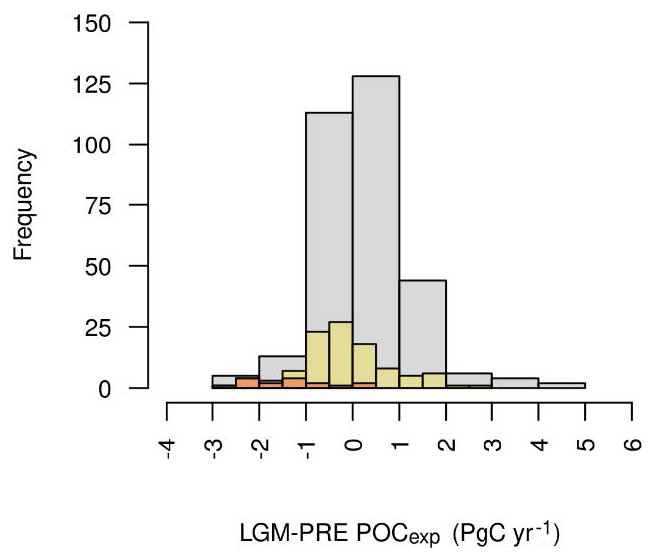
Figure 13 LGM surface POC export flux change (molC m⁻² yr⁻¹) ENS₁₀₄ mean (a) and standard deviation (b).

The largest ENS₁₀₄ LGM increases in POC export flux conversely occur at around 50^∘ S, roughly in front of the Antarctic sea ice margins. Increases in POC export are also simulated close to the North Pacific and Atlantic sea ice margins, as well as in the eastern equatorial Pacific and the southwest Atlantic upwelling region. The increases in POC export flux at the sea ice margins are likely caused by the advection of unutilised nutrients from underneath the sea ice. However, they may additionally be due to the enhanced iron availability from the increased supply of aeolian dust, particularly in the Southern Ocean and North Pacific since these are strongly limited by iron (Ridgwell et al., 2007). Iron fertilisation may also explain the increases in POC export flux in the eastern equatorial Pacific and in the southwest Atlantic upwelling region. Comparison against observations suggests that the ensemble mean POC flux changes immediately north, and south of the Antarctic sea ice margins align with observations of increased and reduced marine productivity in the subantarctic (∼45 to 60^∘ N) and Southern Ocean, respectively (Kohfeld, 2005; Kohfeld et al., 2013; Jaccard et al., 2013; Martínez-García et al., 2014). The simulated decreases in export flux in the Arctic and subarctic Atlantic (i.e. above approximately 50^∘ N), and the increases in export flux immediately south of 50^∘ N are also in agreement with previous reconstructions (Kohfeld, 2005; Radi and de Vernal, 2008). The mostly lower LGM export fluxes at the Equator and in the South Atlantic are conversely inconsistent with the observational data of Kohfeld (2005). The decreases may be caused by the increases in productivity in high-nutrient, low-chlorophyll (HNLC) regions reducing the phosphate (the other limiting nutrient in GENIE-1 besides iron) availability for photosynthesis in other regions. They may additionally be due to the model not simulating enhanced nutrient inventories in response to enhanced weathering or reduced shallower water deposition of organic matter. The model also does not vary wind speed, which may have resulted in stronger tropical upwelling in the Atlantic at the LGM. The evidence is more ambiguous (or missing) for the Pacific (Jaccard et al., 2010; Kohfeld and Chase, 2011; Kohfeld, 2005; Costa et al., 2016) and Indian oceans (Kohfeld, 2005; Singh et al., 2011) and is therefore not discussed in more detail here.

Figure 14 Land-to-ocean bicarbonate flux scaling factor (GWS) distributions.

3.2.4 Carbonate weathering and shallow water deposition

The ENS₁₀₄ mean land-to-ocean bicarbonate flux scaling factor (GWS) is 1.16±0.24 (corresponding to a percentage change in the land-to-ocean bicarbonate flux, %LOC, of 38.67), and the range is 0.52 to 1.5 (corresponding to a %LOC between −49.33 and 50). As shown in Fig. 14, the GWS in ENS₁₀₄ tends to be larger than in ENS₃₁₅ and smaller than in ENS₁₆. There is also a negative correlation between GWS and ΔCO₂ ($r=-\mathrm{0.52}$) in ENS₃₁₅, suggesting that increasing the input of bicarbonate to the ocean leads to a decrease in CO₂ by raising the inventories of ALK and DIC in a 2:1 ratio. In ENS₁₀₄, however, r is below the 0.05 significance level, suggesting that it is less important.

Figure 15 LGM change in deep-sea sediment CaCO₃ burial flux distributions.

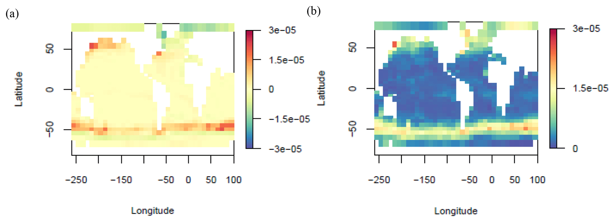
Figure 16 LGM deep-sea CaCO₃ burial rate change (mol cm⁻² yr⁻¹) ENS₁₀₄ mean (a) and standard deviation (b).

3.2.5 Deep-sea carbonate burial

The ENS₁₀₄ mean global deep-sea CaCO₃ burial flux anomaly ($\mathrm{\Delta }{\mathrm{CaCO}}_{{\mathrm{3}}_{\mathrm{bur}}}$) is 0.036±0.045 PgC yr⁻¹ and the range is −0.098 to 0.139 PgC yr⁻¹. The mean value is approximately 3 times larger than the observed value (Catubig et al., 1998), although the latter still falls within the range of simulated values. As shown in Fig. 15, $\mathrm{\Delta }{\mathrm{CaCO}}_{{\mathrm{3}}_{\mathrm{bur}}}$ in ENS₁₀₄ tends to be higher than in ENS₃₁₅ and lower than in ENS₁₆. The change in global deep-sea CaCO₃ burial flux anomaly is strongly determined by GWS, as suggested by the positive correlation (r=0.88 and 0.9) between the two, in both ENS₁₀₄ and ENS₃₁₅. Increasing %LOC (the percentage change in the land-to-ocean bicarbonate flux) should indeed enhance the CaCO₃ burial flux as increasing ALK means the deep ocean ${\mathrm{CO}}_{\mathrm{3}}^{\mathrm{2}-}$ will eventually increase. The latter in turn would cause the saturation horizon to fall, allowing CaCO₃ to accumulate over greater areas (which are now exposed to undersaturated waters) (Sigman and Boyle, 2000). The input of ALK to the surface ocean would also increase the rate of CaCO₃ export production (enhancing the sediment deposition flux of CaCO₃), since as discussed in Chikamoto et al. (2008), the latter is proportional to the production rate of POC (which is equal to the POC export flux), together with the sea surface saturation state with respect to CaCO₃, in GENIE-1. There is indeed also a positive correlation between %LOC and the global change in CaCO₃ export flux (r=0.27 and 0.4), and between the latter and $\mathrm{\Delta }{\mathrm{CaCO}}_{{\mathrm{3}}_{\mathrm{bur}}}$ (r=0.34 and 0.45) in both ENS₁₀₄ and ENS₃₁₅.

The ENS₁₀₄ mean spatial distribution of $\mathrm{\Delta }{\mathrm{CaCO}}_{{\mathrm{3}}_{\mathrm{bur}}}$ is shown in Fig. 16. Relatively large increases in burial flux ($\ge \mathrm{0.5}\times {\mathrm{10}}^{-\mathrm{5}}$ mol cm⁻² yr⁻¹) can be found at around 50^∘ S, in the North Pacific and to a lesser extent the North Atlantic. In other regions, the burial flux is significantly lower or negative, with the largest losses ($\le -\mathrm{0.5}\times {\mathrm{10}}^{-\mathrm{5}}$ mol cm⁻² yr⁻¹) occurring in the North Atlantic and arctic regions. The only exception is the western North Atlantic, which exhibits a large increase in burial. A comparison of the results against the reconstructions of Catubig et al. (1998) is somewhat difficult, as the coverage is poor but overall CaCO₃ burial was higher in the North Atlantic and the Pacific, and lower in the tropical and South Atlantic, and the Indian Ocean and Southern Ocean.

3.2.6 Other paleoproxies

As shown in Table 4, a frequent argument for a lower glacial terrestrial carbon inventory is the reconstructed mean glacial ocean δ¹³C value of approximately 0.35 ‰ lower than present due to the fact that plants discriminate against ¹³C during photosynthesis. In our simulations, conversely, it follows that the increase in glacial terrestrial carbon inventory would have resulted in an increase in ocean δ¹³C. Decreasing SSTs and increasing CaCO₃ weathering would have, moreover, likely raised it further (in the first instance, by enhancing fractionation at the air–sea interface, and in the second instance, through the input of isotopically heavy weathering products). However, as noted in Zeng (2007), the interpretation of the δ¹³C value can be complicated by factors such as the impact of enhanced glacial carbonate ion concentrations on δ¹³C in foramifera shells (Lea et al., 1999). In addition, there are other processes in our model which may have counteracted at least part of the increase in ocean δ¹³C. These include reduced marine productivity (e.g. Zimov et al., 2009), as phytoplankton discriminate against ¹³C during photosynthesis, giving the marine organic carbon reservoir a low δ¹³C. However, we note that the sign of this impact would additionally depend on the associated changes in organic matter remineralisation and burial. Another relevant process is greater sea ice area, which can lower the ocean δ¹³C by reducing the air–sea gas exchange and therefore the net transfer of ¹³C into the ocean (Stephen and Keeling, 2000). Moreover, we propose that adding missing processes could have decreased ocean δ¹³C even further. These include weaker surface winds (while in our model these are fixed), again through reduced air–sea gas exchange (Menviel et al., 2015), as well as enhanced weathering and reduced deposition of organic carbon at continental margins due to lower sea levels (Wallmann, 2014). Yet, further research is required here as one recent study suggests that taking into account these processes would most likely not (the possibility is not completely ruled out) allow reconciliation of a positive ΔTerrC with the observed mean glacial ocean δ¹³C value (Jeltsch-Thömmes et al., 2019).

Missing processes would likely also be needed to reconcile our lower POC export fluxes with deep ocean oxygen records. These records tend to indicate there was a decrease in LGM deep ocean oxygen concentration (Jaccard et al., 2016). Lower POC export fluxes would conversely have resulted in an increase in deep ocean oxygen due to reduced oxygen consumption at depth. When observed over sufficiently large areas, lower oxygen concentrations can support the presence of an enhanced ocean carbon inventory as deoxygenation can be explained by reduced ocean ventilation (the sole input of oxygen is from the ocean surface) (Wagner and Hendy, 2015). The reduced ventilation is, in turn, assumed to have led to the accumulation of a significant amount of DIC in the ocean interior. Thus, explaining the lower deep ocean oxygen concentrations without having to reduce ocean ventilation as extensively as suggested by previous studies would as a minimum likely require LGM export production to have increased rather than decreased. However, it may be possible to increase deep ocean oxygen consumption by increasing organic matter at depth but keeping the surface POC export flux constant. This would require adding missing processes such as increasing remineralisation depth with decreasing ocean temperature and increasing ballasting into our model (Kohfeld and Ridgwell, 2009; Menviel et al., 2012).

4 Conclusions

We have used an uncertainty-based approach to investigating the LGM atmospheric CO₂ drop by simulating it with a large ensemble of parameter sets and exploring the range of possible responses. Despite our ensemble varying many of the parameters thought to contribute to variability in glacial–interglacial atmospheric CO₂, we estimated that up to ∼ 60 ppmv of ΔCO₂ could be attributed to processes not included in our model and error in our process representations. As a result, we treated ΔCO₂ between $\sim -\mathrm{90}$ and −30 ppmv as equally plausible and focused on describing the responses of the subset of simulations with this ΔCO₂. We found the range of responses to be large, including the presence of five different ways of achieving a plausible ΔCO₂ in terms of the sign of individual carbon reservoir changes. However, several dominant changes could be detected. Namely, the LGM atmospheric CO₂ decrease tended to predominantly be associated with decreasing SSTs, increasing sea ice area, a weakening of the AMOC, a strengthening of the AABW cell in the Atlantic Ocean, a decreasing ocean biological productivity, an increasing CaCO₃ weathering flux and an increasing deep-sea CaCO₃ burial flux. The majority of our simulations also predicted an increase in terrestrial carbon, coupled with a decrease in ocean and an increase in lithospheric carbon. The increase in terrestrial carbon, which is uncommon in LGM simulations, was attributed to reduced soil respiration in response to the climate forcings, as well as our choice to preserve rather than destroy carbon that accumulates in ice sheet areas. The dominant changes were broadly in agreement with observations and paleoproxies other than carbon isotope and oxygen data, which we did not evaluate directly. However, we advise more detailed comparisons in future studies. It is also likely that our results can only be reconciled with carbon isotope and oxygen data if processes currently missing from our model are taken into account.

Appendix A: The OLR feedback parameter

The ensemble parameter OL1 is varied through all stages but stage 1. OL1 describes the unmodelled response of clouds to global average temperature change and corresponds to the K_LW1 constant in the equation below (Eq. 1 in Holden et al., 2010a):

$$\begin{array}{}\text{(A1)}& {\displaystyle }{L}_{\mathrm{out}}^{\ast }=L_{\mathrm{out}}(T,q)-K_{\mathrm{LW}\mathrm{0}}-K_{\mathrm{LW}\mathrm{1}}\mathrm{\Delta }T,\end{array}$$

where L_out(T,q) is the unmodified “clear skies” OLR term of Thompson and Warren (1982), K_LW0 is the clear-sky outgoing long-wave radiation parameter (OL0), representing the effects of clouds on the unmodified OLR (with K_LW0 only ever taking positive values), and ΔT corresponds to the difference between the globally averaged surface air temperature and the equilibrium pre-industrial temperature (Holden et al., 2010a).

In stage 1, OL1 is set to zero and T₀ can be set to any value. The temperatures simulated at the end of stage 1 are used to define T₀ in stage 2 and in the LGM simulations.