A spatiotemporal reconstruction of sea-surface temperatures in the North Atlantic during Dansgaard–Oeschger events 5–8

Here, we establish a spatiotemporal evolution of the sea-surface temperatures in the North Atlantic over Dansgaard–Oeschger (DO) events 5–8 (approximately 30–40 kyr) using the proxy surrogate reconstruction method. Proxy data suggest a large variability in North Atlantic sea-surface temperatures during the DO events of the last glacial period. However, proxy data availability is limited and cannot provide a full spatial picture of the oceanic changes. Therefore, we combine fully coupled, general circulation model simulations with planktic foraminifera based sea-surface temperature reconstructions to obtain a broader spatial picture of the ocean state during DO events 5–8. The resulting spatial sea-surface temperature patterns agree over a number of different general circulation models and simulations. We find that sea-surface temperature variability over the DO events is characterized by colder conditions in the subpolar North Atlantic during stadials than during interstadials, and the variability is linked to changes in the Atlantic Meridional Overturning circulation and in the sea-ice cover. Forced simulations are needed to capture the strength of the temperature variability and to reconstruct the variability in other climatic records not directly linked to the sea-surface temperature reconstructions. This is the first time the proxy surrogate reconstruction method has been applied to oceanic variability during MIS3. Our results remain robust, even when age uncertainties of proxy data, the number of available temperature reconstructions, and different climate models are considered. However, we also highlight shortcomings of the methodology that should be addressed in future implementations.

1 Introduction

The Dansgaard–Oeschger (DO) events of the last glacial are some of the most prominent climate variations known from the past. Ice cores from Greenland show multiple temperature excursions during the last glacial period as the climate over Greenland alternated between cold stadial (Greenland Stadial, GS) and warmer interstadial (Greenland Interstadial, GI) conditions during a period of roughly 1500 years (Grootes and Stuiver, 1997). Each DO event is characterized by an initial temperature rise of 10 ± 5 ^∘C toward GI conditions in a few decades, a more gradual cooling over the following several hundreds of years, and a relatively rapid temperature drop back to GS at the end of most of the events (Johnsen et al., 1992; Dansgaard et al., 1993; North Greenland Ice Core Project members, 2004; Kindler et al., 2014). DO events are manifested not only in Greenland but around the world. Concurrent with warm GIs, proxy records show a warmer and wetter climate in Europe, an intensified Asian summer monsoon, and a cooling of parts of the Southern Hemisphere (for overviews, see Voelker, 2002; Rahmstorf, 2002).

With its proximity to Greenland, much attention has been paid to the North Atlantic in reconstructing the millennial-scale GS/GI climate cycles. Reconstructions from the Marine Isotope Stage 3 (MIS3, 24–59 kyr ago), during which about 15 DO events occurred, suggest a large variability in sea-surface and subsurface temperatures in the North Atlantic coincident with the temperature variability in Greenland. Elliot et al. (2002) and Bond et al. (1993) show significant decreases in sea-surface temperatures (SSTs) in the North Atlantic during GSs. In the Nordic Seas, on the other hand, subsurface temperatures are found to increase during the same periods (Rasmussen and Thomsen, 2004; Dokken et al., 2013; Ezat et al., 2014). Large movements of the oceanic temperature fronts are associated with the variability (Voelker and de Abreu, 2013; Eynaud et al., 2009) and Rasmussen et al. (2016) recently suggested a gradual northward movement of warm subsurface waters during GSs compared to GIs in the North Atlantic. New studies also suggest variability in the sea-ice cover of the Nordic Seas with expanded sea-ice cover during GSs compared to GIs when the sea-ice cover retreated. These changes coincide with the temperature variability in Greenland (Dokken et al., 2013; Hoff et al., 2016). However, expanded sea-ice cover during GIs compared to GSs has also been suggested based on dinoflagellate cyst assemblages (Eynaud et al., 2002; Wary et al., 2016).

Several mechanisms involving the North Atlantic have been proposed to explain the GS/GI cycles. These include latitudinal shifts in the North Atlantic Deep Water formation site (Labeyrie et al., 1995; Ganopolski and Rahmstorf, 2001; Arzel et al., 2010; Colin de Verdiere and Raa, 2010; Curry et al., 2013; Sevellec and Fedorov, 2015); changes in the heat transport to the North Atlantic due to either internal instabilities in the Atlantic Meridional Overturning Circulation (AMOC; Broecker et al., 1990; Tziperman, 1997; Marotzke, 2000; Ganopolski and Rahmstorf, 2001) or a salt oscillator (Peltier and Vettoretti, 2014; Vettoretti and Peltier, 2016); and changes in the sea-ice cover of the Nordic Seas (Broecker, 2000; Gildor and Tziperman, 2003; Masson-Delmotte et al., 2005; Li et al., 2005; Dokken et al., 2013; Petersen et al., 2013). However, the mechanisms behind the DO events are still debated, and it is not clear whether the events are forced by internal ice sheet instabilities, or if they originate from variability within the ocean–atmosphere system or from a combination of both.

To understand the dynamics behind the DO events, integrating climate modeling and paleoreconstructions is necessary. While modeling studies can demonstrate feasibility of all of the abovementioned mechanisms for DO variability, proxy data should be used to assess the realism of such scenarios. However, due to limited proxy data and computing resources, model–data integration poses a challenge to the community. Although the North Atlantic region contains much information from the last glacial period, marine paleoclimatic reconstructions are still confined to suitable locations for coring, making the information sparse and spatially limited. In addition, the marine proxy records that cover MIS3 have variable temporal resolution, and even the best resolved marine reconstructions are of much lower resolution than the ice-core records from Greenland. Although there are a number of idealized attempts to simulate the full MIS3 period (e.g., Brandefelt et al., 2011; Van Meerbeeck et al., 2009; Peltier and Vettoretti, 2014), the lack of high-resolution coupled climate model simulations (including interactive ice sheets) is arguably another limiting factor for our understanding of the mechanisms behind DO events.

The model–data integration for the recent past has been performed using various techniques. One example is regression models that are based on the relationship between climate model variables or observations, and are applied (directly) to proxy reconstructions (e.g., Rahmstorf et al., 2015). While using regression models is computationally efficient, it inherently assumes the same linear relationships between variables in the past as for the present – an assumption which might not be true, especially when investigating a glacial climate. Regression models have also been applied using climate models with MIS3 boundary conditions (Zhang et al., 2015); however, linearity between the model variables is still assumed and this assumption may be invalid during the abrupt non-linear DO events. Another example is data assimilation and inversion techniques which are becoming more frequently used for paleoclimate studies. For example, Kurahashi-Nakamura et al. (2014) and Gebbie et al. (2015) have used these techniques to investigate the ocean circulation during the Last Glacial Maximum (LGM). However, due to the lack of proxy data, these studies often focus on reconstructing a relatively stable climate state, which allows for aggregating a large number of proxy records over a long time span. While data assimilation would be an ideal method for confining model simulations, it is not feasible in the transient case of MIS3 where the proxy data coverage is very sparse. Due to their individual restrictions, both regression methods as well as data assimilation, together with long coupled climate model simulations, appear suboptimal for studying the non-linear changes over the long time period of MIS3.

In this study, we combine the physically consistent output of model simulations with the temporally accurate information from proxy data in the North Atlantic and the Nordic Seas by applying the proxy surrogate reconstruction (PSR) method. This method has recently undergone sensitivity tests and has been successfully applied in reconstructing European atmospheric temperatures over the last 200 years (Franke et al., 2011) and the observed global decadal temperature variability of the last century (Gómez-Navarro et al., 2017). Although Graham et al. (2007) used one coastal SST reconstruction together with terrestrial records to reconstruct US climate back to 500 AD, the PSR method has, to our knowledge, never been applied to ocean data before. Also, the PSR method has never before been used for the MIS3 time period. Here, we use the SST variability in the North Atlantic and the Nordic Seas during the last glacial period as a test case for the PSR method to see whether the method can widen our knowledge of spatial patterns back in time. In doing so, we also aim to learn about the underlying DO variability in the North Atlantic region.

We present the PSR method together with the proxy-based temperature reconstructions and model simulations in Sect. 2, test the method in Sect. 3, show the results of the method in Sect. 4, and discuss the results in Sect. 5.

2 Materials and methods

2.1 Proxy surrogate reconstruction

We use the PSR method which was first introduced by Graham et al. (2007) to combine sparse proxy data and spatially complete and physically consistent climate model output. In this way, we can produce a climate reconstruction that is complete in both space and time. A similar method using analogs was first introduced for weather forecasting by Lorenz (1969). Briefly, the PSR method is as follows. A low-pass filtered collection of years from one or several model simulations is treated as a pool of possible “climate states”. Then, for any time period in which we have a set of proxy data, we find the climate state from the model pool that best matches the proxy data: an “analog”. This is done using an objective cost function. By repeating this and finding analogs for all time steps in the proxy data, we compile a set of climate states from the model pool which is consistent with the proxy data. We thus have a time series of modeled climate states with a complete spatial coverage which is the best fit to the spatially sparse proxy data. Furthermore, since the model simulates variables other than those that are used in the matching, we can also reconstruct variables which are constrained by the variability of the proxy data and for which no paleoreconstruction exists.

We follow the PSR implementation introduced by Franke et al. (2011) and apply the method to SSTs. First, we find the one model grid cell that is closest to each proxy record location and extract the modeled temperature for each climate state from those locations. Results are not sensitive to this choice as picking the four closest grid cells yields nearly identical results. Second, we define a cost function for deciding which of the climate states will represent a given proxy time step. For this, we use the root mean square error (RMSE) in temperature space as a distance measure:

$$\begin{array}{}\text{(1)}& d(T^{\mathrm{p}},T^{\mathrm{m}})=\sqrt{{\displaystyle \frac{{\sum }_{i=\mathrm{1}}^I{w}_i(T_i^{\mathrm{p}}-T_i^{\mathrm{m}}{)}^{\mathrm{2}}}{I}}},\end{array}$$

where $T_i^{\mathrm{p}}$ and $T_i^{\mathrm{m}}$ are the proxy and model temperature anomaly records at location i, respectively. The anomalies are calculated from the temporal mean of the proxy data and each individual model simulation, respectively. I is the total number of core locations with a proxy-based reconstructed temperature value at the given time step, ranging between 12 and 14 in this study. w_i is a weight which one could apply to reduce the bias toward areas with large variability. However, we decided not to use any weight (w_i=1), because the spatial differences in interannual variability in the ocean are much smaller than spatial differences in monthly variability in the atmosphere (which is what motivated Franke et al., 2011 to use w_i). We did test several different weighting options; however, no weighting function impacted the final results, further justifying our choice of setting $w_i=\mathrm{1}.$

As a final step, we create a composite T^c consisting of several analogs: the model climate states with the smallest d. For a given time step, we choose to form the composite based on the 10 analogs (N=10) with the smallest RMSE and weight the analogs by a function of the RMSE:

$$\begin{array}{}\text{(2)}& T^{\mathrm{c}}(x,y,t=k)=\sum _{n=\mathrm{1}}^N{W}_n{T}_n^{\mathrm{m}}(x,y),\end{array}$$

where x and y are the two spatial dimensions, t is time dimension (on the proxy time axis), k marks a given year in the proxy record, n is a specific analog from the model pool, $T_n^{\mathrm{m}}$ is the model temperature field for analog n, and the weight scalar W_n is defined to be inversely proportional to the RMSE distance d_n:

$$\begin{array}{}\text{(3)}& W_n={\displaystyle \frac{\left(\sum _{n=\mathrm{1}}^N{d}_n\right)-d_n}{\sum _{n=\mathrm{1}}^N\left[\left(\sum _{n=\mathrm{1}}^N{d}_n\right)-d_n\right]}}.\end{array}$$

Note that because the sum of W is scaled to be 1, the composite is not very sensitive to the increase in number of analogs (N), as usually analogs beyond n=10 are assigned very small weights. The choice of number of analogs in the composite is further discussed in Sect. 3.2.1.

As we repeat this algorithm for each proxy time step, we construct a three-dimensional dataset of the composites: the surrogate reconstruction c_i. We either present the results as a surrogate time series or as composite maps of the surrogate reconstruction. The results are evaluated against the proxy records by comparing the RMSE, the standard deviation, and the correlation coefficient between the proxy records and the PSR over 30–40 kyr.

2.2 Proxy records

We compiled proxy-based SST reconstructions from 14 marine sediment cores located in the North Atlantic and the Nordic Seas for the time interval from 30 to 40 kyr (GS/GI cycles 5–8) (Table 1, Fig. 1). For 10 of the cores (Table 1), we recalculate SST estimates based on assemblage counts of planktic foraminifera and the maximum likelihood (ML) technique (ter Braak and Looman, 1986; ter Braak and Prentice, 1988; ter Braak and van Dam, 1989). We use the North Atlantic core-top calibration dataset developed within the MARGO framework (Kucera et al., 2005a, b). The calibration uses modern SST values for 10 m water depth during summer (July, August, September – JAS) taken from the World Ocean Atlas version 2 (WOA, 1998). Telford et al. (2013) showed that the temperature signal recorded by planktic foraminifera may not always originate from the very surface. The reason for this is that some foraminiferal species live in a depth range spanning several tenths of a meter of the upper ocean (Rebotim et al., 2017). However, Telford et al. (2013) showed that for cores north of 25^∘ N the reconstructions from different depths resemble one another. The cores used in our study are located north of 43^∘ N, and we therefore assume that any biases related to the chosen calibration depth are negligible for our reconstructed temperatures. The choice of transfer function is most often based on the RMSE between the measured and inferred variables, used to assess the predictive power of the transfer function. Choosing a transfer function with low RMSE will, in a statistical sense, provide the best transfer function model. The estimation of the predictive power of transfer functions assumes that the test sites are independent from the modeling sites. However, autocorrelation is common in ecological data. Using an independent dataset, Telford and Birks (2005) explored and quantified how autocorrelation affects the statistical performance of different transfer functions. They concluded that the true RMSE is approximately twice the value of previously published estimates for some methods, e.g., the modern analog technique. In this study, we have chosen the ML transfer function technique which is based on an unimodal species response. We base this decision on the results by Telford and Birks (2005) that suggest that this method, and other methods based on the assumption of an unimodal species–environment response model, is more robust with regards to spatial structure in the data. For the ML technique, the RMSE is 1.8 ^∘C, based on cross-validation using bootstrapping.

Dokken and Jansen (1999)Dokken et al. (2013)Dokken et al. (2013)Hagen and Hald (2002)Hagen and Hald (2002)Voelker (2018)Elliot et al. (1998)Barker et al. (2015)Barker et al. (2015)van Kreveld et al. (2000b)van Kreveld et al. (2000a)Hall et al. (2011b)Hall et al. (2011a)Weinelt et al. (2003)Weinelt et al. (2003)Peck et al. (2007)Peck et al. (2007)Obrochta et al. (2012)Bond et al. (1999)Sánchez Goñi et al. (2008)Sánchez Goñi et al. (2008)(Bard et al., 2004)Kiefer (1998)Kiefer (1998)Salgueiro et al. (2010b)Salgueiro et al. (2010a)Labeyrie et al. (1999)Labeyrie et al. (1999)Waelbroeck et al. (2001)

Table 1 Core sites and age model information.

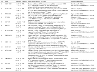
Conversion of GISP2 ages to equivalent GICC05 ages is done according to the NGRIP-GRIP-GISP2 match points in Seierstad et al. (2014). Ages for respective North Atlantic Ash Zones (NAAZs) and Faroe Marine Ash Zones (FMAZs) are according to Davies et al. (2012). NGRIP is the North Greenland Ice Core Project. IRD is ice-rafted debris. SST estimates are either based on assemblage counts of planktic foraminifera and the ML technique or on records of the percentage of the planktic foraminifera Neogloboquadrina pachyderma (%NP).

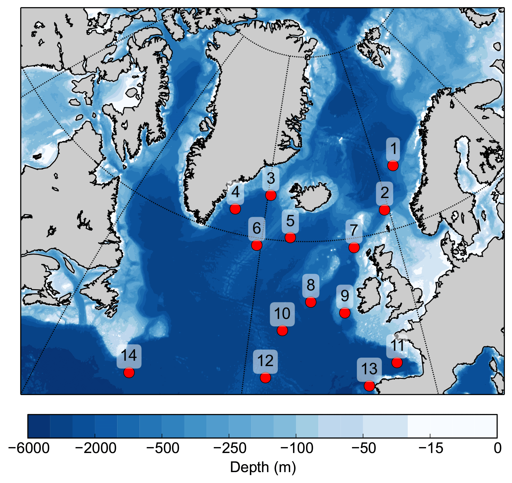
Figure 1 Core locations of the proxy data; numbers correspond to Table 1. Colors indicate bathymetry.

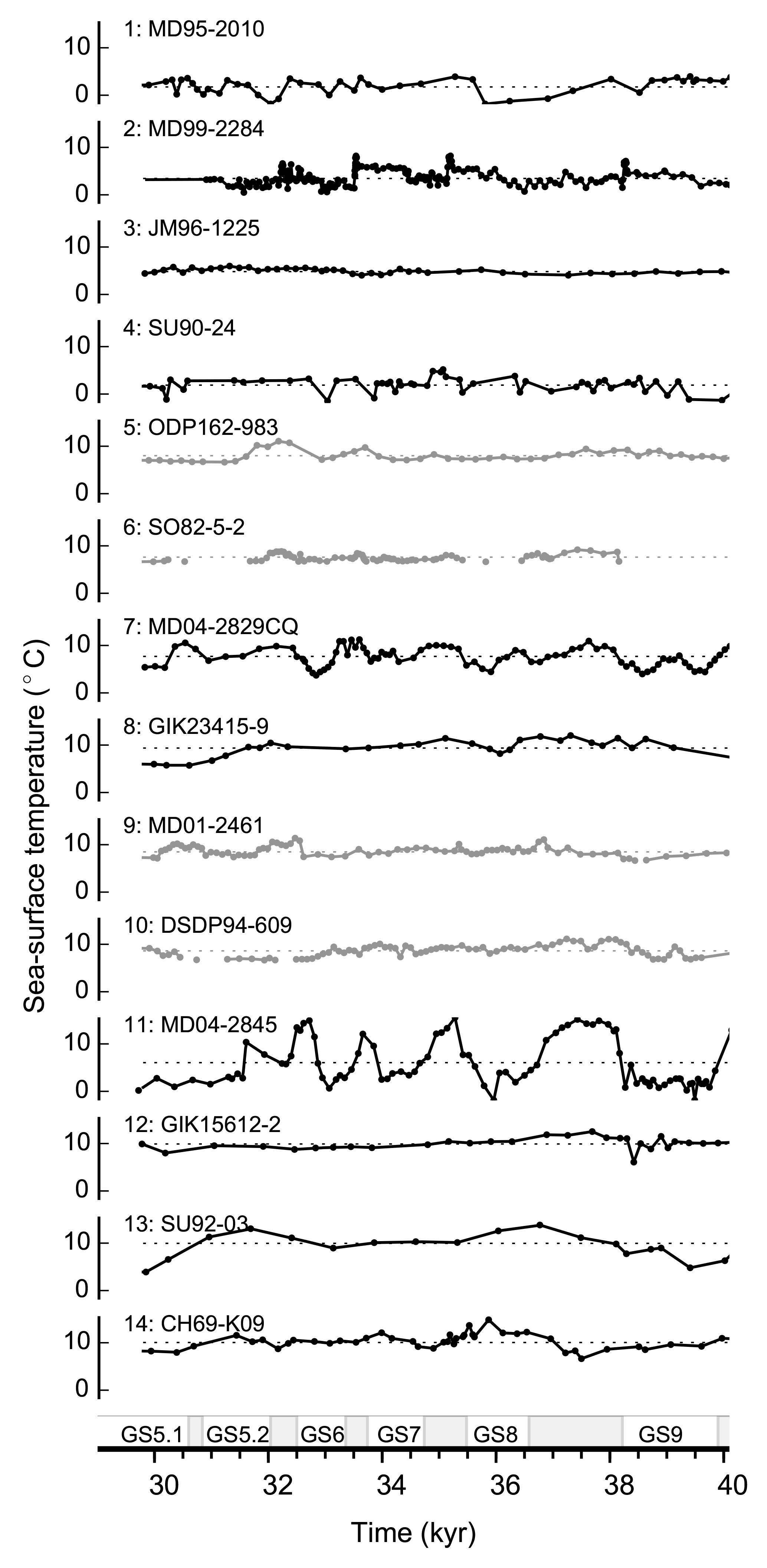
Figure 2 The proxy data. Black time series correspond to ML SSTs while grey time series are produced with %NP. Dots mark a data point, and stippled lines mark the mean of the proxy record over the given time period. Shaded grey areas on x axis mark the GIs, while the GSs are named.

For the remaining four cores, from which full planktic foraminifera assemblage counts are not available, we use records of the percentage of the polar planktic foraminifera Neogloboquadrina pachyderma (%NP, formerly known as N. pachyderma sinistral) to reconstruct the SST variations. We include these four additional records to increase the spatial coverage of SST reconstructions. SST estimates based on %NP rely on a linear relationship between SST at 10 m water depth and %NP as described by Govin et al. (2012), where

$$\begin{array}{}\text{(4)}& \mathrm{SST}=-\mathrm{0.06}\mathit{\%}\mathrm{NP}+\mathrm{12.26}.\end{array}$$

As the linear relationship in Eq. (4) is only valid for %NP values between 10 and 94 %, we exclude values out of this range. Core 5 has all values within the interval, whereas for cores 6, 9, and 10 we have excluded parts of the record.

We use the age model of each core (Table 1) and linearly interpolate between existing data to obtain data points at consistent steps of 20 years. The absolute temperatures are shown in Fig. 2, but note that we use the temperature anomalies from the temporal mean over the 30–40 kyr interval in the PSR method. The age models of all but three cores are defined by correlating abrupt changes in SST or other parameters (ice-rafted debris, magnetic susceptibility) from the sediment core to the DO signals seen in the water-stable isotope records of either the Greenland Ice Sheet Project 2 (GISP2) or North Greenland Ice Core Project (NGRIP) ice core (Table 1). In the ice cores, the abrupt transitions between stadials and interstadials are large-scale features that can easily be identified and typically occur in less than 50 years (Rasmussen et al., 2014). The Greenland Ice Core Chronology 2005 (GICC05) is the accepted reference timescale for Greenland ice cores (Svensson et al., 2008). For internal consistency, we transferred the age models of sediment cores previously tuned to the GISP2 timescale to equivalent GICC05 ages. This transfer was done via the Greenland ice-core match points in Seierstad et al. (2014). Taking into account the uncertainty in synchronizing the marine properties to Greenland isotopes and the (much smaller) uncertainty in transferring to GICC05, we argue that ±500 years is a conservative estimate of the age uncertainty between the records that have been tuned to Greenland ice cores. The original age models of cores 3, 4 and 14 were solely based on ¹⁴C dates (Table 1). For these cores, we calibrated or updated the calibration dataset for the respective ¹⁴C ages using Intcal13 or Marine13 (Table 1). Note that within the studied interval of 30–40 kyr, the 5-year difference between the 400-year reservoir correction used for Intcal13-based calibrations and the 405-year reservoir age incorporated into Marine13 is negligible. The age uncertainty for these cores, relative to the ages of the cores directly tuned to Greenland, is considered larger because of the unknown temporal variations in the reservoir age, which could not be addressed in the calibrations.

As the PSR method is sensitive to relative dating differences, we test how our results are influenced when assuming a ±500-year age uncertainty. For each core, we change the age model by ±500 years and find the PSR for each perturbation, i.e., 2¹⁴ times. From these 2¹⁴ PSRs, we calculate the 90 % confidence interval and investigate whether the PSR using the original age models falls within this confidence interval or not.

2.3 Model pool

We base the surrogate reconstruction on a number of different general circulation model (GCM) simulations. The main model pool consists of model output from the Hadley Centre coupled model version 3 (HadCM3, Gordon et al., 2000; Singarayer and Valdes, 2010), spanning eight simulations at different times. There are six time slices from MIS3: at 30, 32, 34, 36, 38, and 40 ka. In addition, a time slice at 21 ka (LGM) and a pre-industrial (PI) simulation are included. Each simulation is initialized from a PI simulation and run for 500 years, and the last 200 years are included in the pool. The simulations are performed with prescribed orbital forcing (Berger and Loutre, 1991), ice sheet configuration, and greenhouse gases (Petit et al., 1999; Loulergue et al., 2008; Spahni et al., 2005) corresponding to the respective ages. Since there are no ice sheet reconstructions for MIS3, which is before the LGM, we use ice sheets that are a linear rescaling of their LGM topography. To do this rescaling, we multiply the LGM ice sheet height by the fraction of the total LGM ice sheet volume that is realized at each time slice. We use the ICE-5G LGM ice sheet reconstruction (Peltier, 2004) and assume that for all MIS3 time slices the ice sheet extent is as for the LGM: it is only the ice sheet height that varies; see Singarayer and Valdes (2010) for further details. Additionally, we add 99 years from two simulations (32 and 38 ka) where 1 Sv of freshwater is added to the Atlantic between 50 and 70^∘ N to mimic Heinrich events (for more details, see Singarayer and Valdes, 2010). For this study, we continue these two simulations for 250 years with the freshwater forcing turned off. The horizontal grid of the ocean is 1.25^∘ × 1.25^∘. These 10 simulations constitute the main model pool, but we also perform sensitivity experiments with the PSR method using only the eight simulations without freshwater forcing (“HadCM3 nohose”). In addition, we add a model pool named HadCM3⋆ which includes a 100-year continuation run of each of the HadCM3 nohose simulations. This was done to obtain the full overturning stream function output (see Sect. 4.3).

Additionally, we experiment with the Community Climate System Model version 4 (CCSM4) data from a 1300-year long PI simulation and a 200-year long LGM (only 1000 and 100 years, respectively, included in the model pool due to availability) simulation of the 1^∘ × 1^∘ version (Gent et al., 2011; Danabasoglu et al., 2012; Brady et al., 2013) as well as a 1000-year long PI simulation with a 2^∘ × 2^∘ atmosphere model (Kleppin et al., 2015; Born and Stocker, 2014). Including the 2^∘ atmosphere version of CCSM4 adds new model states to the pool as the simulation has been shown to have cold GS-like and warm GI-like conditions (Kleppin et al., 2015).

As the proxy data are calibrated to 10 m depth and represent a summer temperature average, the model pools consist of temperatures from the upper vertical grid cell averaged over the JAS months. As the proxy data in essence represent an integrated signal of temperatures over several years, the JAS averages from the model output are low-pass filtered using a fourth-order Butterworth filter with a cutoff frequency of 0.2 yr⁻¹; thus, each member of the model pool is a 10-year average of model data. For all GCM simulations, we remove the temporal mean of each simulation to obtain temperature anomalies for the PSR method. This is also done for all other variables when using anomalies. Different ways of defining the anomalies are discussed in Sect. 3.2.3.

The model pools are summarized in Table 2 where the main model pool, HadCM3, which contains 2198 possible climate states, is highlighted.

Gent et al. (2011)Danabasoglu et al. (2012)Kleppin et al. (2015)Born and Stocker (2014)Brady et al. (2013)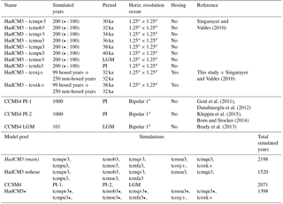

Table 2 GCM simulations.

3 Testing the PSR method

Here, we test the PSR method, first with synthetic data (Sect. 3.1), and then with the proxy records and model pools (Sect. 3.2) introduced in Sect. 2.2 and 2.3.

3.1 Synthetic PSR study

Before applying the PSR method on the proxy reconstructions, we perform a test with synthetic data. The synthetic data are 30 random disconnected climate states of the CCSM4 model output at the proxy locations. The number 30 is chosen to be small enough to perform a rapid test, while being larger than the low-pass filter applied on the model output. The results are comparable if a higher number is used instead. The climate states from the HadCM3 model pool serve as the model data pool. We follow the PSR method as described in Sect. 2.1 with the final surrogate reconstruction based on an average of 10 analogs. We perform such a reconstruction 1000 times in order to obtain robust statistics and find the distance between the PSR output and the original CCSM4 model output (regridded to HadCM3 grid) at each grid cell. This is presented as offsets in Fig. 3 at the 5, 50, and 95 percentiles.

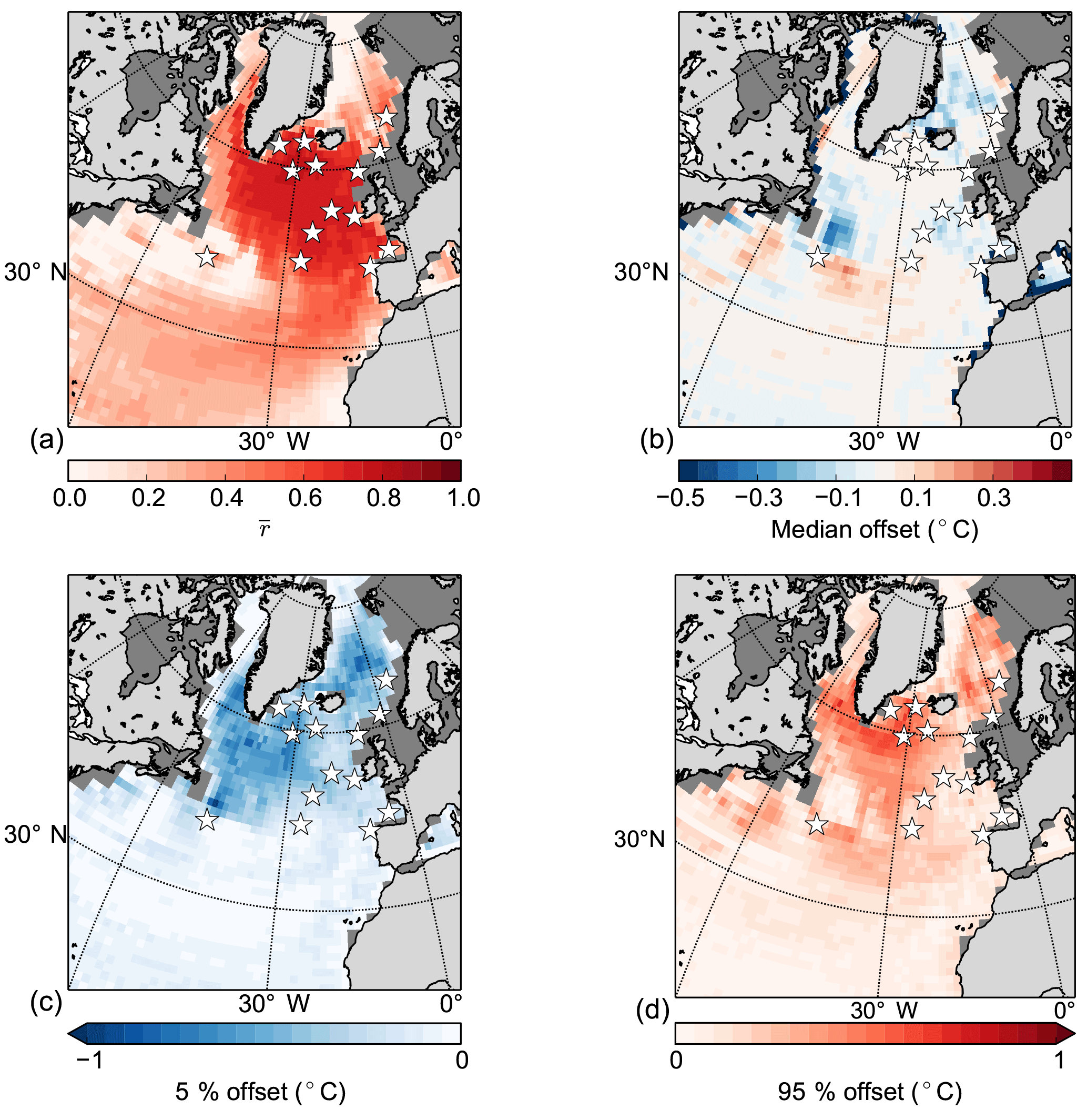
Figure 3 Synthetic PSR study. Colors show the (a) mean correlation coefficient between the synthetic data and the surrogate reconstruction, (b) the median, (c) the 5 and (d) 95 % offsets between the synthetic value and the reconstructed surrogate value. The synthetic observations are 30 random years from the CCSM4 model pool at the core locations; the model pool is HadCM3. This is repeated 1000 times. Grey shading represents the glacial coastline in the tcmoe3 simulation (Table 2, differs slightly between runs), while the white stars mark the core locations.

The good agreement between the PSR output and the original model output (Fig. 3) demonstrates that the spatially sparse synthetic data at the proxy locations can effectively recover the simulated ocean state in the surrounding ocean. The correlation between the surrogate reconstruction and the original model output exceeds 0.7 in the subpolar gyre region. In the rest of the North Atlantic, the correlation exceeds 0.5 except along the eastern coast of Greenland and along 35^∘ N. The reconstructed temperatures are generally within $\pm \mathrm{0.3}{}^{\circ }$C of the model output (Fig. 3b), but some of the reconstructed values are up to 1 ^∘C from the real value (Fig. 3c, d). This reflects the fact that the proxy locations do not provide enough information for the PSR method to fully recover the model output in these areas, and that some of the extremes in the synthetic data are poorly represented by the model pool. In general, these results act as a guide as we proceed to the proxy data.

3.2 Proxy data testing

3.2.1 Number of analogs

Several climate states from the model pools might match the proxy reconstructions well at the core locations, but differences away from the core sites might be large as different climate states can produce similar RMSE at the core locations (Fig. 4). Therefore, to ensure a consistent surrogate reconstruction, the composites are an average of a number of analogs with the smallest RMSE. As the number of analogs (N) increases, each additional member has less and less effect on the final 2-D pattern. As noted by Gómez-Navarro et al. (2017), the correlation between the proxy and the surrogate time series increases with N, while the standard deviation of the surrogate time series decreases with it. In our case, choosing N much larger than 10 results only in a small increase in correlation but in a large decrease in the standard deviation of the surrogate time series (Fig. 5a, correlation and standard deviation presented as a mean of the 14 core locations). On the other hand, choosing N less than 10 decreases the correlation of the time series. In addition, the lowest RMSE is obtained around N=10, the number of analogs which we use for the remainder of this study.

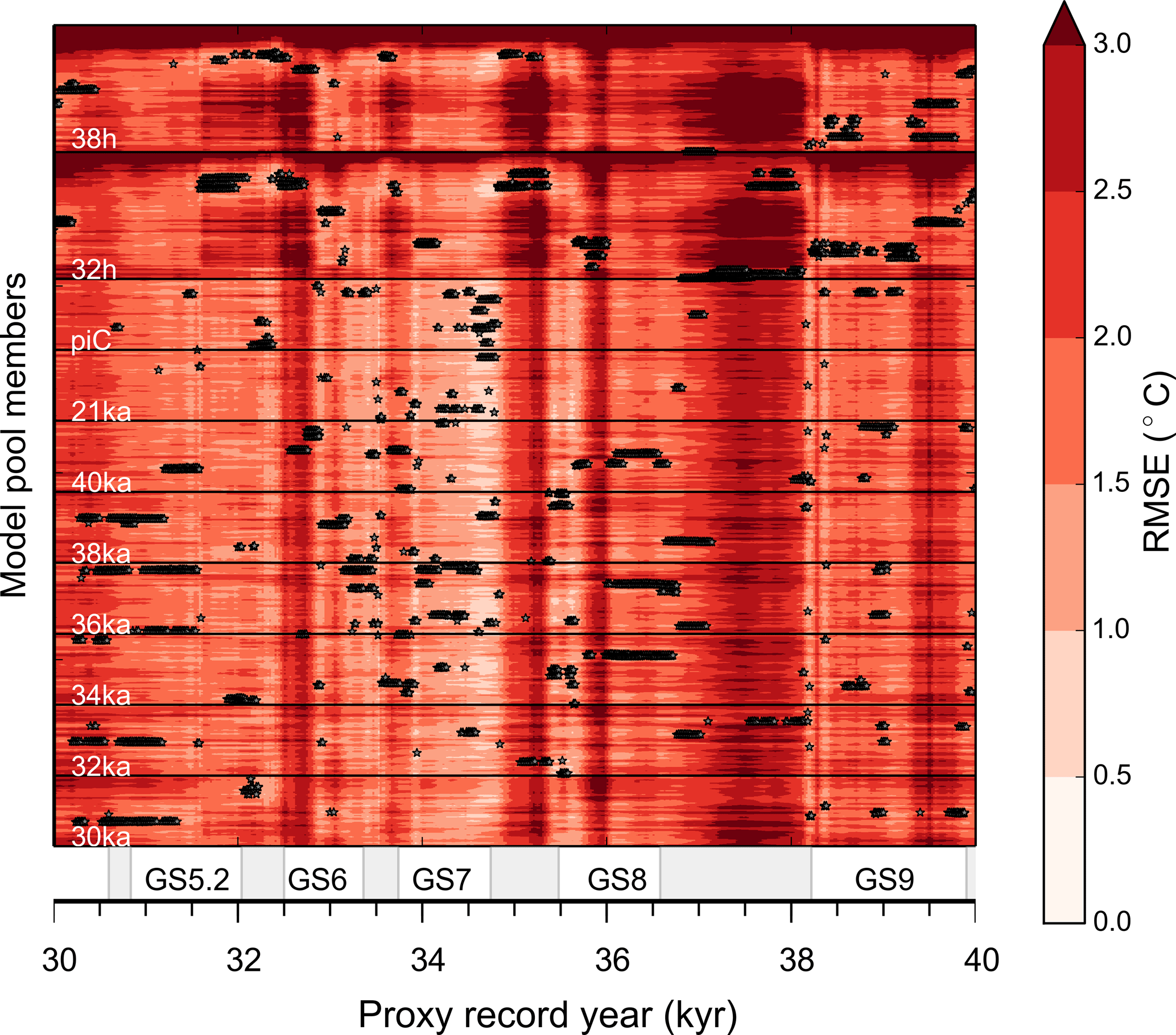
Figure 4 Colors show the RMSE between the main model pool and the SST-proxy data for each climate state (2198 in total, y axis) and proxy time step (501 in total, x axis). Black dots indicate the 10 model years (analogs) that constitute the composite for a given year in the surrogate reconstruction (i.e., the years with smallest RMSE). Thus, there are 10 black dots per column. Model members and respective simulations are indicated in white writing, and black lines separate the different simulations. The proxy time steps are indicated on the x axis where shaded grey areas mark the GIs, while the GSs are named.

Figure 5 Taylor diagram showing the agreement between the proxy data and the surrogate time series produced using (a) different number of analogs (1–30) using the main HadCM3 model pool. Increasing size of circles corresponds to increasing number of analogs. N=10 is marked in blue. (b) Different model pools (legend). The dashed black line indicates the standard deviation of the proxy data. Full black lines indicate the centered rms difference (labels, in ^∘C). All values are means over the 14 core locations where correlation and standard deviation are calculated for the 30–40 kyr time period.

3.2.2 Model pool

The correlation between the surrogate reconstructions and the corresponding proxy data is largely independent of the model pool, while the amplitude (standard deviation) of the variability depends on it (Fig. 5b, correlation and standard deviation presented as a mean of the 14 core locations). The surrogate reconstruction based on the full HadCM3 model pool outperforms the others with regard to the standard deviation and RMSE (Fig. 5b), which is why it is the main model pool in this study. The mean correlation between the proxy record and the surrogate time series at the core locations does not change when excluding the two hosing simulations from the model pool. However, the mean standard deviation of the surrogate time series at the core locations decreases from 0.98 with the main HadCM3 model pool to 0.67 with HadCM3 nohose. If the CCSM4 pool is used instead, the variability of the surrogate time series decreases further. For all model pools, the JAS average of the model data gives better results than annual means.

3.2.3 Model–proxy distance

Ideally, if the full model pool captures the variability of the proxy record, the best analogs are scattered among all possible climate states represented in the model pool and have equally low RMSE (Eq. 1) throughout the surrogate reconstruction. This is not the case throughout the record (Fig. 4), as generally colder periods are better captured by the model pool than warmer periods. The worst fit between the model and proxy data with respect to the RMSE is found during the time interval 36.9–38.3 kyr (same for all models; not shown). During this interval, the RMSE is large and the best analogs are constructed from very few different climate states which mainly belong to the hosing simulations. One could argue that this is an artifact that depends on the baseline from which we calculate the anomalies for both proxy and model data. Indeed, the mean of the proxy data is closest to stadial temperatures, and the amplitudes of the warm interstadials are larger than those of cold stadials in the proxy data. Therefore, a large RMSE during interstadials does not necessarily indicate that the model state is furthest from the interstadials, but rather that the model pool does not capture the full variability of the proxy record.

Nevertheless, because choosing a baseline from which we compute the anomalies is not trivial, we test three plausible alternatives.

For the original approach, we simply compute anomalies from the temporal mean:

$$\begin{array}{}\text{(5)}& \begin{array}{rl}{\displaystyle }& {\displaystyle }{T}_i^{{\mathrm{p}}^{\prime }}=T_i^{\mathrm{p}}-\stackrel{\mathrm{‾}}{T_i^{\mathrm{p}}},\\ {\displaystyle }& {\displaystyle }{T}_i^{{\mathrm{m}}^{\prime }}=T_i^{\mathrm{m}}-\stackrel{\mathrm{‾}}{T_i^m},\end{array}\end{array}$$

where the overline ($\stackrel{\mathrm{‾}}{\cdot }$) represents the mean, and the prime (^′) represents the anomaly (excluded in the other sections of the text for simplicity). Note that for the model pool the anomalies are with respect to each individual model simulation, not the full model pool.

One could argue that a reasonable way to calculate the proxy and model anomalies would be to compare them to PI (Holocene) conditions in order to avoid the bias toward stadial times. We have temperature reconstructions of PI conditions for nine of the cores for which we use the mean of the past 10 kyr as the baseline. We omit the proxy records for which we do not have this information. For the model pools, we use the mean of the PI control simulations. The anomalies become

$$\begin{array}{}\text{(6)}& {\displaystyle }& {\displaystyle }{T}_i^{{\mathrm{p}}^{\prime }}=T_i^{\mathrm{p}}-\stackrel{\mathrm{‾}}{T_i^{\mathrm{p}}}(\mathrm{0}-\mathrm{10}\mathrm{kyr}),\text{(7)}& {\displaystyle }& {\displaystyle }{T}_i^{{\mathrm{m}}^{\prime }}=T_i^{\mathrm{m}}-\stackrel{\mathrm{‾}}{T_i^{\mathrm{m}}}\left(\mathrm{PI}\right).\end{array}$$

Using the PSR method with these anomalies we find that the RMSE between the proxy data and the model simulations increases, and the mean correlation between the surrogate and proxy reconstructions at the core locations drops by 35 % (compared to the original definition but with only nine cores), and very few different model years are chosen for the analogs.

Finally, one could argue that a reasonable choice would be to use the stadial conditions as the baseline. Here, we compute the anomalies as

$$\begin{array}{}\text{(8)}& \begin{array}{rl}{\displaystyle }& {\displaystyle }{T}_i^{{\mathrm{p}}^{\prime }}=T_i^{\mathrm{p}}-\stackrel{\mathrm{‾}}{T_i^{\mathrm{p}}}(\mathrm{38.2}-\mathrm{39.9}\mathrm{kyr}),\\ {\displaystyle }& {\displaystyle }{T}_i^{{\mathrm{m}}^{\prime }}=T_i^{\mathrm{m}}-\stackrel{\mathrm{‾}}{T_i^{\mathrm{m}}}(\mathrm{MIS}\mathrm{3}\mathrm{nohose}\mathrm{sim}.).\end{array}\end{array}$$

As a result, the RMSE increases, and the mean correlation and standard deviation of the resulting surrogate reconstruction and proxy data at the core locations decrease. Neither the hosing simulations nor the PI or LGM simulations are chosen for the analogs. This is also true if Eq. (6) is normalized by the standard deviation of the stadial time period in addition. The definition of the anomaly is clearly important for the PSR method, but since the original definition (the temperature anomaly calculated with respect to the mean of the 30–40 kyr time period and the full simulations, for proxy and model data, respectively) performs the best, the following discussion will focus on it.

4 The proxy surrogate reconstruction

We now look at the results of the PSR both as time series at the core locations and as composite maps. Our interpretation of the results is found in Sect. 5.

4.1 Reconstruction at proxy locations

The performance of the surrogate time series at the different proxy locations differs between sites (Fig. 6, $r=\mathrm{0.4}-\mathrm{0.93}$; $A=\mathrm{0.31}-\mathrm{1.95}$, where A is the ratio between the standard deviation of the surrogate and proxy data time series), but for all but two cores the correlation between the surrogate time series and the proxy records exceeds 0.65. Surrogate time series taking into account possible uncertainties in the age models produce a confidence interval that generally follows the proxy time series. This is especially true for the long-lasting GS9 and GI8 where most of the surrogate time series produced with the original age models agree with the age model uncertainties at the core locations. We therefore focus on GS9 and GI8 when studying the spatial patterns using composite maps of the surrogate time series over these periods.

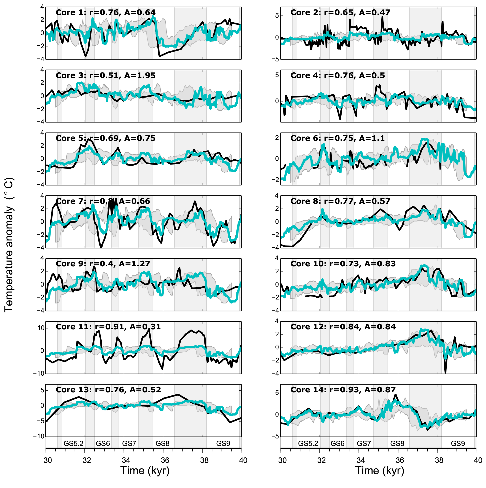
Figure 6 Surrogate time series (blue) and proxy time series (black) for all 14 core locations. All time series are plotted as anomalies from the mean value of the respective time series. The filtered, JAS-averaged SSTs from HadCM3 are used. Core numbers correspond to those shown in Fig. 1, and r is the correlation coefficient of the time series at each location. A is the ratio between the standard deviation of the two shown time series, $A=\mathit{\sigma }\left(c_i\right)/\mathit{\sigma }(T_i^{\mathrm{p}}$), where c_i and $T_i^{\mathrm{p}}$ are the surrogate and proxy reconstructions at location i, respectively. The grey shading around the surrogate time series is the 90 % confidence interval produced by shifting each proxy record individually by ±500 years (Sect. 2.2 for details). The vertical bars represent interstadial conditions in Greenland as defined by Rasmussen et al. (2014), and the GSs are named in the lowermost panels.

The surrogate reconstruction proves to be relatively independent of a single proxy time series. By excluding one core at a time before performing the PSR method, we can estimate the importance of each core in the full reconstruction. The mean correlation between the proxy data and the surrogate time series hardly changes and slightly improves in some cases ($\stackrel{\mathrm{‾}}{r}=\mathrm{0.72}-\mathrm{0.80}$) as there are fewer constraints on the surrogate reconstruction. By doing this, we can also assess the agreement between the proxy data and the surrogate time series at the location where the core was excluded (i.e., bootstrapping). Once again, the performance differs between sites, but the agreement between the two records is on average r=0.35.

4.2 Reconstructed spatial patterns

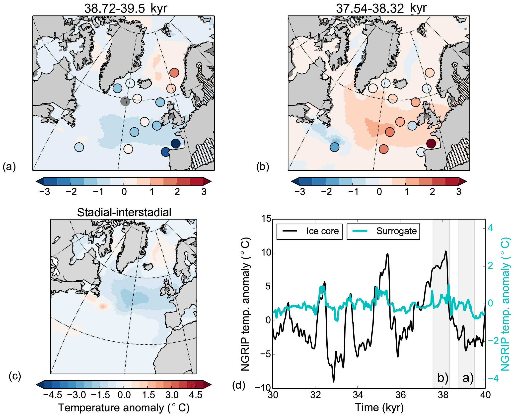
The surrogate reconstruction based on the full HadCM3 model pool shows lower SSTs during GS9 than during GI8 throughout the subpolar North Atlantic (Fig. 7). Notable exceptions are the subtropical–subpolar gyre boundary off the coast of North America which shows warmer conditions during GS9 than during GI8, and the northern Nordic Seas which show little to no temperature change. We note that the synthetic test in Sect. 3.1 showed that the variability in the subtropical–subpolar gyre boundary off the coast of North America was poorly represented by the variability at the core locations, and caution should be taken in interpreting the results at this location. During GI8, the subpolar gyre is warmer than the mean of the surrogate time series with especially strong warming near the Greenland–Scotland Ridge and the coast of western Europe. The results are robust for differences in age models and do not depend on single cores (see details in Fig. 7).

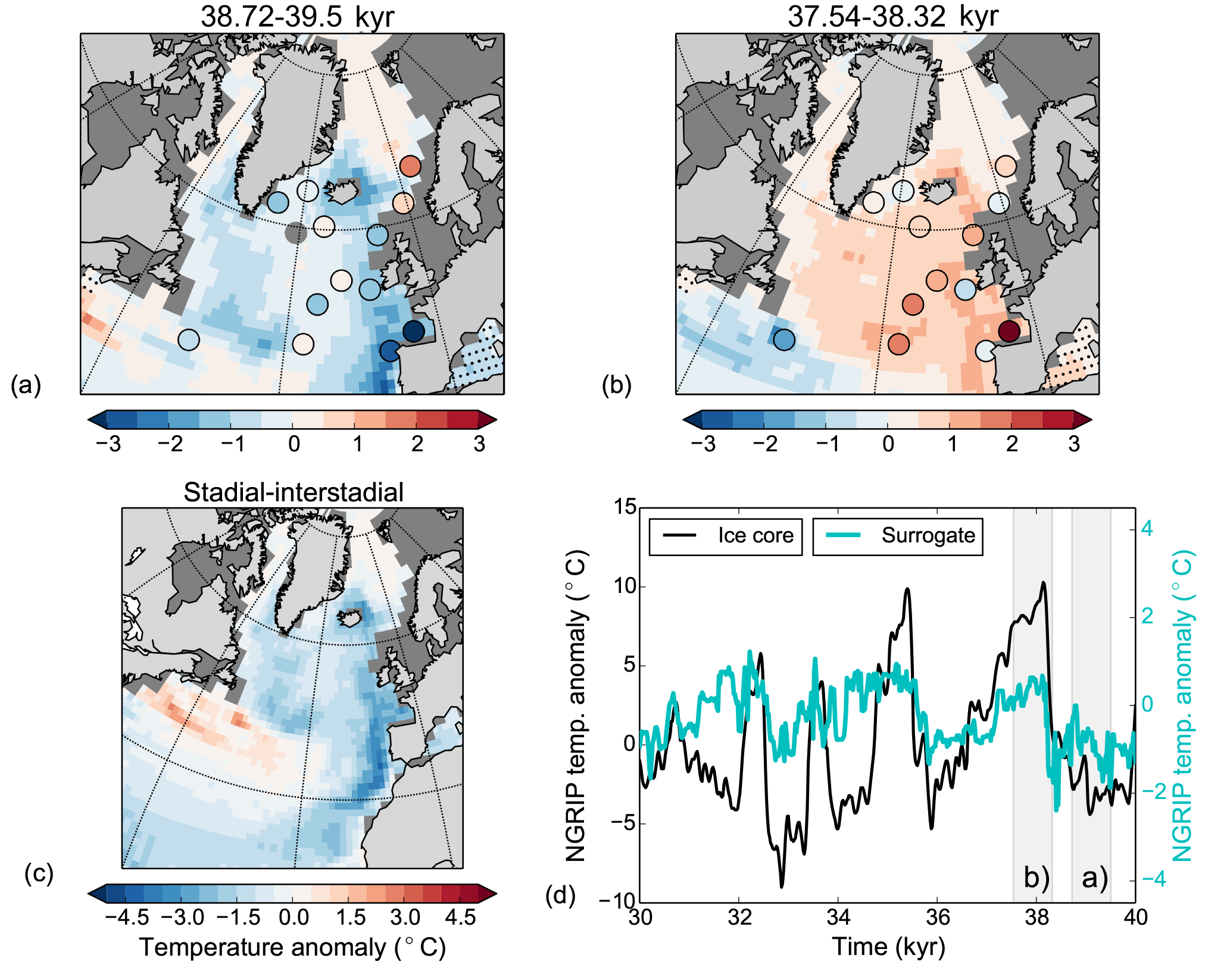
Figure 7 Temporal means of the spatial patterns for (a) end of GS9, (b) beginning of GI8, and (c) the GS9–GI8 difference. Background color shows the temperature anomalies from the surrogate reconstruction, while colors in circles indicate temperature anomalies from the proxy data (missing values for core 5 in the time period of panel (a). Black (yellow) dots mark points where the surrogate reconstruction using the original age models are not within the 90 % confidence level using age offsets of 500 years (dropping each core, all values within). Panel (d) shows reconstructed NGRIP temperatures from the ice core (black line, right y axis; Kindler et al., 2014) and the values from the surrogate time series (blue; note different y axis). The surrogate reconstruction is made using the same analog years which were picked for the SST reconstruction. The grey vertical shadings show the time periods used in the other panels.

The spatial SST patterns are largely consistent with the surrogate reconstructions produced using the other model pools. Both the CCSM4 pool and the HadCM3 nohose model pool produce comparable surrogate time series, albeit lacking the amplitude present in the main HadCM3 model pool. The temperature patterns are similar (Figs. 8, 9), although the Nordic Seas are warmer during GS9 than GI8, which is not clearly seen in the case where the HadCM3 model pool is used. We note that the general SST pattern holds when PI control simulations with NorESM and IPSL are used as the model pools (not shown). The similarity in reconstructed ocean patterns suggests that the ocean variability is based on physical mechanisms present in a wide range of simulations.

Figure 8 Same as Fig. 7 but for HadCM3 nohose.

Figure 9 Same as Fig. 7 but for CCSM4 data.

4.3 Extending the information to other climate variables

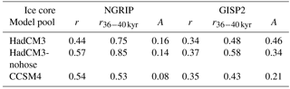
Given the reasonable agreement with the reconstructed SSTs and the original proxy records, we expand our analysis to other climate variables. We note that none of these variables are constrained by the PSR method, other than by being linked to the changing SSTs over the North Atlantic and the Nordic Seas. The ice-core temperature record from NGRIP (Kindler et al., 2014) and the reconstructed atmospheric temperature from the closest grid location to NGRIP in the surrogate time series are highly correlated (Fig. 7d, Table 3). Despite the high correlation, the amplitude of the temperature variability is much lower in the PSR record than in the ice-core record. However, since we are not able to capture the full amplitude of the temperature variability in the ocean, we do not expect to capture the full temperature variability in Greenland either. We note that the synthetic test in Sect. 3.1 gives a mean correlation of 0.74 between the PSR output and the original model output at the location of NGRIP. Also, the HadCM3 nohose and CCSM4 pools produce reasonable agreement with the ice-core record at NGRIP, although with a further decrease in the amplitude of the temperature variability, especially for the CCSM4 model pool (Figs. 8d, 9d, Table 3). The results of NGRIP are comparable if the surrogate reconstructions are compared to temperature reconstructions from the GISP2 ice core instead (Table 3; Cuffey and Clow, 1997; Alley, 2004).

Table 3 The agreement between the PSR and the ice-core record. A is the ratio between the standard deviation of the two time series.

The agreement between the reconstructed temperatures from ice cores in Greenland and the surrogate reconstruction shows that the PSR method has skill at reconstructing the climate in areas away from the core locations and in variables that are not directly linked to the SST proxies. Therefore, we now look at more variables and outside the core locations for GS9/GI8. Even though we do not aim to fully understand the dynamics of the variability, other variables might elucidate the mechanisms behind the oceanic variability we see.

We start by examining the ocean circulation with the AMOC variability of the surrogate reconstruction based on the HadCM3 model pool (Fig. 10), in which AMOC mostly varies with the strong freshwater forcing. The surrogate reconstruction consists of years from different states of the hosing runs: GS9 is best represented by the hosed conditions with weak AMOC, whereas GI8 is best represented by years just before or after the hosing. The beginning of GI8 tends to be best represented by the end of the hosing simulation as the AMOC resumes, while the end of the GI8 tends to be best represented by the beginning of the hosing simulations when the AMOC weakens (Fig. 4).

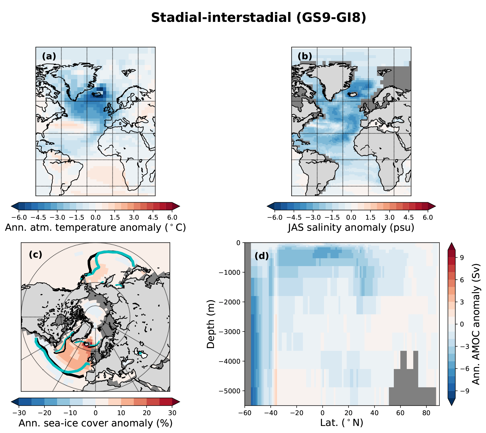
Figure 10 Composite of stadial–interstadial conditions (38.72–39.5 kyr vs. 37.54–38.32 kyr) for the surrogate time series constructed using the analogs picked with SSTs from the HadCM3 pool for panels (a–c) and HadCM3⋆ for panel (d). Colors show (a) annual atmospheric temperature anomalies, (b) JAS ocean salinity anomalies, (c) annual sea-ice cover concentration anomalies, and (d) annual AMOC anomalies. The black and blue contour lines in panel (c) are the 0.15 sea-ice concentration lines for stadial and interstadial, respectively, thick for March and thin for September.

The overturning stream function output was not available for all of the HadCM3 simulations, but we were able to continue the simulations lacking the output for another 100 years to recover the stream function output (note that these are simulations with constant forcing and boundary conditions, and we do not expect the AMOC properties to change from the original data). These simulations form a new model pool, HadCM3⋆ (Table 2), which enables a full AMOC reconstruction. We note that the PSRs based on HadCM3⋆ and HadCM3 are comparable (Fig. 5, similar RMSE and surrogate time series at core locations; not shown). The AMOC reconstruction shows a stronger overturning circulation during GI8 than during GS9; the whole upper cell of the stream function is weaker during GS9, apart from a negative cell in the Southern Ocean which behaves the opposite way (Fig. 10d). There is hardly any change in the overturning in the Nordic Seas. The same analysis with the HadCM3 nohose and CCSM4 model pools shows a generally stronger AMOC during GI8 than during GS9 (Figs. 11d, 12d). Interestingly, the HadCM3 nohose model pool shows a stronger overturning circulation over the Greenland–Scotland Ridge during GI8 than GS9 but a weaker Southern Ocean cell during GS9 than GI8. However, the HadCM3 nohose and CCSM4 model pools lead to AMOC changes that are generally very small. Due to the uncertainties in age models of the oceanic proxies, it is difficult to conclude whether the AMOC signal leads or lags the transitions between the GSs and GIs.

Figure 11 Same as Fig. 10 for the HadCM3 nohose model pool. Note the different limits on the colors compared to Fig. 10.

Figure 12 Same as Fig. 10 with the CCSM4 model pool. For clarity, only the contours of the March sea-ice extent are shown. Note the different limits on the colors compared to Fig. 10.

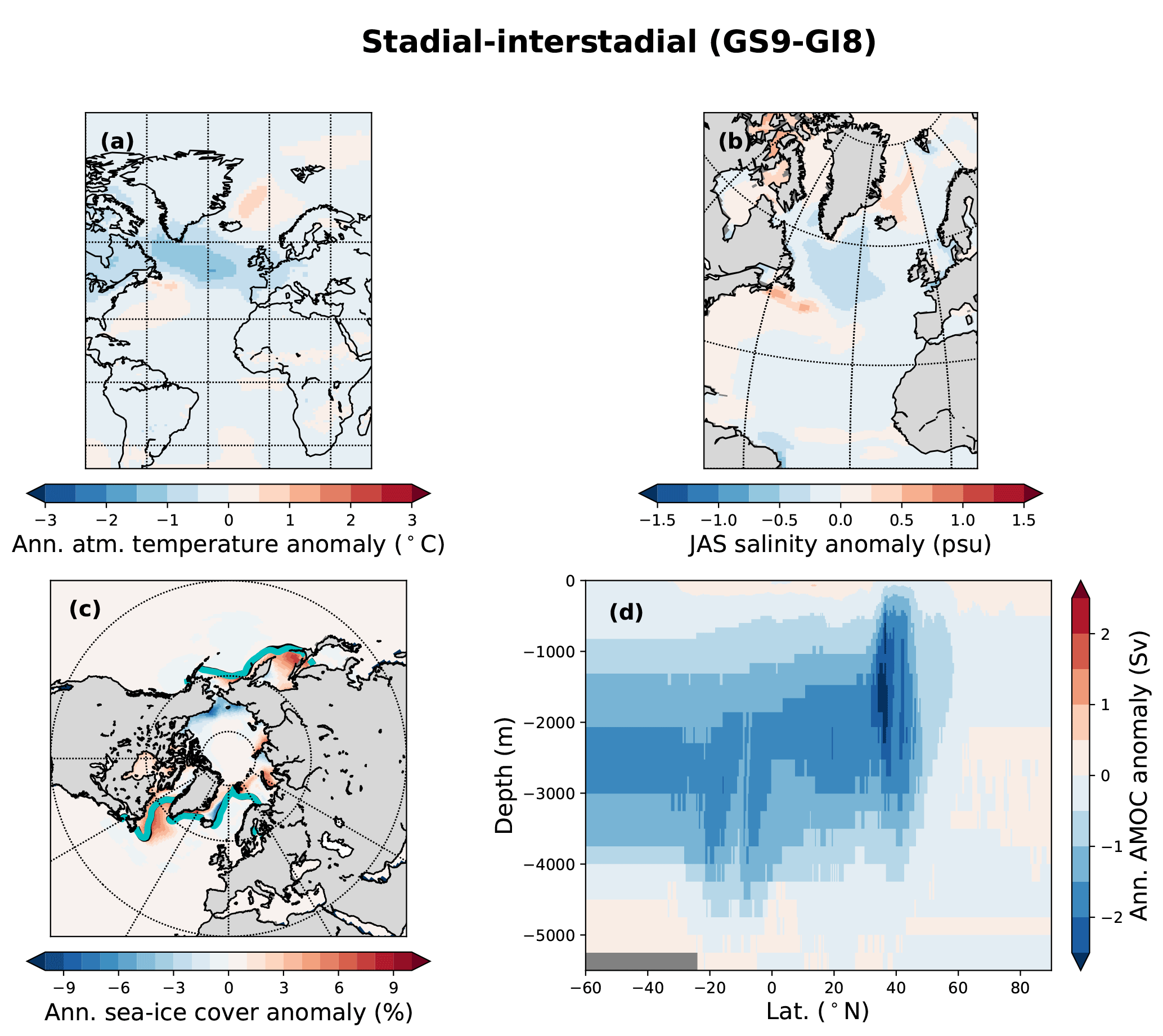
Sea-ice changes are largest for the main HadCM3 pool which includes hosing. There is a ∼ 20 % decrease in the annual sea-ice concentration in the subpolar gyre region between GS9 and GI8. The sea-ice edge retreats northwest during GI8, with largest change in the winter sea-ice edge (Fig. 10c). Close to the Greenland–Scotland Ridge, the annual mean sea-ice concentration changes are even larger (> 30 %) as parts of the area are perennially ice covered during GS9 but ice-free almost the whole year during GI8. For the model pools without the hosing simulations, the changes in the sea-ice cover are smaller (Figs. 11c, 12c). The HadCM3 nohose model pool produces a PSR with a east–west retreat in the sea-ice edge from GS9 to GI8 in the subpolar gyre region. For the CCSM4 model, the sea-ice changes are mostly visible as a shift in the summer sea-ice edge.

Consistent with the sea-ice changes and the freshwater forcing, the surrogate reconstruction shows a much fresher surface in the North Atlantic and the Nordic Seas during GS9 than GI8 (Fig. 10b). Indeed, the surrogate time series consist of model years taken from the beginning and end of the hosing simulations during GS9 and GI8, respectively (Fig. 4). Interestingly, the simulations without additional freshwater forcing also produce a fresher subpolar gyre during GS9 (Figs. 11b, 12b), although the freshening is much weaker and does not extend to the Nordic Seas as in the freshwater forced simulations.

Changes in the atmospheric temperature are similar to the changes in the SSTs. The HadCM3 model pool results in a colder atmosphere during GS9 than GI8 over much of the North Atlantic, with the cold conditions extending to Greenland, western Europe, and northern Africa (Fig. 10a). However, in the subtropical–subpolar gyre boundary and in the southern Atlantic, the atmosphere is warmer during GS9 than GI8, consistent with the AMOC changes. The strongest atmospheric anomalies are found near the Greenland–Scotland Ridge where the sea-ice changes are the largest. When the HadCM3 nohose and CCSM4 model pools are used, the atmospheric temperature signals are weaker, mostly confined to the North Atlantic Ocean and do not extend over land, except to parts of western Europe and eastern North America (Figs. 11a, 12a). For the HadCM3 nohose pool, a weak signature is also seen over parts of Greenland. For both model pools, the subpolar gyre region is colder during GS9 than GI8, but for the Nordic Seas and the subtropical–subpolar gyre boundary where the atmosphere is warmer during GS9 than GI8 (consistent with the SST changes).

5 Discussions

The PSR method is tested for the first time with proxy data from MIS3. We produce a new time series which is consistent with the information from the proxy data, although it is dependent on the relative dating between records. We have addressed the uncertainties in the age models for the different proxy records; however, each individual test could be further evaluated. We also note that the method gives quantitatively similar results when individual proxy records are excluded, suggesting that one poor age model would not throw off the results. We note that the age uncertainties of cores 3, 4, and 14 are considered larger than the ±500-year age uncertainty tested. However, the results are not very sensitive to these cores, as dropping all three of them produces a PSR with similar correlation coefficient and a higher standard deviation. Further testing could include the addition of noise to the records to see how robust the PSR is to errors in the proxy data. The method is also sensitive to how the anomalies used to compare proxy data and model output are defined, and care should be taken in finding the right analogs. One obvious limitation is the lack of long LGM and glacial simulations with different forcings. However, such simulations can easily be included in the model pool should they come available. In general, expanding the model pool is straightforward and would be a natural next step when new simulations become available, for example, through the Climate Model Intercomparison Project phase 6 (CMIP6; Otto-Bleisner et al., 2017; Kageyama et al., 2018).

We have shown that the PSR leads to a pattern of SST change from GS9 to GI8 which is largely independent of the underlying model pool. However, the results suggest that freshwater forced simulations are needed to capture the magnitude of the SST variability, although even these results are not able to capture the full amplitude of the proxy data. We suggest that these results have two interesting implications.

First, the pattern of SST variability can be reproduced across a wide range of model simulations including some with constant boundary conditions and external forcing. This suggests that SST patterns during DO events are not unlike those of modern internal variability. In the case of the HadCM3 model pool, the SST pattern is excited by freshwater forcing. However, we suggest that in the case of HadCM3 nohose and CCSM4 model pools a somewhat similar pattern results from an ocean response to a shift in the North Atlantic Oscillation (NAO), a prominent mode of atmospheric variability. Indeed, earlier studies have shown almost identical SST (Delworth and Zeng, 2016; Delworth et al., 2017) and sea-ice (Ukita et al., 2007) patterns as a response to changing NAO. However, despite the similar SST response pattern, the amplitude of the response associated with the NAO is not large enough to explain the SST variability seen in DO events. Therefore, we expect that other factors amplify the SST response pattern during DO events.

Second, the PSRs from the HadCM3 model pools are the only reconstruction where the GS9 to GI8 temperature difference is visible far beyond the North Atlantic Ocean. Previous literature (Broecker, 2000; Gildor and Tziperman, 2003; Masson-Delmotte et al., 2005; Li et al., 2005, 2010; Dokken et al., 2013; Hoff et al., 2016) suggests that changes in the sea-ice cover amplify the temperature response in Greenland over the DO transition. We suggest that the lack of a sea-ice change in the CCSM4 model-pool-based PSR is the primary reason for the weak temperature signal over Greenland in the surrogate reconstruction, and that the larger sea-ice changes in HadCM3 compared with HadCM3 nohose partly explain the better agreement with the proxy records for the former model pool. Similarly, the weaker-than-observed temperature variability in the HadCM3-based PSRs in Greenland is probably partly dependent on the amplitude and location of the changes in the sea-ice cover. Sea-ice reductions in the Nordic Seas have been shown to produce a larger temperature response in Greenland than sea-ice reductions in the subpolar gyre (Li et al., 2010), which is where we see the largest sea-ice changes. We also note that for the HadCM3 model pool, the largest changes in the sea-ice cover take place in winter, consistent with studies suggesting that winter sea-ice change is needed to capture the Greenland temperature variability (Li et al., 2005; Denton et al., 2005). However, for CCSM4, the change in the summer sea ice tends to be larger than the change in the winter sea ice.

While our results suggest that changes in the freshwater input to the North Atlantic could explain large parts of the glacial temperature variability in the North Atlantic and in Greenland, this does not necessarily imply that freshwater input is the only possible forcing of the glacial variability. Since the internal variability reproduces the patterns of glacial SST variability, although with a reduced amplitude compared to proxy data, it could be that any forcing that can excite such internal modes of variability could possibly contribute to the DO type of temperature change if the boundary conditions (e.g., sea ice) are right. The results suggest that even in the absence of freshwater forcing, GS9 is linked to anomalously fresh conditions in the cold subpolar gyre (Figs. 11b, 12b). Such fresh conditions provide a positive feedback that slows down the circulation and further cools the gyre, a feedback mechanism found to be important in both decadal and millennial climate variability (Born et al., 2010; Born and Levermann, 2010; Born et al., 2013; Moffa-Sánchez et al., 2014; Born et al., 2015). Therefore, even if the freshwater is not a primary forcing needed for glacial variability, internal freshwater feedbacks like the subpolar gyre response can still be an important amplifier of the glacial variability. Extending the model pool to simulations forced with other possible mechanisms could be used to further explore the importance of the freshwater forcing.

6 Conclusions

We have applied, for the first time, the proxy surrogate reconstruction method to oceanic proxy data from MIS3. The results are robust to different sensitivity tests and relatively independent of the underlying model data and proxy locations.

Our results imply that the patterns of oceanic variability in the glacial climate can be well represented by patterns of short-term variability intrinsic to the climate system. We find consistent patterns of variability in sea-surface temperature, sea-surface salinity, and atmospheric temperature in two different climate models and in different background climates. However, to fully capture the amplitude of the North Atlantic sea-surface temperature variability, forced simulations, in our case by freshwater, are required.

Our results further suggest that the sea-ice cover could play an amplifying role during DO events. We see a clear reduction in sea-ice concentration between stadial and interstadial conditions when the glacial simulations are included in the proxy surrogate reconstruction, likely contributing to the temperature signal in Greenland. Indeed, the lack of a large sea-ice signal might be one of the reasons why the model results without freshwater forcing lack the amplitude of the DO variations, especially in Greenland.

The analysis shows that the surrogate reconstruction can be used to combine model simulations and proxy data without having to assume the same climatic changes at all locations. In the North Atlantic, where the data coverage during MIS3 severely limits the usefulness of other data assimilation and inversion techniques, the PSR method is an especially useful method. As the method allows for the full non-linearity of the climate system, as represented by the coupled model simulations, we are able to capture a large part of the glacial variability in the ocean during MIS3 and also in Greenland. The method is an efficient offline data assimilation technique which allows for the quantification of uncertainty, unlike expensive transient simulations, which makes it a good first step for understanding the spatial variability of the climate changes seen during MIS3. Until the time that full complexity models are capable of simulating the full transient evolution of the climate over long periods, such simplified approaches will be crucial to our understanding of the climate.

Finally, we are well aware of the limitations of the methodology and the validation so far back in time. Therefore, we see this study as an encouraging first attempt to apply the PSR method to oceanic variability during MIS3 and believe it should be further developed for an ideal implementation. A straightforward next step would be to expand the model pool with simulations from different models and with different boundary conditions.