Recent climate variations in Chile: constraints from borehole temperature profiles

We have compiled, collected, and analyzed 31 temperature–depth profiles from boreholes in the Atacama Desert in central and northern Chile. After screening these profiles, we found that only nine profiles at four different sites were suitable to invert for ground temperature history. For all the sites, no surface temperature variations could be resolved for the period 1500–1800. In the northern coastal region of Chile, there is no perceptible temperature variation at all from 1500 to present. In the northern central Chile region, between 26 and 28^∘ S, the data suggest a cooling from ≈ 1850 to ≈ 1980 followed by a 1.9 K warming starting ≈ 20–40 years BP. This result is consistent with the ground surface temperature histories for Peru and the semiarid regions of South America. The duration of the cooling trend is poorly resolved and it may coincide with a marked short cooling interval in the 1960s that is found in meteorological records. The total warming is greater than that inferred from proxy climate reconstructions for central Chile and southern South America, and by the PMIP3-CMIP5 surface temperature simulations for the north-central Chile grid points. The differences among different climate reconstructions, meteorological records, and models are likely due to differences in spatial and temporal resolution among the various data sets and the models.

1 Introduction

To assess and predict the long-term effects of the modern climate warming, it is crucial to simulate and understand Earth's complex climate and its variability. Most of the inferences on the future evolution of the climate system come from large-scale general circulation model (GCM) simulations. Experiments with GCMs allow for the study of future climate under different scenarios. Due to the limited resolution of GCMs, climatically relevant processes that operate at less than the GCM grid size scale are not parameterized in the same way by different models. These different parameterizations lead to a wide variability in results among simulations by different GCMs. Hence, there is a need to test models against paleoclimate reconstructions and to assess the robustness of their climate projections.

As the meteorological record only extends back as far as 150 years or less, climate reconstructions based on proxy data are required to evaluate the performance of GCMs and provide insight into the long-term trends of climate variables. In contrast to the Northern Hemisphere where a lot of paleoclimatic reconstructions are available (e.g., Mann et al., 1999; Moberg et al., 2005; Rutherford et al., 2005), fewer climate reconstructions have been performed for the Southern Hemisphere and those rely on a small number of data sets (Huang et al., 2000; Mann and Jones, 2003; Intergovernmental Panel on Climate Change, 2013). In absence of paleoclimatic data, the forcing of the Southern Hemisphere's climate system is poorly known. Several studies have been initiated to fill in this gap but they continue to underscore the need for more paleoclimate records from the Southern Hemisphere (e.g., Villalba et al., 2009; Neukom and Gergis, 2012; Suman et al., 2017; Suman and White, 2017).

South America is a key continent for understanding the climate system of the Southern Hemisphere as it is the largest landmass in the Southern Hemisphere, extending from 10^∘ N to 55^∘ S. Flanked by the Andes to the west, the continent separates the Atlantic and Pacific oceans, influencing oceanic and atmospheric circulations, and global climate. There are few paleoclimatic data in South America and those are restricted to the southern portion of the continent, which may bias our understanding of the region.

Studying the climate of northern Chile is key to understanding how extremely sensitive arid environments respond to climatic variations. Furthermore, the natural resources and ecosystem of northern Chile have been put under ever increasing stress by the accelerating economic development of the region (Messerli et al., 1997). It is, therefore, of paramount importance to understand the long-term climatic variations of the region. There have been some regional paleoclimatic studies in northern Chile with the majority of them addressing the mid-Holocene paradox. In order to study the climate of northern Chile and South America of the past 500 years, we have compiled and collected borehole temperature–depth profiles, interpreted these data and determined ground surface temperature (GST) variations, and compared our results with climate reconstructions from other proxies and with climate model simulations.

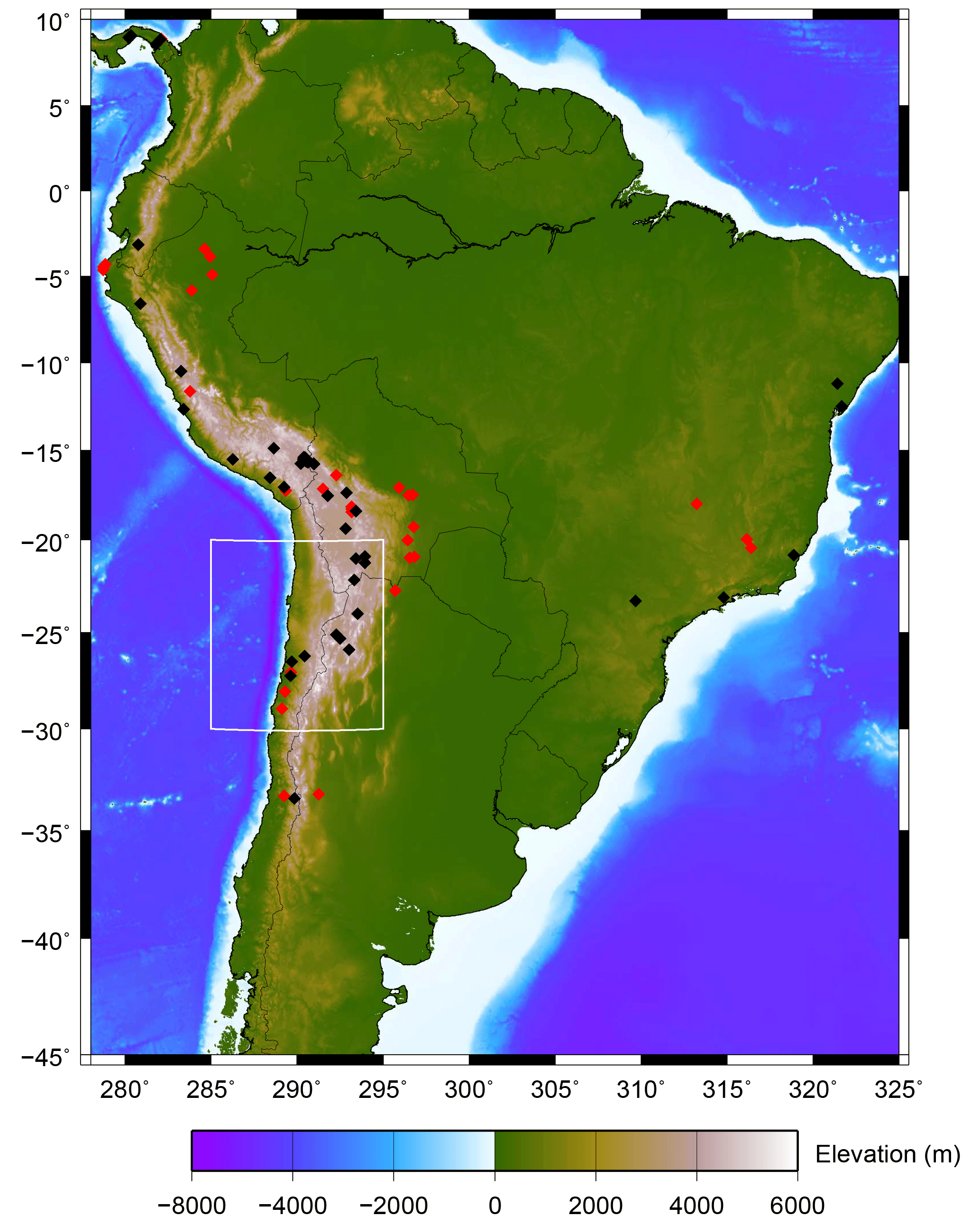
Figure 1 Map of South America including locations of borehole temperature measurements for heat flow studies from the updated International Heat Flow Commission (IHFC) (International Heat Flow Commission, 2011, http://www.datapages.com/gis-map-publishing-program/gis-open-files/global-framework/global-heat-flow-database, last access: 19 June 2017) database. Red diamonds represent boreholes deeper than 200 m, while black is boreholes shallower than 200 m. More than 100 bottom-hole temperature measurements, mainly in Brazil, are not included as they are not useful for climate studies. The rectangle indicates the study region of northern Chile.

The use of borehole temperature–depth profiles to determine past changes in GST and study past climate is relatively recent and was motivated by the concerns about rising global temperatures (Lachenbruch and Marshall, 1986; Lachenbruch, 1988). Over the years, many global, regional, and local reconstructions of GST have been undertaken (Huang et al., 2000; Harris and Chapman, 2001; Pollack and Smerdon, 2004; Jaume-Santero et al., 2016; Pickler et al., 2016). These studies have relied almost exclusively on temperature–depth profiles collected for heat flow measurements with two caveats: (1) not all the data are suitable for climate studies, and (2) heat flow data are very unevenly distributed with the vast majority being located in the Northern Hemisphere. A recent compilation of conventional land heat flow measurements shows that out of 17 232 heat flow values, 16 062 are found in the Northern Hemisphere and only 1170 in the Southern Hemisphere (Francis Lucazeau, personal communication; see also Jaupart and Mareschal, 2015). The compilation includes a total of 261 values for the entire South American continent where several large regions are void of measurements (Fig. 1). Beginning in the late 1960s, studies were conducted on the western margin of the continent to understand the heat flow of the arc–trench system (Uyeda and Watanabe, 1970; Watanabe et al., 1980; Uyeda and Watanabe, 1982). Unfortunately, most of the temperature profiles are too shallow and too coarsely sampled to be useful for climate studies. In addition, there are no digital archives of these data, but only figures in publication. More recently, Springer and Förster (1998) conducted a new heat flow study based on 74 temperature–depth profiles measured in Bolivia and northern Chile. We have selected some of these data to include in our analysis. Measurements were also made in Brazil (Vitorello et al., 1980) but some of the data are in publications of limited accessibility (Hamza et al., 1987). Despite the uneven sampling, Huang et al. (2000) inferred a cumulative temperature increase of 1.4 K over the past 500 years in South America from their global reconstruction of GST variations in the continents. Because this study relied on only 16 borehole temperature–depth profiles for South America, additional data are needed to confirm its conclusions. Hamza and Vieira (2011) selected and analyzed, in terms of GST variations, more than 30 temperature–depth profiles deeper than 200 m from eastern Brazil, the Amazon region, the Cordilleran region of Colombia, and the Cordilleran region of Peru. They inferred a warming of 2–3.5 ^∘C from the early 20th century to present and observed similar trends in tropical and subtropical zones. Meanwhile, a warming of 1.4–2.2 ^∘C from the late 19th century to present was inferred for the semiarid zones.

In an attempt to enlarge the South American borehole temperature data set, we have collected 31 borehole temperature–depth profiles measured in 1994, 2012, and 2015 in northern Chile, a region that was void of data, and reconstructed the GST history for the past 500 years. We compare these reconstructions with meteorological data for the region, past climate inferences based on proxy data, and model simulations for central Chile and southern South America to determine climate trends for northern Chile and assess their robustness.

2 Ground surface temperature reconstructions from borehole temperature profiles

To determine GST histories from temperature–depth profiles, we use a physical model of heat diffusion in the subsurface. We assume that Earth is a half space where physical properties vary solely with depth, heat is transported only by vertical conduction, and changes in the surface temperature boundary condition propagate into the subsurface and are recorded as temperature perturbations, T_t(z), of the steady-state (reference) temperature profile. The temperature, T(z), at depth z can then be written as (Jaupart and Mareschal, 2011)

$$\begin{array}{}\text{(1)}& T\left(z\right)=T_{\mathrm{o}}+q_{\mathrm{o}}R\left(z\right)-\underset{\mathrm{0}}{\overset{z}{\int }}{\displaystyle \frac{\mathrm{d}{z}^{\prime }}{\mathit{\lambda }\left(z^{\prime }\right)}}\underset{\mathrm{0}}{\overset{z^{\prime }}{\int }}H\left(z^{\prime \prime }\right)\mathrm{d}{z}^{\prime \prime }+T_{\mathrm{t}}\left(z\right),\end{array}$$

where T_o is the steady-state (reference) GST, q_o is the reference heat flux, λ(z) is the thermal conductivity, H(z) is the radioactive heat production, and T_t(z) is the temperature perturbation at depth z due to time variations in surface temperature. The effect of heat production is usually negligible for shallow depth. R(z) is the thermal resistance, which is defined as

$$\begin{array}{}\text{(2)}& R\left(z\right)=\underset{\mathrm{0}}{\overset{z}{\int }}{\displaystyle \frac{\mathrm{d}{z}^{\prime }}{\mathit{\lambda }\left(z^{\prime }\right)}}.\end{array}$$

The temperature perturbation, T_t(z), can be written as (Carslaw and Jaeger, 1959)

$$\begin{array}{}\text{(3)}& T_{\mathrm{t}}\left(z\right)=\underset{\mathrm{0}}{\overset{\mathrm{\infty }}{\int }}{\displaystyle \frac{z}{\mathrm{2}\sqrt{\mathit{\pi }\mathit{\kappa }{t}^{\mathrm{3}}}}}\exp \left({\displaystyle \frac{-z^{\mathrm{2}}}{\mathrm{4}\mathit{\kappa }t}}\right)T_{\mathrm{o}}\left(t\right)\mathrm{d}t,\end{array}$$

where κ is the thermal diffusivity, and T_o(t) is the surface temperature at time t before present. For a stepwise change ΔT in surface temperature at time t before present, the temperature perturbation, T_t(z), is given as (Carslaw and Jaeger, 1959)

$$\begin{array}{}\text{(4)}& T_{\mathrm{t}}\left(z\right)=\mathrm{\Delta }T\mathrm{erfc}\left({\displaystyle \frac{z}{\mathrm{2}\sqrt{\mathit{\kappa }t}}}\right),\end{array}$$

where erfc is the complementary error function. In order to parameterize the variations in surface temperature, T_o(t), we approximate them by their average values, ΔT_k, during K time intervals ($t_{k-\mathrm{1}},t_k$). The perturbation, T_t(z), is then obtained as follows:

$$\begin{array}{}\text{(5)}& T_{\mathrm{t}}\left(z\right)=\sum _{k=\mathrm{1}}^K\mathrm{\Delta }{T}_k\left(\mathrm{erfc}{\displaystyle \frac{z}{\mathrm{2}\sqrt{\mathit{\kappa }{t}_k}}}-\mathrm{erfc}{\displaystyle \frac{z}{\mathrm{2}\sqrt{\mathit{\kappa }{t}_{k-\mathrm{1}}}}}\right).\end{array}$$

The ΔT_k values represent the difference between the average GST during the time interval ($t_{k-\mathrm{1}},t_k$) and T_o.

2.1 Inversion

In order to reconstruct the GST history, Eqs. (3) (in which heat production is neglected) and (5) are combined to obtain one linear equation for each measured depth (z) with K+2 unknowns, T_o, q_o, and ΔT_k. The inversion involves solving the system of equations for the unknown parameters. This can be carried out either by (1) solving for the K+2 unknown parameters simultaneously or by (2) independently determining T_o and Γ_o, the reference GST and reference temperature gradient. We have made tests to compare the two techniques and found no significant differences among the results. For this study, we have used the second technique. T_o and Γ_o are calculated by linear regression of the lowermost 100 m of the temperature–depth profile. The lowermost 100 m of the temperature–depth profile is used since it is sufficiently deep to be unaffected by short period (<100 years) surface temperature perturbations and represent the geothermal steady state on a ≈100-year timescale. Furthermore, we made tests to check that the reference GST is stable and the reference heat flux does not vary with depth interval selected. An estimate of the maximum error at a 95 % confidence interval of T_o and Γ_o is also provided by the linear regression and gives the upper and lower bounds of the geothermal quasi-steady state, referred to as the extremal steady states. The temperature anomaly or perturbation T_t is then obtained by subtracting the linear fit from the data. If N temperature measurements were made, we obtain a system of N linear equations with K unknowns: the K values of ΔT_k. Regardless of the actual values of K and N, this system of equations is ill-conditioned and its solution is unstable. To stabilize the solution, various regularization techniques have been used (singular value decomposition, Backus–Gilbert inversion, Tikhonov regularization) and applied to GST history reconstructions (e.g., Mareschal and Beltrami, 1992; Vasseur et al., 1983; Wang et al., 1992). We use singular value decomposition (SVD) (Lanczos, 1961) because its application to GST inversion is straightforward. See Mareschal and Beltrami (1992) and Clauser and Mareschal (1995) for more details.

2.2 Simultaneous inversion

Simultaneous inversion is used at sites with multiple profiles. If the same temperature variations have affected the surface of the site, the profiles are expected to show consistent subsurface temperature anomalies. If the noise is random, inverting these profiles simultaneously for a common GST history results in increasing the signal-to-noise ratio and reinforcing consistent trends in the temperature anomalies. This technique has been widely used and is discussed further in Beltrami and Mareschal (1992), Clauser and Mareschal (1995), and Beltrami et al. (1997).

Figure 2 Map of northern Chile with locations of boreholes used in this study. The number of boreholes at each site is indicated in parentheses. Red circles indicate borehole temperature–depth profiles measured in 1994, black triangles are measured in 2012, and white diamonds are measured in 2015. Sites with borehole temperature–depth profiles deemed suitable for climate are Michilla, Totoral, Inca de Oro, and Vallenar.

Table 1 Location and technical information concerning the borehole temperature–depth profiles measured in 1994 by Springer (1997) and Springer and Förster (1998), in 2012 by Gurza Fausto (2014) and in 2015, where the column “suitable climate?” indicates if it passed the selection criteria outlined in Sect. 3.

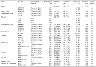
^a Value in parentheses indicates sampling interval and yields temperature measurements with a precision of 0.01 ^∘C.
^b Temperature measurements with a precision of 0.3 ^∘C.
^c Value in parentheses indicates continuous sampling and yields temperature measurements with an accuracy of 0.05 ^∘C.
^d Value in parentheses indicates sampling interval and yields measurements with a precision better than 0.005 K and an accuracy on the order of 0.02 K.
^e Temperature measurements with a precision of 0.3 ^∘C.

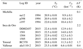
Table 2 Summary of inversion results where T_o is the long-term surface temperature, Γ_o is the quasi-steady-state temperature gradient, and ΔT is the difference between the maximal temperature and the temperature at 1500 years CE.

3 Data collection and selection

At 11 sites in northern Chile, 31 borehole temperature–depth profiles varying in depth from 118 to 557 m have been obtained (Fig. 2). One site includes one or several boreholes within a radius of 1 km or less. All the sites used in this study are located in the Atacama Desert, an arid region with little to no vegetation, and the holes had been drilled for mining exploration purposes. The temperature profiles were measured during three different campaigns in 1994, 2012, and 2015 (Springer, 1997; Springer and Förster, 1998; Gurza Fausto, 2014; Pickler et al., 2017). The data were obtained using different measurement techniques. Fiber-optic distributed temperature sensing (DTS), used for some holes in 1994 and 2015, is based on the measurement of a backscattered laser light pulse through a fiber-optic cable (Förster et al., 1997; Förster and Schrötter, 1997). It allows the continuous measurement of the entire profile once the cable has been completely lowered into the borehole. A detailed description of this methodology can be found in Förster et al. (1997), Förster and Schrötter (1997), Hausner et al. (2011), and Suárez et al. (2011). The remaining profiles were measured using the conventional method of lowering a calibrated thermistor into the borehole and measuring temperature with depth. In 2012, temperature was measured continuously by lowering the thermistor into the borehole at an average speed of ≈ 10–15 m min⁻¹. In 1994 and 2015, temperature was measured at 2 and 10 m intervals, respectively, with a precision of ±0.01 K. For the analysis, all profiles were resampled at 10 m intervals to ensure they were weighted evenly. Förster et al. (1997) and Wisian et al. (1997) ran tests to verify the consistency between the DTS and conventional methods. An offset among the temperature–depth profiles was detected and attributed to the calibration of the measurement tools. This effect is considered unimportant when examining temperature differences but must be accounted for to avoid an offset of the reference surface temperature. Information about all the profiles, including their locations, depths, and elevations, is provided in Tables 1, 2, and A1.

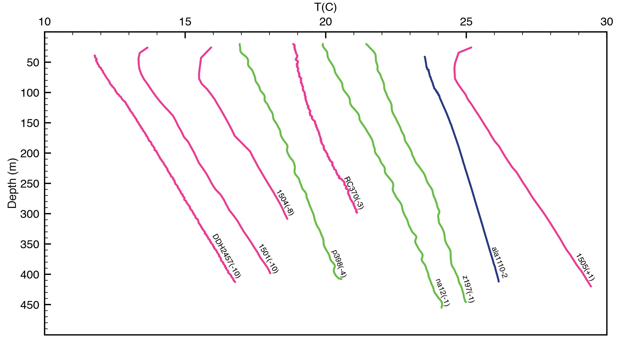
Figure 3 Retained temperature–depth profiles measured in 1994 (green), 2012 (blue), and 2015 (pink). Temperature scale is shifted as indicated in parentheses. The profiles from Michilla measured with DTS (in green) appear to be noisier than those obtained from conventional methods.

Figure 4 Temperature anomalies for the retained temperature–depth profiles, where IDO is Inca de Oro. The pink and blue lines represent the upper and lower bounds of the temperature anomaly. These are not visible at IDO-DDH2457 and Vallenar ala1110-2 because they are superimposed.

We used several selection criteria to determine whether the borehole temperature–depth profiles are suitable for climate studies, and ended up rejecting 20 profiles (Table A1 in Appendix). In the tectonic setting of the active central Andean orogeny, uplift and erosion occur that can alter the temperature gradient (Jeffreys, 1938; Benfield, 1949; Jaupart and Mareschal, 2011), but these effects take place on a much longer timescale than the 500-year period studied here and they can be considered negligible. In order to reconstruct 500 years, boreholes must be at least 300 m deep and to detect the recent changes they must include measurements in the topmost 100 m. Profiles less than 300 m deep and/or without measurements in the upper 100 m were rejected. Also, profiles were visually inspected to ensure that they show no discontinuities, signs of water flow, or other perturbations that would make them unsuitable for climate reconstructions. As topography distorts the temperature isotherms (Jeffreys, 1938), profiles on or near a slope steeper than 5 % over a distance comparable to borehole depth were rejected. This left only 11 profiles suitable for climate studies. However, two of the retained profiles are repeat measurements and do not provide independent information. The measurements of temperature at the Vallenar site (ala1110/ala1110-2) used the same technique (conventional method with continuous sampling) and yielded identical profiles. We arbitrarily retained profile (ala1110-2).

At the Inca de Oro site, where hole DDH2489A was logged using a conventional thermistor and DTS, we retained the conventional measurements (1501) because they have better temperature resolution (0.01 K) than the DTS (0.1 K).

Following this selection, we retained nine independent profiles suitable for inversion (Fig. 4). We truncated the profiles at 300 m to ensure that we were referring to the same time period, and we calculated the temperature anomalies (Fig. 4). These profiles are distributed among four sites: one (Michilla) in northern coastal Chile was measured in 1994, and a group of three (Inca de Oro, Totoral, Vallenar) in north-central Chile were measured in 2012 and 2015 (Fig. 2). Northern coastal Chile and north-central Chile are more than 500 km apart. The three Michilla boreholes are located in a relatively flat area near the Michilla open pit mine, ≈ 10 km from the coast. The dominant lithologies crossed by the holes are andesite and diorite (Springer, 1997; Springer and Förster, 1998). The other three sites (Inca de Oro, Totoral, Vallenar) are located between 26 and 28^∘ S. Four boreholes were logged in the center of a flat basin between two ranges ≈ 5 km away near the town of Inca de Oro, less than 100 km from the coast. The Totoral borehole is located in a relatively flat area, ≈ 75 km southwest of the city of Copiapó and ≈ 50 km from the coast. The borehole at Vallenar is located between two hills, ≈ 20 km southwest of the city of Vallenar and ≈ 40 km from the coast. All the holes that we logged in north-central Chile had been drilled through sediments and penetrated only a few meters in the crystalline basement. The only lithological log available (for borehole RC370, Totoral) shows that a dominant lithology of sandstone with no significant lithological changes. Cuttings picked near the Inca de Oro boreholes showed similar lithologies.

Previous heat flow measurements made in Chile in 1969 included several holes in the region of Vallenar (Uyeda et al., 1978; Uyeda and Watanabe, 1982). A digital archive of these measurements could not be found and the profiles are too shallow (< 200 m) to be very useful in climate studies. The Vallenar data show small temperature gradients (≈10 K km⁻¹) and very low heat flux (≈20 mW m⁻²), which are consistent with our measurements.

For measurements made in 1994, Springer and Förster (1998) found a mean thermal conductivity of 2.04 W mK⁻¹ for the three Michilla boreholes and noted no significant thermal conductivity variations. Because the holes had been drilled by percussion no continuous core was retrieved from the holes at the Inca de Oro and Totoral sites measured in 2012 and 2015 and we could not make conductivity measurements. The calculated temperature gradients showed no obvious signs of thermal conductivity variations. For the borehole RC370, no major change in conductivity with depth is consistent with the lithological log that shows no significant change in lithology.

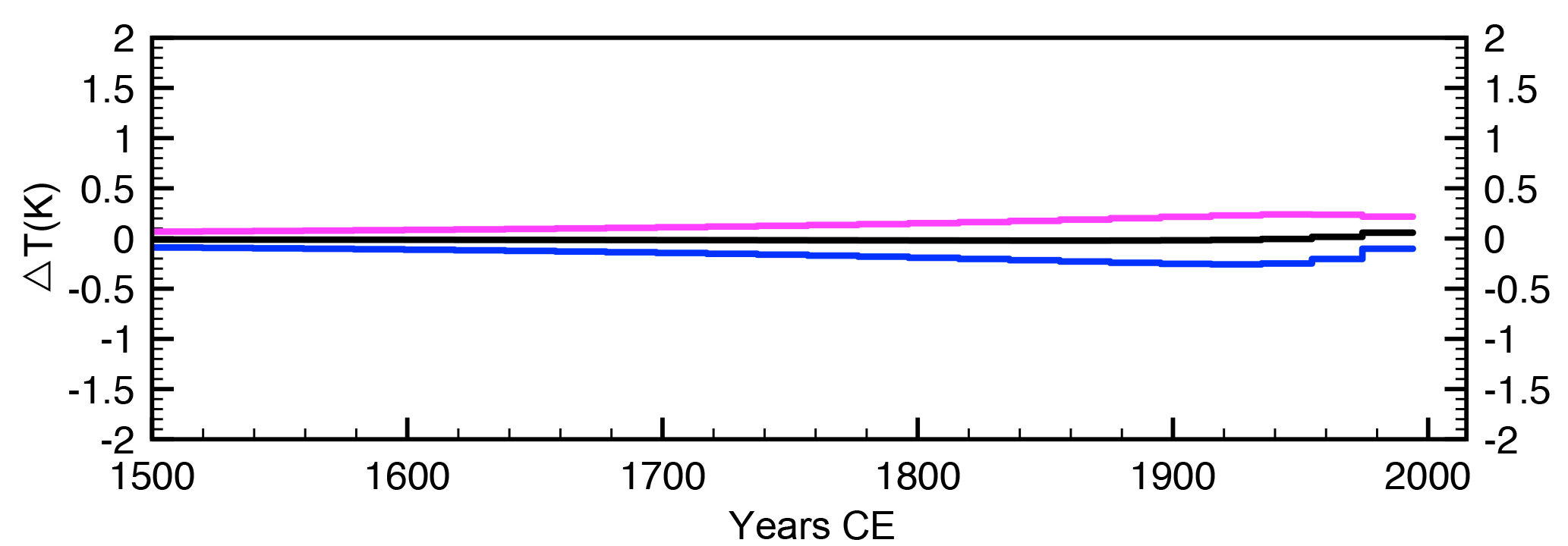
Figure 5 GST history for northern coastal Chile (Michilla) determined for its period of measurement (1994) from the simultaneous inversion of na12, p398, and z197, where three eigenvalues are retained. The pink and blue lines represent the inversion of the upper and lower bounds of the temperature anomaly or the extremal steady states.

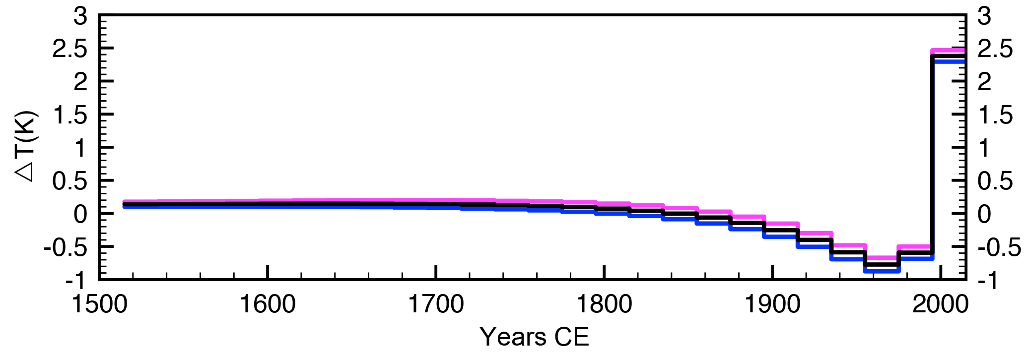
Figure 6 GST history for Inca de Oro determined from the simultaneous inversion of DDH2457, 1501, 1504, and 1505, with three eigenvalues retained. The pink and blue lines represent the inversion of the upper and lower bounds of the temperature anomaly or the extremal steady states.

Figure 7 GST history for Totoral (RC370), with three eigenvalues retained. The pink and blue lines represent the inversion of the upper and lower bounds of the temperature anomaly or the extremal steady states.

Figure 8 GST history for Vallenar (ala1110-2), with three eigenvalues retained. The inversion of the upper and lower bounds of the temperature anomaly or the extremal steady states are not visible because the three lines are superimposed.

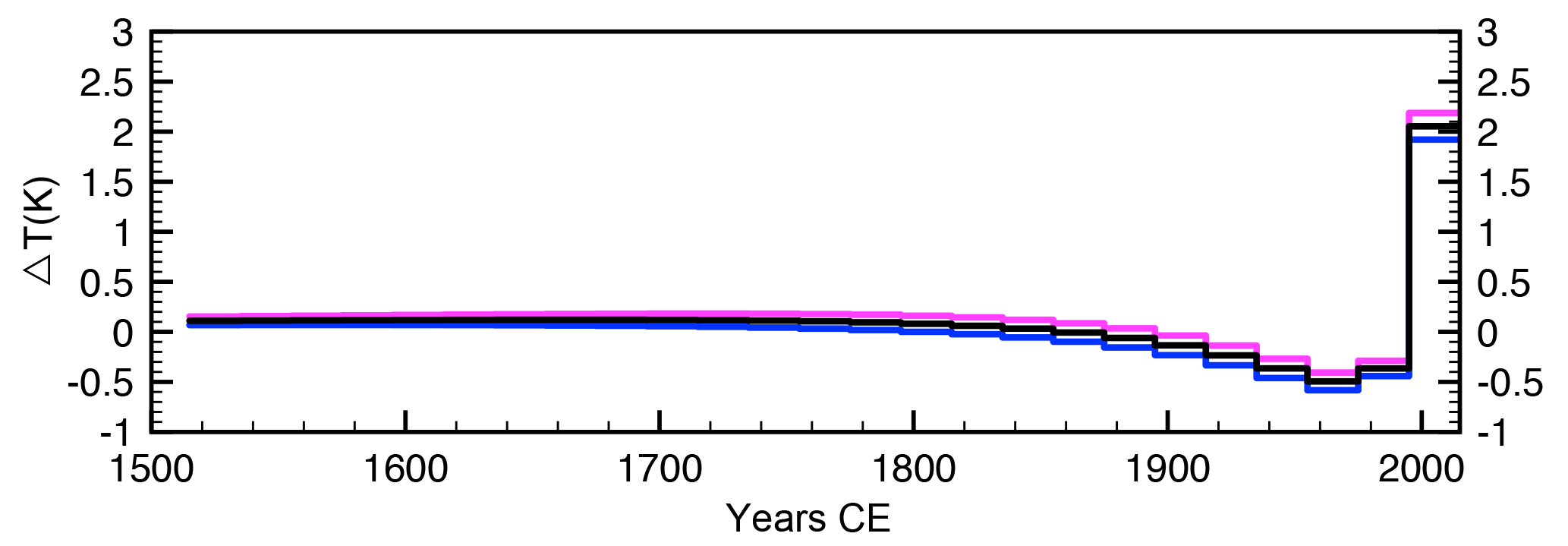
Figure 9 GST history for north-central Chile determined by the simultaneous inversion of DDH2457, 1501, 1504, 1505, RC370, and ala1110-2, with three eigenvalues retained. The pink and blue lines represent the inversion of the upper and lower bounds of the temperature anomaly or the extremal steady states.

4 Inversion results

The GST histories of the past 500 years relative to the measurement date were inverted for the four retained sites (Michilla, Inca de Oro, Totoral, Vallenar). For the inversion the GST history was parameterized by using a model consisting of 25 time-intervals of 20 years with constant temperature (Figs. 5–8). We tried different parameterizations with intervals of varying sizes and found no significant differences among all the inversions. We have carried out individual inversions for each of the retained holes, but we shall only show the results of simultaneous inversions of all the profiles for the sites with multiple boreholes (Michilla and Inca de Oro). The main inferences of the inversions for all the sites are summarized in Table 2. Because we expect meteorological trends to be correlated over distances < 500 km, we have also simultaneously inverted the six borehole temperature–depth profiles from north-central Chile (Fig. 9). For all the inversions, we have used a high singular cutoff value which resulted in retaining only three singular values. This yields a stable solution for the retained singular values which correspond to the long trends, but at the expense of resolution of shorter variations corresponding to lower singular values (Mareschal and Beltrami, 1992).

The GST history of northern coastal Chile (Michilla) shows no warming or cooling for the past 500 years (Fig. 5). The temperature anomalies of the three Michilla profiles show very weak and inconsistent signals (Fig. 4). Two of the temperature anomalies are slightly negative (≈ −0.2 K) indicating a cooling, while the other anomaly is positive and consistent (≈ 0.5 K) with a warming. The small amplitudes of the anomalies and inconsistencies point to the absence of a signal above the level of noise (0.1–0.2 K) and no resolvable change in GST. On visual inspection, these profiles measured with DTS appear very noisy (Figs. 3 and 4) with oscillations of ±0.2 K around the mean trend, which may be due to the poor resolution of the DTS. In such noise, a weak climate signal cannot be resolved. However, we can infer that, for the past 100 years, surface temperature changes cannot exceed 0.5 K. This nul result differs from the trends inferred in north-central Chile. Such a difference is not unlikely since the two regions are over 500 km apart.

In contrast, the profiles in north-central Chile show a negative temperature gradient and a positive temperature anomaly near the surface, indicative of recent warming, followed by a linear increase in temperature with depth. The presence of noise in these data, shown by the irregular variations in temperature gradient, lowers the resolution of the inversion. The temperature anomalies are well marked on all the profiles from Inca de Oro and Totoral; the temperature anomaly at Vallenar is not so well defined because the uppermost 40 m of the profile could not be measured and is missing (Fig. 4). The anomalies suggest that all three sites have experienced warming and that GST is higher now than in the past. This conclusion is supported by the inversion of GST histories for all the sites (Figs. 6–8), but marked differences exist between Totoral on the one hand and Vallenar and Inca de Oro on the other. The warming at Inca de Oro and Vallenar is very recent, beginning after 1960, and appears to follow a long cooling period from 1800 to 1960, while Totoral shows no cooling but warming starting much earlier, ≈ 1800. The amplitude of warming varies from 0.4 K at Vallenar to 2.2 K at Inca de Oro. The maximum temperature is reached at present (2015) for Inca de Oro and Vallenar. However, at Totoral, the maximum temperature, a warming of 1.7 K, was reached in 1980 and was followed by a cooling of ≈ 1 K until present. The robustness of this conclusion is questionable as there is no obvious sign of very recent cooling in the temperature anomaly and it may be a consequence of the limited resolution of the inversion with three singular values. For the sites Inca de Oro and Vallenar, the inversions show a cooling of ≈ 1 K between 1800 and 1980, followed by a strong warming (1.5 K at Inca de Oro and 2.5 K at Vallenar). Cooling followed by warming can also be inferred by visual inspection of the temperature anomalies at these sites. The inversion of the temperature profile at Totoral shows a warming trend by about 2 K between 1800 and present. For Totoral, the cooling is not present in the GST history and no sign of it can be seen in the temperature anomaly.

Despite the differences among the GST inversions of the three sites in north-central Chile, they all show a consistent warming trend. The simultaneous inversion of the six north-central Chile temperature–depth profiles yields a GST history similar to those of Inca de Oro and Vallenar (Fig. 9). There is no warming or cooling between 1500 and ≈ 1800. A cooling of 0.6 K is inferred between ≈ 1800 and 1980, followed by a warming of 1.9 K until present.

5 Discussion

5.1 Comparison with other borehole temperature studies in South America

A recent climate warming of ≈ 0.5–2 K with respect to the long-term GST has been detected for all the sites in north-central Chile. The sites are located in the Atacama Desert, a region with little to no vegetation. In such a region with very low population density and without agriculture, changes in land use are insignificant and could not have generated a fake warming signal. Also, the amplitude of the inferred climate warming is in the range suggested by Huang et al. (2000) for the South American continent (1.4 K) and comparable with the warming of ≈ 1.4–2.2 K starting in the late 19th century inferred for semiarid regions of South America (Hamza and Vieira, 2011). The timing of the warming in the latter study coincides with that of the Totoral site but it is much earlier than the very recent warming (past 40 years) at Inca de Oro, Vallenar, and for the entire north-central Chile region. There is also no evidence of prior cooling in the GST for semiarid South America, suggesting that this cooling episode may be a local feature of north-central Chile. Records from a meteorological station located near the Copiapó airport, which cover only the second half of the 20th century, show a very strong cooling period (−3 K) between 1950 and 1960. This cold period also appears in the CRUTEM4 compilation of meteorological records on a $\mathrm{5}\times \mathrm{5}{}^{\circ }$ grid. The effect of such a cooling event on the inversion of the temperature anomaly will be discussed when we compare our results with meteorological records.

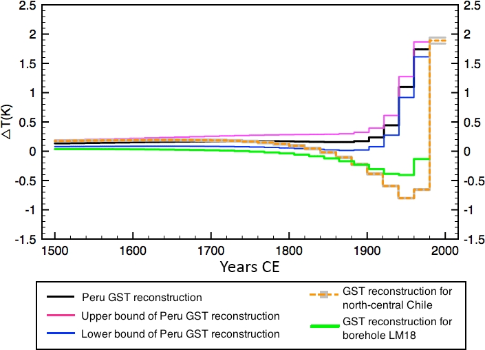
Figure 10 Comparison of GST histories for Peruvian boreholes (black), Peruvian profile LM18 (in green), and north-central Chile (orange) with its upper and lower bounds (grey shaded area). The GST for the Peruvian boreholes was obtained by the simultaneous inversion of LM18 and LOB525 and is relative to the measurement time (1979). Inversion of LM18 shows a cooling similar to that observed in north-central Chile. The inversions of the upper and lower bounds of the temperature anomaly for the Peruvian boreholes are represented by the pink and blue lines, respectively.

Huang et al. (2000) did not include any borehole temperature–depth profiles from northern Chile in their global study, but they analyzed four borehole temperature–depth profiles from the semiarid region of Peru. Only two of these profiles meet our selection criteria (LM18 and LOB525), the other two (LOB527 and PEN742) being too shallow. We have determined the GST history for the selected Peruvian boreholes using simultaneous inversion of the temperature anomalies from the profiles cut at 300 m and retaining three singular values. We then compared the Peruvian and north-central Chile GST histories although they do not cover exactly the same time period (Fig. 10). The GST history of the Peruvian profiles ends in 1979, the year of measurement. Both the Peruvian and the north-central Chile GSTs show no warming or cooling for the period between 1500 and ≈ 1800. Following this period, the Peruvian GST shows warming by 1.6 K until 1979. The amplitude of this warming signal is similar to that of north-central Chile (1.9 K) but it starts much earlier and the simultaneous inversion shows no cooling period. We also inverted each profile individually and we noted that for LM18, the Peruvian site closest to the border with Chile and at the northern edge of the Atacama Desert, a cooling of ≈ 0.5 K is present from ≈ 1800 to 1950, similar to that observed in north-central Chile. We cannot rule out that this apparent cooling is an artifact of the noise and the limited resolution of the inversion; however the similarity of the results suggests that the cooling is real and reflects regional differences in the response of the climate system to warming.

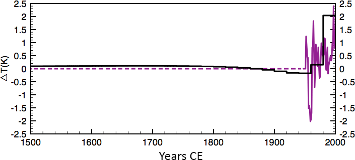
Figure 11 Meteorological record from Copiapó airport (in purple) used as input for calculating a synthetic temperature anomaly and result of its inversion using three singular values (in black). The solid purple line is the actual meteorological record (1950–2014); the dashed horizontal line is an extrapolation of the mean temperature of the record.

5.2 Comparison with meteorological data

In order to compare our results with meteorological records, we have used the worldwide compilation of air surface temperature records on land included in the CRUTEM4 data set (Jones et al., 2012). These records are averaged on a $\mathrm{5}\times \mathrm{5}{}^{\circ }$ grid but we have used the records of individual stations. We have also used the complete meteorological record of the station at Copiapó. For northern coastal Chile, the CRUTEM4 data include stations at Iquique (≈ 260 km north of Michilla), Mejillones (≈ 55 km south of Michilla), and Antofagasta Cerro (≈ 80 km south of Michilla) and cover the period 1900–2016 with very important gaps. There appears to be a marked cooling around 1940, but there are gaps in the data between 1930 and 1960. A warming of ≈ 1 K is observed around 1980. Such warming is inconsistent with the nul result of the GST history inferred for the region. Because the temperature profiles obtained by DTS are quite noisy, we cannot rule out very weak temperature variations (<0.5 K), but our analysis of the temperature profiles suggests no significant climate warming for northern coastal Chile.

In north-central Chile, the CRUTEM4 data include stations at La Serena, Vallenar, Copiapó, and Caldera but cover only the years 1940 to 2016. The mean yearly temperature from all the stations does not show a marked increase over the period, but it does show large amplitude variations including a marked cooling period from 1960 to 1970 similar to that at the Copiapó weather station. After 1970, there is modest warming consistent with but with much less amplitude than the warming in the GST history for this region.

Examination of meteorological data from Copiapó, a city less than 100 km away from Inca de Oro, shows a temperature decrease of ≈ 2.5 K between 1960 and 1970. To determine whether this cooling could be resolved in the GST reconstruction, we have generated a synthetic profile for a cooling of 2.5 K between 1950 and 1960 that we inverted for a GST history of the last 500 years using the same parameters as in the study above (intervals of 20 years, retaining three eigenvalues). The inversion yielded a cooling of 0.5 K between 1800 and 1960, suggesting that a strong cooling event between 1950 and 1960 could appear as the cooling trend in the north-central GST history. This cooling event might explain the long cooling trend preceding a very short and strong warming seen in the GST history for central Chile (Fig. 9). We believe that this result might be an artifact of the lack of resolution of our inversion procedure. With only the three largest singular values retained, the inversion does not resolve short period signals regardless of their strength. That such short period signals might have been present and affected the temperature profiles is suggested by the temperature record at the Copiapó airport meteorological station. This short (1950–present) weather record shows an 8-year interval (1960–1968) with a temperature ≈ 2 K colder than the mean (Fig. 11). We have calculated the perturbation of a 300 m deep temperature profile caused by a surface temperature variation identical to that of Copiapó's weather station and we inverted it retaining only the three largest singular values (Fig. 11). We note that the resulting GST history exhibits a very long trend of decreasing temperature followed by a very sharp increase not dissimilar to the surface temperature history inferred for north-central Chile.

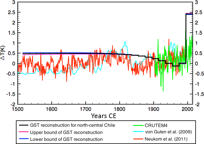
Figure 12 Comparison of GST history for north-central Chile (black) along with the upper and lower bounds of the inversion (pink and blue lines, respectively), the CRUTEM4 data for the north-central Chile grid point (green) (Jones et al., 2012), the austral summer surface air temperature reconstruction from sedimentary pigments for the past 500 years (aqua) at Laguna de Aculeo, central Chile (von Gunten et al., 2009), and the austral summer surface air temperature reconstruction for southern South America (red) with its 2σ standard deviation (grey shaded area) (Neukom et al., 2011). They are all presented as temperature departures from the 1920–1940 mean.

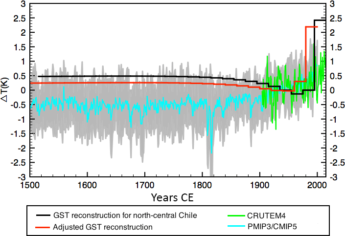
Figure 13 Comparison of two GST histories for north-central Chile (black and red lines) with the CRUTEM4 data for the north-central Chile grid point (Jones et al., 2012), and the multi-model mean surface temperature anomaly reconstruction for the PMIP3-CMIP5 (aqua) with its 2σ standard deviation (grey shaded area). They are all presented as temperature departures from the 1920–1940 mean. The black line is the result of the inversion of all the temperature profiles; the red line is the same adjusted to remove the effect on the inversion of a hypothesized short marked cooling (−2 K) event between 1950 and 1960.

5.3 Comparison with other climate proxies

The north-central Chile GST history was also compared with the linear regression 5-year smoothed austral summer surface air temperature reconstruction from sedimentary pigments at Laguna Aculeo, central Chile (von Gunten et al., 2009), and the southern South America austral summer surface air temperatures inferred from 22 annually resolved predictors from natural and anthropogenic archives (Neukom et al., 2011) (Fig. 12). Although there have been paleoclimatic studies in northern Chile, they do not focus on the recent climate, i.e., the last 1000 years (e.g., Bobst et al., 2001; Grosjean et al., 2003), leading to the comparison with the von Gunten et al. (2009) and Neukom et al. (2011) data. This also provides insight to whether the trends in northern Chile are regional or extend through central Chile and southern South America. From 1500 to 1700, there is no warming or cooling observed in any of the proxy climate reconstructions. Decadal variations, which cannot be resolved in the GST, are observed from 1700 to 1900 in the climate reconstruction for central Chile and southern South America. The climate reconstructions for the three regions show a recent climate warming but differences are noted with respect to the timing of its onset and its amplitude. In southern South America and central Chile, a recent warming of ≈ 0.5 K starting at ≈ 150 years BP is inferred. In northern Chile, the warming begins significantly later, ≈ 20–40 years BP, and reaches a maximum of 1.9 K with respect to the long-term GST. No cooling trend is observed in the central Chile or southern South America climate reconstructions. These differences suggest that there are spatial and temporal variations in climate trends in Chile and southern South America. The cooling and greater-amplitude recent warming are regional features of north-central Chile but the absence of warming or cooling from 1500 to 1700 is a climate trend for southern South America.

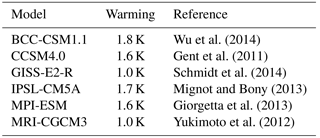
Wu et al. (2014)Gent et al. (2011)Schmidt et al. (2014)Mignot and Bony (2013)Giorgetta et al. (2013)Yukimoto et al. (2012)

Table 3 Summary of models used to calculate the multi-model mean surface temperature anomaly from the PMIP3-CMIP5 simulation.

5.4 Comparison with models

The simulations of the last millennium for the Paleoclimate Modelling Intercomparison Project Phase III (PMIP3) of the Coupled Model Intercomparison Project Phase 5 (CMIP5) provide insight to the climate of the last millennium (Braconnot et al., 2012; Taylor et al., 2012). The six models used to determine the multi-model mean surface temperature anomaly are outlined in Table 3. The multi-model mean surface temperature anomaly from the last millennium PMIP3-CMIP5 simulations for the grid points of northern coastal and north-central Chile show similar trends. Between 1500 and 1900, there is no warming or cooling. From 1900 to present, there is a warming of ≈ 1 K. This supports the absence of climate signal in the GST history of northern coastal Chile. Similarities are observed between the multi-model mean surface temperature anomaly for the north-central Chile grid point and the GST history for the region (Fig. 13). Both infer no warming or cooling between 1500 and ≈ 1800 and a recent warming. The warming of the PMIP3-CMIP5 surface temperature simulation is half and starts earlier than that reconstructed by the GST history. No cooling is observed in the PMIP3-CMIP5 surface temperature simulation for the north-central Chile grid point. This further suggests that this cooling trend and greater-amplitude recent warming are local trends for north-central Chile and cannot be resolved on the PMIP3-CMIP5 grid point scale.

6 Conclusions

We collected and analyzed 31 temperature–depth profiles in north-central and northern Chile but only nine independent profiles were retained for inversion of the ground surface temperature history for the past 500 years.

For northern coastal Chile, the inversion of the temperature–depth profiles shows little or no climate variations (warming or cooling) over the past 500 years.

In north-central Chile, the inversions of six profiles from three different sites yield some consistent conclusions: no warming or cooling can be resolved between 1500 and 1800 for all sites; all sites show recent (< 50 years) and pronounced (0.5–2 K) warming; for two of the sites, some cooling may have preceded this recent warming, but we cannot discriminate between short (10 years) and strong (3 K) cooling episodes and a long cooling trend (150 years).

The amplitude of warming in north-central Chile in consistent with that inferred from other borehole temperature studies in other parts of South America. The warming is greater than that calculated in the PMIP3-CMIP5 surface temperature simulation for the northern coastal and north-central Chile grid points.

A cooling episode is also inferred from the study of one borehole in Peru at the northern edge of the Atacama desert. A short and strong cooling episode is consistent with the CRUTEM4 compilations of meteorological records, but these are unfortunately too short for comparing long-term trends.

Our study suggests the presence of spatial and temporal climate variations in northern Chile, at a scale which cannot be well resolved by the simulations or by the limited data sets available.

Appendix A: Boreholes not suitable for climate

The borehole temperature–depth profiles that did not meet the selection criteria for climate studies are displayed in Fig. A1. The reason for eliminating these holes is given in Table A1. The majority of borehole temperature–depth profiles were rejected because they were deemed too shallow, i.e., they were less than 300 m deep or had no measurements in the top 100 m. This was frequent because measurements above 100 m could not be made when the water table was too deep, and/or because the end of the hole could not be reached in the many holes that had collapsed due to seismic activity. Some profiles were also eliminated due to discontinuities, signs of water flow, or other perturbations through visual inspection of the profiles. Some sites were excluded because of the topography when they are located on or near a steep slope.

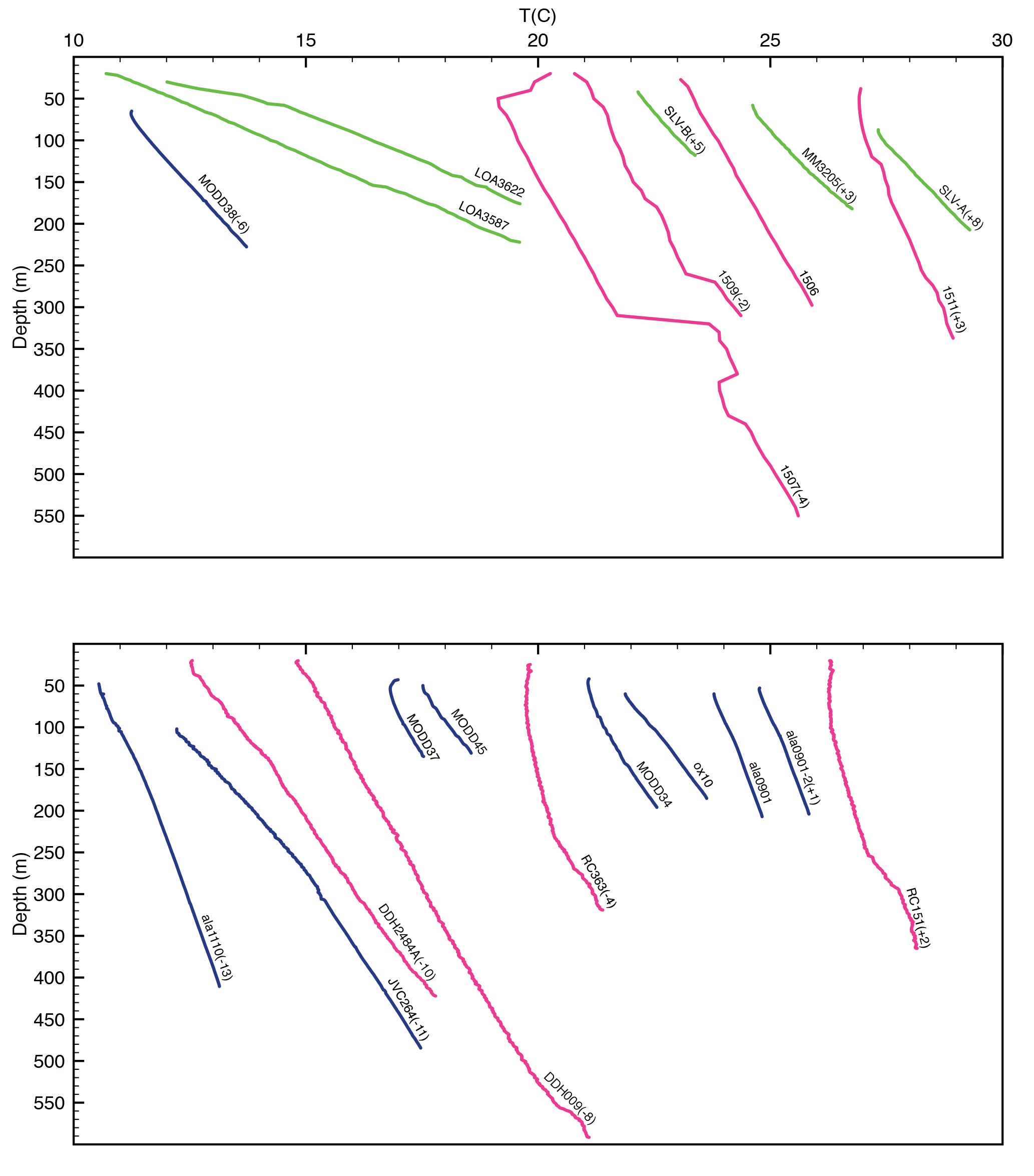
Figure A1 Rejected temperature–depth profiles measured in 1994 (green), 2012 (blue), and 2015 (pink). Temperature scale is shifted as indicated in parentheses.

Springer (1997)Springer and Förster (1998)Springer (1997)Springer and Förster (1998)Springer (1997)Springer and Förster (1998)Gurza Fausto (2014)Gurza Fausto (2014)Gurza Fausto (2014)Gurza Fausto (2014)Springer (1997)Springer and Förster (1998)Springer (1997)Springer and Förster (1998)Gurza Fausto (2014)Gurza Fausto (2014)Gurza Fausto (2014)Gurza Fausto (2014)Gurza Fausto (2014)

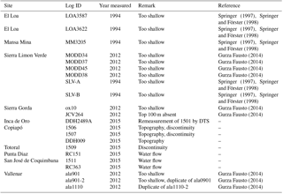
Table A1 Technical information concerning boreholes not suitable for this study.

A1 El Loa

The site is mountainous and includes two boreholes. This is the furthest east and has the highest elevation (3950 m) among all the sites in this report. The lithology of the boreholes is primarily grandiorite and rhyolite (Springer, 1997; Springer and Förster, 1998). The temperature–depth profiles were too shallow for climate studies. They indicated high heat flux in the region (Fig. A1), which could be attributed to the proximity of two volcanoes, the Miño Volcano (≈ 6 km) and the Cerro Aucanquilcha (≈ 20 km).

A2 Mansa Mina

The Mansa Mina borehole is located in a relatively flat region in sediments and granodiorite (Springer, 1997; Springer and Förster, 1998). It is < 10 km from the Chuquicamata open pit mine and ≈ 10 km from the city of Calama. It is too shallow for climate studies.

A3 Sierra Limon Verde

Six borehole temperature–depth profiles were measured in Sierra Limon Verde. They are shallower than 300 m, found within 25 km and sediments make up the main lithology (Springer, 1997; Springer and Förster, 1998). Boreholes MODD37, MODD38, and MODD45 lie on top of a ≈ 400 m high hill. SLV-A and SLV-B are situated on the southern flank of this hill and MODD34 on the northern slope. The site is ≈ 25 km from the city of Calama and ≈ 35 km from the Mansa Mina borehole.

A4 Sierra Gorda

The two boreholes, ≈ 9 km apart, are located in a relatively flat region, close to the Sierra Gorda open pit mine and ≈ 30 km southeast of the village of Sierra Gorda. One hole was too shallow to be retained for climate studies. For the other (JVC2641), the topmost 100 m are missing and the change in the gradient at about 300 m depth is indicative of a change in thermal conductivity.

A5 Vallenar

This site, ≈ 20 km from Vallenar and ≈ 40 km from the coast, has two boreholes that have been measured twice using the same measurement technique. The repeat measurements were not included in order to not bias the reconstructions and only borehole ala1110 was retained for climate studies. The temperature–depth measurement of borehole ala0901 was discarded for being too shallow. Borehole ala0901 is ≈ 300 m from borehole ala1110 and is located between two hills, ≈ 20 km from Vallenar and ≈ 40 km from the coast. This site is about 40 km north of the Vallenar site reported by Uyeda et al. (1978).

A6 Copiapó

Two boreholes, ≈ 200 m apart, were measured ≈ 10 km east of the city of Copiapó. The temperature–depth profile of borehole 1507/DDH009 was measured twice using different techniques, conventional and DTS. The two boreholes were rejected because they are in an area of significant topography. Obviously, the strong discontinuities visible in the profiles of boreholes 1506 and 1507 are sufficient cause to reject them. Water flow is strongly suspected for both holes. An incident occurred during the logging of 1507, when the cable experienced a very strong downward pull that lasted for several seconds, likely caused by a slump of mud within the borehole.

A7 Totoral

The site is in a relatively flat area, ≈ 75 km southwest of Copiapó and ≈ 50 km from the coast. Two temperature–depth profiles for borehole 1509/RC370 were obtained using the conventional method and DTS. The profile obtained using DTS was retained, while that measured using the conventional method showed discontinuities probably caused by instrumental problems and was rejected.

A8 Punta Diaz

The site is on top of a ≈ 100 m hill and ≈ 3 km from the town of Punta Diaz. Signs of water flow are present in the temperature–depth profile, which lead to its exclusion.

A9 San José de Coquimbana

The site is on the side of a small hill, ≈ 40 km from Vallenar and ≈ 30 km from the coast. Using DTS and the conventional method, two temperature–depth profiles were measured for borehole 1511/RC363. Both profiles show signs of water flow and were discarded.