Sedproxy: a forward model for sediment-archived climate proxies

Climate reconstructions based on proxy records recovered from marine sediments, such as alkenone records or geochemical parameters measured on foraminifera, play an important role in our understanding of the climate system. They provide information about the state of the ocean ranging back hundreds to millions of years and form the backbone of paleo-oceanography.

However, there are many sources of uncertainty associated with the signal recovered from sediment-archived proxies. These include seasonal or depth-habitat biases in the recorded signal; a frequency-dependent reduction in the amplitude of the recorded signal due to bioturbation of the sediment; aliasing of high-frequency climate variation onto a nominally annual, decadal, or centennial resolution signal; and additional sample processing and measurement error introduced when the proxy signal is recovered.

Here we present a forward model for sediment-archived proxies that jointly models the above processes so that the magnitude of their separate and combined effects can be investigated. Applications include the interpretation and analysis of uncertainty in existing proxy records, parameter sensitivity analysis to optimize future studies, and the generation of pseudo-proxy records that can be used to test reconstruction methods. We provide examples, such as the simulation of individual foraminifera records, that demonstrate the usefulness of the forward model for paleoclimate studies. The model is implemented as an open-source R package, sedproxy, to which we welcome collaborative contributions. We hope that use of sedproxy will contribute to a better understanding of both the limitations and potential of marine sediment proxies to inform researchers about earth's past climate.

1 Introduction

Climate proxies are an imperfect record of the earth's past climate. Climate variations are encoded by geo- or bio-chemical processes into a medium which survives, archived, until it is sampled and the physical or chemical signal decoded back into estimates of direct climate variables. For example, the ratio of magnesium to calcium in the shells (tests) of foraminifera varies with the water temperature at which they calcify and thus encodes a temperature signal (Nürnberg et al., 1996). Upon death, these shells (the carrier) become buried (archived) in the sediment. They can later be recovered from sediment cores and their Mg∕Ca ratio measured. Using the modern-day relationship between foraminiferal Mg∕Ca and temperature, down-core variations in the Mg∕Ca ratio in foraminiferal tests can then be decoded back into an estimate of temperature variations back in time (Anand et al., 2003; Barker et al., 2005; Elderfield and Ganssen, 2000).

The climate signal is distorted and obscured at many points during the encoding, archiving, and subsequent reading of a climate proxy, and these diverse sources of noise and error need to be taken into account when estimating the true past climate from proxy records. One way to develop, test, and improve our ability to reconstruct climate from proxies is to create mechanistic forward models. These models attempt to simulate the key processes on the entire path from the climate signal to the reconstructed climate: from the encoding of the signal; its archiving in, for example, ice, sediments, wood, or coral; recovery of the archived material; cleaning and processing of samples; measurement of the physical or chemical proxy; and its conversion back into a climate variable such as temperature. Models that attempt to cover this entire process are known as proxy system models (PSMs; Evans et al., 2013) and detailed PSMs have recently been proposed and implemented for oxygen isotope proxies archived in ice, trees, speleothems, and corals (Dee et al., 2015).

Climate proxies recovered from sediment cores are widely used to reconstruct past climate evolution on timescales from centuries (Black et al., 2007) up to millions of years (Zachos et al., 2001). Several processes affecting the climate signal during recording, recovery, and measurement have been described in the literature and analysed in specific studies. Examples include the influence of seasonal recording (Leduc et al., 2010; Lohmann et al., 2013; Schneider et al., 2010), the effect of bioturbation (Berger and Heath, 1968; Goreau, 1980), the sample size of foraminifera (Killingley et al., 1981; Schiffelbein and Hills, 1984), measurement uncertainty (Greaves et al., 2008; Rosell-Melé et al., 2001), and inter-test variability (Sadekov et al., 2008). Despite this body of knowledge, in practice these processes are often considered only in isolation, or not at all, when marine proxy records are interpreted, or when model–data comparisons are made.

The R package sedproxy provides a forward model for sediment-archived climate proxies so that the above processes can be considered during study design, the interpretation of marine proxy records, and when comparing models with data. Sedproxy is based on and expands the model described and used by Laepple and Huybers (2013) to explain differences in variance between alkenone (U${}_{\mathrm{37}}^{{\mathrm{K}}^{\prime }}$) and Mg∕Ca-based climate reconstructions. We first give an overview of the stages of sedimentary proxy record creation and then describe how these are implemented in sedproxy. We then demonstrate how to use the package with a diverse series of use cases. The source code for sedproxy is available from the public git repository https://github.com/EarthSystemDiagnostics/sedproxy. A snapshot of the version used here is archived on Zenodo (Dolman and Laepple, 2018).

2 Creation of sediment-archived proxy records

The creation of a proxy climate record can be thought of as having three stages: sensor, archive, and observation (Evans et al., 2013). Here we describe, for sediment-archived proxy records, the key processes that occur in each of these stages and outline which of these are included in sedproxy.

2.1 Sensor stage

In the context of a climate proxy, a sensor is a physical, biological, or chemical process that is sensitive to climate (e.g. temperature), and creates a measurable record of the climate signal. For example, the widths of tree growth rings are sensitive to temperature and water availability and are preserved in tree trunks (Douglass, 1919). Our forward model can be used for any proxy sensor that records water conditions and is then deposited and archived in the sediment. We consider here, as examples, two climate sensors: the Mg∕Ca ratio in the tests of foraminifera, and the alkenone unsaturation index (U${}_{\mathrm{37}}^{{\mathrm{K}}^{\prime }}$). Foraminifera are single-celled protozoa that exude a calcite shell (test) in which a certain proportion of the calcium ions are substituted for magnesium. The ratio of Mg to Ca ions is dependent on the ambient temperature during the process of calcite formation, and thus the Mg∕Ca ratio in foraminiferal tests acts as a proxy for temperature during their creation (Nürnberg et al., 1996). Similarly, alkenones are a class of large organic molecules synthesized by some Haptophyte phytoplankton species. The proportion of unsaturated carbon to carbon bonds in the synthesized molecules is temperature dependent and thus the relative unsaturation of alkenone molecules found in sediments can be used as a proxy for temperature (Prahl and Wakeham, 1987). Secondary effects such as the effect of salinity on the Mg∕Ca of foraminifera (Hönisch et al., 2013), or nutrient availability on the U${}_{\mathrm{37}}^{{\mathrm{K}}^{\prime }}$ recorded by the alkenone producers (Conte et al., 1998), might further effect the recorded proxy signal.

2.1.1 Seasonal and habitat bias in the sensor

One source of uncertainty common to most climate proxies is a bias towards recording the climate during periods of the year when the proxy generating process is most active (Mix, 1987). Both the foraminifera and the alkenone producing haptophytes have growth rates, abundances and rates of export to the sediment that vary predictably throughout the year (Jonkers and Kučera, 2015; Leduc et al., 2010; Uitz et al., 2010), and hence bias these proxies towards recording the climate during their respective periods of peak production and export. Furthermore, the proxy creating organisms do not necessarily live at and record the surface of the ocean. The producers of alkenones are restricted to the photic zone and thus are close to the surface; however, for foraminifera, the preferred habitat depth and the depth at which their shells calcify is strongly species dependent and can vary from being close to the surface to the thermocline or deeper (Fairbanks and Wiebe, 1980; Kretschmer et al., 2018). Therefore, the recorded temperature will not necessarily reflect the sea surface temperature (SST) (Jonkers and Kučera, 2017). Whether or not these biases represents an error will depend on how the resulting proxy record is interpreted. However, even when a proxy is interpreted as representing a particular season or depth habitat, the season and depth that a given proxy represents will rarely be known with certainty. Furthermore, it is likely that the seasonal and depth-habitat preferences of proxy-producing organisms will respond to changes in the climate, i.e. they will show homeostasis or habitat tracking (Jonkers and Kučera, 2017; Mix, 1987), which will likely damp the climate variations in proxy records (Fraile et al., 2009).

2.2 Archive stage

After the creation of proxy carriers such as foraminiferal shells or alkenone molecules, a proportion of these are exported to and buried in the sediment. The upper few centimetres of marine sediments are typically mixed by burrowing organisms down to a depth of around 2–15 cm (Boudreau, 1998) (Teal et al., 2010; Trauth et al., 1997), although laminated sediments absent of bioturbation do exist. Marine sediment accumulation rates vary over many orders of magnitude (Sadler, 1999; Sommerfield, 2006) but rates at core locations used for climate reconstructions are typically of the order of 1–100 cm kyr⁻¹. Thus, bioturbation can mix and smooth the climate signal over a period of decades to millennia and have a strong effect on the effective temporal resolution that can be recovered from a sediment-archived proxy (Anderson, 2001; Goreau, 1980).

Other processes occurring during the archive stage may influence the proxy, e.g. differential dissolution of Mg∕Ca in foraminiferal shells (Barker et al., 2007; Mekik et al., 2007; Rosenthal and Lohmann, 2002) and preferential degradation of U${}_{\mathrm{37}}^{{\mathrm{K}}^{\prime }}$ (Conte et al., 2006; Hoefs et al., 1998).

2.3 Observation stage

During the observation phase, samples of sediment are taken at intervals along a core and material is recovered in which the proxy signal has been encoded. For U${}_{\mathrm{37}}^{{\mathrm{K}}^{\prime }}$ extraction and foraminifera picking, these samples are typically taken from 1 to 2 cm thick sediment layers. Therefore, even in the absence of bioturbation the proxy record will be smoothed by a time period determined by the sedimentation rate and layer thickness.

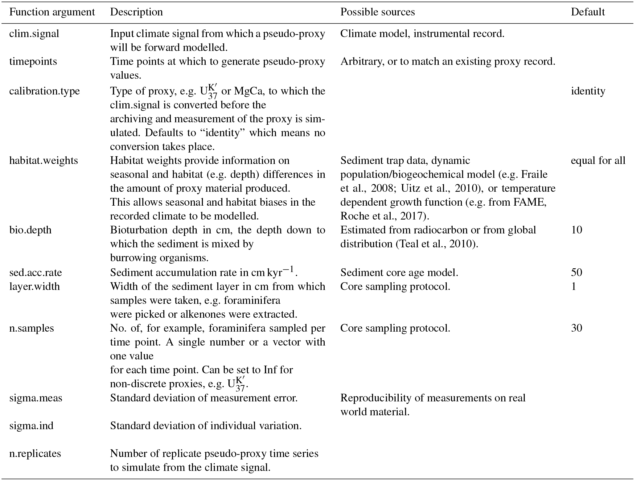
Table 1 Required input data and parameters to generate a pseudo-proxy record with sedproxy. The final argument controls the experimental design rather than the proxy record creation process itself.

2.3.1 Aliasing of inter- and intra-annual climate variation

For proxy signals embedded in the tests of foraminifera, measurements are typically made on relatively small samples of about 5–30 individuals. Due to both bioturbation and the width of the sampled sediment layer, these individuals will be a mixed sample that integrate the climate signal over an extended time period; however, individual planktonic foraminifera live for a period of only 2–4 weeks (Bijma et al., 1990; Spero, 1998) and hence each encodes climate at an approximately monthly resolution. Therefore, if a measurement is made on a sample containing 30 individuals mixed together from a period of 100 years, the resulting value is a noisy 100-year mean and hence inter- and intra-annual scale climate variation is aliased into the nominally centennial-resolution proxy record (Laepple and Huybers, 2013; Schiffelbein and Hills, 1984). This effect may be particularly strong for high-latitude cores where the seasonal temperature cycle is large. However, the stronger the seasonal climate cycle, the more likely an organism is to grow preferentially during a specific season (Jonkers and Kučera, 2015), and thus aliasing will be reduced, while seasonal bias is increased. For organic proxies such as U${}_{\mathrm{37}}^{{\mathrm{K}}^{\prime }}$, samples comprise many thousands of molecules and aliasing is likely a minor issue, although clustering in sediment export and distribution is possible (Wörmer et al., 2014).

2.3.2 Other non-climate variability: inter-individual variation, cleaning and processing, and instrumental error.

The measurement of proxy values on material recovered from sediment cores will necessarily involve some amount of error. In particular, foraminiferal tests need to be cleaned prior to Mg∕Ca measurements and this is an imprecise process. Too little cleaning risks leaving Mg-rich mineral phases (Barker et al., 2003), too much may bias the Mg∕Ca downwards. Some cleaning, processing, and measurement errors will be independent between samples while others may be correlated, e.g. due to differences between labs (Greaves et al., 2008). In addition to measurement error, there will also be inter-individual variation between foraminifera in their recording of the same climate signal (Haarmann et al., 2011; Sadekov et al., 2008). For example, test Mg∕Ca ratios vary between individual foraminifera even when grown under identical conditions (Dueñas-Bohórquez et al., 2011). Similar inter-individual variation and “vital effects” also occur for δ¹⁸O (Duplessy et al., 1970; Schiffelbein and Hills, 1984).

3 Implementation

Here we give an overview of the model implementation, describing which features of proxy creation can be simulated with sedproxy. The essential input data, variables, and parameters are listed in Table 1 and described in the following paragraphs. Additional optional function arguments are described in the sedproxy package documentation.

3.1 Input climate matrix (clim.signal)

Sedproxy takes as input an assumed “true” climate signal, which may come from a climate model or instrumental readings, and returns a simulated proxy value for each of a set of requested time points. The input climate signal is required as a matrix C_y,h where “y” rows are the years and the “h” columns resolve the habitats being modelled. For example, to model seasonal biases in the recording process and noise aliased from monthly climate variation, there should be 12 columns representing 12 months of the year. To include other habitat effects, e.g. foraminiferal depth habitats, this matrix can be extended to have, for example, 12×z columns, where z is the number of discrete depths to be included.

$$\left(\begin{array}{cccc}{\mathbf{C}}_{{\mathrm{y}}_{\mathrm{1}},{\mathrm{h}}_{\mathrm{1}}}& {\mathbf{C}}_{{\mathrm{y}}_{\mathrm{1}},{\mathrm{h}}_{\mathrm{2}}}& \mathrm{\cdots }& {\mathbf{C}}_{{{\mathrm{y}}_{\mathrm{1}},\mathrm{h}}_{\mathrm{12}z}}\\ {\mathbf{C}}_{{\mathrm{y}}_{\mathrm{2}},{\mathrm{h}}_{\mathrm{1}}}& {\mathbf{C}}_{{\mathrm{y}}_{\mathrm{2}},{\mathrm{h}}_{\mathrm{2}}}& \mathrm{\cdots }& {\mathbf{C}}_{{{\mathrm{y}}_{\mathrm{2}},\mathrm{h}}_{\mathrm{12}z}}\\ \mathrm{⋮}& \mathrm{⋮}& \mathrm{\ddots }& \mathrm{⋮}\\ {\mathbf{C}}_{{\mathrm{y}}_n,{\mathrm{h}}_{\mathrm{1}}}& {\mathbf{C}}_{{\mathrm{y}}_n,{\mathrm{h}}_{\mathrm{2}}}& \mathrm{\cdots }& {\mathbf{C}}_{{\mathrm{y}}_n,{\mathrm{h}}_{\mathrm{12}z}}\end{array}\right)$$

3.2 Sensor-model and calibration

The input climate signal can be converted to proxy units using a transfer function based on an established temperature calibration. If the argument calibration.type is set to either “Uk37” or “MgCa”, the input climate matrix will be converted using the global U${}_{\mathrm{37}}^{{\mathrm{K}}^{\prime }}$ to temperature calibration from Müller et al. (1998), or the multi-species Mg∕Ca to temperature calibrations from Anand et al. (2003), respectively. The argument calibration can be used to specify one of the taxon-specific calibrations from Anand et al. (2003). If calibration.type is left at its default value of “identity”, then no transformation takes place. This gives the option for the input climate matrix to be pre-transformed into any proxy type by the user.

Uncertainty in the relationship between temperature and proxy units can be modelled by requesting multiple replicate pseudo-proxies. For each replicate, a random set of calibration parameters are drawn from a bivariate normal distribution that represents the uncertainty in the fitted calibration model. The bivariate distributions are parameterized by mean values for the regression coefficients and corresponding variance-covariance matrices. We have estimated these variance-covariance matrices for the supplied calibrations by refitting regression models to the calibration data used in the original publications. Due to small differences in the data sets and methods, our parameter estimates deviated slightly from the published values, but for consistency the mean parameter values are set to the published values.

As sedproxy does not explicitly model the differential dissolution of foram tests, nor the preferential degradation of U${}_{\mathrm{37}}^{{\mathrm{K}}^{\prime }}$, the implicit assumption is made that, where used, these effect are either minimal or otherwise corrected for during sample processing (e.g. by exclusion of extensively dissolved foram tests). Where a bias due to differential dissolution can be estimated, this could be corrected for using a custom dissolution-correcting temperature calibration (Mekik et al., 2007; Rosenthal and Lohmann, 2002).

Both the Mg∕Ca and U${}_{\mathrm{37}}^{{\mathrm{K}}^{\prime }}$ calibration functions will accept optional arguments that replace their default parameter values and variance-covariance matrices. For alternative calibration models that have a different functional form, the function ProxyConversion would need to be modified.

3.3 Weights matrix

While sedproxy conceptually modifies the climate signal according to a sequence of sensor, archive, and observation processes, in practice the value of the simulated proxy at a given time point is calculated in a single step as the mean of a weighted sample from the original climate signal, plus some independent error term. For each requested time point, a matrix of weights, W_y,h, is constructed which determines the probability of sampling any particular value from the climate matrix.

The elements of the weights matrix W_y,h are the product of annual weights, w_y, which depend on bioturbation, and either a vector or matrix of habitat weights, w_h or w_y,h, corresponding to “static” or “dynamic” habitat weights, respectively. Static weights correspond to habitat preferences (e.g. depth or season) that do not vary over time with climate. Dynamic weights correspond to season and habitat preferences that change in response to climate – such as might be expected from organisms adapting to changing water temperatures by altering their depth in the water column or the timing of their production.

3.3.1 Habitat weights (habitat.weights)

Static habitat weights, w_h, are given by a user-defined vector defining the seasonality and potentially the depth habitat of the proxy recording process. It has the same length as the number of columns in the input climate signal. Dynamic habitat weights can be specified either by passing a named function that will calculate these weights from the input climate matrix or by passing a precalculated matrix of weights of the same size as the input climate matrix. Non-static habitat weights could be generated using either the simple Gaussian response approach of Mix (1987) or something more advanced such as the proposed FAME module (Roche et al., 2018). Sedproxy includes an R implementation of the growth_rate_l09 function from the FAME v1.0 Python module (Roche et al., 2018) that can be used to predict habitat weights from water temperatures for several foraminifera taxa. More complex models, such as FORAMCLIM (Lombard et al., 2011) or PLAFOM (Fraile et al., 2008), could also be used outside of R to precalculate the weights matrix.

Figure 1 The origin of material archived at a focal core depth of 50 cm. In this example the bioturbation depth is 10 cm, and the sediment accumulation rate is 50 cm kyr⁻¹.

There is considerable potential for lateral transport of proxy carriers, particularly the organic proxies such as U${}_{\mathrm{37}}^{{\mathrm{K}}^{\prime }}$ (Benthien and Müller, 2000; Mollenhauer et al., 2003) and potentially also foraminifera (van Sebille et al., 2015); so that proxy material in a given sediment core may have come from a different location or be a mixed sample representing an area of ocean of considerable size. Lateral transport of proxy material in the water column or at the sediment surface could be modelled by using an input climate matrix with columns for multiple spatial locations, and habitat weights representing the probability that material was transported from a given location.

3.3.2 Annual weights (bioturbation)

For simplicity, sedproxy assumes complete mixing within the bioturbated layer, a constant sedimentation rate in the region of each sampled time point, and a constant concentration of the proxy carrying material. Under these assumptions, the origin (pre-bioturbation) of material recovered from a given focal depth is described by the impulse response function Eq. (1) (Berger and Heath, 1968). This function is equivalent to an exponential probability density function, with mean equal to the focal depth and standard deviation equal to the bioturbation depth divided by the sedimentation rate. The value of a proxy measured on material recovered from a given depth can thus be viewed as a weighted mean of material originally deposited over a range of depths, with weights given by Eq. (1) (Fig. 1). By assuming a locally constant sediment accumulation rate, α, around each focal point, and a fixed bioturbation depth, δ, the bioturbation function can be expressed in units of time rather than space or depth.

In this model, the probability that a particle found at a given focal depth was mixed down from a distance greater than the bioturbation depth, δ, is zero. Theoretically, particles can be brought up from any distance below the focal depth, but for computational reasons the annual weights vector is restricted to a distance of three bioturbation depths below the focal horizon; this region contains 99 % of the mass of the impulse response function.

$$\begin{array}{}\text{(1)}& w{y}_t=\left\{\begin{array}{ll}\frac{\mathit{\alpha }\cdot e^{\mathit{\lambda }{y}_{\mathrm{f}}-\mathit{\lambda }{y}_t-\mathrm{1}}}{\mathit{\delta }}& \text{if }{y}_t-y_{\mathrm{f}}+\frac{\mathit{\delta }}{\mathit{\alpha }}\ge \mathrm{0},\\ \mathrm{0}& \text{if }{y}_t-y_{\mathrm{f}}+\frac{\mathit{\delta }}{\mathit{\alpha }}<\mathrm{0},\end{array}\right.\end{array}$$

where α is sediment accumulation rate in cm yr⁻¹, δ is the bioturbation depth in cm, λ is the $\frac{\mathit{\alpha }}{\mathit{\delta }}$, and y_f os the focal year.

To account for the fact that foraminiferal tests are collected, or U${}_{\mathrm{37}}^{{\mathrm{K}}^{\prime }}$ extracted, from a layer of sediment of a certain thickness (layer.width). The bioturbation function is convolved with a uniform probability density function with a width equal to the layer thickness (Eq. 2). The effect of layer.width is small unless the bioturbation depth is small relative to the layer width.

$$\begin{array}{}\text{(2)}& w{y}_t=\left\{\begin{array}{ll}\mathrm{0}& \text{if }z<-L,\\ \frac{e^{-\mathit{\lambda }L-\mathit{\lambda }z}\cdot \left(e^{\mathit{\lambda }L+\mathit{\lambda }z}-\mathrm{1}\right)}{\mathrm{2}L}& \text{if }-L\le z\le L,\\ \frac{\left(e^{\mathrm{2}\mathit{\lambda }L}-\mathrm{1}\right)\cdot e^{-\mathit{\lambda }L-\mathit{\lambda }z}}{\mathrm{2}L}& \text{if }z>L,\end{array}\right.\end{array}$$

where z =$y_t-y_{\mathrm{f}}+\frac{\mathit{\delta }}{\mathit{\alpha }}$ and L =$\mathrm{layer}.\mathrm{width}/\mathrm{2}$.

While the assumption of complete mixing with a sharp cutoff is unlikely to be true, the general effects of bioturbation should also apply under conditions of incomplete mixing and the code could be modified to use a more complex bioturbation model (Guinasso and Schink, 1975; Steiner et al., 2016). However, when sedimentation rates are low relative to mixing rates, more complex mixing models converge to the simple box-type model that is employed here (Matisoff, 1982). Sedproxy further assumes a constant bioturbation depth over time, as the bioturbation depth is generally not known for each setting and cannot easily be reconstructed down-core. Bioturbation depth may be related to productivity and sedimentation rate, but its predictability for a given core seems to be low (Trauth et al., 1997). The recent development of radiocarbon measurements on small samples (Wacker et al., 2010) might allow the extent of bioturbation to be constrained using replicate measurements from individual depth layers (Lougheed et al., 2018) and such information could be included in sedproxy in the future.

3.3.3 Summing or sampling

For proxies such as foraminiferal Mg∕Ca, where typically a small number of foraminiferal tests (N) are cleaned and measured for each depth or time point in a sediment core, the proxy at time t, Pr_t, is the mean of a random sample of N elements of the input climate matrix C, with the probability that a particular element is sampled given by the weights matrix W, plus some independent error term ε (Eq. 3).

$$\begin{array}{}\text{(3)}& {\mathrm{Pr}}_t={\displaystyle \frac{\mathrm{1}}{N}}\sum _{i=\mathrm{1}}^{i=N}\mathit{\{}{\mathbf{C}}^{\left(i\right)},{\mathbf{W}}^{\left(i\right)}\mathit{\}}+\mathit{\epsilon }\end{array}$$

For proxies such as U${}_{\mathrm{37}}^{{\mathrm{K}}^{\prime }}$, it is assumed that there are effectively infinite samples taken for each time point at which the proxy is evaluated. In this case the proxy at time y Pr_t is the sum of the element-wise product of the climate and weights matrices (Eq. 4).

$$\begin{array}{}\text{(4)}& {\mathrm{Pr}}_t=\sum (\mathbf{C}\cdot \mathbf{W})+\mathit{\epsilon }\end{array}$$

3.4 Independent error (sigma.meas, sigma.ind)

The error term ε is added as an independent Gaussian random variable with mean μ = 0 and standard deviation σ. The value of σ is controlled by the parameters sigma.meas (σ_meas), and sigma.ind (σ_ind); σ_meas describes both the analytical error of the measurement process and any other sources of error that are introduced during the preparation of the sample (e.g. cleaning for Mg∕Ca); σ_ind quantifies inter-individual variation for proxies that are measured on samples of discrete individuals such as foraminifera, and its contribution to ε is scaled by the square root of the number of individuals in the sample, N (Eq. 5).

$$\begin{array}{}\text{(5)}& \mathit{\sigma }=\sqrt{{\mathit{\sigma }}_{\mathrm{meas}}^{\mathrm{2}}+{\displaystyle \frac{{\mathit{\sigma }}_{\mathrm{ind}}^{\mathrm{2}}}{N}}}\end{array}$$

Appropriate values for these error parameters will depend on the proxy type, and for σ_ind in particular they may also be site and species dependent, although the empirical estimates of the sum of both error terms in Laepple and Huybers (2013) suggested similar values between study sites. We propose that σ_meas should be set to typical lab values for the reproducibility of measurements on real-world material. For U${}_{\mathrm{37}}^{{\mathrm{K}}^{\prime }}$ we use a value of 0.23 ^∘C, which was the mean replicate error of all U${}_{\mathrm{37}}^{{\mathrm{K}}^{\prime }}$ studies used in Laepple and Huybers (2013). For foraminiferal Mg∕Ca we use 0.26 ^∘C for σ_meas, which corresponds to about 0.07–0.11 mmol mol⁻¹ at 20 and 25 ^∘C, respectively, and lies within the typical reported range (Groeneveld et al., 2014; Skinner and Elderfield, 2005).

The value of σ_ind is less constrained as it depends on how much of this variation has been explicitly modelled, e.g. via a seasonally and depth-resolved input climate signal and habitat weights. We use 2 ^∘C for σ_ind, as most examples here do not explicitly include depth habitat. This value is similar to the inter-test variability of approximately 1.6 ^∘C estimated for fresh Globigerinoides ruber samples by Sadekov et al. (2008). Assuming a typical number of 30 foraminifera individuals per sample, these two sources add up to approximately 0.45 ^∘C, the mean replicate error across all Mg∕Ca studies used in Laepple and Huybers (2013). For U${}_{\mathrm{37}}^{{\mathrm{K}}^{\prime }}$ we set σ_ind to zero as we typically assume an infinite sample size.

Values of σ_meas and σ_ind are entered in units of ^∘C by default, but can be entered in proxy units if scale.noise is set to FALSE.

3.5 Replication

Multiple replicate proxy records can be simulated with a single set of parameters. Due to the stochastic sampling of habitats and depths, the random noise terms, and the randomly sampled calibration parameters, replicates will not be identical. An additional random bias can be added to each replicate-simulated proxy record. This bias is drawn from a Gaussian distribution with mean equal to 0 and a user-definable standard deviation (meas.bias defaults to 0). This bias will be constant for all points in a given replicate and can be used to include additional uncertainty in the proxy calibration, or inter-lab variation in analytical results.

Table 2 Details for sediment core MD97-2141.

4 Using sedproxy

To illustrate the use of sedproxy, we here provide a number of examples together with the R code to execute them.

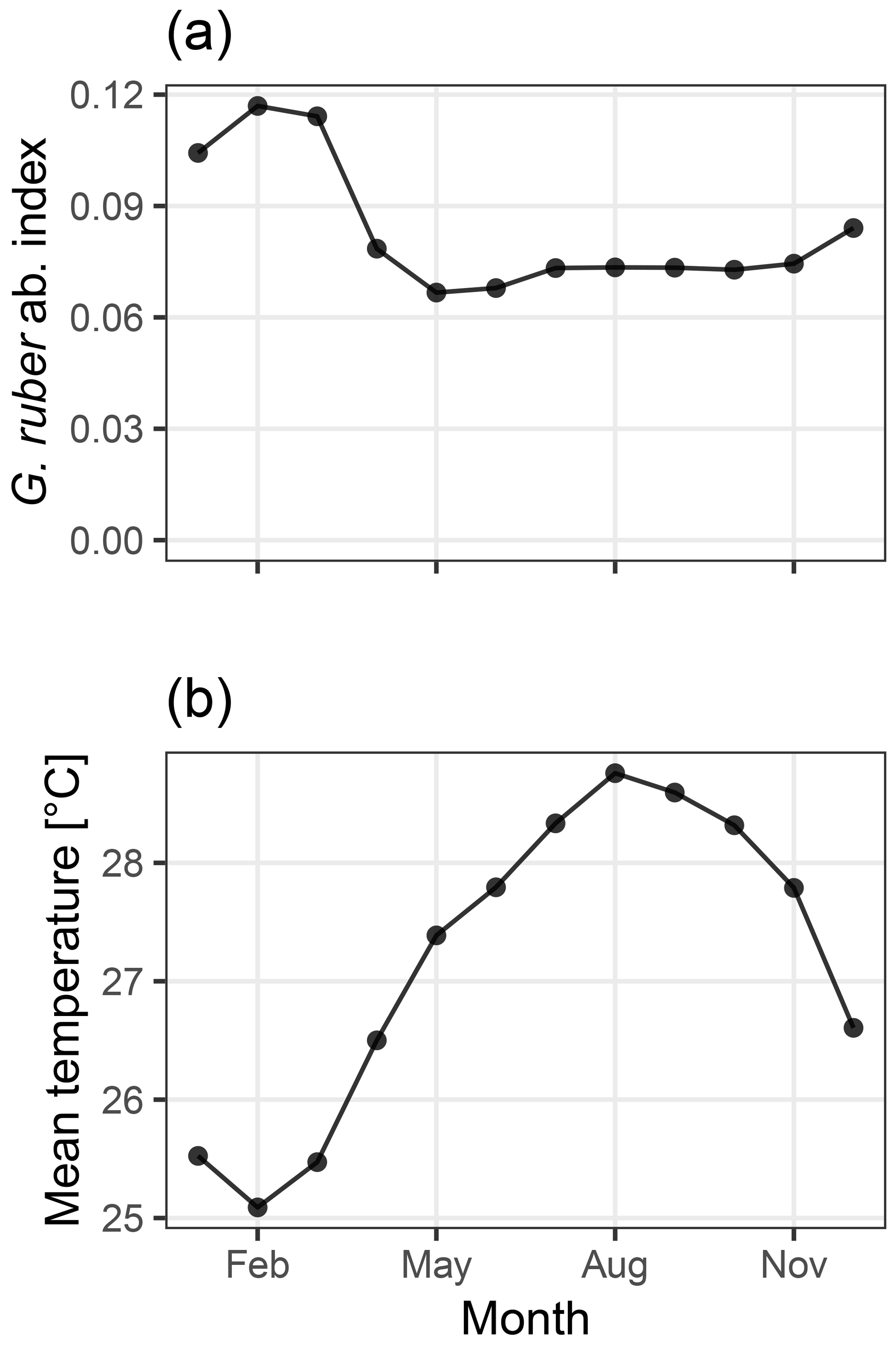
Figure 2 Abundance index of G. ruber from PLAFOM (Fraile et al., 2008) (a), and the mean monthly sea surface temperature in the TraCE21ka simulation at MD97-2141 (b). In this model, G. ruber occurs over the whole year with a small maximum during the cooler months of January–March, therefore biasing the recorded temperature towards colder temperatures.

4.1 Example 1: a foraminiferal Mg∕Ca pseudo-proxy record for sediment core MD97-2141

In this first example, we demonstrate how to simulate an already measured proxy record as closely as possible. We use the foraminiferal Mg∕Ca-based temperature reconstruction for sediment core MD97-2141 (Table 2) in the Sulu Sea (Rosenthal et al., 2003).

As an input climate signal we take the monthly SST output from the TraCE-21ka “Simulation of Transient Climate Evolution over the last 21 000 years” (Liu et al., 2009), using the grid cell closest to core MD97-2141.

We use an Mg∕Ca calibration with user-supplied mean values for the slope and intercept set to those used by Rosenthal et al. (2003) which reduce a bias due to partial dissolution. The seasonality of Globigerinoides ruber, the foraminifera for which test Mg∕Ca ratios were measured, is taken from the dynamic population model PLAFOM, driven with modern climatology (Fraile et al., 2008; Fig. 2a). Sediment accumulation rates were estimated from the depth and age data associated with core MD97-2141 and provided in the Supplement to Shakun et al. (2012). These data are included in the sedproxy R package as example data and are also used in the later examples.

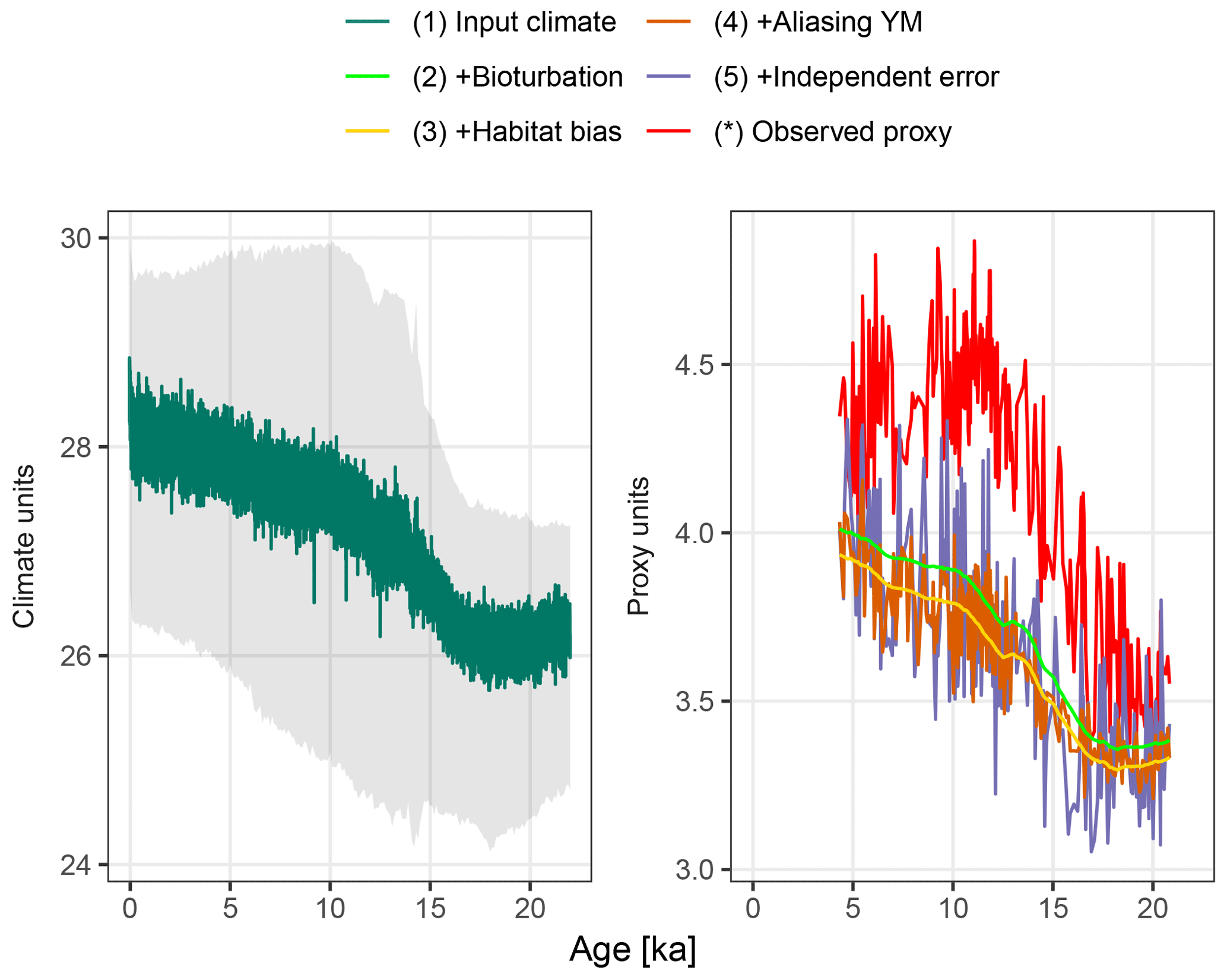
Figure 3 A forward modelled foraminiferal Mg∕Ca pseudo-proxy record together with the observed Mg∕Ca proxy record at core MD97-2141 in the Sulu Sea. The input climate is shown at annual resolution with the full monthly input time series in grey.

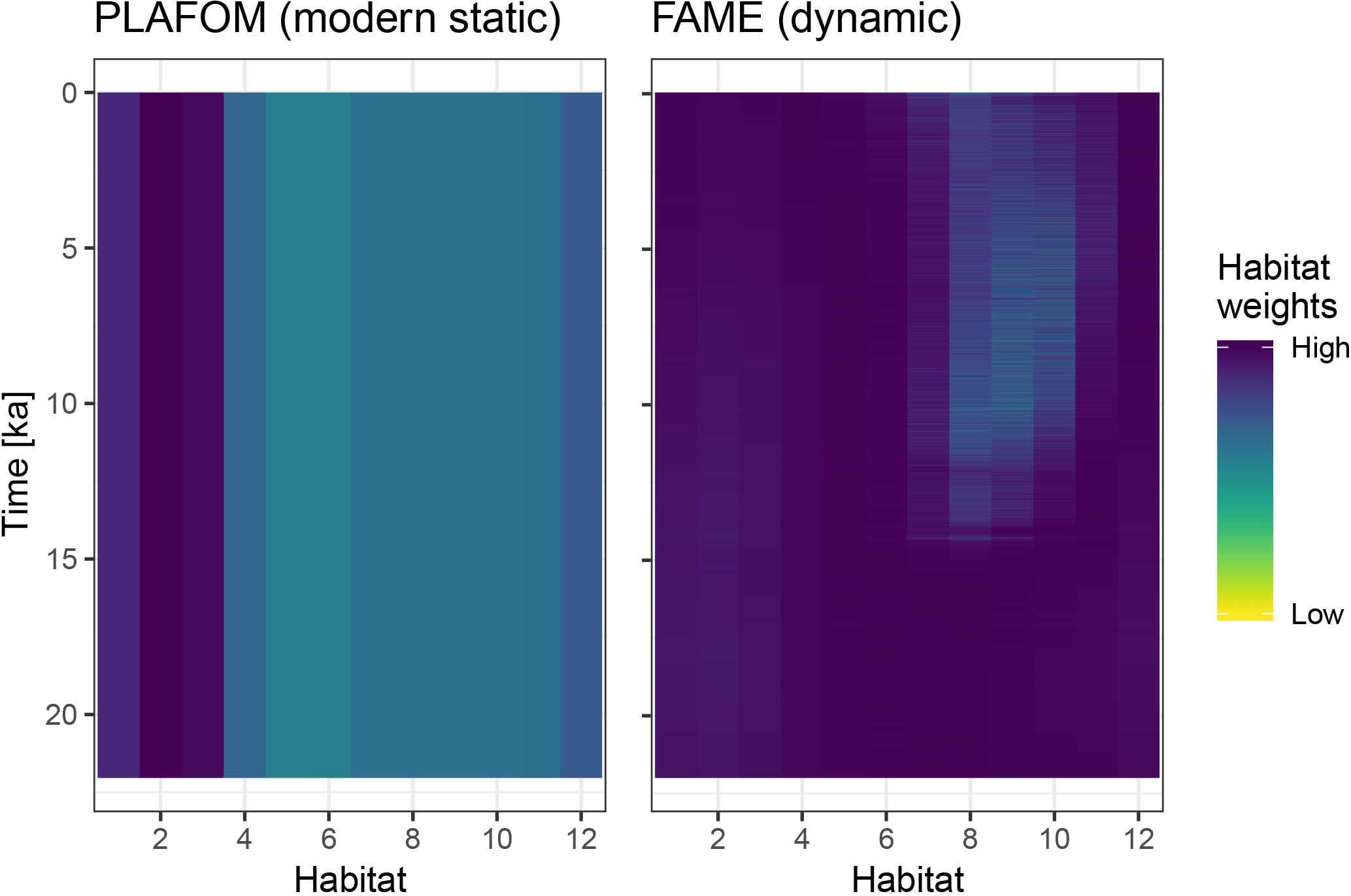
Figure 4 A comparison of static and dynamic monthly weights generated by PLAFOM driven by modern climatology, and FAME driven by the input climate matrix.

The function ClimToProxyClim is used to forward model a proxy record from an assumed climate. We request values of the proxy at the time points of the observed proxy. Descriptions of the main function arguments can be found in Table 1, other optional arguments are described in the package documentation. From the R console type ?ClimToProxyClim to see the help page.

library(sedproxy)

# Reverse matrix so that top row is most recent
# year, also convert from Kelvin to Â∘C
n.rows <- nrow(N41.t21k.climate)
N41.t21k.climate.in <-
N41.t21k.climate[n.rows:1, ] - 273.15

# Convert matrix to a ts object and set start to
# most recent year, in this case -39
# (1989 in years "before" 1950)
N41.t21k.climate.in <-
  ts(N41.t21k.climate.in, start = -39)

# Set seed of random number generator so that
# the results are reproducible.
set.seed(20170824)

# Call the forward model
Mg_Ca.cal <- ClimToProxyClim(
  clim.signal = N41.t21k.climate.in,
  timepoints = N41.proxy$Published.age,
  calibration.type = "MgCa",

  # Custom calibration parameters from
  # Rosenthal et al. (2003)
  slp.int.means = c(0.095, log(0.28)),

  sed.acc.rate = N41.proxy$Sed.acc.rate.cm.ka,
  plot.sig.res = 1,
  habitat.weights = N41.G.ruber.seasonality,
  sigma.meas = 0.26, sigma.ind = 2,
  n.samples = 30)

In addition to the estimated pseudo-proxy time series, sedproxy calculates and returns the unobserved intermediate stages of proxy creation to assist in the interpretation of the simulated proxy. We provide a plotting function PlotPFMs which will display the output from ClimToProxyClim, together with an observed proxy record if this is added to the plotting data. PlotPFMs returns a ggplot object that can be customised using the standard ggplot functions (Wickham, 2009). For brevity, we show here only code to generate the default figure, complete code for the publication figure is provided as Supplement.

plot.dat <- Mg_Ca.cal$everything

# Rescale timepoints to ka for plotting
plot.dat$timepoints <- plot.dat$timepoints / 1000

# Add observed proxy record
obs.proxy <- data.frame(
  timepoints = N41.proxy$Published.age / 1000,
  value = N41.proxy$Proxy.value,
  stage = "observed.proxy",
  scale = "Proxy units",
  replicate = 1)

plot.dat <- rbind(plot.dat, obs.proxy)

PlotPFMs(plot.dat)

Figure 3 shows the forward modelled Mg∕Ca proxy record for core MD97-2141 (labelled 5), together with the input climate signal smoothed to annual resolution (labelled 1), the intermediate stages of proxy creation (labelled 2–4), and the observed proxy reconstruction as published in Rosenthal et al. (2003). Although the observed (labelled *) and forward modelled (5) proxy records appear to have similar variance, the simulated bioturbation first removes most features of the input climate signal before the aliasing and noise term increase the variability again. In this example, the median sediment accumulation rate is 25.6 cm kyr⁻¹, which, assuming a bioturbation depth of 10 cm, corresponds to an expected standard deviation in the ages of individual foraminifera recovered from a single depth of 390 years. Trends remain visible at temporal resolutions of approximately 2 kyr and greater, as does a centennial-to-millennial-scale feature present in the input climate signal at around 12.5 ka.

The combination of the seasonal temperature cycle present in the monthly TraCE-21ka simulation, and the seasonality of G. ruber taken from PLAFOM (Fraile et al., 2008), shifts the forward modelled proxy by about −0.26 ^∘C (Fig. 3, labelled 2–3). This shift varies from −0.29 to −0.16 ^∘C depending on the strength of the seasonal cycle, which changes due to the variations in the orbital parameters.

The centennial-to-millennial-scale feature still visible in the bioturbated signal at 12.5 ka is first obscured by noise due to aliasing of annual and intra-annual variance onto the proxy record. Further measurement error erases any trace of these centennial-to-millennial-scale features in the final forward modelled proxy; only multi-millennial and greater scale trends remain visible.

The resolution of features that can be seen in the final forward-modelled proxy is consistent with the interpretation of the observed Mg∕Ca proxy by Rosenthal et al. (2003), from which they estimate the Last Glacial Maximum–Holocene temperature increase, but find no other significant features. However, the features visible in a forward modelled proxy are of course dependent on both the input climate signal – in this case the TraCE-21ka simulation – and parameter values used in the proxy simulation.

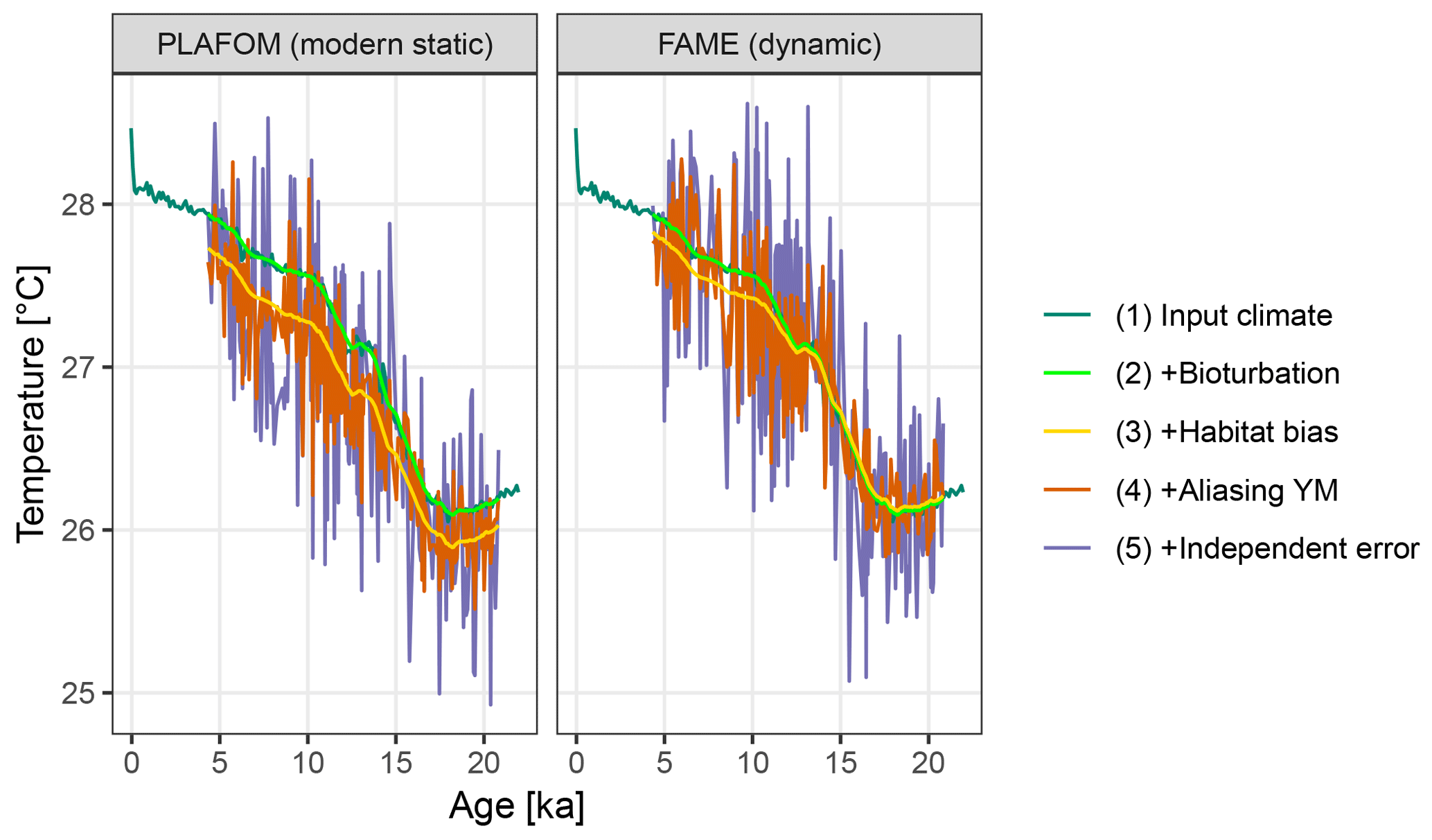
Figure 5 A comparison of forward modelled Mg∕Ca-based pseudo-proxies using static and dynamic seasonal weighting.

4.1.1 Example 1b: dynamic habitat weights

To illustrate the use of dynamic habitat weights we compare here the static weights (derived from PLAFOM with modern climatology) with weights computed using the R implementation of the growth_rate_l09 function from the FAME v1.0 Python module (Roche et al., 2018) included in sedproxy (Fig. 4). For this comparison we run the forward model with an “identity” calibration, i.e. without converting the input climate to proxy units. All other arguments remain the same.

# growth_rate_l09_R requires temp in Kelvin
wts.fame.R <-
  growth_rate_l09_R(
    "ruber", N41.t21k.climate.in + 273.15)

FAME <- ClimToProxyClim(
  clim.signal = N41.t21k.climate.in,
  timepoints = N41.proxy$Published.age,
  calibration.type = "identity",
  habitat.weights = wts.fame.R,
  sed.acc.rate = N41.proxy$Sed.acc.rate.cm.ka,
  sigma.meas = 0.26, sigma.ind = 2,
  n.samples = 30)

Using dynamic habitat weighting from the FAME parameterization results in an apparent mean temperature change between the earliest 2000 years of this record (18–20 ka) and the most recent 2000 years (4–6 ka) of 1.61 ^∘C, compared to 1.72 ^∘C using static weights derived using PLAFOM with modern-day conditions (Fig. 5). In this example, the difference between static and dynamic weights is small but still illustrates the potential for adaptive behaviour of proxy signal carriers to lead to an underestimation of the magnitude of climate shifts. This effect could be larger for a record from a region with a larger seasonal cycle and/or taxon with a more pronounced seasonality in its productivity; also, for comparability with PLAFOM, we used only SST values and not a depth-resolved climate, which would offer further potential for habitat tracking. Note that when creating dynamic weights as a function of temperature, care should also be taken to restrict the occurrence of taxa to their apparent calcification depths.

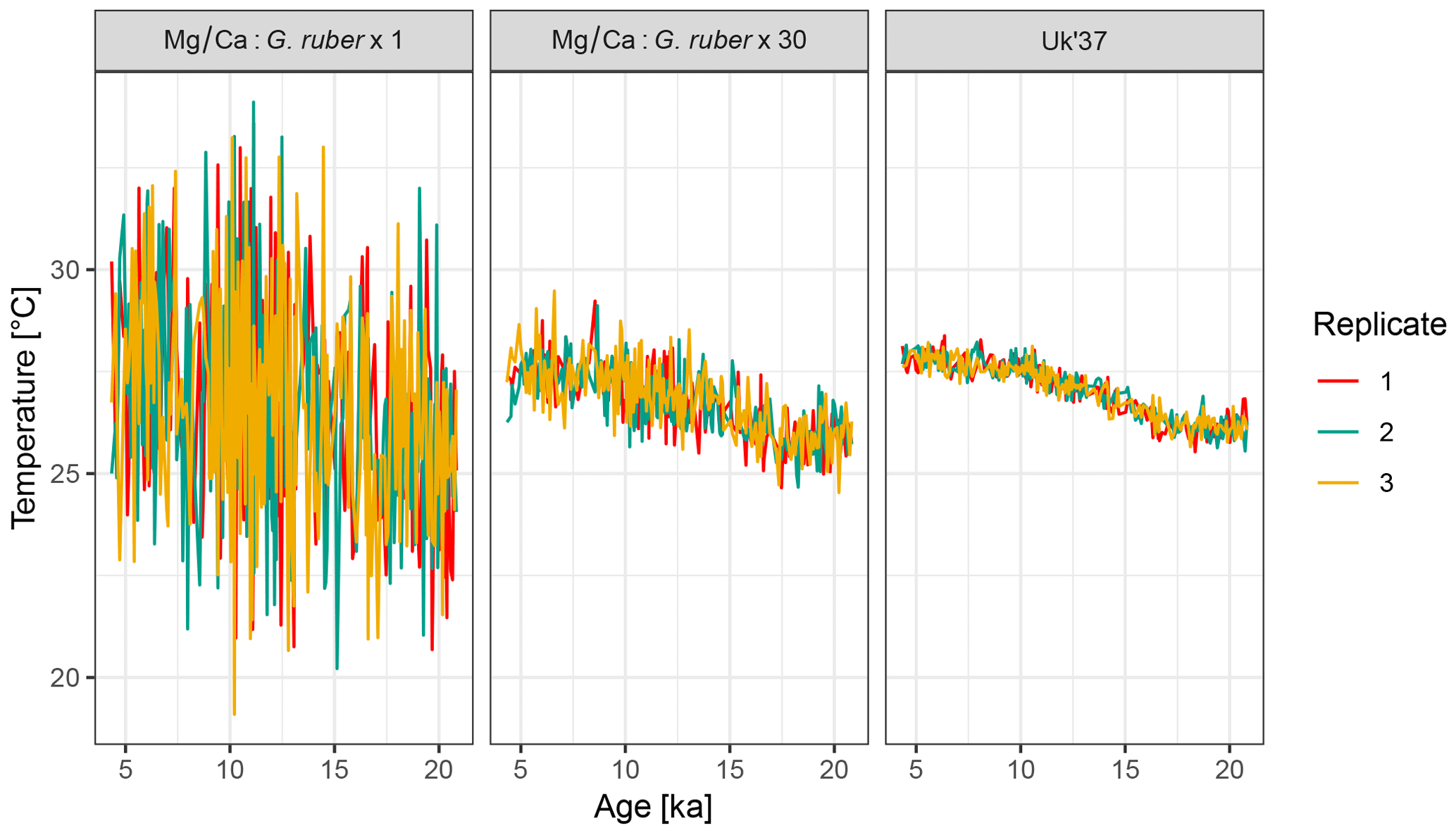
Figure 6 Forward modelled proxy-based temperature reconstructions for Mg∕Ca with 1 and 30 tests of G. ruber, and for U${}_{\mathrm{37}}^{{\mathrm{K}}^{\prime }}$. Three replicate runs of the forward model are shown.

4.2 Example 2: influence of the number of foraminifera per sample

To examine the influence of the number of individual foraminifera per time point on the uncertainty due to seasonal aliasing, we simulate two artificial Mg∕Ca records with 1 and 30 individual foraminifera per sample. For comparison, we also simulate a U${}_{\mathrm{37}}^{{\mathrm{K}}^{\prime }}$ record, for which the sample size per time point is assumed to be infinite. For simplicity we assume that alkenones are uniformly produced throughout the year.

Mg_Ca.1 <- ClimToProxyClim(
  clim.signal = N41.t21k.climate.in,
  timepoints = N41.proxy$Published.age,
  sed.acc.rate = N41.proxy$Sed.acc.rate.cm.ka,
  habitat.weights = N41.G.ruber.seasonality,
  sigma.meas = 0.26, sigma.ind = 2,
  n.samples = 1, n.replicates = 3)

Uk37 <- ClimToProxyClim(
  clim.signal = N41.t21k.climate.in,
  timepoints = N41.proxy$Published.age,
  sed.acc.rate = N41.proxy$Sed.acc.rate.cm.ka,
  sigma.meas = 0.23,
  n.samples = Inf, n.replicates = 3)

The output from three replicate runs with these parameterizations is shown in Fig. 6. For brevity, code to generate the figure and perform the simulation with 30 individuals is not shown here but complete code for all examples is provided in the Supplement.

4.3 Example 3: correlation between two proxy types

Sedproxy can be used to explore the expected correlation between pairs of proxy records. Here we correlate Mg∕Ca- and U${}_{\mathrm{37}}^{{\mathrm{K}}^{\prime }}$-based proxies generated for the same hypothetical sediment core. Records from different locations could be compared by supplying a different input climate matrix for each site.

To emphasize the potential effect of contrasting proxy seasonality on the correlation between two records we use hypothetical seasonal weights. The U${}_{\mathrm{37}}^{{\mathrm{K}}^{\prime }}$ proxy is again assumed to have a constant production with no seasonality, while production of the Mg∕Ca proxy is heavily weighted towards August and September.

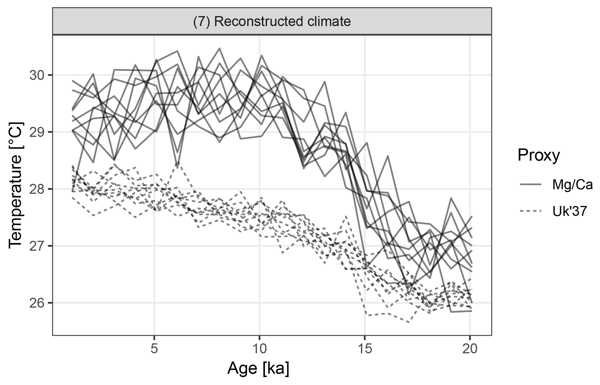
Figure 7 Replicate hypothetical Mg∕Ca- and U${}_{\mathrm{37}}^{{\mathrm{K}}^{\prime }}$-based records. The two proxy types sample different parts of the seasonal cycle. Ten replicate records are shown for each proxy.

We again use the same TraCE-21ka input climate but for simplicity we use a constant sedimentation rate and request proxy values at equally spaced time points. One thousand replicate proxy records are simulated of each type.

# 1000 replicates of a hypothetical Uk'37 and
# Mg/Ca record
Uk37.reps <- ClimToProxyClim(
  clim.signal = N41.t21k.climate.in,
  calibration.type = "Uk37",
  timepoints = seq(100, 21000, by = 1000),
  sed.acc.rate = 25,
  habitat.weights = rep(1/12, 12),
  sigma.meas = 0.23,
  n.samples = Inf,  n.replicates = 1000)

MgCa.reps <- ClimToProxyClim(
  clim.signal = N41.t21k.climate.in,
  calibration.type = "MgCa",
  timepoints = seq(100, 21000, by = 1000),
  sed.acc.rate = 25,
  habitat.weights = c(0,0,0,0,0,0,0.2,0.7,1,0.6,
                      0,0),
  sigma.meas = 0.26, sigma.ind = 2,
  n.samples = 30, n.replicates = 1000)

proxies <- bind_rows(
  "Mg/Ca"=MgCa.reps$everything,
  "Uk'37"=Uk37.reps$everything,
  .id = "Proxy")

proxies <- filter(
  proxies, stage %in% c("reconstructed.climate"))

The Mg∕Ca-based artificial records show greater variance than U${}_{\mathrm{37}}^{{\mathrm{K}}^{\prime }}$ due to a combination of aliasing caused by the finite number of foraminiferal tests and an assumption of higher measurement error (Fig. 7). In addition to a mean offset between the two proxy types, the hypothetical Mg∕Ca proxy shows a much stronger glacial–interglacial transition because the effect of the bias towards recording summer climate increases when the amplitude of the seasonal cycle is larger and this was maximal at around 10 ka.

Figure 8 Correlation between replicate pairs of forward modelled proxy records.

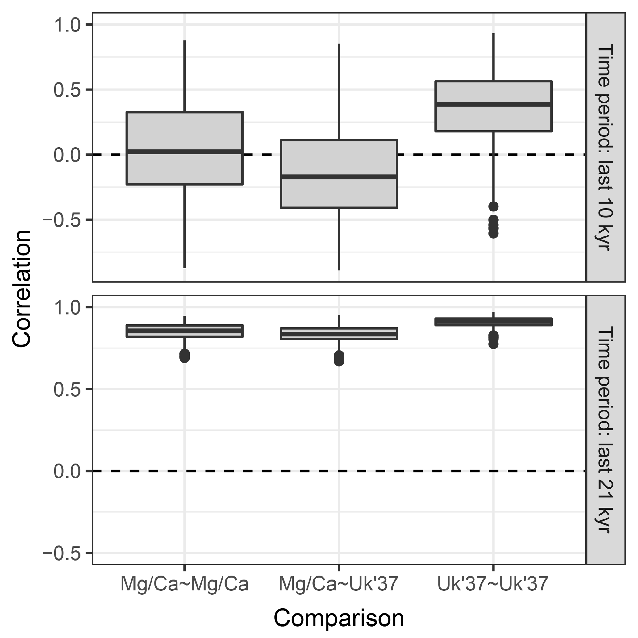
Figure 8 shows the distribution of correlations between replicated pairs of hypothetical Mg∕Ca, U${}_{\mathrm{37}}^{{\mathrm{K}}^{\prime }}$, and Mg∕Ca-U${}_{\mathrm{37}}^{{\mathrm{K}}^{\prime }}$ records, calculated over both the past 10 kry years (Holocene), and the past 21 kry years which include the de-glaciation. Over the Holocene, the average correlation between simulated pairs of proxy records is low, even for pairs of the same proxy type. The average correlation between Mg∕Ca and U${}_{\mathrm{37}}^{{\mathrm{K}}^{\prime }}$ proxy records is even negative, due to the simulated warming annual mean temperature, sampled by the U${}_{\mathrm{37}}^{{\mathrm{K}}^{\prime }}$ record, but slightly cooling summer temperature sampled here by the hypothetical summer growing foraminifera. Similar contrasting trends have been observed between real Mg∕Ca and U${}_{\mathrm{37}}^{{\mathrm{K}}^{\prime }}$ records over the Holocene (Leduc et al., 2010). Correlations between U${}_{\mathrm{37}}^{{\mathrm{K}}^{\prime }}$ pairs are slightly higher than those between Mg∕Ca pairs, due to the lower measurement noise and lack of aliasing we assume for U${}_{\mathrm{37}}^{{\mathrm{K}}^{\prime }}$. When the proxy records include a large climate transition, such as the deglaciation between 21 and 10 ka, correlations between all pairs become high.

4.4 Example 4: individual foraminiferal analysis

In individual foraminiferal analysis (IFA), the population statistics (e.g. standard deviation or range) of proxy values measured on individual foraminifera recovered from the same depth are used to infer changes in climate variability – such as changes in the El Niño Southern Oscillation (ENSO) system (Killingley et al., 1981; Koutavas and Joanides, 2012), or changes in the amplitude of the seasonal cycle (Ganssen et al., 2011; Wit et al., 2010). Sedproxy can be used to simulate IFA by setting n.samples = 1 and n.replicates to the number of individuals measured per time point. This approach bears some similarity with INFAUNAL (Thirumalai et al., 2013); however, while INFAUNAL was designed to test the sensitivity of IFA to the seasonal cycle and inter-annual variability, and therefore includes a specific analysis on the simulated IFA distributions, sedproxy is more general and also includes the effects of bioturbation and habitat weighting.

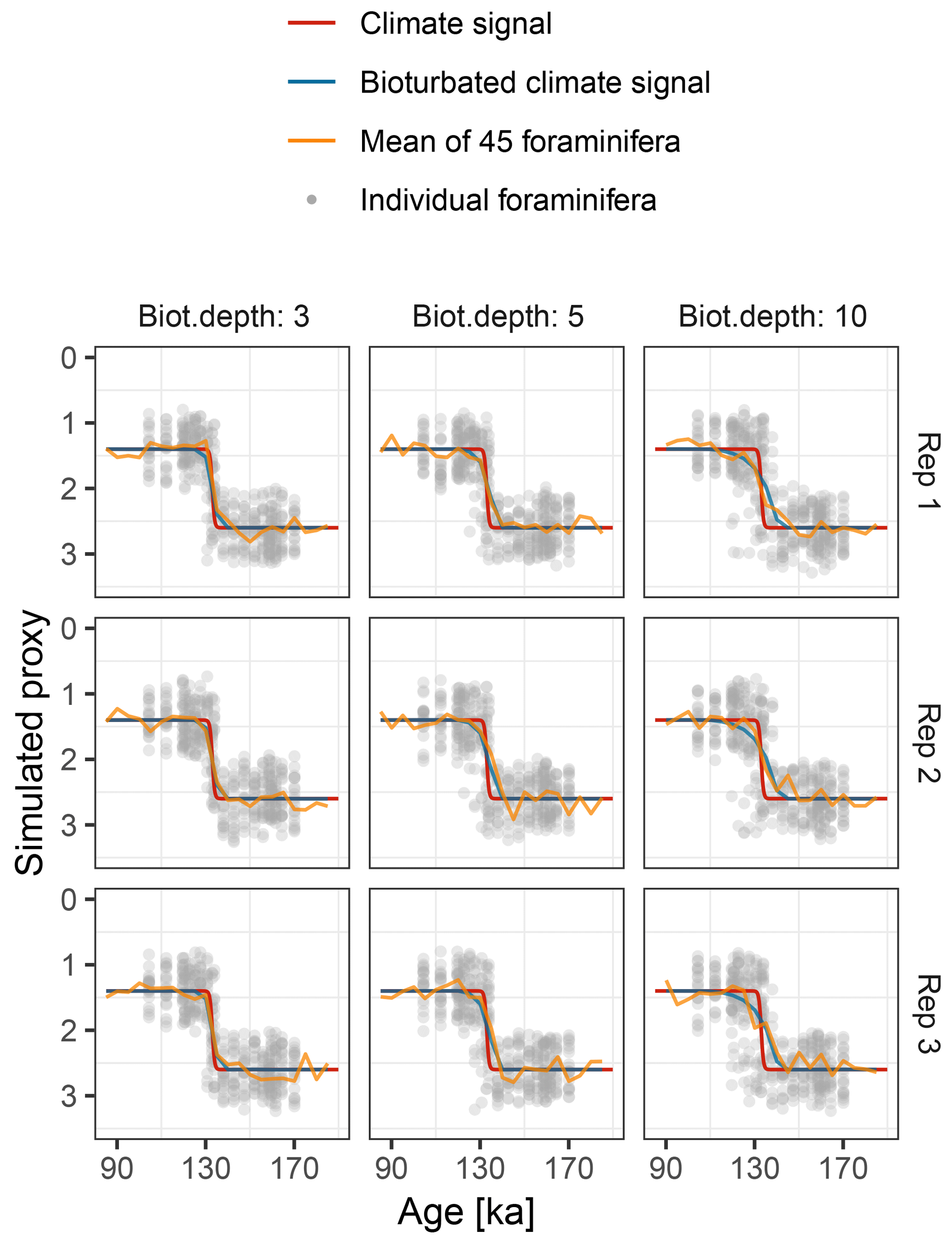
Figure 9 Simulated δ¹⁸O measured from single foraminiferal tests (circles) and bulk samples (lines). Subplots show six replications with the same parameterization.

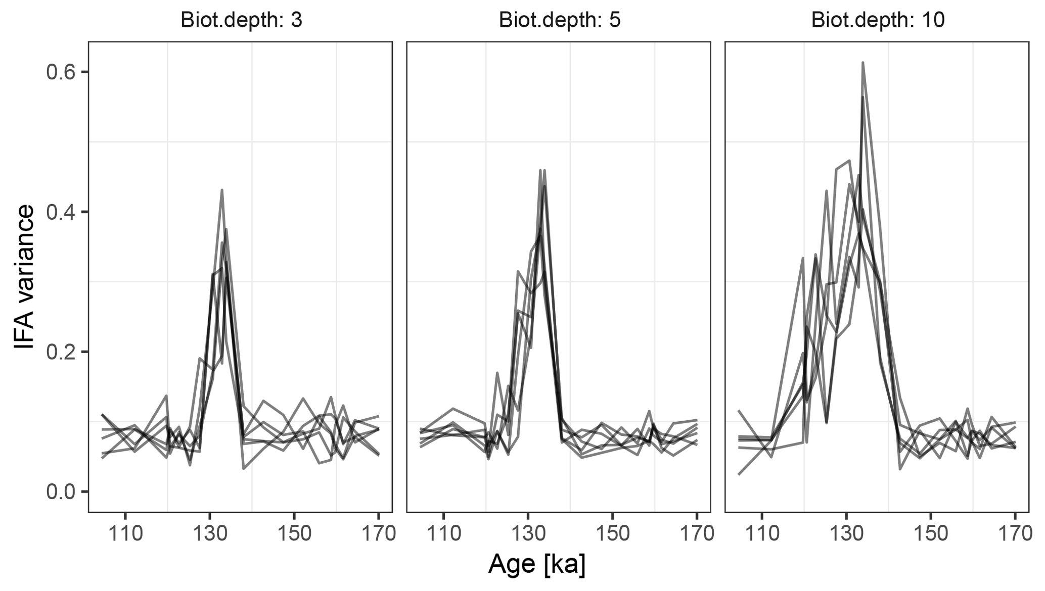
Figure 10 Variance in simulated δ¹⁸O measured on sets of 20 individual foraminiferal tests. Lines show six replications with the same parameterization.

Motivated by the study from Scussolini et al. (2013), which examined changes in the IFA distribution of δ¹⁸O during the penultimate deglaciation, we simulate a case study that demonstrates the effect of bioturbation on the IFA distribution.

To mimic the reconstructed climate signal of Scussolini et al. (2013) we generate an input climate signal in units of δ¹⁸O. We assume a logistic S-shaped climate transition from 1.4 ‰ at 131 ka, to 2.6 ‰ at 135 ka. To this signal we add stochastic climate variability following power law scaling with slope equals 1 (Laepple and Huybers, 2014) and variance equals 0.0025. In this region, the foraminifera Globorotalia truncatulinoides (sinistral coiling variety) calcifies at a mean depth of approximately 520 m, with a standard deviation of 50 m (Scussolini and Peeters, 2013). We model individual variation arising from this using an input climate matrix with 13 columns representing depths from 370 to 670 m, with δ¹⁸O anomalies corresponding to the observed δ¹⁸O gradient of approximately 0.003 ‰ m⁻¹ and habitat weights from a Gaussian distribution with mean equals 520 and SD equals 50. The sedimentation rate is set to 1.3 cm kyr⁻¹. We run the forward model with bioturbation depths of 3, 5, and 10 cm and simulate 20 foraminiferal tests for the IFA analysis, 45 foraminiferal tests for the bulk measurements. We set measurement noise (sigma.meas) to 0.1 ‰ δ¹⁸O for the IFA and the bulk measurements and add no additional individual variation (sigma.ind = 0). These choices reproduce similar IFA and bulk variance as those shown in Scussolini et al. (2013) (Fig. 9). As in Scussolini et al. (2013), for each simulated IFA sample we calculate the variance between individual foraminiferal δ¹⁸O and subtract the variance due to measurement error.

At the observed sediment accumulation rate of 1.3 cm kyr⁻¹ and with assumed bioturbation depths of 3, 5 or 10 cm, the expected standard deviation in ages of material found at a given depth is approximately 2300, 3800, and 7700 years, respectively. Thus, bioturbation mixes material across the deglaciation so that samples with a mean age of between 110 and 140 ka contain a mixture of glacial and inter-glacial material, and hence show a higher standard deviation in δ¹⁸O, with a peak at around 135 ka (Fig. 10). The peak in variance remains clear for bioturbation depths as low as 3 cm, but its absolute value and width are a little lower than that seen in Fig. 2 of Scussolini et al. (2013). At the same time, at bioturbation depths of 3 and 5 cm, the apparent speed of the climate transition is consistent with the sharpness of transition (approximately 8 ka) seen in the bulk record for G. truncatulinoides, but for 10 cm of bioturbation the transition is too spread out. The forward modelling exercise therefore indicates that bioturbation is a possible alternative mechanism for the variance peak, but also indicates that the conclusions are sensitive to the parameterization.

Forward modelling cannot disprove enhanced Agulhas leakage as the source of increased IFA variance across the MIS 5–6 transition (Marine Isotope Stage), and there is other evidence for increased leakage such as the tight coupling between the Agulhas rings proxy and the δ¹⁸O of G. truncatulinoides Scussolini et al. (2015). However, given that bioturbation depths as low as 3 cm still produce a quite visible variance peak, we argue that bioturbation is at least a plausible mechanism behind some of the change in variance over the MIS 5–6 transition.

5 Discussion and conclusions

We present the first forward model for the simulation of sediment-based proxy records from climate data. We include the main well-constrained processes affecting sedimentary signals while keeping it general enough to be usable for a large set of problems in paleo-oceanography. The sedproxy model is implemented as a user-friendly R package in an open-source framework (R Core Team, 2017).

Our forward model relies on and extends the work of many previously published studies and models concerning single processes in the formation of sedimentary records. For example, several prior studies have suggested or investigated the effect of seasonality and/or depth habitat on the recorded proxy signal (Leduc et al., 2010; Liu et al., 2014; Lohmann et al., 2013; Schneider et al., 2010). Others have examined how bioturbation reduces the amplitude of recorded signals and, in combination with noise, puts a limit on the temporal resolution of climate events that can be resolved in proxy records (Anderson, 2001; Goreau, 1980). Further studies have investigated the effect on the resulting record of sampling a small number of foraminiferal tests (Schiffelbein and Hills, 1984; Thirumalai et al., 2013). By integrating these key features of proxy formation into a single model, sedproxy allows for the interactions and combined effect of these processes on the proxy record to be studied for the first time. The relative importance of bioturbation, seasonal biases, aliasing, and other noise sources will vary according to the physical characteristics of the sediment core (e.g. sediment accumulation rate), the length of the record, the amplitude of the seasonal cycle, and the amplitude of the signal that is being reconstructed (e.g. a glacial–interglacial transition vs. ENSO). Most importantly, the type of information that is sought from the proxy record will determine whether these errors are important.

sedproxy has many potential applications in paleoclimate research, not limited to those in the examples given above. It can serve as a forward model to create more realistic surrogate records that can be used to test climate field reconstruction methods (Smerdon et al., 2011) and it can further act as a forward model for inversion-based climate reconstruction methods, i.e. using Bayesian hierarchical models (Tingley and Huybers, 2009) or data assimilation schemes (Klein and Goosse, 2017). Importantly, it allows quantification of the full uncertainty in proxy records related to the processes included in the model. By providing an ensemble of surrogate (pseudo-) proxy realizations, rather than single error values, the full temporal structure of the uncertainty can be characterized. Proxy uncertainty can be determined as a function of timescale, thus separating uncertainties affecting long-term means or time slices, such as the seasonal recording effects, from temporarily independent noise, such as that caused by aliasing of the seasonal cycle. This enables more quantitative comparisons to be made between climate models and proxy data than a classical direct comparison would.

The ability to analyse intermediate stages of the simulated proxy (see Example 1) allows for the effects of different error sources to be evaluated. Used in this way, sedproxy can help optimize and test sampling strategies for sediment cores by evaluating the effect of, for example, the sample thickness, number of foraminifera, or analytical uncertainty in the final record. This information can be used to improve the design of studies and to test, prior to a study, whether signals of interest such as centennial-scale climate variations could theoretically be resolved by the proxy record.

While sedproxy largely relies on well-understood processes that have been previously described in the literature, there is a strong need to refine this and other proxy system models and to confront them with observational data. For this purpose, more systematic multi-proxy studies comparing independent proxies from the same archives (Cisneros et al., 2016; Ho and Laepple, 2016; Laepple and Huybers, 2013; Weldeab et al., 2007) would be useful. Studies analysing replicability inside and between sediment cores in analogue to studies for ice- and coral-based proxies (DeLong et al., 2013; Münch et al., 2016; Smith et al., 2006) would allow for a better constraint of the sample error parameter. Likewise, further investigation of potentially important processes occurring during the preservation of archived proxy signals (Kim et al., 2009; Münch et al., 2017; Zonneveld et al., 2007) would allow these to be included in proxy system models. Finally, modern core-top studies of individual foraminifera distributions (Haarmann et al., 2011) would allow further testing of the assumption that there is a direct link between proxy variability and climate variability.

We hope that this tool will be useful to the paleoclimate research community and we hope that it can provide a starting point for a more complete future proxy system model for sediment proxies. We invite external contributions via the GitHub repository https://github.com/EarthSystemDiagnostics/sedproxy (last access: 23 November 2018).