Connecting the Greenland ice-core and U∕Th timescales via cosmogenic radionuclides: testing the synchroneity of Dansgaard–Oeschger events

During the last glacial period Northern Hemisphere climate was characterized by extreme and abrupt climate changes, so-called Dansgaard–Oeschger (DO) events. Most clearly observed as temperature changes in Greenland ice-core records, their climatic imprint was geographically widespread. However, the temporal relation between DO events in Greenland and other regions is uncertain due to the chronological uncertainties of each archive, limiting our ability to test hypotheses of synchronous change. In contrast, the assumption of direct synchrony of climate changes forms the basis of many timescales. Here, we use cosmogenic radionuclides (¹⁰Be, ³⁶Cl, ¹⁴C) to link Greenland ice-core records to U∕Th-dated speleothems, quantify offsets between the two timescales, and improve their absolute dating back to 45 000 years ago. This approach allows us to test the assumption that DO events occurred synchronously between Greenland ice-core and tropical speleothem records with unprecedented precision. We find that the onset of DO events occurs within synchronization uncertainties in all investigated records. Importantly, we demonstrate that local discrepancies remain in the temporal development of rapid climate change for specific events and speleothems. These may either be related to the location of proxy records relative to the shifting atmospheric fronts or to underestimated U∕Th dating uncertainties. Our study thus highlights the potential for misleading interpretations of the Earth system when applying the common practice of climate wiggle matching.

1 Introduction

Precise and accurate chronologies are critical for understanding past environmental and climatic changes. Global natural and anthropogenic archives can only be directly compared through the development of robust chronological frameworks, enabling studies of the spatiotemporal dynamics of past change. These findings are crucial for understanding the nature and cause of rapid climate changes in the past and hence characterizing the dynamics and feedbacks of past and projected future climate change (Thomas, 2016). However, the applicability, precision, and accuracy of the available dating methods pose strong constraints on our ability to infer leads and lags between climate records and, ultimately, mechanisms of change in the Earth system. Instead, the situation is often reversed: climate changes such as Dansgaard–Oeschger, or DO, events (Dansgaard et al., 1969, 1993) are typically assumed to occur synchronously across the Northern Hemisphere in different climate proxies from various regions and then used as chronological tie points. This so-called “climate wiggle matching” forms the chronological basis of a large part of paleoclimate records (e.g., Bard et al., 2013; Hughen et al., 2006; Henry et al., 2016; Turney et al., 2015), especially in the marine realm where other dating methods suffer from low precision and poorly constrained biases such as the marine radiocarbon reservoir age (Lougheed et al., 2013). Furthermore, it also plays a central role for one of the most widely used dating methods in paleosciences – the radiocarbon dating method. The current radiocarbon dating calibration curve (IntCal13, Reimer et al., 2013) is constructed from accurately dated tree-ring chronologies back to 13.9 ka BP (ka BP is kilo-years before present, which is 1950 CE). Beyond this time, which encompasses all DO events, about one-fourth of the data underlying IntCal13 obtain their absolute age from climate wiggle matching.

Climate wiggle matching has the obvious drawback that the leads and lags between different climate records cannot be studied once the records have been forced to align. The approach critically rests on the assumptions that (i) the climate change indeed occurred synchronously everywhere and that (ii) the (sometimes fundamentally different) proxies in question record the changes in a similar way and without intrinsic delays. These assumptions, however, can very rarely be rigorously tested, but when they are, ample evidence is revealed that questions their universal validity. Lane et al. (2013) showed that rapid climate change in the North Atlantic region may be time transgressive with regional leads and lags of the order of a century. Nakagawa et al. (2003) argued that the onset of Greenland Interstadial 1e (GI-1e; Rasmussen et al., 2014a) occurred multiple centuries after the associated climate shift in Japan, and subsequent revisions of the underlying timescales (Staff et al., 2013; Bronk Ramsey et al., 2012; Seierstad et al., 2014) did not resolve this conundrum. Buizert et al. (2015) inferred that the Southern Ocean response to DO events is delayed by about 200 years on average, while the atmosphere around Antarctica reacted instantaneously (Markle et al., 2016). Baumgartner et al. (2014) found asynchronies between ice-core proxies for local Greenland temperature (δ¹⁵N) and the tropical and midlatitude hydrological cycle (CH₄) during some DO events. They discussed the possibility that the climate changes in polar and low-latitude regions may indeed be synchronous, but that atmospheric CH₄ concentrations rise with a delay during some DO events because of compensating changes in the source strengths of the Northern and Southern Hemisphere wetlands. Alternatively, their findings can be explained via a real delay between Greenland climate change and the activation of CH₄ source areas during certain DO events. Fleitmann et al. (2009) reported timing differences of DO events in Greenland ice cores and speleothems, albeit largely within dating uncertainties. However, they also found significant differences between speleothem records outside their chronological uncertainties. This is complemented by a recent study showing that the duration of a stadial–interstadial transition can differ by up to 300 years between different East Asian speleothems (Li et al., 2017), emphasizing the question of whether we should expect the onset, midpoint, or end point of DO events to occur simultaneously, as this choice will lead to different results when aligning the records.

In this paper, we attempt to provide improved constraints on the paradigm of climate synchroneity. We employ cosmogenic radionuclides as a climate-independent synchronization tool between the Greenland ice-core timescale (Andersen et al., 2006; Rasmussen et al., 2006; Seierstad et al., 2014; Svensson et al., 2006, 2008; Vinther et al., 2006) and the U∕Th timescale (Broecker, 1963; Edwards et al., 1987; Cheng et al., 2013a) and strongly reduce the absolute dating error of the Greenland ice cores back to 45 000 years BP. This allows us to compare the timing of DO-type variability seen in key paleoclimate records with unprecedented precision: the Greenland ice cores and U∕Th-dated (sub)tropical speleothems.

2 Cosmogenic radionuclides as synchronization tools

Cosmogenic radionuclides (such as ¹⁴C, ¹⁰Be, and ³⁶Cl) are produced in a nuclear cascade that is triggered when galactic cosmic rays (GCRs) collide with the Earth atmosphere's constituents (Lal and Peters, 1967). While the GCR flux outside the heliosphere can be assumed to be constant over the past million years (Vogt et al., 1990), the flux arriving at Earth is modulated by the strength of the helio-magnetic and geomagnetic fields (Masarik and Beer, 1999). This causes the production rates of cosmogenic radionuclides to be inversely related to changes in solar activity and/or the strength of the geomagnetic field. This modulation effect leaves a globally synchronous, externally forced signal in cosmogenic radionuclide records around the world. Hence, they can serve as a powerful synchronization tool for climate archives from different regions. The challenge lies in estimating potential non-production-related impacts on radionuclide concentrations in a given archive that may result from geochemical and meteorological processes.

After production, ¹⁴C is oxidized to ¹⁴CO₂ and enters the carbon cycle. Changing ¹⁴C production rates thus alter the atmospheric ¹⁴C∕¹²C ratio (expressed as per mille Δ¹⁴C, which is ¹⁴C∕¹²C corrected for fractionation and decay relative to a standard, denoted Δ in Stuiver and Polach, 1977). Due to carbon cycle effects, these variations in Δ¹⁴C are dampened and delayed with respect to the causal production rate changes (Siegenthaler et al., 1980; Roth and Joos, 2013). In addition to variable production rates, changes in the exchange rates between the different carbon pools can alter Δ¹⁴C. The world's oceans in particular have a significantly lower Δ¹⁴C than the contemporary atmosphere due to their long carbon residence time (Craig, 1957). Thus, variations in the ¹⁴C exchange rates between the ocean and the atmosphere will alter atmospheric Δ¹⁴C independent of production rate changes.

¹⁰Be attaches to aerosols and is transported from the stratosphere to the troposphere within 1–2 years (Raisbeck et al., 1981), mainly via midlatitude tropopause breaks (Heikkilä et al., 2011). It has no active geochemical cycle, so its atmospheric concentration is a more direct recorder of production rate changes compared with Δ¹⁴C. However, ¹⁰Be transport and deposition in the troposphere are guided by local meteorology and thus susceptible to changes thereof (Heikkilä and Smith, 2013; Pedro et al., 2011). This can cause variations in ¹⁰Be records that are not related to production rate changes. Furthermore, a so-called “polar bias” (i.e., an overrepresentation of polar as opposed to global production rate changes) has been proposed for ice-core records (Bard et al., 1997). This would lead to subdued geomagnetic and enhanced solar modulation of ice-core radionuclide records due to the geometry of the geomagnetic field. However, there is no consensus in different empirical studies and modeling experiments on whether this effect is present and the results may also vary regionally (Bard et al., 1997; Heikkilä et al., 2009a; Pedro et al., 2012; Adolphi and Muscheler, 2016; Muscheler and Heikkilä, 2011; Field et al., 2006).

The transport and deposition of ³⁶Cl in its aerosol phase are comparable to ¹⁰Be. However, in addition to an aerosol phase, ³⁶Cl also has a gaseous phase (H³⁶Cl), which is likely dominant in the stratosphere (Zerle et al., 1997). In the troposphere, the partitioning between the aerosol and gas phase is not well understood. It may vary in space and time (Lukasczyk, 1994) and can change rapidly depending on pH (Watson et al., 1990). The gaseous H³⁶Cl phase can also be lost from acidic ice in low accumulation sites after deposition, which is less relevant for the high accumulation sites studied here (Delmas et al., 2004). In Greenland, similar to ¹⁰Be, the dominant deposition process of ³⁶Cl is wet deposition (Heikkilä et al., 2009b), which is supported by the overall similarity of ³⁶Cl and ¹⁰Be variations recorded in ice cores (Wagner et al., 2001b; Muscheler et al., 2005).

As a result, all three radionuclides depend on the same production mechanism, which causes their production rates to covary globally. This signal can be exploited for global synchronization of paleorecords from natural archives. However, to identify these common changes, their different geochemistry needs to be accounted for. In the case of radiocarbon this is achieved through carbon cycle modeling to deconvolve the effects of the carbon cycle on the relation between ¹⁴C production rates and Δ¹⁴C (Muscheler et al., 2004). For ¹⁰Be and ³⁶Cl, fluxes can be calculated from ice accumulation rates. This provides a first-order correction for changing paleoprecipitation rates on the ice sheet and their influence on the radionuclide concentrations. In reality, aerosol transport to the ice sheet is more complex and depends on changes in transport velocity, pathways, and scavenging effects en route (Schüpbach et al., 2018), which are difficult to constrain for ¹⁰Be due to its stratospheric origin. Instead, comparisons of fluxes and concentrations to other climate proxies can inform us about potential climate influences on ¹⁰Be and³⁶Cl transport and deposition (Adolphi and Muscheler, 2016). It is currently not possible to quantitatively correct either of the radionuclides for these non-production influences since neither past carbon cycle changes nor atmospheric circulation changes are sufficiently well known. However, the potential amplitude of non-production rate changes can be assessed through sensitivity experiments and added as an uncertainty for the production rate signal (Adolphi and Muscheler, 2016; Köhler et al., 2006).

The potential of this synchronization tool has been demonstrated multiple times to infer differences between the tree-ring and ice-core timescales (Adolphi and Muscheler, 2016; Muscheler et al., 2014a; Southon, 2002), test the accuracy of the radiocarbon calibration curve (Adolphi et al., 2017; Muscheler et al., 2008, 2014b), and synchronize ice cores from both hemispheres (Raisbeck et al., 2007, 2017).

3 Methods and data

3.1 Ice-core data

The ice-core ¹⁰Be and ³⁶Cl data used in this study are shown in Fig. 1. We focus on records that have been robustly linked to the GICC05 timescale (Andersen et al., 2006; Rasmussen et al., 2006, 2008; Seierstad et al., 2014; Svensson et al., 2008). Hence, the majority of the data stems from the deep Greenland ice cores GRIP, GISP2, and NGRIP. In addition, we use Antarctic ¹⁰Be fluxes from EDC, EDML, and Vostok that have been anchored to GICC05 by matching the solar variability present in all ¹⁰Be records and volcanic tie points (Raisbeck et al., 2017).

Figure 1 Data used in this study. (a–g) Individual ice-core records of GRIP ¹⁰Be (Baumgartner et al., 1997b; Muscheler et al., 2004; Wagner et al., 2001a; Yiou et al., 1997; Adolphi et al., 2014), GRIP ³⁶Cl (Baumgartner et al., 1997a, 1998; Wagner et al., 2001b; Wagner et al., 2000), GISP2 ¹⁰Be (Finkel and Nishiizumi, 1997), and ¹⁰Be from EDC, EDML, Vostok, and NGRIP (all Raisbeck et al., 2017). Each record represents deposition fluxes (green) and “climate-corrected” fluxes (purple; see text). In addition, each panel contains the stack of all ice-core records (black; see text). (h) ¹⁰Be production rates modeled from two geomagnetic field intensity reconstructions: GLOPIS (green; Laj et al., 2004) and based on Black Sea sediments (purple; Nowaczyk et al., 2013) using the production rate model by Herbst et al. (2016). The ice-core radionuclide stack is shown in black. All records in (a–h) are shown on the GICC05 timescale (Seierstad et al., 2014) and normalized to (i.e., divided by) their mean. (i) Absolutely dated ¹⁴C data from Lake Suigetsu (yellow; Bronk Ramsey et al., 2012), Hulu Cave (blue; Southon et al., 2012), Bahamas speleothems (purple; Hoffmann et al., 2010), and various tropical coral datasets (Bard et al., 1998; Cutler et al., 2004; Durand et al., 2013; Fairbanks et al., 2005; shown in light blue, olive, red, and green, respectively). The black lines encompass the ±1σ uncertainties of IntCal13 (Reimer et al., 2013).

By calculating fluxes we make a first-order correction for the changing snow accumulation rates between stadials and interstadials and their influence on radionuclide concentrations (Wagner et al., 2001b; Johnsen et al., 1995; Rasmussen et al., 2013; Finkel and Nishiizumi, 1997). The accumulation rates for each ice core are based on their annual layer thickness – derived from their individual timescales – corrected for ice thinning. For the Greenland ice cores this thinning function is based on a 1-D ice flow model (Dansgaard and Johnsen, 1969; Johnsen et al., 2001, 1995; Seierstad et al., 2014). For the Antarctic ice cores we use the strain rate derived from the Bayesian ice-core dating effort AICC12 (Veres et al., 2013). These strain rates are inherently uncertain, and independently derived accumulation rate estimates differ by up to 10 %–20 % in the glacial (Gkinis et al., 2014; Rasmussen et al., 2013; Guillevic et al., 2013). However, these differences are largely systematic and change only on multi-millennial timescales. The shorter-term changes in accumulation rates are a more direct function of the timescale that determines the age–depth relationship, and thus annual layer thickness, and is very precise for increments of the core (Rasmussen et al., 2006). This is important to note, as we mainly exploit production rate changes on centennial-to-millennial timescales for synchronization.

To test for additional climate influences on ¹⁰Be or ³⁶Cl deposition in the ice cores, we followed the approach by Adolphi and Muscheler (2016). For each ice core we calculated multiple linear regression models using δ¹⁸O and snow accumulation rates as predictors for ¹⁰Be (³⁶Cl) fluxes and subtracted the obtained model from the ¹⁰Be (³⁶Cl) data. We denote the resulting record as the “climate-corrected flux” (Flux_c). This approach may correct climate effects on ¹⁰Be (³⁶Cl) deposition insufficiently, or it may overcorrect them, so it cannot be assumed per se that the resulting record is more reliable than the original fluxes. Nevertheless, it provides a first-order sensitivity test for the ice-core records with respect to climate-related transport and depositional effects on ¹⁰Be (³⁶Cl) fluxes.

To combine all ice-core records, we calculated their mean (denoted as “stack”, Fig. 1) using Monte Carlo bootstrapping (Efron, 1979). Using seven ice-core records in two versions (flux and flux_c) yields a total number of 14 samples. In each iteration, 14 samples are randomly drawn (with replacement; i.e., each record can be drawn multiple times), perturbed within measurement errors, and stacked. By repeating this procedure 1000 times we obtain an average relative standard deviation of 8 % between the derived stacks, which is comparable to the measurement uncertainty of individual measurements but larger than the expected error of the mean; this points to systematic differences between the records. For the period over which we have data from both hemispheres this standard deviation is only slightly higher (10 %). Even though this is only a relatively short period (see Fig. 1), it contains multiple DO events that are expressed differently in Northern and Southern Hemisphere climate. Thus, this agreement can serve as an indication that climate effects do not dominate the signal.

3.2 Radiocarbon data

For the purpose of this study we have to focus on radiocarbon records that are absolutely dated. Furthermore, the length and sampling resolution of the records need to be sufficient to resolve centennial-to-millennial production rate changes. The records that fulfill these criteria are shown in Fig. 1 and comprise ¹⁴C data from various U∕Th-dated coral records (Bard et al., 1998; Durand et al., 2013; Cutler et al., 2004; Fairbanks et al., 2005), as well as ¹⁴C measured in two speleothems (Southon et al., 2012; Hoffmann et al., 2010). In addition, we use the ¹⁴C record from Lake Suigetsu (Bronk Ramsey et al., 2012) since the U∕Th-dated records do not directly reflect atmospheric ¹⁴C, only the ocean mixed layer (corals), and in the case of speleothems a mixture of atmospheric and soil CO₂ and carbonate bedrock from above the cave. The timescale of the Lake Suigetsu record is based on varve counting, corrected for long-term systematic errors by matching its ¹⁴C record to the ¹⁴C variations in speleothems (Bronk Ramsey et al., 2012). Hence, it is not truly independently dated. However, similar to ice-core layer counting, this varve count adds constraints, especially on centennial timescales, so Δ¹⁴C variations on these timescales should be relatively unaffected by this tuning to the speleothem ¹⁴C data. Thus, even though the timescale may not be independent, this record can still be used to verify the existence of Δ¹⁴C variations in the atmosphere seen in the mixed layer records.

In addition, we use the available tree-ring records back to 14 000 cal BP (calibrated before present, 1950 CE) in the revised version by Hogg et al. (2016) (not shown in Fig. 1 for clarity).

3.3 Carbon cycle modeling

To be able to compare ice-core and radiocarbon records directly we have to account for the effects of the carbon cycle. Following earlier studies (Muscheler et al., 2004, 2008), we use a box-diffusion carbon cycle model (Siegenthaler et al., 1980) to model Δ¹⁴C from the ice-core radionuclide records. We assume that ice-core ¹⁰Be (³⁶Cl) variations are proportional to ¹⁴C production rate changes (see also the following section) and model Δ¹⁴C anomalies from each realization of the ice-core stack, as well as the single ice-core records (Fig. 2). It can be seen that the modeled Δ¹⁴C records from the individual ice-core records differ in their long-term trends since the carbon cycle integrates over time so that relatively small but systematic differences in the radionuclide fluxes (possibly arising from uncertainties in the strain rates) have a significant effect on longer timescales. However, all records show the same overall evolution of Δ¹⁴C. Furthermore, especially when subtracting the long-term trend and isolating variations on timescales shorter than 5000 years, the agreement is very high (on average within 15 ‰ at 1σ; Fig. 2b), which is the part of the signal that we will be exploiting in our synchronization effort.

3.3.1 Production rate ratio

Modeling Δ¹⁴C values from ¹⁰Be measurements is based on the assumption that ¹⁰Be and ¹⁴C production rate changes are proportional to each other. However, different production rate models differ in their sensitivity of ¹⁴C and ¹⁰Be production rate changes to variations in the geomagnetic field (Cauquoin et al., 2014). For a given geomagnetic field change, the production rate model by Masarik and Beer (1999, 2009) yields 30 %–50 % lower ¹⁰Be production rate changes than the calculations by Poluianov et al. (2016) and Herbst et al. (2016). For ¹⁴C, on the other hand, all models yield roughly similar amplitudes. This leads to differences in the ¹⁴C∕¹⁰Be production rate ratio for a given change in the geomagnetic field. If Masarik and Beer (1999) are correct, the variations in ice-core ¹⁰Be records have to be upscaled by 30 %–50 % to be proportional to ¹⁴C production rate changes, while no such scaling is necessary when the other production rate models are used. In addition, the amplitudes in ¹⁴C and ¹⁰Be may differ due to the presence of polar bias (see Sect. 2). If this effect was present, then geomagnetic field changes should cause bigger variations in ¹⁴C than ¹⁰Be.

Since the presence of a polar bias is debated and the physical reason for the differences between the production rate models is unresolved, we chose an empirical approach to scale the ice-core record appropriately.

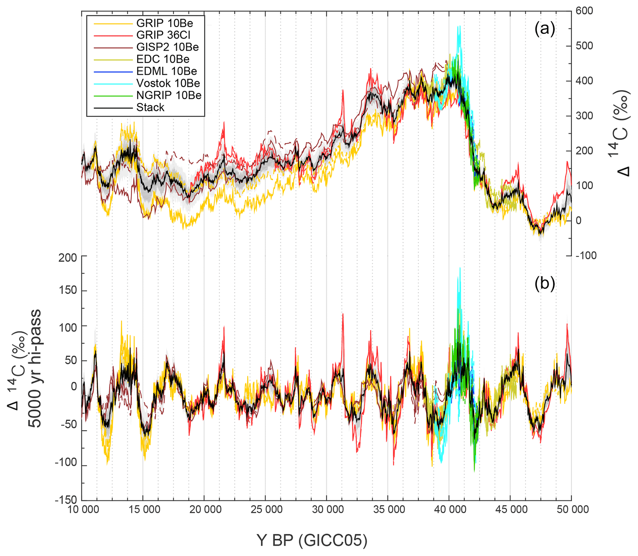
Figure 2 Modeled Δ¹⁴C anomalies from individual ice-core records (see legend; solid lines are based on radionuclide fluxes, while dashed lines are inferred from flux_c) and the realizations of the ice-core stack (black line shows the mean of all realizations, dark and light grey shading encompass 68.2 % and 95.4 % probability ranges). (a) The unfiltered model output. (b) The records after variations with frequencies < 1 ∕ 5000 a⁻¹ have been subtracted (FFT-based filter).

We use three geomagnetic field intensity reconstructions around the Laschamp geomagnetic field minimum (Laj et al., 2000, 2004; Nowaczyk et al., 2013) and calculate the resulting ¹⁰Be production rate changes using the production rate models by Masarik and Beer (1999) and Herbst et al. (2016) (Fig. 3a–c). Subsequently, we scale the ice-core ¹⁰Be record to minimize the root mean square error (RMSE) between ice-core and geomagnetic-field-based records (Fig. 3d). It can be seen that the RMSE reaches a minimum for a ¹⁰Be scaling factor of ∼1 (for Masarik and Beer, 1999) and ∼1.3 (for Herbst et al., 2016). This represents a fortunate coincidence; irrespective of which production rate model is used, the amplitude of the ice-core ¹⁰Be variations has to be increased by approximately 30 % to match ¹⁴C. If the production rate model by Masarik and Beer is used, then the amplitude of the ice-core ¹⁰Be record is in agreement with geomagnetic field data, but due to the higher production sensitivity of ¹⁴C (see above), ¹⁰Be variations have to be increased by ∼30 %. Similarly, if the production rate model by Herbst et al. is used, then the amplitude of the ice-core ¹⁰Be record is 30 % smaller than implied by geomagnetic field data (possibly due to a polar bias), while the sensitivity of ¹⁴C and ¹⁰Be is the same. Again, the net effect is that the ¹⁰Be variations have to be scaled up by 30 % for the comparison to ¹⁴C.

Figure 3 Comparison of ice-core-based and geomagnetic-field-based reconstructions of ¹⁰Be production rates. (a–c) The ice-core stack (black) in comparison to ¹⁰Be production rates based on geomagnetic field reconstructions and two different production rate models (Herbst et al., 2016, in pink and Masarik and Beer, 1999, in green). (a) The Black Sea geomagnetic field record (Nowaczyk et al., 2013), (b) the NAPIS geomagnetic field stack (Laj et al., 2000), and (c) the GLOPIS geomagnetic field stack (Laj et al., 2004). (d) The RMSE between the ice-core data and the geomagnetic-field-based records when variations in the ice-core record are scaled by different factors (x axis). The colors correspond to the production rate models. The line styles indicate the geomagnetic field records (see legend) and the symbols denote the RMSE minima.

3.3.2 The state of the carbon cycle

As mentioned in Sect. 2, a quantification of transient carbon cycle changes and their influence on Δ¹⁴C is challenged by insufficient knowledge of inventories and processes. The contribution of single processes to Δ¹⁴C changes over the last glacial cycle is likely within 30 ‰ and, due to compensating effects, their combination is likely not bigger than 40 ‰ (Köhler et al., 2006). Here we use the Laschamp event to estimate the state of the ocean ventilation around 40 ka BP.

The datasets underlying IntCal13 all show an increase of about 320 ‰ in Δ¹⁴C into the Laschamp event (Fig. 4), albeit at different absolute levels (see Fig. 1). This is ∼ 100 ‰ more than the compiled IntCal13 curve itself implies. This disagreement can be explained by differences in timing and absolute Δ¹⁴C between the different datasets leading to smoothing and dampening of Δ¹⁴C variations during the construction of IntCal13. Also, geomagnetic field changes yield a Δ¹⁴C change more in line with the individual ¹⁴C datasets than with IntCal13, even when assuming a preindustrial carbon cycle.

To estimate the mean state of the carbon cycle during this period, we run our carbon cycle model with different (constant) values of ocean diffusivity. We find that modeled and measured Δ¹⁴C around the Laschamp event match best in amplitude when we run the model under conditions in which ocean ventilation is reduced to ∼75 % of its preindustrial value (Fig. 4). This is in broad agreement with previous modeling experiments (Köhler et al., 2006; Roth and Joos, 2013) and proxy data (Henry et al., 2016).

In the following, we will use this estimate for the parameterization of our model. As mentioned above, a transient adjustment of carbon cycle parameters is uncertain and will hence not be attempted. Instead, we ascribe an associated uncertainty to the modeled Δ¹⁴C based on the carbon cycle sensitivity experiments by Köhler et al. (2006). Furthermore, it should be noted that by only using (filtered) Δ¹⁴C anomalies as synchronization targets, we (i) avoid systematic carbon cycle influences on Δ¹⁴C levels and (ii) minimize transient carbon-cycle-related changes in Δ¹⁴C (Adolphi and Muscheler, 2016).

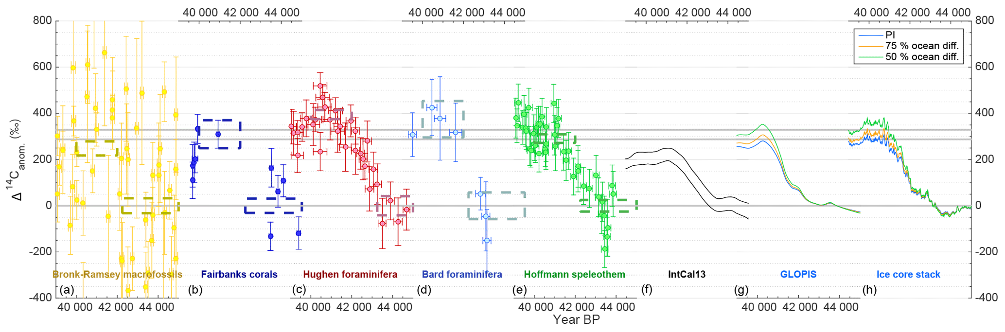
Figure 4 The Laschamp event in measured and modeled Δ¹⁴C. (a–f) Δ¹⁴C anomalies in macrofossils from Lake Suigetsu (yellow; Bronk Ramsey et al., 2012), tropical corals (blue; Fairbanks et al., 2005), foraminifera from Cariaco Basin sediments (red; Hughen et al., 2006), foraminifera from Iberian Margin sediments (light blue; Bard et al., 2013), Bahamas speleothems (green; Hoffmann et al., 2010), and IntCal13 (black; Reimer et al., 2013). All data are shown as anomalies to their error-weighted mean prior to the Laschamp event, i.e., the Δ¹⁴C increase. The dashed boxes encompass the time periods and Δ¹⁴C uncertainties (error of the error-weighted mean) used for the definition of the pre- and post-Laschamp event levels. (g, h) Modeled Δ¹⁴C using the GLOPIS (Laj et al., 2004) geomagnetic field record and the ice-core stack as production rate inputs. The different colored lines reflect different carbon cycle scenarios (see legend; PI denotes preindustrial). The conversion of geomagnetic field intensity to ¹⁴C production rate is based on the production rate model by Herbst et al. (2016). Note that the amplitude of the ¹⁰Be variations has been increased by 30 % as discussed in Sect. 3.3.1.

3.4 Synchronization – effects of the carbon cycle and the archive

The synchronization method follows Adolphi and Muscheler (2016) and is outlined and tested in detail therein. In brief, sections of modeled (ice-core-based) Δ¹⁴C anomalies are compared to the measured Δ¹⁴C. For our analysis we employ high-frequency changes in Δ¹⁴C since carbon cycle changes have only limited effects on atmospheric Δ¹⁴C on shorter timescales (Adolphi and Muscheler, 2016). Similarly, as shown in Fig. 2, the agreement of the different ice-core records is better on shorter timescales. In this study, we employ two types of high-pass filtering: an FFT-based high-pass filter and simple linear detrending. The choice of filter is based on the data sampling resolution. For the highly resolved tree-ring data we use a 1000-year high-pass FFT filter, while the lower-resolved and more unevenly sampled coral, speleothem, and/or macrofossil data are filtered by linear detrending to avoid the interpolation to equidistant resolution required for FFT analysis. Similarly, the high sampling resolution of the tree-ring data allows us to compare the data in 2000-year windows, while we increase the window length to 4000 and 5000 years for the lower-resolved data prior to 14 ka BP. The exact frequencies and window lengths are also given in the Results section. Using the same statistics as for radiocarbon wiggle-match dating (Bronk Ramsey et al., 2001), we then infer a probability density function (PDF) for the timescale difference between the modeled and measured Δ¹⁴C records. For details on the statistics of this methodology we refer the reader to Adolphi and Muscheler (2016). Here we focus instead on additional uncertainties that arise when comparing modeled atmospheric Δ¹⁴C to ¹⁴C records from the ocean mixed layer (corals) or speleothems.

Δ¹⁴C variations in the atmosphere are dampened and delayed compared to the causal production rate changes. Both factors, attenuation and delay, depend on the frequency of the production rate change (Roth and Joos, 2013; Siegenthaler et al., 1980). The dampening is largest at high frequencies and decreases with longer periods. On the other hand, the apparent peak-to-peak delay between sinusoidal production rate changes and the resulting Δ¹⁴C change increases with increasing wavelengths. Similar effects occur when comparing atmospheric and oceanic Δ¹⁴C changes to each other: the ocean reacts to atmospheric Δ¹⁴C changes with a delayed and dampened response that is wavelength dependent. Hence, we need to take these factors into account when comparing a modeled atmospheric Δ¹⁴C record to mixed layer marine records. However, the frequency dependence of the attenuation and delay makes it difficult to explicitly correct for this since atmospheric Δ¹⁴C changes vary on different timescales simultaneously. Furthermore, the coral records vary in their sampling frequency and often it is not precisely known over how much time an individual ¹⁴C sample integrates.

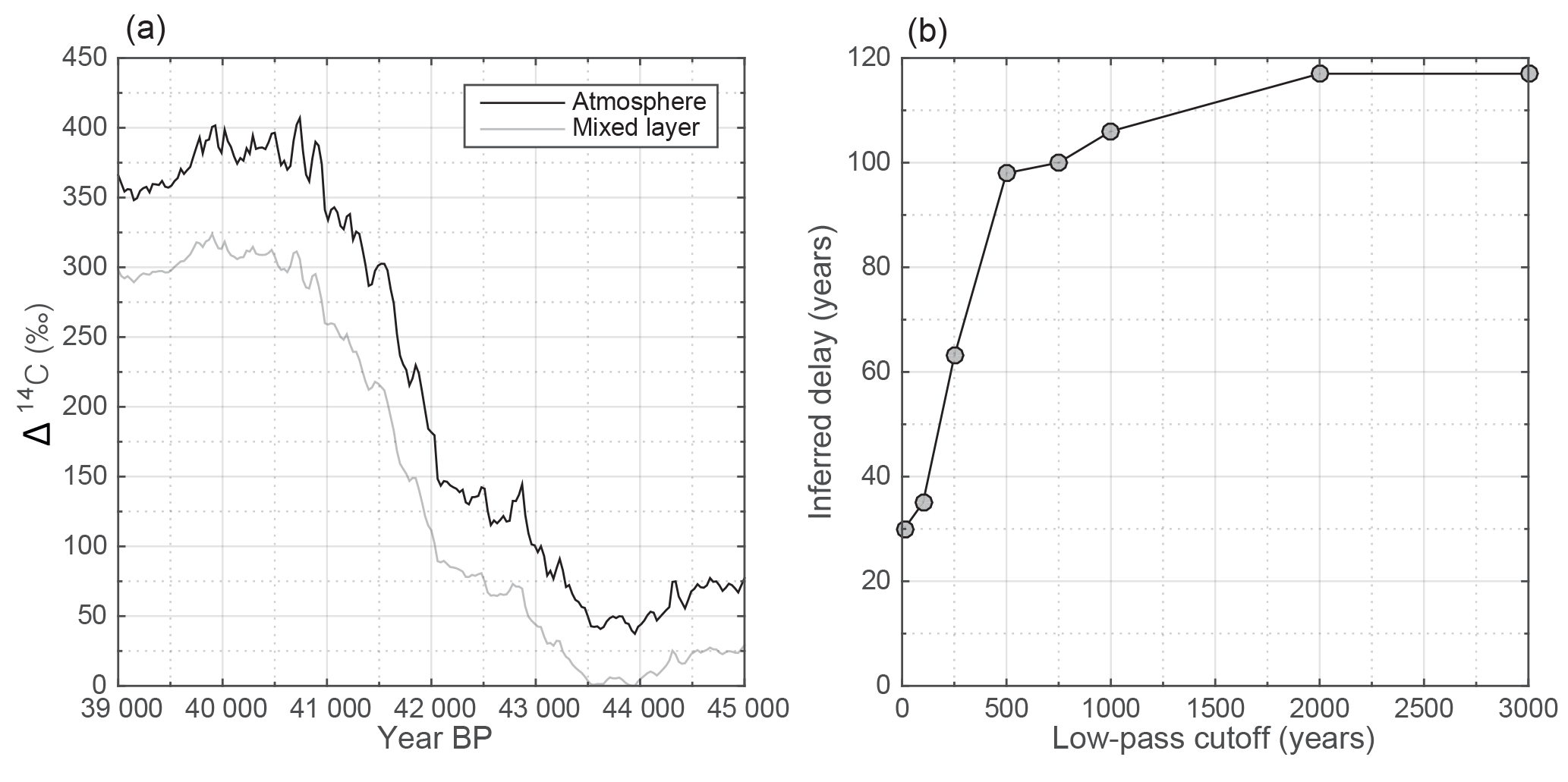
Figure 5 The delay between Δ¹⁴C in the atmosphere and ocean mixed layer. (a) Modeled Δ¹⁴C from the ice-core stack around the Laschamp event. The modeled atmospheric Δ¹⁴C is shown in black, while the ocean mixed layer is shown in grey. (b) The inferred delay from our synchronization method when comparing the atmospheric to the mixed layer signal for different low-pass filters of the mixed layer signal (x axis).

Figure 5 shows a sensitivity test regarding these effects. We modeled Δ¹⁴C from the ice-core stack around the Laschamp event and compared the atmospheric Δ¹⁴C to the mixed layer Δ¹⁴C in the model. To simulate the effect of varying averaging effects of the coral samples, we low-pass filtered the mixed layer signal with increasing cutoff wavelengths. For each filter, we then inferred the apparent delay between the mixed layer (i.e., the “coral”) and the atmosphere. In doing so we infer that even though the signal is dominated by a long-lasting Δ¹⁴C increase, the inferred delay is small (∼30 years) as long as the coral samples do not integrate over long times. Only when assuming that each coral sample averages over more than 1000 years do we infer delays of about 120 years. Nevertheless, this experiment also shows that within reasonable bounds of averaging, the delay of the mixed layer to atmospheric signal is limited.

The speleothem Δ¹⁴C reacts differently than the ocean mixed layer. The so-called dead carbon fraction (DCF) of a speleothem consists of two main contributors: (i) respired soil organic matter that is older (in ¹⁴C years) than the atmospheric ¹⁴C signal and (ii) carbonate bedrock that contains no ¹⁴C. Applying the model of Genty and Massault (1999), we model speleothem Δ¹⁴C using different assumptions on the age of the respired soil organic matter and fraction of carbonate bedrock in drip-water CO₂. We do this for two examples: (i) a speleothem with an apparent DCF (i.e., offset from the atmosphere) of 5.8 % (resembling the Hulu Cave speleothem record by Southon et al., 2012) and (ii) a speleothem with an apparent DCF of 25.7 % (resembling the Bahamas speleothem by Hoffmann et al., 2010). By assuming different ages of the soil respired carbon (τ=10–400 years; see Fig. 6), we adjust the fraction of ¹⁴C-free CO₂ so that the apparent DCF for each speleothem is matched. The age of the soil respired carbon is defined following Genty and Massault (1999): if, for example, τ=100 years, then the activity of the soil respired CO₂ is the mean of the atmospheric activity over the past 100 years prior to sampling (also accounting for decay within these 100 years). For simplicity we assume a uniform age distribution for the soil respired carbon. Subsequently, we compare the modeled speleothem Δ¹⁴C to the original atmospheric input using our synchronization method and plot the inferred delay (Fig. 6b). From this experiment it can be seen that the controlling factor on the inferred delay is the age of the soil respired matter that acts as an integrator (low-pass filter) of the atmospheric ¹⁴C signal. The fraction of ¹⁴C-free carbonate has no influence on the lag between Δ¹⁴C changes in the atmosphere and the speleothem, but only dampens the amplitude of the corresponding change. Realistic ages of soil respired carbon differ from region to region, but even though some slow-cycling fractions of soil organic matter may be up to several thousand years old (Trumbore, 2000), the major contributors to soil CO₂ are considerably younger and of the order of decades (Genty et al., 2001; Fohlmeister et al., 2011).

From these experiments we conclude that our systematic matching uncertainties to coral and speleothem records are probably below 100 years. We note that this uncertainty is asymmetric since the ocean–speleothem signal cannot lead the atmosphere, so the offset is unidirectional.

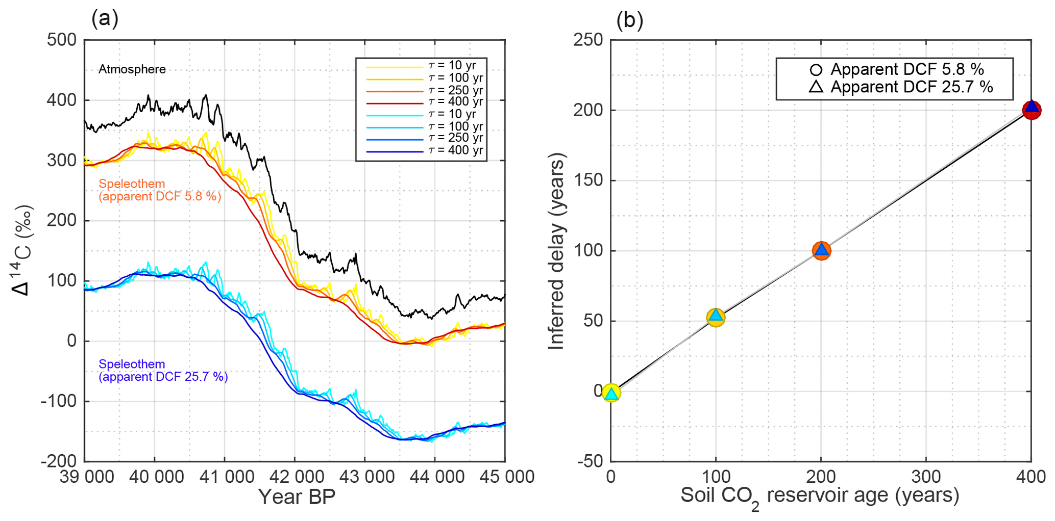
Figure 6 Effect of varying ages of soil respired CO₂ and fractions of CO₂ from ¹⁴C dead carbonate on the Δ¹⁴C in speleothems. (a) Atmospheric modeled Δ¹⁴C from the ¹⁰Be stack (black) and two modeled speleothem scenarios with a net DCF of 5.8 % (warm colors) and 25.7 % (cold colors). For each speleothem, a number of different ages for the respired soil organic matter have been assumed (see legend) and the input of ¹⁴C-free CO₂ from carbonate has been adjusted to obtain the correct apparent DCF value between 39 and 40.5 ka BP. (b) The inferred delay when we apply our synchronization method to match the atmospheric Δ¹⁴C to the speleothem record.

Table 1 Change-point detection window for each record. For each investigated climate event and record, the change-point detection algorithm has been applied between t1 and t2. The windows have been defined visually, ensuring a sufficient amount of data prior to and after the transition. For each record, only events that are well expressed in the climate proxy records at high resolution have been investigated. For the ice-core record, t1 and t2 typically encompass 500 years prior to and after the nominal transition ages by Rasmussen et al. (2014a). The exact values have been adjusted to exclude overlap with other transitions where necessary (Erhardt et al., 2018).

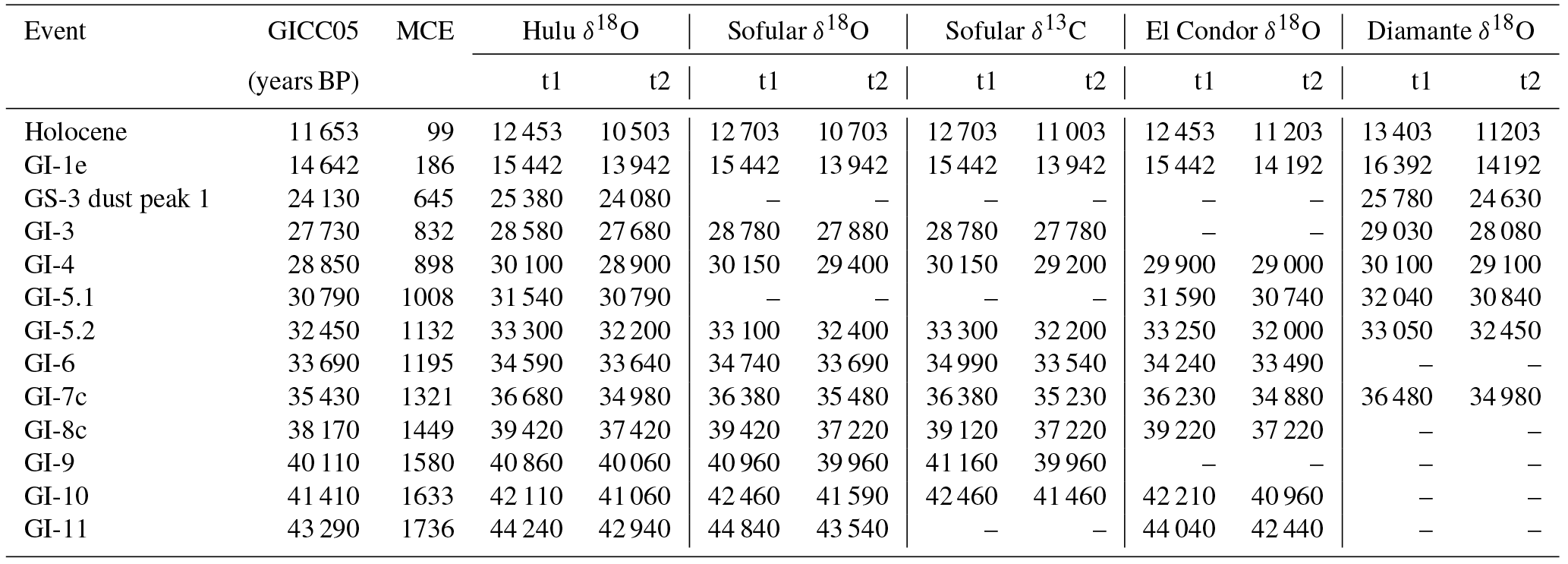
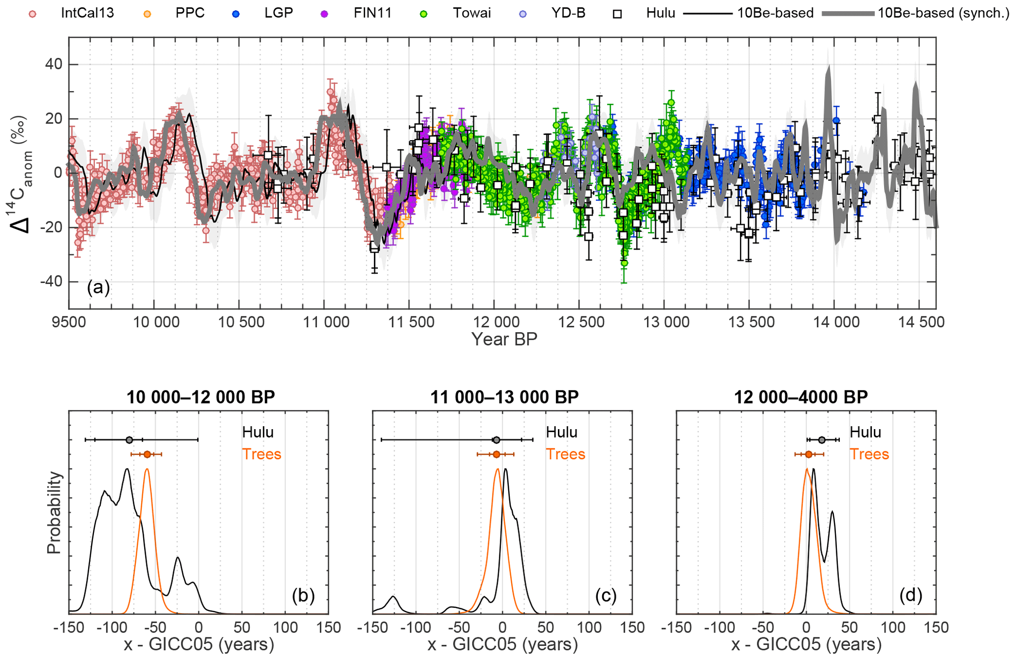
Figure 7 Synchronization of GICC05 to tree-ring and Hulu Cave records during the last deglaciation. (a) Ice-core-based modeled Δ¹⁴C anomalies on the original GICC05 timescale (thin black line, light grey shading encompasses the ±10 ‰ uncertainty (±1σ) of the modeled Δ¹⁴C based on the carbon cycle sensitivity experiments by Adolphi and Muscheler, 2016) and synchronized timescale (bold grey line). Tree-ring data underlying IntCal13 are shown in pink. Revised Northern Hemisphere tree-ring data according to Hogg et al. (2016) are shown in orange (preboreal pines), dark blue (late glacial pine), and light blue (Younger Dryas B chronology). New kauri Δ¹⁴C data by Hogg et al. (2016) are shown in purple (FIN11) and green (Towai). Hulu Cave H82 Δ¹⁴C data are shown as white squares. All symbols are shown with ±1σ error bars. All data are FFT filtered to isolate Δ¹⁴C variations on timescales < 1000 years. (b–d) Inferred probability distributions of timescale differences between GICC05 and tree rings (orange) and Hulu Cave (black). The symbols and error bars denote means and 68.2 % and 95.4 % confidence intervals of the inferred timescale difference. Each of the lower panels refers to a 2000-year subsection of the data indicated at the top of each panel.

3.5 Change-point detection in climate records

To test the synchroneity of rapid climate changes, we compare the timing of DO events seen in Greenland ice cores (Andersen et al., 2004) to a number of well-known U∕Th-dated speleothems that show DO-type variability from Hulu Cave (Cheng et al., 2016), Sofular Cave (Fleitmann et al., 2009), El Condor, and Cueva del Diamante (both Cheng et al., 2013b).

We use a probabilistic model to detect the onset, midpoint, and end of the rapid climate transitions in each individual record. The employed model describes the abrupt changes as a linear transition between two constant states. Any variability due to the long-term fluctuations of the climate records around the transition model is described by an AR(1) process that is estimated in conjunction with the transition model. The model is independently fitted to windows of data on their individual timescales (Table 1 and Fig. 13) around the rapid transitions. Inference was performed using Markov chain Monte Carl sampling (MCMC) to obtain PDFs of the timing of the onset, the length, and the amplitude of each transition in each record. Using these PDFs we can calculate delays of the onset, midpoint, and end of the climate transitions between different records, propagating the respective uncertainties of the parameters. For each record, only events that are well expressed and measured in high resolution have been fitted. The approach and inference procedure are described in more detail in Erhardt et al. (2018).

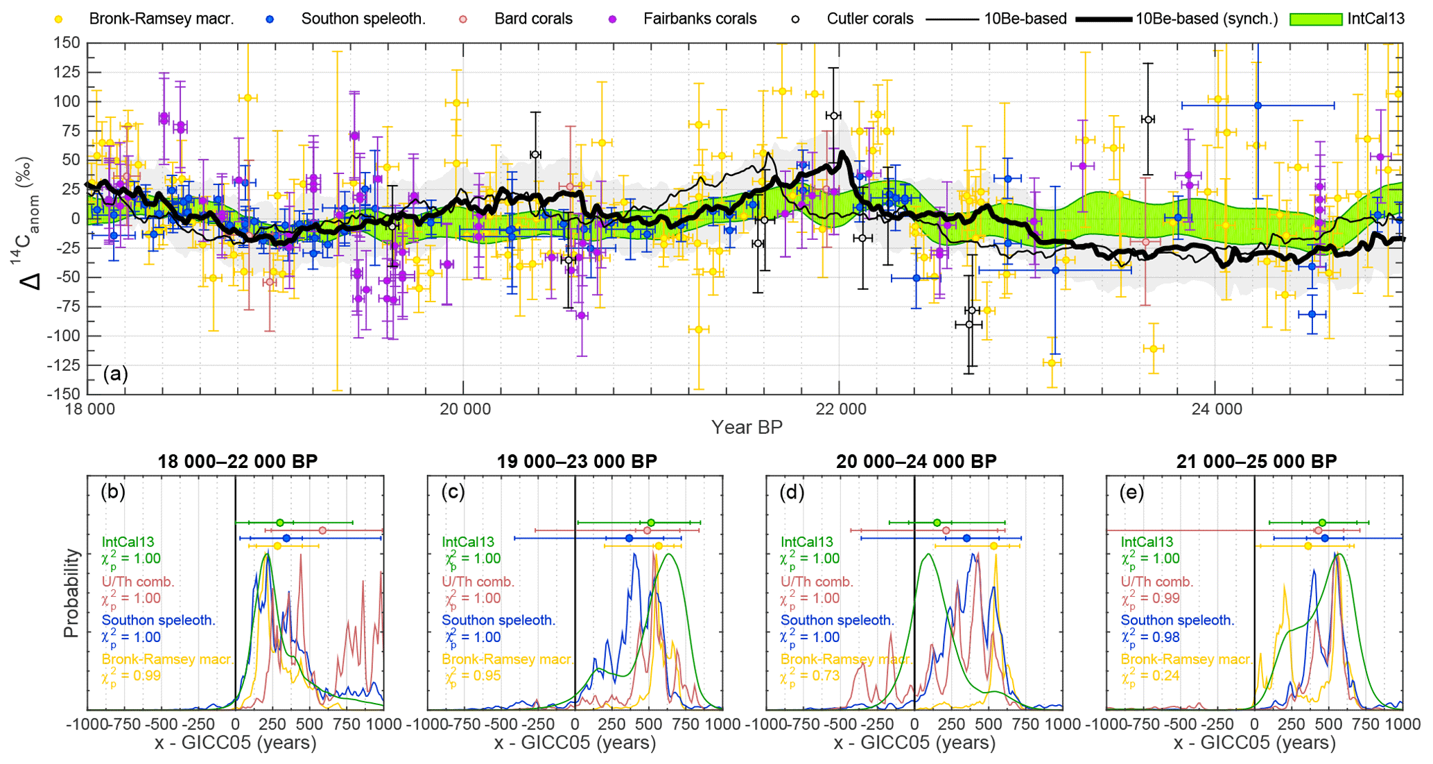
Figure 8 Synchronization results between 18 000 and 25 000 years BP. (a) The thin black line shows the modeled Δ¹⁴C curve based on the ice-core stack on its original timescale. The bold black line and grey shading show the synchronized ice-core record including assumed ±1σ uncertainties of ±30 ‰. The different colored symbols indicate various ¹⁴C datasets underlying IntCal13, which is shown as the green envelope. Lower panels: each panel shows PDFs of the inferred timescale difference between the ice-core stack and IntCal13 (green), a combination of all U∕Th-dated records (speleothems–corals, pink), the H82 speleothem (blue), and Lake Suigetsu (yellow). Symbols of similar color show the inferred mean and 68.2 % and 95.4 % confidence intervals. Color-coded text indicates χ² probabilities for the goodness of fit between modeled and measured Δ¹⁴C curves after synchronization. Small (e.g., < 0.1) values would indicate significant disagreement. Note that all χ² probabilities are relatively high, indicating that our uncertainty estimate for the modeled Δ¹⁴C is very conservative. Each of the lower panels refers to a specific subsection of the data indicated at the top of each panel.

4 Timescale differences between GICC05 and the U∕Th timescale

In the following sections we will show the synchronization results for different time windows. We focus our analysis on three distinct windows: 10–14, 18–25, and 39–45 ka BP. The youngest window is defined by the presence of high-resolution tree-ring data for ¹⁴C back to 14 ka BP. Going further back in time it becomes increasingly challenging to unequivocally identify common structures in the various Δ¹⁴C records that are suitable for synchronization because the resolution of the individual records decreases back in time, while their differences to each other grow steadily (see Fig. 1i). Hence, we focus on the well-known Laschamp event around 41 ka BP and the period between 18 and 25 ka BP, i.e., preceding the major carbon cycle changes associated with the deglaciation. We omit the period between 25 and 39 ka BP. As discussed in Reimer et al. (2013) and seen in Fig. 1i there is substantial disagreement between the datasets underlying IntCal13 at that time that are impossible to reconcile within their respective age and/or ¹⁴C uncertainties. Hence, any structure in the Δ¹⁴C records may also be unreliable and thus lead to erroneous synchronization results.

4.1 10 000–14 000 years BP

In the 10–14 ka BP interval, we synchronize the ice-core stack to high-resolution tree-ring and speleothem Δ¹⁴C data (Fig. 7). The high sampling resolution of the ¹⁴C records allows us to focus on centennial-to-millennial Δ¹⁴C changes (< 1000 years) for which carbon cycle influences on Δ¹⁴C can be expected to be small (Adolphi and Muscheler, 2016). In concordance with earlier studies (Muscheler et al., 2014a) we find that GICC05 is ∼65 years older than the tree-ring timescale at the onset of the Holocene, but that this offset vanishes over the course of the Younger Dryas interval.

While Muscheler et al. (2014a) argued that this changing offset may be in part due to errors in the timescale of the floating late glacial pines, we can now support this change in the timescale difference through the U∕Th-dated speleothems: the synchronization of the ice-core stack to the H82 speleothem from Hulu Cave (Southon et al., 2012) leads to fully consistent results as inferred from the tree rings. This indicates that the most likely explanation is an ice-core layer counting bias, i.e., that the GICC05 timescale suggests too-old ages at the onset of the Holocene, but is accurate within a few decades during GI-1.

Interestingly, we do not observe any significant differences between the results stemming from tree rings and the speleothem records. As shown in Sect. 3.4, we could expect a delay in the speleothem Δ¹⁴C compared to the atmosphere if the respired soil organic carbon contribution to the soil CO₂ was very old. This would result in GICC05 appearing older in comparison to the speleothem than relative to the tree rings. The lack of this delay implies that the majority of the respired soil organic carbon at Hulu Cave must be younger than ∼100 years (see Fig.  6). This is supported by the fact that the centennial Δ¹⁴C variations in the tree-ring and speleothem data have the same amplitude (Fig.  7). If old organic carbon significantly contributed to the soil CO₂, we would instead expect to see a stronger smoothing of short-term Δ¹⁴C variations.

4.2 18 000–25 000 years BP

Due to the irregular and lower sampling resolution of the ¹⁴C records beyond 15 000 cal BP, we chose to linearly detrend each dataset (instead of band-pass filtering) to remove offsets between the different ¹⁴C datasets (see Fig. 1i) and highlight common variability. Furthermore, we have to increase the length of the comparison data windows to 4000 years to ensure sufficient structure in the ¹⁴C sequences entering the comparison. Each window is detrended separately in the analysis to isolate short-term Δ¹⁴C variability. We note, however, that detrending each ¹⁴C dataset over the entire timeframe (18–25 ka BP) instead does not alter the results significantly. Compared to the high-frequency Δ¹⁴C changes studied between 10 and 14 ka BP, the longer-term variations used for synchronization here may have been increasingly affected by carbon cycle changes. To account for this, we increase the uncertainty estimate of the modeled Δ¹⁴C changes to ±30 ‰ (±1σ), which is sufficiently large to account for estimated carbon-cycle-driven Δ¹⁴C changes from modeling experiments during the entire glacial (Köhler et al., 2006). We note that this is a conservative estimate, given that during this period neither modeling (Köhler et al., 2006; Muscheler et al., 2004) nor data (Eggleston et al., 2016) suggest large carbon cycle changes.

It can be seen in Fig. 8 that it is challenging to infer robust covariability in multiple ¹⁴C records. However, the millennial evolution of Δ¹⁴C does show common changes in the 18–25 ka BP interval. Synchronizing the ice-core stack to data from (i) Hulu Cave H82 speleothem, (ii) Lake Suigetsu macrofossils, (iii) the IntCal13 stack, or (iv) a combination of all U∕Th-dated records (speleothems–corals) leads to consistent results within uncertainties for each choice of time windows: all records imply that GICC05 shows younger ages compared to the ¹⁴C records around this time.

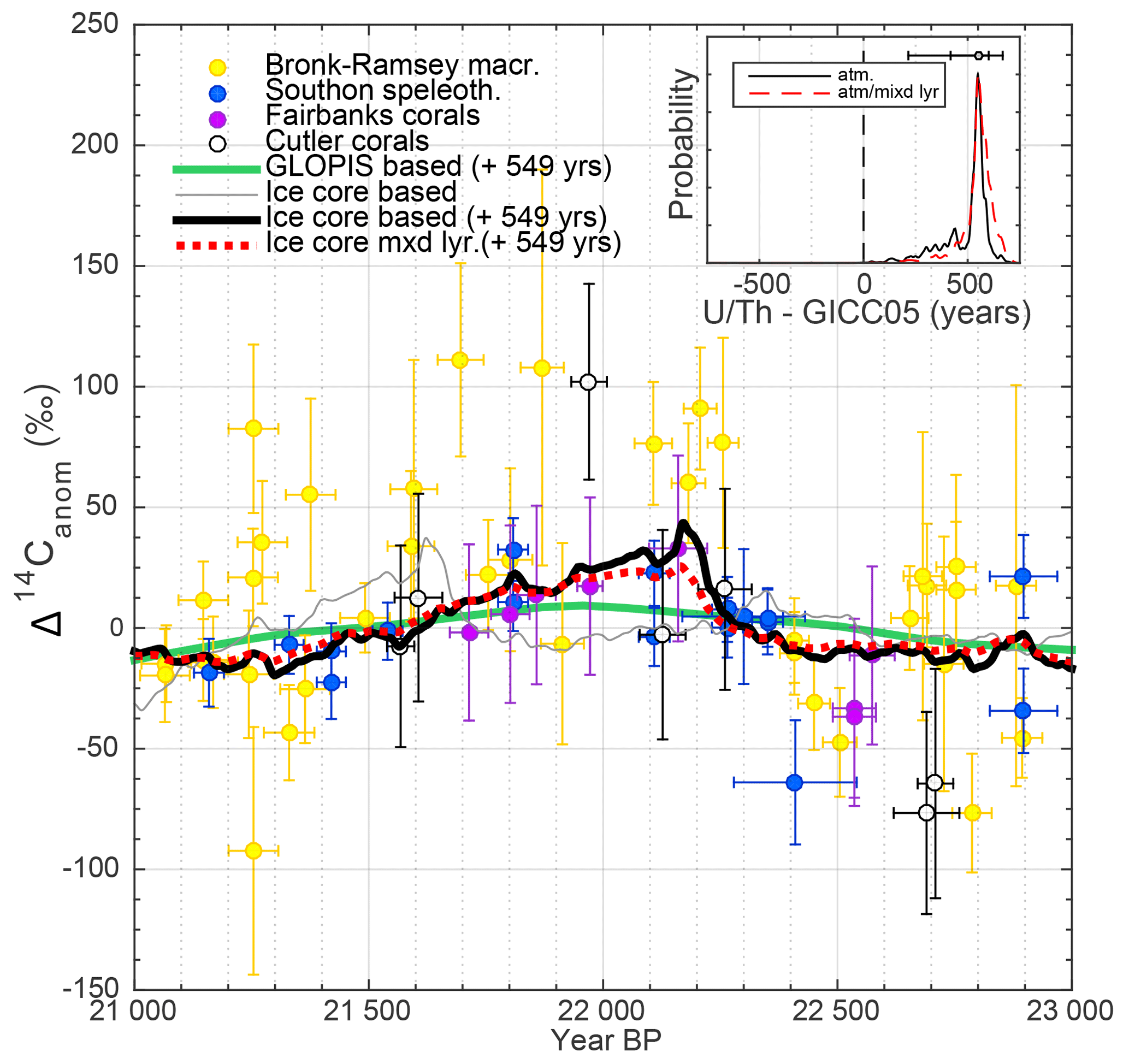
Figure 9 Close-up of measured and modeled Δ¹⁴C anomalies between 21 and 23 ka BP. The thin grey line shows modeled atmospheric Δ¹⁴C from the ice-core stack on the GICC05 timescale. The bold black and dashed red lines show the modeled atmospheric and ocean mixed layer Δ¹⁴C curves after synchronization to the ¹⁴C records (yellow: Lake Suigetsu; blue: Hulu Cave; purple and white: corals. The inset panel shows the PDF of the inferred timescale difference between GICC05 and the combination of all ¹⁴C records. The black line is based on using only the modeled atmospheric Δ¹⁴C. The red dashed line is based on comparing coral and speleothem data to the modeled mixed layer Δ¹⁴C and Lake Suigetsu data to modeled atmospheric Δ¹⁴C. The green line shows modeled Δ¹⁴C based on geomagnetic field changes.

The most significant structure that is present in all measured and modeled ¹⁴C records during this time is the centennial Δ¹⁴C increase around 22.1 ka BP (see Fig. 9). Comparing the ice-core stack to Δ¹⁴C between 21 and 23 ka BP indicates an offset of ∼550 years between GICC05 and the U∕Th timescale around this time (GICC05 being younger). To account for the potential delay of coral and speleothem Δ¹⁴C compared to the atmosphere, we also modeled the mixed layer Δ¹⁴C signal from the ice-core stack and synchronized this signal to the measured ¹⁴C data (Fig. 9). As discussed in Sect. 3.4, we find very little difference in the inferred timing since the Δ¹⁴C variation is relatively rapid (centuries). Comparing the Δ¹⁴C anomalies to geomagnetic field data shows that a small part of the longer-term development of this structure is probably driven by geomagnetic field changes. The amplitude (∼50 ‰) and short duration (centuries) of the Δ¹⁴C increase, however, suggest that this change is mainly driven by a series of strong solar minima comparable to the grand solar minimum period around the onset of the Younger Dryas (Muscheler et al., 2008). We used this tie point (Fig. 9) in the final synchronization as it is the best-defined feature in this time interval and consistent within error with the estimates shown in Fig. 8.

4.3 39 000–45 000 years BP

Our oldest tie point is the previously discussed Laschamp event around 41 ka BP. The only independently and absolutely dated ¹⁴C record around this time that has a sufficient sampling resolution is the Bahamas speleothem by Hoffmann et al. (2010). While offset in absolute Δ¹⁴C (see Fig. 1), the U∕Th-dated coral data support the amplitude and timing of the Δ¹⁴C increase seen in the speleothem even though precise synchronization is hampered by the low sampling resolution of the corals. The Lake Suigetsu record is characterized by large uncertainties and scatter around this time. As discussed in Sect. 3.3.2, IntCal13 is smoothed around Laschamp, having a smaller amplitude and a less sharp rise in Δ¹⁴C. For this tie point, we merely remove the error-weighted mean between 39 and 45 ka BP from each dataset, since detrending would remove the largest part of the signal. Hence, there are large Δ¹⁴C modeling uncertainties associated with unknown carbon cycle changes, and we assume a Gaussian ±1σ error of 50 ‰, which we consider conservative since sensitivity experiments imply that the impact of carbon cycle changes on Δ¹⁴C was likely below 40 ‰ (Köhler et al., 2006).

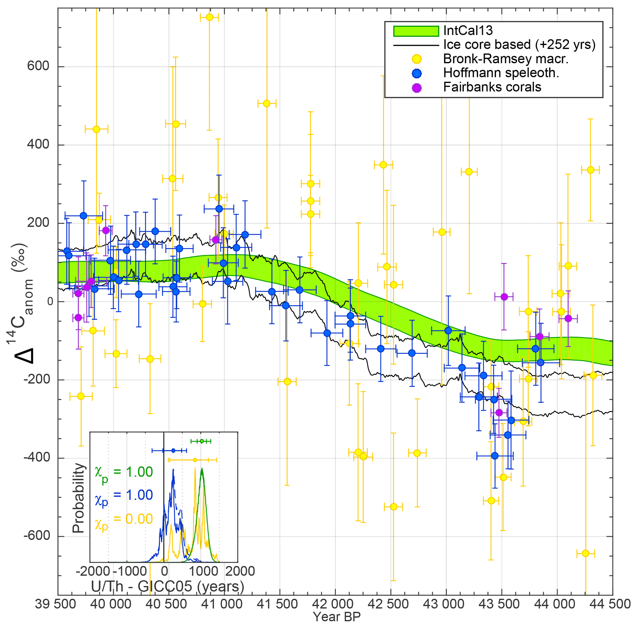
Figure 10 Synchronization of ¹⁰Be and ¹⁴C around the Laschamp event. The black lines encompass the modeled Δ¹⁴C anomalies (±1σ) from the ice-core data shifted by +252 years (68.2 % confidence interval = −103 to 477 years) according to their best fit to the speleothem ¹⁴C data. The green patch shows the ±1σ envelope of IntCal13. The blue and purple symbols show Δ¹⁴C from Bahamas speleothem and corals, respectively. The yellow symbols show Δ¹⁴C anomalies based on Lake Suigetsu macrofossils. All datasets have been centered to 0 ‰ by subtracting the error-weighted mean of each dataset. The inset shows the PDF of the inferred age differences between the ice-core data and IntCal13 (green), Lake Suigetsu (yellow), and the Bahamas speleothem (blue). The dashed blue line corresponds to age differences from the modeled mixed layer Δ¹⁴C and the Bahamas speleothem.

Synchronizing the ice-core stack to the speleothem, Lake Suigetsu, and IntCal13 data yields significantly different results. We infer that GICC05 produces ages about 250 years younger than the U∕Th-dated speleothem data (Fig. 10). The IntCal13 record, however, implies a larger difference of ∼1000 years. Using Lake Suigetsu data, on the other hand, leads to multiple probability peaks, two of which are in agreement with the speleothem and one with the IntCal13 record. The large scatter of the Lake Suigetsu data, however, leads to poor statistics (low χ² probabilities). Furthermore, the Lake Suigetsu timescale is only constrained by varve counting back to 39 ka BP and based on extrapolation for older sections (Bronk Ramsey et al., 2012); it hence provides less precise constraints on the timing of the Δ¹⁴C increase.

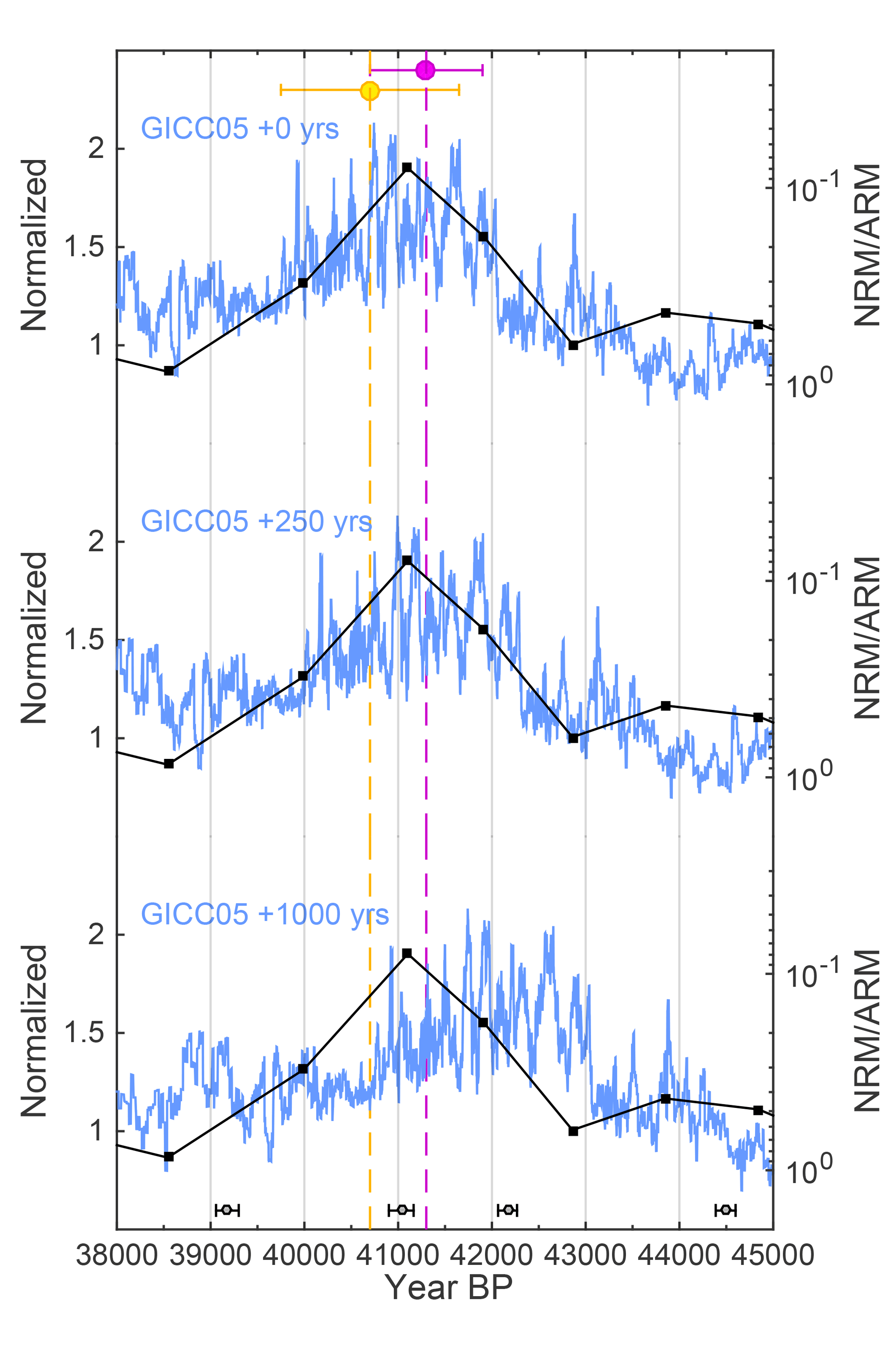
Figure 11 Comparison of the ice-core stack (blue) to Ar–Ar dates of the Laschamp excursion (yellow: Singer et al., 2009; pink: Laj et al., 2014) and relative geomagnetic field intensity (black; NRM/ARM; reversed y axis) from a U∕Th-dated speleothem (Lascu et al., 2016). The individual speleothem U∕Th dates are shown on the bottom of the figure with their ±2σ uncertainties. Each panel shows a different shift of GICC05 according to the results from Fig. 10.

To test which of these links is the most likely we turn to independent radiometric ages of the Laschamp excursion. Pooled Ar–Ar, K–Ar, and U∕Th ages on lava flows place the period of (nearly) reversed field direction at 40 700±950 years BP (Singer et al., 2009) or 41 300±600 years BP (Laj et al., 2014). In addition, a North American speleothem provides a U∕Th-dated transient evolution of the geomagnetic field (Lascu et al., 2016), with the lowest intensities occurring at 41 100±350 years BP. Comparing the ice-core ¹⁰Be stack to these data clearly shows that all of these records rule out the +1000 year time shift implied by IntCal13, as it would induce a significant disagreement between radiometrically dated magnetic field records and the dating of the ¹⁰Be peak in the ice cores (Fig. 11). We hence argue that the 252-year offset inferred from the comparison to the Bahamas speleothem is the most likely estimate of the timescale difference between GICC05 and the U∕Th timescale around this time. Similar to before, assuming that the speleothem represents a mixed layer signal instead of direct atmospheric Δ¹⁴C does not significantly affect the inferred timescale differences (see Fig. 10 inset, blue dashed line).

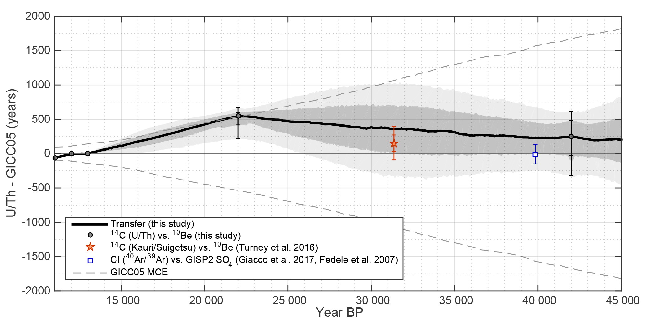
Figure 12 Transfer function between the U∕Th timescale and GICC05. The transfer function is shown in black with dark and light grey shading encompassing its 68.2 % and 95.4 % confidence intervals. The black dots with error bars show the match points used between ¹⁴C and ¹⁰Be. The red star shows the difference between ages of a glacial kauri tree ¹⁴C sequence on Lake Suigetsu ¹⁴C and GRIP ¹⁰Be (Turney et al., 2016). The blue open square shows the age difference between the ⁴⁰Ar∕³⁹Ar age of the Campanian Ignimbrite (Giaccio et al., 2017) and a tentatively associated spike in the GISP2 SO₄ record (Fedele et al., 2007) on the GICC05 timescale (Seierstad et al., 2014).

4.4 Transfer function

To construct a continuous transfer function between GICC05 and the U∕Th timescale we apply a Monte Carlo approach. Each iteration consists of (i) randomly sampling the PDFs at each tie point and (ii) interpolating between the tie points using an AR process that is constrained by the GICC05 maximum counting error (MCE). We use the tie points shown in Figs. 7, 9, and 10, i.e., three tie points between ice cores and tree rings during the deglaciation, one tie point between ice cores and the combination of corals, speleothems, and Lake Suigetsu during the LGM, and one tie point between ice cores and the Bahamas speleothem around the Laschamp event. For the interpolation, we use the time derivative of the MCE (i.e., its growth rate) as an incremental error estimate. During periods when the growth rate is > 0, GICC05 may be stretched (compressed), while a growth rate of 0 does not allow this, independent of what the absolute MCE is at that time. By multiplying this growth rate with a random realization of an AR process (Φ=0.9, σ=1), we simulate how much of that uncertainty has been realized in each iteration of the Monte Carlo simulation. Subsequently integrating over the resulting time series of simulated miscounts, we again obtain an absolute error estimate, i.e., one possible realization of the MCE. The parameters for the AR process were chosen so that the simulated realization of the MCE explores the whole absolute counting error space, without frequently exceeding the permitted growth rate of the MCE. A larger Φ would increase interpolation uncertainty, but also frequently violate the constraints of the layer count. A smaller Φ, on the other hand, would decrease the uncertainty due to shorter decorrelation length (see also the discussion in Rasmussen et al., 2006). In each iteration, this realization is then anchored at the sampled tie points (step i) by linearly correcting the offset between the sampled tie points and the simulated counting error. Hence, this procedure provides us with a correlated interpolation uncertainty over time, taking into account some of the constraints provided by the ice-core timescale itself, but giving priority to our inferred tie points. We note that this treatment of the MCE as an AR process leads to larger interpolation errors compared to assuming a white noise model, which would lead to very small uncertainties that average out over a long time (see also discussion in Rasmussen et al., 2006). Furthermore, we treat the MCE as ±1σ instead of ±2σ as proposed by Andersen et al. (2006), which additionally increases our interpolation error. We stress that this procedure does not aim to provide a realistic model of the ice-core layer counting process and its uncertainty, which is clearly more complex (see Andersen et al., 2006; Rasmussen et al., 2006), nor should it be interpreted such that the MCE was a 1σ uncertainty. However, our approach allows us to infer a conservative estimate of the interpolation uncertainty, while at the same time it takes advantage of the fact that GICC05 is a layer-counted timescale and hence cannot be stretched or compressed outside realistic bounds. This procedure was repeated 300 000 times, which was found sufficient to obtain a stationary solution leading to 300 000 possible timescale transfer functions.

Figure 12 shows the resulting mean transfer function along with its confidence intervals. First, it can be seen that all tie points fall into the uncertainty envelope of GICC05. The implied change in the timescale difference between the youngest two tie points (i.e., over the course of GS-1) and between 13 000 and 22 000 years BP is slightly larger than allowed by the MCE, although the latter is consistent within the uncertainties of the tie point at 22 000 years BP. We can see that the use of the MCE to determine the interpolation error leads to small uncertainties wherever the change in the timescale difference is large (e.g., over the 13 000–22 000 years BP interval): stretching GICC05 by as much as the counting error allows, requires that every uncertain layer has in fact been a real annual layer, leaving little room for additional error. Between 22 000 and 42 000 years BP, the interpolation uncertainties are determined by the MCE and thus grow or shrink at a rate determined by the MCE.

Our results are in very good agreement with the results by Turney et al. (2016) around Heinrich 3. In this study, a kauri-tree ¹⁴C sequence was calibrated onto Lake Suigetsu ¹⁴C and also matched on GICC05 via ¹⁰Be. The difference of the inferred ages (i.e., kauri on Suigetsu vs. kauri on GICC05) matches with our proposed transfer function (red star in Fig. 12).

Figure 12 also shows the inferred offset between the ⁴⁰Ar∕³⁹Ar age of the Campanian Ignimbrite (Giaccio et al., 2017) and a tentatively attributed SO₄ spike in the GISP2 ice core (Fedele et al., 2007). Even though it obviously requires a well-characterized tephra find in the ice cores to ensure that the SO₄ peak is indeed associated with the Campanian Ignimbrite, at least from a chronological point of view, our transfer function does not preclude this link. However, no matching shards were identified in this period (Bourne et al., 2013).

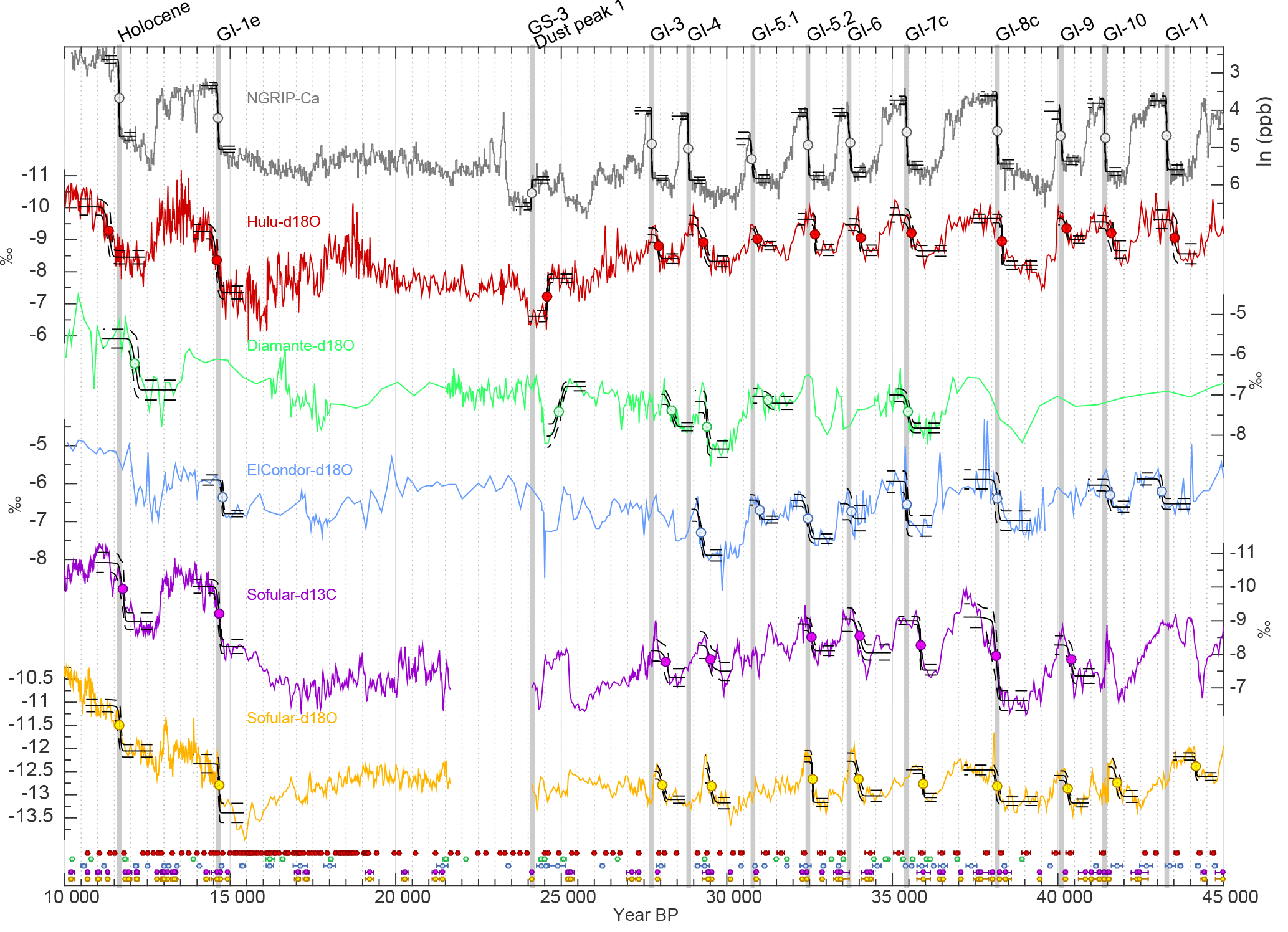
Figure 13 Timing of abrupt climate changes in different climate records. The climate archive and proxy are indicated in each panel. The black lines show the mean of the fitted ramps and their 95 % confidence intervals (dashed). The dots mark the midpoint of the mean transition. The U∕Th dates and their ±1σ uncertainties of each climate record are shown at the bottom of the figure in color coding corresponding to the respective climate record. Each time series is shown on its original timescale not applying any synchronization.

5 The timing of DO events

To investigate the synchroneity of climate changes recorded in different parts of the globe, we compare ice-core data to a selection of well-dated speleothem records. The well-known Hulu–Dongge Cave records have become iconic blueprints for intensity changes in the East Asian summer monsoon (EASM) anchored on a precise U∕Th timescale (Cheng et al., 2016; Dykoski et al., 2005; Wang et al., 2001). The speleothem records from Cueva del Diamante and El Condor reflect changes in precipitation amount over eastern Amazonia associated with the South American monsoon (Cheng et al., 2013b). The speleothem records from Sofular Cave, Turkey, are not straightforward in their mechanistic interpretation, but likely reflect a mix of temperature and seasonality of precipitation (δ¹⁸O), type and density of vegetation, soil microbial activity (δ¹³C), and hence effective moisture and temperature (Fleitmann et al., 2009). While this list of speleothem data can certainly be expanded in future studies, we chose these four speleothem records from three different regions that are all well dated and sensitive to the position of the ITCZ and compare it to the ice-core records. We used the NGRIP Ca record (Bigler, 2004), which shows the largest signal-to-noise ratio across DO events (compared to, e.g., δ¹⁸O), making their identification more precise. In addition, the Ca aerosols originate from Asian dust sources (Svensson et al., 2000) and are thus more directly related to Asian hydroclimate (Schüpbach et al., 2018), making them potentially more comparable to, for example, the Hulu Cave record. Potential phasing differences between different climate proxies in the ice core are small compared to our synchronization uncertainties (Steffensen et al., 2008).

Figure 14 Timing differences of the onset (a, b), midpoint (c, d), and end (e, f) of rapid climate changes in NGRIP and speleothems (colored PDFs; see legend) and the timescale transfer function inferred from radionuclide matching (black line and grey shadings as in Fig. 12). (a, c, e) The PDFs of timing differences including only uncertainties from the determination of the change points in the climate records; panels (b, d, f) also include the speleothem dating uncertainties.

Figure 13 shows the ice-core and speleothem climate records on their original individual timescales, along with the fitted ramps to the rapid climate changes. Note that we could not fit each climate event for every record, since the method requires a minimum number of data points defining the levels before and after each transition to produce reliable estimates. Already visually, a lag of climate changes in Greenland compared to the speleothem records can be consistently identified between 20 and 35 ka BP when all records are on their original timescales. Combining the PDFs of the detected change points in Greenland and the speleothems allows us to infer a probability estimate of the timing difference between climate events in Greenland and speleothems. These differences are shown in Fig. 14 along with our transfer function based on the matching of radionuclides from Fig. 12. This comparison shows that the differences in the timing of starting point, midpoint, and end point of DO events in speleothems and ice cores largely fall within the uncertainties of our radionuclide-based timescale transfer function. Thus, rapid climate changes occur synchronously in Greenland and the (sub)tropics. Notable exceptions are (i) the transition from GS-1 to the Holocene around 11.6 ka BP, (ii) Heinrich event 2 at 24 ka BP, and (iii) DO 11 around 43 ka BP. However, there is large scatter among the different speleothem-based estimates at these events, indicating that these events are asynchronous in the different speleothem records on their respective timescales. Consequently, some of these records also imply asynchronous climate shifts with Greenland ice cores. This may either be interpreted as an indication of time-transgressive climate changes or as a bias in individual speleothems either in how climate is recorded in the speleothem or their dating (for example, through detrital thorium).

Figure 15 Average lead–lag between the onset of DO events in the speleothems and NGRIP. Each panel (color) shows the PDF for the lead–lag of the onset in the speleothem compared to NGRIP, averaged over all investigated DO events (i.e., excluding the GS-3 dust peak, H2). Panel (f) shows the PDF of the average of all DO events and speleothems. The dark and light shading of the PDF in each panel indicates 68.2 % and 95.4 % intervals.

Averaging over all DO events, we can estimate an overall probability of leads and lags. By using the individual realizations of the radionuclide-based transfer function (see Sect. 4.4) we take into account that the uncertainties of the transfer function are strongly autocorrelated. For each realization, we randomly sample the PDFs for the onset of the DO events for the ice-core and speleothem records (see Sect. 3.5), perturb the speleothem-based estimates within their U∕Th dating errors, determine the lead or lag between the DO onset in ice-core and speleothem records, and correct it for the expected lag from the realization of our transfer function. By averaging over all DO events we thus obtain a mean lag for each realization and speleothem. In addition, we combine the different speleothem-based estimates of each realization by averaging over their mean lags to obtain an overall (speleothem and DO event) mean lag. Converting the obtained lags from each realization into histograms we estimate the PDFs of average lags between ice-core and speleothem records.

Our lag estimates critically depend on our ability to fill the gaps between the widely spaced tie points, and thus on our assumptions about the ice-core layer counting uncertainty, and how well our AR(1) process model can capture these (Sect. 4). However, we note that by treating the MCE as a highly correlated 1σ (instead of 2σ) uncertainty, our error estimate can be regarded as very conservative since it allows for large systematic drifts in each realization of the transfer function that will result in large errors of the mean.

The resulting PDFs of the lag between speleothems and ice cores are shown in Fig. 15. The uncertainties are mainly determined by our synchronization uncertainty. Thus, the uncertainty is only marginally reduced when averaging over all speleothems (Fig. 15, bottom). Because each realization of the transfer function varies smoothly, the offset between speleothem and ice-core records will be systematic for all speleothems in each realization and is thus only marginally reduced by averaging.

We find that all speleothem records except Cueva del Diamante (Cheng et al., 2013b) indicate synchroneity with NGRIP within 1σ and that the delay obtained for Cueva del Diamante falls within 2σ. We note that the speleothem data from El Condor (Cheng et al., 2013b) from the same region as Cueva del Diamante do not indicate a significant lag to Greenland. Overall, our analysis cannot reject the null hypothesis of synchronous DO events in Greenland ice cores and (sub)tropical speleothems (lag: $\mathit{\mu }\pm \mathrm{1}\mathit{\sigma }=\mathrm{26}\pm \mathrm{189}$ years).

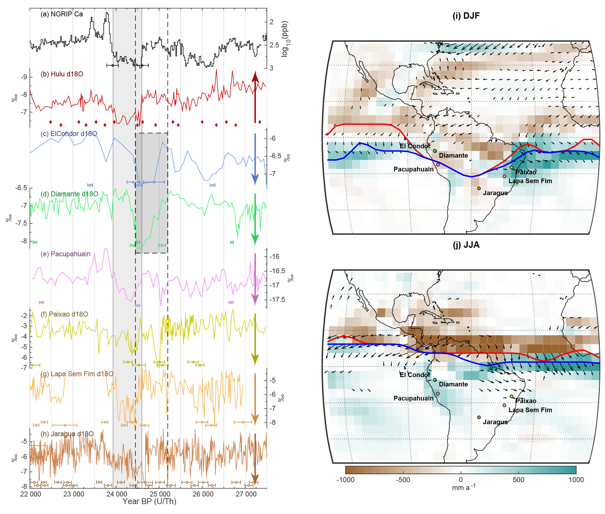
Figure 16 Climate changes around H2. (a–h) NGRIP Ca (Bigler, 2004) on the synchronized timescale (Fig. 14), Hulu Cave δ¹⁸O (Cheng et al., 2016), El Condor δ¹⁸O (Cheng et al., 2013b), Cueva del Diamante δ¹⁸O (Cheng et al., 2013b), (e) Pacupahuain δ¹⁸O (Kanner et al., 2012), Paixao δ¹⁸O (Stríkis et al., 2018), Lapa Sem Fim δ¹⁸O (Stríkis et al., 2018), and Jaragua Cave δ¹⁸O (Novello et al., 2017). The arrows on the right-hand side of each axis point in the direction of the signature of increased precipitation on δ¹⁸O through the amount effect (Dansgaard, 1964). The light grey box marks H2. The dark grey box highlights the preceding δ¹⁸O anomaly in El Condor and Diamante caves. (i, j) Precipitation (color) and wind (arrows) response to freshwater forcing in the CCSM3 climate model (freshwater-only experiment of TraCE21k, all other forcings are held at 19 ka BP conditions; He, 2011). The red (blue) line depicts the latitude of the precipitation maximum during strong (weak) AMOC states. Only wind anomalies > 1 m s⁻¹ are plotted. The cave sites are indicated as dots. Panel (i) shows the winter (December–February) response, while panel (j) shows the summer (June–August) response. Anomalies are plotted as weak–strong AMOC mode.

6 Discussion

Our proposed transfer function quantifies the long-term differences between the Greenland ice-core and U∕Th timescale and allows for their synchronization. Even though based on only a few tie points, this can be used to evaluate the absolute dating accuracy of Greenland ice-core records during the past 45 ka BP, while maintaining the strength of their precise relative dating. In combination with similar work done for the Holocene (Adolphi and Muscheler, 2016; Muscheler et al., 2014a), the picture emerges that the GICC05 counting error may be systematic: when accumulation and data resolution are high (e.g., in parts of the Holocene), too many annual layers have been counted, whereas during periods of low accumulation (e.g., GS-1 and GS-2) there is a tendency to identify too few annual layers. In principle, this is well captured by the GICC05 uncertainty estimate as the derivative of our transfer function is (within error) consistent with the increase in the counting error. However, our results caution against the use of the GICC05 counting error as a 2σ uncertainty as is often done in the literature. Originally, Andersen et al. (2006) pointed out that the MCE is not a true σ uncertainty but proposed that a Gaussian distribution with 2σ= MCE could serve as a pragmatic approximation. In combination with results from the Holocene (Adolphi and Muscheler, 2016) our study implies that the counting error can be strongly correlated over extended periods of time. This is in line with the discussion in Rasmussen et al. (2006), who point out that the main contribution to a potential bias in the layer count is the definition of how an annual layer is manifested in the proxy data. The data resolution and the manifestation of annual layers change between different climate states (Rasmussen et al., 2006), likely due to changes in aerosol transport and deposition resulting from variations in the atmospheric circulation and seasonality of precipitation (Merz et al., 2013; Werner et al., 2001). According to our analysis, the largest relative (i.e., year year⁻¹) change in the difference between GICC05 and the U∕Th and tree-ring timescale occurs over GS-1 (11 653–12 846 years BP) and GS-2 (14 652–23 290 years BP). Both of these periods have likely been characterized by an increased relative contribution of summer precipitation to the annual ice layer (Werner et al., 2000; Denton et al., 2005), and the annual layers in the ice core have been identified in a similar way in both intervals (Rasmussen et al., 2006). In the 11–13 ka BP interval, the offset between GICC05 and the tree-ring timescale changes from −60 (95.4 % range: −77 to −42) years to zero (95.4 % range: −12 to +21) years. During the same interval, the GICC05 maximum counting error grows by 46 years. Although consistent within the absolute error margins, this stretch of GICC05 over GS-1 thus slightly exceeds the range allowed by the GICC05 counting error. Muscheler et al. (2014a) discussed the fact that this stretch may be partly explained by errors in the placement of the oldest part of the tree-ring chronologies. However, here, we use a revised late glacial tree-ring dataset in which the different chronologies are connected much more robustly (Hogg et al., 2016). Furthermore, our analysis of the fully independent Hulu Cave ¹⁴C data yields similar results (Fig. 7). Hence, our analyses clearly show that the GS-1 interval is about 60 years too short in the GICC05 timescale.

Between 15 and 22 ka BP, our analysis yields a change in the GICC05 offset from +118 (95.4 % range: 2–220) years to +549 (95.4 % range: 207–670) years, while the GICC05 counting error grows by 335 years. Thus, again, our transfer function changes a little faster than the maximum counting error allows during this interval. We note that our ¹⁴C–¹⁰Be match point around 22 000 years BP has a relatively low signal-to-noise ratio in the ¹⁴C data (see Figs. 8–9) and should thus be regarded as tentative. However, as shown in Fig. 8 our results are generally robust against different choices of subsets of the ¹⁴C data and time windows. Nevertheless, it can also be seen that the estimates of the most likely age difference (i.e., the peak of the PDFs) differ slightly for different choices of ¹⁴C data. Hulu Cave yields a most likely offset of ∼325 years, while Suigetsu implies a bigger age difference of ∼550 years that coincides with a secondary probability peak in the Hulu Cave PDF. We note that assuming increased amounts of old soil organic carbon contributing to speleothem formation would lead to an even stronger difference between these estimates (see Sect. 3.4). Hence, we propose an age difference of +549 (95.4 % range: 207–670) years based on the combination of all data (Fig. 9) that is consistent within error with the estimates based on the single datasets shown in Fig. 8, but stress that this tie point should be reevaluated as new suitable ¹⁴C data become available in the future.

Assuming that the U∕Th dates are absolute, our transfer function can be used to account for the bias in the GICC05 timescale and thus facilitate comparisons of ice-core records to other absolutely dated archives. However, we note that our synchronization does not necessarily lead to consistent timescales with radiocarbon-dated records. As discussed in Sect. 3.3.2 (Fig. 4) and Sect. 4.3 (Figs. 10 and 11), discrepancies in the datasets underlying IntCal13 can lead to erroneous structures in the calibration curve. The reduced amplitude of the Δ¹⁴C change around the Laschamp geomagnetic field minimum in IntCal13 compared to its underlying data implies that IntCal Δ¹⁴C must be offset prior to and/or after the Laschamp event. This underlines the challenges in radiocarbon calibration around this time pointed out by Muscheler et al. (2014b). More recently, Giaccio et al. (2017) also pointed out that paired ⁴⁰Ar∕³⁹Ar and ¹⁴C dating of the Campanian Ignimbrite around 40 ka BP yields inconsistent ages when the ¹⁴C age is calibrated with IntCal13. Since IntCal13 in principle should be tied to the U∕Th age scale for sections older than 13.9 ka BP, this implies either an inconsistency between Ar∕Ar and U∕Th dating or in the reconstructed ¹⁴C levels of the calibration curve. The latter would be congruent with the conclusions by Muscheler et al. (2014b). If the problem was indeed the IntCal ¹⁴C reconstruction, a synchronization of ice-core ¹⁰Be to IntCal ¹⁴C would not resolve this bias, since the problem would not be one of chronology, but of ¹⁴C measurement and/or archive.

Our analysis provides the first rigorous test of whether DO events recorded in speleothems and ice cores occur synchronously. We reject the hypothesis of leads and lags larger than 189 years at the one sigma level, consistent with the findings of Baumgartner et al. (2014). Since we compare to speleothem records from different regions, this also highlights that the ITCZ likely migrated synchronously (within uncertainties) over the different ocean basins and continents during the onset of DO events (Schneider et al., 2014). However, there are also differences between the different speleothem records, which could be due to limitations in their dating or related to how directly individual archives record the rapid climate changes. The most notable examples are the onset of the Holocene and GI-11, which appear to occur asynchronously in the different speleothems (see Figs. 13 and 14). Another example is the younger GS-3 dust peak in the Greenland ice cores that appears to coincide with the East Asian summer monsoon decline seen in Hulu Cave, but postdates the precipitation increase seen in El Condor and Diamante. This change in the speleothems is typically attributed to the southward shift of the ITCZ as a response to Heinrich event 2.

Figure 16 shows the period around H2. First, we note that the younger of the two GS-3 dust peaks in the Greenland ice cores (Rasmussen et al., 2014a) occurs coevally (within chronological uncertainty) with the ITCZ movement recorded by the speleothems. At this time, the East Asian summer monsoon is strongly reduced as implied by decreased Hulu Cave δ¹⁸O (Cheng et al., 2016). Coevally, precipitation increases in the South American summer monsoon region (Novello et al., 2017; Stríkis et al., 2018). The records thus exhibit more pronounced stadial conditions than normally seen during (non-Heinrich) DO events. However, taken at face value, the precipitation increase at El Condor and Cueva del Diamante, the two northernmost sites shown in Fig. 16 (Cheng et al., 2013b), significantly predates the event seen in Greenland and Hulu Cave. It also predates the more southern South American sites Lapa Sem Fim (Stríkis et al., 2018) and Jaragua (Novello et al., 2017) by more than 500 years. This could either point to errors in the dating of the El Condor and Diamante speleothems or be related to their latitudinal position. A freshwater-only experiment (all other boundary conditions held constant at 19 ka BP levels) with the Community Climate System Model 3 (TraCE-MWF; He, 2011) shows that during a weak AMOC state, reduced advection of moisture from the tropical Atlantic leads to lower precipitation north of the ITCZ, while the ITCZ position over South America itself changes very little (Fig. 16). El Condor and Cueva del Diamante are both located very close to the LGM position of the ITCZ. It is hence possible that when Northern Hemisphere summer insolation reached its lowest values over the past 50 ka BP around H2, the ITCZ migrated to a position south of El Condor and Cueva del Diamante and during its transition caused the reconstructed precipitation change. As a result, the precipitation response to freshwater forcing would change sign at these cave sites. The sites located slightly further south only show a weak (Pacupahuain) or no (Paixao) response during this period, but are both characterized by increased variability. The two southernmost sites, on the other hand (Jaragua and Lapa Sem Fim), remain south of the ITCZ throughout and hence show a clear increase in precipitation coeval with the signal in Greenland and Hulu Cave. In this context, the precipitation increase in El Condor and Cueva del Diamante around 25 ka BP (i.e., prior to H2) may signify when the ITCZ transitions over the sites. The subsequent reduction in AMOC strength during H2 then leads to a decrease in precipitation in northwest South America, an increase further south, and little change in between. Tentative support for this can be drawn from the response of the El Condor and Cueva del Diamante speleothems to GI-2.2 and GI-2.1 for which, albeit weakly, the δ¹⁸O records imply an increase in precipitation during GI-2 opposite to their response to DO events during MIS-3 (Figs. 13, 16). Thus, this analysis indicates that the seemingly asynchronous response to climate change in different proxy records may indeed only reflect site-specific changes in the proxy response. Alternatively, we cannot rule out undetected issues with the U∕Th ages of these speleothems. A detailed analysis of this observation feature is beyond the scope of this paper, but in the context of a timescale perspective, which is the focus of this work, it highlights the caveats of climate wiggle matching between single records, even if the mechanistic link between regional climate changes may be relatively well understood.

7 Conclusion

We present the first radionuclide-based comparison between the Greenland Ice Core Chronology 2005 (GICC05) and the U∕Th timescale. We find that GICC05 is accurate within its stated absolute uncertainties, but also that the maximum counting error of the GICC05 may be at the limit to capture the total uncertainty accumulated within certain climatic periods. Our analysis indicates that the relationship between GICC05 and the U∕Th timescale over the last 45 ka drifts over time and reaches its maximum offset around 22 ka BP. We propose a transfer function that quantifies this drift and facilitates analysis of ice-core and U∕Th records, such as speleothems, on a common timescale. Thus, this transfer function allows for the further integration of key timescales in paleosciences and contributes to the INTIMATE (INTegration of Ice-core, MArine, and TEerrestrial records) initiative (Bjorck et al., 1996; Rasmussen et al., 2014b; Bronk Ramsey et al., 2014). Provided that U∕Th ages are regarded as accurate, the transfer function strongly reduces the absolute dating uncertainty of Greenland ice cores back to 45 ka BP. We reject the hypothesis of leads or lags larger than 189 years between Greenland, East Asia, and South America at the one sigma level. We show that the southward ITCZ shift around 24.5 ka BP seen in speleothems, typically associated with H2, coincides with the younger GS-3 dust peak recorded in Greenland ice cores. However, we also highlight inconsistencies between speleothem records around the onset of the Holocene, late GS-3, and GI-11 and thus caveats to the commonly applied practice of climate wiggle matching.

By comparing various ¹⁴C records underlying IntCal13 as well as ice-core ¹⁰Be data and geomagnetic field records, we infer that the current radiocarbon calibration curve underestimates the amplitude and rapidity of the Δ¹⁴C change around the Laschamp event at 41 ka BP. This adds to previous studies (Giaccio et al., 2017; Muscheler et al., 2014b) highlighting the fact that there are likely systematic errors in IntCal13 that will directly translate into errors of radiocarbon-based chronologies around that time. The combination of several internally inconsistent datasets in IntCal13 can lead to erroneous timing and amplitude of Δ¹⁴C changes. Hence, great care has to be taken when attempting to use sections older than 30 ka BP of IntCal13 directly for studies of ¹⁴C production rates and/or carbon cycle changes.