the Creative Commons Attribution 4.0 License.
the Creative Commons Attribution 4.0 License.
 | 12 Nov 2018
Link between the North Atlantic Oscillation and the surface mass balance components of the Greenland Ice Sheet under preindustrial and last interglacial climates: a study with a coupled global circulation model
Silvana Ramos Buarque
David Salas y Melia
The relationship between the surface mass balance (SMB) components (accumulation and melting) of the Greenland Ice Sheet (GrIS) and the North Atlantic Oscillation (NAO) is examined from numerical simulations performed with a new atmospheric stretched grid configuration of the Centre National de Recherches Météorologiques Coupled Model (CNRM-CM) version 5.2 under three periods: preindustrial climate, a warm phase (early Eemian, 130 ka BP) and a cool phase (late Eemian, 115 ka BP) of the last interglacial. The horizontal grid of the atmospheric component of CNRM-CM5.2 is stretched from the tilted pole on Baffin Bay (72∘ N, 65∘ W) in order to obtain a higher spatial resolution on Greenland. The correlation between simulated SMB anomalies averaged over Greenland and the NAO index is weak in winter and significant in summer (about 0.6 for the three periods). In summer, spatial correlations between the NAO index and SMB components display different patterns from one period to another. These differences are analyzed in terms of the respective influence of the positive and negative phases of the NAO on accumulation and melting. Accumulation in south Greenland is significantly correlated with the positive (negative) phase of the NAO in a warm (cold) climate. Under preindustrial and 115 ka BP climates, melting along the margins is more correlated with the positive phase of the NAO than with its negative phase, whereas at 130 ka BP it is more correlated with the negative phase of the NAO in north and northeast Greenland.
- Article
(10782 KB) - Full-text XML
-
Supplement
(2133 KB) - BibTeX
- EndNote


The recently observed acceleration of mass loss from the Greenland Ice Sheet (Hanna et al., 2013a, b; Fettweis et al., 2013b; Gillet-Chaulet et al., 2012, and references therein) is a concern due to its possible contribution to future sea-level rise. For example, Yan et al. (2014) estimated the Greenland Ice Sheet (GrIS) contribution to global sea-level rise by 2100 by means of ice-sheet model simulations (including dynamics) forced with output from 20 CMIP5 (Coupled Model Intercomparison Project phase 5) models to range from 0 to 16 (0 to 27) cm under the Representative Concentration Pathways (RCPs) 4.5 (RCP8.5). For a given RCP, this uncertainty is mainly due to the large spread among CMIP5 model simulations. Furthermore, Fürst et al. (2015) found that the largest source of uncertainty in projections of the GrIS contribution to sea-level rise arises from the surface mass balance (SMB) rather than from the dynamics of the ice sheet.
Since the early 1990s, the SMB of the GrIS has shown a downward trend due to increased surface melting (Ettema et al., 2009; Sasgen et al., 2012; Vernon et al., 2013). For example, during 12–15 July 2012, surface melting affected over 97 % of the GrIS (Nghiem et al., 2012; Dahl-Jensen et al., 2013), in the context of a negative phase of the North Atlantic Oscillation (NAO). Typically, this weather regime is associated with an anticyclonic circulation centered over Greenland that induces warmer and drier summers than normal and southerly warm air advection along the western Greenland coast at the surface and at 500 hPa. In recent years, changes in atmospheric circulation explain about 70 % of the summertime warming in Greenland (Fettweis et al., 2013a). Over the last 30 years, changes in the NAO index were found in winter and summer but not in spring and autumn (Hanna et al., 2015). In winter, the year-to-year climate and weather variability in Greenland and the North Atlantic region is captured well by the NAO index because the atmospheric circulation is active and well organized. By contrast, in summer, the NAO explains a smaller fraction of the circulation variability in this region (Folland et al., 2009).
On top of NAO changes, long-term climate change plays a role in the recent SMB trend. Climate change results from adjustments of the radiative forcing (arising from changes in atmospheric greenhouse gases and aerosol concentrations, and other factors), due to various radiative feedbacks (see, e.g., Geoffroy et al., 2013). In particular, in order to explain Arctic amplification, Pithan and Mauritsen (2014) quantified the contributions of these feedbacks in response to increasing atmospheric CO2 concentrations, based on CMIP5 climate model simulations. They found that the largest contribution arises from the surface temperature feedback rather than from the surface albedo feedback, because of the smaller increase in surface outgoing longwave radiation per degrees Celsius of warming at cold surface temperatures than at higher temperatures prevailing at lower latitudes.
In this paper, we focus on the link between NAO and SMB and its components (accumulation and melting) and its stability under the early and late periods of the last interglacial (Eemian) corresponding, respectively, to a warm and a cold climate. Such climate states can, to some extent, serve as analogs to interpret recent and future climate changes, but this is not the scope of this paper. Mechanisms of such changes can be studied by using coupled global circulation models (CGCMs). However, current CGCMs, that couple atmosphere–land surface and ocean–sea-ice models are increasingly comprehensive, but their typical horizontal resolution is currently around 100 km, which is too coarse to correctly represent local circulation in Greenland and surface moisture flux convergence. For example, snow sublimation is generally underestimated in CGCMs because the realism of this process highly depends on a good representation of the wind and especially on its maxima, which increase with resolution (Lenaerts et al., 2012). Ettema et al. (2009) have quantified SMB on the GrIS by using high-resolution (about 11 km) limited-area regional climate model simulations and found that considerably more mass accumulates than previously thought, revising upwards earlier estimates by as much as 63 %. This result highlights the need to use high-resolution models for estimating SMB. High resolution is also a necessary condition to capture well the spatial variability in the snowmelt on margins of the GrIS especially where snowmelt gradients are strong. This ability becomes all the more important as the expected trend in SMB in a warming climate is an enhanced melting along the GrIS margins. Hence, in order to locally increase horizontal resolution at a reasonable computational cost, in this study we use a stretched grid configuration (with enhanced resolution over Greenland) of the atmospheric component ARPEGE-Climat of the Centre National de Recherches Météorologiques Coupled Model (CNRM-CM).
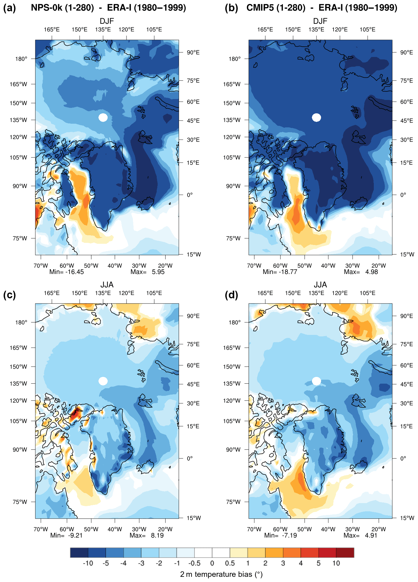
Figure 1Temperature biases at 2 m between the mean states from the preindustrial simulations (a, c) NPS-0k and (b, d) CMIP5 relative to the ERA-Interim (years 1980–1999) in (a, b) boreal winter (DJF) and (c, d) summer (JJA).
The questions addressed in this paper are the following. (i) What is the link between NAO variations and the variability in the GrIS SMB under preindustrial climate? (ii) How robust is this link under the warm and cool phases of the Eemian? (iii) What are the regions where SMB is most influenced by the NAO and to what extent is this the case? This paper is structured as follows. Section 2 describes the stretched grid configuration of CNRM-CM and the experimental design for this study. The preindustrial control simulation performed with CNRM-CM is analyzed in Sect. 3 and compared with the ECMWF Interim Re-Analysis (ERA-Interim) (Dee et al., 2011) and a previous CMIP5 simulation. The SMB and its link with NAO as simulated by CNRM-CM are compared with a simulation performed with MAR (Modèle Atmosphérique Régional). Section 4 is devoted to assessing the response of Greenland climate to large-scale changes under the warm (130 ka) and the cool (115 ka) phases of the Eemian, with a focus on summer.
2.1 Modeling tool
This study uses the CGCM CNRM-CM5.2 developed jointly by CNRM (Centre National de Recherches Météorologiques) and CERFACS (Centre Européen de Recherche et de Formation Avancée en Calcul Scientifique) as described by Voldoire et al. (2013). The components of CNRM-CM5.2 are the atmospheric model ARPEGE-Climat (Déqué et al., 1994), the surface platform SURFEX (Le Moigne et al., 2009), the river routing TRIP (Oki and Sud, 1998), the ocean model NEMO (Madec, 2008) and the sea ice model GELATO (Salas y Mélia, 2002). The components of CNRM-CM5.2 are coupled by means of the OASIS coupler (Valcke, 2006).
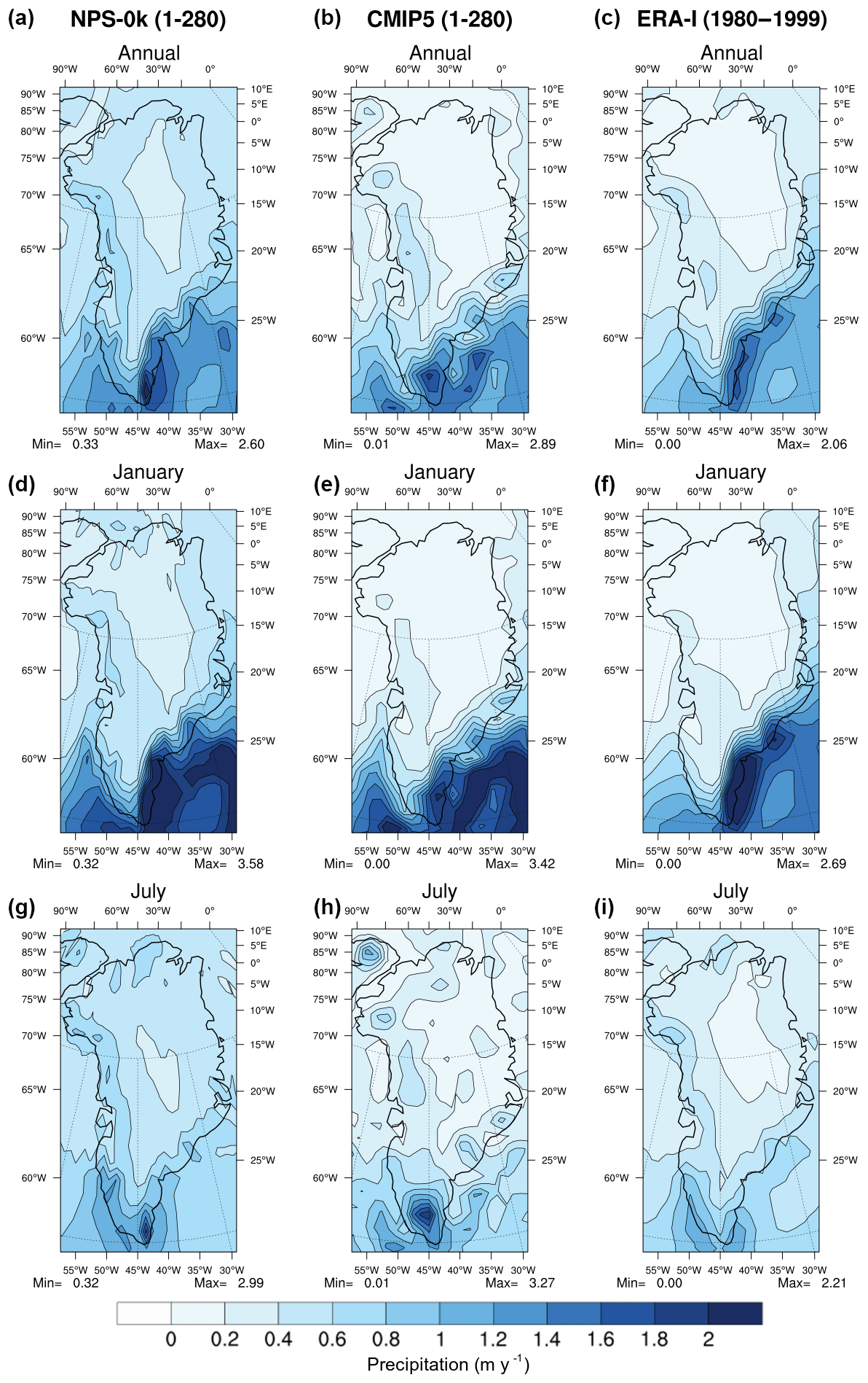
Figure 2Annual mean precipitation (a, b, c) and monthly mean precipitation for January (d, e, f) and July (g, h, i) in the preindustrial simulations (years 1–280) NPS-0k (a, d, g) and CMIP5 (b, e, h) and ERA-Interim (1980–1999) (c, f, i).
The ice mass transport due to the dynamics of the GrIS is not explicitly represented within CNRM-CM5.2. To circumvent this, the GrIS is represented by an initially prescribed huge amount of snow that evolves according to the balance between the snowfall rate, the direct sublimation and the snowmelt but without any modification of the topography of Greenland, the snowpack being represented by the one-layer snow scheme of Douville et al. (1995). This scheme has a restricted number of parameters preserving the surface energy budget. Prognostic equations for snow density and snow albedo account for the ageing process of the snowpack. To avoid unrealistic snow accumulation on the GrIS and an associated decrease in the modeled sea level, a pseudo-calving flux is computed at every time step from the spatially integrated snow reservoir excess over the GrIS and is distributed over the ocean north of 60∘ N
Table 1Astronomical forcing for all simulations after Berger (1978) in degrees.
* The precession is the longitude of the perihelion relative to the moving vernal equinox minus 180∘.
The atmospheric component ARPEGE-Climat is used in a “low-top” configuration with 31 vertical levels (the highest level is set to 10 hPa). The horizontal grid is defined by a T127 spectral triangular truncation (a global mean spatial resolution of about 150 km). In this study, however, we chose to increase horizontal resolution to 40–50 km over Greenland in order to improve the spatial representation of SMB, in particular near the GrIS margins. To do so, the North Pole of the ARPEGE-Climat horizontal grid was displaced to Baffin Bay (72∘ N, 65∘ W) and the grid was stretched by a factor of 2.5 following the spherical harmonic-based functions on a transformed sphere (Courtier and Geleyn, 1988). In the rest of this study, this configuration of CNRM-CM5.2 will be referred to as NPS (North Pole stretched). Different previous studies have used this functionality of increasing the horizontal resolution in a region of interest while decreasing it in other regions without any additional computational cost compared to a globally uniform resolution (e.g., Lorant and Royer, 2001; Doblas-Reyes, 2002; Chauvin et al., 2006). The physics and the calculations of the nonlinear terms require spectral transforms onto a reduced Gaussian grid (Hortal and Simmons, 1991).
The ocean component is deployed on the horizontal quasi-isotropic tripolar grid ORCA1 (Hewitt et al., 2011) with 42 vertical levels and a horizontal resolution of about 1∘. This grid has a latitudinal grid refinement of 1∕3∘ at the Equator, and the North Pole singularity is replaced by two poles located in Canada and Siberia.
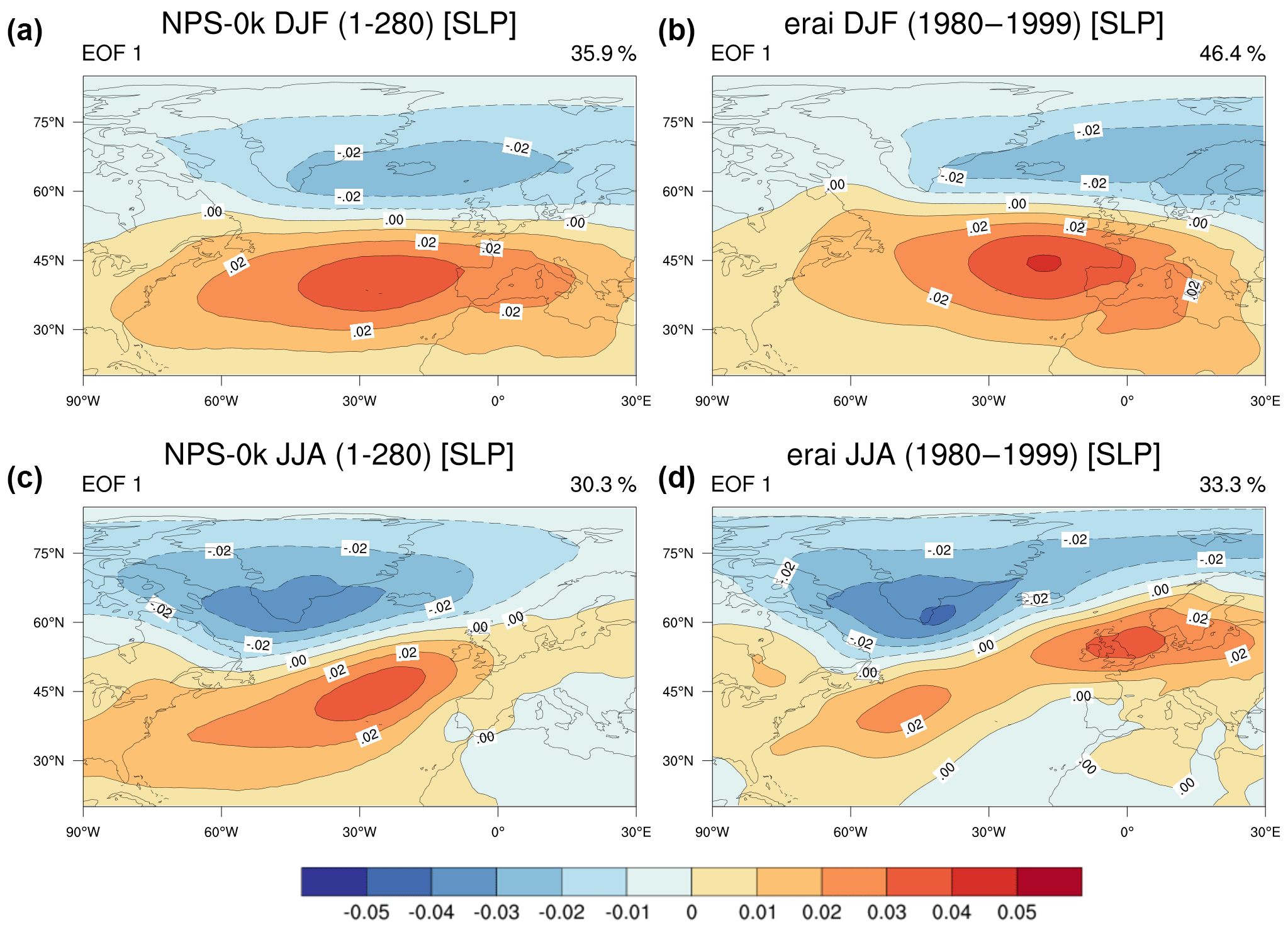
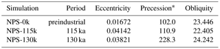
Figure 3Leading EOF of SLP for (a, c) NPS-0k (years 1–280) and (b, d) ERA-Interim (years 1980–1999) in winter (DJF, a, b) and in summer (JJA, c, d).
2.2 Experimental setup
Three 280-year simulations were performed with NPS: preindustrial (NPS-0k), early Eemian climate (130 ka, denoted as NPS-130k) and late Eemian climate (115 ka, denoted as NPS-115k). These simulations differ only by the astronomical parameters (orbital eccentricity, axial tilt, or precession and obliquity) that drive incoming insolation changes (Berger, 1988). In this study, we defined these parameters following Berger (1978) (see Table 1). In all the simulations, the concentrations of tropospheric aerosols (organic and black carbon, sea salt, sulfate and sand dust) are estimates from the LMDz-INCA chemistry–climate model (Szopa et al., 2013) for the years 1850–1860, considered as representative of preindustrial conditions. The atmospheric concentrations of well-mixed greenhouse gases (carbon dioxide, methane, nitrous oxide, ozone and chlorofluorocarbons (CFCs)) are yearly means for 1850. The 3-D stratospheric ozone concentration is averaged from the years 160–259 of the CMIP5 preindustrial control experiment run with CNRM-CM5.1. The solar constant is equal to 1365.6537 W m−2 for all the experiments, and the concentration of stratospheric aerosols produced by volcanic eruptions is a monthly zonal mean climatology derived from Ammann et al. (2003).
Atmospheric state variables (temperature, pressure, humidity and wind fields) were initialized from a previous forced integration of ARPEGE-Climat simulation. The initial states of NEMO and GELATO correspond to the first year of the CMIP5 preindustrial control experiment run with CNRM-CM5.1.
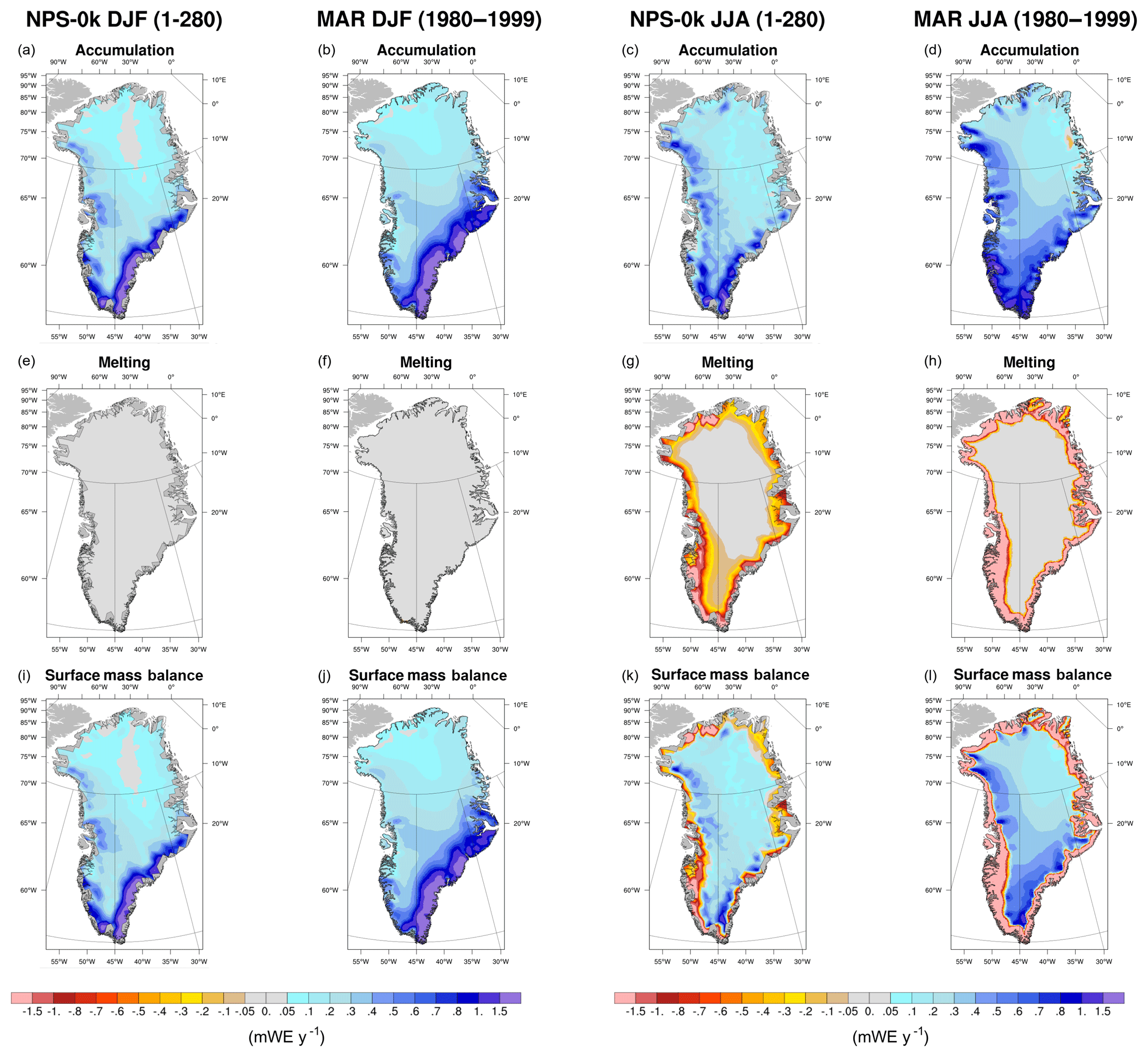
Figure 4Seasonal (DJF, left two columns and JJA, right two columns) mean accumulation (top row), melting (middle row) and SMB (bottom row) over Greenland from NPS-0k (a, c, e, g, i, k) and MAR (b, d, f, h, j, l).
The NPS-0k simulation was integrated for 280 years without discarding the spin-up since the model reaches a steady state soon after initialization. This is probably due to the fact that NPS-0k and CMIP5 preindustrial simulations essentially differ by their atmospheric horizontal grids. In the rest of this study, all the analyses of NPS will be based on the entire simulation.
Figure 5Seasonal (DJF, left two columns, and JJA, right two columns) correlations between the NAO index with mean accumulation (top row), melting (middle row) and SMB (bottom row) over Greenland from NPS-0k (a, c, e, g, i, k) and MAR (b, d, f, h, j, l).
The period 1980–1999 has been selected for all comparisons with preindustrial climate. This period corresponds to the beginning of the available MAR simulation we use and does not include the large melting events of 2007–2012 which are not typical of preindustrial climate.
3.1 Model evaluation
Differences between the simulated time-mean 2 m air temperature in the preindustrial experiments NPS-0k and CMIP5 (years 1–280) and ERA-Interim for winter (DJF) and summer (JJA) over the 1980–1999 period are plotted in Fig. 1. Note that these differences do not only depict model biases but also include the climate change signal since the preindustrial era.
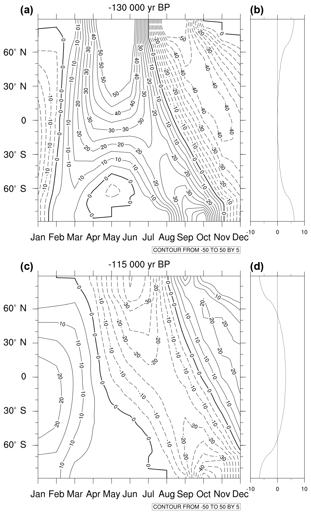
Figure 6Zonal mean departures of (a, c) monthly and (b, d) annual insolation from preindustrial conditions for (a, b) 130 and (c, d) 115 ka. On (a) and (c) contours are drawn every 5 W m−2 from −50 to 50 W m−2. Full lines are for positive deviations (Eemian values larger than preindustrial ones).
The Arctic is dominated by a cold bias that is much more pronounced in CMIP5 than NPS-0k in winter. The cold winter bias in the Greenland Sea already existed in CNRM-CM3 and remains in CNRM-CM5.2. Even if the geographical distribution of Arctic sea ice is generally well simulated by CNRM-CM5.2, particularly in winter, the ice edge in the Greenland and Barents seas does not match observations well (Voldoire et al., 2013). A weak (NPS-0k) to moderate (CMIP5) warm bias can be seen in Baffin Bay and the Labrador Sea. This bias is probably due to several coupled processes. A rough representation of turbulent surface heat and momentum fluxes and vertical turbulent mixing in the ocean and atmospheric boundary layers, particularly in their entrainment zones and stratified regimes, could be the causes, among others, of such biases. Biased kinetic energy transfers at the air–sea interface is also a potential source of oceanic biases because this coupled ocean–atmosphere process is particularly active in regions of strong currents (Giordani et al., 2013).
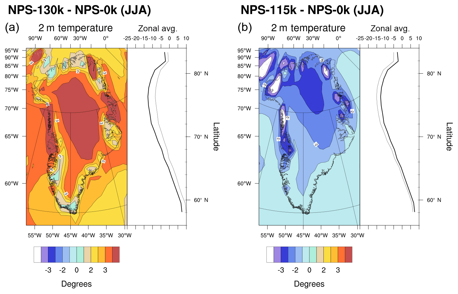
Figure 7Summer (JJA) 2 m temperature anomalies for 130 ka (a) and 115 ka (b) from preindustrial conditions. In both plots, the left and right subplots, respectively, represent the spatial pattern of anomalies and their zonal average.
In order to evaluate accumulation on the GrIS, the annual mean and monthly mean (January and July) precipitation simulated for NPS-0k, CMIP5 and ERA-Interim are plotted in Fig. 2. The simulated solid precipitation strongly depends on the model resolution, especially along the southeastern Greenland coast where the topography varies sharply over short distances and acts as a barrier for the atmospheric flow. The seasonal variations in precipitation over south and north Greenland are out of phase, with annual maximum values occurring, respectively, in January and July. In January, the mean precipitation in NPS-0k along the southeastern and southwestern Greenland coasts is similar to ERA-Interim. The improvement due to the higher horizontal resolution of NPS-0k compared with CMIP5 is clear for the representation of the highest annual precipitation (higher than 0.8 m WE yr−1) and of the distribution of precipitation along the coast. In July, the simulated precipitation in NPS-0k over south Greenland and along the western margin of the GrIS is very similar to ERA-Interim. Note that the most important contribution to the annual total precipitation is from July precipitation.
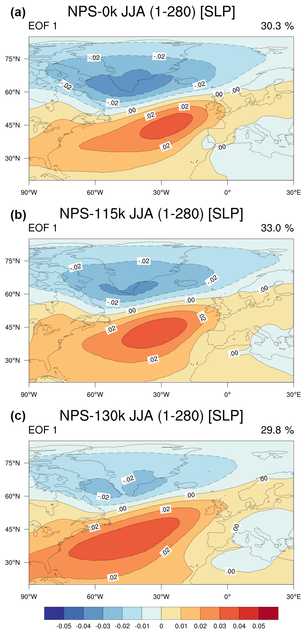
Figure 8Summertime (JJA) leading EOF of SLP for (a) NPS-0k, (b) NPS-115k and (c) NPS-130k (years 1–280).
The NAO index can be defined as the difference in sea-level atmospheric pressure between Lisbon (Portugal) or Ponta Delgada (Azores) and Stykkishólmur or Reykjavík (Iceland) (Hurrel, 1995). The drawback of this proxy is that it does not account for the fluctuations in the locations of the Icelandic Low and the Azores High. This implies that the NAO station-based index does not completely capture the seasonal, interannual and multidecadal spatial variability in the North Atlantic pressure patterns (Hanna et al., 2015). The NAO index can also be defined as the leading principal component (PC) of atmospheric pressure usually at sea level, 850 or 500 hPa. The associated empirically determined orthogonal function (EOF) provides the spatial structure of NAO (Björnsson and Venegas, 1997).
In this work, the NAO index is defined as the normalized PC associated with the first EOF (EOF1) of the detrended monthly sea-level pressure (SLP) anomalies in the North Atlantic (20–70∘ N; 90∘ W–40∘ E). Figure 3 shows the EOF1 for NPS-0k and ERA-Interim (1980–1999) in winter (DJF) and summer (JJA). In DJF, the positions of the simulated centers of action of NPS-0k are similar to those of ERA-Interim. In JJA, only the southern center of action in NPS-0k reveals a slight southwestward shift compared to ERA-Interim. The EOF1 of NPS-0k and ERA-Interim explain, respectively, 35.9 % and 50.3 % of the total variance in SLP in DJF and 30.3 % and 36.2 % in JJA.
3.2 Simulated mean states
The SMB can be written as
where P, E and M (all positive), respectively, represent snowfall, the sublimation of the snowpack and surface melting. Figure 4 compares accumulation , melting M and SMB diagnosed from NPS-0k with their counterparts simulated by MAR for the period 1980–1999, which serves as a reference. The latter simulation was performed with MAR version 3.2 (Fettweis et al., 2013b) at a horizontal resolution of 25 km and was driven by ERA-Interim at its lateral boundary conditions.
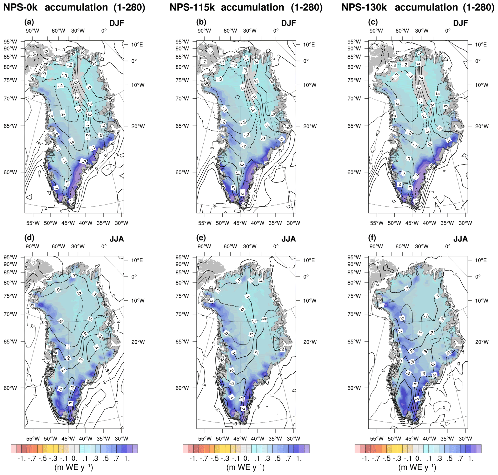
Figure 9Mean accumulation (in m WE yr−1) and (superimposed) its correlation with the NAO index for (a, d) the preindustrial period, (b, e) 130 ka and (c, f) 115 ka in (a, b, c) winter and (d, e, f) summer.
NPS-0k and MAR accumulations (Fig. 4a–d) compare well. Three regions of accumulation were identified in these simulations. A “dry” region in central and northeast Greenland, where C is less than 0.2 m yr−1, a “wet” region along the southeastern and southwestern margins of the GrIS where C is greater than 1 m yr−1, and the rest of Greenland where accumulation is intermediate. NPS-0k reproduces quite well the wet zone simulated by MAR thanks to its relatively high resolution.
In NPS-0k, the simulated melting rates are underestimated along the margins, especially in the southwestern part of the GrIS, south of the Jakobshavn region. MAR displays much higher melting rates along the margins (Fig. 4g–h). Melting is underestimated in NPS-0k mainly because in CNRM-CM5.2 the minimum albedo of permanent ice is set to 0.8, which hampers the feedback between albedo, solar radiation absorption and melting. The simpler representation of snow in CNRM-CM5.2 compared to MAR may also partly explain this bias. Indeed, MAR includes the physically based surface scheme SISVAT (Soil Ice Snow Vegetation Atmosphere Transfer) accounting for refreezing and percolation of meltwater and snow settling (Gallée and Duynkerke, 1997). Moreover, even at a horizontal resolution of 50 km, the relatively steep topography of the GrIS near the margins cannot be correctly represented, which probably also contributes to the biased simulated surface melting in this area.
Even if the melting in NPS-0k is strongly underestimated (Fig. 4g–h), the simulated equilibrium line, which separates the accumulation zone from the ablation zone, is fairly realistic (Fig. 4k). In the dry region, NPS-0k and MAR display slightly positive SMBs (< 0.2 m WE yr−1). All in all, the SMB is reasonably represented in the NPS-0k simulation compared to the reference MAR.
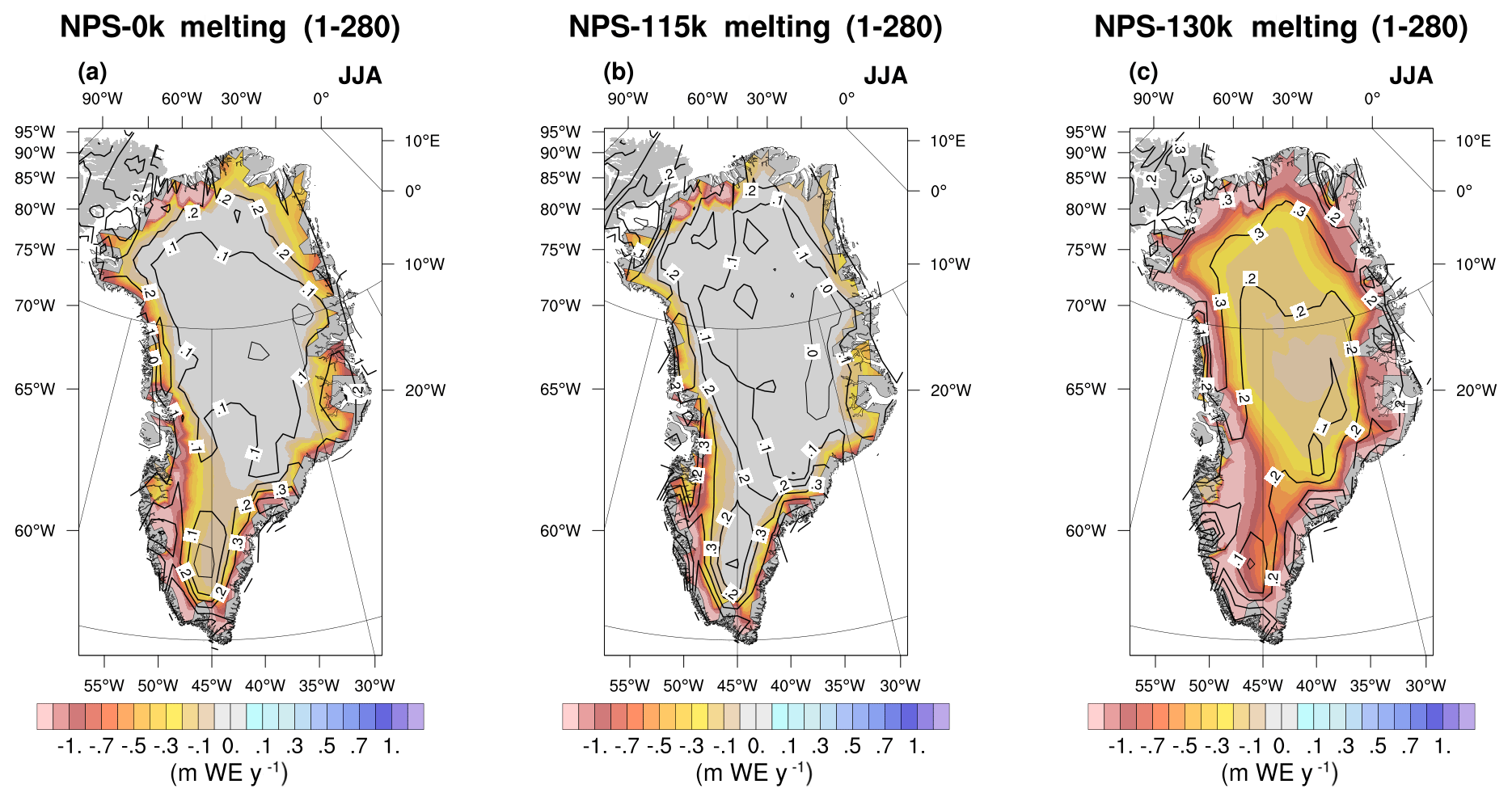
Figure 10Summertime mean melting (in m WE yr−1) and (superimposed) its correlation with the NAO index for (a) the preindustrial period, (b) 130 ka and (c) 115 ka.
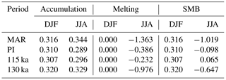
GrIS-averaged seasonal accumulation, melting and SMB for NPS-0k and MAR are presented in Table 2. These spatial integrations were computed after interpolating output from both models on a rectilinear grid and masked over the same exogenous Greenland mask obtained from the Global Database of Administrative areas (GADM, http://www.gadm.org, last access: 2 November 2018). In DJF, the mean accumulation averaged on the GrIS in NPS-0k is in close agreement with MAR (0.31 and 0.32 m WE yr−1, respectively), whereas in JJA, it is lower in NPS-0k than in MAR (0.29 and 0.34 m WE yr−1 in JJA). A comparison with MAR confirms that, as expected, the GrIS-averaged simulated melting in NPS-0k is greatly underestimated. However, even in NPS-0k, melting exceeds accumulation on the GrIS.

Figure 11Spatial correlation between accumulation and the NAO index in winter for (a, d) the preindustrial period, (b, e) 115 ka and (c, f) 130 ka. Top (bottom) row: positive (negative) NAO situations (sampled for NAO indices with absolute value higher than 1 standard deviation). Dotted areas represent correlations significant at the 99 % level.
3.3 Relationship between the interannual variability in NAO, GrIS SMB and its components
We compute the NAO index from ERA-Interim since this reanalysis is the lateral boundary condition of the MAR regional simulation (1980–1999) period that we used as a reference to validate SMB and its components. Note, however, that correlation estimates from MAR and ERA-Interim are probably not robust due to the short time series used (20 years).
Table 2Winter (DJF) and summer (JJA) mean accumulation, melting and SMB averaged on the GrIS for the MAR (1980–1999) simulation and for the NPS simulations in the preindustrial period, at 115 ka and at 130 ka (years 1–280). Units are in m WE yr−1.
First, we study the correlation between the NAO index and the time-detrended GrIS-averaged SMB. In order to investigate the stability of these correlations over time, we calculated them for 14 consecutive chunks of 20 years extracted from the NPS-0k simulation. For the 20-year time spans in NPS-0k, correlations range from −0.47 to 0.06 in winter and from 0.44 to 0.73 in summer. These results are compatible with correlations of −0.21 in winter and 0.40 in summer computed from MAR and ERA-Interim for 1980–1999. In winter, the correlation computed over the entire 280-year NPS-0k simulation is slightly negative (−0.22) and comparable with MAR, meaning that a positive NAO index is preferably (but not systematically) associated with SMBs lower than average. In summer, SMB anomalies are more strongly correlated with the NAO index (0.62) than in the MAR simulation.
Maps of seasonal correlations of the NAO index with accumulation, melting and SMB are shown in Fig. 5 for NPS-0k and MAR. For both seasons (DJF and JJA), the correlation maps are broadly consistent between the two models but generally stronger in MAR. Correlations computed from MAR display more small-scale patterns than those from NPS-0k. This probably mirrors both the higher spatial resolution and the short simulation period of MAR. In winter, accumulation is negatively correlated to the NAO index along a band stretching from northwestern to southeastern Greenland (Fig. 5a–b). This analysis also holds for SMB, since there is virtually no melting in winter (Fig. 5i–j).
4.1 Changes in solar radiation and climate response
The orbital eccentricity, precession and obliquity modulate the solar flux at the top of the Earth's atmosphere. The eccentricity is the deviation of the orbit from a perfect circle and is the only orbital parameter that can modify the global-year mean solar irradiance per unit surface area. The precession is the change in the orientation of the Earth's rotational axis and the obliquity is the angle between the Earth's rotational axis and its orbital axis. Both parameters alter the distribution of solar energy by latitude bands. The eccentricity and precession parameters mainly modulate the Earth–Sun distance, whereas obliquity mainly determines the latitude with the largest solar irradiance. During the Eemian, changes in precession compared to the preindustrial period led to significant insolation changes due to the high eccentricity. On top of that, high (low) obliquity is associated with less (more) insolation at middle and high latitudes. Hence, since the obliquity increases with time from the beginning (130 ka) to the end (115 ka) of the interglacial period, high latitudes received less irradiation at 115 ka than at 130 ka.
Zonal averages of monthly and annual insolation anomalies between the Eemian and the preindustrial periods are shown in Fig. 6. The 130 ka period is characterized by positive annual anomalies at high latitudes with very different seasonal cycles between the Northern Hemisphere (NH) and the Southern Hemisphere (SH). Strong positive anomalies (> 50 W m−2) prevail north of 20∘ N during approximately 2 months (April–May) whereas in the Southern Hemisphere positive anomalies only appear south of 60∘ S during approximately 1 month. In tropical regions, anomalies are negative for 6 consecutive months and the annual mean insolation anomaly is close to 0. At 115 ka, insolation anomalies broadly have the opposite signs compared to those of 130 ka. More (less) solar energy reaches tropical (polar) regions for 115 ka than for 130 ka. The monthly gradient of insolation anomaly during spring and autumn decreases between 130 and 115 ka. The Earth's orbital parameters lead to zonal annual changes in insolation from the preindustrial period that depend on the seasonality of solar radiation. In the Arctic, the annual increase (decrease) in insolation anomalies at 130 ka (115 ka) compared to the preindustrial period results in a warmer (cooler) climate from March to June (April to July). In order to document the near-surface response to the changes in insolation, the simulated NPS-130k and NPS-115k 2 m temperature summertime anomalies (with reference to NPS-0k simulation) are plotted in Fig. 7. The three NPS experiments only differ by the orbital parameters, and therefore changes in mean states and variability can be attributed to differences in solar forcing. In NPS-130k, the largest positive 2 m temperature anomalies, as high as 4 ∘C, appear in the central part of the GrIS (Fig. 7a), where the high elevation leads to cold and dry conditions. This anomaly suggests that in this region the ice sheet and atmosphere interact through a thermodynamic balance. In this region, the mean circulation is mostly controlled by local processes. Conversely, in NPS-115k, the largest cooling anomalies do not correspond with the highest elevations, suggesting that even in the central part of the GrIS, the mean climate is mainly determined by atmospheric dynamics rather than local processes. The largest negative temperature anomalies occur in the northern part of central Greenland (Fig. 7b), which are influenced by cold northerly winds blowing from the ice-covered Arctic Ocean to Greenland, cooling the near-surface atmosphere.
We finally examine changes in the seasonal (DJF and JJA) means of accumulation, melting and SMB averaged over the Greenland mask for interglacial and preindustrial climates (Table 2). In contrast with MAR, there is less accumulation in summer than in winter under all climates. Since accumulation increases with temperature, the accumulation is stronger at 130 ka for both seasons. Even if simulated melting rates are underestimated, since the same model is used for all experiments, we compare them in terms of relative values. As a consequence of obliquity changes, melting is much larger at 130 ka than for the preindustrial period and 115 ka.
The spatial structure of the NAO patterns does not depend much on the considered period, as shown in Fig. 8. The southern positive node extends farther west and south during 130 ka, and the extension of the northern negative node is smaller at 130 ka than at 115 ka and the preindustrial period. The total variance in SLP explained by EOF1 does not depend much either on the period and is equal to 30.3 %, 33.0 % and 29.8 %, respectively, in NPS-0k, NPS-115k and NPS-130k.
4.2 The link between NAO and SMB components
Correlation maps between SMB components and the NAO index for the preindustrial period and both interglacial climates are plotted in Figs. 9 (accumulation) and 10 (melting).
In winter (Fig. 9a–c), the overall similarity of the patterns of accumulation and their correlation with the NAO index for all climates suggests that variations in zonal annual insolation do not significantly modulate accumulation or atmospheric circulation. The correlation maps show that the link between the NAO index and accumulation is relatively strong under all climates in the northwestern (negative correlations) and northeastern (positive correlations) parts of the central GrIS. Correlations are negative in the northwestern part of central Greenland and are slightly positive in south Greenland particularly at 115 and 130 ka. In summer (Fig. 9d–f), there is slightly more accumulation at 130 ka than at 115 ka or the preindustrial period, which is confirmed by the GrIS-averaged values provided in Table 2. Correlation coefficients are overall positive, increasing from northwestern central Greenland (dry zone) towards the coast. The strongest correlations are confined to the southwestern GrIS reflecting increased snow precipitation at low elevations during the positive phase of the NAO, when the atmospheric flow is more pronounced. More inland, strong correlations are due to the barrier effect of the GrIS that forces the rise in atmospheric moisture and subsequent snow precipitation (Bromwich et al., 1999; Folland et al., 2009; Fettweis et al., 2011; Auger et al., 2017).
Since there is virtually no melting in winter, melting and its correlation with the NAO index are only shown for summer (Fig. 10). The preindustrial melting pattern (Fig. 10a) is intermediate between 115 ka (Fig. 10b) and 130 ka (Fig. 10c). Correlation coefficients tend to be higher along the coasts than inland. At 130 ka, the large mid- to high-latitude warming explains the wide band with melting along the GrIS margins. In particular, strong melting occurs in the northeastern part of the GrIS (Fig. 10c), suggesting this area to be a vulnerable part of the GrIS under a warm climate, since accumulation does not compensate for melting (Fig. 9d). Similarly, Born and Nisancioglu (2012) concluded that at 126 ka, the strongly negative annual mean SMB in the northeastern part of the GrIS leads to a significant thinning of the ice sheet, which is amplified by the ice elevation feedback. Overall, on the margins of the GrIS the cold climate does not inhibit melting.
4.3 Impact of the NAO phases on accumulation and melting
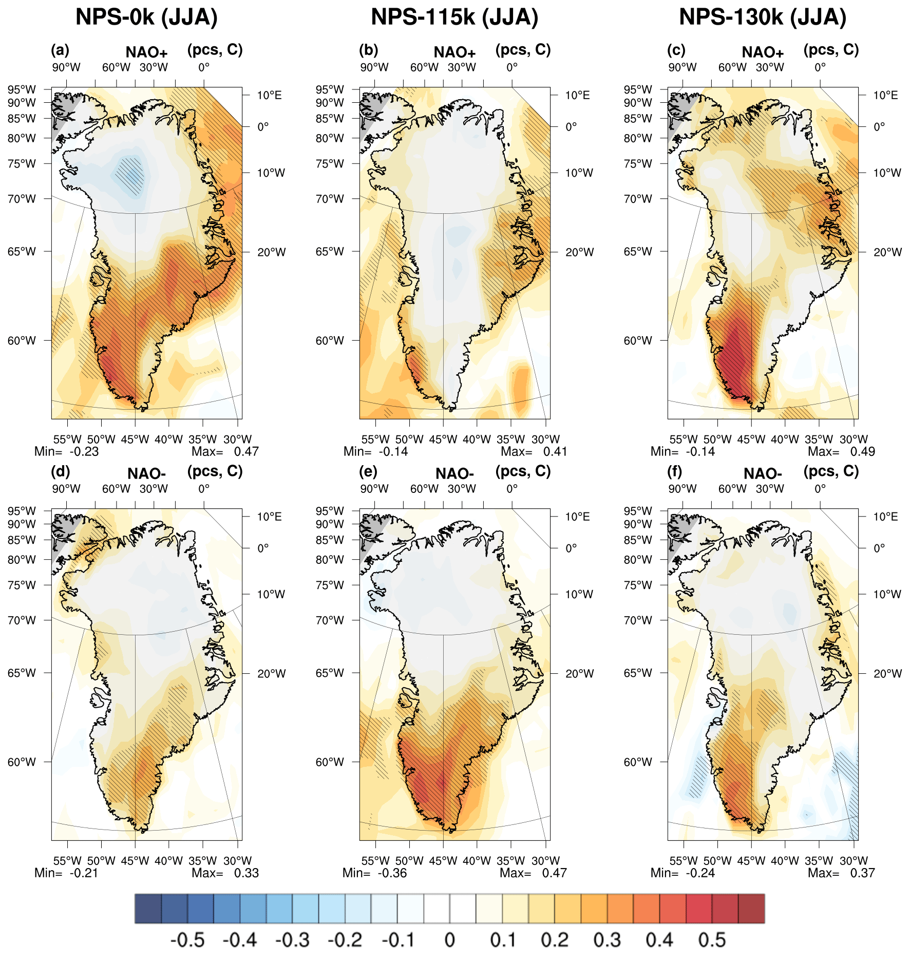
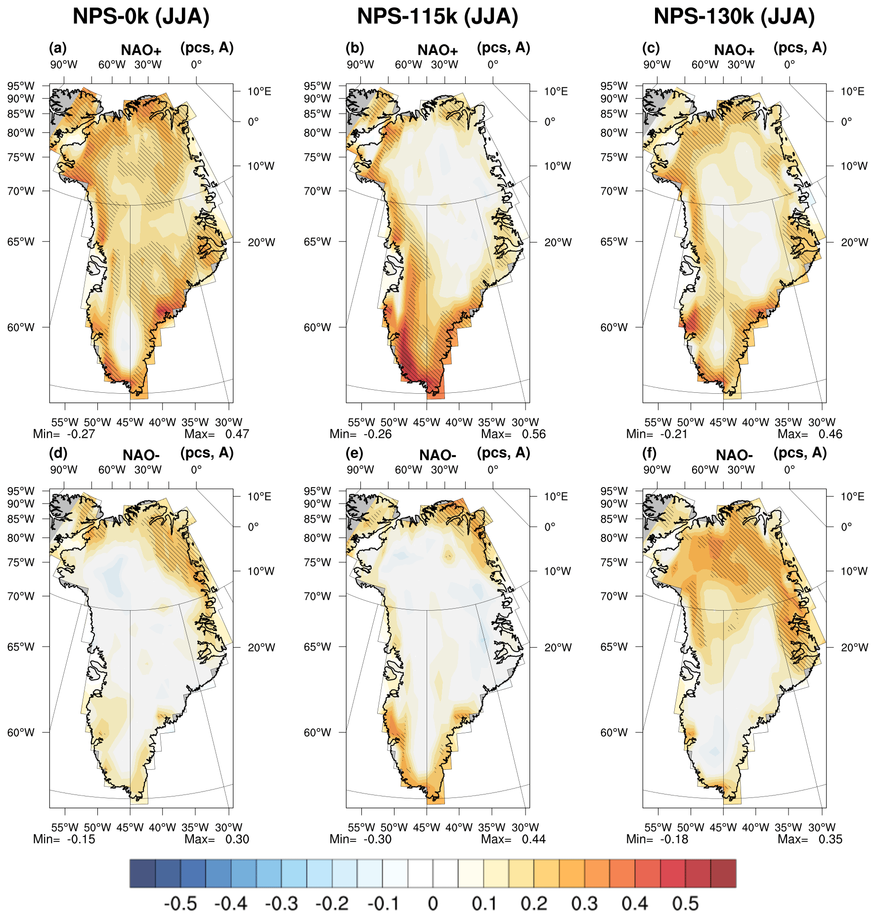
In order to go in to more detail in the analysis, we sampled positive and negative phases of the NAO and computed their grid-point correlation maps with accumulation in winter (Fig. 11) and summer (Fig. 12) and with melting in summer (Fig. 13). Situations with absolute values of the NAO index less than 1 standard deviation were excluded. The statistical significance of correlation coefficients is estimated at the 99 % confidence level.
In winter (Fig. 11), under all climates, the correlation of accumulation and both NAO phases is negative and significant on a band that stretches from northwestern to southeastern Greenland, approximately where the negative correlations between accumulation and the NAO index is strongest (Fig. 9a–c). Under situations with positive (negative) NAO index, the strongest negative correlations appear at 130 ka (the preindustrial period).
In summer (Fig. 12), the correlation between accumulation under positive or negative NAO phases exceeds 0.25 in most of south Greenland, except at 115 ka for positive NAO phases. The positive phase of the NAO favors accumulation in most of south Greenland in the preindustrial period (Fig. 12a) and 130 ka (Fig. 12c), i.e., under warm climates, whereas under the colder 115 ka climate, the negative phase of the NAO favors accumulation (Fig. 12e). The accumulated precipitation primarily arises from oceanic evaporation and atmospheric transport towards south Greenland. Oceanic evaporation is related to surface atmospheric forcing and sea surface temperature (SST) anomalies which can be generated by NAO phases. For example, the negative phase of the NAO is associated with negative SST anomalies from Baffin Bay to the Greenland Sea and positive SST anomalies in the central North Atlantic (Pinto and Raible, 2012, and references therein). Moreover, at 115 ka, the latitudinal insolation gradient (Fig. 6d) induces a larger northward atmospheric moisture transport from the warmer tropical ocean, supplying higher latitudes with moisture (Ramstein et al., 2005). Finally, central Greenland sees less precipitation, since moist air masses tend to generate precipitation and hence become drier on their way towards inland Greenland. In the northeastern part of the GrIS, significant correlations between accumulation and NAO are only seen at 130 ka for positive NAO phases. The correlation of melting with the positive phase of the NAO is greater than 0.25 mainly along the steepest margins of the GrIS except along the eastern coast north of 70∘ N for all climates (Fig. 13a–c). For the negative phase of the NAO, melting tends to be correlated with the NAO index only for 130 ka, along the eastern coast north of 70∘ N (Fig. 13d–f).
In this paper we examined the link between the NAO and the surface mass balance, accumulation and melting of the GrIS for the last interglacial and preindustrial climates. For this study we developed a configuration of CNRM-CM5.2 with enhanced atmospheric horizontal resolution on Greenland (40 to 55 km), which is reasonably suited to simulating the spatial variability in accumulation and surface melting. On the basis of a comparison with a regional simulation performed with MAR for 1980–1999, we showed that the simulated accumulation in our preindustrial simulation is realistic, whereas surface melting is greatly underestimated due to the minimum albedo (0.8) used in CNRM-CM5.2, which is too high.
The anomalies of the averaged SMB over the entire GrIS and the NAO index (normalized leading PC of detrended SLP anomalies) are weakly correlated in winter (around −0.2) and strongly correlated in summer (around 0.6) under all climates. These correlations are in broad agreement with those between SMB simulated by MAR and the NAO index computed from ERA-Interim for the period 1980–1999, which are −0.21 in winter and 0.40 in summer.
This study also emphasized the spatial pattern of the link between the NAO index with accumulation and melting. In winter, the spatial patterns of the correlations of accumulation with the NAO index are similar for all mean states, with negative (positive) correlations in the western (eastern) part of central Greenland. Both regions are characterized by relatively dry conditions, in contrast with south Greenland. Moreover, the similarity between regional patterns of winter accumulation and its correlation with the NAO index under all climates suggests a weak influence of the variability in insolation. In summer, the spatial patterns of accumulation and its correlation with the NAO index depend on the climate. The link between NAO and accumulation is all the stronger as the climate is warm (e.g., stronger at 130 ka than at 115 ka) and increases from the northwestern part of central Greenland towards the margins.
Compared with 115 ka, the melting is much stronger in northeast and east Greenland at 130 ka. This result suggests that in a warm climate, the altitude of the northern and northeastern parts of the GrIS could be much reduced. In south Greenland, the simulated patterns of melting under preindustrial and 115 ka climates are rather similar, with strong gradients confined to the margins associated with strong correlations with NAO. In north Greenland the preindustrial simulated melting can be viewed as intermediate between 115 and 130 ka patterns.
The last part of this work highlights the influence of both positive and negative phases of the NAO on accumulation and melting. In winter, under all climates, both NAO phases are negatively correlated to accumulation on a band that stretches from northwest to southeast Greenland. In summer, accumulation in south Greenland varies preferentially with the positive (negative) phase of the NAO in a warm (cold) climate. Under warm climates, the positive phase of the NAO favors the large-scale advection of moisture in southwest Greenland and subsequent precipitation. At 115 ka, the accumulation tends to be controlled by the negative phase of the NAO. The negative phase of the NAO is significantly correlated to melting only in northeast Greenland and all the more so as the climate is warm, whereas its positive phase promotes melting along the margins of the GrIS under all climates. By contrast, the positive phase of the NAO promotes melting along the margins of the GrIS under all climates but also inland in preindustrial climate. The link between melting and the negative NAO index does not appear on the margins of southern Greenland in a warm climate. The representation of the spatial structures of accumulation and melting and their links with NAO are both significantly improved due to the enhancement of horizontal resolution on Greenland in the NPS configuration compared with the CNRM-CM5 configuration used for CMIP5. Future work will investigate the contribution of sea ice and SST to the simulated links between SMB and its components with both phases of the NAO.
The data from NPS simulations are available from the authors upon request (silvana.buarque@meteo.fr).
The supplement related to this article is available online at: https://doi.org/10.5194/cp-14-1707-2018-supplement.
DSyM defined the scientific framework, verified numerical results, supervised the findings and improved the English of the paper. SRB conceived and performed the numerical simulations, developed the analytic calculations, performed the analysis and drafted the paper. Both authors provided discussed results, addressed critical feedback and shaped the analysis and the final version of the paper.
The authors declare that they have no conflict of interest.
The authors would like to thank Xavier Fettweis (University of Liège,
Belgium) for providing a regional simulation from MAR for the period
1979–2012. The authors would like to thank the referees, who
provided helpful comments that greatly improved the first version of the
paper. They are also grateful to Hugues Goosse, the editor, for evaluating
this article. The Silvana Ramos Buarque is grateful to Aurore
Voldoire for her help in handling the CNRM-CM model. Supercomputing resources
were provided by Météo-France/DSI, whom we thank for their support
and guidance. The figures were produced thanks to the NCAR Command Language
(NCL) Software (https://doi.org/10.5065/D6WD3XH5NCL) and the PCMDI Climate Data
Analysis Tools (CDAT), the use of which is hereby acknowledged.
Edited by: Hugues Goosse
Reviewed by: Xavier Fettweis and one anonymous referee
Ammann, C. M., Meehl, G. A., Washington, W. M., and Zender, C. S.: A monthly and latitudinally varying volcanic forcing dataset in simulations of 20th century climate: volcanic forcing dataset of 20th century, Geophys. Res. Lett., 30, 1657, https://doi.org/10.1029/2003GL016875, 2003.
Auger, J. D., Birkel, S. D., Maasch, K. A., Mayewski, P. A., and Schuenemann, K. C.: Examination of precipitation variability in southern Greenland: Southern Greenland Precipitation, J. Geophys. Res.-Atmos., 122, 6202–6216, https://doi.org/10.1002/2016JD026377, 2017.
Berger, A. L.: Long-Term Variations of Caloric Insolation Resulting from the Earth's Orbital Elements, Quaternary Res., 9, 139–167, https://doi.org/10.1016/0033-5894(78)90064-9, 1978.
Berger, A.: Milankovitch Theory and climate, Rev. Geophys., 26, 624–657, https://doi.org/10.1029/RG026i004p00624, 1988.
Björnsson, H. and Venegas, S. A.: A manual for EOF and SVD analyses of climatic data, CCGCR Report, 97, 112–134, 1997.
Born, A. and Nisancioglu, K. H.: Melting of Northern Greenland during the last interglaciation, The Cryosphere, 6, 1239–1250, https://doi.org/10.5194/tc-6-1239-2012, 2012.
Bromwich, D. H., Chen, Q., Li, Y., and Cullather, R. I.: Precipitation over Greenland and its relation to the North Atlantic Oscillation, J. Geophys. Res.-Atmos., 104, 22103–22115, https://doi.org/10.1029/1999JD900373, 1999.
Chauvin, F., Royer, J.-F., and Déqué, M.: Response of hurricane-type vortices to global warming as simulated by ARPEGE-Climat at high resolution, Clim. Dynam., 27, 377–399, https://doi.org/10.1007/s00382-006-0135-7, 2006.
Courtier, P. and Geleyn, J.-F.: A global numerical weather prediction model with variable resolution: Application to the shallow-water equations, Q. J. Roy. Meteor. Soc., 114, 1321–1346, https://doi.org/10.1002/qj.49711448309, 1988.
Dahl-Jensen, D., Albert, M. R., Aldahan, A., Azuma, N., Balslev-Clausen, D., Baumgartner, M., Berggren, A.-M., Bigler, M., Binder, T., and Blunier, T.: Eemian interglacial reconstructed from a Greenland folded ice core, Nature, 493, 489–494, https://doi.org/10.1038/nature11789, 2013.
Dee, D. P., Uppala, S. M., Simmons, A. J., Berrisford, P., Poli, P., Kobayashi, S., Andrae, U., Balmaseda, M. A., Balsamo, G., Bauer, P., Bechtold, P., Beljaars, A. C. M., van de Berg L., Bidlot, J., Bormann, N., Delsol, C., Dragani, R., Fuentes, M., Geer, A. J., Haimberger, L., Healy, S. B., Hersbach, H., Holm, E. V., Isaksen, L., Kallberg, P., Köhler, M., Matricardi, M., McNally, A. P., Monge-Sanz, B. M., Morcrette, J.-J., Park, B.-K., Peubey, C., de Rosnay, P., Tavolato, C., Thepaut J.-N., and Vitart, F.: The ERA-Interim reanalysis: configuration and performance of the data assimilation system, Q. J. Roy. Meteor. Soc., 137, 553–597, https://doi.org/10.1002/qj.828, 2011.
Déqué, M., Dreveton, C., Braun, A., and Cariolle, D.: The ARPEGE/IFS atmosphere model: a contribution to the French community climate modelling, Clim. Dynam., 10, 249–266, 1994.
Doblas-Reyes, F. J., Casado, M. J., and Pastor, M. A.: Sensitivity of the Northern Hemisphere blocking frequency to the detection index, J. Geophys. Res.-Atmos., 107, 1–22, https://doi.org/10.1029/2000JD000290, 2002.
Douville, H., Royer, J.-F., and Mahfouf, J.-F.: A new snow parameterization for the Meteo-France climate model, Clim. Dynam., 12, 21–35, https://doi.org/10.1007/BF00208760, 1995.
Ettema, J., van den Broeke, M. R., van Meijgaard, E., van de Berg, W. J., Bamber, J. L., Box, J. E., and Bales, R. C.: Higher surface mass balance of the Greenland ice sheet revealed by high-resolution climate modeling, Geophys. Res. Lett., 36, L12501, https://doi.org/10.1029/2009GL038110, 2009.
Fettweis, X., Belleflamme, A., Erpicum, M., Franco, B., and Nicolay, S.: Estimation of the sea level rise by 2100 resulting from changes in the surface mass balance of the Greenland ice sheet, in: Climate Change-Geophysical Foundations and Ecological Effects, InTech., 503-520, https://doi.org/10.5772/23913, 2011.
Fettweis, X., Hanna, E., Lang, C., Belleflamme, A., Erpicum, M., and Gallée, H.: Brief communication “Important role of the mid-tropospheric atmospheric circulation in the recent surface melt increase over the Greenland ice sheet”, The Cryosphere, 7, 241–248, https://doi.org/10.5194/tc-7-241-2013, 2013a.
Fettweis, X., Franco, B., Tedesco, M., van Angelen, J. H., Lenaerts, J. T. M., van den Broeke, M. R., and Gallée, H.: Estimating the Greenland ice sheet surface mass balance contribution to future sea level rise using the regional atmospheric climate model MAR, The Cryosphere, 7, 469–489, https://doi.org/10.5194/tc-7-469-2013, 2013b.
Folland, C. K., Knight, J., Linderholm, H. W., Fereday, D., Ineson, S., and Hurrell, J. W.: The summer North Atlantic Oscillation: past, present, and future, J. Climate, 22, 1082–1103, https://doi.org/10.1175/2008JCLI2459.1, 2009.
Fürst, J. J., Goelzer, H., and Huybrechts, P.: Ice-dynamic projections of the Greenland ice sheet in response to atmospheric and oceanic warming, The Cryosphere, 9, 1039–1062, https://doi.org/10.5194/tc-9-1039-2015, 2015.
Gallée, H. and Duynkerke, P. G.: Air-snow interactions and the surface energy and mass balance over the melting zone of west Greenland during the Greenland Ice Margin Experiment, J. Geophys. Res.-Atmos., 102, 13813–13824, 1997.
Geoffroy, O., Saint-Martin, D., Voldoire, A., Salas y Mélia, D., and Sénési, S.: Adjusted radiative forcing and global radiative feedbacks in CNRM-CM5, a closure of the partial decomposition, Clim. Dynam., 42, 1807–1818, https://doi.org/10.1007/s00382-013-1741-9, 2014.
Gillet-Chaulet, F., Gagliardini, O., Seddik, H., Nodet, M., Durand, G., Ritz, C., Zwinger, T., Greve, R., and Vaughan, D. G.: Greenland ice sheet contribution to sea-level rise from a new-generation ice-sheet model, The Cryosphere, 6, 1561–1576, https://doi.org/10.5194/tc-6-1561-2012, 2012.
Giordani, H., Caniaux, G., and Voldoire, A.: Intraseasonal mixed-layer heat budget in the equatorial Atlantic during the cold tongue development in 2006, J. Geophys. Res.-Ocean., 118, 650–671, https://doi.org/10.1029/2012JC008280, 2013.
Hanna, E., Jones, J. M., Cappelen, J., Mernild, S. H., Wood, L., Steffen, K., and Huybrechts, P.: The influence of North Atlantic atmospheric and oceanic forcing effects on 1900–2010 Greenland summer climate and ice melt/runoff, Int. J. Climatol., 33, 862–880, https://doi.org/10.1002/joc.3475, 2013a.
Hanna, E., Fettweis, X., Mernild, S. H., Cappelen, J., Ribergaard, M. H., Shuman, C. A., Steffen, K., Wood, L., and Mote, T. L.: Atmospheric and oceanic climate forcing of the exceptional Greenland ice sheet surface melt in summer 2012, Int. J. Climatol., 34, 1022–1037, https://doi.org/10.1002/joc.3743, 2013b.
Hanna, E., Cropper, T. E., Jones, P. D., Scaife, A. A., and Allan, R.: Recent seasonal asymmetric changes in the NAO (a marked summer decline and increased winter variability) and associated changes in the AO and Greenland Blocking Index, Int. J. Climatol., 35, 2540–2554, https://doi.org/10.1002/joc.4157, 2015.
Hewitt, H. T., Copsey, D., Culverwell, I. D., Harris, C. M., Hill, R. S. R., Keen, A. B., McLaren, A. J., and Hunke, E. C.: Design and implementation of the infrastructure of HadGEM3: The next-generation Met Office climate modelling system, Geosci. Model Dev., 4, 223–253, https://doi.org/10.5194/gmd-4-223-2011, 2011.
Hortal, M. and Simmons, A. J.: Use of reduced Gaussian grids in spectral models, Mon. Weather Rev., 119, 1057–1074, 1991.
Hurrell, J. W.: Decadal trends in the North Atlantic Oscillation: regional temperatures and precipitation, Science-AAAS-Weekly Paper Edition, 269, 676–678, https://doi.org/10.1126/science.269.5224.676, 1995.
Le Moigne, P., Boone, A., Calvet, J. C., Decharme, B., Faroux, S., Gibelin, A. L., Lebeaupin, C., Mahfouf, J. F., Martin, E., and Masson, V.: SURFEX scientific documentation, Note de centre (CNRM/GMME), Météo-France, Toulouse, France, 2009.
Lenaerts, J. T. M., Van Den Broeke, M. R., Scarchilli, C., and Agosta, C.: Impact of model resolution on simulated wind, drifting snow and surface mass balance in Terre Adélie, East Antarctica, J. Glaciol., 58, 821–829, https://doi.org/10.3189/2012JoG12J020, 2012.
Lorant, V. and Royer, J.-F.: Sensitivity of equatorial convection to horizontal resolution in aquaplanet simulations with a variable-resolution GCM, Mon. Weather Rev., 129, 2730–2745, https://doi.org/10.1175/1520-0493, 2001.
Madec, G.: the NEMO team: NEMO ocean engine, version 3.6 stable, Technical Note of the Institut Pierre-Simon Laplace (IPSL) No. 27, ISSN No. 1288-1619, 2015.
Nghiem, S. V., Hall, D. K., Mote, T. L., Tedesco, M., Albert, M. R., Keegan, K., Shuman, C. A., DiGirolamo, N. E., and Neumann, G.: The extreme melt across the Greenland ice sheet in 2012, Geophys. Res. Lett., 39, 1–6, https://doi.org/10.1029/2012GL053611, 2012.
Oki, T. and Sud, Y. C.: Design of Total Runoff Integrating Pathways (TRIP) – A global river channel network, Earth Interact., 2, 1–37, https://doi.org/10.1175/1087-3562(1998)002, 1998.
Pinto, J. G. and Raible, C. C.: Past and recent changes in the North Atlantic oscillation, WIRES Clim. Change, 3, 79–90, https://doi.org/10.1002/wcc.150, 2012.
Pithan, F. and Mauritsen, T.: Arctic amplification dominated by temperature feedbacks in contemporary climate models, Nat. Geosci., 7, 181–184, https://doi.org/10.1038/ngeo2071, 2014.
Ramstein, G., Khodri, M., Donnadieu, Y., Fluteau, F., and Goddéris, Y.: Impact of the hydrological cycle on past climate changes: three illustrations at different time scales, C. R. Geosci., 337, 125–137, https://doi.org/10.1016/j.crte.2004.10.016, 2005.
Salas y Mélia, D. : A global coupled sea ice-ocean model, Ocean Model., 4, 137–172, https://doi.org/10.1016/S1463-5003(01)00015-4, 2002.
Sasgen, I., van den Broeke, M., Bamber, J. L., Rignot, E., Sørensen, L. S., Wouters, B., Martinec, Z., Velicogna, I., and Simonsen, S. B.: Timing and origin of recent regional ice-mass loss in Greenland, Earth Planet. Sc. Lett., 333, 293–303, https://doi.org/10.1016/j.epsl.2012.03.033, 2012.
Szopa, S., Balkanski, Y., Schulz, M., Bekki, S., Cugnet, D., Fortems-Cheiney, A., Turquety, S., Cozic, A., Déandreis, C., and Hauglustaine, D.: Aerosol and ozone changes as forcing for climate evolution between 1850 and 2100, Clim. Dynam., 40, 2223–2250, https://doi.org/10.1007/s00382-012-1408-y, 2013.
Valcke, S., Budich, R. G., Carter, M., Guilyardi, E., Foujols, M.-A., Lautenschlager, M., Redler, R., Steenman-Clark, L., and Wedi, N.: The PRISM software framework and the OASIS coupler, in: The Australian Community Climate Earth System Simulator (ACCESS) – Challanges and Opportunities, edited by: Hollies, A. J. and Kariko, A. P., BMRC Research Report, 132–140, Bur. Met. Australia, 2006.
Vernon, C. L., Bamber, J. L., Box, J. E., Van den Broeke, M. R., Fettweis, X., Hanna, E., and Huybrechts, P.: Surface mass balance model intercomparison for the Greenland ice sheet, The Cryosphere, 7, 599–614, https://doi.org/10.5194/tc-7-599-2013, 2013.
Voldoire, A., Sanchez-Gomez, E., y Mélia, D. S., Decharme, B., Cassou, C., Sénési, S., Valcke, S., Beau, I., Alias, A., and Chevallier, M.: The CNRM-CM5. 1 global climate model: description and basic evaluation, Clim. Dynam., 40, 2091–2121, https://doi.org/10.1007/s00382-011-1259-y, 2013.
Yan, Q., Wang, H., Johannessen, O. M., and Zhang, Z.: Greenland ice sheet contribution to future global sea level rise based on CMIP5 models, Adv. Atmos. Sci., 31, 8–16, https://doi.org/10.1007/s00376-013-3002-6, 2014.
- Abstract
- Introduction
- Features of the climate modeling simulations
- Evaluation of the preindustrial control integration
- Greenland climate, NAO and GrIS SMB during the 130 ka, 115 ka and preindustrial periods
- Conclusions and perspectives
- Data availability
- Author contributions
- Competing interests
- Acknowledgements
- References
- Supplement