the Creative Commons Attribution 4.0 License.
the Creative Commons Attribution 4.0 License.
 | 01 Nov 2018
Influence of radiative forcing factors on ground–air temperature coupling during the last millennium: implications for borehole climatology
J. Fidel González-Rouco
Elena García-Bustamante
Jorge Navarro-Montesinos
Norman Steinert
Past climate variations may be uncovered via reconstruction methods that use proxy data as predictors. Among them, borehole reconstruction is a well-established technique to recover the long-term past surface air temperature (SAT) evolution. It is based on the assumption that SAT changes are strongly coupled to ground surface temperature (GST) changes and transferred to the subsurface by thermal conduction. We evaluate the SAT–GST coupling during the last millennium (LM) using simulations from the Community Earth System Model LM Ensemble (CESM-LME). The validity of such a premise is explored by analyzing the structure of the SAT–GST covariance during the LM and also by investigating the evolution of the long-term SAT–GST relationship. The multiple and single-forcing simulations in the CESM-LME are used to analyze the SAT–GST relationship within different regions and spatial scales and to derive the influence of the different forcing factors on producing feedback mechanisms that alter the energy balance at the surface. The results indicate that SAT–GST coupling is strong at global and above multi-decadal timescales in CESM-LME, although a relatively small variation in the long-term SAT–GST relationship is also represented. However, at a global scale such variation does not significantly impact the SAT–GST coupling, at local to regional scales this relationship experiences considerable long-term changes mostly after the end of the 19th century. Land use land cover changes are the main driver for locally and regionally decoupling SAT and GST, as they modify the land surface properties such as albedo, surface roughness and hydrology, which in turn modifies the energy fluxes at the surface. Snow cover feedbacks due to the influence of other external forcing are also important for corrupting the long-term SAT–GST coupling. Our findings suggest that such local and regional SAT–GST decoupling processes may represent a source of bias for SAT reconstructions from borehole measurement, since the thermal signature imprinted in the subsurface over the affected regions is not fully representative of the long-term SAT variations.
- Article
(15004 KB) - Full-text XML
- BibTeX
- EndNote


Improving our knowledge of the last millennium (LM) climate variability is key for a better understanding of the mechanisms that determine the Earth system response to natural (solar, volcanic and orbital) and anthropogenic (land use and atmospheric composition changes) external forcings (Masson-Delmotte et al., 2013). Instrumental records represent the most adequate alternative to study past climate variations. However, they only provide coverage since the mid-19th century (Hansen et al., 2010; Jones et al., 2012). Therefore, to understand the nature of climate variability operating on longer temporal scales, LM reconstructions from a variety of proxy data (Jones et al., 2009) and simulations using general climate models (GCMs) are generally employed.
The current available LM temperature reconstructions agree, depicting a general pattern of temperature evolution going from a relatively warmer period at the beginning of the LM (MCA; Medieval Climate Anomaly) to a colder period from about 1450 to ca. 1850 (LIA; Little Ice Age), which is interrupted by the industrial warming in the 19th century (Masson-Delmotte et al., 2013). Despite this general agreement, there is still a large range of uncertainty that stems from different sources, including different reconstruction methods, various calibration and verification processes, spatial and temporal coverage, the different proxy locations (land, land and ocean, etc.) and the alternative statistical methods employed (Fernández-Donado et al., 2013; Jones et al., 2009). For instance, the range of uncertainty during the MCA regarding reconstructing Northern Hemisphere (NH) temperature is about 0.6 ∘C. Furthermore, Ammann and Wahl (2007) estimate that the cooling during the Maunder Minimum (1645–1745) relative to present is about 0.7 ∘C, while Christiansen and Ljungqvist (2012) report a colder LIA (1.4 ∘C) which is similar to findings by Pollack and Smerdon (2004).
Addressing the range of uncertainties in reconstructing past temperature changes is relevant not only for assessing our understanding of past temperature changes and the confidence we have on available estimates (Masson-Delmotte et al., 2013), but also for model–data comparison exercises (Fernández-Donado et al., 2013) and for constraining the range of estimates of the system response to changes in the external forcing, i.e., the sensitivity of the climate system (Fernández-Donado et al., 2013; Hegerl et al., 2006).
Borehole temperature inversion is a well-established reconstruction technique and leans on two main assumptions: first, surface air temperatures (SAT) are expected to be closely coupled to ground surface temperatures (GST); second, variations in SAT propagate downward through the subsurface via conduction (Pollack et al., 1998; Smerdon et al., 2003, 2004). As a result, a thermal signature of the surface temperature is imprinted in the subsurface. This reconstruction technique is limited to recovering only the low-frequency information (decadal, and longer timescales) since the soil acts as a low-pass filter and progressively filters out the higher-frequency variations with depth. Oscillations with periods on the order of days only penetrate ∼50 cm deep (Smerdon and Stieglitz, 2006), seasonal cycles are solely observed close to the surface (<10 m depth), decadal variations propagate within the upper 50 m and multi-centennial changes within the LM are observed in the upper 500 m below the surface (Mareschal and Beltrami, 1992; Pollack and Huang, 2000).
As with every type of reconstruction method, the borehole technique is also subject to diverse sources of uncertainty. One of them is that the assumption of a conductive heat transfer may not always be substantiated, as non-conductive processes such as advection and convection may influence or even dominate the subsurface thermal regime (Kukkonen and Clauser, 1994) in areas with important groundwater flows or geothermal activity. Nevertheless, a number of studies suggest that the impacts of such processes can be reduced with the appropriate treatment of the affected borehole temperature logs (Bodri and Cermak, 2005; Ferguson et al., 2006; Kohl, 1998)
Additionally, the most important contributions to uncertainty arise from changes in surface processes that affect the SAT–GST coupling. Snow cover is especially important since it insulates the ground surface from the cold winter air causing large differences between the soil and air temperatures (Bartlett et al., 2004; Beltrami and Kellman, 2003; Pollack and Huang, 2000; Stieglitz et al., 2003). The impact of this effect on borehole theory has caused considerable discussion. Mann and Schmidt (2003) argued that borehole-based reconstructions may be substantially biased by this seasonal influence of snow cover. Hence, under changing snow cover conditions GST may be not completely representative of SAT variations. Chapman et al. (2004) argued against this based on the assumption that SAT and GST coupling is strong at longer than seasonal timescales; therefore, snow biases would only influence the high-frequency oscillations. Additionally, the long-term SAT–GST coupling has also been supported by observations (Smerdon et al., 2003, 2004) and modeling assessments (Bartlett et al., 2005; González-Rouco et al., 2003, 2006, 2009). Besides snow cover, other land surface and soil properties such as soil water content, vegetation and land use land cover (LULC) changes also have the potential to impact SAT–GST coupling. For instance, deforestation, afforestation and other land cover changes modify the land-surface properties including albedo, roughness and evapotranspiration altering the energy transfer between the atmosphere and the ground (Anderson et al., 2011). In a recent study, MacDougall and Beltrami (2017) found that deforestation tends to warm the ground surface mainly by reducing the transport of heat away from the surface. They also found that such continuous vegetation changes would result in long-term surface temperature anomalies; thus, deforestation should be considered as a possible source of bias for temperature reconstructions from subsurface temperatures.
One way of addressing the uncertainties of paleoclimate reconstruction methods is by using climate model simulations as a surrogate reality in which pseudoproxy records of varying complexity are created and reconstruction methods are replicated in pseudoproxy experiments (PPEs) mimicking real-world cases (Smerdon, 2012). The robustness of using the borehole method for reconstructing past SAT variations has been tested in PPEs (Beltrami et al., 2006; González-Rouco et al., 2003, 2006, 2009). González-Rouco et al. (2003) investigated the relationship between simulated SAT and GST from interannual to centennial timescales in a forced climate simulation of the LM (1000–1900 common era; CE) using the ECHO-G GCM (Legutke and Voss, 1999). They found that in spite of the seasonal and longer-term variability of snow cover, the coupling was stable for decadal and longer timescales, meaning that GST should be a good proxy for long-term SAT variations. González-Rouco et al. (2006) extended this analysis by implementing the borehole method in the simplified reality of the same model. They simulated underground temperature perturbation profiles using a heat-conduction forward model driven by simulated GST. Then, they applied an inversion approach to reconstruct ground surface temperature histories from the simulated profiles. Their results supported the overall performance of the borehole methodology.
García-García et al. (2016) employed a similar approach to González-Rouco et al. (2006) in order to retrieve past GST variations from GCMs: both studies applied an inversion method. They simulated global synthetic temperature profiles using a one-dimensional conductive model driven by simulated GST as an upper boundary condition from the CMIP5/PMIP3 (Taylor et al., 2012) LM simulations. Unlike the GCMs used in the early works that do not incorporate some external forcings, the PMIP3/CMIP5 simulations include a larger representation of LM forcings than pre-PMIP3 experiments (Fernández-Donado et al., 2013; Taylor et al., 2012) incorporating a variety of land-surface model components. Their results have reinforced the reliability of recovering past global surface temperature variations from subsurface temperature measurements using current state-of-the-art GCMs.
The previous analyses support estimations of global/hemispheric past temperature obtained from borehole temperature inversions. First, they support the overall performance of the methodology in retrieving past GST histories from borehole profiles. Second, the use of up-to-date forcing representations in CMIP5 model ensembles also ensures that long-term alterations of surface properties like those induced by LULC changes, the effect of anthropogenic aerosols cooling and the potential long-term snow cover feedbacks induced by both forcings, do not seem to bias inversion results at global/hemispheric scales. In spite of these positive results, the analysis of last generation model experiments, including the complete set of agreed CMIP5 forcings (Schmidt et al., 2011, 2012) in the so-called “all-forcing” experiments, does not allow for insights into the individual effect of each of the forcings and the related feedbacks, at either global/hemispherical or continental/regional scales. This would be desirable in order to quantify the effect of the individual forcings on SAT–GST coupling and to obtain estimates of its particular temporal evolution which would allow for the disentanglement of its contribution from that of other forcings. Therefore, the present work considers all-forcing and single-forcing types of experiments in order to address how state-of-the-art climate models simulate SAT–GST coupling from global to regional scales and to evaluate the potential influence of the external forcings on the SAT–GST relationship. This will also provide information about where and when a decoupling of SAT–GST may exist, with implications for borehole inversion practices at different spatiotemporal scales. For this purpose, we use the Community Earth System Model–Last Millennium Ensemble (Otto-Bliesner et al., 2016), which is the largest existing ensemble of LM simulations with a single model to date and has not been used in previous assessments of this kind. The CESM-LME includes all- and single-forcing experiments that jointly or separately consider the transient evolution of solar variability, volcanic activity, orbital changes, greenhouse gases (GHGs), anthropogenic aerosols and LULC (see details in Sect. 2)
Using all-forcing simulations (ALL-F hereafter) allows for the evaluation of the SAT–GST relationship throughout the LM with a realistic representation of real-world conditions. Additionally, the single-forcing experiments are suitable for identifying the specific role that each forcing might play and its “fingerprint” (Hegerl et al., 2011) on the presence of biases in the SAT–GST coupling. Most external natural (solar and volcanic variability) and anthropogenic (GHGs, LULC and aerosols) forcings have the potential to indirectly affect SAT–GST thermodynamics through snow cover feedbacks (Hartmann et al., 2013). Moreover, LULC changes can also have a direct influence on SAT–GST. Over the LM the Earth′s land cover has been substantially modified by the replacement of natural ecosystems with agricultural land, especially since the industrial period (Hurtt et al., 2009; Pongratz et al., 2008). Such land use changes have the potential to alter the surface energy balance by modifying energy fluxes and moisture budgets (Anderson et al., 2011; Betts, 2001; Betts et al., 2007; Brovkin et al., 2006; Zhao and Jackson, 2014) leading to direct impacts on the atmosphere and ground–surface temperature relationship (MacDougall and Beltrami, 2017). Furthermore, vegetation changes may additionally lead to indirect non-linear effects that are relevant in the borehole context. The most important of these is the fact that deforestation at high latitudes leads to an increase in snow cover; this is due to the fact that low vegetation accumulates continuous snow cover more readily than forests in early winter favoring its permanence longer in spring (Myhre et al., 2013). The local-, regional- and large-scale implications of these interactions on long-term climate variability and specifically on the validity of the borehole method assumptions have not been explored so far.
The first part of this paper (Sect. 2) describes the CESM-LME simulations and forcings used in the experiment. Subsequently, Sect. 3 describes the methodological approach employed for the analysis of the coupling between SAT and GST during the LM. Section 4 presents the main results in the analysis of the global covariance of SAT, GST and soil temperature (ST) at different model depths throughout the LM. This analysis includes the global SAT–GST long-term coupling at annual and seasonal timescales. The latter helps identify the impacts of seasonality on the SAT–GST coupling. In addition, the spatial distribution of the covariance structure, as well as the SAT–GST offset, are illustrated. This allows for the detection of possible failures in the air–ground temperature coupling at regional and local scales. The spatial analysis is extended to investigate the heat transfer within the shallow subsurface by comparing GST relative to deep model layers. Section 4.1 specifically addresses the long-term trend of the SAT–GST relationship in order to evaluate whether this association experiences variation with time during the simulated LM. Finally, Sect. 5 provides a discussion about the implications of decoupling processes at different temporal and spatial scales for the borehole temperature reconstruction method.
This analysis considers LM simulations produced with version 1.1 of CESM (Hurrell et al., 2013). The Community Atmosphere Model version 5 (Neale et al., 2012) is used as the atmospheric component, the Parallel Ocean Program version 2 (Smith et al., 2010) represents the ocean component, including the Los Alamos sea ice model (Hunke et al., 2015). The horizontal resolution of the CESM-LME is ∼2∘ over the atmosphere and land and ∼1∘ in the ocean and sea ice (Otto-Bliesner et al., 2016).
Table 1Soil layers and node depths in the CLM4. Note that the node depths, which are the depths at which the thermal properties are defined for soil layers (Oleson et al., 2010), do not necessarily coincide with the center of the layer depth.
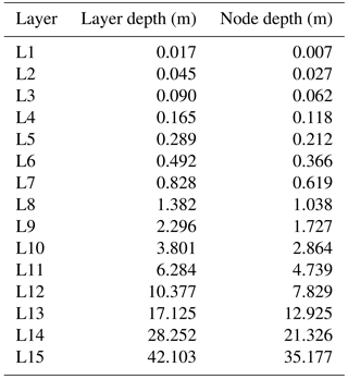
The land surface component in the CESM1 is the Community Land Model version 4 (Lawrence et al., 2011) which incorporates some improvements relative to the previous version (Oleson et al., 2008) regarding the representation of land surface processes that are important for the energy transfer between the atmosphere and the soil (Oleson et al., 2010). Some of these include a better description of ground evaporation, thermal and hydrologic properties of organic soil, the ground depth, snow albedo, snow cover fraction and burial fraction of vegetation by snow (Lawrence et al., 2011). In addition, The CLM4 has the deepest bottom boundary condition placement (BBCP) among the current land surface models to date, placed at a depth of 42.1 m, discretized into 15 layers (see Table 1) and including up to 5 additional layers in the overlying snowpack. This is relevant for borehole reconstruction applications because previous studies have shown that shallow bottom boundary conditions may not reliably represent the downward propagation of the temperature signal corrupting the amplitude attenuation and the phase shift (Alexeev et al., 2007; Nicolsky et al., 2007; Smerdon and Stieglitz, 2006), particularly for trends at timescales longer than decadal, from the comparison of energy storage in model simulations and borehole profiles (MacDougall et al., 2010). Therefore, this improved and deeper land surface model allows for the analysis of the coupling between SAT and GST in a more realistic atmosphere–subsurface heat transfer scheme.
Vieira et al. (2011)Gao et al. (2008)MacFarling Meure et al. (2006)Pongratz et al. (2008)Hurtt et al. (2009)Berger et al. (1993)Table 2Simulations and LM external forcing reconstructions used in CESM-LME. The single-forcing simulations cover from 850 to 2005 CE except for those of anthropogenic ozone and aerosols that span the period from 1850 to 2005 CE. The legend for external forcing is as follows: SOL represents changes in total solar irradiance; VOLC represents volcanic activity; GHG represents concentrations of the well-mixed greenhouse gases CO2, CH2 and N2O; LULC represents land use land cover changes; ORB represents orbital variations; and OZ/AER represents anthropogenic ozone and aerosols.
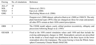
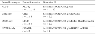
The CESM-LME incorporates ALL-F simulations with natural and anthropogenic forcings that were chosen following those used in Landrum et al. (2012). The model is composed of a total of 30 simulations including a subset of 10 simulations that incorporate all of the LM external forcings and smaller subsets of single-forcing simulations that consider each forcing individually (see Table 2 for details and references therein). The simulations used in this study and how they trace back to the original experiment names produced by Otto-Bliesner et al. (2016) are shown in Table 3.
Table 3Simulations used in this study are from the CESM-LME. The first and second columns present the acronyms used in this paper for ensembles and ensemble members, respectively. The ID of the original experiment files is provided in column 3.
In the present work the LM refers to the period from 850 to 2005 CE while the periods from 850 to 1850 CE and 1851 to 2005 CE refer to preindustrial and industrial, respectively. The 2 m air temperature is used for SAT, and the first land model level (Table 1) represents GST. Additionally, the ST at different depths, denoted by the subscript notation STL2, STL3, …, STL15, is used to address different aspects of the subsurface heat transport within the CESM-LME. The simulated ST does not include data over the Antarctic region; therefore, this region is excluded from the analysis.
The relationship between SAT and GST is analyzed from two complementary perspectives. First, the covariance during the LM of the global SAT and GST anomalies relative to the 1851–2005 CE period is assessed at an interannual scale. Similarly, the spatial patterns of the correlation between SAT and GST are also analyzed. This spatial analysis is extended to the differences between the SAT and GST LM mean values, as this gives an additional measure of the energy exchange across the air–ground interface (Bartlett et al., 2004) that may help characterize a potential air–ground temperature decoupling. In addition, the same spatial analysis is carried out for the differences between GST and STL8 in order to gain insight into processes affecting the pure conductive subsurface transport assumption within the shallow subsurface. For specific cases where SAT and GST exhibit some kind of decoupling, a description of the main processes that lead to this decoupling at local and regional scales is presented. For this purpose, the evolution of SAT, GST and ST at different depths is assessed over the last 105 years of the simulation period (1900–2005 CE) for the cases of interest. In some particular examples, additional variables (e.g., latent and sensible heat fluxes or snow cover) are also included for a better description of the physical processes. The purpose of such analyses is to provide some examples rather than detailing the minutiae of the processes that lead to different SAT–GST responses at many different locations. For the analysis described above the ALL-F ensemble will be used. This provides a more complete and realistic representation of real world conditions than the single forcing runs, from the point of view of the forcings considered. It also allows for the use of the surrogate reality of the CEMS-LME model as a test bed for detecting potential sources of deviations in the SAT–GST relationship during the LM.

Figure 1(a) Annual, (c) DJF and (e) JJA global LM evolution of SAT, GST, STL8 and STL15 anomalies relative to the 1850–2005 CE period for the ALL-F2 ensemble member. (b) Annual, (d) DJF and (f) JJA global LM evolution of the SAT–GST offset (SAT minus GST anomalies) and the global percentage of snow cover. Dashed lines are the result of a two-phase regression, indicating the linear trend that represents the best fit to the data before and after the estimated point of change. For snow cover, dashed lines represent linear fits to the data using the change points found for SAT–GST. All series are 31-year moving average filter outputs except for STL15, which is represented as the direct model output.
We then focus on the assessment of the long-term trend in the SAT–GST relationship. Non-stationarity in such an association at long timescales (multi-decadal to multi-centennial) might imply that GST variations would not be representative of the SAT variations; therefore, this would result in unreliable inferences of past climate change (Bartlett et al., 2004). A two-phase regression model (Solow, 1987) is applied to address this issue, which allows for the detection of changes in the long-term trend of the SAT–GST relationship without imposing any a priori temporal condition on their occurrence. The year of change is identified, as well as the trend before and after the change. The timing of change and the magnitude of trends are suggestive of long-term changes in the surface coupling. Initially, this assessment is performed at a global scale by analyzing the LM evolution of global SAT minus GST anomalies. The analysis of the long-term trend is then extended starting from the independent evaluation of SAT and GST linear trends during the industrial period, as the largest changes are expected to occur within this period. In this section of the study, besides the ALL-F ensemble, we also considered the GHG-only, LULC-only and OZ/AER-only ensembles because they have the highest potential for altering the land surface characteristics. This allows for the identification of the influence of each forcing on the LM SAT–GST coupling, including changes in snow cover, soil moisture, and latent and sensible heat variations. The linear trend analysis of SAT and GST gives a general view of their evolution through industrial times and a first glance at the most important areas where long-term SAT–GST decoupling may exist in response to changes in external forcings and related feedbacks. Although these types of processes have mostly taken place during industrial times, GHGs and land use also experienced notable changes before 1850 CE (Otto-Bliesner et al., 2016; Pongratz et al., 2008; Ramankutty and Foley, 1992). The application of the two-phase regression to the complete LM permits for the identification of changes that occurred before 1850 CE.
Table 4Temporal correlation coefficients between last millennium SAT–GST, SAT–STL8 and SAT–STL15 anomalies relative to the 1850–2005 mean for the experiment shown in Fig. 1. The left side indicates the correlation at a yearly resolution, whereas the right side shows 31-year low-pass filter outputs of SAT, GST, STL8 and STL15 for the annual, DJF and JJA time periods. Coefficients highlighted in bold are statistically significant at p<0.05.
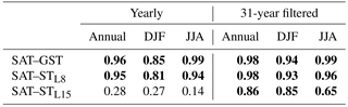
CESM-LME supports the assumption that SAT is tightly coupled with GST at global scales and longer than multi-decadal scales. Figure 1a illustrates the stability of the coupling at global scales during the LM using the ALL-F2 ensemble member as an example. Results are comparable for other ALL-F ensemble members. The LM evolution of global continental SAT, GST, STL8 and STL15 anomalies relative to the 1850–2005 mean are shown. For STL15 non-filtered model output is represented and evidences the low-pass filter influence of the heat conduction below the surface, whereas for SAT, GST and STL8 31-year running mean low-pass filter outputs are shown. Subsurface temperature anomalies closely track SAT anomalies with relative small differences between them; this indicates that air and soil temperature are coupled above multi-decadal timescales. The correlation coefficients for the 31-year filtered series in Table 4 indicate high correlation (p<0.05) for the soil layers close to the surface that diminishes slightly with depth, as expected, due to the phase shift of the signal. Table 4 also indicates that the correlation considering the high-frequency variations (yearly; left column) is only high at the levels close to the surface, whereas at the deepest layer the correlation is low since the high-frequency variations are progressively filtered out and phase shifted as depth increases. Hence, the assumption of conductive heat transfer within the subsurface is realistically represented in the CESM-LME simulations.
Despite the strong coupling between air and subsurface temperatures at global scales, the existence of a relatively small offset between SAT and GST that grows backwards in time is evident for the annual (Fig. 1a) averages. This indicates a slight long-term decoupling between SAT and GST. Previous works have argued that the nature of this offset arises from the changes in snow cover and its influence insulating the ground from very cold air temperatures (Bartlett et al., 2004; Mann and Schmidt, 2003). In order to explore the influence of processes such as this on the global SAT–GST relationship, this analysis is extended to consider the boreal winter and boreal summer seasons (DJF and JJA hereafter) independently (Fig. 1c, e). The offset between SAT and GST observed in the annual plot is only apparent in the DJF season. Indeed, the differences are larger during this season than in the annual data, whereas the JJA evolution of SAT and GST anomalies is virtually identical. In addition, even if SAT and GST are highly correlated and significant for both seasons, Table 4 suggest a slightly lower correlation for DJF than for JJA. This feature and the largest offset occurring in DJF suggest an important role for snow cover. Figure 1b, d, f further illustrate the strong relation between the SAT–GST offset and snow cover by displaying the 31-year low-pass filter outputs of the LM evolution of global snow cover and SAT–GST differences. Note that in DJF, due to its influence on annual averages, the decrease (increase) in snow cover leads to a decrease (increase) in the SAT–GST offset. This is due to the insulating effect of snow that keeps GST close to zero while SAT can reach large negative values. Thus, an increase in snow cover leads to larger negative SAT–GST differences. For JJA on the contrary, an in-phase relationship is found at all timescales. Long-term trends change in both snow cover and in SAT–GST after the end of the 19th century. During the boreal summer increases in snow also enhance SAT–GST differences due to the insulation of the ground from the warmer summer SAT, whilst the opposite is noted for snow cover decreases. This effect dominates the global average over that of the JJA austral winter during which SAT–GST and snow cover changes experience an anti-phase relationship as described above. Therefore, the NH influences anti-phase covariability of snow cover and SAT–GST during DJF (detrended correlations, ; p<0.05) and annual (; p<0.05) and in-phase covariability during JJA (r=0.62; p<0.05).
Beyond the anti- and in-phase covariability at multi-decadal to centennial timescales, changes in the longer-term relationship between SAT and GST can play an important role in decoupling with implications for the borehole theory. At global scales, the long-term offset is relatively small, as shown in Fig. 1, and therefore has very limited implications. Nevertheless, it is interesting to asses the consistency and relative magnitude of changes in snow cover and SAT–GST. Two-phase regression in annual and seasonal SAT–GST (Fig. 1b, d, f) shows consistent date of change during the 18th century. All changes are towards smaller SAT–GST differences and are significant for annual and DJF (p<0.05). For snow cover trends, using the same dates of change as for SAT–GST, indicate anti-phase (in-phase) relationships for the annual and DJF (JJA) periods as in the multi-decadal timescales described above. However, changes in snow cover trends during the last centuries are small and can hardly be invoked to solely account for the comparatively larger SAT–GST trend changes. This calls for the consideration of other possible mechanisms and a more spatial perspective.
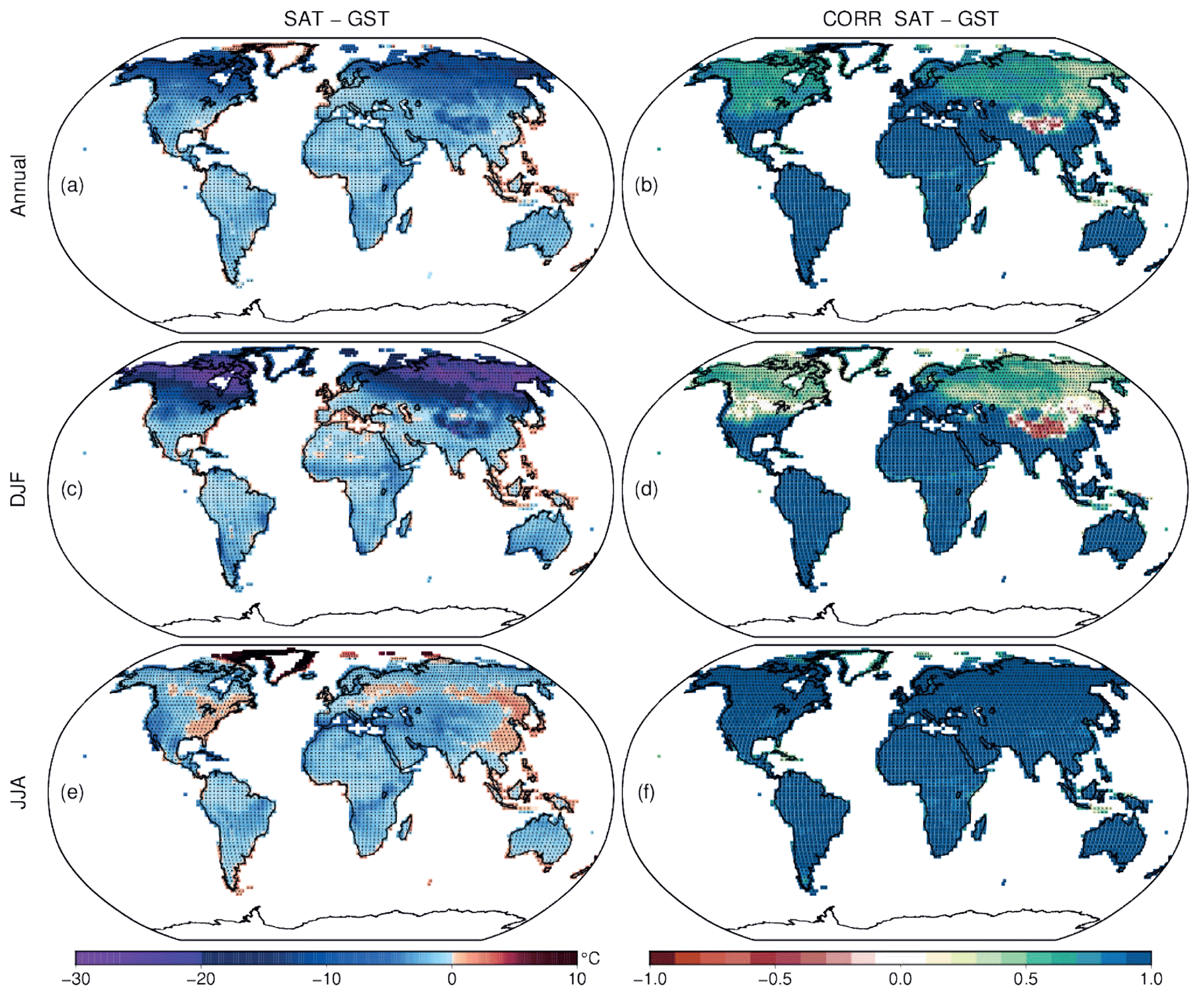
Figure 2(a) Annual, (c) DJF and (e) JJA spatial distribution of SAT minus GST differences during the 850–2005 CE period. (b) Annual, (d) DJF and (f) JJA spatial distributions of the correlation coefficients between SAT and GST for the same period. Black dots indicate that 80 % of the members within the ALL-F ensemble deliver statistical significance (p<0.05).
The spatial variability of the relationship between SAT and GST gives further insights into the role of different processes on the SAT–GST coupling. Figure 2 shows the spatial distribution of the differences between mean LM SAT and GST as well as the correlation coefficients for the annual, DJF and JJA averages in the ALL-F ensemble. In the case of the annual temperatures (Fig. 2a), GST is generally warmer than SAT with the differences being low over most of the globe (less than 2 ∘C) except in the NH mid- and high-latitude areas where the differences are higher (up to 15 ∘C). The correlation maps (Fig. 2b) provide a similar pattern with high and significant values over most of the globe (>0.8 in regions located between 45∘ N and 90∘ S) and lower correlations over NH mid- and high-latitudes, especially over eastern Siberia. Similar behavior is seen in the DJF season although it is more pronounced. During these months, GST is much warmer than SAT, reaching differences up to 30 ∘C in the northernmost parts of North America and Eurasia (Fig. 2c). Differences are smaller at mid- and low-latitudes. The influence of the ocean over coastal areas providing larger SAT relative to GST is noticeable. Similarly, the correlation is lower over the northern snow covered areas (Fig. 2d), while over the rest of the globe it remains high. In contrast, Fig. 2e, f show that during JJA, when the snow cover is scarce, the SAT–GST coupling is strong globally with temperature differences lower than 2 ∘C and high correlation coefficients (>0.9). Consequently, the role of snow cover in decoupling SAT and GST is highlighted. Positive correlation values are low over borderline areas where snow cover is more variable, which produces variability in the SAT–GST offset and thereby alters the covariance structure. Close to these areas in central Asia the high negative correlation within the Tibetan Plateau is noteworthy (see discussion below).
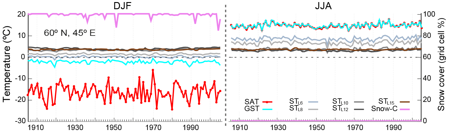
Figure 3Evolution of DJF and JJA SAT, GST, STL6, STL8, STL10, STL12 and STL15 and the percentage of snow cover during the 1900–2005 CE period for a grid point from the ALL-F2 simulation (northeast of Russia; 60∘ N, 45∘ E) where snow cover is characteristic during the cold season. Dashed lines indicate 0 ∘C.
Figure 3 illustrates the SAT–GST decoupling due to the snow cover at the local scale for a particular grid point as an example. The grid point is located over a region with considerable snow cover during the boreal cold season (northeastern Russia). The DJF and JJA evolutions of SAT, GST and ST at different depths and the snow cover for the last 105 years from the ALL-F2 simulation are shown. Note that in DJF snow covers 100 % of the grid cell during almost the whole period. Thus, the soil is insulated and the difference between SAT and GST is ∘C on average. The temperature of the deeper layers is presented in order to illustrate the amplitude attenuation and phase shift with the depth of the temperature signal. Note that during DJF, GST is only slightly below 0 ∘C, and the agreement of its variations with those of SAT is only noticeable in the largest changes of both, while STL6 and deeper STs are above 0 ∘C. In JJA, SAT and GST are very similar and their low frequency variability propagates to deeper levels, all above 0 ∘C.
Some aspects of the SAT–GST spatial distribution deserve further attention. One of the most noteworthy of these is the fact that over the Tibetan Plateau region temperature differences between SAT and GST are as large as in the mid- and high-NH latitudes for both annual and DJF periods (Fig. 2a, c). However, SAT and GST are negatively correlated for annual and DJF seasonal resolution data (Fig. 2b, d), with the Tibetan Plateau being the only region of the globe where this occurs. Nevertheless, the correlation for JJA is positive and high (Fig. 2e). The nature of this opposite phase arises from discontinuous snow cover over this region and the very low air temperatures during DJF. Usually, the snow cover insulates the soil from the colder air, avoiding the heat exchange with the atmosphere (as shown in Fig. 3). Nevertheless, discontinuous snow cover only partially insulates the soil, leading to this particular SAT–GST interaction. Figure 4 displays this behavior for a grid point located over the Tibetan Plateau. SAT, GST, ST at different depths, snow cover and surface sensible heat flux (SHFLX) are shown. In DJF during periods of low snow cover the fraction of surface exposed to the atmosphere allows for energy exchange from the warmer soil to the colder air. Conversely, when snow cover is high, the large fraction of insulated soil reduces almost completely the heat transfer from the soil to the atmosphere. Therefore, with lower (higher) fractions of snow cover, higher (lower) heat transfer takes place with GST decreasing (increasing) and SAT increasing (decreasing). Indeed, there is a high negative correlation (−0.84; p<0.05) between the snow cover fraction and SHFLX which is the main way that energy dissipates within this region since latent heat fluxes (LHFLX) are negligible. Higher/lower albedo due to variations in snow cover fraction also contribute to the negative SAT–GST correlation over this region (not shown). Horizontal model resolution does not seem to be an issue since a higher resolution version of the model (Landrum et al., 2012) produces a similar behavior which other models of similar resolution do not show (García-García et al., 2016). During JJA in comparison, snow cover is negligible and SAT–GST coupling is consequently strong. Note that GST and all ST are above zero and GST is higher than SAT as it is warmed by radiative gain and the transfer of heat to the atmosphere, hence the positive correlation (0.5; p<0.05) between SAT–GST and SHFLX.
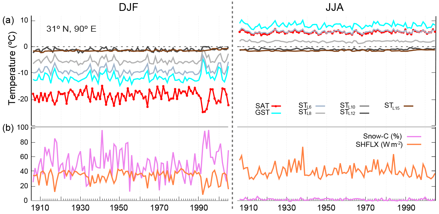
Figure 4(a) DJF and JJA evolution of SAT, GST, STL6, STL8, STL10, STL12 and STL15 for a grid point from the ALL-F2 simulation (Tibetan Plateau region; 31∘ N, 90∘ E) during the 1900–2005 CE period. Dashed lines indicate 0 ∘C. (b) Percentage of snow cover and surface sensible heat flux (SHFLX).
The spatial SAT–GST differences during JJA (Fig. 2e) depict other relevant aspects that have an influence on the SAT–GST relationship at relatively short timescales. SAT is generally colder than GST globally. However, for JJA, there are large areas inland, mainly located in the southeastern US, some parts of central and eastern Europe and eastern Asia, with warmer SAT relative to GST. Variations in LHFLX from DJF to JJA drive this effect. Figure 5 shows that the areas where LHFLX increases in JJA relative to DJF are related to the same areas where SAT is higher than GST in JJA (Fig. 2e). Therefore, there is a direct relation between the increase in evapotranspiration in JJA and the ground temperature response at these locations. The time series in Fig. 5 display this behavior for a grid point located over southeastern China. During JJA the surplus of energy due to higher solar radiation reaching the surface is mostly dissipated as latent heat leading to a net heat loss at the ground surface. Note the anticorrelation between the surface soil moisture and LHFLX (−0.46; p<0.05) during JJA as well as the large SHFLX values that occur when soil moisture is at its lowest and evapotranspiration is limited. Therefore, the high rate of LHFLX contributes to cool the surface and GST tends to be lower relative to SAT. Soil water content also exhibits large changes during JJA consistent with the large evapotranspiration (Fig. 5a) and provides a source of moisture that contributes to temperate SAT and cool GST. Large variations in evapotranspiration from DJF to JJA are also present at midlatitudes of the SH summer continents (America, Africa and Australia), although only a very limited impact on Fig. 2e is perceived, especially over the western coast. Over these regions, high incoming energy impinging the surface during SH summer (not shown) supports high rates of latent heat fluxes. However, as soil water becomes a limiting factor, more energy is dissipated as sensible heat and the ground surface is warmed. Therefore, GST experiences higher temperature than SAT on average. Figure 5 also shows high evapotranspiration over the tropical rainforest in America and Africa, both in DJF and JJA, which does not translate to positive SAT–GST differences. Over the rainforest, the energy fluxes at the surface do not vary significantly from DJF to JJA since incoming radiation is relatively constant throughout the year, and is transferred to evaporation and evapotranspiration within the canopy, while soils are well watered by precipitation to support the large amounts of evapotranspiration. This situation leads to a small range of variation in both SAT and GST with very small differences between them and higher GST relative to SAT.
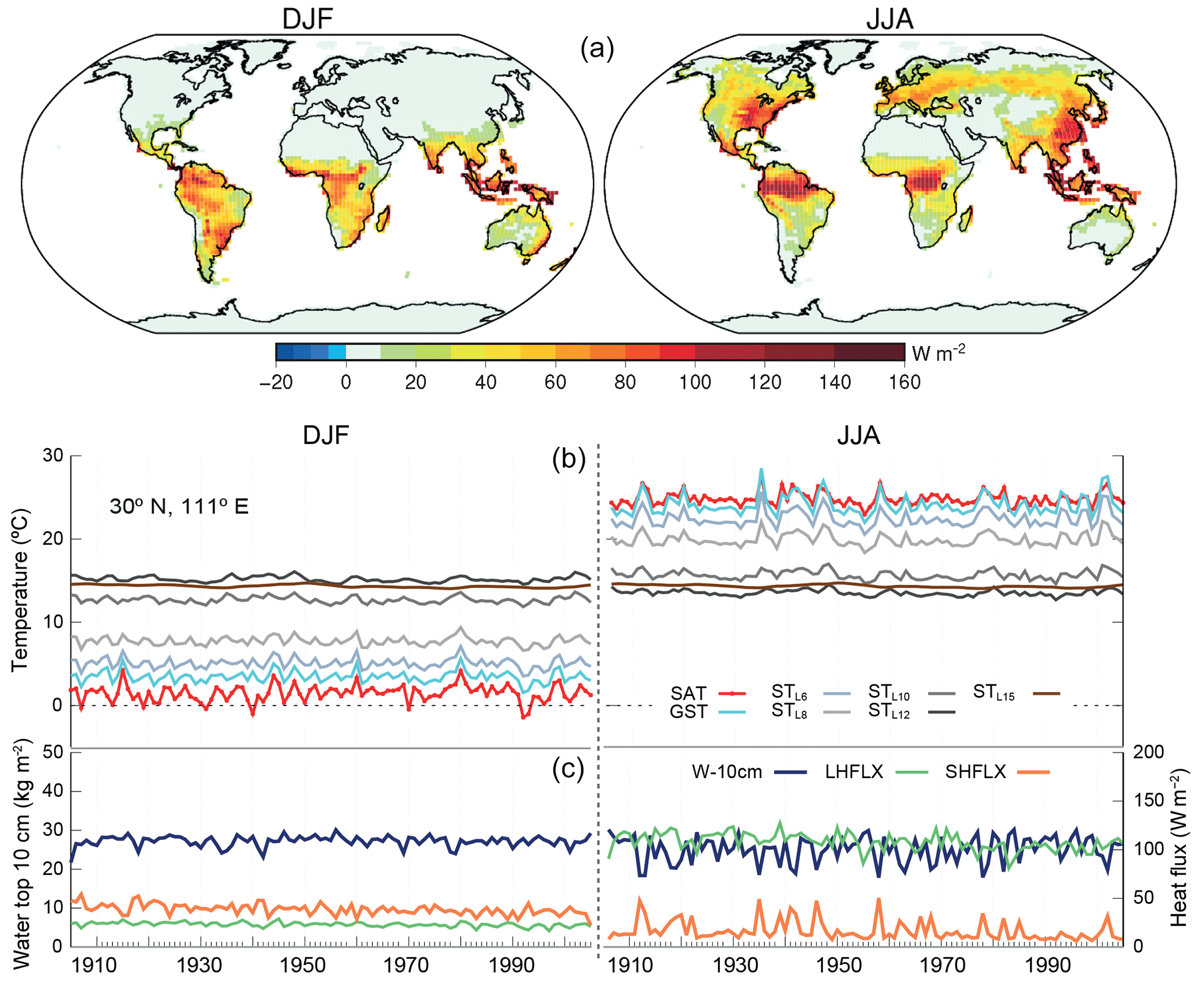
Figure 5(a) DJF and JJA average surface latent heat fluxes (LHFLX) over the 850–2005 CE period. (b) DJF and JJA time evolution of SAT, GST, STL6, STL8, STL10, STL12 and STL15 during the 1900–2005 CE period for a grid point from the ALL-F2 simulation (southeastern China, 31∘ N, 111∘ E). (c) Same for SHFLX, LHFLX and water content in the top 10 cm of soil (W−10 cm).
Figure 2a, c, e show similar higher SAT values relative to GST at some coastal areas in both JJA and DJF. During DJF the effect is mainly present in the NH midlatitudes, such as in most European coastal areas, both the east and the west coasts of North America, and in Japan and the east coast of China. During JJA, in comparison, this behavior is mostly seen in the SH midlatitudes, such as southern South America, South Africa and southern Australia. Interestingly, higher SAT relative to GST is also evident in some coastal areas over tropical regions; this applies for both JJA and in DJF, and is mainly observed over southeastern Asia, the southern areas of the Indian subcontinent, the Gulf of Guinea and some areas of South and Central America. In the CESM-LME the atmospheric grid box of the coastal areas is partitioned into land and ocean fractions. For the areas with sea ice formation, an additional sea ice fraction is considered (Neale et al., 2012). This configuration of the coastal grid points leads to a partition of the energy fluxes at the surface into those of the land fraction and those of the ocean fraction. During the cold season, partitioning such as this determines the higher SAT warming relative to GST, as the relatively low net radiation that impinges the surface at mid- and high-latitudes limits the ground surface heating as well as the energy fluxes out of the land surface fraction. In contrast, the energy fluxes from the ocean surface to the air above are large, primarily as a result of the temperature difference between the water and the comparatively colder air above. The dissipation of energy from the ocean fraction to the atmosphere warms the air, so the net effect is higher SAT relative to GST in the winter season. Over the tropical coasts that exhibit the same behavior, the energy fluxes out of the ocean fraction of each grid point also contribute to the higher warming of the air relative to the ground surface. Nevertheless, at these locations high rates of evapotranspiration all year long also play an important role as they generate evaporative cooling of the ground surface, as seen in the example described in Fig. 5.

Figure 6(a) Annual, (c) DJF and (e) JJA spatial distribution of GST minus STL8 differences during the 850-2005 CE period. (b) Annual, (d) DJF and (f) JJA spatial distribution of the correlation coefficients between GST and STL8 for the same period. Black dots indicate that 80 % of the members within the ALL-F ensemble deliver statistical significance (p<0.05).
The different examples used to illustrate the most important processes that may influence the air and soil temperature relationship at short timescales also depict relevant information about the propagation with depth of the annual cycle. For instance, at the grid point located over southeast China in Fig. 5, both in DJF and JJA, the temperature offset between contiguous levels is noticeable with a gradient of about 5 ∘C in the first meter of the ground and of about 10 ∘C down to the lowest level. Comparable pictures with some differences in the magnitude of gradients can be seen in the previous figures.
Therefore, it is interesting to also understand the propagation of temperature below the surface. GCMs simulate purely conductive regimes, and the temperature variations that propagate to deeper soil layers are established at or near the ground surface (Smerdon et al., 2003). Thus it is important to asses the propagation of the temperature signal within the shallow subsurface. This issue is addressed by analyzing the relationship between GST and STL8.
Figure 6a provides a spatial view of the temperature differences between GST and STL8 for annual, DJF and JJA periods. The correlation is also shown in the right panels. SAT–GST differences, for DJF and JJA show the yearly cycle of temperature with negative (positive) SAT–GST for the NH (SH) in DJF and vice-versa for JJA, illustrating the conductive regime within the shallow subsurface. The annual temperature differences are low and the correlation is high almost globally as it is the balance between the respective patterns in JJA and DJF. However, the northernmost part of the globe exhibits larger temperature differences (between 4 and 5 ∘C) and lower correlation coefficients. The DJF and JJA patterns show that the annual offset and correlations for this part of the globe are mostly the result of the larger weight of those in JJA given that, during these months, the temperature differences for a latitudinal band at ca. 60–70∘ N are as large as 15 ∘C and the correlation coefficients are close to zero. García-García et al. (2016) describe a similar behavior in some of the GCMs used in their analysis, detected over areas where frozen ground persists during JJA. Indeed, the nature of the large departure in the temperature response at the shallow subsurface at these locations arises from non-conductive processes related to latent heat release/uptake of freezing and thawing of the water content above a depth of 1 m that may account for the subsurface heat transfer (Kane et al., 2001).
To illustrate this mechanism, Fig. 7 shows the temperature evolution of SAT, GST and ST at different depths as well as the soil ice content (SIC) in the upper soil layers for a grid point located in the north of Canada. Over these areas the SIC in the upper 1 m of soil increases (decreases) during the cold (warm) season. During JJA, SAT and GST increase/decrease at the same rate since no ice is present at the ground surface so it is warmed by radiative gain and heat is transferred to the atmosphere. However, for deeper soil layers, the energy available is employed to melt the SIC (note the lower SIC in L6 during JJA relative to DJF), and latent heat is required so that these layers do not experience a temperature increase like the shallowest layers. Therefore the temperature at L8 (∼1 m depth) is kept below/near 0 ∘C during the warm season due to the zero-curtain effect (Outcalt et al., 1990), while GST is centered around 12 ∘C, leading to differences of ca. 15 ∘C between GST and STL8 and a low correlation coefficient (0.28 for this grid point) during JJA. In turn, during DJF, SAT sits around −35 ∘C and the frozen ground experiences skin temperatures of about −8 ∘C and of about −4 ∘C at a depth of 1 m. Consequently, the temperature offset between GST and STL8 is largest in JJA. As a result, there are some non-conductive processes associated with permanent frozen soils in the shallow subsurface that are included in the CLM4 parameterization (Lawrence et al., 2011) and that play an important role in heat transport. The higher SIC in L8 during JJA relative to DJF (Fig. 7) arises from the fact that freezing of the active layer begins in late autumn and, due to the release of the latent heat of fusion, the freezing front is inhibited (Hinkel et al., 2001) and only reaches L8 in spring when SIC at this layer peaks. Then, as the thawing front penetrates downward in JJA, ice in the shallowest soil is melted, but it does not reach L8 until autumn when SIC at this layer is lowest. Therefore, due to the thawing–freezing processes, seasonal changes at the upper and deeper subsurface levels are phase-shifted.
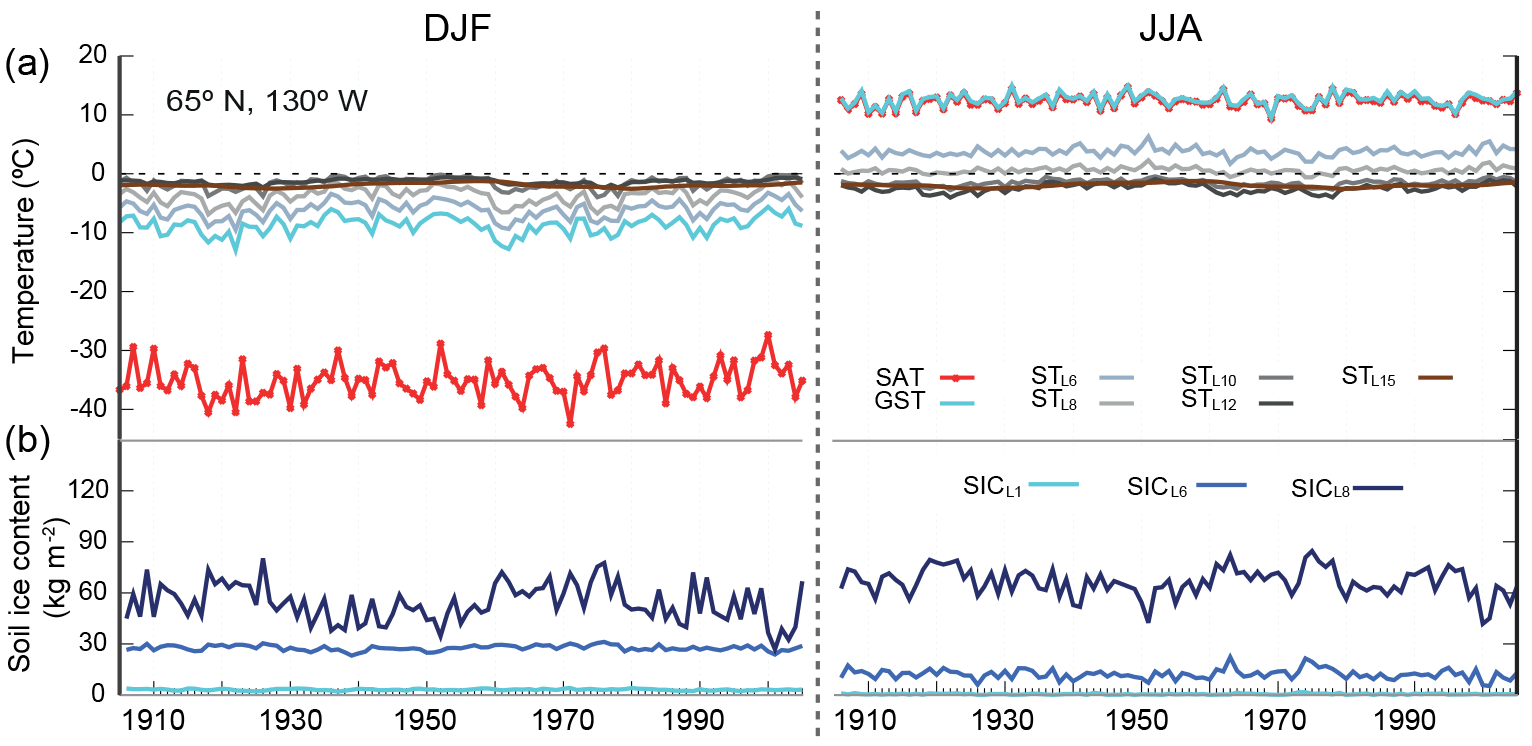
Figure 7(a) DJF and JJA evolution of SAT, GST, STL6, STL8, STL10, STL12 and STL15 during the 1900–2005 CE period for a grid point from the ALL-F2 simulation located in the north of Canada (65∘ N,1 30∘ W), an area with permanent frozen soils. Dashed lines indicate 0 ∘C. (b) Soil ice mass content (SIC) in the L1, L6 and L8 soil layers.
4.1 SAT–GST long-term changes
The mechanisms that have been described have an impact on the coupling between SAT and GST at short timescales but they do not affect the long-term SAT–GST association if they are stationary as its influence would be constant at long timescales. However, if such mechanisms experience variations with time, the SAT–GST relationship would also change over time. Thus, the thermal signature imprinted in the subsurface would not be representative of the long-term SAT variations (Bartlett et al., 2005). Figure 1b illustrates the existence of a constant offset between SAT and GST within the preindustrial period that changes during the industrial period indicating variation in the long-term SAT–GST relationship. This may be relevant in the interpretation of borehole climate reconstructions because it may induce a long-term decoupling between SAT and GST in the CESM-LME. At a global scale, the changes in the long-term SAT–GST offset have an impact of about 0.05 ∘C (Fig. 1a, b); thus, they do not seem to be very relevant at these scales. However, the impact could be larger for other GCMs with higher climate sensitivity or a different representation of surface processes that may contribute to decouple GST from SAT (e.g., snow cover). Similarly, within the CESM-LME simulations, impacts on decoupling may be important at regional or local scales.
To examine the spatial distribution of the long-term SAT and GST evolution during industrial times, we evaluate the linear trends of both temperatures independently during this period at every land model grid point. Besides the ALL-F ensemble, we also considered the anthropogenic single-forcing ensembles (Fig. 8), bearing in mind their potential influence on the processes that modulate the relationship between SAT and GST, such as variations in snow cover, soil moisture and albedo, among others. The results in this section are shown considering information from all members of the ensembles (see details in Table 3). For specific examples, one of the members will be used as indicated accordingly in figure captions.
Figure 8a, b describe a predominant warming for both SAT and GST in the ALL-F ensemble with the largest values distributed over northwest North America, north and central Eurasia, northeast Africa and southern South America. Interestingly, there are also regions showing negative trends like southeastern China, the north of the Black and Caspian sea regions, Pakistan, some relatively small central and southern areas of Africa and Brazil. The warming trend pattern can be explained to a large extent if the 1850–2005 trends are calculated on the basis of the GHG-only ensemble (Fig. 8c, d) which is consistent with the global warming pattern due to the influence of GHGs (Hartmann et al., 2013). Indeed, if only the contribution of GHGs is considered, the warming would be higher and globally distributed. Figure 8 also indicates that the cooling in the ALL-F ensemble is mainly driven by the contribution of the LULC and OZ/AER external forcings. For instance, the cooling trends over the Baltic Sea and the north of the Black and Caspian seas that dominate the SAT and GST cooling trends during the industrial period in the ALL-F ensemble are the result of the influence of LULC changes (Fig. 8e, f) with additional contributions of OZ/AER (Fig. 8g, h). In addition, the negative trends of both SAT and GST over some areas of Africa, as well as over the northeast of Brazil, are also detectable in the LULC-only ensemble (Fig. 8e, f). Similarly, the OZ/AER-only ensemble also contributes to the cooling over Brazil, and the strong negative trends observed in southeast China in the ALL-F ensemble are clearly identifiable in this ensemble (Fig. 8g, h).
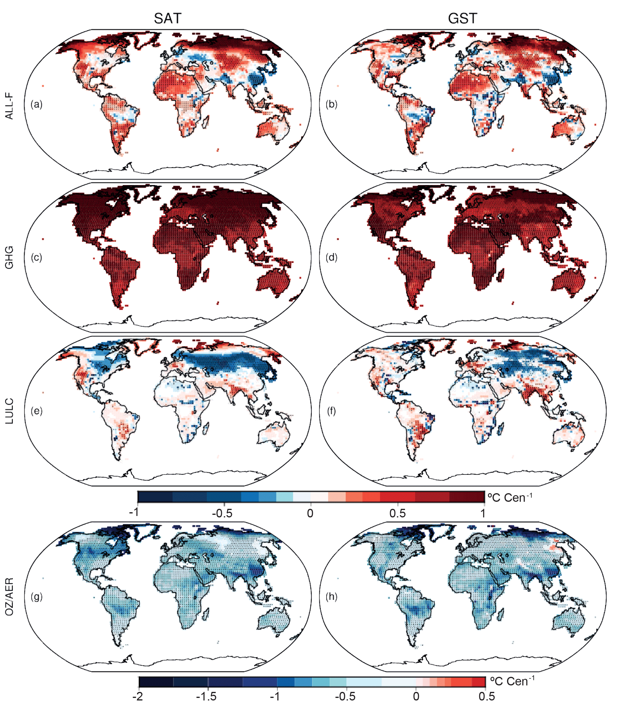
Figure 8Spatial distribution of the linear trends in the industrial period for the ALL-F (a, b), GHG-only (c, d), LULC-only (e, f) and OZ/AER-only (g, h) ensembles for SAT (a, c, e, g) and GST (b, d, f, h). Trends are indicated in Celsius century−1. Dots indicate that 80 % of the ensemble members agree in delivering significant trends at a grid point in the case of the ALL-F ensemble. For the GHG-only and LULC-only ensembles, dots indicate that at least two of the three ensemble members agree in delivering significant trends for a grid point, whereas for the OZ/AER-only dots indicate that both of the ensemble members deliver significant trends. Note the different scale for OZ/AER-only.
Although the general pattern of cooling/warming during industrial times is broadly similar for SAT and GST, with a spatial pattern correlation of 0.60, 0.64, 0.38 and 0.53 in the ALL-F, GHG-only, LULC-only and OZ/AER-only ensembles, respectively, it differs substantially in some regions. Note that there are considerable differences in the amplitude of warming trends in SAT and GST over Fennoscandia as well as at the northernmost part of North America in the ALL-F ensemble (Fig. 8a, b). Similarly, over some areas of central and eastern Europe, SAT and GST industrial trends have different sign. There are also considerable differences in the amplitude of the cooling in SAT and GST over northeastern Brazil. Such dissimilar behaviors of SAT and GST during the industrial period are connected to variations in the energy fluxes at the surface in response to changes in the land surface characteristics due to the influence of the external forcings during this period.
For a more detailed analysis of the SAT and GST long-term relationship, a two-phase regression model (Sect. 3) was applied at every land model grid point to the SAT–GST differences in the ALL-F, GHG-only and LULC-only ensembles (Fig. 9). This allows for the analysis of long-term changes in the coupling without assuming any a priori condition on their time of occurrence and also to separately analyze the contribution of the different forcing factors and the temporal consistency among them. In the case of the OZ/AER-only ensemble, since this set of simulations spans from 1850 to 2005 CE, linear trends are only shown for the industrial period (Fig. 10). Figure 9a shows the year of change for the three ensembles; changes significant for 80 % of the ensemble members are shown exclusively in Fig. 9b. The three ensembles show dates of change that span the whole millennium. However, significant changes only occur during the last centuries. Two-phase regression allows for identification of the fact that times of change in most regions take place prior to 1850, during the 18th and even the 17th century (e.g., India) in the ALL-F. Trends before the change are not significant in any of the ensembles (not shown). Trends after the change are shown in Fig. 9c; significant areas in at least 80 % of the ensemble members are exclusively shown in Fig. 9d. Note that large positive and negative trends in Fig. 9c coincide with the significant dates of change occurring during the last centuries of the LM.
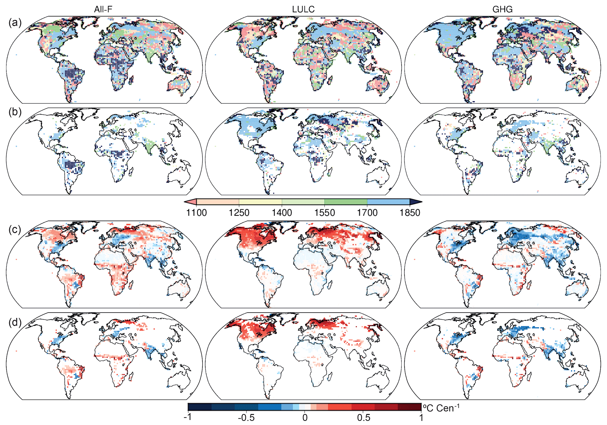
Figure 9Spatial distribution of the two-phase regression results for SAT minus GST in the ALL-F2, LULC1 and GHG1 ensembles as examples: (a) dates (years) of change; and (c) trends after the year of change. (b) and (d) are the same as (a) and (c) but only for areas where at least 80 % of the ensemble members show significant changes. Trends before the year of change (not shown) are not significant in any of the ensembles. Significance (p<0.05) is obtained based on an F test (t test) for year of change (trends) following Solow (1987). Significance also accounts for autocorrelation (Trenberth, 1984). Note that the spatial window has been modified to enhance visualization of land areas.
In general, annual SAT minus GST yields negative values (as shown in Fig. 2a) with the exception of the coastal areas as explained in Sect. 4. Thus, for continental areas (SAT–GST < 0), positive (negative) trends indicate that differences tend to get smaller (larger) in absolute values, whilst the opposite is true for the limited coastal areas where SAT–GST differences are positive. Figure 1b allows for visualization of this behavior. Note the positive trend after the change when the difference between SAT and GST anomalies becomes smaller with time. Regionally, several circumstances account for impacting SAT–GST long-term coupling. On the one hand, decreasing SAT–GST differences over land may emerge from two conditions. Firstly, when there is a higher warming rate of SAT relative to GST as depicted in Fig. 8a, b over the northernmost part of North America, Fennoscandia, northeast Russia and some areas of central Eurasia. Secondly, when there is a cooling of both SAT and GST but the latter decreases at a higher pace as described in Fig. 8a, b for the northeastern Brazilian region and some areas of Africa. These two scenarios are represented in Fig. 9c for the ALL-F, with positive trends over these regions after the change. On the other hand, the increase in the SAT–GST difference either arises from the effect of rising GST in the presence of stable/decreasing SAT or due to the higher warming rate of GST relative to SAT. The former case is displayed in Fig. 8a, b for central and eastern European areas as well as the eastern US, whereas the latter is found over the Indian subcontinent and southeastern Asia. Note that both cases are represented in Fig. 9c (ALL-F) with negative trends.
Trends from the GHG-only and the LULC-only ensembles help with understanding the relative contributions to the long-term variations seen in the ALL-F simulations. For instance, the GHG-only ensemble shows similar positive trends to the ALL-F (Fig. 9c) over northern North America, Fennoscandia, northeast Russia and central Eurasia, although with a much larger magnitude and geographical extension. Correspondingly, negative trends after the change in the LULC-only ensemble are comparable to those in the ALL-F for central and eastern Europe, the eastern US, the Indian subcontinent and southeastern Asia. Additionally, the positive values over Brazil, as well as over central and southern Africa in the ALL-F, are also depicted in the LULC-only ensemble. Most of these changes are robust in 80 % of the ensemble members (Fig. 9d).
Interestingly, the two-phase regression analysis does not expose any variation in the SAT–GST long-term relationship over southeastern China, where the linear trends during the industrial period show a relatively strong decrease in both SAT and GST in the ALL-F and the OZ/AER-only ensembles (Fig. 8a, b, g, h). Furthermore, the linear trend of SAT–GST differences during industrial times for the OZ/AER-only simulations (Fig. 10) does not exhibit any SAT–GST decoupling over this region either. This suggests that the dominant effect of OZ/AER forcing on the SAT and GST responses over this region is not affecting their long-term coupling. Nonetheless, Fig. 10 illustrates some interesting aspects of the SAT–GST relationship in the OZ/AER-only ensemble, such as the negative contribution to the SAT–GST trends over North America, northern Europe, the Tibetan Plateau and central Asia. Additionally, the positive trends over northern Siberia are also notable, as well as the positive values over some relatively small areas of central and eastern Africa, the coast of Angola and eastern Brazil. Although the bulk of these SAT–GST responses depicted in Fig. 10 do not translate to SAT–GST long-term decoupling in the ALL-F ensemble, they play an important role in either counteracting the influence of other external forcings or contributing to decoupling-related processes over some regions.
The following paragraphs aim at providing an insight into the relative contribution of the individual forcings and the associated physical mechanisms to the variations of the long-term SAT–GST association detected in Figs. 9 and 10.
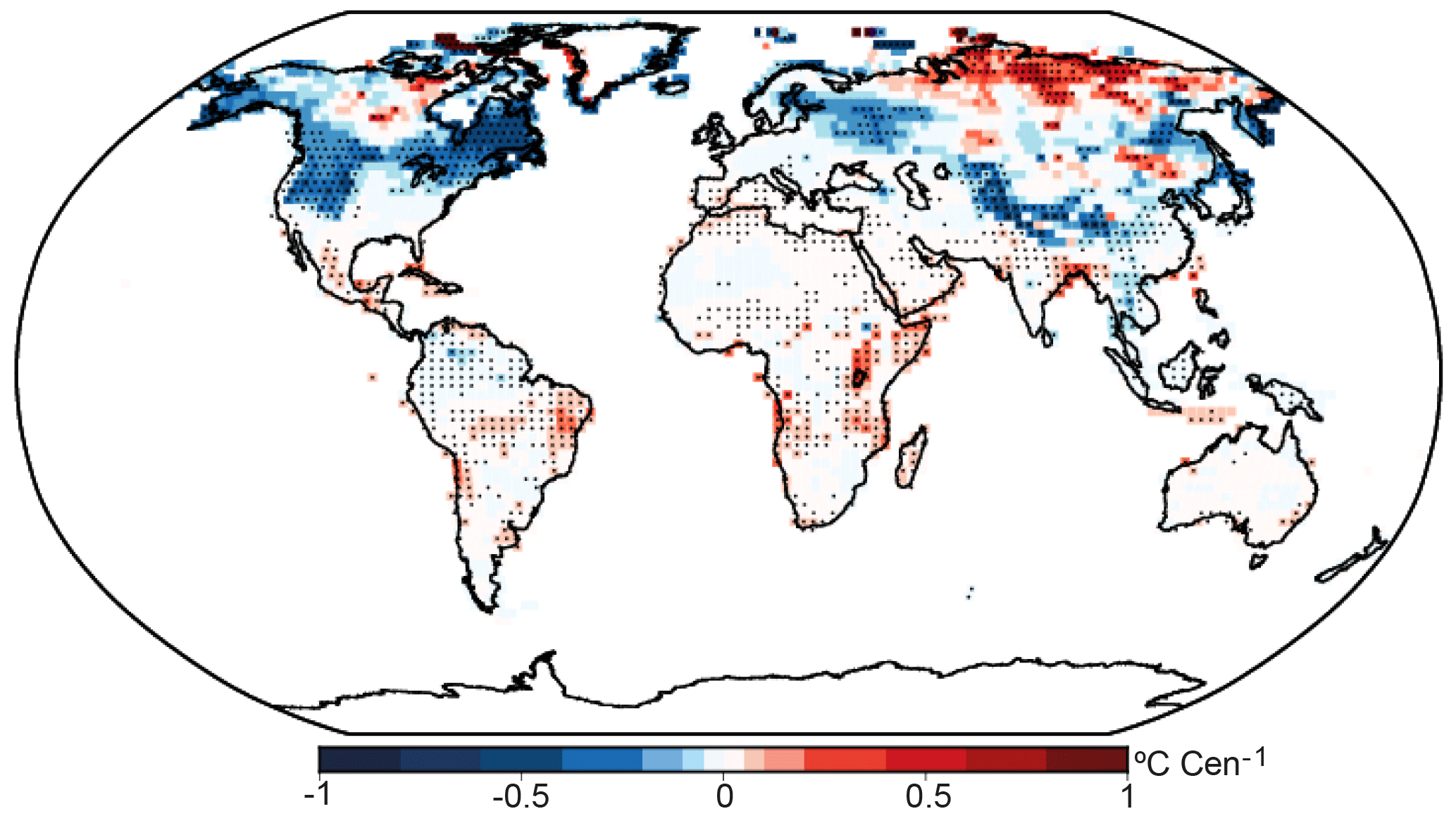
Figure 10Spatial distribution of the linear trends for SAT minus GST in the OZ/AER-only ensemble. Trends are indicated in Celsius century−1. Dots indicate agreement in both of the ensemble members.
In the cases of the long-term variations due to the LULC influence, changes in vegetation cover alter the radiative fluxes and water cycling at the surface due to the modification of the physical properties such as albedo, roughness and evapotranspiration (Pongratz et al., 2010). Figure 11 gives an example of how long-term changes in the energy fluxes at the surface due to LULC changes do impact the SAT–GST coupling at long timescales. It shows the 31-year low-pass filter outputs of SAT, GST, reflected shortwave radiation (RSW) and SHFLX evolution for a characteristic grid point over the Great Lakes region (US) where a warming of GST relative to SAT is simulated in CESM-LME during the industrial period. Results are shown for one of the members of the ALL-F, LULC-only, GHG-only and OZ/AER-only ensembles. Around 1800 CE SAT tends to decrease whereas GST tends to increase in both the ALL-F and LULC-only simulations, while GHG-only and OZ/AER-only simulations do not display the same behavior that produces larger differences between SAT and GST represented by negative trends in Fig. 9c. At the same time, RSW and SHFLX exhibit large long-term variations in the ALL-F and LULC-only simulations. Therefore, this modification of the long-term SAT–GST relationship is clearly a response to LULC changes. Such variations in the surface energy fluxes over this region are likely a response of vegetation replacement from forested areas to grassland or croplands. Forested landscapes dissipate SHFLX more efficiently to the atmosphere due to a higher surface roughness than open fields (Jackson et al., 2008). In addition, lower vegetation types have higher reflectivity than forests. All of the previously listed factors contribute to SAT decreases over these regions, especially in DJF. Furthermore, deforestation at mid- and high-latitudes tends to positively feedback with increases in snow cover (Anderson et al., 2011). These types of changes in LULC contribute to increase albedo, which is reinforced by changes in snow cover at these latitudes. Additionally, higher DJF snow cover tends to increase the insulation of the soil from the cold overlying air. The combination of these mechanisms lead to the observed temperature response of SAT and GST. This particular LULC process is important for corrupting the SAT–GST coupling at timescales relevant for the borehole theory (centennial) since the thermal signature recorded in GST during the industrial period would not be representative of the past long-term SAT variations in regions where this effect is dominant.
For the areas of central and eastern Europe, where a GST warming relative to SAT is also observed in Fig. 9c, the mechanisms are similar to those described in Fig. 11, because these areas were also subject to an intense transformation from forested areas to cropland prior to the beginning of the industrial period according to the LULC forcings considered in the CESM-LME (Hurtt et al., 2009; Pongratz et al., 2008).
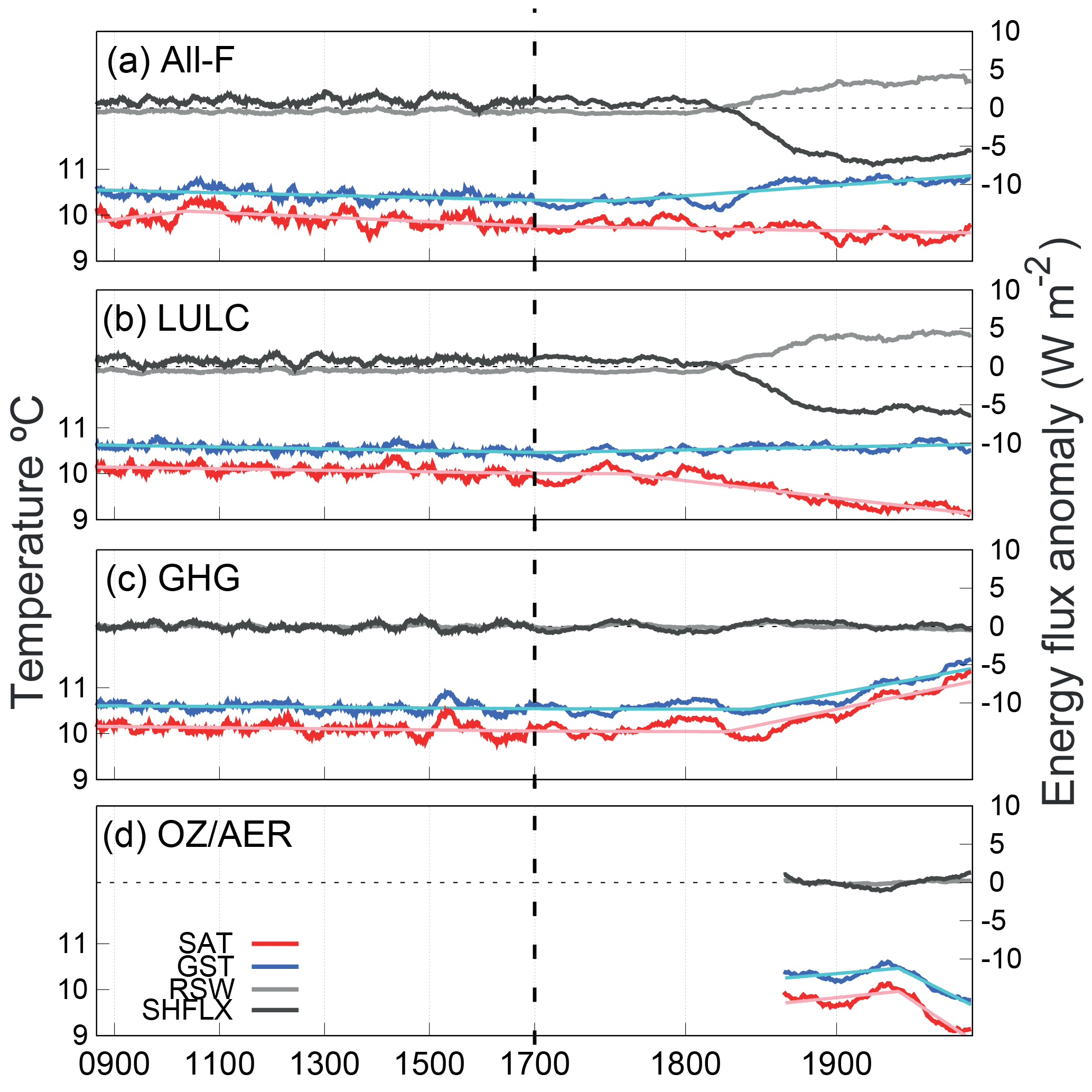
Figure 11LM evolution of SAT, GST, reflected shortwave radiation (RSW) and surface sensible heat flux (SHFLX) for a grid point located at 40∘ N, 82∘ W in the south of the Great Lakes, US, in the ALL-F2, LULC1, GHG1 and OZ/AER1 simulations. The left axes correspond to SAT and GST, while the right axes correspond to the energy fluxes at the surface. Note that for the energy fluxes the anomalies with respect to 850–2005 CE are shown, whereas for temperature absolute values are presented. All series are 31-year moving average filter outputs. For SAT and GST the result of the two-phase regression model is displayed with thin solid lines. Note the change in timing on the x axis after 1700 CE.
Changes in vegetation cover are also important for the long-term SAT and GST temperature differential response over tropical regions, although the driving mechanisms are different from those at mid- and high-latitudes (Lee et al., 2011) and they deserve to be considered. In the northeast of Brazil, both SAT and GST have negative trends in both the ALL-F and the LULC-only ensembles during the industrial period (Fig. 8a, b, e, f). However, the decrease of GST is much larger than that of SAT as represented in Fig. 9c with positive trends after the change in both ensembles.
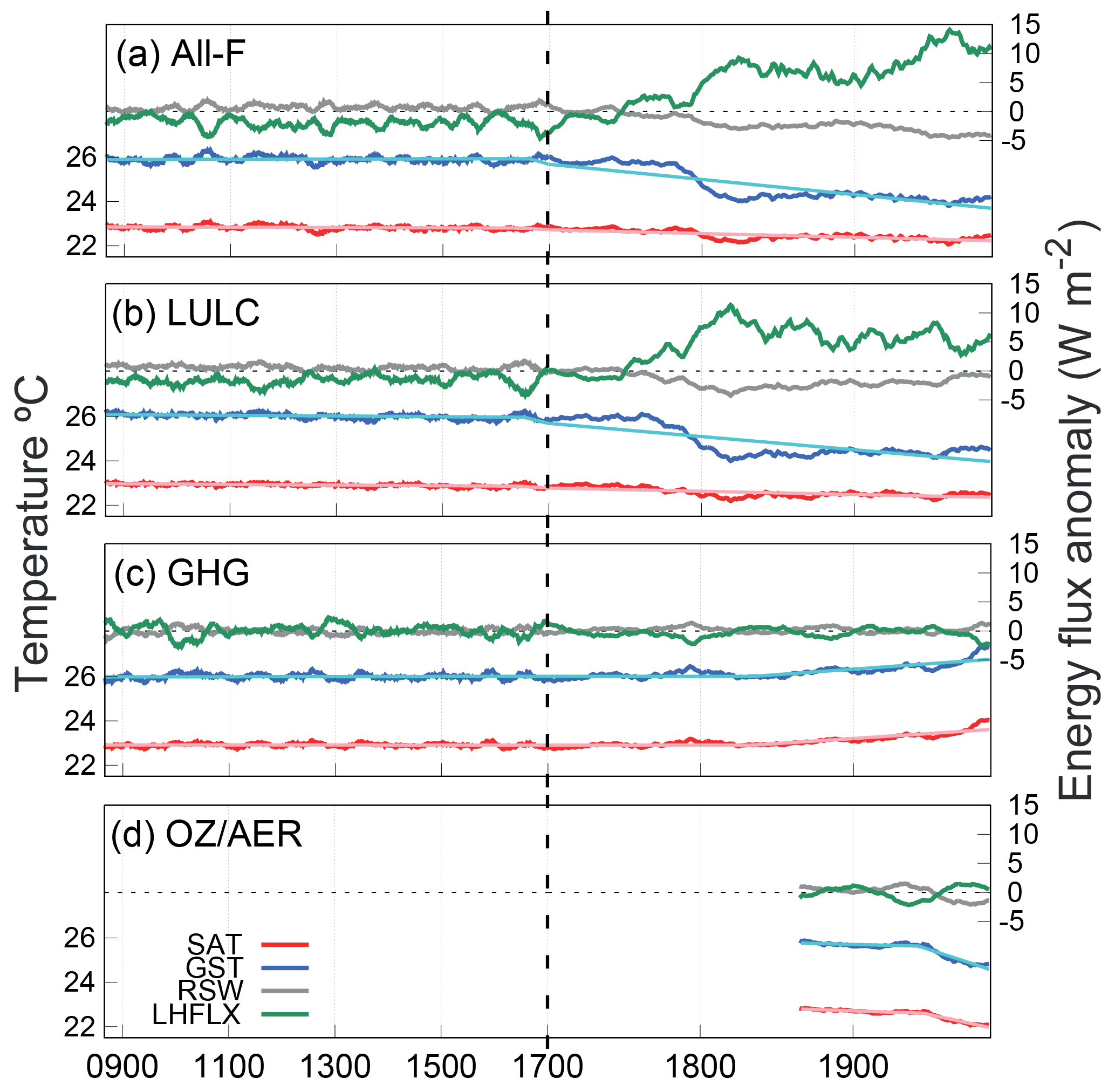
Figure 12The same as in Fig. 11 but for a grid point located at 12∘ S, 40∘ W in northeast Brazil. LHFLX is also represented instead of SHFLX.
Figure 12 shows the temporal evolution of SAT, GST, RSW and LHFLX for a grid point located in northeast Brazil. At the end of the 18th century, GST drops sharply whereas SAT slightly decreases. Similarly, RSW and LHFLX simultaneously experience significant changes as a result of the modification of the surface characteristics. Such changes are present solely in the All-F and LULC-only simulations, whereas the GHG-only and OZ/AER-only simulations show no differences in their evolution. The changes observed at this location in the energy fluxes likely correspond to transitions from open lands to a forested area (reforestation or afforestation) leading to lower albedo and higher evapotranspiration rates as is shown in Fig. 12. This situation leads to an apparent long-term cooling of GST relative to SAT at this location. The temperature response over this area is influenced by different mechanisms. First, the conversion from lower-type to higher-type vegetation reduces the solar radiation that impinges on the surface and GST decreases due to a radiative effect. Second, forested lands usually have lower albedo and thus absorb more shortwave radiation (Zhao and Jackson, 2014). This surplus of energy is balanced by the increase in transpiration; consequently, GST also decreases by a non-radiative process. The latter is especially important in humid climates (von Randow et al., 2004) such as the one in this example. According to these results, there is a net heat loss at the ground surface with a higher decrease in GST relative to the overlying air. The SAT–GST coupling becomes strong again after the new vegetation cover reaches a stable state by the mid 20th century. For the African areas, where there is also a cooling of GST relative to SAT (Fig. 9c in the ALL-F and LULC-only ensembles), the mechanisms are comparable to those described for Fig. 12.
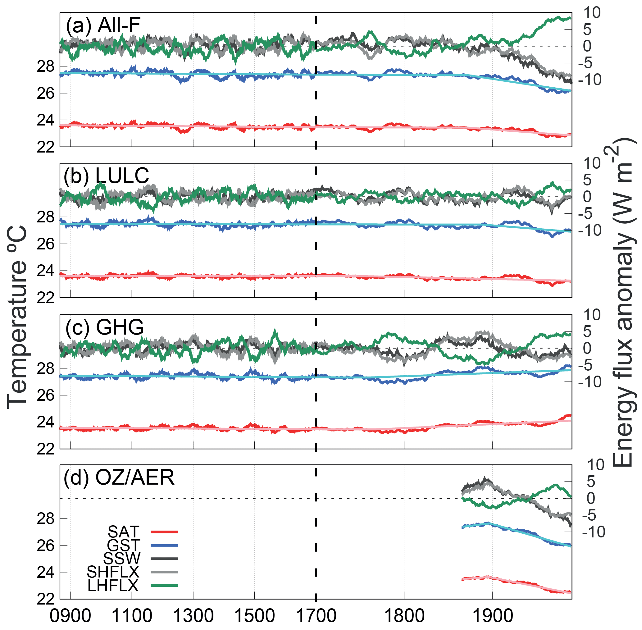
Figure 13The same as in Fig. 11 but for a grid point located at 2.5∘ N, 33∘ E over Uganda. Note that the incoming shortwave radiation at the surface (SSW) is represented instead of RSW and both LHFLX and SHFLX are shown.
Over some of these tropical regions, there is also a contribution from the OZ/AER forcing to the SAT–GST response. Note that Fig. 10 shows positive trends over Uganda, the coast of Angola and over eastern Brazil, which is also noticeable in Fig. 9c. In these regions, the incoming solar radiation is reduced due to the effect of aerosols, which are an important element for cloud formation and contribute to a higher reflectivity of solar radiation (Tao et al., 2012). The description of the specific processes related to aerosol–cloud interaction goes beyond the scope of this study. Therefore, only the influence on the energy balance at the surface is addressed. As lower shortwave radiation impinges the surface, the energy gain decreases and the ground surface heating is consequently lower. The reduction in the energy gain at the surface is compensated for by a lower dissipation via sensible heat, whereas the fluxes of latent heat remain relatively constant or even increases in some areas due to higher moisture as a result of increased precipitation. This mechanism is illustrated in Fig. 13 for a grid point located in the Uganda region. Note in the ALL-F simulation, the reduction in incoming shortwave radiation (SSW) after 1900 CE leads to a decrease in SHFLX. Interestingly, for this location LHFLX experiences an increase at the same time as a result of increased precipitation (not shown); thus, this provides a source of moisture for evapotranspiration. This situation leads to a higher decrease in GST relative to SAT due to a net loss of energy at the ground surface. Similar SAT and GST responses are observed in the OZ/AER-only and LULC-only simulations, whereas in the GHG-only SAT and GST increase.
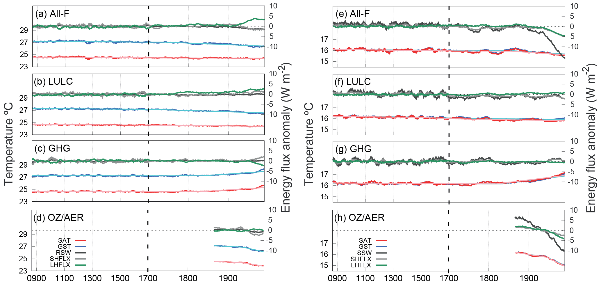
Figure 14The same as in Fig. 11 but for two different regions: northeast Brazil between 1–11∘ S and 47–35∘ W (a) and southeast China between 22–32∘ N and 103–122∘ E (b). For northeast Brazil RSW is represented whereas for southeast China SSW is shown instead. LHFLX and SHFLX are shown in both cases.
The SAT–GST decoupling processes described above for individual grid points are also important at larger spatial scales. Figure 14a shows an extension of the mechanism depicted in Fig. 12 including a larger area over the northeast of Brazil (between 1–11∘ S and 47–35∘ W). The negative trend since the 18th century is less accentuated for SAT than for GST (−0.14 and −0.53 ∘C century−1 respectively in the All-F simulation and −0.07 and −0.33 in the LULC-only ensemble) indicating a strong contribution of past LULC changes. The same air–subsurface temperature response occurs in other tropical and subtropical areas such as the east of Africa.
The regional analysis is extended to southeastern China in order to illustrate additional information about the influence of different external forcings on the SAT–GST relationship. As previously discussed, the negative trends for both SAT and GST over this region during the industrial period represented in the ALL-F and OZ/AER-only ensembles (Fig. 8a, b, g, h) do not entail a corruption of the SAT–GST long-term coupling. Figure 14b allows for insight into this particular effect and the role of the OZ/AER forcing on the air and soil temperature responses over this region during industrial times. The negative long-term trend within the industrial period is only seen in the ALL-F and the OZ/AER-only simulations. Similarly, in both of these simulations, there is a reduction in the RSW as well as in both the LHFLX and SHFLX. Conversely, the SAT and GST evolution during industrial times in the GHG-only and LULC-only simulations does not follow the same path depicted in the ALL-F, which highlights the dominant influence of OZ/AER forcing. In this case, the variations of the energy fluxes at the surface depend on the reduction of the incoming shortwave radiation as a response of the anthropogenic aerosol–cloud interaction rather than by modifications of the land surface properties. Therefore, the decrease in the energy that impinges the surface is balanced by a decrease in both the sensible and latent heat fluxes. Hence, the air–soil interactions are not significantly altered and the SAT–GST relationship remains stable.
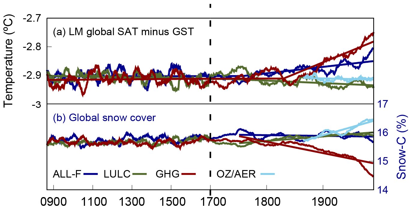
Figure 15(a) LM evolution of the global SAT–GST offset for the ALL-F2, LULC1, GHG1 and OZ/AER1 simulations. Straight lines indicate the long-term trend during the LM from a two-phase regression analysis except for the OZ/AER1 results that indicate a linear trend in the industrial period. The bottom panel illustrates the LM evolution of global snow cover percentage for the same ensemble members. Straight lines indicate the long-term trend within the 1750–2005 period except in the case of OZ/AER that only covers the 1850–2005 period. The period from 1750–2005 was selected in order to match the time span when the SAT–GST offset experiences the variation in the ALL-F2 simulation. All series are 31-year moving average filter outputs. Note the change in timing on the x axis after 1700 CE.
Although the majority of the important long-term variations in the SAT–GST relationship at regional and local scales observed in the ALL-F ensemble (Fig. 9c) are induced by LULC changes, there are some regions in which the GHG forcing is the main driver for long-term SAT–GST decoupling. For instance, the positive trends after the change over Fennoscandia, northeast Russia and the north of North America observed in the ALL-F ensemble can be explained to a large extent by the influence of GHG-only ensemble inasmuch as a broadly similar picture is portrayed over these regions in both ensembles (Fig. 9c). In the case of the GHG-only ensemble, the strong warming of SAT relative to GST over these regions is driven by the increasing air temperature during industrial times due to the positive radiative forcing of GHGs in the presence of a considerable long-term reduction in simulated snow cover. González-Rouco et al. (2009) showed that such a scenario would lead to a higher exposure of soil to cold winter air; therefore, the soil would partially record colder temperatures, which had previously been prevented by the snow cover insulating effect. In the ALL-F ensemble, this effect is damped as additional forcings that keep the snow cover relatively constant during industrial times are considered. For instance, the contribution of the OZ/AER forcing is particularly important for counteracting the effect of GHGs as it leads to colder climate conditions due to its negative radiative forcing. Note the strong negative trends in Fig. 10 over North America, northern Europe and the Tibetan Plateau that partially balance the effect of the GHGs over these regions. Nonetheless, in the ALL-F there is still an overall SAT warming relative to GST since the relatively stable snow cover is insulating the soil from a warmer SAT reducing the overall offset between them (Bartlett et al., 2005). Additionally, other processes can play some local roles in SAT–GST changes, such as CO2 fertilization generating increases in leaf area index (e.g., Amazon rainforest), which leads to higher evapotranspiration (Mankin et al., 2018) and GST cooling relative to SAT.
Figure 15 gives further insights into the interactions between anthropogenic forcings, their influence on global snow cover and consequently on the long-term SAT–GST relationship in the CESM-LME. The LM evolution of global SAT minus GST (top) and the annual global snow cover (bottom) for the ALL-F, LULC-only, GHG-only and OZ/AER-only simulations are shown for one member of each ensemble. Similar results are obtained if other members are selected. On the one hand, when the GHG-only ensemble is considered the global SAT–GST offset experiences a sharp long-term decrease in absolute value at the start of the industrial period as well as a strong long-term reduction in global snow cover. In fact, the correlation between changes in the SAT–GST offset and snow cover in the GHG-only ensemble member is high −0.93 (p<0.05). On the other hand, the overall effect of the LULC-only ensemble is a relatively small increase in the global snow cover mainly due to deforestation at mid and high latitudes as well as due to the negative radiative forcing of LULC as Earth's albedo increases (Myhre et al., 2013); this leads to a small increase in the global SAT–GST offset. In the same way, the OZ/AER-only ensemble shows an increase in global snow cover while the SAT–GST offset in industrial times exhibits a relatively slight increase. The interaction between different external forcings in the ALL-F ensemble leads to a relatively stable snow cover during the industrial period since the sharp decrease in snow, induced by the GHG forcing, is partially compensated for by the counteracting effect of the LULC and OZ/AER forcings. Additional forcings such as volcanic eruptions may also contribute to counteracting GHG effects at multi-decadal timescales (not shown). Consequently, in the presence of a warmer climate, there is a difference in the warming rate of SAT and GST in industrial times at a global scale in the ALL-F ensemble member (0.25 and 0.18 ∘C century−1, respectively). This scenario leads to the net effect of a long-term decrease in the SAT–GST differences starting around 1800 CE as discussed in Fig. 1 and as is also evident in Fig. 15.
This work evaluates the stationarity of the coupling between SAT and GST temperatures as simulated by the CESM in an ensemble of experiments spanning the LM. The initial motivation for this work is rooted on previous literature (García-García et al., 2016; González-Rouco et al., 2003, 2006, 2009) that addresses the realism of the borehole hypothesis for climate reconstruction, namely, that SAT and GST vary synchronously and that reconstructing past GST changes from borehole temperature profiles is a good proxy for past SAT variations. The use of the CESM-LME allows for the analysis of the influence of forcing changes on the SAT–GST covariability, both individually and as a group, by considering the different all-forcing and single-forcing ensembles. Additionally, having several experiment ensemble members for each given forcing type allows for the disentanglement of the effects of internal variability from those of the forcing response. Ultimately, the coupling between SAT and GST is assessed at a global and also at regional/local scales. This assessment requires the consideration of different mechanisms that contribute to SAT–GST variability within different climate types. In doing this, a variety of factors and conditions that contribute to the surface energy balance via different mechanisms are provided.
The CESM-LME shows that at global scale the SAT–GST coupling is strong above multi-decadal timescales since GST tracks SAT throughout the LM, as found in previous studies. However, in spite of the strong coupling, the CESM-LME also reflects that the SAT–GST relationship has not remained constant throughout the whole LM at these spatiotemporal scales. Hence, the nature of such variation is evaluated.
Globally, snow cover is the most important agent in modulating the connection between SAT and GST. Therefore the variation of the SAT–GST relationship described by the CESM-LME simulations should, in principle, be driven by variations in global snow cover. Nevertheless, the simulated snow cover remains relatively stable at the time when SAT–GST coupling varies; thus, this change cannot be solely explained by the influence of the snow cover. With this in mind, we explored, in some detail, different processes that may influence the SAT–GST relationship at different spatiotemporal scales. Firstly, we address processes acting at seasonal timescales that were identified from a spatial analysis of the SAT–GST differences and correlations. Secondly, the long-term evolution of the SAT–GST relationship is evaluated in the ALL-F, LULC-only, GHG-only and OZ/AER-only ensembles.
Several processes over different regions relevant during either DJF or JJA play an important role in impacting the SAT–GST coupling, such as snow cover over mid- and high-latitudes, discontinuous snow cover over the Tibetan Plateau region and seasonal variations in the energy fluxes at the surface. Although these processes are important for disrupting the SAT–GST relationship at seasonal scales, they have no implications on the long-term coupling if they are stationary. Nonetheless, if they experience variations with time the SAT–GST long-term relation may be impacted.
As discussed in Sect. 4.1 some of the anthropogenic external forcings have the potential to impose long-term variations on processes that regulate the relationship between SAT and GST. Among them, LULC changes are the most important of these forcings as they modify the energy fluxes at the ground–air interface, and consequently corrupt the SAT–GST coupling locally and regionally at various timescales. One example is the response to the deforestation processes triggered by the expansion of agriculture mainly during the industrial period at mid- and high-latitudes, where SAT and GST long-term coupling is impacted due to the variations in the albedo, surface roughness and hydrology. Similar decoupling processes related to LULC changes are found over different regions around the globe, such as those described in Sect. 4.1 over northeastern Brazil, and over some areas in Africa and the Indian subcontinent. All of these examples are driven by the long-term modifications of the energy fluxes at the surface, either from increased evapotranspiration, reduced energy dissipation via sensible heat or other factors. Besides these kinds of decoupling processes induced by individual forcings, the interactions of a variety of mechanisms and feedbacks from different external forcings can also exert an influence on the long-term SAT–GST relationship at different spatial scales. For instance, the effect of GHGs leads to a reduction of the snow cover during industrial times that is counterbalanced by the opposite effect of both LULC and OZ/AER forcings. As a consequence, the snow cover remains relatively stable over some regions during the industrial period in the presence of a warmer climate. This situation leads to a difference in the SAT–GST long-term evolution during the industrial period, since the snow cover insulates the soil from a warmer SAT. This effect is present over the NH high-latitudes of North America, Fennoscandia and northeastern Russia. Indeed, at a global scale, the combination of steady snow cover under warmer climate conditions is the dominant effect for explaining the variations in the long-term SAT–GST relationship.
Our findings indicate that the assumption of a strong relationship between SAT and GST may be impacted from local to regional scales by different mechanisms especially by the influence of LULC changes due to the modification of the energy balance at the surface. Therefore, the interpretation of temperature reconstructions from borehole measurements at these spatial scales must consider LULC changes as a source of possible bias. The effects of additional external forcings may also exert some influence on processes such as variations in the snow cover, hydrology and other land surface properties, which may in turn feedback on the SAT–GST long-term coupling. At a global scale, the influence of such local and regional decoupling processes is only ca. 0.05 ∘C; hence, the SAT–GST coupling at this spatial scale is supported by the CESM-LME.
The analysis using different GCMs may yield different levels of impacts. Overall, some consistency in the impacts among the available simulations of the LM with different GCMs can be expected. This is due to the fact that the external forcings considered in the PMIP3/CMIP5 LM simulations are similar (Schmidt et al., 2011) and should have a similar contribution to the extent that the impacts on the SAT–GST long-term relationship are mainly driven by the external forcings. Nevertheless, not all model simulations consider exactly the same set of forcings. Some consider land use land cover changes and aerosols, and other do not (Masson-Delmotte et al., 2013). In addition, different model climate sensitivities and differences in the representation of surface processes (e.g., snow cover or soil moisture) may also contribute to produce different responses. Even if the role of external forcings should be dominant in a long-term context, addressing this issues from a multi-model ensemble approach would help with understanding the uncertainties associated with all the factors of variation described above. The CMIP6/PMIP4 (Eyring et al., 2016; Jungclaus et al., 2017) offers an opportunity to explore better sensitivity to different models, as larger ensembles of the LM with a more systematic sampling of forcings and processes would be expected.
The results of this analysis are available from the authors upon request.
This study is part of CMA's PhD. The experimental design was set up by CMA and JFGR. CMA carried out the data processing, analyzed the results and wrote the paper. All of the other authors contributed to the analysis and discussion of the results and to writing the paper.
The authors declare that they have no conflict of interest.
This research was supported by an FPI grant (grant no. BES-2015-075019), from the
Spanish Ministry of Economy, Industry and Competitiveness. We gratefully
acknowledge the IlModels project, project no. CGL2014-59644-R. We also thank
Bette L. Otto-Bliesner for personal communications regarding several
aspects of the methodological design of the CESM-LME, as well as the
CESM1(CAM5) Last Millennium Ensemble Community Project and supercomputing
resources provided by NSF/CISL/Yellowstone.
Edited by: Jürg Luterbacher
Reviewed by: three anonymous
referees
Alexeev, V. A., Nicolsky, D. J., Romanovsky, V. E., and Lawrence, D. M.: An evaluation of deep soil configurations in the CLM3 for improved representation of permafrost, Geophys. Res. Lett., 34, L09502, https://doi.org/10.1029/2007GL029536, 2007. a
Ammann, C. M. and Wahl, E.: The importance of the geophysical context in statistical evaluations of climate reconstruction procedures, Climate Change, 85, 71–88, 2007. a
Anderson, R., Canadell, J., Randerson, J., Jackson, R., Hungate, B., Baldocchi, D., Ban-Weiss, G., Bonan, G., Caldeira, K., Cao, L., Diffenbaugh, N., Gurney, K., Kueppers, L., Law, B., Luyssaert, S., and O'Halloran, T.: Biophysical considerations in forestry for climate protection, Front. Ecol. Environ., 9, 174–182, https://doi.org/10.1890/090179, 2011. a, b, c
Bartlett, M. G., Chapman, D. S., and Harris, R. N.: Snow and the ground temperature record of climate change, J. Geophys. Res., 109, F04008, https://doi.org/10.1029/2004JF000224, 2004. a, b, c, d
Bartlett, M. G., Chapman, D. S., and Harris, R. N.: Snow effect on North American ground temperatures, 1950–2002, J. Geophys. Res., 110, F03008, https://doi.org/10.1029/2005JF000293, 2005. a, b, c
Beltrami, H. and Kellman, L.: An examination of short- and long-term air-ground temperature coupling, Glob. Planet. Change, 38, 291–303, https://doi.org/10.1016/S0921-8181(03)00112-7, 2003. a
Beltrami, H., González-Rouco, J. F., and Stevens, M. B.: Subsurface temperatures during the last millennium: Model and Observation, Geophys. Res. Lett., 33, L09705, https://doi.org/10.1029/2006GL026,050, 2006. a
Berger, A., Loutre, M.-F., and Tricot, C.: Insolation and Earth's orbital periods, J. Geophys. Res.-Atmos., 98, 10341–10362, https://doi.org/10.1029/93JD00222, a
Betts, R. A.: Biogeophysical impacts of land use on present-day climate: near-surface temperature change and radiative forcing, Atmos. Sci. Lett., 2, 39–51, https://doi.org/10.1006/asle.2001.0023, 2001. a
Betts, R. A., Falloon, P. D., Goldewijk, K. K., and Ramankutty, N.: Biogeophysical effects of land use on climate: Model simulations of radiative forcing and large-scale temperature change, Agr. Forest Meteorol., 142, 216–233, https://doi.org/10.1016/j.agrformet.2006.08.021, 2007. a
Bodri, L. and Cermak, V.: Borehole temperatures, climate change and the pre-observational surface air temperature mean: allowance for hydraulic conditions, Glob. Planet. Change, 45, 265– 276, https://doi.org/10.1016/j.gloplacha.2004.09.001, 2005. a
Brovkin, V., Claussen, M., Driesschaert, E., Fichefet, T., Kicklighter, D., Loutre, M. F., Matthews, H. D., Ramankutty, N., Schaeffer, M., and Sokolov, A.: Biogeophysical effects of historical land cover changes simulated by six Earth system models of intermediate complexity, Clim. Dynam., 26, 587–600, https://doi.org/10.1007/s00382-005-0092-6, 2006. a
Chapman, D. S., Bartlett, M. G., and Harris, R. N.: Comment on “Ground vs. surface air temperature trends: implications for borehole surface temperature reconstructions” by M. E. Mann and G. Schmidt, Geophys. Res. Lett., 31, L07205, https://doi.org/10.1029/2003GL019054, 2004. a
Christiansen, B. and Ljungqvist, F. C.: The extra-tropical Northern Hemisphere temperature in the last two millennia: reconstructions of low-frequency variability, Clim. Past, 8, 765–786, https://doi.org/10.5194/cp-8-765-2012, 2012. a
Eyring, V., Bony, S., Meehl, G. A., Senior, C. A., Stevens, B., Stouffer, R. J., and Taylor, K. E.: Overview of the Coupled Model Intercomparison Project Phase 6 (CMIP6) experimental design and organization, Geosci. Model Dev., 9, 1937–1958, https://doi.org/10.5194/gmd-9-1937-2016, 2016. a
Ferguson, G., Beltrami, H., and Woodbury, A. D.: Perturbation of ground surface temperature reconstructions by groundwater flow?, Geophys. Res. Lett., 33, L13708, https://doi.org/10.1029/2006GL026634, 2006. a
Fernández-Donado, L., González-Rouco, J. F., Raible, C. C., Ammann, C. M., Barriopedro, D., García-Bustamante, E., Jungclaus, J. H., Lorenz, S. J., Luterbacher, J., Phipps, S. J., Servonnat, J., Swingedouw, D., Tett, S. F. B., Wagner, S., Yiou, P., and Zorita, E.: Large-scale temperature response to external forcing in simulations and reconstructions of the last millennium, Clim. Past, 9, 393–421, https://doi.org/10.5194/cp-9-393-2013, 2013. a, b, c, d
Gao, C. C., Robock, A., and Ammann, C.: Volcanic forcing of climate over the past 1500 years: an improved ice core-based index for climate models, J. Geophys. Res., 113, D23111, https://doi.org/10.1029/2008JD010239, 2008. a
García-García, A., Cuesta-Valero, F. J., Beltrami, H., and Smerdon, J. E.: Simulation of air and ground temperatures in PMIP3/CMIP5 last millennium simulations: implications for climate reconstructions from borehole temperature profiles, Environ. Res. Lett., 11, 044022, https://doi.org/10.1088/1748-9326/11/4/044022, 2016. a, b, c, d
González-Rouco, J. F., von Storch, H., and Zorita, E.: Deep soil temperature as proxy for surface air-temperature in a coupled model simulation of the last thousand years, Geophys. Res. Lett., 30, 2116–2119, 2003. a, b, c, d
González-Rouco, J. F., Beltrami, H., Zorita, E., and von Storch, H.: Simulation and inversion of borehole temperature profiles in surrogate climates: Spatial distribution and surface coupling, Geophys. Res. Lett., 33, L01703, https://doi.org/10.1029/2005GL024693, 2006. a, b, c, d, e
González-Rouco, J. F., Beltrami, H., Zorita, E., and Stevens, M. B.: Borehole climatology: a discussion based on contributions from climate modeling, Clim. Past, 5, 97–127, https://doi.org/10.5194/cp-5-97-2009, 2009. a, b, c, d
Hansen, J., Ruedy, R., Sato, M., and Lo, K.: Global surface temperature change, Rev. Geophys., 48, RG4004, https://doi.org/10.1029/2010RG000345, 2010. a
Hartmann, D., Klein Tank, A., Rusticucci, M., Alexander, L., Brönnimann, S., Charabi, Y., Dentener, F., Dlugokencky, E., Easterling, D., Kaplan, A., Soden, B., Thorne, P., Wild, M., and Zhai, P.: Observations: Atmosphere and Surface, book section 2,Cambridge University Press, Cambridge, United Kingdom and New York, NY, USA, 159–254, doi10.1017/CBO9781107415324.008, 2013. a, b
Hegerl, G., Zwiers, F., and Tebaldi, C.: Patterns of change: whose fingerprint is seen in global warming?, Environ. Res. Lett., 6, 044025, https://doi.org/10.1088/1748-9326/6/4/044025, 2011. a
Hegerl, G. C., Crowley, T. J., Hyde, W. T., and Frame, D. J.: Climate sensitivity constrained by temperature reconstrcutions over the past seven centuries, Nature, 440, 1029–1032, 2006. a
Hinkel, K., Paetzold, F., Nelson, F., and Bockheim, J.: Patterns of soil temperature and moisture in the active layer and upper permafrost at Barrow, Alaska: 1993–1999, Glob. Planet. Change, 29, 293–309, https://doi.org/10.1016/S0921-8181(01)00096-0, 2001. a
Hunke, E. C., Lipscomb, W. H., Turner, A. K., Jeffery, N., and Elliott, S.: CICE: the Los Alamos Sea Ice Model Documentation and Software User's Manual Version 5.1, 2015. a
Hurrell, J. W., Holland, M. M., Gent, P. R., Ghan, S., Kay, J. E., Kushner, P. J., Lamarque, J.-F., Large, W. G., Lawrence, D., Lindsay, K., Lipscomb, W. H., Long, M. C., Mahowald, N., Marsh, D. R., Neale, R. B., Rasch, P., Vavrus, S., Vertenstein, M., Bader, D., Collins, W. D., Hack, J. J., Kiehl, J., and Marshall, S.: The Community Earth System Model: A Framework for Collaborative Research, B. Am. Meteorol. Soc., 94, 1339–1360, https://doi.org/10.1175/BAMS-D-12-00121.1, 2013. a
Hurtt, G. C., Chini, L. P., Frolking, S., Betts, R., Feedema, J., Fischer, G., Goldewijk, K. K., Hibbard, K., Janetos, A., Jones, C., Kindermann, G., Kinoshita, T., Riahi, K., andS. Smith, E. S., Stehfest, E., Thomson, A., Thorton, P., van Vuuren, D., and Wang, Y.: Harmonization of Global Land Use Scenarios for the Period 1500–2100 for IPCC-AR5, Integrated Land Ecosystem-Atmosphere Processes Study (iLEAPS) Newsletter, 7, 6–8, 2009. a, b, c
Jackson, R. B., Randerson, J. T., Canadell, J. G., Anderson, R. G., Avissar, R., Baldocchi, D. D., Bonan, G. B., Caldeira, K., Diffenbaugh, N. S., Field, C. B., Hungate, B. A., Jobbágy, E. G., Kueppers, L. M., Nosetto, M. D., and Pataki, D. E.: Protecting climate with forests, Environ. Res. Lett., 3, 044006, https://doi.org/10.1088/1748-9326/3/4/044006, 2008. a
Jones, P. D., Briffa, K. R., Osborn, T. J., Lough, J. M., Van Ommen, T. D., Vinther, B. M., Luterbacher, J., Wahl, E. R., Zwiers, F. W., Mann, M. E., Schmidt, G. A., Ammann, C. M., Buckley, B. M., Cobb, K. M., Esper, J., Goose, H., Graham, N., Jansen, E., Kiefer, T., Kull, C., Küttel, M., Mosley-Thompson, E., Overpeck, J. T., Riedwyl, N., Schulz, M., Tudhope, A. W., Villalba, R., Wanner, H., Wilff, E., and Xoplake, E.: High-resolution palaeoclimatology of the last millennium: A review of current status and future prospects, Holocene, 19, 3–49, https://doi.org/10.1177/0959683608098952, 2009. a, b
Jones, P. D., Lister, D. H., Osborn, T. J., Harpham, C., Salmon, M., and Morice, C. P.: Hemispheric and large-scale land-surface air temperature variations: An extensive revision and an update to 2010, J. Geophys. Res.-Atmos., 117, D05127, https://doi.org/10.1029/2011JD017139, 2012. a
Jungclaus, J. H., Bard, E., Baroni, M., Braconnot, P., Cao, J., Chini, L. P., Egorova, T., Evans, M., González-Rouco, J. F., Goosse, H., Hurtt, G. C., Joos, F., Kaplan, J. O., Khodri, M., Klein Goldewijk, K., Krivova, N., LeGrande, A. N., Lorenz, S. J., Luterbacher, J., Man, W., Maycock, A. C., Meinshausen, M., Moberg, A., Muscheler, R., Nehrbass-Ahles, C., Otto-Bliesner, B. I., Phipps, S. J., Pongratz, J., Rozanov, E., Schmidt, G. A., Schmidt, H., Schmutz, W., Schurer, A., Shapiro, A. I., Sigl, M., Smerdon, J. E., Solanki, S. K., Timmreck, C., Toohey, M., Usoskin, I. G., Wagner, S., Wu, C.-J., Yeo, K. L., Zanchettin, D., Zhang, Q., and Zorita, E.: The PMIP4 contribution to CMIP6 – Part 3: The last millennium, scientific objective, and experimental design for the PMIP4 past1000 simulations, Geosci. Model Dev., 10, 4005–4033, https://doi.org/10.5194/gmd-10-4005-2017, 2017. a
Kane, D., Hinkel, K., Goering, D., Hinzman, L., and Outcalt, S.: Non-conductive heat transfer associated with frozen soils, Glob. Planet. Change, 29, 275–292, 2001. a
Kohl, T.: Palaeoclimatic temperature signals – ,can they be washed out?, Tectonophysics, 291, 225–234, 1998. a
Kukkonen, I. T. and Clauser, C.: Simulation of heat transfer at the Kola deep-hole site- implications for advection, heat refraction and paleoclimatic effects, Geophys. J. Int., 41, 175–191, 1994. a
Landrum, L., Otto-Bliesner, B. L., Wahl, E. R., Conley, A., Lawrence, P. J., Rosenbloom, N., and Teng, H.: Last millennium climate and its variability in CCSM4, J. Clim., 1085–1111, 2012. a, b
Lawrence, D. M., Oleson, K. W., Flanner, M. G., Thornton, P. E., Swenson, S. C., Lawrence, P. J., Zeng, X., Yang, Z.-L., Levis, S., Sakaguchi, K., Bonan, G. B., and Slater, A. G.: Parameterization improvements and functional and structural advances in Version 4 of the Community Land Model, J. Adv. Model. Earth Sy., 3, M03001, https://doi.org/10.1029/2011MS00045, 2011. a, b, c
Lee, X., Goulden, M. L., Hollinger, D. Y., Barr, A., Black, T. A., Bohrer, G., Bracho, R., Drake, B., Goldstein, A., Gu, L., Katul, G., Kolb, T., Law, B. E., Margolis, H., Meyers, T., Monson, R., Munger, W., Oren, R., Paw U, K. T., Richardson, A. D., Schmid, H. P., Staebler, R., Wofsy, S., and Zhao, L.: Observed increase in local cooling effect of deforestation at higher latitudes, Nature, 479, 384–387, https://doi.org/10.1038/nature10588, 2011. a
Legutke, S. and Voss, R.: The Hamburg Atmosphere-Ocean Coupled Circulation Model ECHO-G, Tech. Rep. 18, DKRZ, Hamburg, 1999. a
MacDougall, A. H. and Beltrami, H.: Impact of deforestation on subsurface temperature profiles: implications for the borehole paleoclimate record, Environ. Res. Lett., 12, 074014, https://doi.org/10.1088/1748-9326/aa7394, 2017. a, b
MacDougall, A. H., Beltrami, H., González-Rouco, J. F., Stevens, M. B., and Bourlon, E.: Comparison of observed and General Circulation Model derived continental sub-surface heat flux in the Northern Hemisphere, J. Geophys. Res., 115, D12109, https://doi.org/10.1029/2009JD013170, 2010. a
MacFarling Meure, C., Etheridge, D., Trudinger, C., Steele, P., Langenfelds, R., Van Ommen, T., Smith, A., and Elkins, J.: Law Dome CO2, CH4 and N2O ice core records extended to 2000 years BP, Geophys. Res. Lett., 33, L14810, https://doi.org/10.1029/2006GL026152, 2006. a
Mankin, J. S., Seager, R., Smerdon, J. E., Cook, B. I., Williams, A. P., and Horton, R. M.: Blue Water Trade-Offs With Vegetation in a CO2-Enriched Climate, Geophys. Res. Lett., 45, 3115–3125, https://doi.org/10.1002/2018GL077051, 2018. a
Mann, M. E. and Schmidt, G. A.: Ground vs. Surface air temperature trends: implications for borehole surface temperature reconstructions, Geophys. Res. Let., 30, 1607, https://doi.org/10.1029/2003GL017170, 2003. a, b
Mareschal, J.-C. and Beltrami, H.: Evidence for recent warming from perturbed geothermal gradients: examples from eastern Canada, Clim. Dynam., 6, 135–143, https://doi.org/10.1007/BF00193525, 1992. a
Masson-Delmotte, V., Schulz, M., Abe-Ouchi, A., Beer, J., Ganopolski, A., González-Rouco, J., Jansen, E., Lambeck, K., Luterbacher, J., Naish, T., Osborn, T., Otto-Bliesner, B., Quinn, T., Ramesh, R., Rojas, M., Shao, X., and Timmermann, A.: Information from Paleoclimate Archives, book section 5, Cambridge University Press, Cambridge, United Kingdom and New York, NY, USA, 383–464, https://doi.org/10.1017/CBO9781107415324.013, 2013. a, b, c
Myhre, G., Shindell, D., Bréon, F.-M., Collins, W., Fuglestvedt, J., Huang, J., Koch, D., Lamarque, J.-F., Lee, D., Mendoza, B., Nakajima, T., Robock, A., Stephens, G., Takemura, T., and Zhang, H.: Anthropogenic and Natural Radiative Forcing, book section 8, Cambridge University Press, Cambridge, United Kingdom and New York, NY, USA, 659–740, https://doi.org/10.1017/CBO9781107415324.018, 2013. a, b
Neale, R. B., Gettelman, A., Park, S., Conley, A. J., Kinnison, D., Marsh, D., Smith, A. K., Vitt, F., Morrison, H., Cameron-Smith, P., Collins, W. D., Iacono, M. J., Easter, R. C., Liu, X., Taylor, M. A., Chieh Chen, C., Lauritzen, P. H., Williamson, D. L., Garcia, R., Francois Lamarque, J., Mills, M., Tilmes, S., Ghan, S. J., Rasch, P. J., and Meteorology, M.: Description of the NCAR Community Atmosphere Model (CAM 5.0), Tech. Note NCAR/TN-486+STR, Natl. Cent. for Atmos., 1–289, 2012. a, b
Nicolsky, D. J., Romanovsky, V. E., Alexeev, V. A., and Lawrence, D. M.: Improved modeling of permafrost dynamics in a GCM land-surface scheme, Geophys. Res. Lett., 34, L8501, https://doi.org/10.1029/2007GL029,525, 2007. a
Oleson, K. W., Niu, G.-Y., Yang, Z.-L., Lawrence, D. M., Thornton, P. E., Lawrence, P. J., Stöckli, R., Dickinson, R. E., Bonan, G. B., Levis, S., Dai, A., and Qian, T.: Improvements to the Community Land Model and their impact on the hydrological cycle, J. Geophys. Res..-Biogeo., 113, G01021, https://doi.org/10.1029/2007JG000563, 2008. a
Oleson, K. W., Lawrence, D. M., B, G., Flanner, M. G., Kluzek, E., J, P., Levis, S., Swenson, S. C., Thornton, E., Feddema, J., Heald, C. L., francois Lamarque, J., Yue Niu, G., Qian, T., Running, S., Sakaguchi, K., Yang, L., Zeng, X., Zeng, X., and Decker, M.: Technical Description of version 4.0 of the Community Land Model (CLM), Tech. Note NCAR/TN-478+STR, Natl. Cent. for Atmos., http://n2t.net/ark:/85065/d7zw1kbp (last access: 15 April 2018), 2010. a, b
Otto-Bliesner, B. L., Brady, E. C., Fasullo, J., Jahn, A., Landrum, L., Stevenson, S., Rosenbloom, N., Mai, A., and Strand, G.: Climate Variability and Change since 850 CE: An Ensemble Approach with the Community Earth System Model, B. Am. Meteorol. Soc., 97, 735–754, https://doi.org/10.1175/BAMS-D-14-00233.1, 2016. a, b, c, d
Outcalt, S. I., Nelson, F. E., and Hinkel, K. M.: The zero-curtain effect: Heat and mass transfer across an isothermal region in freezing soil, Water Resou. Res., 26, 1509–1516, https://doi.org/10.1029/WR026i007p01509, 1990. a
Pollack, H. N. and Huang, S.: Climate reconstruction from subsurface temperatures, Annu. Rev. Earth. Planet. Sc., 28, 339–365, 2000. a, b
Pollack, H. N. and Smerdon, J. E.: Borehole climate reconstructions: spatial structure and hemispheric averages, J. Geophys. Res., 109, D11106, https://doi.org/10.1029/2003JD004,163, 2004. a
Pollack, H. N., Huang, S., and Shen, P. Y.: Climate change record in subsurface temperatures: a global perspective, Science, 282, 279–281, 1998. a
Pongratz, J., Reick, C., Raddatz, T., and Claussen, M.: A reconstruction of global agricultural areas and land cover for the last millennium, Global Biogeochem. Cy., 22, GB3018, https://doi.org/10.1029/2007GB003153, 2008. a, b, c, d
Pongratz, J., Reick, C. H., Raddatz, T., and Claussen, M.: Biogeophysical versus biogeochemical climate response to historical anthropogenic land cover change, Geophys. Res. Lett., 37, L08702, https://doi.org/10.1029/2010GL043010, 2010. a
Ramankutty, N. and Foley, J. A.: Estimating historical chagnes in global land cover: croplands from 1700 to 1992, Global Biogeochem. Cy., 13, 997–1027, 1992. a
Schmidt, G. A., Jungclaus, J. H., Ammann, C. M., Bard, E., Braconnot, P., Crowley, T. J., Delaygue, G., Joos, F., Krivova, N. A., Muscheler, R., Otto-Bliesner, B. L., Pongratz, J., Shindell, D. T., Solanki, S. K., Steinhilber, F., and Vieira, L. E. A.: Climate forcing reconstructions for use in PMIP simulations of the last millennium (v1.0), Geosci. Model Dev., 4, 33–45, https://doi.org/10.5194/gmd-4-33-2011, 2011. a, b
Schmidt, G. A., Jungclaus, J. H., Ammann, C. M., Bard, E., Braconnot, P., Crowley, T. J., Delaygue, G., Joos, F., Krivova, N. A., Muscheler, R., Otto-Bliesner, B. L., Pongratz, J., Shindell, D. T., Solanki, S. K., Steinhilber, F., and Vieira, L. E. A.: Climate forcing reconstructions for use in PMIP simulations of the Last Millennium (v1.1), Geosci. Model Dev., 5, 185–191, https://doi.org/10.5194/gmd-5-185-2012, 2012. a
Smerdon, J. E.: Climate models as a test bed for climate reconstruction methods: pseudoproxy experiments, WIREs Climate Change, 3, 63–77, 2012. a
Smerdon, J. E. and Stieglitz, M.: Simulating heat transport of harmonic temperature signals in the Earth's shallow subsurface: lower-boundary sensitivities, Geophys. Res. Lett., 33, L14402, https://doi.org/10.1029/2006GL026816, 2006. a, b
Smerdon, J. E., Pollack, H. N., Enz, J. W., and Lewis, M. J.: Conduction-dominated heat transport of the annual temperature signal in soil, J. Geophys. Res., 108, 2431, https://doi.org/10.1029/2002JB002351, 2003. a, b, c
Smerdon, J. E., Pollack, H. N., Cermak, V., Enz, J. W., Kresl, M., Safanda, J., and Wehmiller, J. F.: Air-ground temperature coupling and subsurface propagation of annual temperature signals, J. Geophys. Res., 109, D21107, https://doi.org/10.1029/2004JD005056, 2004. a, b
Smith, R., Jones, P., Briegleb, B., Bryan, F., Danabasoglu, G., Dennis, J., Dukowicz, J., Eden, C., Fox-Kemper, B., Gent, P., Hecht, M., Jayne, S., M. Jochum, W. Large, K. L., Maltrud, M., Norton, N., Peacock, S., Vertenstein, M., and Yeager, S.: The Parallel Ocean Program (POP) Reference Manual, Tech. Rep. LAUR-10-01853, Los Alamos National Laboratory, http://tinyurl.com/SJBBD10/doc/sci/POPRefManual.pdf (last access: 3 May 2018), 2010. a
Solow, A. R.: Testing for Climate Change: An Application of the Two-Phase Regression Model, J. Clim. Appl. Meteorol., 26, 1401–1405, https://doi.org/10.1175/1520-0450(1987)026<1401:TFCCAA>2.0.CO;2, 1987. a, b
Stieglitz, M., Dery, S. J., Romanovsky, V. E., and Ostercamp, T. E.: The role of snow cover in the warming of the artic permafrost, Geophys. Res. Lett., 30, 1721, https://doi.org/10.1029/2003GL017337, 2003. a
Tao, W., Chen, J., Li, Z., Wang, C., and Zhang, C.: Impact of aerosols on convective clouds and precipitation, Rev. Geophys., 50, RG2001, https://doi.org/10.1029/2011RG000369, 2012. a
Taylor, K. E., Stouffer, R. J., and Meehl, G. A.: An Overview of CMIP5 and the Experiment Design, B. Am. Meteorol. Soc., 93, 485–498, https://doi.org/10.1175/BAMS-D-11-00094.1, 2012. a, b
Trenberth, K. E.: Some effects of finite sample size and persistence on meteorological statistics. Part I: autocorrelations, Mon. Weather Rev., 112, 2359–2368, 1984. a
Vieira, A., Solanki, S. K., Krivova, N. A., and Usoskin, I.: Evolution of the solar irradiance during the Holocene, Astron. Astrophys., 531, 1–20, https://doi.org/10.1051/0004-6361/201015843, 2011. a
von Randow, C., Manzi, A. O., Kruijt, B., de Oliveira, P. J., Zanchi, F. B., Silva, R. L., Hodnett, M. G., Gash, J. H. C., Elbers, J. A., Waterloo, M. J., Cardoso, F. L., and Kabat, P.: Comparative measurements and seasonal variations in energy and carbon exchange over forest and pasture in South West Amazonia, Theor. Appl. Climatol., 78, 5–26, https://doi.org/10.1007/s00704-004-0041-z, 2004. a
Zhao, K. and Jackson, R. B.: Biophysical forcings of land-use changes from potential forestry activities in North America, Ecol. Monogr., 84, 329–353, 2014. a, b