Data-model comparisons of the tropical hydroclimate response to the 8.2 ka Event with an isotope-enabled climate model

The 8.2 ka Event was a prominent climate anomaly that occurred approximately 8200 years before present (8.2 ka) with implications for understanding the mechanisms and characteristics of abrupt climate change. We characterize the tropical hydroclimate response to the 8.2 ka Event based on a multiproxy compilation of 61 tropical hydroclimate records and assess the consistency between the proxy synthesis and simulated hydroclimate anomalies in a new meltwater simulation with the isotope-enabled Community Earth System Model (iCESM1.2). We calculate the timing and duration of the hydroclimate anomalies in our proxy reconstruction using two event detection methods, including a new changepoint detection algorithm that explicitly accounts for age uncertainty. Using these methods, we find significant hydroclimate anomalies associated with the 8.2 ka Event in 30 % of our proxy compilation, with a mean onset age of 8.28 ± 0.12 ka (1σ), mean termination age of 8.11 ± 0.09 ka (1σ), and mean duration of 152 ± 70 years (1σ), comparing well with previous estimates. Notably, these anomalies are not hemispherically uniform, but display a rich regional structure with pronounced drying and/or isotopic enrichment across South and East Asia, the Arabian Peninsula, and in parts of Central America, alongside wetter conditions and/or isotopic depletion in eastern Brazil. In contrast, we find no signature of the 8.2 ka Event over the Maritime Continent.

The simulated hydroclimate response to the meltwater event generally agrees with the proxy reconstructions. In iCESM, the North Atlantic meltwater forcing causes a southward shift of the tropical rain bands, resulting in a generally drier Northern Hemisphere and wetter Southern Hemisphere, but with large regional variations in precipitation response, including the isotopic composition of precipitation. Over the oceans, the tropical rainbands shift south and precipitation δ¹⁸O (δ¹⁸O_p) anomalies are generally consistent with the “amount effect,” wherein the change in δ¹⁸O_p is inversely correlated with the change in precipitation amount. However, the δ¹⁸O_p anomalies are more decoupled from changes in precipitation amount over land. iCESM captures many of the regional hydroclimate responses observed in the reconstructions, including the large-scale isotopic enrichment pattern in δ¹⁸O_p in South and East Asia and the Arabian Peninsula, mixed hydroclimate patterns in southern Central America, isotopic depletion in parts of eastern Brazil, and a muted hydroclimate response over the Maritime Continent. We decompose the simulated precipitation δ¹⁸O response to identify the cause of these isotopic anomalies, finding that changes in amount-weighted δ¹⁸O_p arise primarily from seasonal changes in δ¹⁸O_p rather than seasonal changes in precipitation amount. However, the mechanisms of the seasonal changes in δ¹⁸O_p vary regionally, with the local amount effect dominant in northeastern South America and the northeastern tropical Pacific; while changes in the isotopic composition of the water vapor (via changes in moisture source, circulation, and/or upstream rainout) seem to control the response in East Asia. In the Caribbean, the addition of isotopically depleted meltwater to the North Atlantic contributes to reduced, but isotopically depleted, wet season precipitation. Overall, this study provides new insights into the tropical hydroclimate response to the 8.2 ka Event, emphasizing the importance of accounting for age uncertainty in proxy-based hydroclimate reconstructions and the value of using isotope-enabled model simulations for data-model intercomparison.

1 Introduction

The tropics play a fundamental role in Earth's climate system, acting as a heat source that drives global weather patterns via complex atmospheric teleconnections. A key component of the tropical climate system is the Intertropical Convergence Zone (ITCZ). From a zonal mean perspective, the ITCZ represents the ascending branch of the Hadley cell, characterized by converging low-level trade winds, ascent, and heavy precipitation near the equator. Regionally, ITCZs exist over the Atlantic and eastern Pacific Ocean, where strong sea surface temperature (SST) gradients drive convergence, and ascent in narrow, well-defined rainbands. Different processes govern the large-scale circulation and precipitation in monsoon systems and the Indian Ocean. Throughout the tropics, rainfall patterns migrate on a seasonal basis, following the warmer hemisphere. The migrations are regionally variable, with the Atlantic and Pacific ITCZs migrating between 9 and 2° N in boreal summer/fall and winter/spring, respectively, while rainfall over the Indian Ocean and adjacent land masses swings more dramatically between 20° N and 8° S (Schneider et al., 2014). These fluctuations drive distinct wet and dry seasons through many regions of the tropics, providing critical access to water for roughly 40 % of Earth's population (Penny et al., 2021). As the tropics comprise some of the most densely populated areas on Earth, it is essential to understand how tropical precipitation patterns may change in the near future. However, there is currently no agreement across models on how tropical rainfall patterns will change with continued greenhouse gas forcing (Biasutti et al., 2018; Geen et al., 2020), in part due to persistent biases in the representation of the tropical mean state in global climate models (Li and Xie, 2014). Therefore, validating the response of tropical rainfall patterns to external forcing is a key target in the climate modeling community.

Paleoclimate proxy records can provide important model benchmarks for climate models to observations outside of the short period of instrumental data. Past periods of abrupt climate change provide important context for evaluating future climate risk, as we lack modern analogues of these events and cannot preclude their occurrence in the future. Evidence from paleoclimate records (Arbuszewski et al., 2013; Koutavas and Lynch-Stieglitz, 2004; Rhodes et al., 2015) and model simulations of past climates (Chiang and Bitz, 2005; Roberts and Hopcroft, 2020) suggest that the location of the tropical rain bands may have shifted significantly and abruptly in the past (upwards of 7° latitude in certain regions) associated with changes in ice sheet extent and meltwater forcing (e.g., during Heinrich Events). The most recent such period of rapid, global climate reorganization occurred approximately 8200 years before present day (the 8.2 ka Event; Alley et al., 1997) and is thought to have lasted over a period of 100 to 200 years based on oxygen isotopic data from Greenland ice cores and tropical speleothems (Morrill et al., 2013). This event occurred during the otherwise stable Holocene epoch (11 700 years ago to present) and is thought to have been driven by the discharge of ∼ 1.63 × 10⁵ km³ of meltwater from proglacial Lakes Ojibway and Agassiz into the North Atlantic, triggering a large-scale salinity anomaly and resultant reduction in the strength of the Atlantic Meridional Overturning Circulation (AMOC; e.g., Barber et al., 1999; Ellison et al., 2006). The precise source, routing, and strength of the freshwater perturbation are still under discussion (e.g. Törnqvist and Hijma, 2012), ranging from an upper limit of 27.1 × 10⁵ km³ of freshwater released from the retreating Laurentide Ice Sheet (LIS) between 9 and 8 ka (Peltier, 2004), to a smaller but more abrupt discharge of 5.3 × 10⁵ km³ between 8.31 and 8.18 ka (Li et al., 2012). Recent data-model comparisons from Aguiar et al. (2021) suggest that an additional 8.2 × 10⁵ km³ of freshwater may have flowed into the Labrador Sea after the collapse of the Hudson Bay due to the routing of river discharge over the western Canadian Plains (Carlson et al., 2009). Proxy data and dynamical theory (e.g., Kang et al., 2008, 2009; Schneider et al., 2014) link this event to widespread cooling of the Northern Hemisphere (1 to 6 °C; e.g., Ellison et al., 2006; Kobashi et al., 2007) and an associated southward shift of tropical rainfall patterns, with hydroclimate anomalies lasting anywhere from decades to centuries (e.g., Rohling and Pälike, 2005; Morrill et al., 2013).

Morrill et al. (2013) published the most recent multiproxy compilation of high-resolution paleoclimate data related to the 8.2 ka Event, incorporating 262 paleoclimate records from 114 global sites. Their synthesis demonstrated a regionally variable hydroclimate response to the 8.2 ka Event characterized by drying in Greenland, the Mediterranean, the Maritime Continent (Ayliffe et al., 2013; Chawchai et al., 2021), and across Asia (Wang et al., 2005; Dykoski et al., 2005; Cheng et al., 2009; Liu et al., 2013); while wetter conditions prevailed over northern Europe, Madagascar (Voarintsoa et al., 2019), and northeastern South America (Aguiar et al., 2020). Together, these data provide evidence for an anti-phased hemispheric precipitation response, with a strengthening of the South American summer monsoon (SASM), and a weakening of the Asian (AM) and East Asian summer monsoons (EASM).

Building on this work, Parker and Harrison (2022) used a statistical technique called breakpoint analysis to identify the timing, duration, and magnitude of the 8.2 ka Event in 73 high-resolution, globally distributed speleothem δ¹⁸O records from the Speleothem Isotope Synthesis and Analysis database (SISALv2; Comas-Bru et al., 2020). They identified significant isotopic excursions near 8.2 ka in over 70 % of their records and determined a median duration of global hydroclimate anomalies of approximately 159 years. Parker and Harrison (2022) inferred several regionally coherent tropical hydroclimate anomalies from their synthesis, based on broad patterns of isotopic depletion across South America and southern Africa and isotopic enrichment in Asia, from which they inferred a weakening of Northern Hemisphere monsoons, strengthening of Southern Hemisphere monsoons, and a mean southward shift of the ITCZ as the most plausible mechanism for transmitting the effects of the 8.2 ka Event throughout the tropics.

There are several limitations to these studies which are addressed in the updated proxy compilation presented here. Chiefly, Morrill et al. (2013) rely upon an a priori event window in classifying the climate response to the 8.2 ka Event, and do not take radiometric age uncertainty of the proxy records into account. While Parker and Harrison (2022) consider the effects of age uncertainties on their compilation, they did not propagate these uncertainties through their breakpoint analyses. Further, tropical records comprise less than half of each compilation and since the publication of those studies, many new records have been generated in data-sparse regions that are key to understanding the complexities of tropical precipitation variability. Finally, recent studies (e.g., Atwood et al., 2020) have demonstrated significant regional variability in the tropical precipitation response to a variety of forcings, including North Atlantic meltwater events, calling into question the usefulness of invoking a southward shift in the zonal mean ITCZ as the primary mechanism driving hydroclimate changes in response to the 8.2 ka Event, as invoked in the reconstructions of Morrill et al. (2013) and Parker and Harrison (2022).

This study seeks to provide new insights into the tropical hydroclimate response to the 8.2 ka Event, by compiling an updated set of hydroclimate-sensitive proxy records complete with age model uncertainty and integrating them with new statistical tools to quantitatively evaluate how tropical rainfall patterns responded to this period of abrupt global climate change. We further assess how well the proxy reconstructions compare to a new isotope-enabled model simulation of the 8.2 ka Event. Such model simulations provide dynamical context to the sparse proxy data and, by tracking water isotopes through the hydrologic cycle, enable more direct comparisons between proxy and model data than conventional climate models. Such data-model comparisons facilitate improved understanding of the tropical hydroclimate response to abrupt AMOC disruptions and provide a necessary benchmark for climate models that are used in projections of future climate change.

2 Methods

2.1 Synthesis of published datasets

To assess the tropical hydroclimate response to the 8.2 ka Event, we developed an updated compilation of published, high-resolution, continuous, and well-dated proxy datasets. We collated records spanning 7–10 ka, covering latitudes from 30° N to 30° S, and which are sensitive to some aspect of hydroclimate variability. Records were identified through in-depth literature review, searches of public data repositories (e.g., NOAA National Centers for Environmental Information and World Data Center PANGAEA databases), and incorporation of previous compilations (e.g., Morrill et al., 2013). All records were reformatted into the Linked Paleo Data framework (LiPD; McKay and Emile-Geay, 2016) to facilitate analyses of age uncertainty and quantitative event detection.

To constrain the timing and duration of the abrupt hydroclimate anomaly associated with the 8.2 ka Event, the datasets in this compilation were screened to meet the following criteria: (i) data resolution of 50 years or better over the period of 7–10 ka; (ii) based on hydroclimate-sensitive proxy data interpreted by authors as reflecting precipitation amount or intensity, the isotopic compositions of environmental water (including precipitation, lake water, and seawater), effective moisture, lake level, fluvial discharge, or sea surface salinity (SSS); and (iii) contain at least three radiometric dates over the 7–10 ka interval. Emphasis was placed on collecting water isotope-based records to enable more direct comparison with isotope-enabled climate model simulations.

Table 1 Location metadata for all paleoclimate proxy datasets in this compilation.

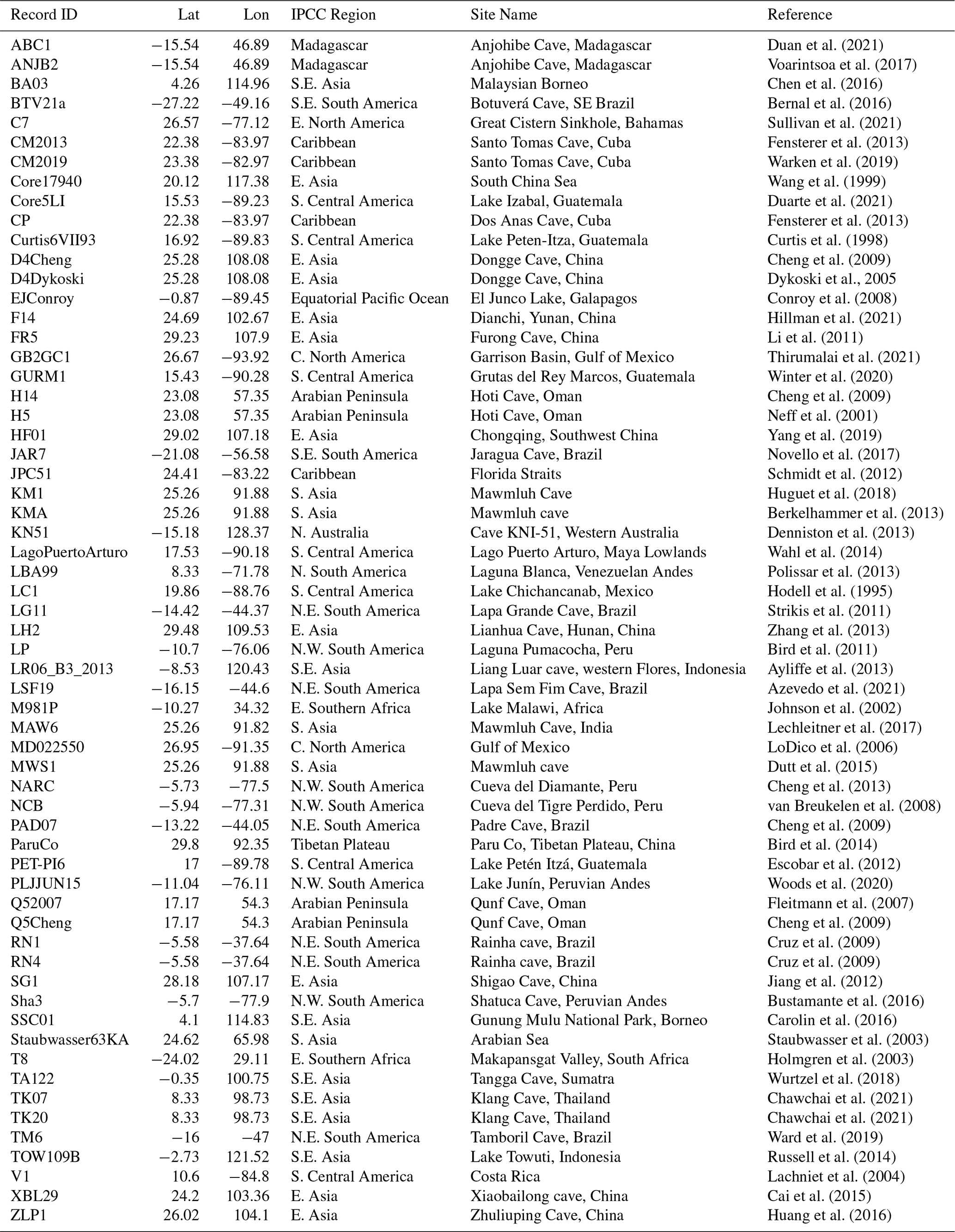
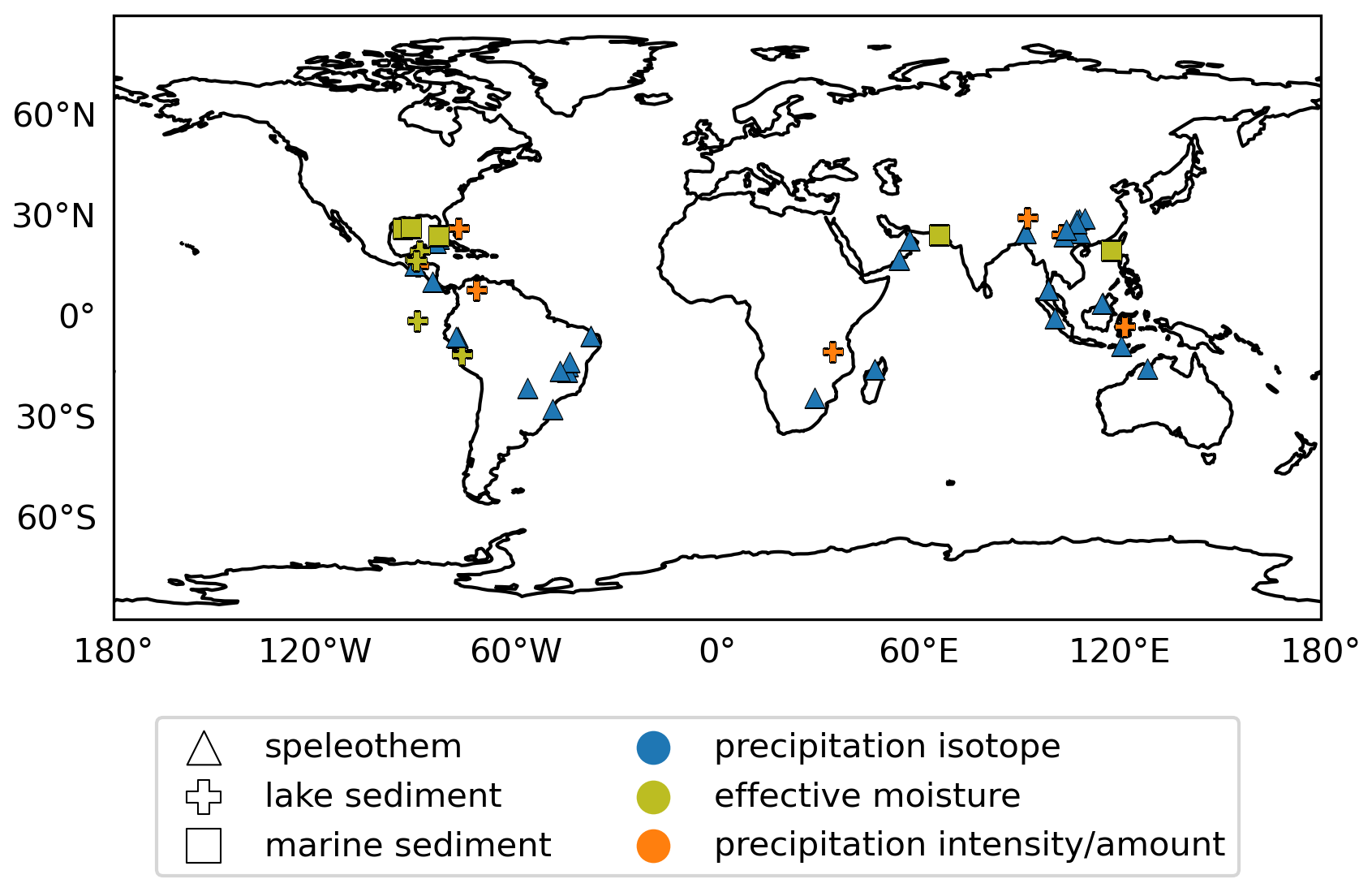
Figure 1 The location of the proxy records comprising each hydroclimate interpretation group included in this study.

The compilation was organized into three categories based on the climate interpretation of the various proxy records (Fig. 1): proxies which reflect the isotopic composition of precipitation (P_iso), proxies which reflect effective moisture (EM; P-E), and proxies which reflect precipitation amount and/or intensity (P_amt). This categorization scheme enables more robust interpretations of the proxy records and facilitates data-model comparison as our understanding of water isotopes and their manifestations in paleoclimate archives continues to advance (Konecky et al., 2020).

2.2 Age model development

Published radiometric age data were used to develop age-depth model ensembles for each dataset using Bayesian methods. Where available (Table A1), we employed age ensembles developed by the Past Global Changes (PAGES) Speleothem Isotope Synthesis and Analysis (SISAL) working group from version 2 of their database (Comas-Bru et al., 2020). For records for which these age ensembles were not available due to lack of inclusion in the SISALv2 database or comprising a lacustrine or marine sediment archive, we developed age-depth models using the geoChronR package (McKay et al., 2021) in R version 4.2.1 (R Core Team, 2021). All radiometric dates were obtained from the original publications and screened for updated age data where available. For records originating from the Northern Hemisphere tropics, radiometric dates were calibrated using the Northern Hemisphere calibration curve, IntCal20. Dates of records originating from the Southern Hemisphere tropics were calibrated using the Southern Hemisphere calibration curve, SHCal20. For each record, 1000 age-depth model iterations were run to generate a Markov Chain Monte Carlo (MCMC) age ensemble, which produces median age values and quantile age ranges, enabling the propagation of age-model uncertainties through subsequent analyses.

To reduce uncertainty arising from the differences in age modeling algorithms offered through geoChronR, we prioritized the use of BACON (Blaauw and Christen, 2011) across our records, including those in the SISALv2 database, where available. If a BACON age ensemble was not constructed for a SISALv2 dataset, we employed the Bchron (Haslett and Parnel, 2008) or copRA (Breitenbach et al., 2012) ensembles instead.

2.3 Detection of the 8.2 ka Event

Two event detection methods were used in this study, as detailed below. The start, end, and duration of hydroclimate anomalies associated with the 8.2 ka Event were calculated for all records where both methods detected events of the same sign. This was done to leverage the strengths of each detection method and provide a more robust reconstruction of the hydroclimate response to the 8.2 ka Event.

2.3.1 Modified Morrill method

For each record's published time series, we applied a modified version of the event detection methods described in Morrill et al. (2013) as a control for comparison with our actR results (hereafter referred to as MM; Fig. B1). Using 7.4–7.9 ka as a reference period, we calculate the mean and the standard deviation over that interval. From there, we define the upper and lower bounds by the two-sigma level. We repeat this process for a second reference period from 8.5–9.0 ka. We take the final upper and lower bounds as the most extreme values between the two reference periods. Then we use the 7.9–8.5 ka period as the 8.2 ka Event detection window.

Over this period, any values which exceed the upper or lower bound are marked as the 8.2 ka Event, with the timing of the event defined by the ages of the proxy values that exceed those bounds. For an excursion to be considered part of the 8.2 ka Event, the excursions must last at least 10 years. If multiple events are detected within the 7.9–8.5 ka window, they are combined into a single event if there are no more than three data points or thirty years separating the different excursions. This modification is necessary to account for the varying sampling resolutions present within and between several of the records in our compilation. If multiple events of differing signs are detected within the 8.2 ka Event window, the event with the largest z-score is chosen as the representative hydroclimate response. The magnitude of the event is defined by the largest absolute value z-score within the event detection period.

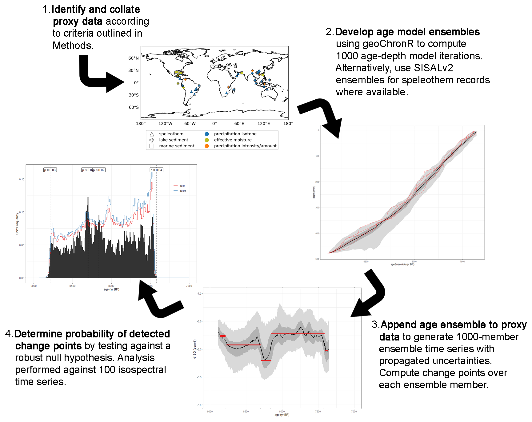
Figure 2 A schematic illustration of the actR analysis process. Step 1: Relevant records are identified and collated into our compilation based on the criteria outlined in the Methods (see Tables 1 and 2). Records are then converted to the LiPD file format for analysis. Step 2: A 1000-member age model ensemble is developed using geoChronR, or, where available for the speleothem records, drawn from the ensembles presented in version 2 of the SISAL database (Comas-Bru et al., 2020). This allows us to propagate age uncertainties through each successive analysis step. Step 3: The resulting 1000-member ensemble time series is then plotted, where at each time step, the median is represented by the black line, the outermost (lighter) bands represent extreme quantile values (0.025, 0.975) and the innermost (darker) bands the central quantile values (0.25, 0.75). The data are fit to a Gaussian distribution, and the change point analyses are conducted across this ensemble to determine the timing of change points in the proxy data. The red horizontal lines represent the mean proxy values calculated between those points. Step 4: The significance of the detected change points is tested by performing the same analyses against 100 isospectral surrogate time series, and the frequency of shifts is plotted as a black histogram summarized in 10-year-long bins. The 90 % and 95 % confidence intervals are plotted as red and blue lines, respectively, and the p-value is indicated when the frequency of shifts exceeds the 90 % confidence interval.

2.3.2 actR method

A second event detection method was used to account for age model uncertainties in the proxy records. Past studies (e.g., Morrill et al., 2013) employed statistical techniques to detect excursions in proxy records using the a priori assumption that the North Atlantic meltwater perturbation propagated globally at exactly 8.2 ka and lasted no more than 200 years. To better constrain the timing, duration, and magnitude of the 8.2 ka Event in this study, we employed an event detection algorithm based on the changepoint package in the newly developed Abrupt Change Toolkit in R (actR; McKay and Emile-Geay, 2022). This algorithm detects abrupt shifts in the mean of a time series based on a prescribed number of age model ensembles (generated in geoChronR), the minimum length of a segment (in years) over which mean shifts in the time series are detected, a user-defined changepoint detection method, and a weighting penalty function (Fig. 2). A minimum segment length of 50 or 100 years was assigned for each record in the proxy compilation to minimize short-lived transitions in the noisy proxy records, with the assumption that the 8.2 ka Event signal in each of the records lasts at least 50 years. For all but one record in our compilation, the 100-year minimum segment length optimally captured the major shifts in the data sets while minimizing the detection of spurious short-lived shifts. The exception was the speleothem record of Cheng et al. (2009; PAD07; Fig. C5), for which it was necessary to reduce the minimum segment length to 50 years to capture the clear isotopic depletion near 8.2 ka that was otherwise missed.

Detected changepoints were summarized over 10-year-long windows. The Pruned Exact Linear Time (PELT; Killick et al., 2012) changepoint detection method was chosen for its computational efficiency and dynamic programming approach to accurately identify the location and number of changepoints in time series data. The Modified Bayesian Information Criterion (MBIC; Zhang and Siegmund, 2007) was chosen as the penalty weighting function to balance the goodness of fit of the model to the data with the complexity of the model and the number of changepoints. These methods effectively minimize the detection of spurious changepoints within each ensemble. Each time series ensemble was tested against a robust null hypothesis using surrogate proxy data generated by an isospectral noise model. By construction, the surrogate data have the same power spectrum as the original data, but phase scrambling destroys any autocorrelation that was present in the original time series. If autocorrelation is detected in a segment of the original time series ensemble, it fails the null hypothesis test, and any changepoint detected within that segment is excluded from the result. This test helps to ensure that the detected changepoints are statistically significant and not just the result of random variation. Both age and proxy data uncertainties are propagated through each ensemble, improving the robustness of the result. For each record, 1000 age model ensembles were generated and tested against 100 surrogate time series.

The actR event detection algorithm can be compromised by variable sampling resolution. Therefore, for records with highly variable resolution, we used the MM method to determine event onset, termination, and duration. This applies to only two records: the speleothem record from Dykoski et al. (2005; D4Dykoski, Fig. C7) and the speleothem record from Neff et al. (2001; H5; Fig. C10).

Two types of events were characterized based on the actR results. “Significant events” are defined by the presence of two consecutive changepoints with p<0.05 over the 7.9–8.3 ka window (“start” and “end”. If more than two consecutive changepoints exist over that window, the two with the lowest p-values and highest probability are used. The difference between “start” and “end” dates is used to calculate event duration, which we assume to be between a minimum of 20 and a maximum of 300 years. The magnitude of “events” is determined by the greatest absolute value z-score in each record's median age ensemble time series between the actR-derived “start” and “end” dates, with interpretation based on the sign of the z-score corresponding to the interpretation direction of the original authors. “Tentative events” are defined by the presence of two consecutive changepoints with p<0.1 over an extended 7.7–8.5 ka window. Events lasting more than 300 years are removed from consideration. If more than two events are detected within that window, the event with the start date closer to 8.2 ka is chosen as the final 8.2 ka Event.

2.4 iCESM simulations

The National Center for Atmospheric Research's (NCAR) water isotope-enabled Community Earth System Model (iCESM1.2; Brady et al., 2019) is a state-of-the-art, fully coupled GCM designed to simulate water isotopes across all stages of the global hydroclimate cycle. It employs the CAM5.3 atmospheric model, with a gridded resolution of 1.9° latitude × 2.5° longitude and 29 vertical levels. Land processes are modeled by CLM4, at the same nominal 2° resolution. CLM is coupled to a River Transport Model which routes runoff from the land into oceans and/or marginal seas. Both the POP2 ocean model and the CICE sea ice model have a common grid size of 320 × 384 with a nominal 1° resolution near the equator and in the North Atlantic. While iCESM faithfully captures the broad quantitative and qualitative features of precipitation isotopes, it is known to have a global bias toward depleted precipitation δ¹⁸O (δ¹⁸O_p; median bias of −2.5 ‰; Brady et al., 2019).

We performed a new 8.2 ka Event meltwater-forced (“hosing”) simulation and an early Holocene control simulation (“ctrl”) using iCESM1.2. iCESM enables explicit tracking of water isotopes throughout the global water cycle, facilitating quantitative comparisons between model output and water isotope-based proxy records. These simulations followed the Paleoclimate Modeling Intercomparison Project 4-Coupled Model Intercomparison Project 6 (PMIP4-CMIP6) 8.2 ka simulation parameters (Otto-Bliesner et al., 2017), with two exceptions. Firstly, the freshwater flux was applied across the entire northern North Atlantic in our simulations (instead of just in the Labrador Sea as in PMIP4). While this method is expected to overestimate the subsequent AMOC and climate response to the 8.2 ka Event, it eliminates the sensitivity to poorly resolved deepwater formation regions in the model. We thus focus on the patterns of the tropical rainfall response to an abrupt AMOC weakening, rather than the magnitude of the response. Secondly, our hosing experiment branches from 9 ka boundary conditions (instead of 9.5 ka as in PMIP4), and thus uses slightly different orbital and GHG configurations from PMIP4. However, the impact of these marginally different boundary conditions is expected to be minimal.

For the 9 ka control simulation, the model was forced with prescribed greenhouse gas concentrations (CH₄=658.5 ppb, CO₂=260.2 ppm, and N₂O =255 ppb), orbital configurations (eccentricity =0.019524°, obliquity =24.2030°, and longitude of perihelion =99.228°), and a reconstruction of the ice sheet extent (Peltier et al., 2015) representative of conditions at 9 ka. The orbital configuration is characterized by larger obliquity, slightly higher eccentricity, and a change in the longitude of perihelion relative to present day that resulted in increased seasonality of insolation in the Northern Hemisphere (Wu et al., 2018; Hu et al., 2019). These factors produced warmer Northern Hemisphere summers, especially in mid to high latitudes, which promoted the retreat of the remnant Laurentide Ice Sheet (LIS) (Otto-Bliesner et al., 2017 and references therein). The control simulation (“ctrl”) was initialized from an earlier 400-year-long 9 ka simulation and run for 100 model years using these parameters.

The 8.2 ka Event simulation (“hose”) was branched from year 100 of the 9 ka control run. Initially, a simulated 2.5 Sv meltwater flux (meltwater δ¹⁸O $=-\mathrm{30}\mathrm{‰}$; Zhu et al., 2017) was applied across the northern North Atlantic Ocean (50–70° N) for 1 year, followed by 0.13 Sv flux for 99 years to approximate the abrupt drainage of Lakes Agassiz and Ojibway and eventual collapse of the LIS at Hudson Bay (Otto-Bliesner et al., 2017). Monthly surface air temperature, precipitation amount, and δ¹⁸O_p variables were extracted from each simulation for analysis. To isolate the global response to the simulated 8.2 ka Event, yearly time series of temperature (°C), precipitation amount (mm d⁻¹), and amount-weighted δ¹⁸O_p (‰) were obtained. Anomalies for each variable were calculated by subtracting the final 50 years of the “ctrl” simulation from the final 50 years of the “hose” simulation.

2.5 Decomposition of changes in precipitation δ¹⁸O

The difference in amount-weighted δ¹⁸O_p between the hosing and control simulations is:

$$\begin{array}{}\text{(1)}& {{\mathit{\delta }}^{\mathrm{18}}\mathrm{O}}_{\mathrm{p},\mathrm{hose}}-{{\mathit{\delta }}^{\mathrm{18}}\mathrm{O}}_{\mathrm{p},\mathrm{ctrl}}={\displaystyle \frac{\sum _j{{\mathit{\delta }}^{\mathrm{18}}\mathrm{O}}_{j,\mathrm{hose}}{P}_{j,\mathrm{hose}}}{\sum _j{P}_{j,\mathrm{hose}}}}-{\displaystyle \frac{\sum _j{{\mathit{\delta }}^{\mathrm{18}}\mathrm{O}}_{j,\mathrm{ctrl}}{P}_{j,\mathrm{ctrl}}}{\sum _j{P}_{j,\mathrm{ctrl}}}}\end{array}$$

where δ¹⁸O_j is the monthly isotopic composition of precipitation and P_j is the monthly precipitation rate (in mm d⁻¹), for each month in the simulation period. This change in amount-weighted δ¹⁸O_p can arise from both local and nonlocal processes. Following Liu and Battisti (2015), the change in amount-weighted δ¹⁸O_p is decomposed into two components: (i) those resulting from changes in the amount of monthly precipitation and (ii) those resulting from changes in the monthly isotopic composition of precipitation. The latter component may be due to changes in local precipitation intensity and/or to changes in the isotopic composition of the water vapor which forms the condensate. The importance of changes in the amount of monthly precipitation (i.e. precipitation seasonality) to changes in δ¹⁸O_p is given by:

$$\begin{array}{}\text{(2)}& {\displaystyle \frac{{\sum }_j{{\mathit{\delta }}^{\mathrm{18}}\mathrm{O}}_{j,\mathrm{ctrl}}{P}_{j,\mathrm{hose}}}{\sum _j{P}_{j,\mathrm{hose}}}}-{\displaystyle \frac{\sum _j{{\mathit{\delta }}^{\mathrm{18}}\mathrm{O}}_{j,\mathrm{ctrl}}{P}_{j,\mathrm{ctrl}}}{\sum _j{P}_{j,\mathrm{ctrl}}}}\end{array}$$

and the importance of changes in the monthly isotopic composition of precipitation to changes in δ¹⁸O_p is given by:

$$\begin{array}{}\text{(3)}& {\displaystyle \frac{\sum _j{{\mathit{\delta }}^{\mathrm{18}}\mathrm{O}}_{j,\mathrm{hose}}{P}_{j,\mathrm{ctrl}}}{\sum _j{P}_{j,\mathrm{ctrl}}}}-{\displaystyle \frac{\sum _j{{\mathit{\delta }}^{\mathrm{18}}\mathrm{O}}_{j,\mathrm{ctrl}}{P}_{j,\mathrm{ctrl}}}{\sum _j{P}_{j,\mathrm{ctrl}}}}\end{array}$$

Note that Eqs. (2) and (3) do not sum to the total change in δ¹⁸O_p due to nonlinearity in the definition of δ¹⁸O_p.

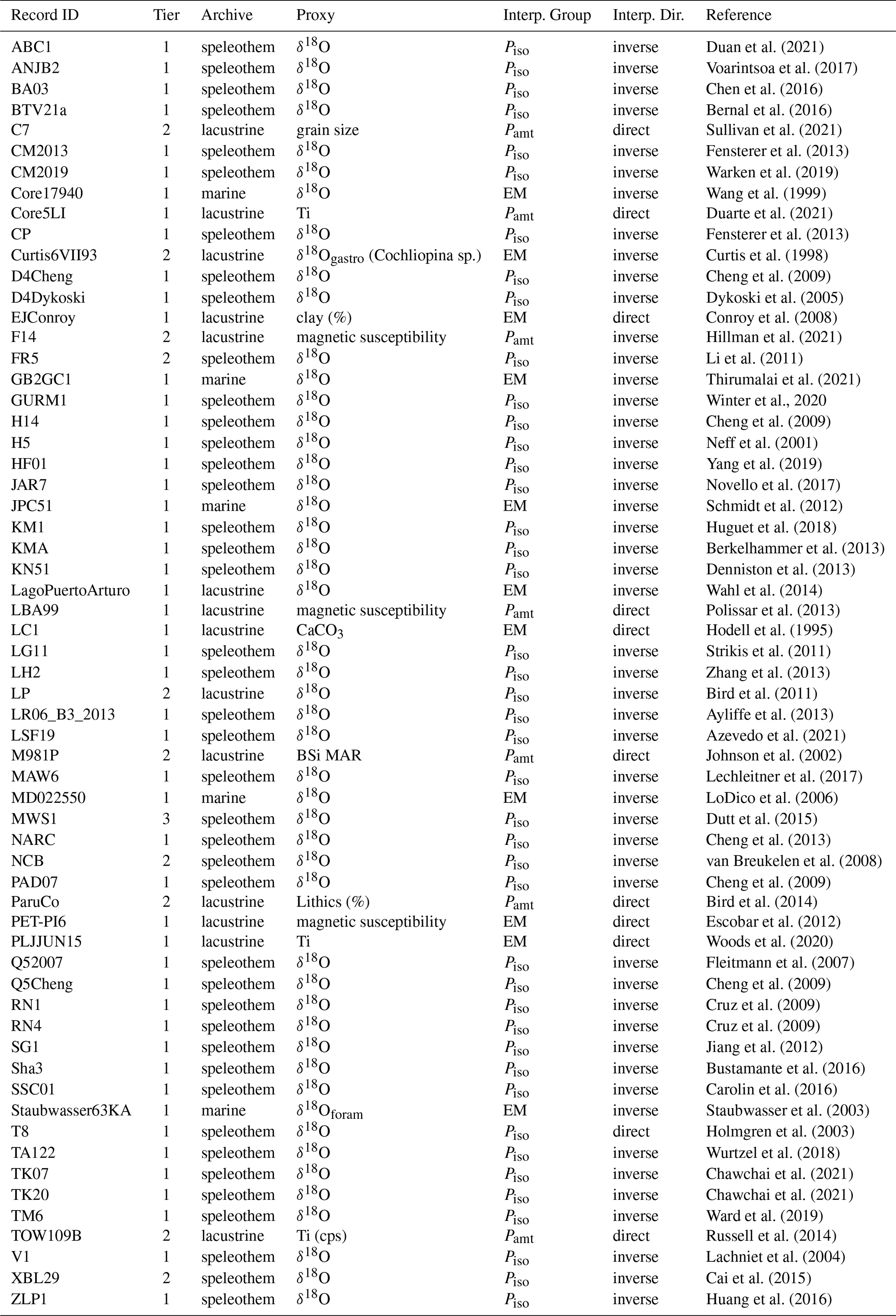
Table 2 Archive and interpretation metadata for the paleoclimate proxy datasets used in this study. Tier 1 data meet all strict inclusion criteria, while Tier 2 data are deficient in either dating or data resolution over the 7–10 ka interval. Tier 3 data meet none of the strict inclusion criteria and are not included in quantitative analyses. All foraminifera used in the compilation are G. ruber (white). BSi MAR is the biogenic silica mass accumulation rate, in mg SiO₂ cm⁻² yr⁻¹.

3 Results

3.1 Data compilation

This study compiled 61 tropical hydroclimate proxy records covering 17 IPCC-designated climate regions (Fig. B2; Iturbide et al., 2020). Compared to Morrill et al. (2013), our compilation substantially improves hydroclimate proxy data coverage across the Caribbean, Central America, South America, South and East Asia, and the Maritime Continent. The compilation comprises 42 speleothem records (∼ 69 %), 14 lacustrine records (∼ 23 %), and 5 marine records (∼ 8 %; Table 2). When categorized by hydroclimate interpretation, the compilation includes 43 P_iso records (70.5 %), 11 EM records (18 %), and 7 P_amt records (11.5 %; Fig. 1; Table 2). For the purpose of this study, records which fully meet all inclusion criteria are designated as Tier 1 records (n=50, 82 %), forming the basis for the data-model intercomparison. Records which fail to meet either the minimum paleodata resolution or radiometric date requirements are classified as Tier 2 records and are included as supporting datasets (n=10, 16 %). One record (MWS1; Dutt et al., 2015) failed to meet both requirements, thus it is designated as a Tier 3 record, and has been excluded from further analysis.

3.2 Timing, magnitude, and duration of the 8.2 ka Event in the proxy compilation

The approximate start, end, and duration of hydroclimate anomalies associated with the 8.2 ka event were calculated for all records where both our MM and actR event detection methods detected events of the same sign (wetter, drier, or no change). This approach provides a more robust reconstruction of the hydroclimate response to the 8.2 ka Event than either method would achieve in isolation. 30 of the 61 records (49 %) in our compilation exhibited such agreement between the two detection methods. The remaining 31 records displayed disagreement between the two detection methods and were thus excluded from further analysis.

Of the 30 records that exhibit agreement between the two detection methods, significant hydroclimate events were detected in 18 records (34 % of all Tier 1 and 10 % of all Tier 2 records), with the remaining 12 records showing no event in either detection method (14 % of all Tier 1 records and 50 % of all Tier 2 records). The lower event detection frequency in Tier 2 compared to Tier 1 records highlights the importance of using high resolution records with good age constraints for the detection of abrupt climate events, as the threshold for event detection is rarely exceeded in records that are low resolution and/or have large age uncertainty (i.e., Tier 2 records).

Globally, detected hydroclimate anomalies had average onset at 8.28 ka, average termination at 8.13 ka, and average duration of 152 years. The longest events occurred in the Gulf of Mexico sedimentary foraminifera δ¹⁸O record (LoDico et al., 2006; MD022550; Fig. C4; 289 years) and the Chongqing, China speleothem record (Yang et al., 2019; HF01; Fig. C11; 259 years). The Chinese lacustrine magnetic susceptibility record of Hillman et al. (2021; F14; Fig. C8) has the earliest event onset age of 8.49 ka, with a termination at 8.34 ka, for a total duration of 152 years, while the Chinese speleothem record of Dykoski et al. (2005; D4Dykoski; Fig. C7) has the latest event onset age at roughly 8.11 ka, terminating near 8.04 ka, for an event duration of 62 years.

In the final set of 30 records (that agree on the sign of the event between the MM and actR methods), drier and/or isotopically enriched events were detected in 13 of those 30 records (Table 5), including six records from East Asia (Fig. 5), with the largest events (+3.0σ, +5.8σ) detected in the speleothem record of Yang et al. (2019; HF01; Fig. C11) and the magnetic susceptibility record of Hillman et al. (2021; F14; Fig. C8). Similarly, drying/isotopic enrichment was seen in three speleothem records from the Arabian Peninsula, with the largest event (+3.5σ) detected in the record of Cheng et al. (2009; H14; Fig. C9) between 8.08 and 8.21 ka. The two speleothem records of Chawchai et al. (2021) from Klang Cave, Thailand (TK07, Fig. C15; TK20, Fig. C16) showed similarly high levels of isotopic enrichment (+3.1σ and +2.5σ) between approximately 8.16 and 8.30 ka. Two large drying/enrichment events were also detected in central America, including a positive isotopic excursion of +3.4σ in the Costa Rican speleothem record of Lachniet et al. (2004; V1; Fig. C17) from 8.05 and 8.19 ka and a negative excursion (−4.0σ) in titanium content (indicative of a drying event) in the Guatemalan lake sediment record of Duarte et al. (2021; Core5LI; Fig. C6) from 8.09 and 8.16 ka, suggesting a regional hydroclimate response to the 8.2 ka Event in southern Central America, south of the Yucatan Peninsula (Fig. 7).

Wetter and/or isotopically depleted events were detected in five of the 30 records in the final compilation. Namely, the Madagascar speleothem records of Voarintsoa et al. (2017; ANJB2; Fig. C2) and Duan et al. (2021; ABC1; Fig. C1) showed negative isotopic excursions of −3.0σ and −2.5σ, respectively, while the two Brazilian speleothem records from Lapa Grande Cave (Strikis et al., 2011; LG11; Fig. C3) and Padre Cave (Cheng et al., 2009; PAD07; Fig. C5) exhibited negative isotopic excursions of −2.9σ and −2.7σ, respectively (Table 5). In addition, a large isotopic depletion event (−3.8σ) was detected in the foraminifera δ¹⁸O record from the Gulf of Mexico (LoDico et al., 2006; MD022550; Fig. C4).

We found no significant hydroclimate response in the remaining 12 records of our compilation, with both the MM and actR event detection methods in agreement that no event occurred. This category included three lake sediment records from the Yucatan Peninsula (Figs. 7c and B7c; LC1, Hodell et al., 1995; Fig. C25, Curtis6VII93, Curtis et al., 1998; Fig. C20, LagoPuertoArturo, Wahl et al., 2014; Fig. C24), two speleothem records from Southeast Asia/the Maritime Continent (Figs. 8 and B8; KMA, Berkelhammer et al., 2013; Fig. C23, SSC01, Carolin et al., 2016; Fig. C29), and two speleothem records from Brazil (Figs. 6 and B6; RN1, Cruz et al., 2009; Fig. C28, TM6, Ward et al., 2019; Fig. C30).

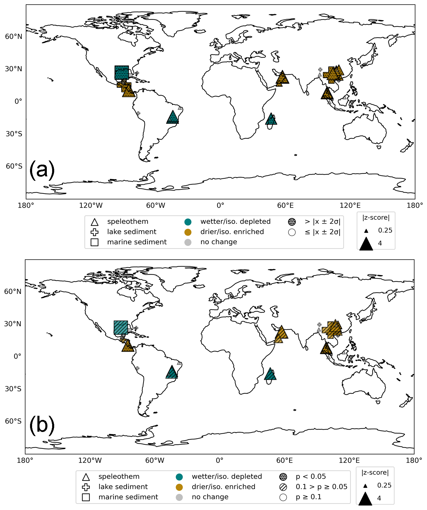
Figure 3 (a) Map of the detected 8.2 ka hydroclimate events using the modified Morrill et al. (2013) method (MM). Blue symbols represent wetter (and/or isotopically depleted) conditions while brown symbols represent drier (and/or isotopically enriched) conditions. Grey symbols indicate the locations of proxy data where no significant change was detected. Archive type is indicated by the symbol shape, and symbol size is scaled by $\mathrm{250}\ln (\mathrm{1}+|z\text{-score}\left|\right)$, calculated from the per-record mean and standard deviation over the 7–10 ka interval. Stippling indicates an event detected over the 7.9–8.5 ka detection window. (b) Same as for (a) but using the actR event detection method. Here, stippling indicates that a “significant” event was detected in each record by actR with event “start” and “end” times within the 7.9–8.3 ka interval at the p<0.05 significance level. Slashed hatching indicates the presence of a “tentative” hydroclimate anomaly, defined by two consecutive changepoints with p<0.1 over an extended 7.7–8.5 ka window (see Methods).

3.3 Regional coherency of the reconstructed hydroclimate changes

The spatial pattern of reconstructed hydroclimate anomalies shows substantial regional coherency (Fig. 3), though it does not strictly conform to the hemispheric dipole pattern associated with the 8.2 ka Event (i.e., a generally drier/isotopically enriched Northern Hemisphere and wetter/isotopically depleted Southern Hemisphere). Both the MM and actR event detection methods indicate prominent drying/enrichment across East and Southeast Asia, as well as the Arabian Peninsula. These dry conditions are interspersed with areas of no change in parts of the Maritime Continent and eastern India/Tibetan Plateau. No robust signatures of the 8.2 ka Event are observed over the Maritime Continent. Central and South America display more of a hemispheric dipole pattern, with dry/enrichment events occurring north of the equator in Costa Rica and Guatemala, contrasting with wet/depletion events south of the equator in eastern Brazil. However, there are also regions in northern and central Brazil that exhibit no hydroclimate response. The proxy records thus present a far more complex, regionally specific hydroclimate response to the 8.2 ka Event than a simple hemispheric dipole pattern.

In several regions (including East Asia, Fig. 5; and northeastern South America, Fig. 6), records with no detected change are located near records with clear event signals. These regional differences could arise from several factors, including localized hydroclimate responses to the event, age uncertainty, and proxy interpretation uncertainties. For example, speleothem δ¹⁸O records have been interpreted as representing a range of different climate processes, often within the same region, including changes in regional precipitation amount, monsoon strength, moisture source location, upstream rainout, seasonal frontal shifts, and temperature (e.g. Hu et al., 2019), reflecting the complexity of processes that impact δ¹⁸O_p and speleothem δ¹⁸O. Because of the inherently regional nature of rainfall patterns and the uncertainties in the proxy records, we focus our interpretation on regional hydroclimate signals that are supported by multiple records, often across different aspects of hydroclimate. In this way, we focus on the most robust aspects of the tropical hydroclimate response to the 8.2 ka Event.

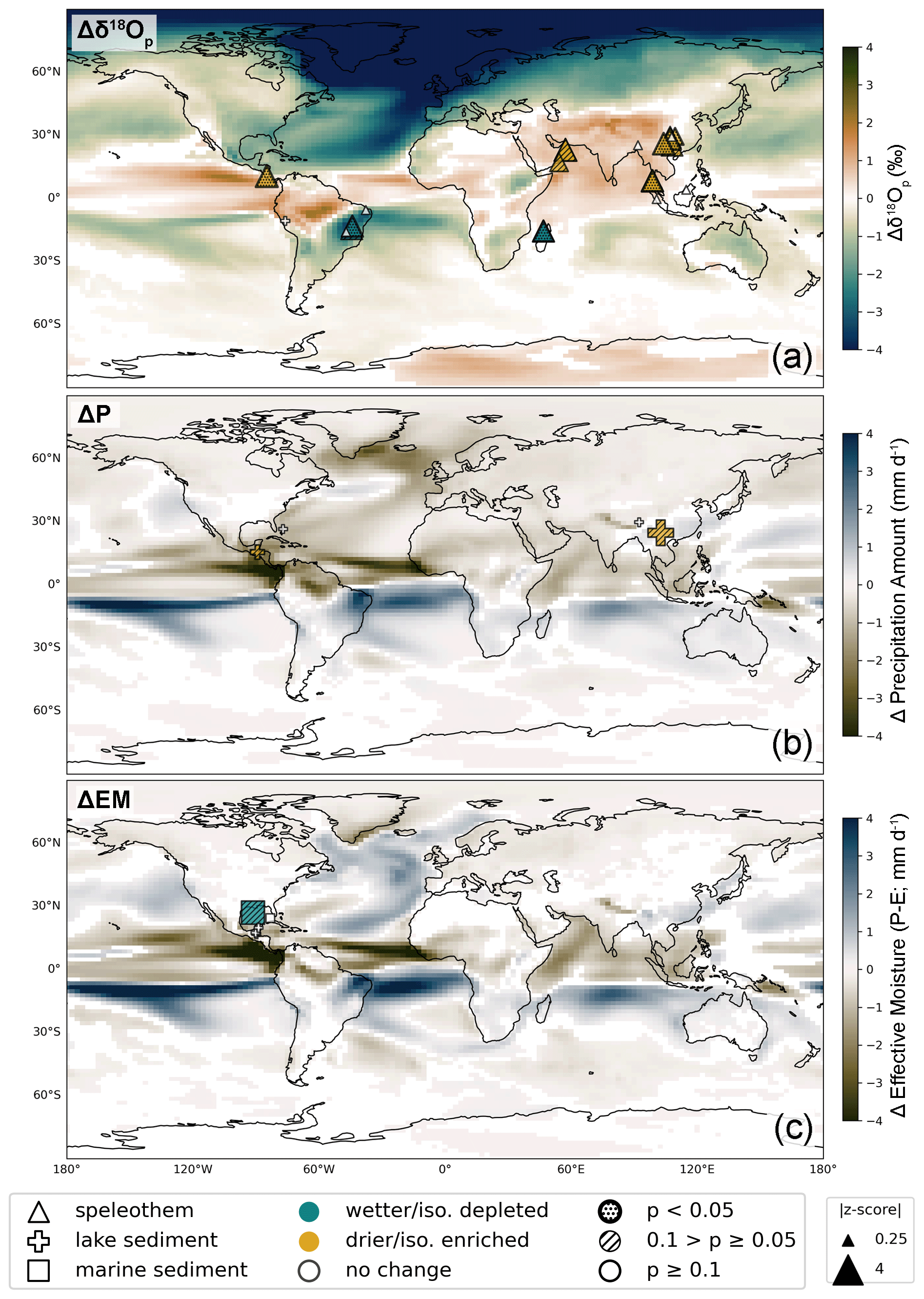
Figure 4 Proxy symbols from Fig. 3b overlaid on contour maps of the simulated anomalous (a) amount-weighted δ¹⁸O_p, (b) precipitation amount, and (c) effective moisture (P-E), calculated from the difference between the last 50 years of the iCESM “hose” and “ctrl” experiments, where only anomalies that exceed the 95 % confidence level (p<0.05) are plotted.

3.4 Global signature of the 8.2 ka Event in iCESM

We now compare these reconstructed hydroclimate patterns to those simulated by iCESM under meltwater forcing. Within 20–30 years after the hosing is initiated, the AMOC weakens to roughly 20 % of its original strength. The surface temperature response in iCESM exhibits the characteristic “bipolar seesaw” pattern (i.e., a colder northern hemisphere and warmer southern hemisphere, most pronounced in the Atlantic Ocean), consistent with reduced northward heat transport by AMOC (Fig. B3). Anomalously cool surface temperatures, reaching as low as −20 °C where the freshwater forcing was applied, stretch across the northern North Atlantic Ocean, southward along the western coasts of Europe and North Africa, and into the tropical Atlantic via the North Atlantic Subtropical Gyre. Surface air temperatures across the Southern Hemisphere show a positive anomaly of up to 3 °C, with the largest warming occurring in the South Atlantic. Over the continents, surface air temperatures cool in all regions except localized parts of northern South America, West Africa, and the southernmost regions of South America and Australia.

Accompanying these temperature anomalies are notable anomalies in precipitation amount, δ¹⁸O_p, and effective moisture (Fig. 4). Precipitation decreases while effective moisture increases throughout much of the North Atlantic, with the responses most pronounced in the regions with greatest cooling. The increase in effective moisture in this region indicates that the evaporation reduction outpaces the precipitation reduction (Fig. 4c). Large scale drying occurs across much of the northern tropics, with the largest precipitation anomalies occurring in the tropical Pacific and Atlantic basins associated, with a southward shift of the Pacific and Atlantic ITCZs occurring in response to the freshwater forcing (Fig. 4b). These shifts are characterized by a weakening of the northern extent of the ITCZs and an enhancement of the southern extent. A notable hemispheric dry/wet dipole pattern is occurs in the central/eastern tropical Pacific and tropical Atlantic, extending over northeastern South America. This pattern is less pronounced but still present over the tropical Indian Ocean and Africa. In contrast, no such dipole occurs over the western Pacific or Maritime Continent. Notably, the simulated pattern in δ¹⁸O_p in iCESM under meltwater forcing is remarkably similar to that in GISS ModelE-R (Fig. 4a; Lewis et al., 2010), indicating a robust inter-model response in δ¹⁸O_p to North Atlantic meltwater forcing (aside from Africa and Antarctica, where the inter-model agreement breaks down).

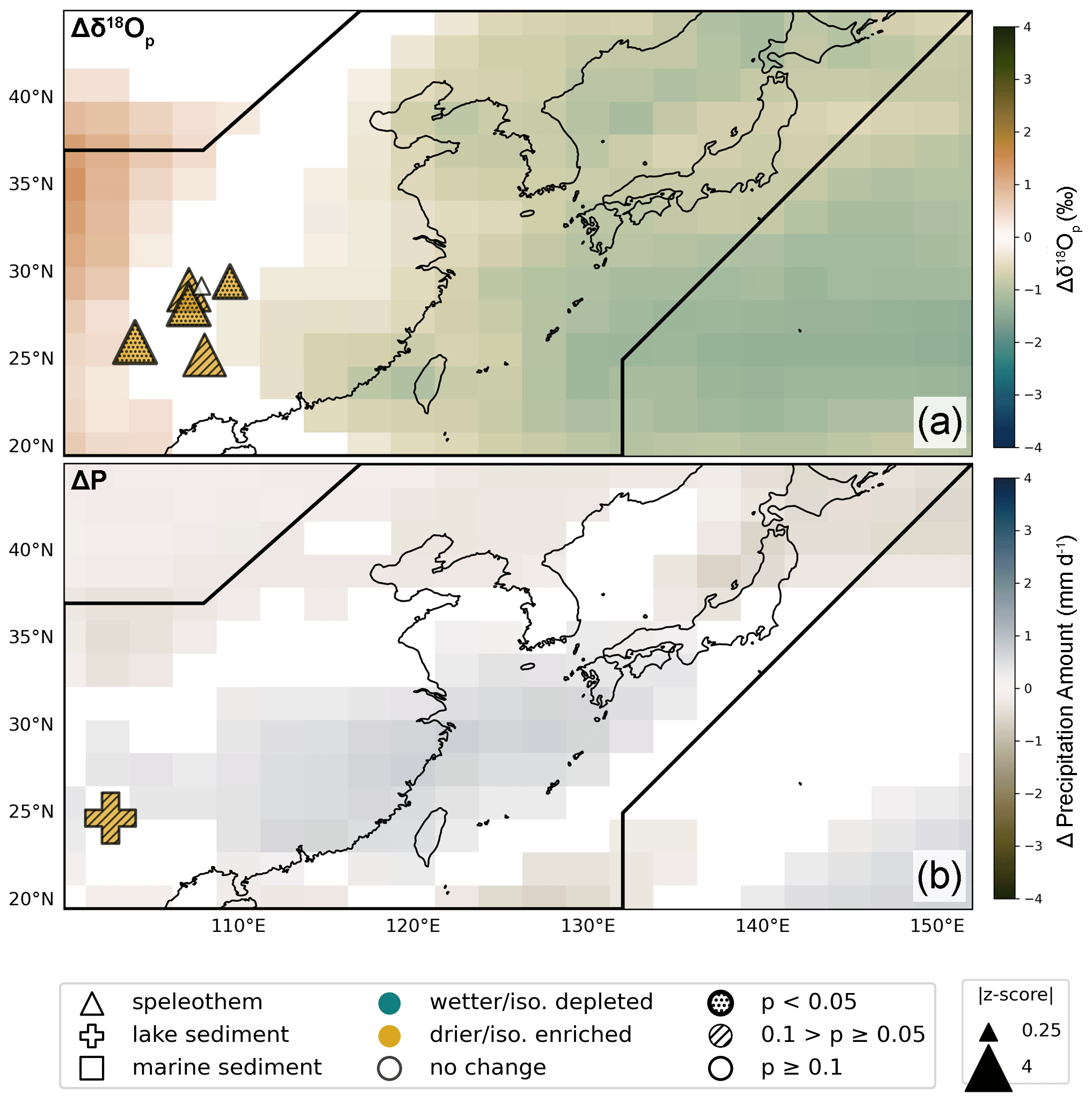
Figure 5 Data-model comparison of IPCC region 35: East Asia (box). Model shading represents (a) the amount-weighted δ¹⁸O_p anomaly, and (b) the precipitation amount anomaly between the last 50 years of the “hose” and “ctrl” simulations that exceed the 95 % confidence level (p<0.05) using an unpaired two sample Student's t-test. Symbols represent paleoclimate proxy archives within the region corresponding to each respective climate variable, where the brown shaded triangles indicate speleothem records with recorded dry hydroclimate/enriched isotopic anomalies during the 8.2 ka Event and grey symbols indicate records with no hydroclimate anomalies (“no change”) over the 7.9–8.3 ka interval. For symbols showing an anomaly associated with the 8.2 ka Event, size is scaled by $\mathrm{400}\ln (\mathrm{1}+|z\text{-score}\left|\right)$ relative to each record's mean and standard deviation.

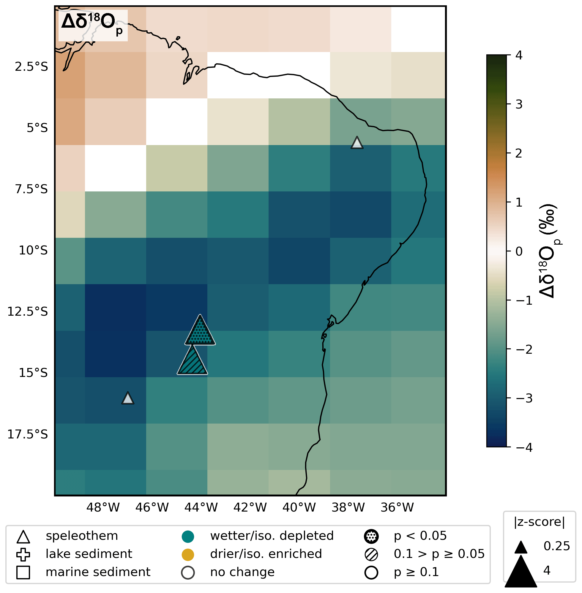
Figure 6 As in Fig. 5, but for IPCC region 11: northeastern South America (box). Model shading represents the amount-weighted δ¹⁸O_p anomaly between the last 50 years of the “hose” and “ctrl” simulations.

These temperature and precipitation anomalies project strongly onto the amount-weighted δ¹⁸O_p values (Fig. 4a). The greatest δ¹⁸O_p anomalies occur in the northern reaches of the North Atlantic Ocean, reaching up to −8 ‰ in association with the strong regional cooling of the North Atlantic, as well as the addition of highly depleted (−30 ‰) meltwater to the surface ocean of the “hosing” site, and subsequent evaporation and rainout. In the tropics, δ¹⁸O_p anomalies closely follow the changes in precipitation amount over the equatorial Atlantic and central/eastern Pacific Oceans, with negative δ¹⁸O_p anomalies south of the equator and positive δ¹⁸O_p anomalies north of the equator. A pronounced dipole pattern is also evident over northern South America, where increased (decreased) rainfall corresponds to negative (positive) δ¹⁸O_p anomalies in the southeastern (northwestern) region of South America. In the tropical Atlantic and Central America, a second dipole in δ¹⁸O_p occurs ∼ 12° N, with isotopic enrichment south of this latitude, extending over Panama and Costa Rica, following the largescale drying pattern, but isotopic depletion north of this latitude, including over the remainder of Central America, associated with the upwind cooling of SSTs and the addition of isotopically depleted meltwater to the North Atlantic. In the Middle East, India, Tibetan Plateau, and parts of Southeast Asia, modest drying is accompanied by pronounced positive δ¹⁸O_p anomalies. There appears to be no clear relationship between precipitation amount and δ¹⁸O_p anomalies over Africa, East Asia, the Western Pacific, and Maritime Continent.

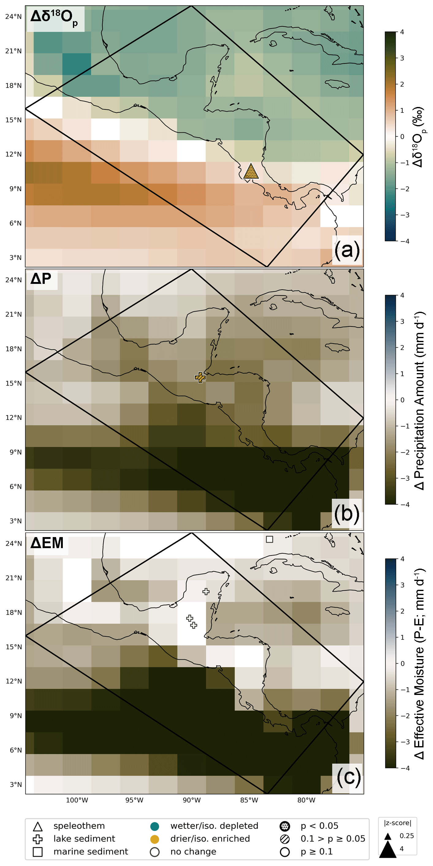
Figure 7 As in Fig. 5, but for IPCC region 7: southern Central America (box), with the addition of (c) the effective moisture (precipitation minus evaporation) anomaly between the last 50 years of the “hose” and “ctrl” simulations.

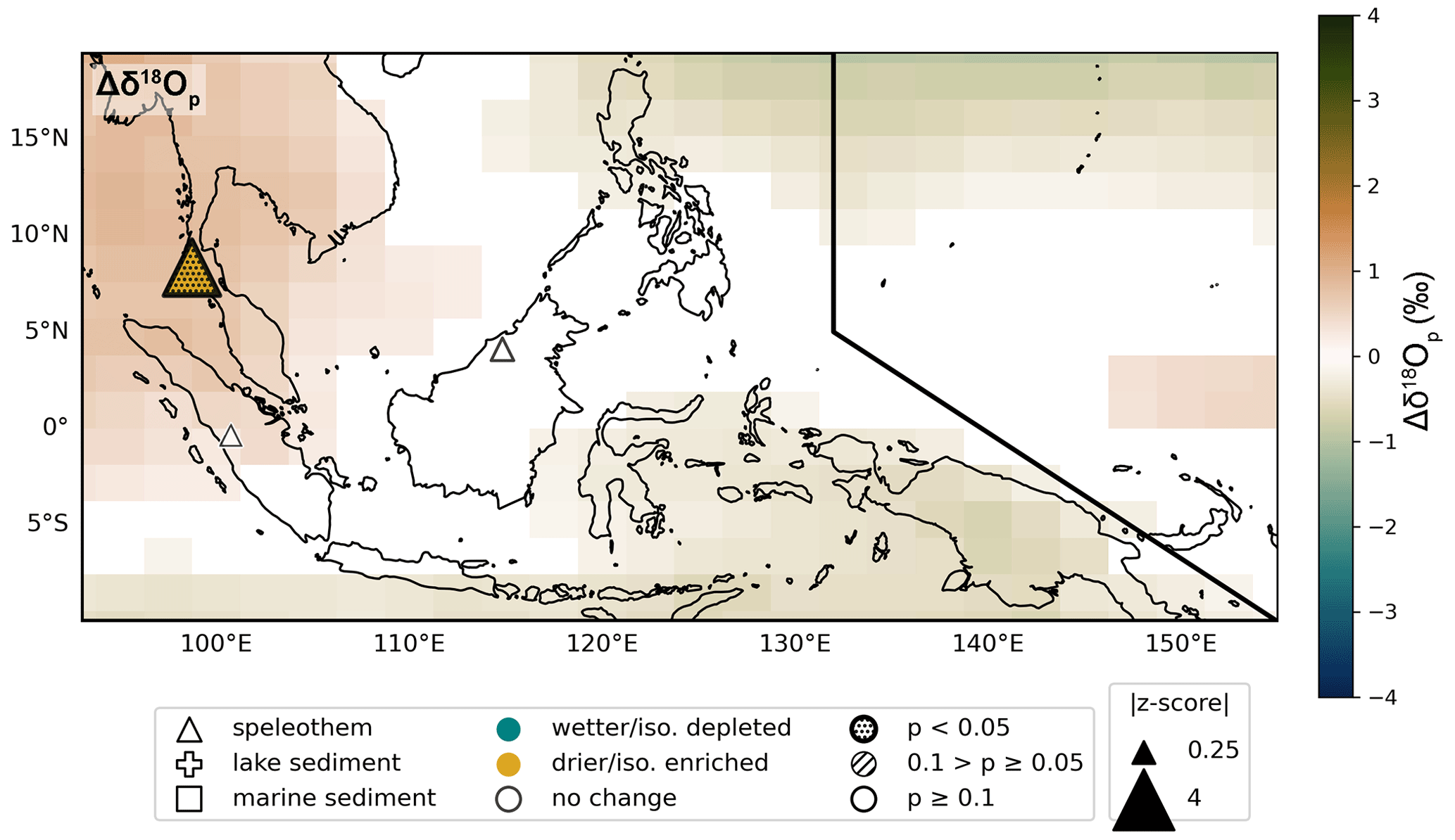
Figure 8 As in Fig. 5, but for IPCC region 38: Southeast Asia (box). Model shading represents the amount-weighted δ¹⁸O_p anomaly between the last 50 years of the “hose” and “ctrl” simulations.

3.4.1 Mechanisms driving the response of precipitation δ¹⁸O to North Atlantic freshwater forcing

To assess whether the simulated hydroclimate changes are due to changes in δ¹⁸O_p or changes in the seasonality of precipitation, we decomposed the changes in amount-weighted δ¹⁸O_p following Liu and Battisti (2015; Fig. 9). In East Asia, the change in amount-weighted δ¹⁸O_p, including the east-west dipole pattern with isotopic depletion off the coast of China into the North Pacific and isotopic enrichment inland, is driven by changes in δ¹⁸O_p (Fig. 10b, c). Under meltwater forcing, δ¹⁸O_p inland is more enriched throughout the year, particularly in the dry season from December to April (Fig. 12c). While δ¹⁸O_p off the coast is more depleted throughout the year, particularly during the wet season from June to November (Fig. 12d). Consistent with previous studies on Heinrich events, these results suggest that the meltwater-induced enrichment in Chinese speleothem δ¹⁸O records is not driven by changes in local precipitation and/or the strength of the EASM, but rather driven by changes in moisture source, circulation, and/or upstream rainout (Chiang et al., 2020; Pausata et al., 2011, Lewis et al., 2010). That the largest changes in δ¹⁸O_p over China occur during the winter season is consistent with the results from Lewis et al. (2010), which found that increased moisture provenance in the Bay of Bengal during winter yielded enriched δ¹⁸O_p over China during Heinrich events. The large zonal asymmetry observed in the δ¹⁸O_p response to meltwater forcing between China and the North Atlantic was also identified in the Heinrich simulations of Lewis et al. (2010) and Pausata et al. (2011).

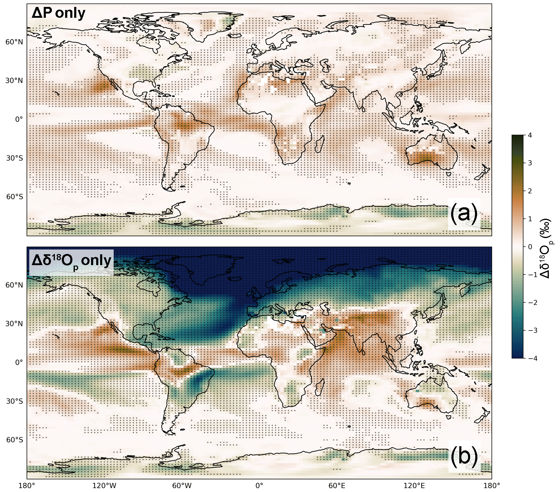
Figure 9 The contribution of (a) the changes in the amount of monthly precipitation and (b) the monthly changes in δ¹⁸O_p to the total change in mean annual amount-weighted δ¹⁸O_p between the last 50 years of the “hose” and “ctrl” simulations. Stippling represents data plotted at the 95 % confidence level (p<0.05).

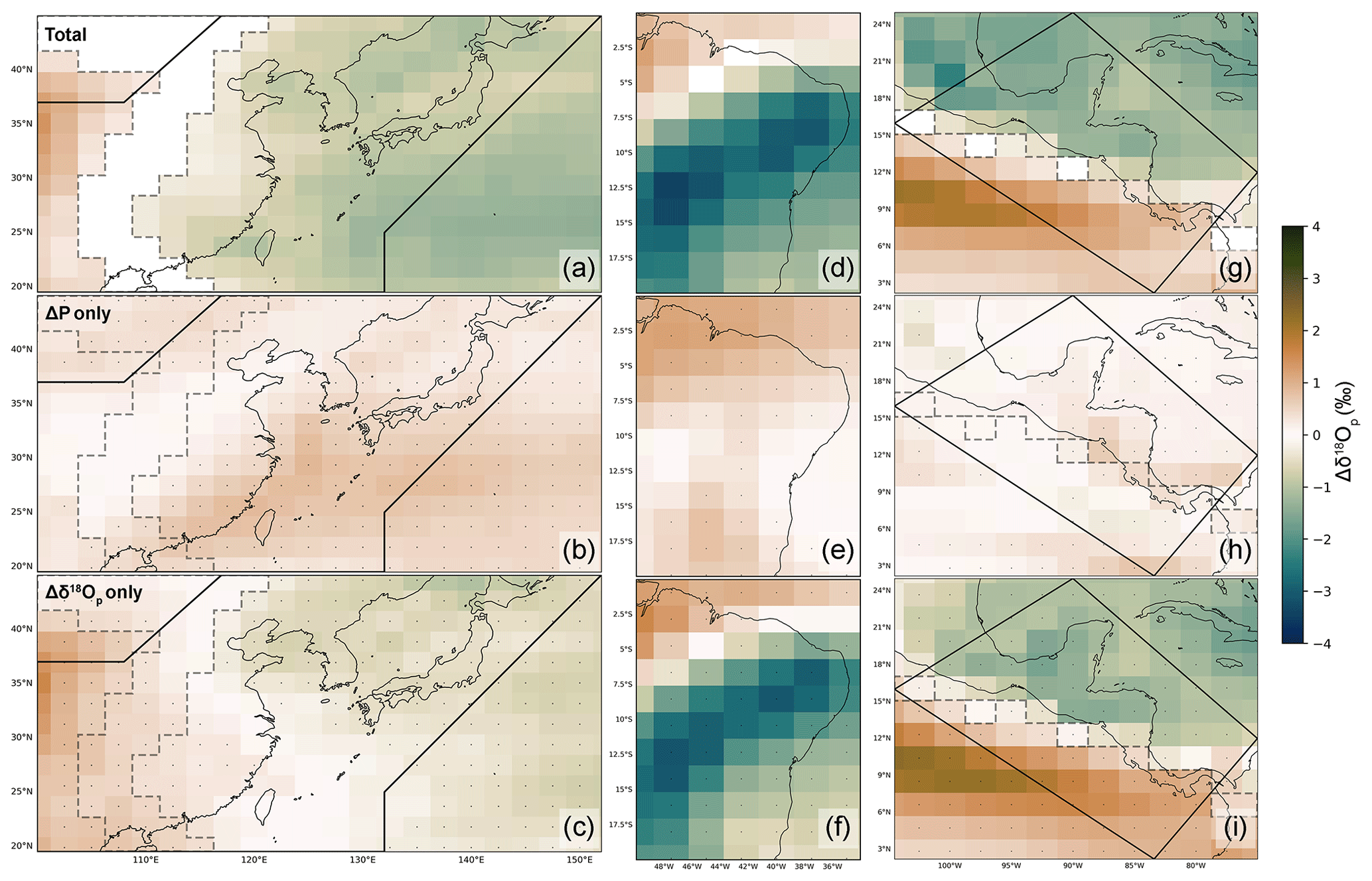
Figure 10 As in Fig. 9, but for East Asia (left column; a, b, c), northeast South America (middle column; d, e, f), and southern Central America (right column; g, h, i). The panels in the upper row show the annual amount-weighted δ¹⁸O_p anomaly in each region. The middle panels depict the contribution of the changes in the amount of monthly precipitation to the total change in amount-weighted δ¹⁸O_p, while the bottom panels depict the contribution of the monthly changes in δ¹⁸O_p. The unfilled black polygons represent the boundaries of each IPCC region. The grey dotted lines subdivide East Asia and southern Central America into E–W and N–S subregions defined by distinct ±Δδ¹⁸O_p dipoles shown in panels (a) and (g), respectively.

In northeastern South America and Central America, the change in amount-weighted δ¹⁸O_p is also dominated by changes in δ¹⁸O_p and not the seasonality of precipitation (Fig. 10d–f, g–i), although the mechanisms differ from those in East Asia. In northeastern Brazil, precipitation becomes more isotopically depleted as it intensifies during the wet season from December to July (Fig. 11c, d). These changes are consistent with a Type-1 control on δ¹⁸O_p (Lewis et al., 2010), wherein the local amount effect dominates the δ¹⁸O_p response. In Central America, the change in amount-weighted δ¹⁸O_p is characterized by a distinct SW–NE dipole with isotopic enrichment in the northeastern tropical Pacific and in southernmost Central America (Panama and Costa Rica), and isotopic depletion over the Caribbean and the remainder of Central America. This pattern is also driven by the seasonal changes in δ¹⁸O_p under meltwater forcing (Fig. 10h, i). In the northeastern tropical Pacific, Panama, and Costa Rica, wet season precipitation is substantially weakened and isotopically enriched (Fig. 13a, c), consistent with a Type-1 site (Lewis et al., 2010), wherein the local amount effect dominates the δ¹⁸O_p response. Past studies on the hydroclimate response to Heinrich events have shown that regional precipitation changes in northeastern Brazil and the eastern Pacific are associated with a southward shift of the Atlantic and northeastern tropical Pacific ITCZs (Lewis et al., 2010; Roberts et al., 2017; Atwood et al., 2020). However, the δ¹⁸O_p response over the Caribbean and the remainder of Central America is notably different. In this region, the wet season precipitation decreases under hosing, essentially eliminating the wet season, while the precipitation becomes substantially more isotopically depleted throughout the year (Fig. 13b, d), in association with the strong surface cooling and the addition of isotopically depleted meltwater to the North Atlantic. Thus, the δ¹⁸O_p response in this region would be classified as Type-5 according to the categorization of Lewis et al. (2010), with the mechanisms of the δ¹⁸O_p response governed by processes outside of the local or nonlocal amount effect, moisture source shifts, or seasonality of precipitation.

Table 3 Start, end, and duration of the 8.2 ka Event in the global compilation and the four regions discussed in this study.

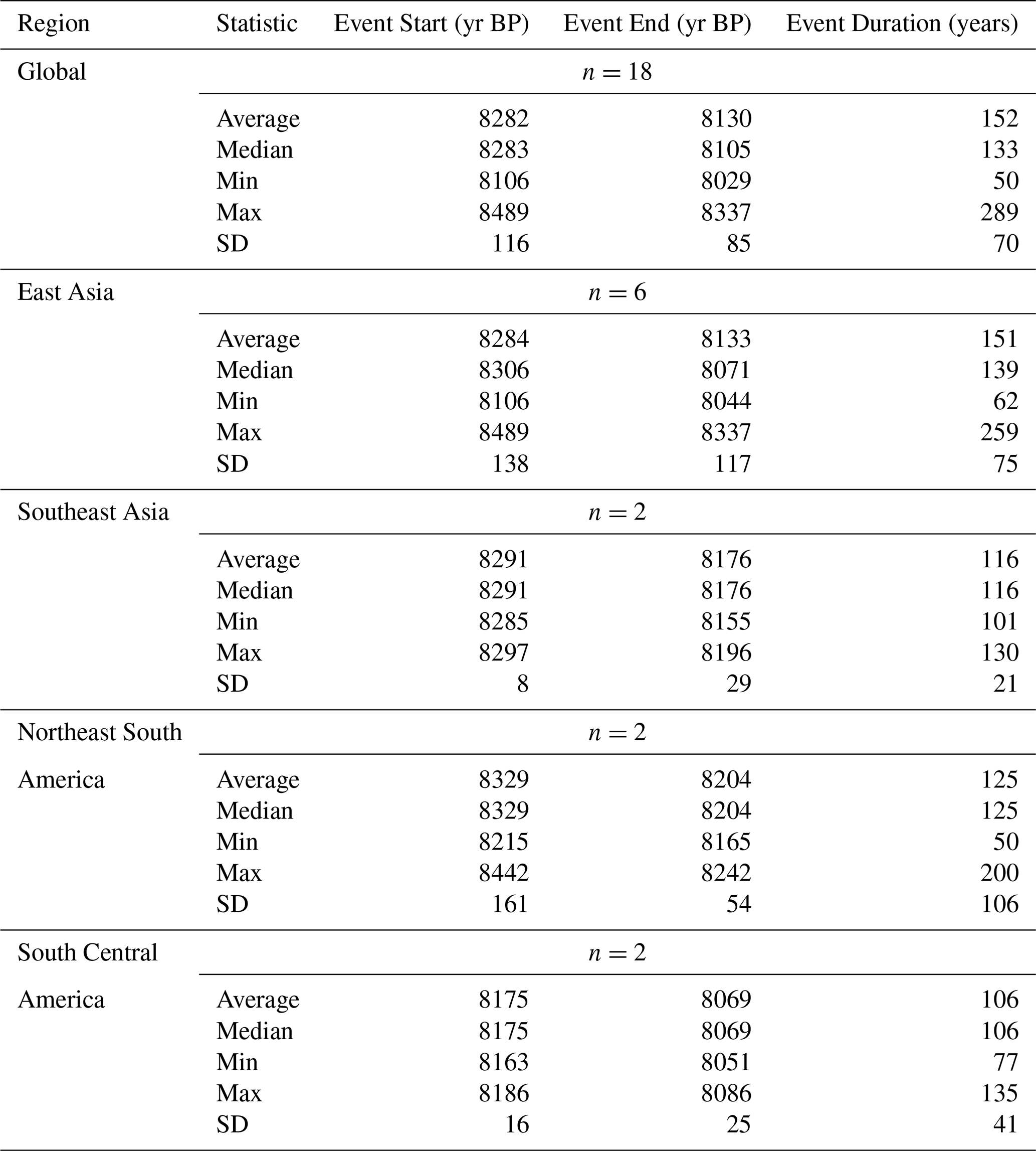
Table 4 Regional and global summary of 8.2 ka events detected by actR and our MM classification methods, separated by the sign of the anomaly (“wetter”, “drier”, and “no change”).

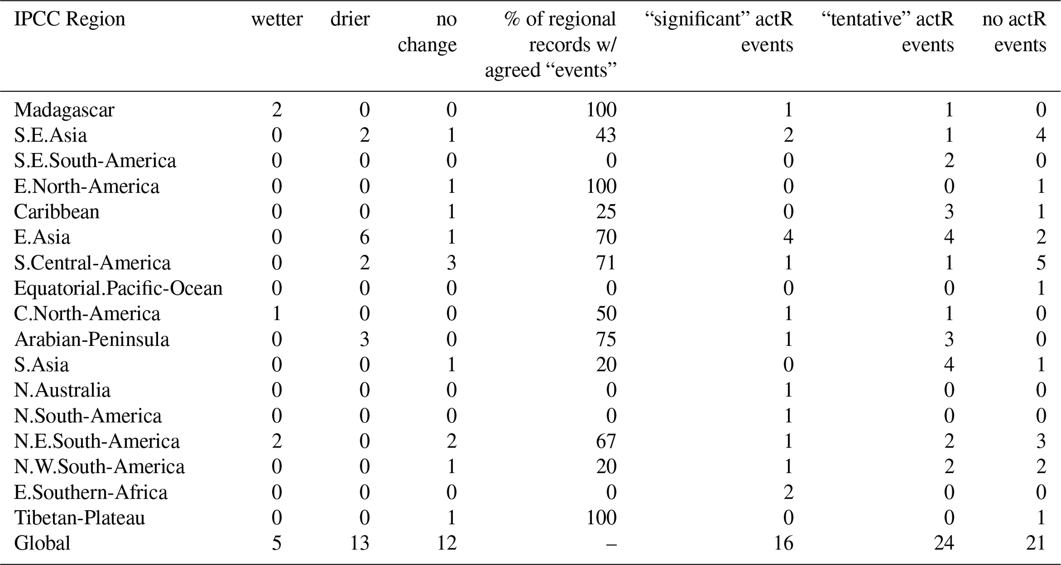
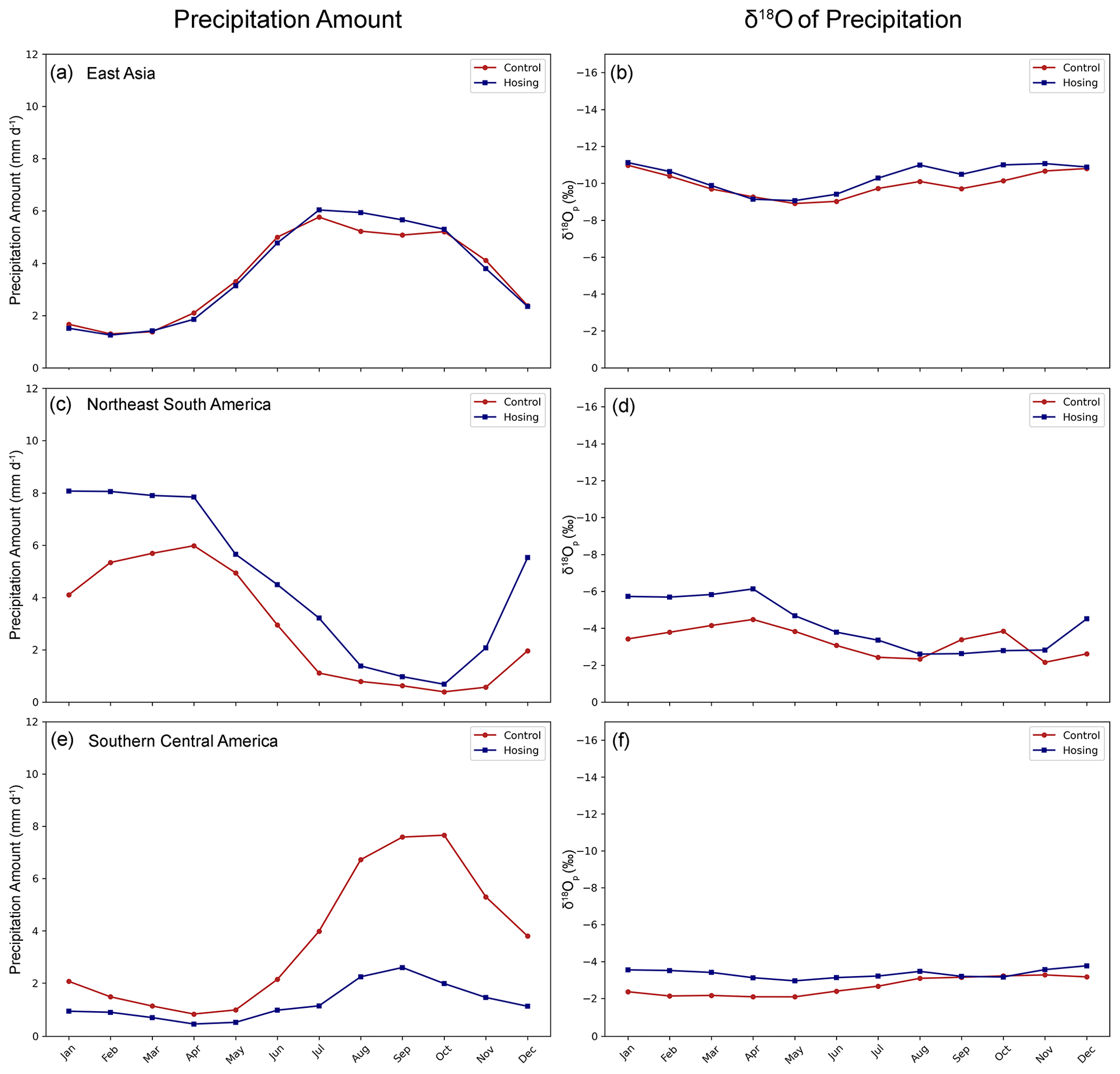
Figure 11 The area-weighted monthly average precipitation amount (left column) and δ¹⁸O of precipitation (right column) for the “ctrl” (red) and “hose” (blue) simulations for (a, b) East Asia, (c, d) northeast South America, and (e, f) southern Central America.

3.5 Data-model comparisons

The proxy locations span 17 IPCC scientific regions (Fig. B2). The regions with densest Tier 1 proxy data coverage are southern Central America, northeastern South America, East Asia, and Southeast Asia/Maritime Continent. These four regions were therefore targeted for data-model comparisons. The proxy records within each region were compared to model-simulated anomalies in annual mean precipitation amount, amount-weighted δ¹⁸O_p, and effective moisture (P-E) to investigate data-model agreement in the four target regions.

In East Asia (Fig. 5; Tables 3 and 4), five speleothem records display isotopic enrichment events broadly corresponding to the large-scale enrichment pattern in δ¹⁸O_p simulated by iCESM across South Asia and the Arabian Peninsula (Fig. 5a, b). This modeled enrichment pattern corresponds well with the broad isotopic enrichment found in proxy reconstructions spanning East Asia, the Arabian Peninsula, and southern Thailand. In iCESM, the Chinese speleothem records are located near the node of an east-west dipole pattern in δ¹⁸O_p in eastern China, which is part of a larger zonal pattern of δ¹⁸O_p anomalies, characterized by isotopic enrichment in the Middle East and Asia, and isotopic enrichment in the subtropics and extratropics of the North Pacific, extending into the eastern coast of China (Fig. 4a). This pattern was also noted in the 8.2 ka and Heinrich meltwater events performed with GISS ModelE-R (LeGrande and Schmidt, 2008; Lewis et al., 2010). Using vapor source distribution tracers, Lewis et al. (2010) identified changes in circulation, moisture source, and upwind processes as the dominant processes underpinning the δ¹⁸O_p response in the East Asian monsoon region in their Heinrich simulations. In agreement with their results, the enriched δ¹⁸O_p anomalies over Asia in the iCESM meltwater simulations do not appear to be driven by a weakened monsoon via a local amount effect, as the rainfall changes in the region are weak and spatially variable.

Table 5 The timing, duration, magnitude, and interpretation of the 8.2 ka Event for records with agreement between MM and actR methods. “N/A” signifies that we detected no event in the associated record using either method.

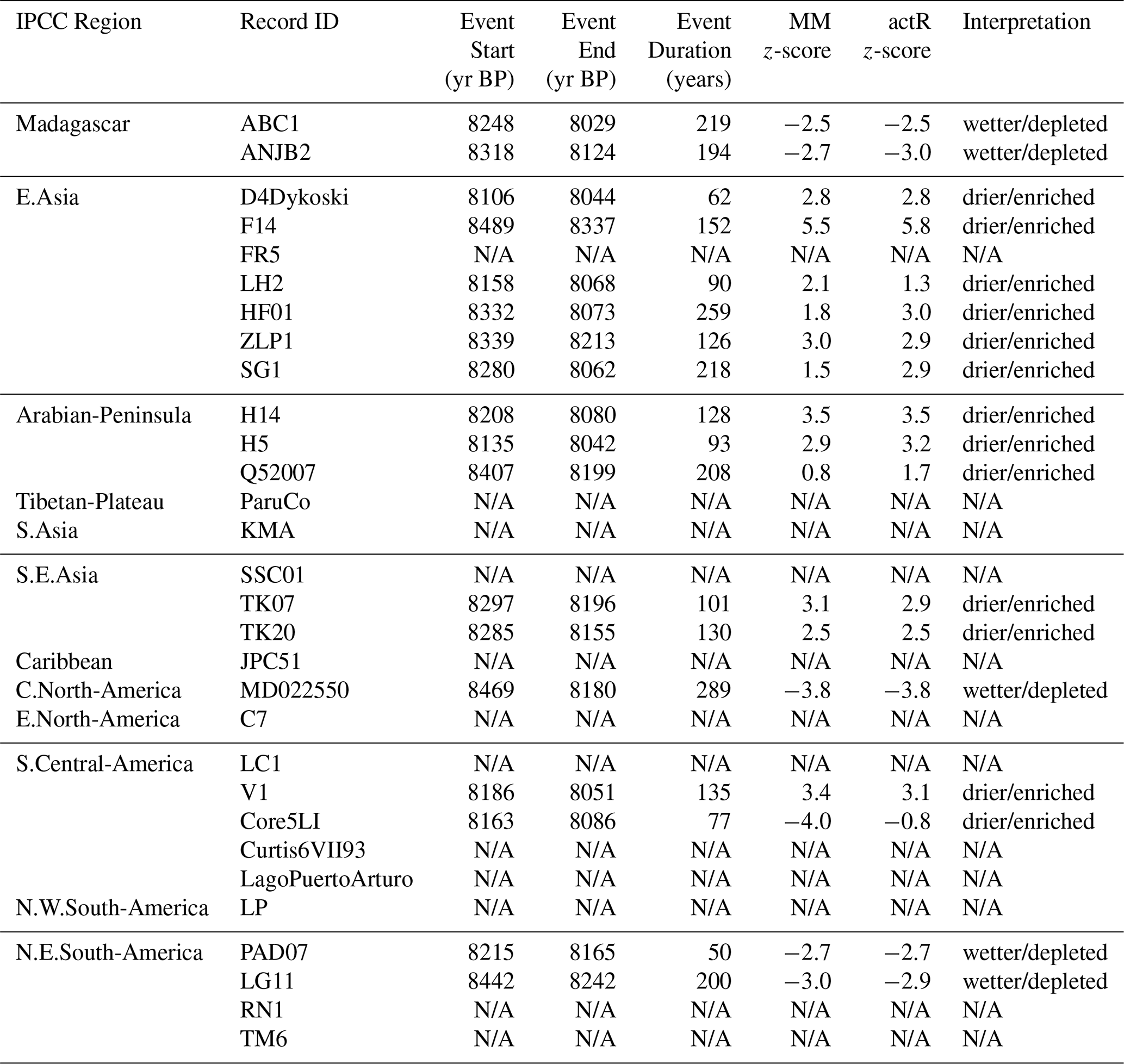
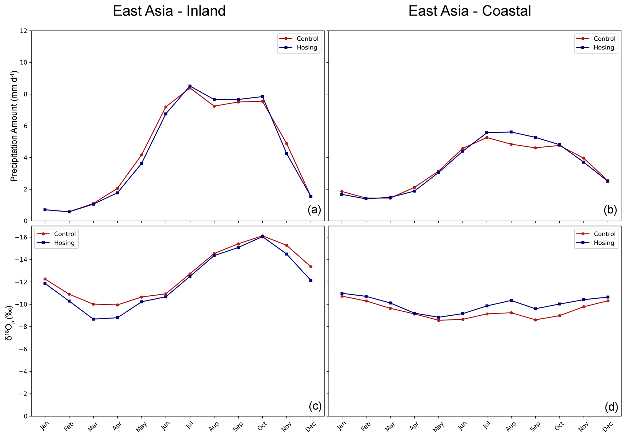
Figure 12 The monthly climatology of the area-weighted precipitation amount (a, b) and δ¹⁸O_p (c, d) in East Asia for the “ctrl” (red) and “hose” (blue) simulations. Data from the western (inland) subregion defined by the positive Δδ¹⁸O_p anomaly in Fig. 10a are plotted in the left column. Data from the eastern (coastal) subregion defined by the negative Δδ¹⁸O_p anomaly are plotted in the right column.

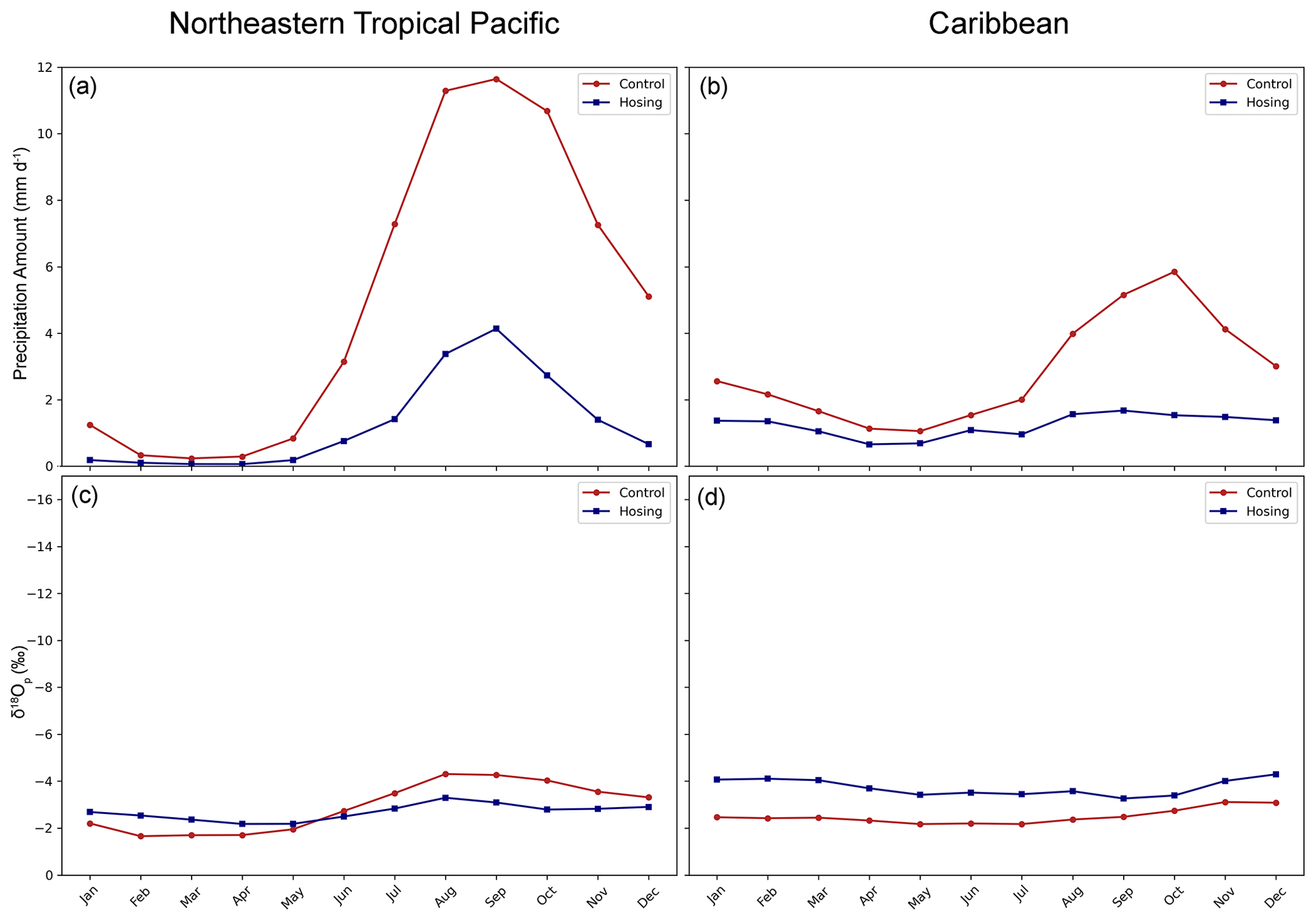
Figure 13 As in Fig. 12, but for Southern Central America. Data from the southern subregion (northeastern tropical Pacific) defined by the positive Δδ¹⁸O_p anomaly in Fig. 10g are plotted in (a) and (c), while data from the northern subregion (Caribbean) defined by the negative Δδ¹⁸O_p anomaly in Fig. 10g are plotted in (b) and (d).

Northeastern South America displays only moderate proxy-model agreement (Fig. 6). Two of the four speleothem records there contain large δ¹⁸O depletion events, corresponding with the large-scale isotopic depletion signal in δ¹⁸O_p in iCESM across northeastern South America. However, two other speleothem records in the region – one in the Nordeste region of Brazil and one in central Brazil – show no significant hydroclimate anomalies during the 8.2 ka Event, in contrast with the results from iCESM.

In Central America, the simulated and reconstructed hydroclimate anomalies broadly agree (Fig. 7), with the dry event in the Guatemalan lake sediment record of Core5LI (Duarte et al., 2021) corresponding with the reduced precipitation throughout Central America simulated in iCESM. The lack of a detected event in three lake sediment records from the Yucatan Peninsula (LagoPuertoArturo, Curtis6VII93, LC1) also agrees with the simulated weak EM response in that region in iCESM. A positive δ¹⁸O_p event in the Costa Rican speleothem record (V1; Lachniet et al., 2004) agrees in sign with enriched δ¹⁸O_p in southernmost central America in iCESM, though the cave site sits at the nodal point of a pronounced east-west dipole pattern in δ¹⁸O_p in iCESM, with widespread isotopic enrichment in δ¹⁸O_p in the eastern tropical Pacific and widespread isotopic depletion in the tropical North Atlantic that stretches into the Caribbean and all but the southernmost part of Central America. Using this regional context, the isotopic enrichment event in Costa Rica is consistent with the simulated enrichment in δ¹⁸O_p that extends from southernmost Central America to the eastern tropical Pacific.

Broad data-model agreement is also found in Southeast Asia and the Maritime Continent (Fig. 8), where one speleothem record in the Thailand peninsula contains a notable isotopic enrichment event, in agreement with the simulated large scale enrichment signal in δ¹⁸O_p in South Asia (Figs. 8 and B8). Two other speleothem records in Sumatra and Borneo show no significant hydroclimate anomalies, in general agreement with the weak simulated δ¹⁸O_p anomalies in iCESM in this region, which reflect the weak response in δ¹⁸O_p throughout the western Pacific and Maritime Continent (Fig. 4a).

These results suggest that iCESM captures many of the regional hydroclimate responses observed in the reconstructions, including the large-scale isotopic enrichment pattern in δ¹⁸O_p in South and East Asia and the Arabian Peninsula, the muted hydroclimate response in the Maritime Continent, the mixed hydroclimate patterns in Central America, and the isotopic depletion in δ¹⁸O_p in parts of eastern Brazil. Similar hydroclimate features also appear in simulations of the Younger Dryas cold event from Renssen et al. (2018). While qualitative, these areas of agreement between the proxies and model demonstrate that the tropical hydroclimate response to North Atlantic meltwater forcing during the 8.2 ka Event was not a simple hemispheric dipole pattern, but is instead characterized by rich regional structure.

While qualitative agreement exists between many of the reconstructed and simulated regional hydroclimate anomalies during the 8.2 ka Event, our data-model comparisons are subject to several limitations. First, our regional analyses are limited by small sample sizes. In some regions like East Asia, point-to-point agreement between proxy and model data is low even though regional hydroclimate patterns offer more nuanced context. In addition, our data-model comparisons are necessarily qualitative as many of the proxy records in our compilation are carbonate δ¹⁸O records, which do not solely reflect changes in δ¹⁸O_p. Rather, these archives incorporate a combination of the isotopic composition of groundwater (for speleothem δ¹⁸O records; Lachniet, 2009) or seawater (for marine δ¹⁸O records; Konecky et al., 2020) as well as the environmental temperature, among other factors (LeGrande and Schmidt, 2009; Bowen et al., 2019; Konecky et al., 2019). Thus, future work should integrate proxy system models with water isotope-enabled climate model simulations to develop more quantitative data-model comparisons of the 8.2 ka Event. In addition, quantitative metrics like the weighted Cohen's kappa statistic could be used to quantitatively compare the proxy reconstructions to the pseudoproxy data derived from climate models (Cohen, 1960, 1968; Landis and Koch, 1977; DiNezio and Tierney, 2013).

However, even when attempting to bridge the gap between models and proxy data using proxy system models and quantitative metrics, robust comparisons remain challenging. Characterizing the point-to-point agreement between the observed and simulated climate anomalies fails to address the well-known hydroclimate biases that exist in GCMs, which arise from factors like course model resolution, idealized topography, and the unresolved physics of cloud formation and convection. Furthermore, proxy data often capture localized climate signals which may not be representative of regional conditions. In contrast, model data are averaged over the area of a grid cell, which can be large in coarse-resolution models. This can lead to non-trivial biases, particularly in coastal regions and regions of complex topography. Ultimately, these data-model comparisons would be improved by the integration of additional well-dated proxy records that resolve different aspects of hydroclimate, and employing ensembles of high-resolution water isotope-enabled climate model simulations of the 8.2 ka Event paired with proxy system models.

4 Discussion

4.1 Comparison to previous hydroclimate compilations

The spatial pattern of hydroclimate responses to the 8.2 ka Event presented in this study broadly agrees with Morrill et al. (2013) and Parker and Harrison (2022). All three studies document large-scale drying across East Asia and the Arabian Peninsula, alongside robust wet and/or isotopic depletion signals in central and eastern Brazil. These signals coincide with drying and/or isotopic enrichment events in northern South America, aligning with the simulated hydroclimate response in iCESM (Fig. 4). All three reconstructions also broadly agree on the hydroclimate signals across Central America, with Morrill et al. (2013) inferring dry conditions from lake records, and Parker and Harrison (2022) identifying a mixed signal in speleothem records with positive isotopic anomalies in the southerly sites and negative anomalies in the more northern sites, the latter of which they speculate reflects the lower δ¹⁸O of seawater in the Gulf of Mexico observed in a marine δ¹⁸O record. These features agree well with the present study, in which the Central American proxies are well captured by the hydroclimate response in iCESM, which features a southward shift of the Pacific and Atlantic ITCZs that drive pronounced drying across Central America and an associated enriched δ¹⁸O_p response in southernmost Central America, and isotopic depletion throughout the rest of Central America likely associated with the upwind cooling of SSTs and addition of isotopically depleted meltwater in the North Atlantic.

Timing and duration estimates also show reasonable agreement across compilations. Our age ensembles yield a mean start age of 8.28 ± 0.12 ka (1σ), a termination age of 8.11 ± 0.09 ka (1σ), and an average duration of 152 ± 70 years (1σ; 50–289 years). These results agree, within age uncertainty, to the initiation and termination of the global event estimated from northern Greenland ice core data (8.09–8.25 ka; Thomas et al., 2007). Previous studies report comparable findings. Using eight absolutely dated speleothems from China, Oman, and Brazil, Cheng et al. (2009) estimated the onset of the 8.2 ka Event at 8.21 ka, termination at 8.08 ka, and a total duration of 130–150 years. Parker and Harrison (2022) refined these estimates using 275 absolutely dated speleothems, calculating the global onset at 8.22 ± 0.01 ka, termination at 8.06 ± 0.01 ka, and a duration of 159–166 years. While our range of event durations exceeds those in Cheng et al. (2009) and Parker and Harrison (2022), it is consistent with the estimated range of 40–270 years from the multiproxy compilation of Morrill et al. (2013). Importantly, the present study is the first to comprehensively account for age uncertainty by propagating age ensembles through all phases of event detection. Our larger uncertainties and duration range likely stem from this explicit treatment of age uncertainty, combined with the inclusion of lower-resolution lake and marine sediment records alongside higher-resolution speleothems in our compilation. In all cases, the average event duration in the hydroclimate records closely resembles that in the layer-counted Greenland ice core records (160.5 ± 5.5 years; Thomas et al., 2007), providing further support of the global and synchronous nature of the 8.2 ka Event.

One striking difference between our compilation and previous studies is the relatively low percentage of records with detected 8.2 ka Events (e.g., only 30 % of our records, compared to 70 % in Parker and Harrison's, 2022 global speleothem compilation). This difference may arise from several factors. We focus exclusively on tropical proxy data, which are likely to record weaker anomalies than proxies from the North Atlantic and Europe, regions more directly impacted by proximity to the meltwater forcing. More importantly, our explicit accounting of age uncertainty reveals that many records lack sufficient age constraints, precluding the generation of age ensembles to pass the robust null hypothesis test in actR, and thereby fail to identify abrupt anomalies attributable to the 8.2 ka Event.

4.2 Comparison of the simulated 8.2 ka Event across models

Two lower-resolution isotope-enabled GCM simulations have previously been conducted to investigate the 8.2 ka Event. LeGrande and Schmidt (2008) used the Goddard Institute for Space Studies ModelE-R (GISS ModelE-R) to evaluate the response of global temperatures, precipitation amount, and δ¹⁸O_p values to a slowdown of the AMOC. GISS ModelIE-R is a fully coupled GCM from the IPCC AR4 era, featuring a 4°×5° horizontal resolution atmosphere model coupled with an ocean model of the same resolution, comprising 20 and 13 vertical layers, respectively. LeGrande and Schmidt (2008) performed a 1000-year preindustrial control simulation and a suite of twelve meltwater forced experiments, applying a range of forcings (1.25 to 10 Sv) over the Hudson Bay for 0.25 to 2 years. They found that this range of meltwater forcings inhibited North Atlantic Deep Water (NADW) formation and reduced the strength of the AMOC for up to 180 years.

In agreement with the results from iCESM, LeGrande and Schmidt (2008) found large δ¹⁸O_p anomalies over the meltwater source area in the North Atlantic in the decade following the meltwater forcing, which they similarly attributed to the evaporation and rainout of the isotopically depleted meltwater in the region. They observed reasonable agreement between their simulations and proxy records of temperature and hydroclimate, with the simulations containing larger meltwater forcing exhibiting better agreement with the proxies (emphasizing the importance of considering an ensemble of simulations to find the best fit to proxy reconstructions). Regarding the tropical hydroclimate response, they identified bands of enriched (depleted) δ¹⁸O_p anomalies in the northern (southern) tropics as a result of a southward shift in tropical rainfall. Notable patterns of δ¹⁸O enrichment were identified in northeastern Africa, through the Middle East, South Asia, and the Thailand peninsula, which they attributed to large-scale changes in the hydrologic cycle, including shifts in moisture source and moisture transport pathways.

In a more recent set of simulations, Aguiar et al. (2021) used the University of Victoria Earth System Climate Model version 2.9 (UVic ESCM2.9) with the addition of oxygen isotopes to test proxy-model agreement under a range of empirically derived freshwater forcing scenarios. UVic ESCM2.9 uses the Modular Ocean Model version 2, with a horizontal resolution of 3.6° longitude ×1.8° latitude and 19 vertical levels. The version of the UVic ESCM2.9 model used in this study possesses a simple two-dimensional atmospheric energy moisture balance model, which limits its ability to accurately represent δ¹⁸O_p values. Aguiar et al. (2021) compared the sea surface temperatures and seawater δ¹⁸O values from 28 simulations with 35 proxy records to place new constraints on the amount and rate of freshwater forcing in the North Atlantic. Their analysis revealed that a two-stage meltwater experiment with a background flux of 0.066 Sv over 1000 years (8–9 ka), followed by an intensification to 0.19 Sv over 130 years (8.18–8.31 ka), best replicated the anomalies observed in the proxy records.

The iCESM simulation illustrates clear signatures of the meltwater forcing that, at the largest scales, are broadly consistent with the GISS and UVic simulations described above, including the hemispheric dipole pattern in temperature and associated southward shift of the tropical rainbands. On regional scales, the tropical rainfall patterns display substantial regional heterogeneity, with a southward shift of the tropical ocean rain bands, drying in the major NH monsoon regions of South Asia and West Africa, and wetting in parts of the South American Summer Monsoon. Tropical δ¹⁸O_p values display strong signatures of the 8.2 ka Event, including opposing patterns of δ¹⁸O_p values between northern South America and northeastern Brazil (e.g., Zhu et al., 2017) and large δ¹⁸O_p anomalies over the meltwater region (e.g., LeGrande and Schmidt, 2008; Bowen et al., 2019). Dry (wet) anomalies correspond with enriched (depleted) δ¹⁸O_p values in some tropical regions, implicating the “amount effect” as the driving force behind the isotopic signal, but a decoupling of precipitation amount and δ¹⁸O_p anomalies occurs over many tropical continental regions, indicating that other processes such as changes in moisture source, moisture transport pathways, water recycling over land, and/or changes in precipitation seasonality, dominate the isotopic signal in those regions. The model simulations lend support to the proxy reconstructions in demonstrating that the tropical hydroclimate response to the 8.2 ka Event cannot be described as a simple hemispheric dipole pattern, particularly over continental regions, and that the rich regional structure of the precipitation amount and δ¹⁸O_p responses must be considered in order to understand the full picture of the tropical hydroclimate response to this event.

5 Conclusions

This study has investigated the tropical hydroclimate response to the 8.2 ka Event in a new multi-proxy data compilation and isotope-enabled model simulation. Two event detection methods were used in this study. The first method relies on the original age model of each record while the second method implements a changepoint detection algorithm that explicitly accounts for age uncertainties in each proxy record. In order to leverage the strengths of each method and provide a more robust reconstruction of the hydroclimate response to the 8.2 ka Event, only records in which events were detected in both event detection methods were used to characterize the hydroclimate response to the 8.2 ka Event.

Robust hydroclimate anomalies were detected in 18 records across the 7.9–8.5 ka interval while 12 records showed no evidence of a hydroclimate anomaly associated with the 8.2 ka Event. Across the records with a detected hydroclimate event, a mean onset age of 8.28 ± 0.12 ka (1σ), mean termination age of 8.11 ± 0.09 ka (1σ), and mean duration of 152 ± 70 years (1σ; with a range of 50 to 289 years) was found, comparing well with previous estimates. Importantly, this work is the first to explicitly account for age uncertainty through all phases of the event detection analysis.

The results demonstrate that the tropical hydroclimate response to the North Atlantic meltwater forcing was not a simple hemispherically uniform dipole pattern but is better characterized by rich regional structure. Coherent regional hydroclimate changes identified in the proxy records include pronounced isotopic enrichment across East Asia, South Asia, and the Arabian Peninsula. In the Americas, drying and isotopic enrichment occurred in Central America south of the Yucatán Peninsula, contrasting with isotopic depletion in eastern Brazil. In contrast, no signatures of the 8.2 ka Event were found over the Maritime Continent.

The isotope-enabled model simulation with iCESM illustrates clear signatures of the global 8.2 ka Event that are largely consistent with the proxy records. Large-scale cooling in the Northern Hemisphere and warming in the Southern Hemisphere drives a southward shift of tropical rainfall but with highly variable regional patterns. Major features include a southward shift of the tropical ocean rain bands in the tropical Atlantic, Central and Eastern Pacific, and Indian Oceans (characterized by a weakening of the northern extent and enhancement of the southern extent of the rainbands), as well as drying in Central America and northern South America and wetter conditions in northeastern Brazil. Modest drying also occurs in the Northern Hemisphere monsoon regions of South Asia and West Africa. The simulated isotopic composition of tropical precipitation also displays strong signatures of the meltwater event. Over land, δ¹⁸O_p displays a pronounced dipole pattern in South America, with isotopic enrichment in northern South America and isotopic depletion in northeastern Brazil. Large-scale isotopic depletion also occurs over the Arabian Peninsula and South Asia. Over the tropical oceans (excluding the western tropical Pacific), a pronounced north-south dipole pattern occurs in δ¹⁸O_p, with isotopic enrichment corresponding with drier conditions north of the equator and isotopic depletion corresponding with wetter conditions south of the equator. Precipitation amount and δ¹⁸O_p anomalies are more muted in the Western Pacific, Maritime Continent, and Africa. We decompose the simulated δ¹⁸O_p response to identify the causes of these isotopic anomalies in the tropics, finding that changes in amount-weighted δ¹⁸O_p arise primarily from changes in the isotopic composition of precipitation rather than changes in precipitation seasonality. However, the mechanisms of the changes in δ¹⁸O_p vary regionally, with the local amount effect dominant in northeastern South America and the northeastern tropical Pacific; while changes in the isotopic composition of the water vapor (via changes in moisture source, circulation, and/or upstream rainout) seem to control the response in East Asia; cooler SSTs and the addition of isotopically depleted meltwater to the North Atlantic directly contributes to reduced, but isotopically depleted, wet season precipitation throughout the Caribbean, extending into all but the southernmost extent of Central America.

The proxy records were compared to simulated δ¹⁸O_p, precipitation amount, and effective moisture (P-E) from co-located sites in four regions with the densest coverage of proxy data: southern Central America, northeastern South America, East Asia, and Southeast Asia. Subject to the small sample sizes found in the regional data-model comparisons, the results suggest that iCESM captures many of the regional hydroclimate responses observed in the reconstructions, including the large-scale isotopic enrichment pattern in δ¹⁸O_p in South and East Asia and the Arabian Peninsula, mixed hydroclimate patterns in southern Central America, the isotopic depletion in parts of eastern Brazil, and the muted hydroclimate response in the Maritime Continent.

These results serve as a first step toward more quantitative data-model comparison studies. Recommendations for future studies include performing an ensemble of targeted 8.2 ka simulations with iCESM and other isotope-enabled climate models (with meltwater applied to the Labrador Sea), adding more well-dated proxy records that resolve different aspects of hydroclimate during the 8.2 ka Event, and quantitatively comparing these records with the simulations paired with proxy system models. Future work should also investigate the physical mechanisms of the simulated hydroclimate responses and their isotopic signatures to improve our understanding of the tropical hydroclimate response to abrupt climate change events.

Appendix A

Table A1 Age model information. In column three, “N/A” signifies that there is no published ¹⁴C calibration curve associated with a record because the record was dated using uranium series methods (i.e., $\mathrm{U}/\mathrm{Th}$ dating). In column six, “N/A” represents marine or lacustrine archives, which therefore do not appear in the SISALv2 database.

Appendix B

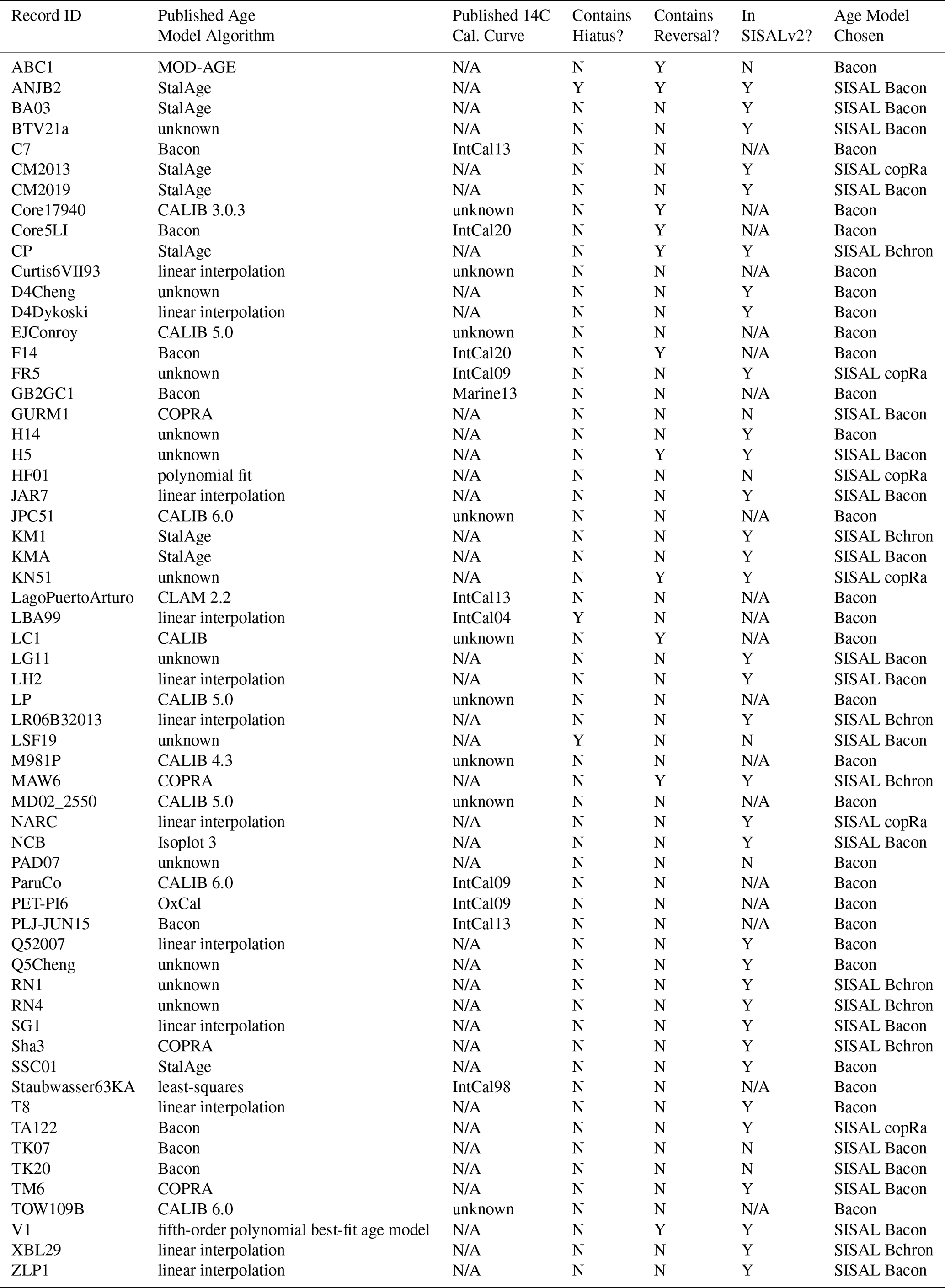
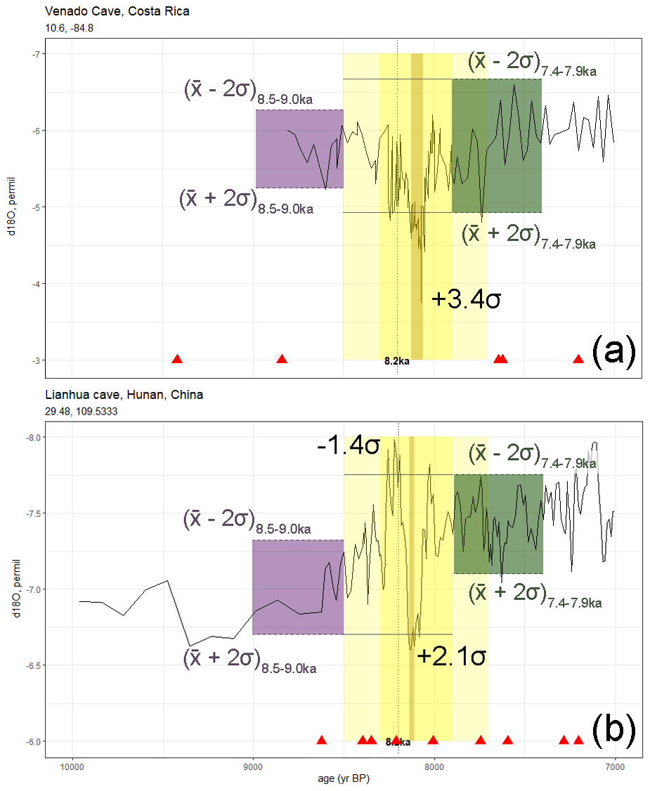
Figure B1 A schematic illustrating the application of our modified Morrill method to (a) the speleothem record of Lachniet et al. (2004) (V1) and (b) the record of Zhang et al. (2013) (LH2). The red triangles indicate the ages of radiometric dates associated with the proxy data. The green and purple shading represents $\stackrel{\mathrm{‾}}{x}$ ± 2σ in each reference window (7.4–7.9 and 8.5–9.0 ka, respectively). The top panel highlights an anomalous isotopic enrichment (“drier”; brown) event which is composed of three separate “events” (separated by <20 years). As per the event detection methods, these events have been consolidated into a single 8.2 ka Event (8.058–8.124 ka) with the event magnitude given by the maximum absolute z-score over this period (+3.4σ). The bottom panel shows multiple events of opposing signs within the detection window: an anomalous isotopic depletion (−1.4σ, 8.208–8.221 ka) and an anomalous enrichment (+2.1σ, 8.129–8.138 ka; brown). As per the event detection methods, the event with the larger absolute z-score is taken to represent the 8.2 ka Event.

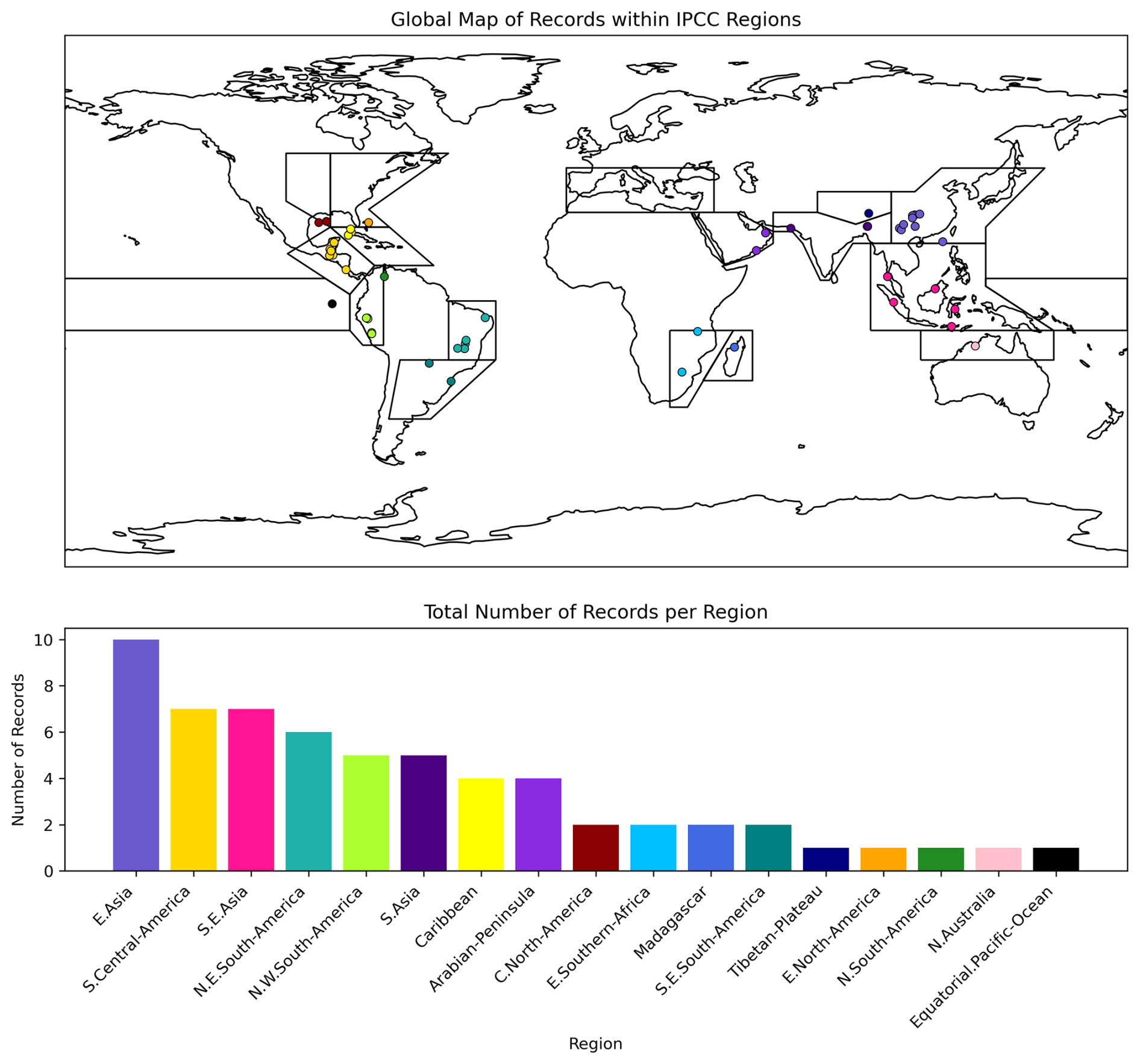
Figure B2 Locations of proxy records within climate reference regions defined in Iturbide et al. (2020).

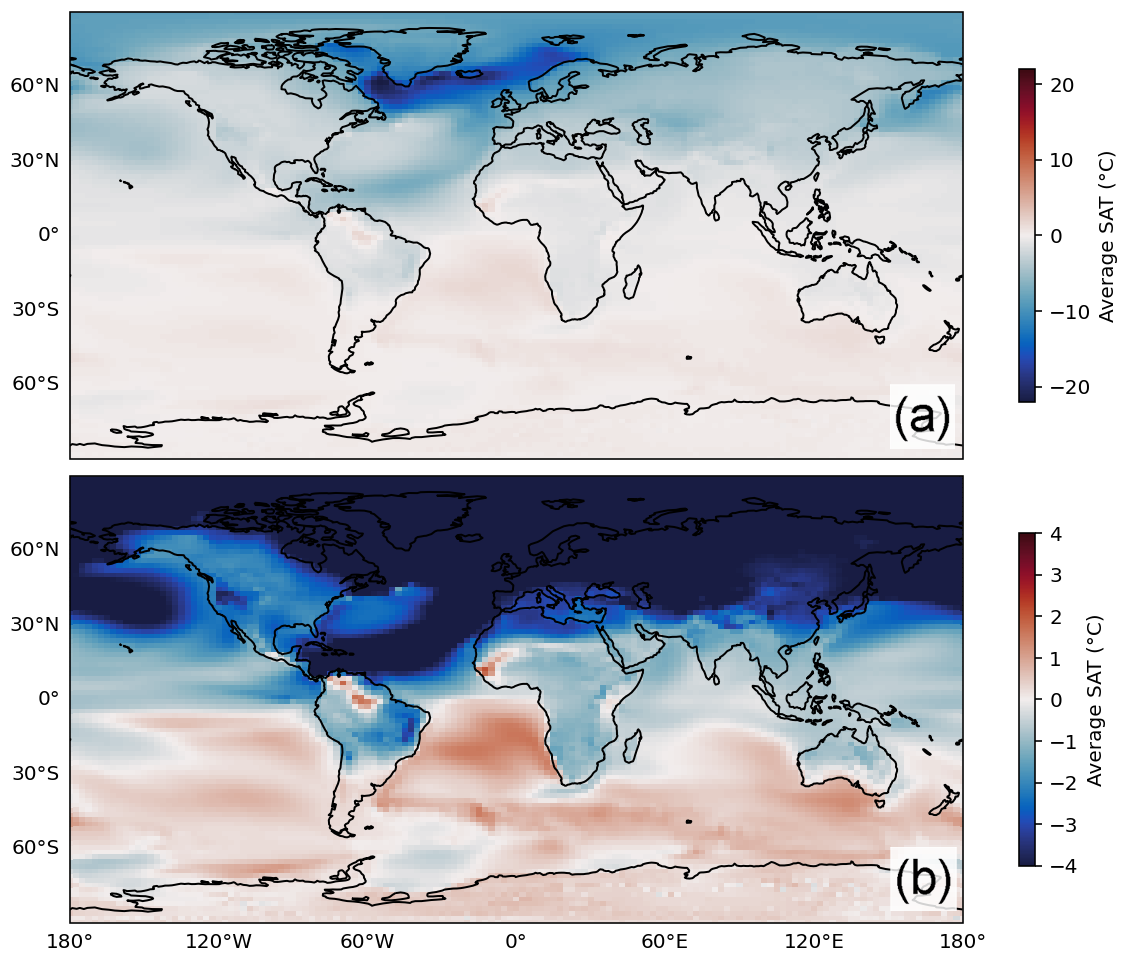
Figure B3 The difference in surface air temperatures between the last 50 years of the “hose” and “ctrl” simulations. Blue shaded areas represent anomalously cold regions, while anomalously warm regions are shaded in red on a global (a) and (b) tropical level.

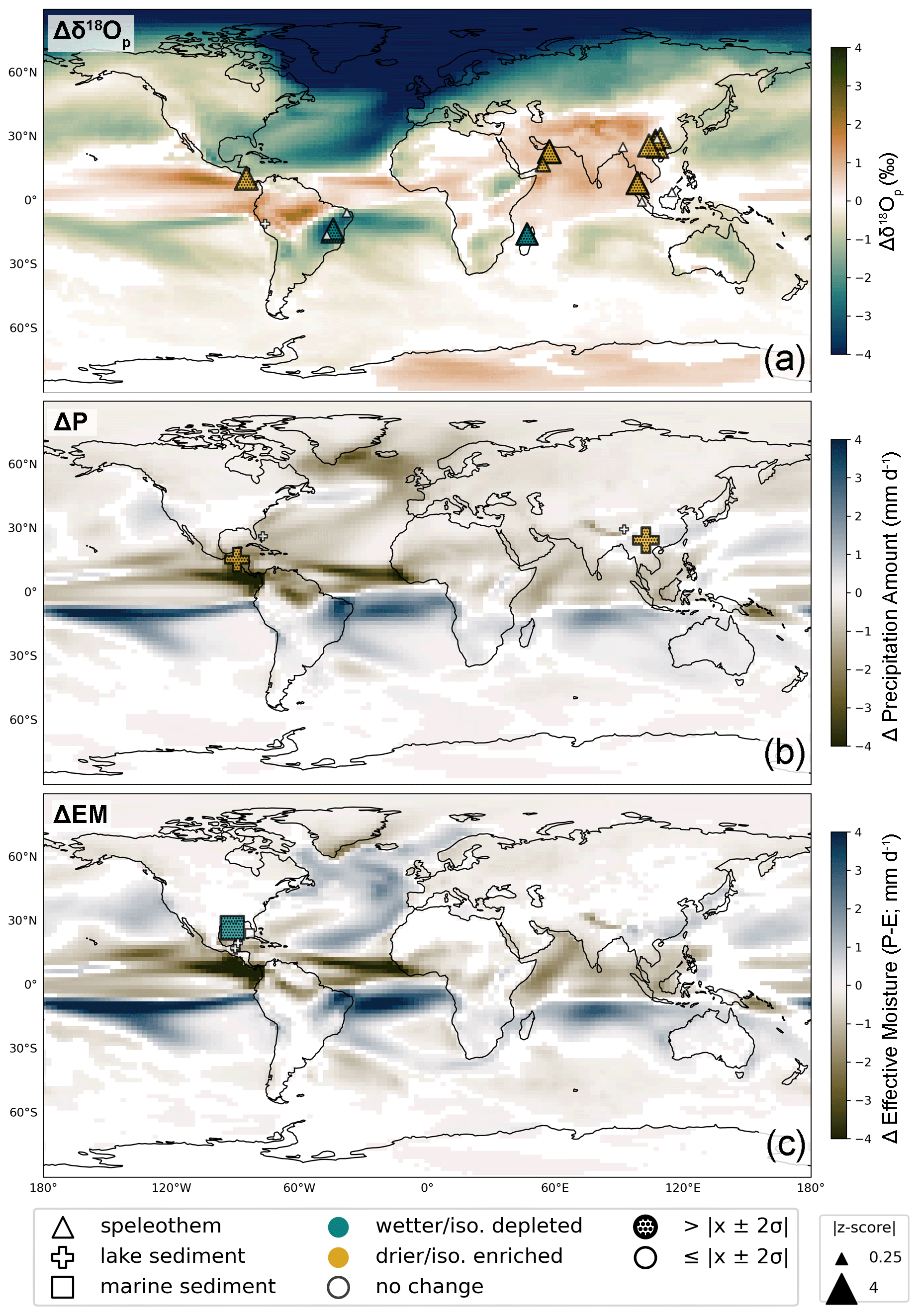
Figure B4 Summary of the 8.2 ka events detected using our modified Morrill et al. (2013) method for the paleoclimate records showing agreement with actR (Fig. 4) in the direction of change. Blue symbols represent wetter (and/or isotopically depleted) conditions while brown symbols represent drier (and/or isotopically enriched) conditions relative to each record's mean climatology over the 7.4–7.9 and 8.5–9.0 ka windows described in the text. For records in which no event was detected, symbols are shown in white. The archive type is indicated by the symbol shape, and the symbol size is scaled by $\mathrm{250}\ln (\mathrm{1}+|z\text{-score}\left|\right)$. The proxy symbols are overlaid on a contour map of the simulated anomalous (a) amount-weighted δ¹⁸O_p, (b) precipitation amount, and (c) effective moisture (P-E), calculated from the difference between the last 50 years of the iCESM “hose” and “ctrl” experiments, where only anomalies that exceed the 95 % confidence level (p<0.05) are shown.

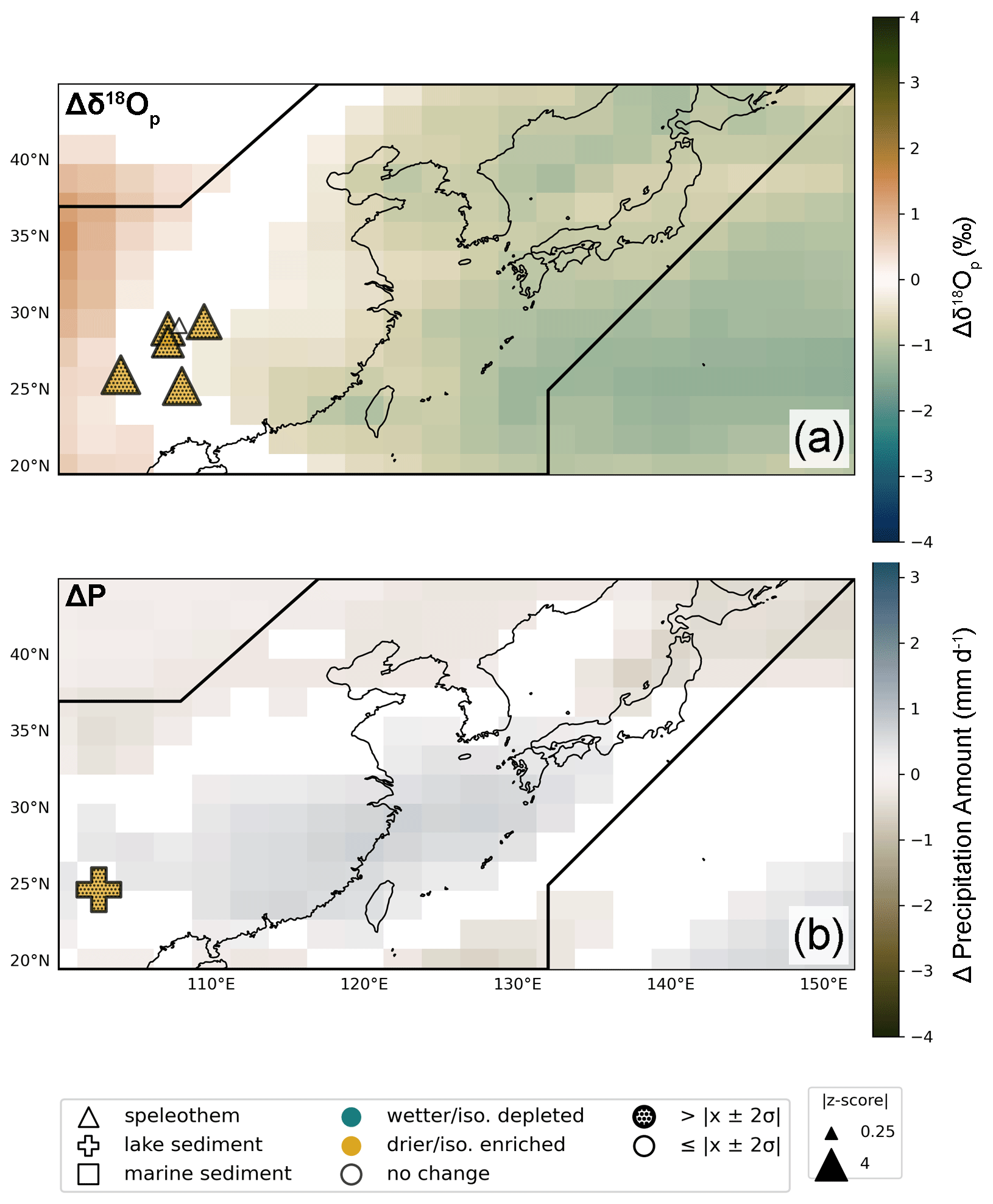
Figure B5 Data-model comparison of IPCC region 35: East Asia (box). Model shading represents (a) the amount-weighted δ¹⁸O_p anomaly, and (b) the precipitation amount anomaly between the last 50 years of the “hose” and “ctrl” simulations that exceed the 95 % confidence level (p<0.05). Symbols represent paleoclimate proxy archives within the region corresponding to each respective climate variable, where the brown shaded triangles indicate speleothem records with recorded dry hydroclimate/enriched isotopic anomalies during the 8.2 ka Event and grey symbols indicate records with no hydroclimate anomalies (”no change”) relative to each record's mean climatology over the 7.4–7.9 and 8.5–9.0 ka windows used in our modified Morrill et al. (2013) method. For symbols showing an anomaly associated with the 8.2 ka Event, size is scaled by $\mathrm{400}\ln (\mathrm{1}+|z\text{-score}\left|\right)$ relative to each record's mean and standard deviation.

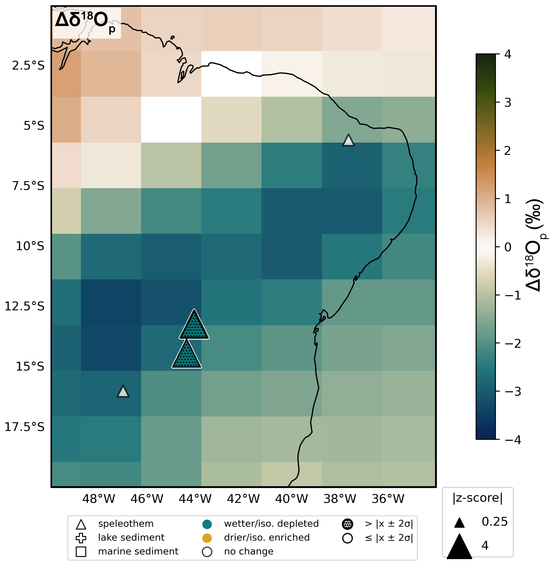
Figure B6 As in Fig. B5, but for IPCC region 11: northeastern South America (box).

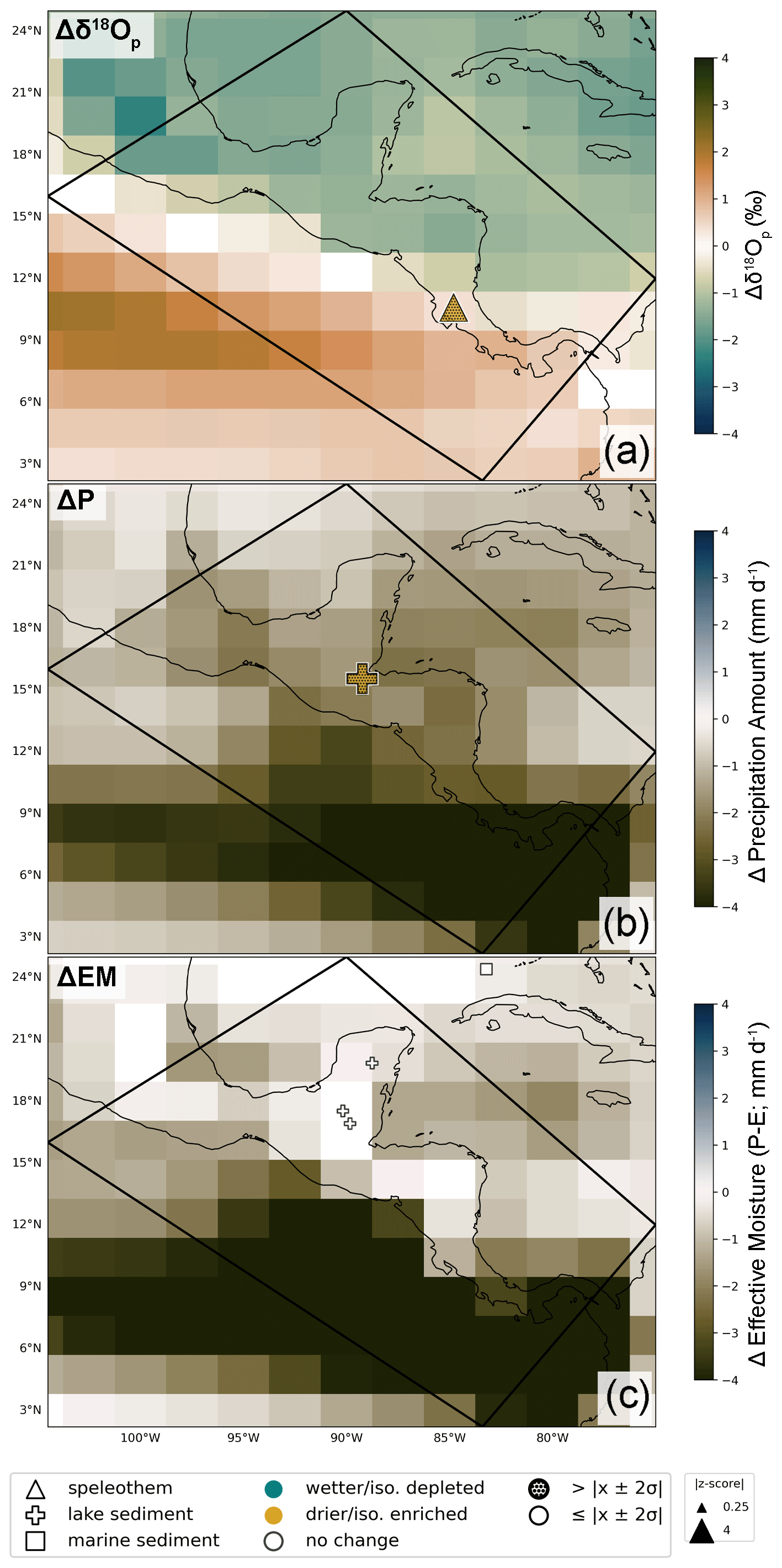
Figure B7 As in Fig. B5, but for IPCC region 7: southern Central America (box), with the addition of (c) the effective moisture (precipitation minus evaporation) anomaly between the last 50 years of the “hose” and “ctrl” simulations.

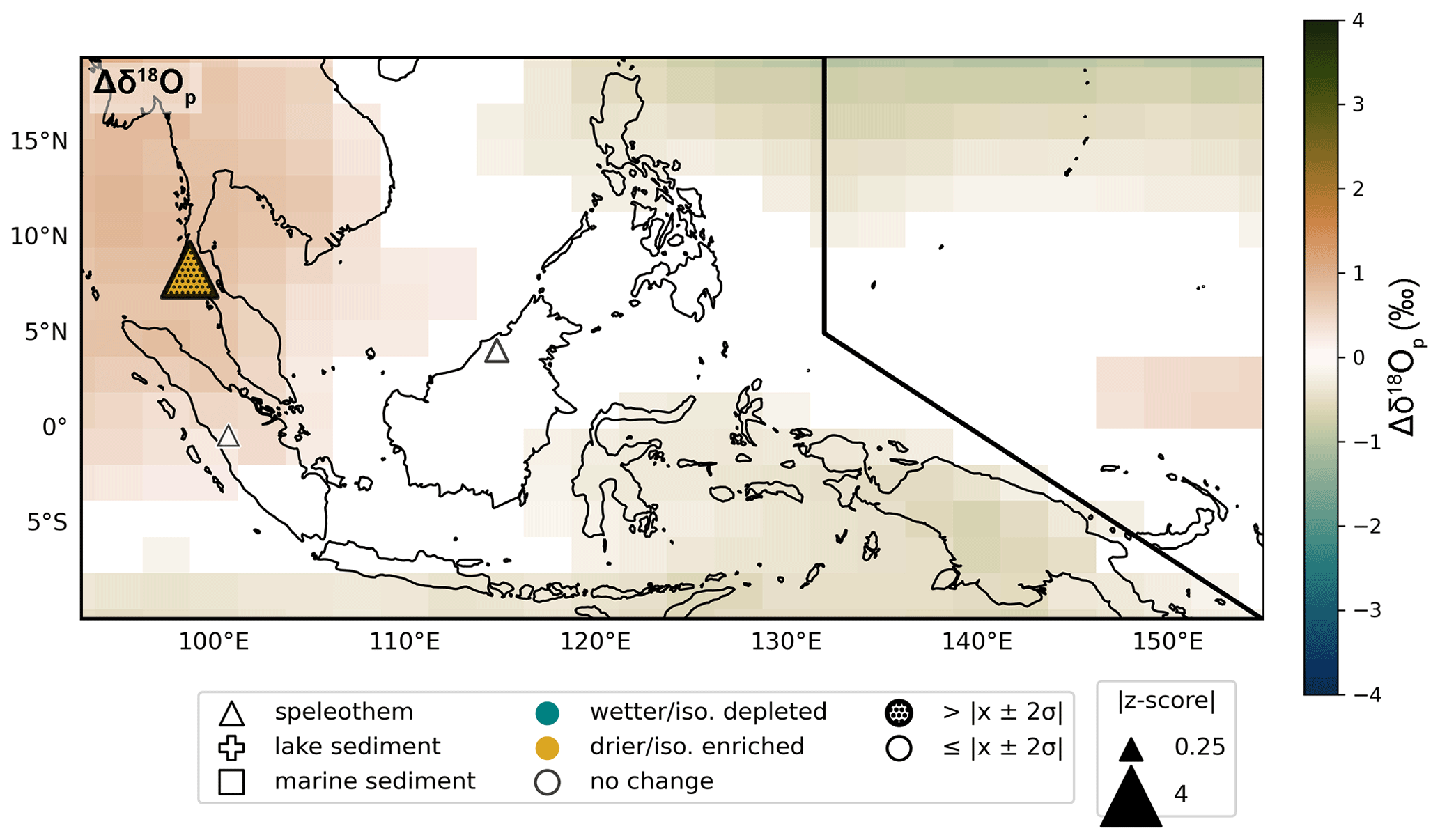
Figure B8 As in Fig. B5, but for IPCC region 38: Southeast Asia.

Appendix C: actR-MM stackplots

C1 Records with wet/depletion events in both actR and MM

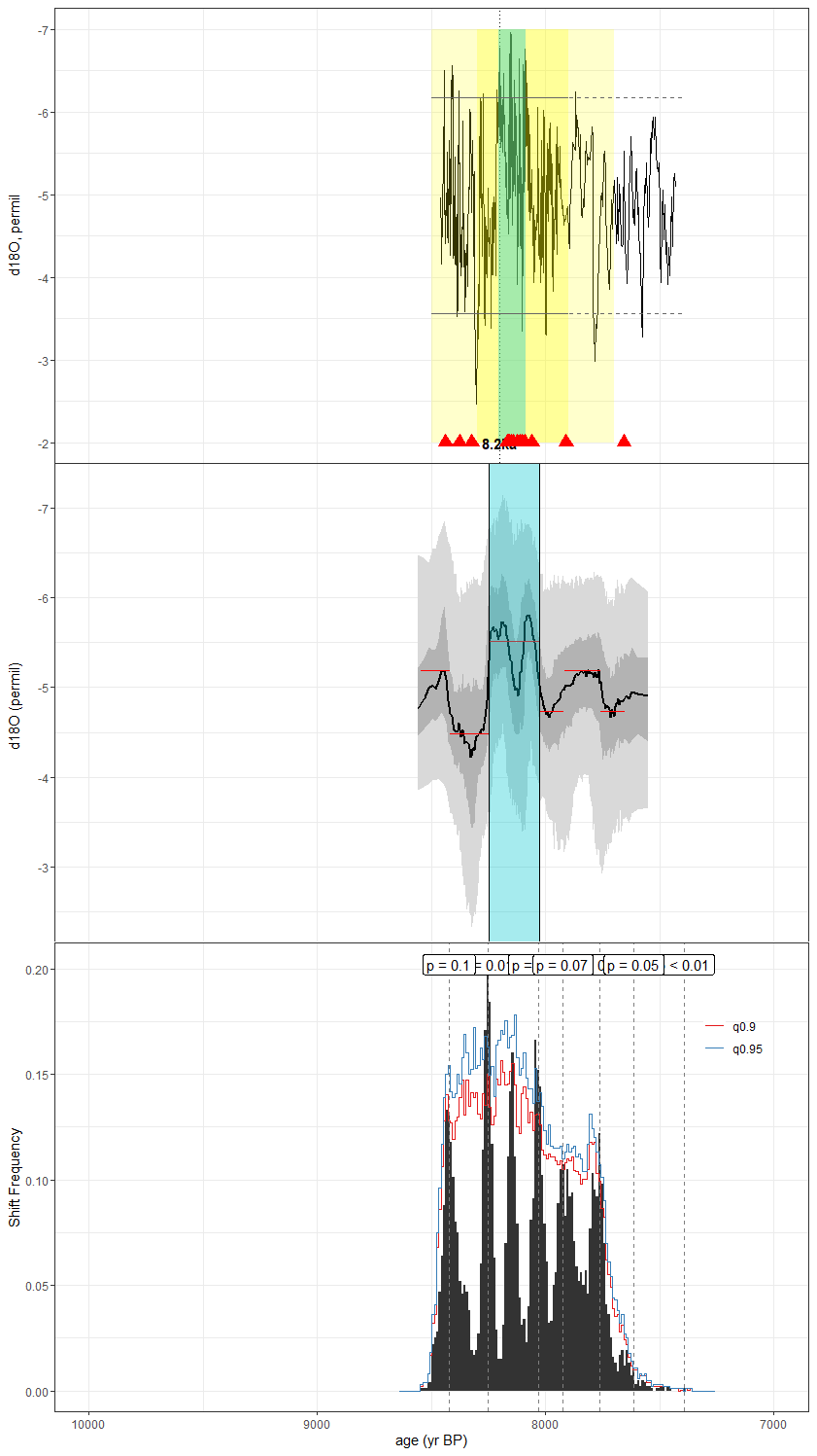
Figure C1 A stackplot from the speleothem record of Duan et al. (2021) (ABC1). The top panel shows the raw oxygen isotope time series with 7.9–8.3 ka highlighted in darker yellow and 7.7–8.5 ka highlighted in lighter yellow, with the ages of radiometric dates represented by red triangles (see schematic in Fig. B1 for more information). The middle panel shows the same time series with age and paleodata ensemble uncertainty quantile ribbons, where the outermost (lighter) bands represent extreme values and the innermost (darker) bands central values. The horizontal red lines represent mean values assigned to the data by actR, with discontinuities indicating significant changepoints. Vertical blue highlights in the top and middle panels indicate “wet” events derived using the MM and actR methods, respectively, with the width of the highlighted area reflecting the duration of the events as calculated from each method. A bold black outline around the highlighted section indicates a “significant” change, while the lack of an outline reflects “tentative” change. For records reflecting “dry” events (as in Fig. B1), these areas are highlighted in brown instead of blue. The lower panel depicts the frequency of shifts detected in the ensemble dataset (black histogram) relative to 100 null hypothesis surrogate datasets. Red and blue histogram lines represent confidence levels at 90 % and 95 %, respectively. Dashed vertical lines give the p-values of detected shifts in mean at the alpha =0.10 level. The age model in the original publication was based on the MOD-AGE algorithm, while the age model used in this synthesis was constructed using the geoChronR package and BACON algorithm.

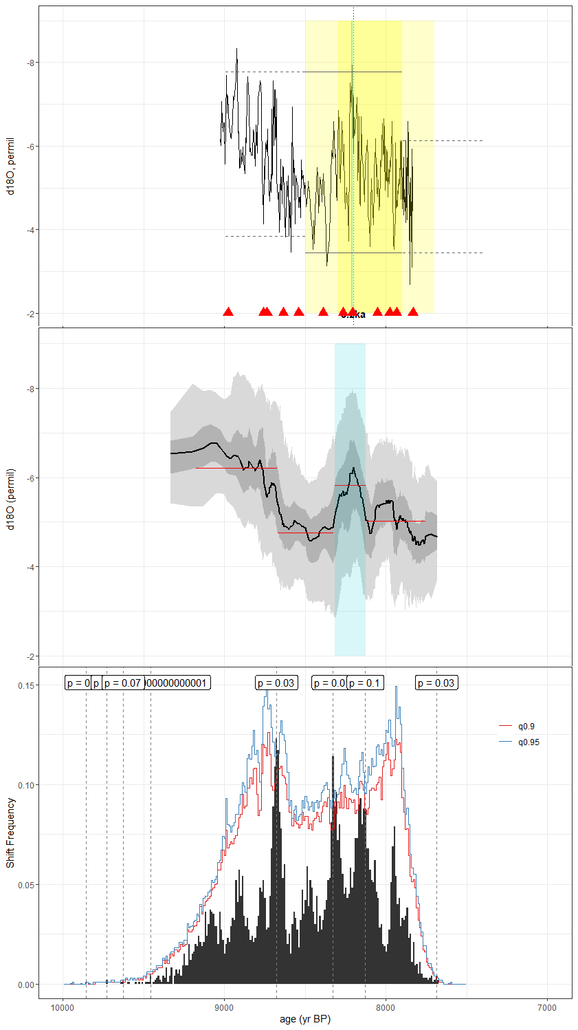
Figure C2 As in Fig. C1, but for the speleothem record of Voarintsoa et al. (2017) (ANJB2). The age model of the original publication was constructed using StalAge. Here, we used the BACON age ensemble from SISALv2.

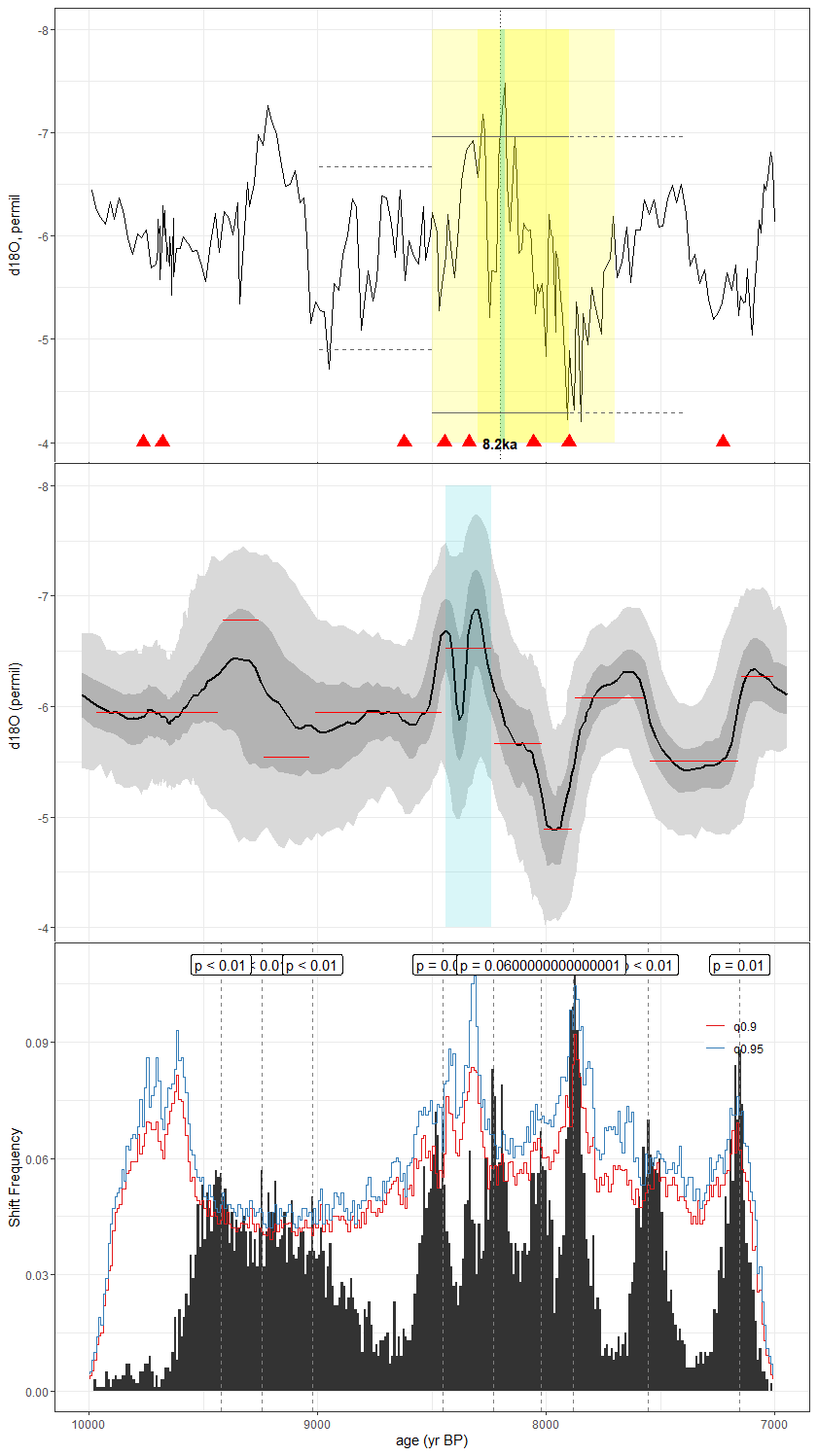
Figure C3 As in Fig. C1, but for the speleothem record of Strikis et al. (2011) (LG11). The original method used in construction of the published age model was unreported, but we leverage the BACON age ensemble published in SISALv2 for our analyses.

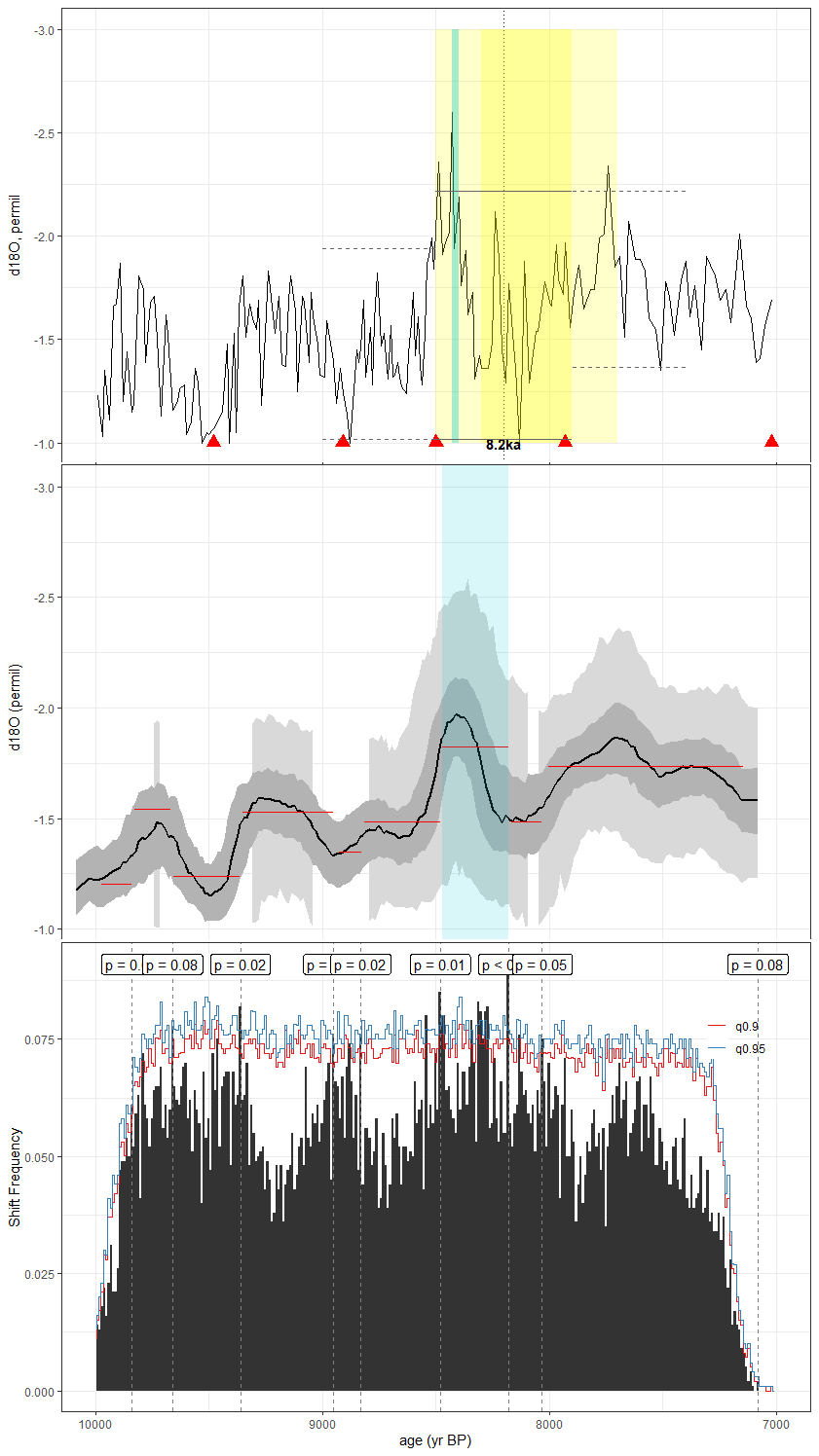
Figure C4 As in Fig. C1, but for the foraminifera record of LoDico et al. (2006) (MD022550). The published age model was constructed using CALIB 5.0, with a 400-year reservoir age correction applied. Here, we used the BACON algorithm included in geoChronR to create the age ensemble.

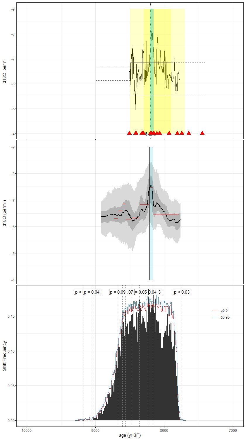
Figure C5 As in Fig. C1, but for the speleothem record of Cheng et al. (2009) (PAD07). The original age modeling method used in the construction of the published time series is unknown. Here, we present an age ensemble using the BACON algorithm provided by geoChronR.

C2 Records with dry/enrichment events in both actR and MM

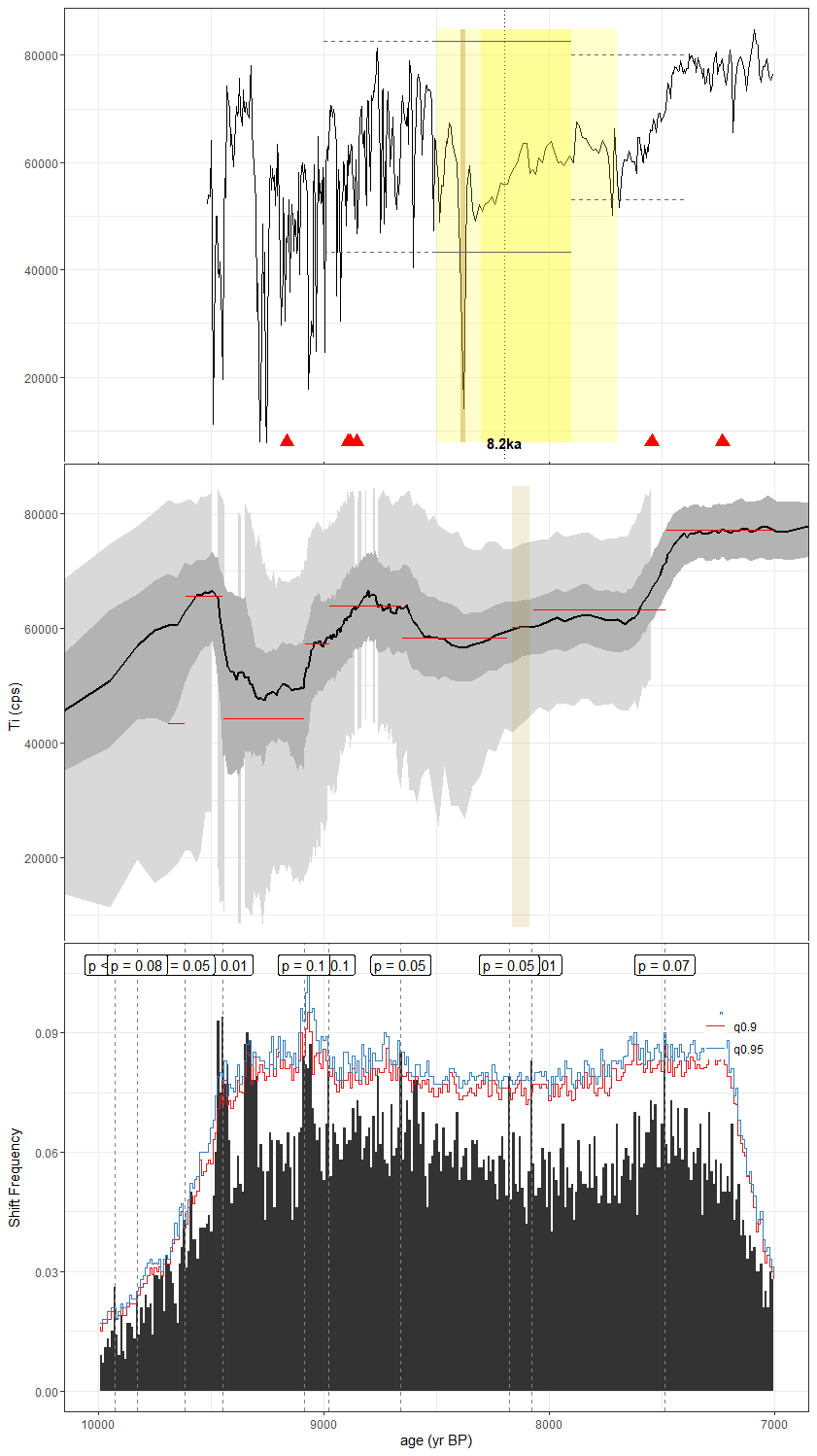
Figure C6 As in Fig. C1, but for the lacustrine titanium content record of Duarte et al. (2021) (Core5LI). The published age model was constructed using BACON using the IntCal20 calibration curve, and here, we construct our age ensemble using the BACON algorithm included with geoChronR.

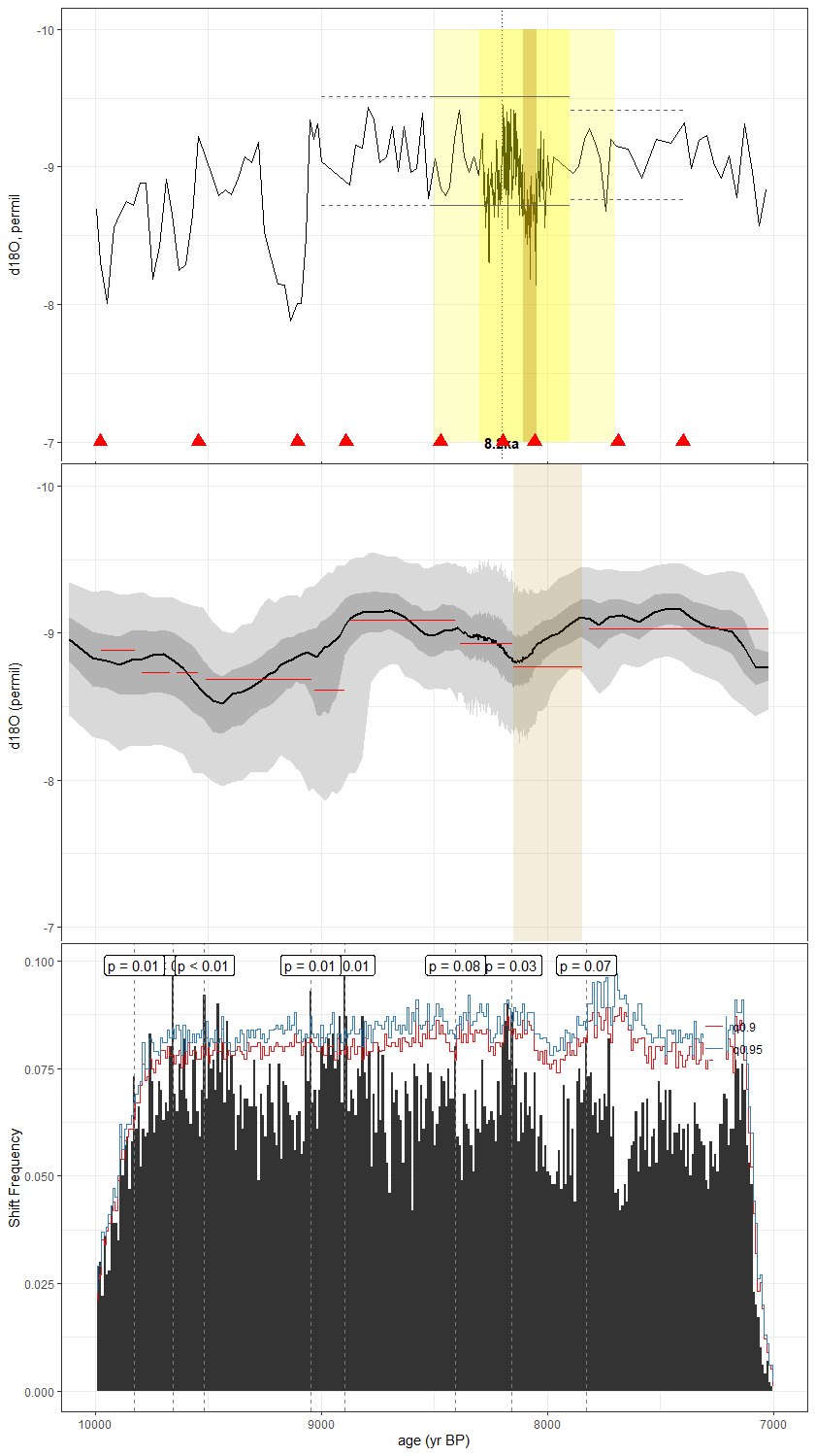
Figure C7 As in Fig. C1, but for the speleothem record of Dykoski et al. (2005) (D4Dykoski). The published age model was constructed by linearly interpolating between U/Th dates. Here, we reconstruct the age model using the BACON algorithm in geoChronR.

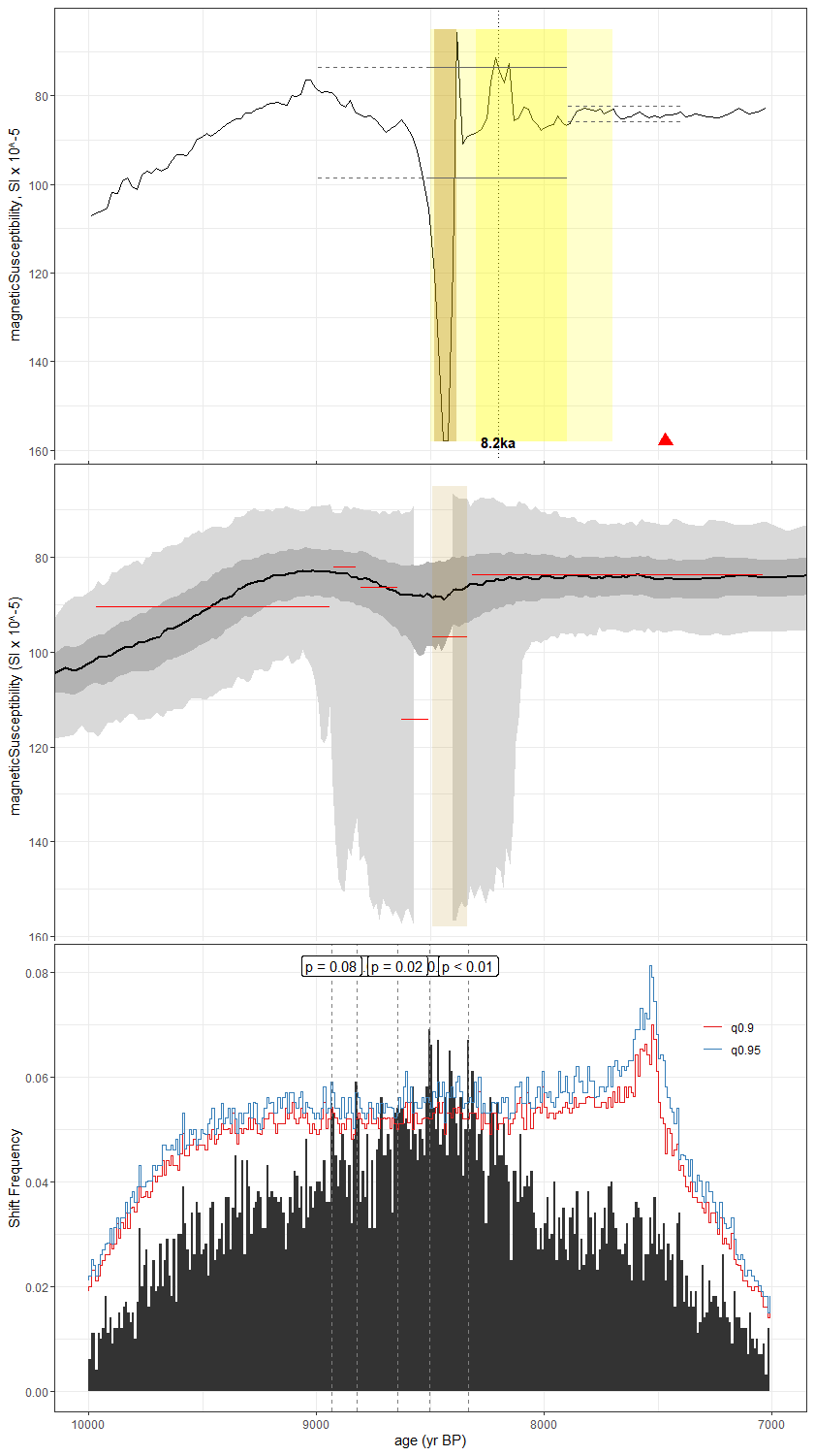
Figure C8 As in Fig. C1, but for the lake sediment magnetic susceptibility record of Hillman et al. (2021) (F14). The original age model was constructed using BACON with the IntCal20 calibration curve. Here, we have reconstructed it using the BACON algorithm in geoChronR.

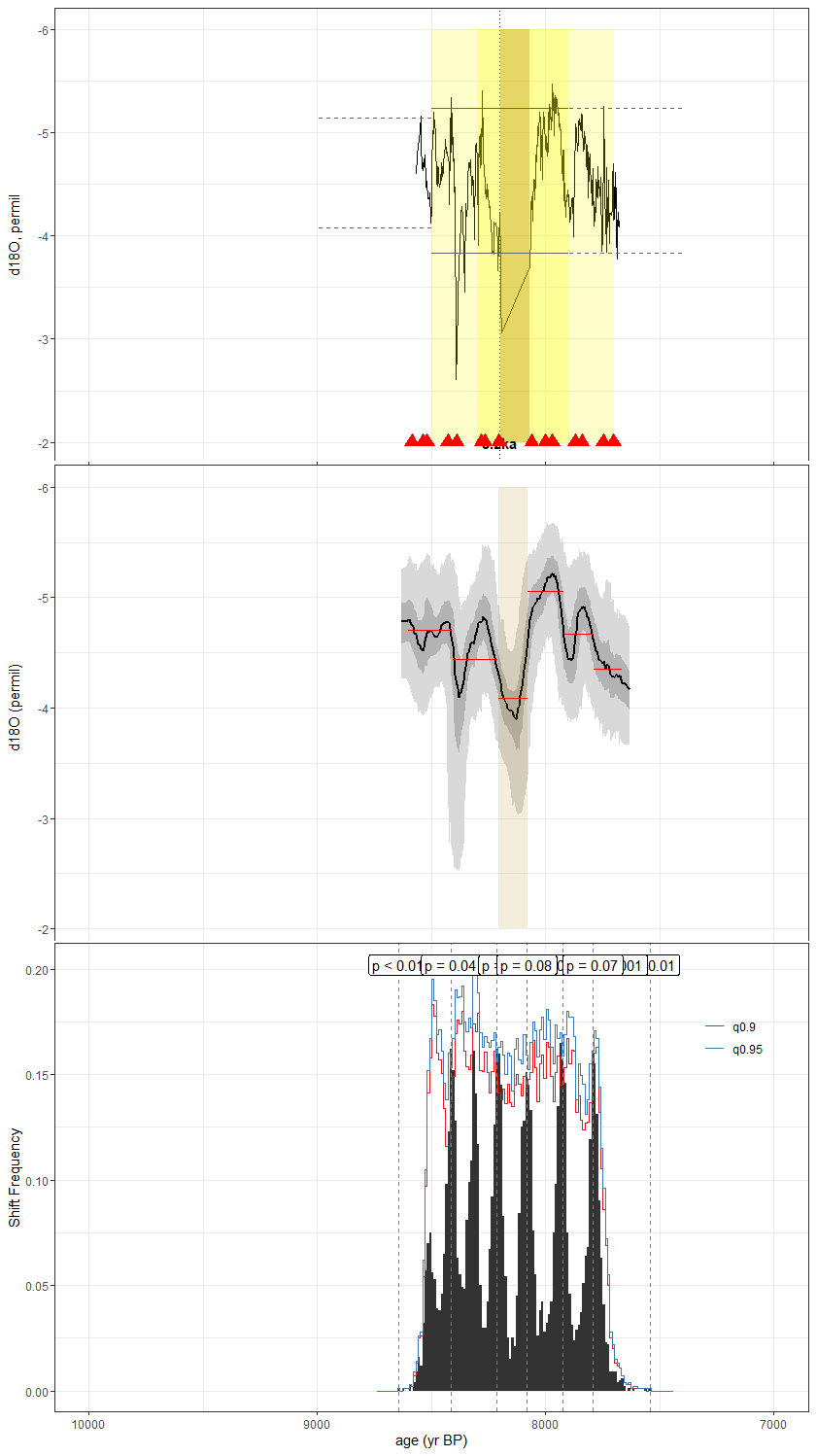
Figure C9 As in Fig. C1, but for the speleothem record of Cheng et al. (2009) (H14). The age modeling algorithm used to construct the original age model was unreported. Here, we constructed our age ensemble using BACON in geoChronR.

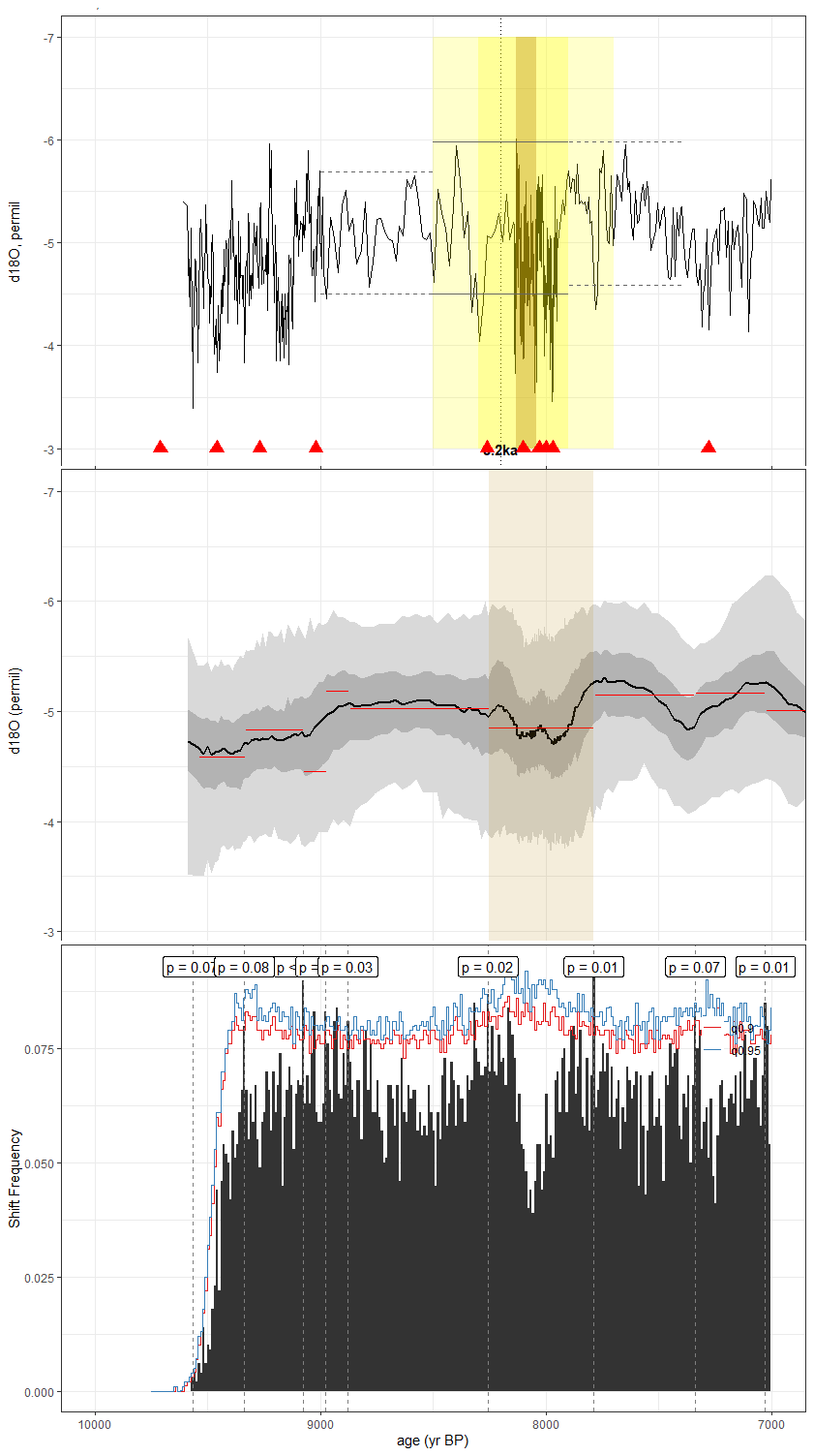
Figure C10 As in Fig. C1, but for the speleothem record of Neff et al. (2001) (H5). While the method used in the construction of the published time series was unreported, we leveraged the SISALv2 BACON ensemble for our analyses.

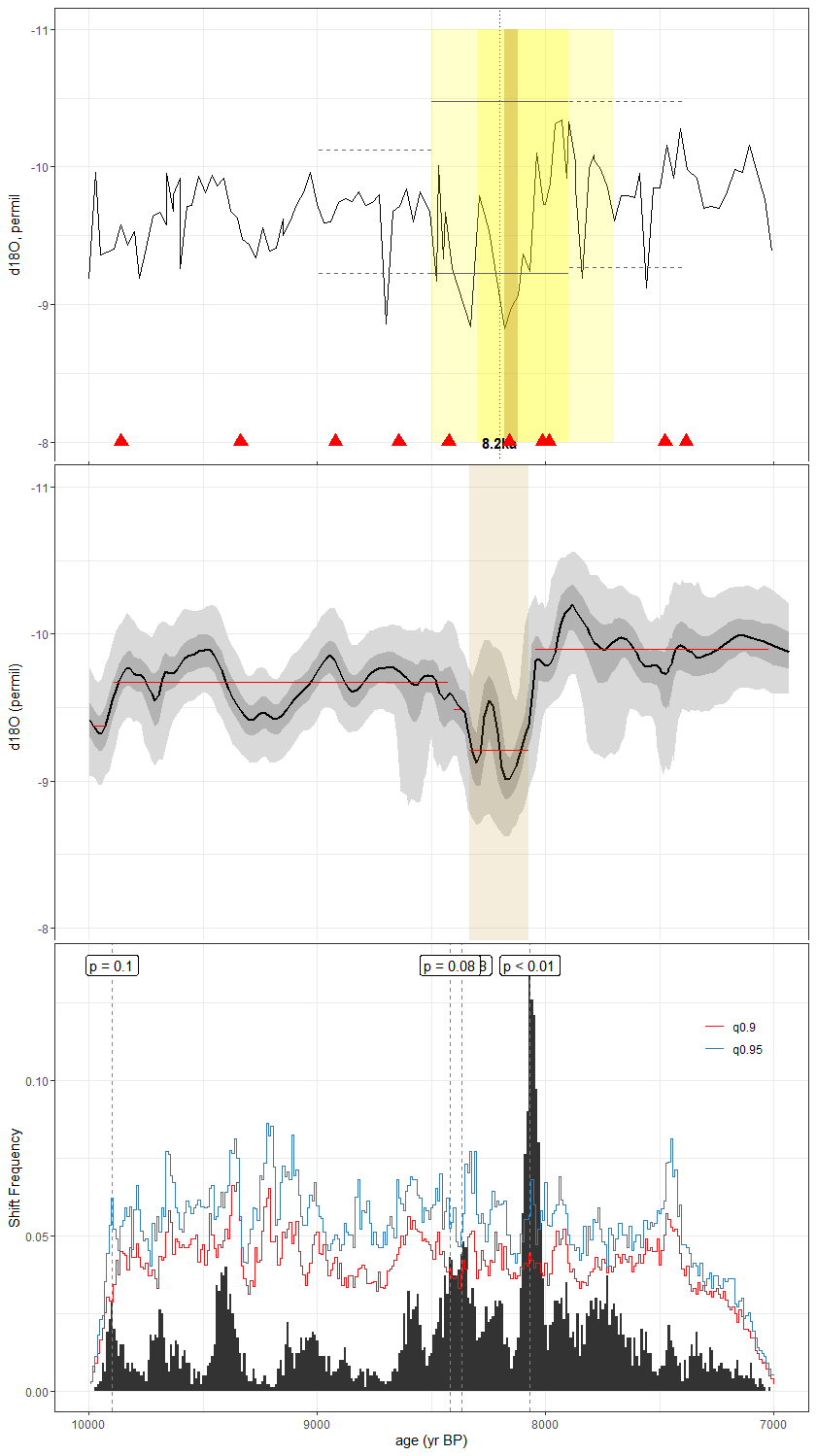
Figure C11 As in Fig. C1, but for the speleothem record of Yang et al. (2019) (HF01). The published age model was constructed via polynomial regression between radiometric dates. For our analyses, we leveraged the copRa age ensemble included in version 2 of the SISAL database.

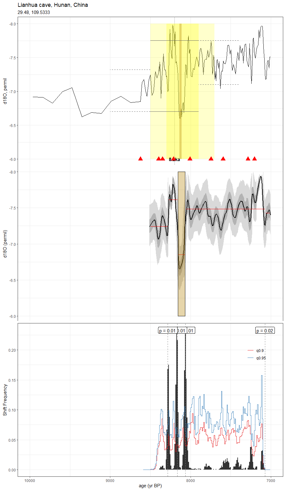
Figure C12 As in Fig. C1, but for the speleothem record of Zhang et al. (2013) (LH2). The published age model was generated by linearly interpolating between radiometric dates. Here, we employ the BACON age ensemble included in version 2 of the SISAL database.

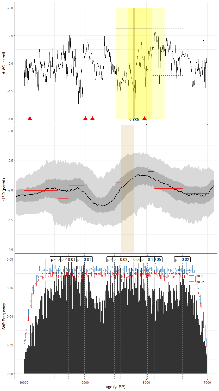
Figure C13 As in Fig. C1, but for the speleothem record of Fleitmann et al. (2007) (Q52007). The published age model was created via a polynomial fit to the age-depth curve of the Th–U data. Our age ensemble leverages the BACON algorithm included in geoChronR.

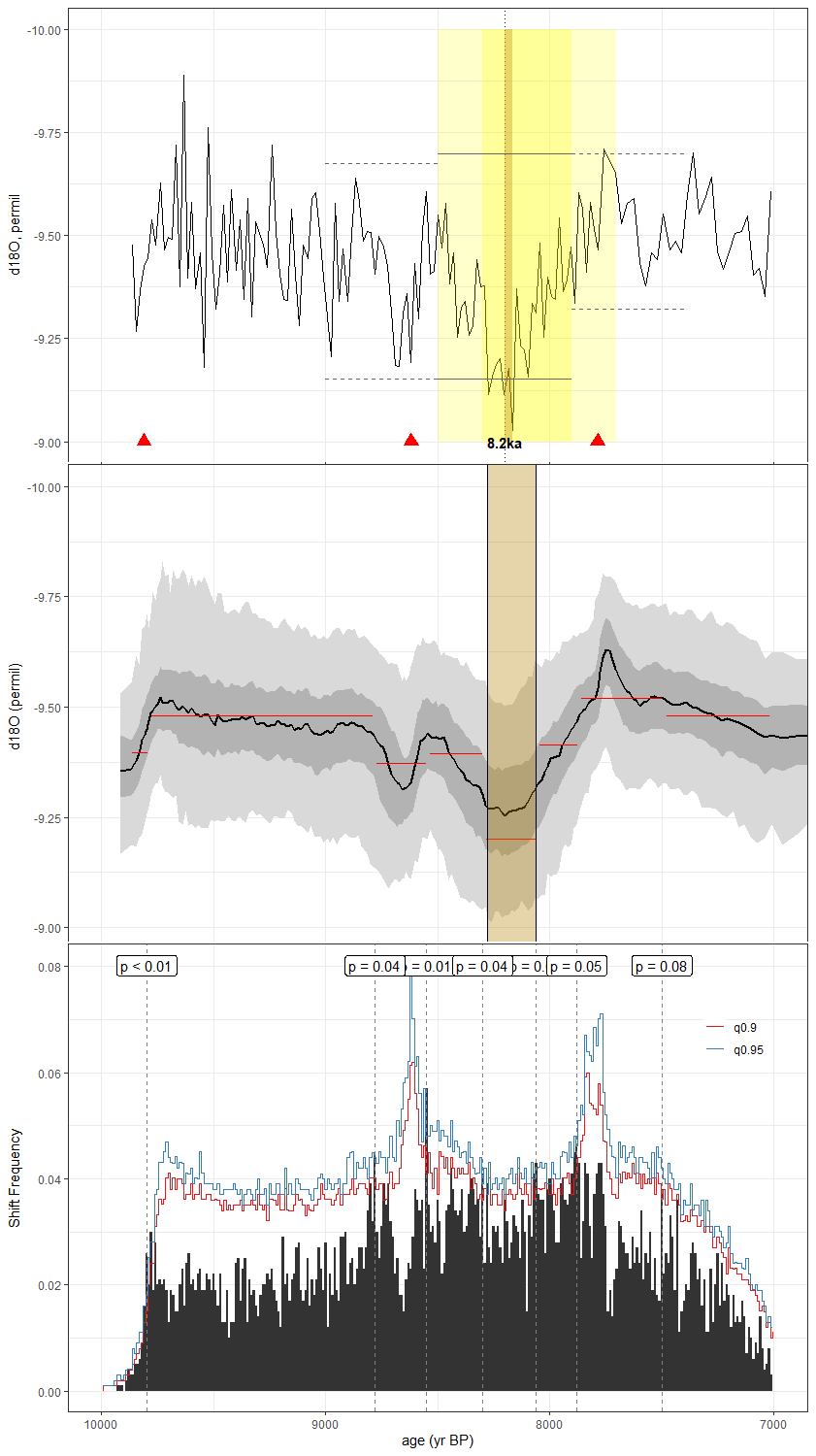
Figure C14 As in Fig. C1, but for the speleothem record of Jiang et al. (2012) (SG1). The published age model was constructed by linear interpolation between U/Th dates. Here, we leverage the BACON ensemble from SISALv2 for our analyses.

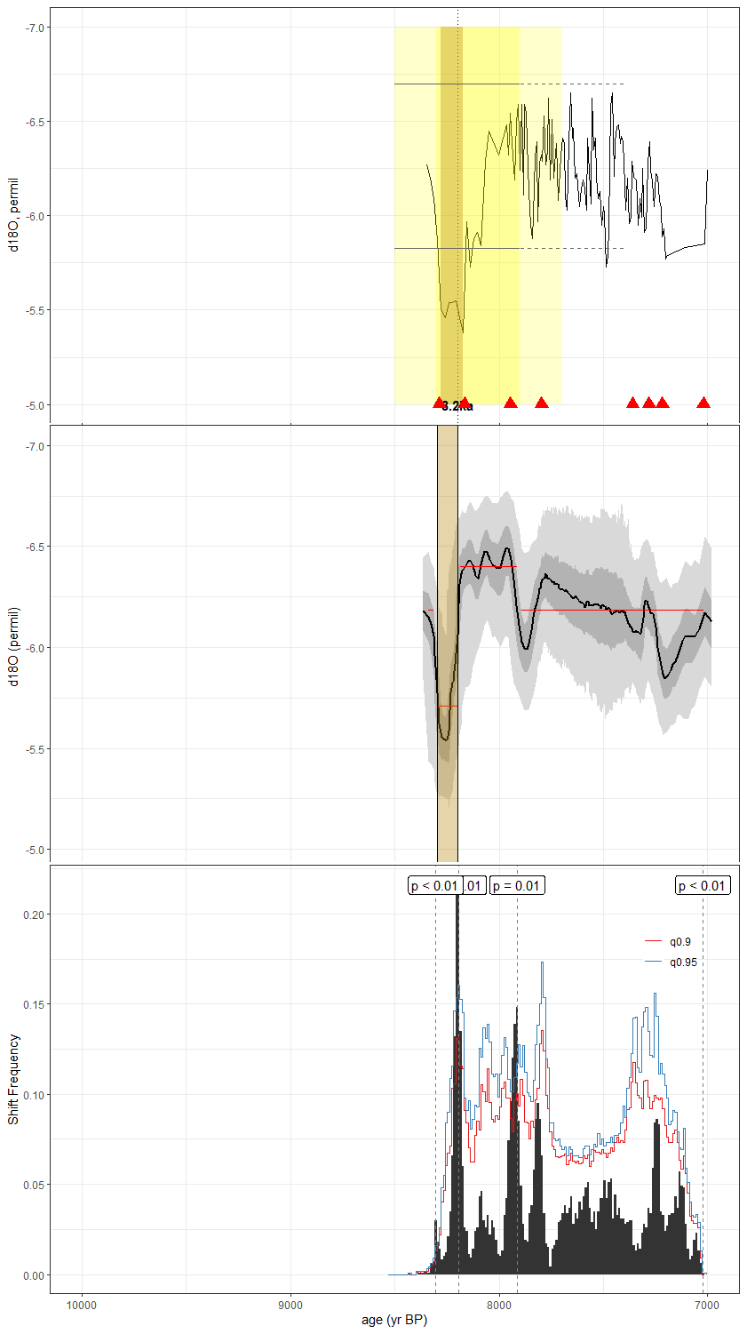
Figure C15 As in Fig. C1, but for the speleothem record of Chawchai et al. (2021) (TK07). The published age model was constructed using the BACON algorithm. Here, we used the BACON age ensemble supplied in the SISALv2 database.

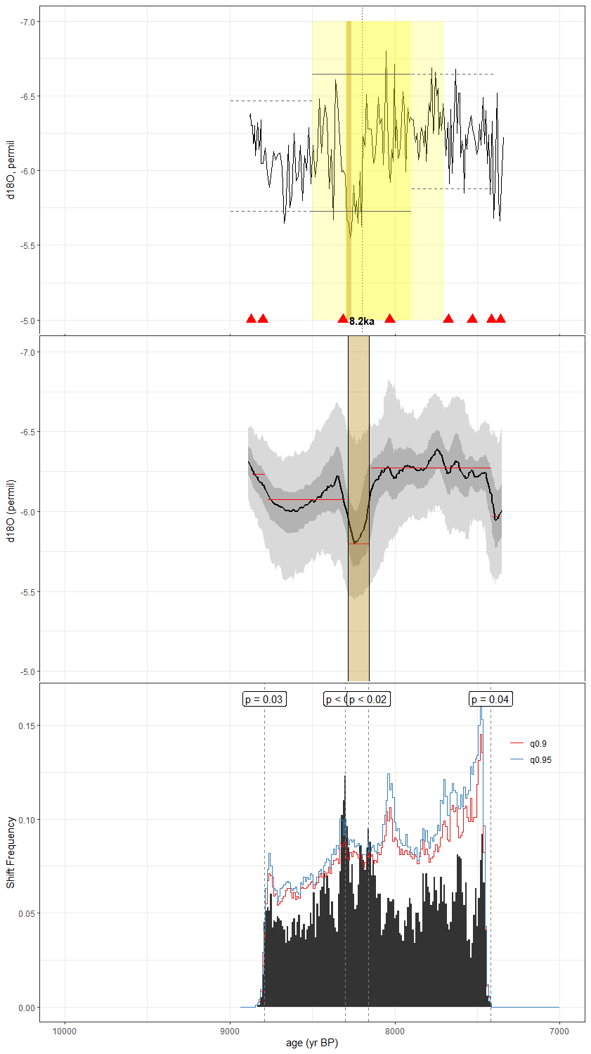
Figure C16 As in Fig. C1, but for the speleothem record of Chawchai et al. (2021) (TK20). The published age model was constructed using the BACON algorithm. Here, we used the BACON age ensemble supplied in the SISALv2 database.

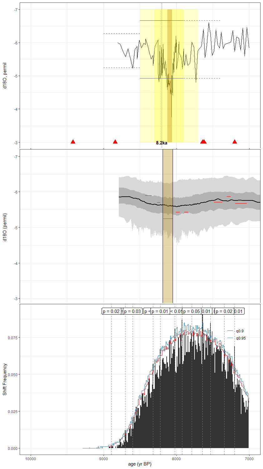
Figure C17 As in Fig. C1, but for the speleothem record of Lachniet et al. (2004) (V1). The published time series was aligned to a fifth-order polynomial best-fit age model between isochron dates. We employ the BACON ensemble provided by SISALv2 for our analyses.

Figure C18 As in Fig. C1, but for the speleothem record of Huang et al. (2016) (ZLP1). The published age model was derived from linear interpolation between radiometric dates. For our analyses, we leveraged the SISALv2 BACON age ensemble.

C3 Records with no event in both actR and MM

Figure C19 As in Fig. C1, but for the lacustrine calcite raft record of Sullivan et al. (2021) (C7). The published age model was constructed using the BACON algorithm and the IntCal13 calibration curve. Here, we reconstruct the BACON age ensemble using geoChronR and the IntCal20 calibration curve.

Figure C20 As in Fig. C1, but for the lacustrine gastropod δ¹⁸O record of Curtis et al. (1998) (Curtis6VII93). The published age model was constructed by linearly interpolating between ¹⁴C dates derived from terrestrial wood and charcoal samples. Here, we construct the age ensemble using the BACON algorithm included in geoChronR.

Figure C21 As in Fig. C1, but for the speleothem record of Li et al. (2011) (FR5). The age modeling algorithm used to construct the original age model was unreported, but leveraged the IntCal09 calibration curve. Here, we use the copRa age ensemble included in SISALv2.

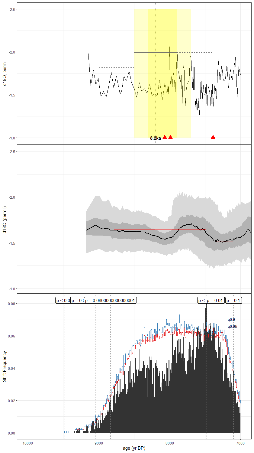
Figure C22 As in Fig. C1, but for the foraminifera record of Schmidt et al. (2012) (JPC51). The published age model was created using CALIB 6.0, with a standard −400-year reservoir age correction for surface waters. Here, we use the BACON algorithm included in geoChronR to produce our age ensemble.

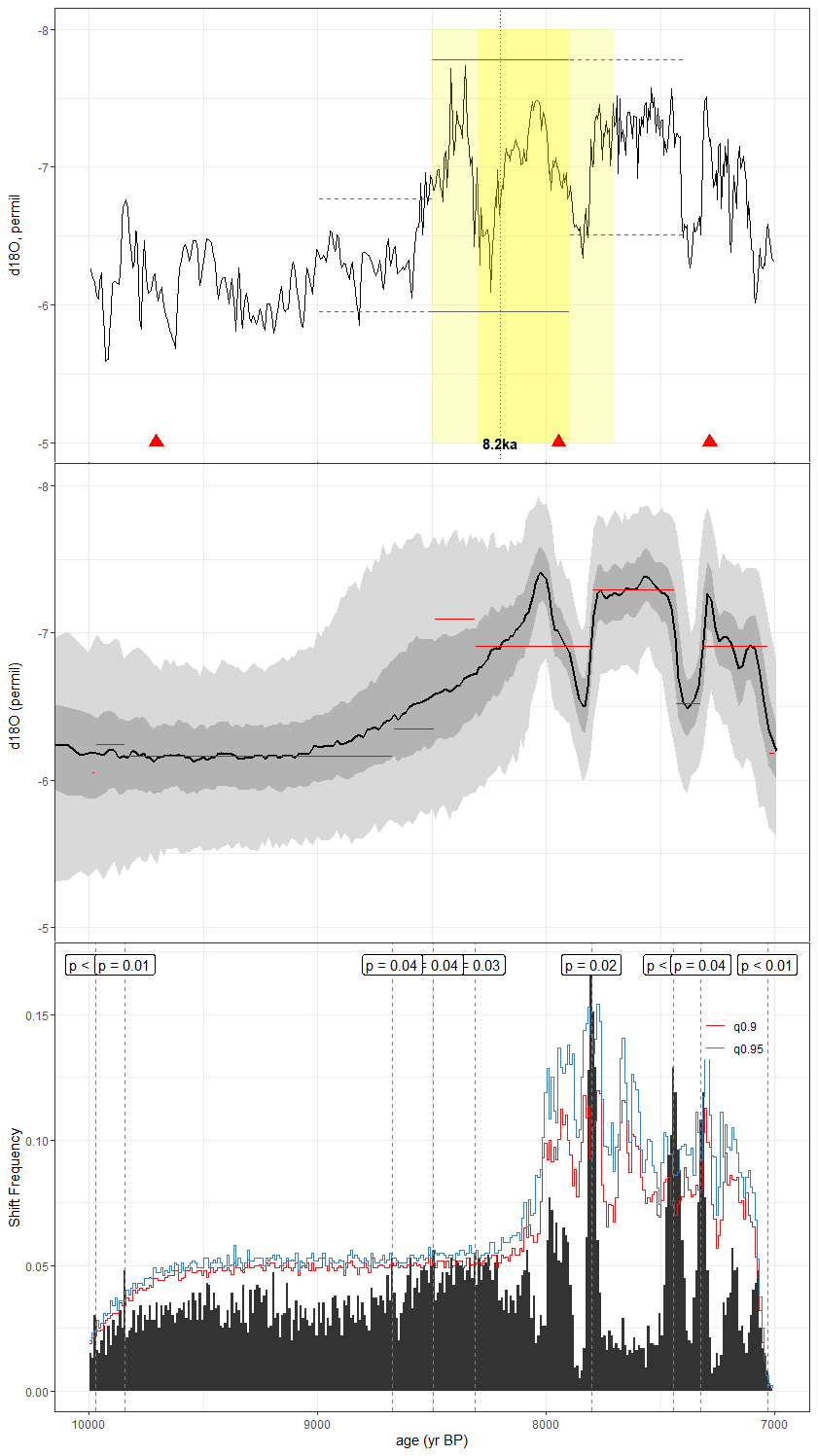
Figure C23 As in Fig. C1, but for the speleothem record of Berkelhammer et al. (2013) (KMA). The published age model was created using the StalAge algorithm. Here, we used the BACON age ensemble included in SISALv2.

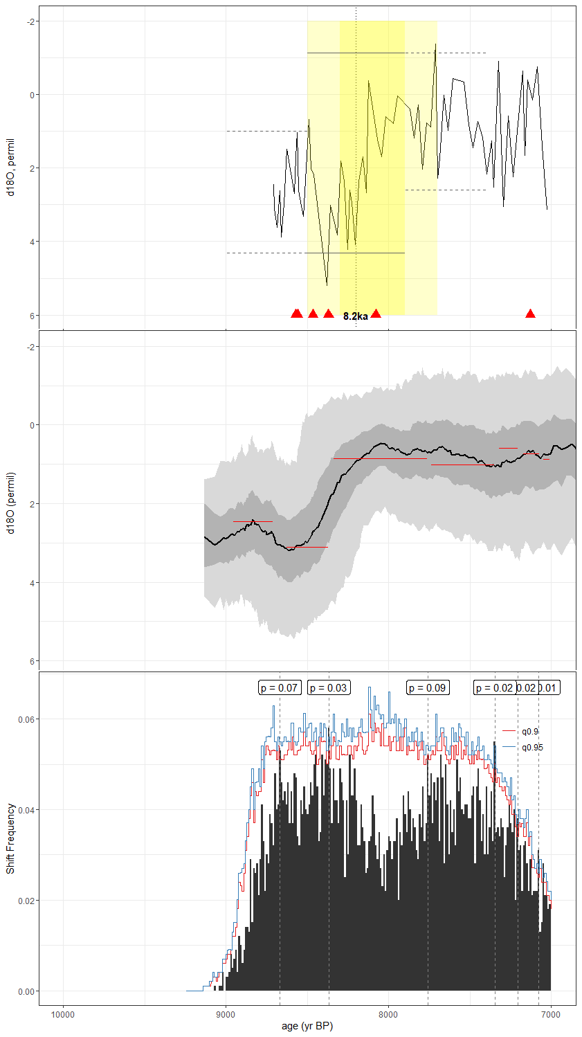
Figure C24 As in Fig. C1, but for the lake sediment δ¹⁸O record of Wahl et al. (2014) (LagoPuertoArturo). The published age model was constructed using CLAM 2.2 and the IntCal13 calibration curve. For our analyses, we reconstructed the age model using BACON and IntCal20 in geoChronR.

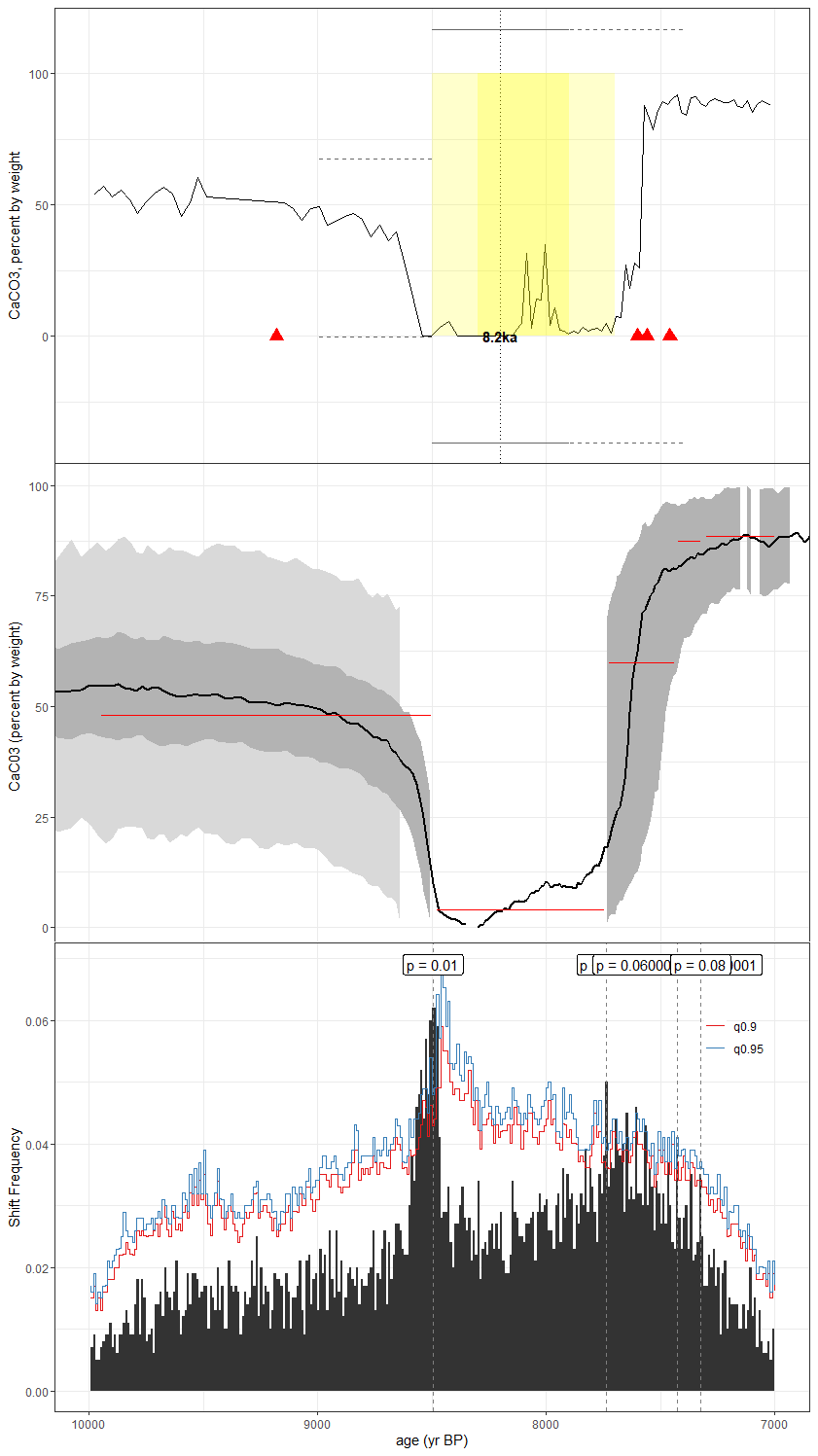
Figure C25 As in Fig. C1, but for the lake sediment record of Hodell et al. (1995) (LC1). The published age model was created using the decadal tree ring dataset in CALIB. Here, we use BACON with the IntCal20 calibration curve supplied by geoChronR.

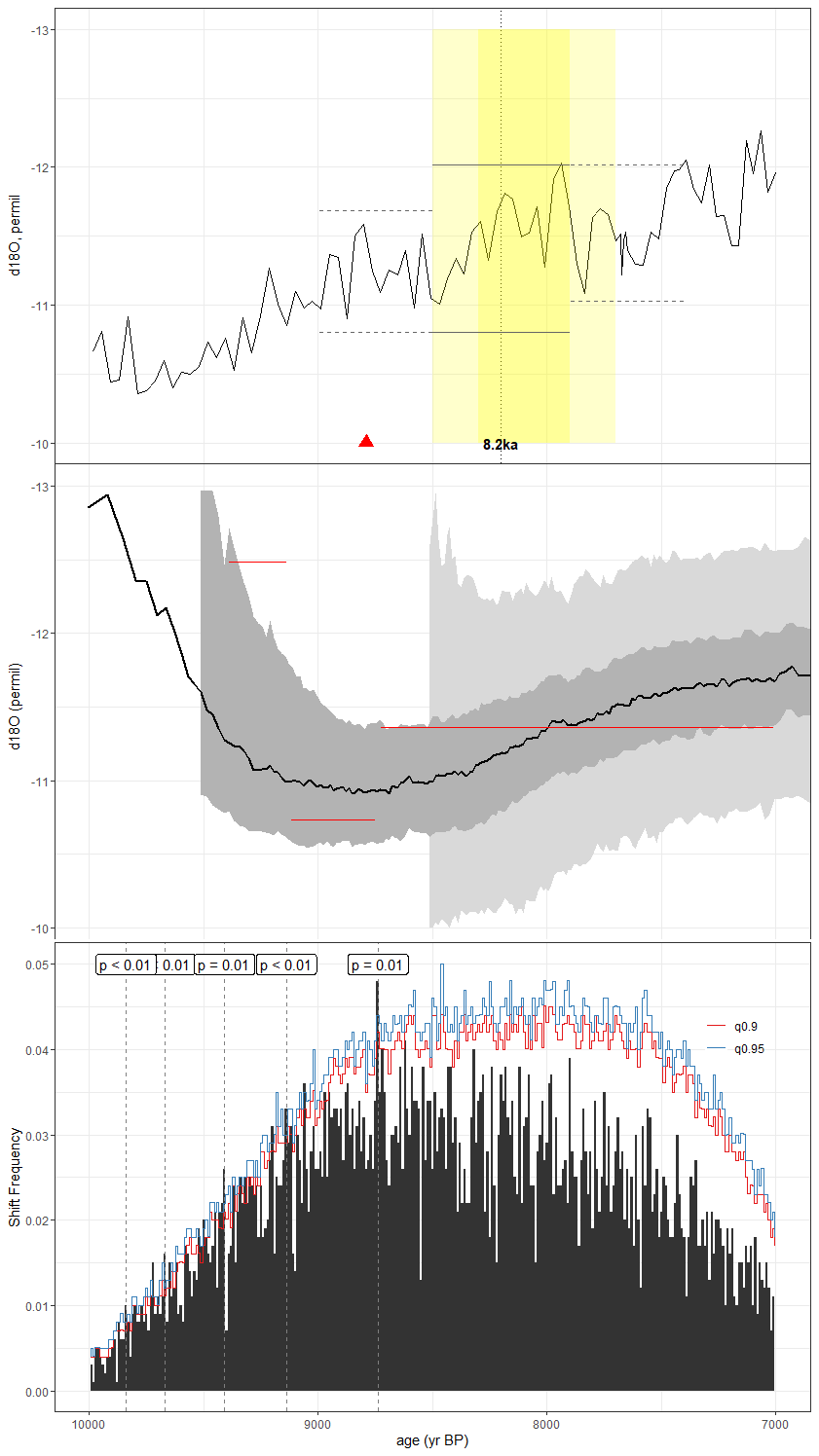
Figure C26 As in Fig. C1, but for the lacustrine sediment record of Bird et al. (2011) (LP). The published age model was created using CALIB 5.0 with an unreported calibration curve. Here, we construct our age ensemble in geoChronR using the BACON algorithm and SHCal20.

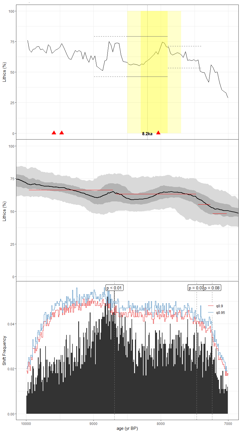
Figure C27 As in Fig. C1, but for the lake sediment (percent lithics) record of Bird et al. (2014) (ParuCo). CALIB 6.0 and the IntCal09 calibration curve were used in the construction of the published age model. We construct our age ensemble using BACON and IntCal20 via geoChronR.

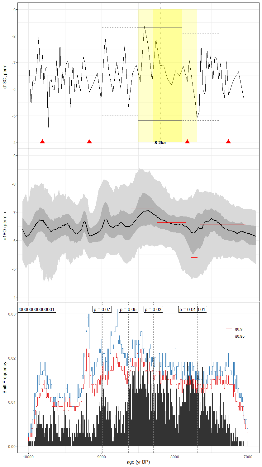
Figure C28 As in Fig. C1, but for the speleothem record of Cruz et al. (2009) (RN1). The method used in the construction of the published age model was unreported, but we leverage the Bchron ensemble supplied in version 2 of the SISAL database for our analyses.

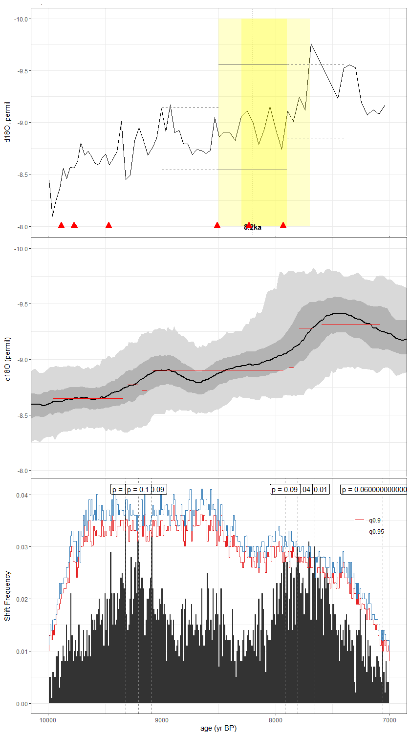
Figure C29 As in Fig. C1, but for the speleothem record of Carolin et al. (2016) (SSC01). StalAge was used to construct the published age model. We used the BACON algorithm included in geoChronR to generate our age ensemble.

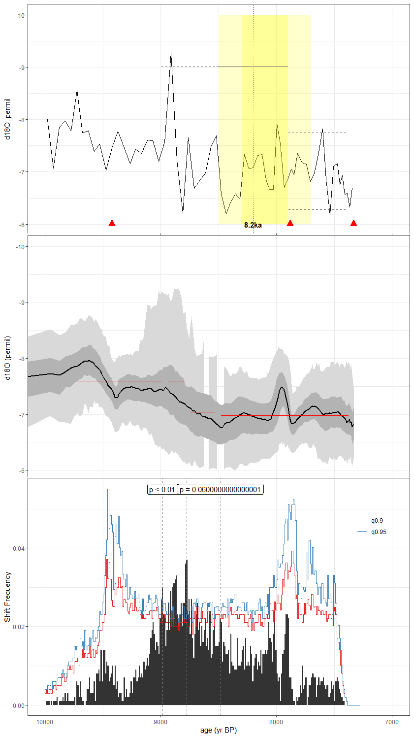
Figure C30 As in Fig. C1, but for the speleothem record of Ward et al. (2019) (TM6). The published age model was constructed using the copRa algorithm, though we use the BACON age ensemble supplied in the SISALv2 database for our analyses.

C4 Records with conflicting signals in actR and MM

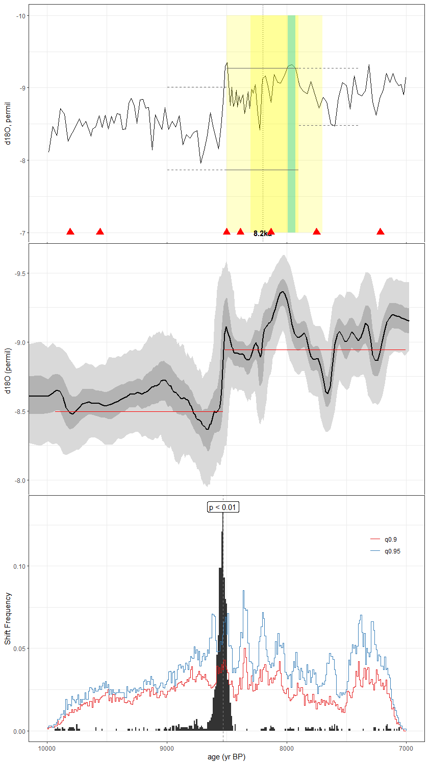
Figure C31 As in Fig. C1, but for the speleothem record of Chen et al. (2016) (BA03). The published age model was based on the StalAge algorithm, but here, we use the BACON ensemble from SISALv2.

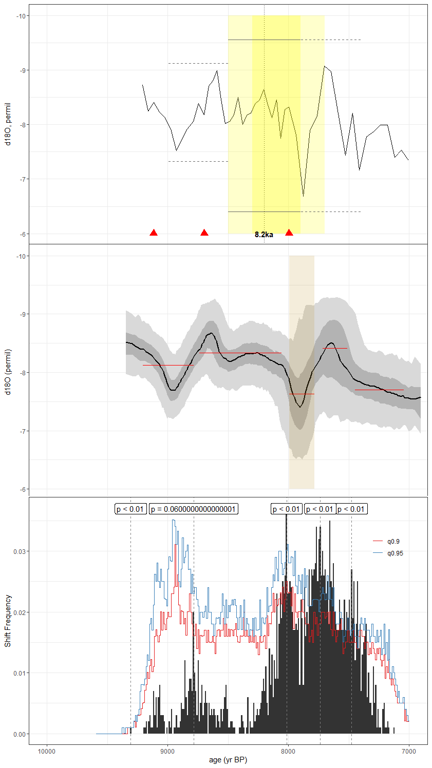
Figure C32 As in Fig. C1, but for the speleothem record of Bernal et al. (2016) (BTV21a). Information about the published age model was unreported. Here, we use the SISALv2 BACON age ensemble.

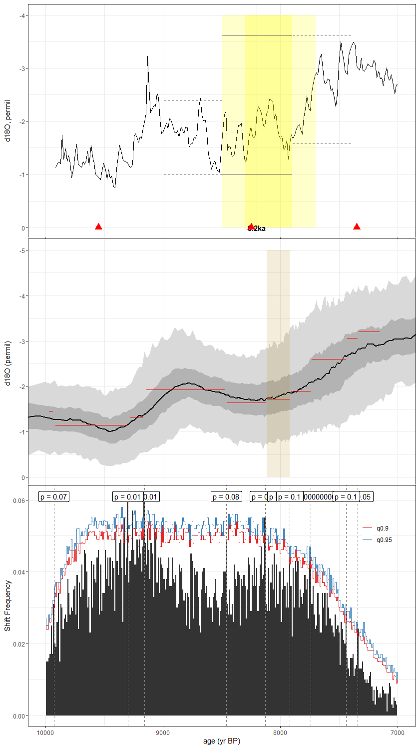
Figure C33 As in Fig. C1, but for the speleothem record of Fensterer et al. (2013) (CM2013). The published age model was constructed using the StalAge algorithm. Here, we use the SISALv2 copRa age ensemble.

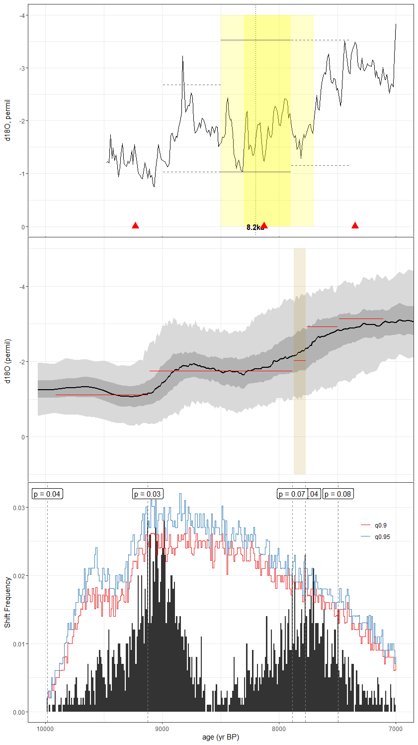
Figure C34 As in Fig. C1, but for the speleothem record of Warken et al. (2019) (CM2019). The published age model was constructed using the StalAge algorithm. Here, we use the SISALv2 BACON age ensemble.

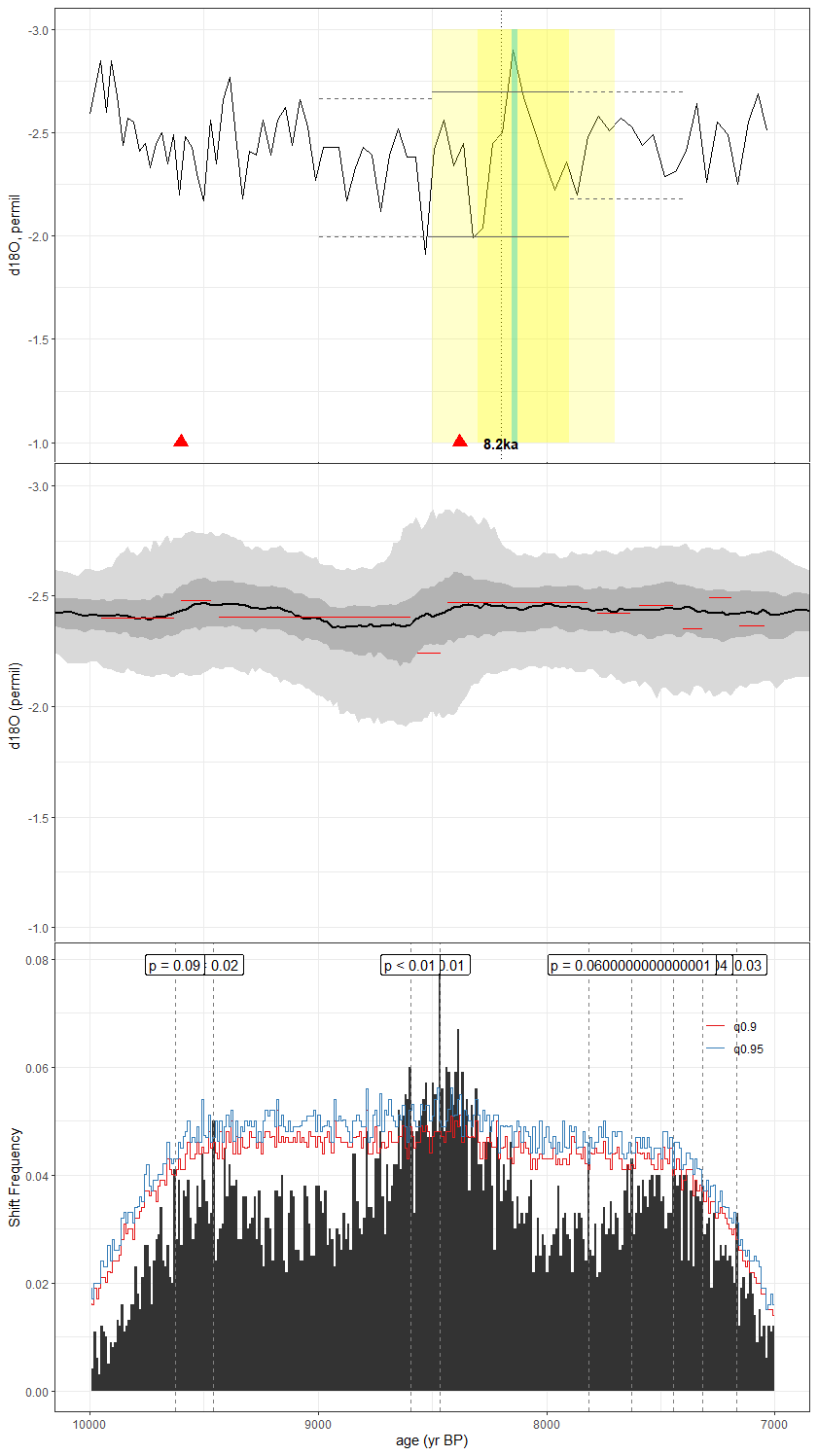
Figure C35 As in Fig. C1, but for the foraminifera record of Wang et al. (1999) (Core17940). The published age model was constructed using CALIB 3.0.3, corrected for a 400-year reservoir age and unspecified calibration curve. We constructed our age ensemble using the BACON algorithm included in geoChronR using the IntCal20 calibration curve.

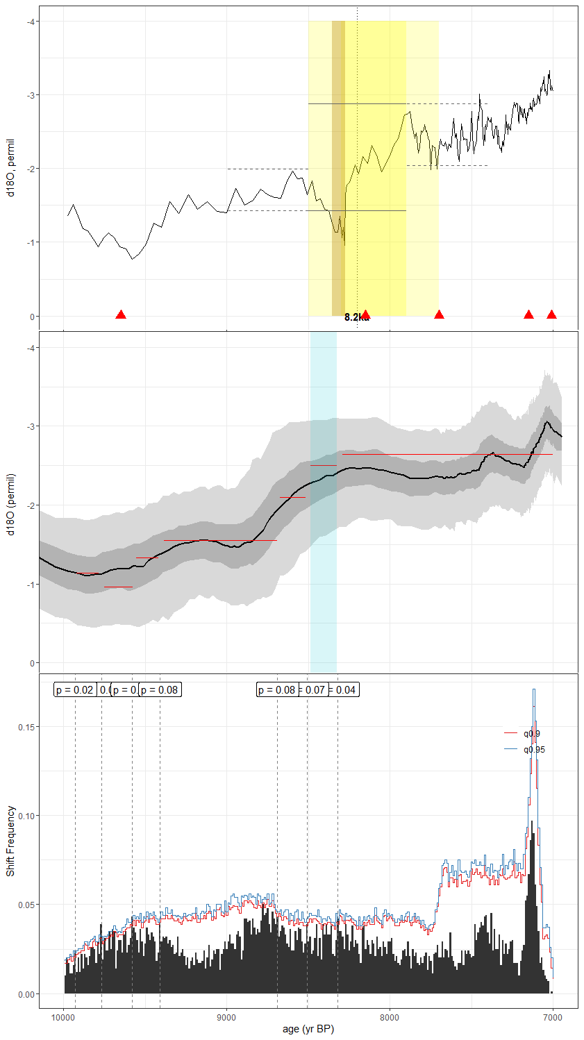
Figure C36 As in Fig. C1, but for the speleothem record of Fensterer et al. (2013) (CP). The published age model was constructed using the StalAge algorithm. We use the Bchron age ensemble constructed in SISALv2 here.

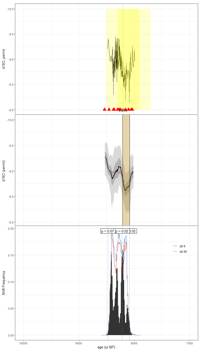
Figure C37 As in Fig. C1, but for the speleothem record of Cheng et al. (2009) (D4Cheng). The age model used in the original publication was unreported. Here, we use the BACON algorithm included in geoChronR to produce our age ensemble.

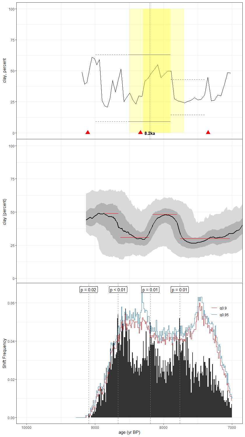
Figure C38 As in Fig. C1, but for the lacustrine clay content record of Conroy et al. (2008) (EJConroy). The published age model was constructed using CALIB 5.0 with the Southern Hemisphere dataset. The age ensemble presented here was created using the BACON algorithm with the SHCal20 calibration curve in geoChronR.

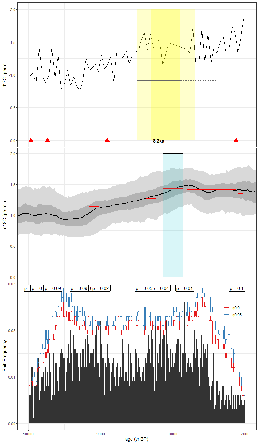
Figure C39 As in Fig. C1, but for the foraminifera record of Thirumalai et al. (2021) (GB2GC1). The published age model was developed using the BACON algorithm and Marine13 calibration curve, which we reconstructed using geoChronR.

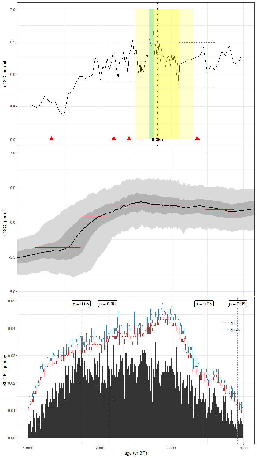
Figure C40 As in Fig. C1, but for the speleothem record of Winter et al. (2020) (GURM1). The published age model was constructed using the copRa algorithm, while we use the BACON ensemble produced for SISALv2 here.

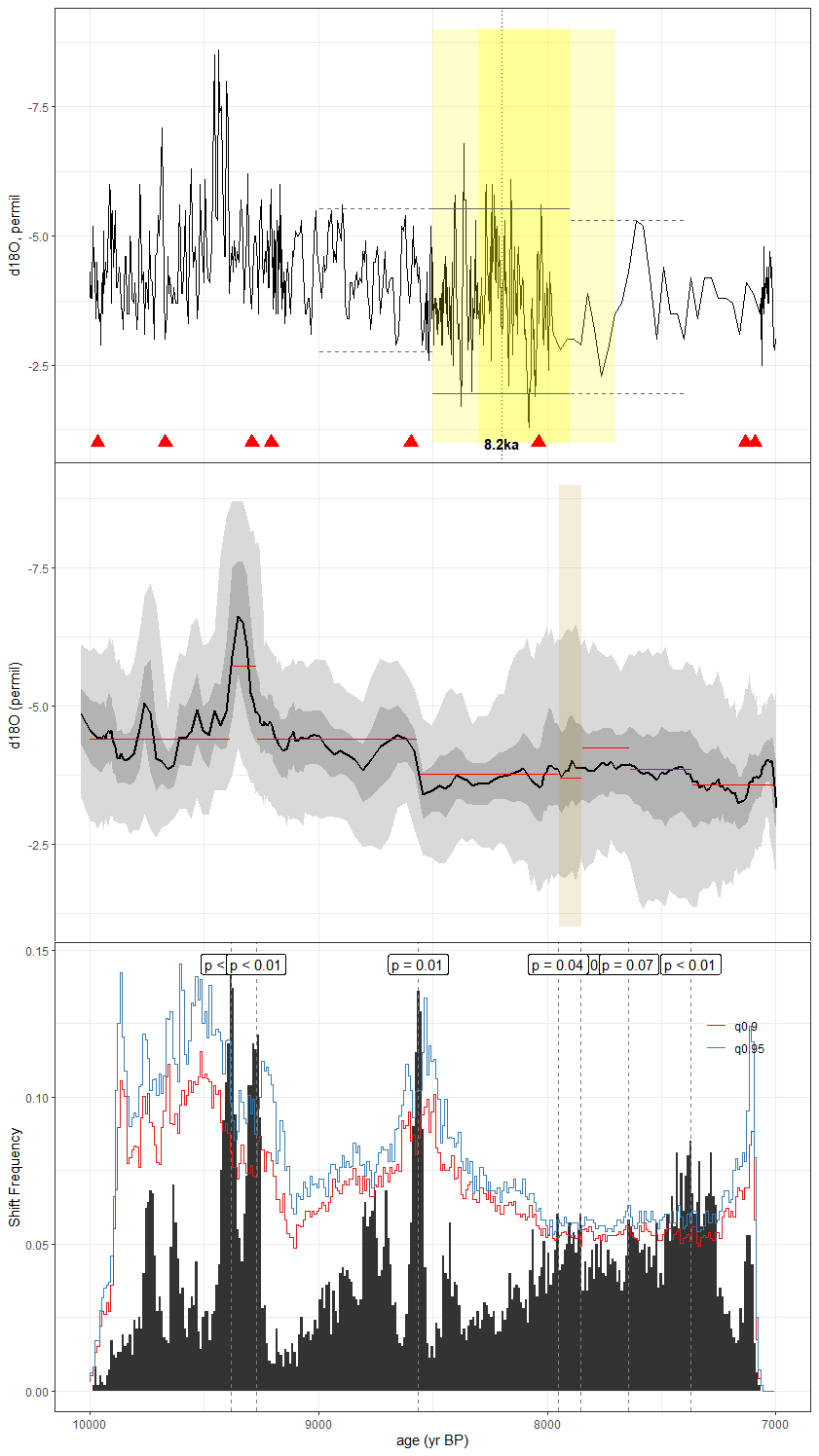
Figure C41 As in Fig. C1, but for the speleothem record of Novello et al. (2017) (JAR7). The published age model was constructed via linear interpolation between radiometric dates. For our analyses, we leveraged the BACON age ensemble produced for SISALv2.

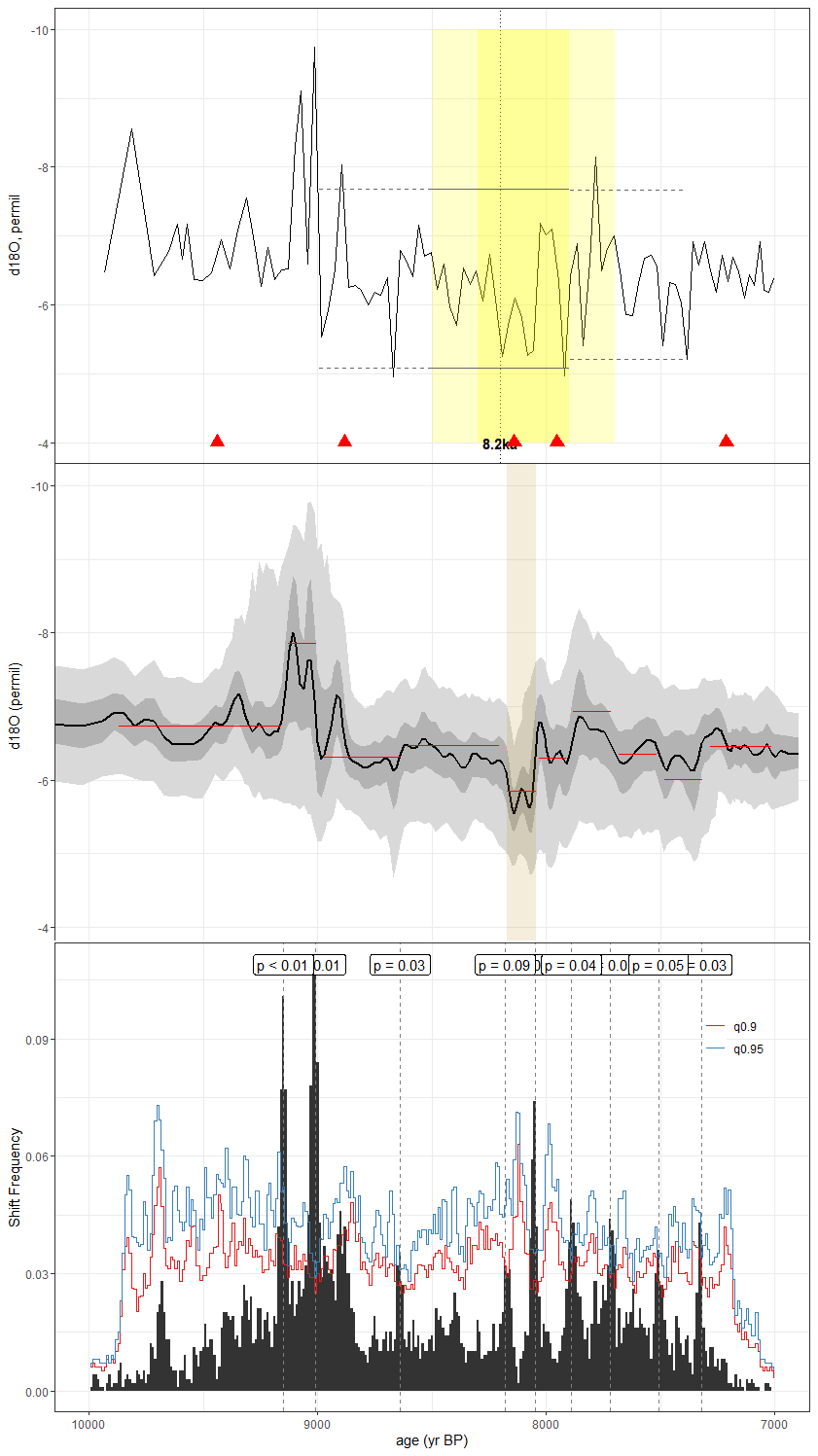
Figure C42 As in Fig. C1, but for the speleothem record of Huguet et al. (2018) (KM1). While the published age model was constructed using the StalAge algorithm, we leverage the Bchron age ensemble included in SISALv2 here.

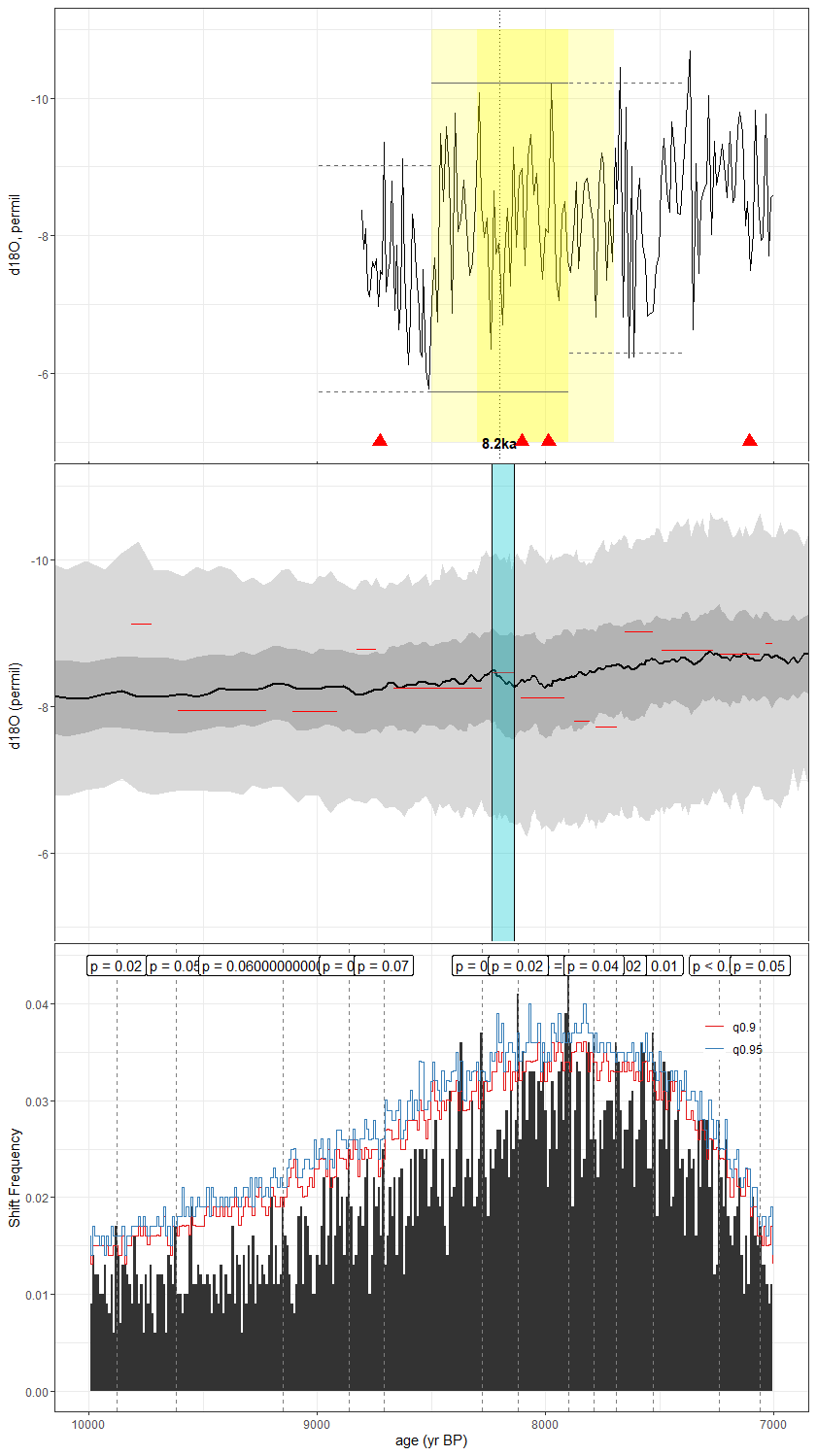
Figure C43 As in Fig. C1, but for the speleothem record of Denniston et al. (2013) (KN51). The method used in the construction of the published age model is unknown, but we use the copRa ensemble generated for SISALv2 here.

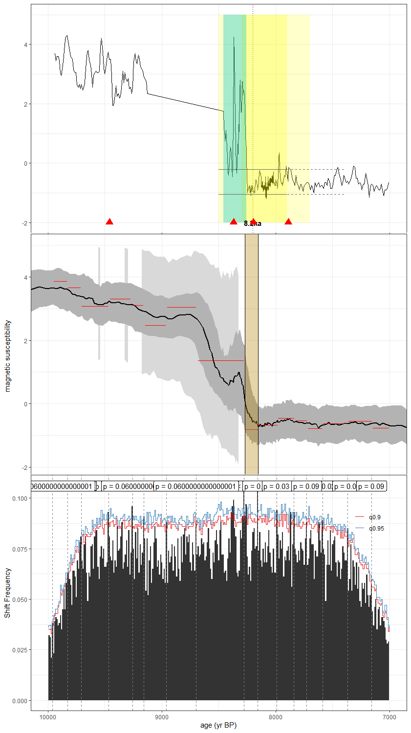
Figure C44 As in Fig. C1, but for the lake sediment magnetic susceptibility record of Polissar et al. (2013) (LBA99). The published age model was constructed by linearly interpolating between radiometric dates with the IntCal04 calibration curve. Here, we constructed our ensemble using the BACON algorithm and IntCal20 curve included in geoChronR.

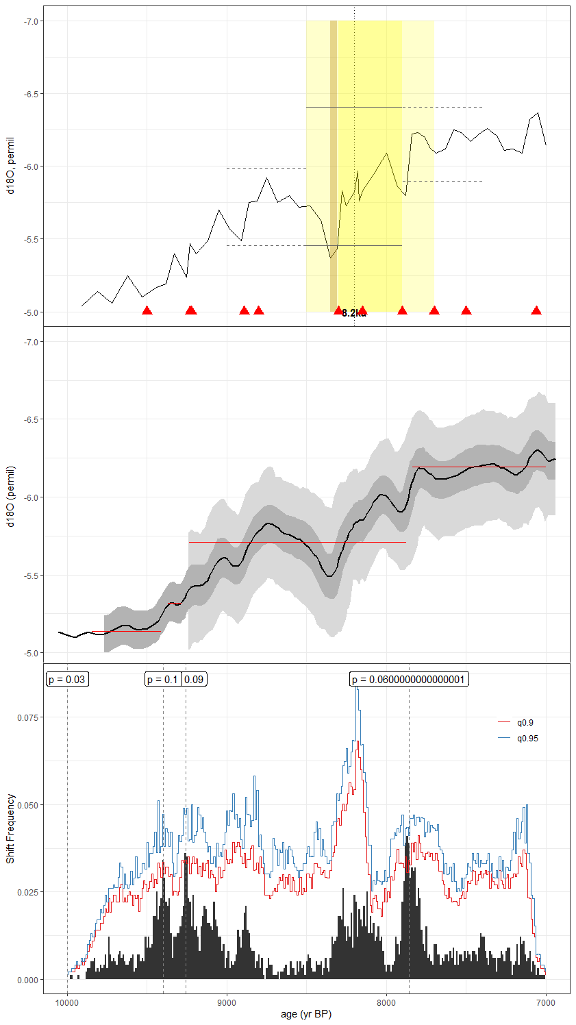
Figure C45 As in Fig. C1, but for the speleothem record of Ayliffe et al. (2013) (LR06_B3_2013). The published age model was constructed by linearly interpolating between radiometric dates. For our analyses, we leveraged the Bchron ensemble published in the SISALv2 dataset.

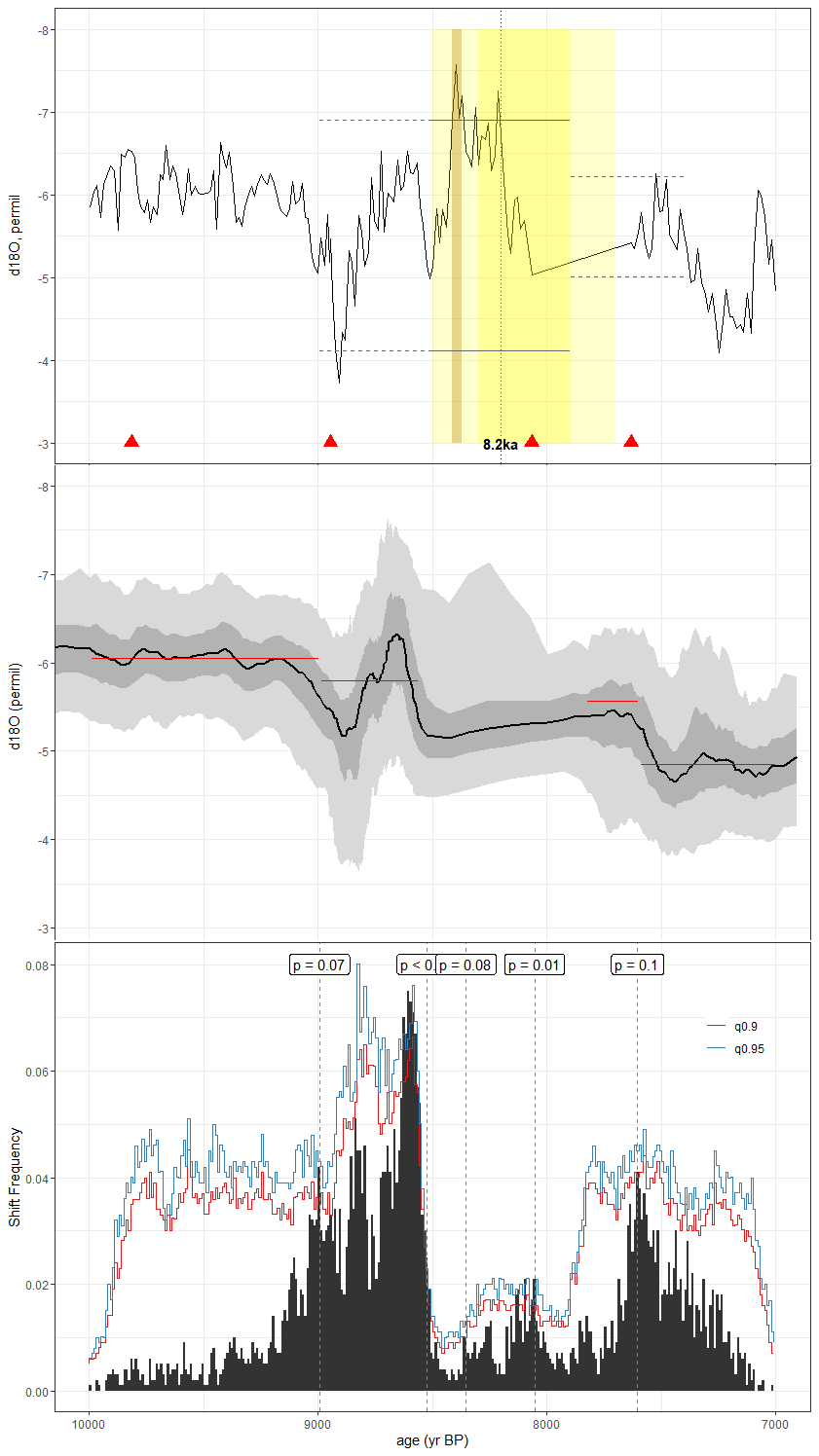
Figure C46 As in Fig. C1, but for the speleothem record of Azevedo et al. (2021) (LSF19). The original method used in the construction of the published age model was unreported, but we use the BACON ensemble supplied in version 2 of the SISAL database for our analyses.

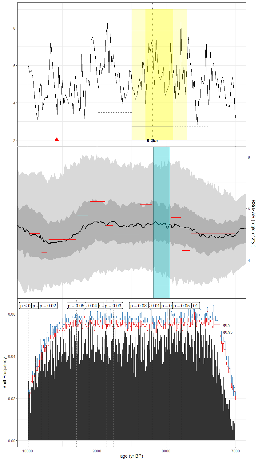
Figure C47 As in Fig. C1, but for the lake sediment BSi MAR record of Johnson et al. (2002) (M981P). CALIB 4.3 was used in the construction of the published age model, with a reservoir age correction of −450 years applied to the radiometric dates. Here, we constructed the age ensemble using the BACON algorithm in geoChronR.

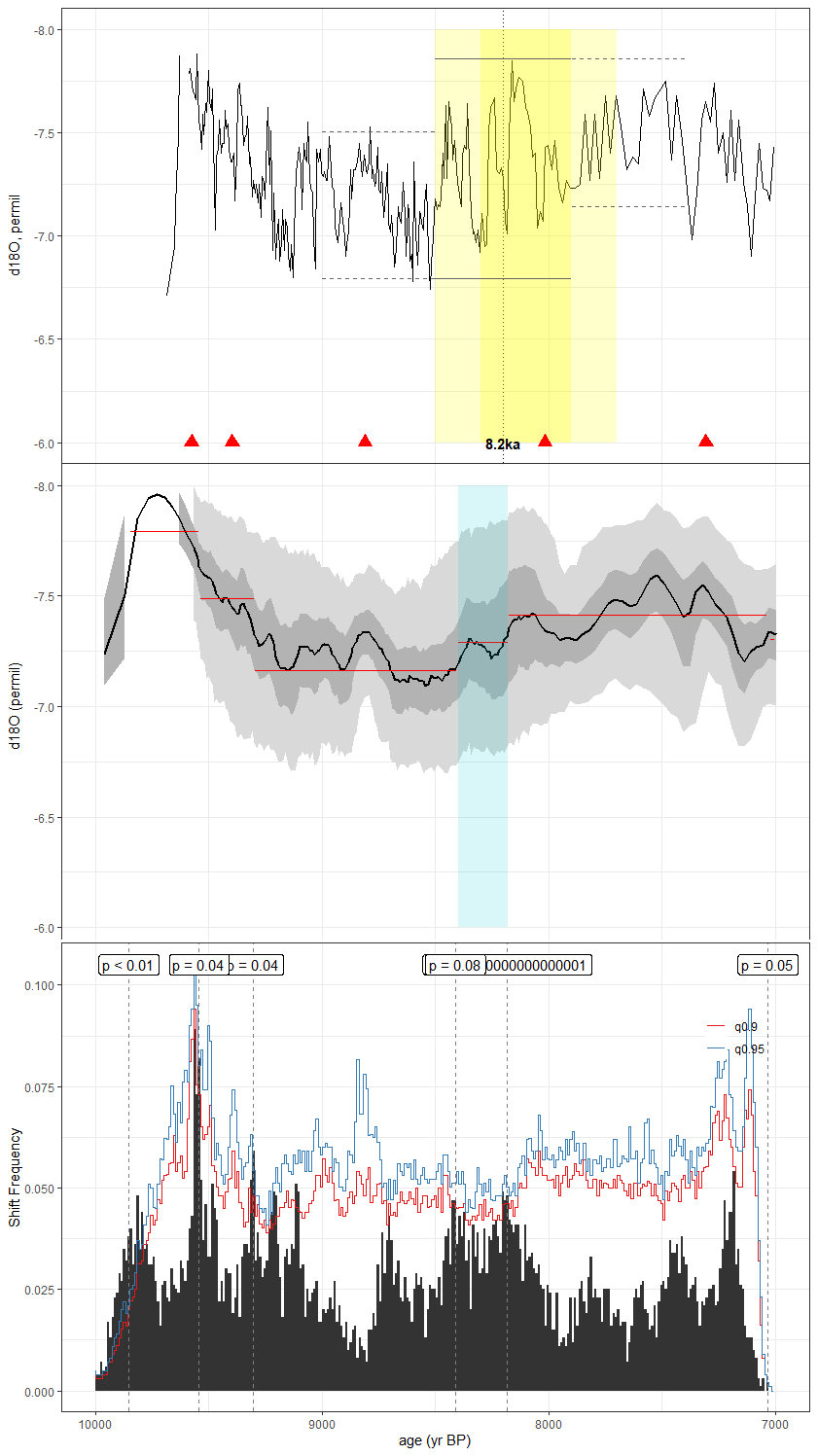
Figure C48 As in Fig. C1, but for the speleothem record of Lechleitner et al. (2017) (MAW6). The published age model was constructed using copRa. Here, we employed the Bchron ensemble included in SISALv2.

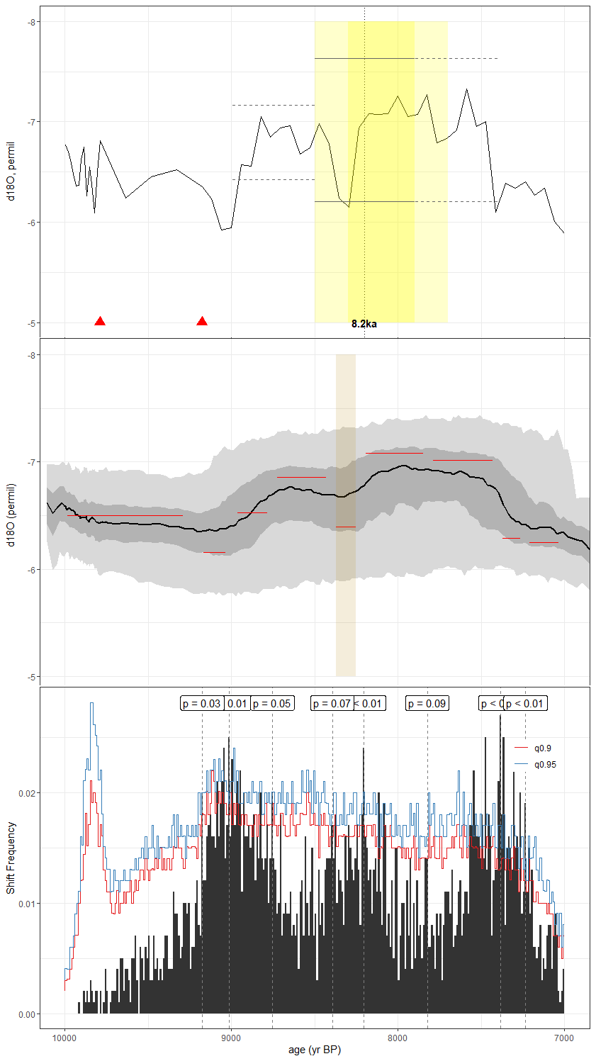
Figure C49 As in Fig. C1, but for the speleothem record of Dutt et al. (2015) (MWS1). The published age model was created using the StalAge algorithm. Here, we use the Bchron ensemble from SISALv2.

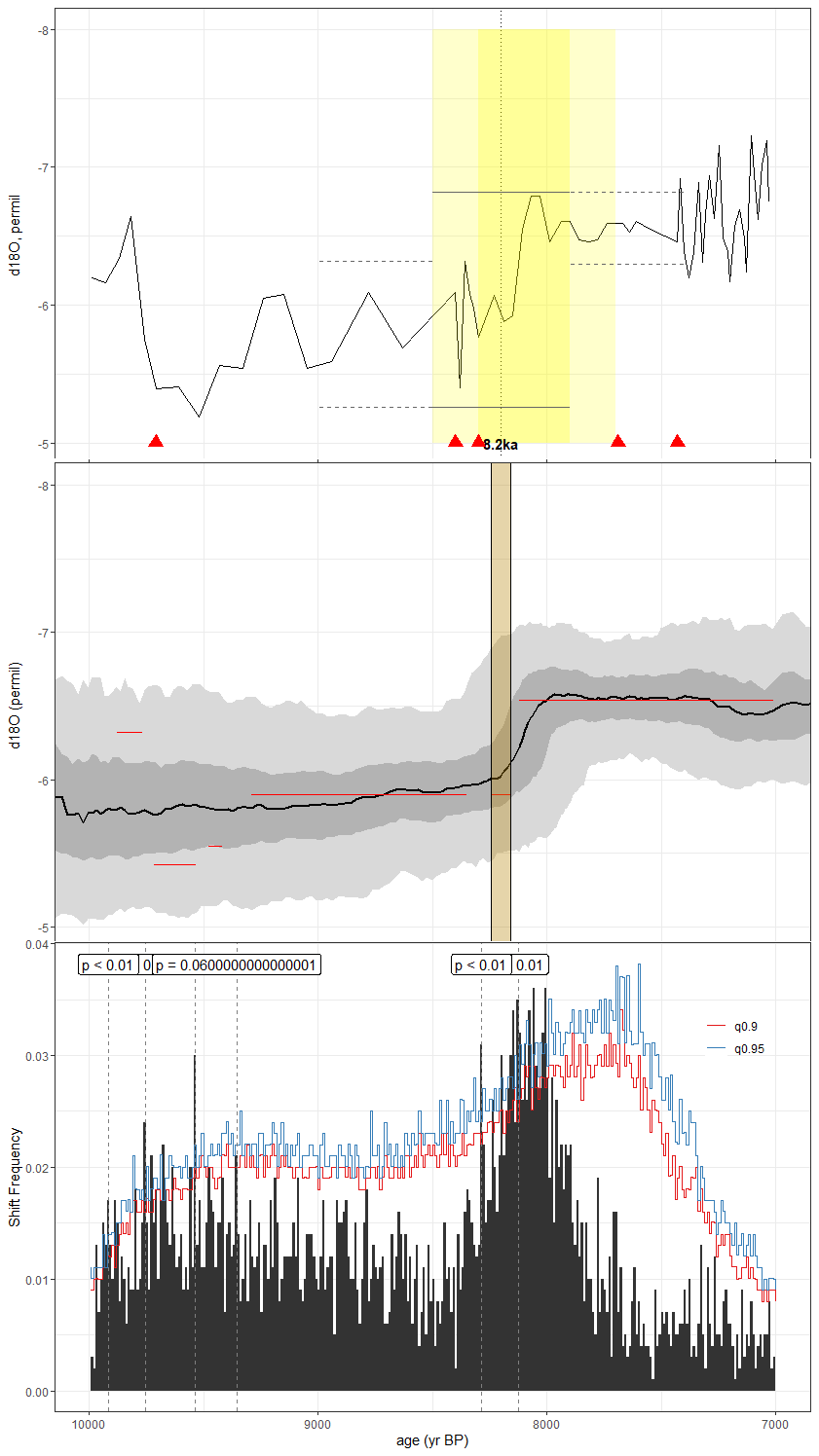
Figure C50 As in Fig. C1, but for the speleothem record of Cheng et al. (2013) (NARC). The published age model was constructed by linearly interpolating between radiometric dates, but here, we leverage the copRa ensemble from the SISALv2 dataset.

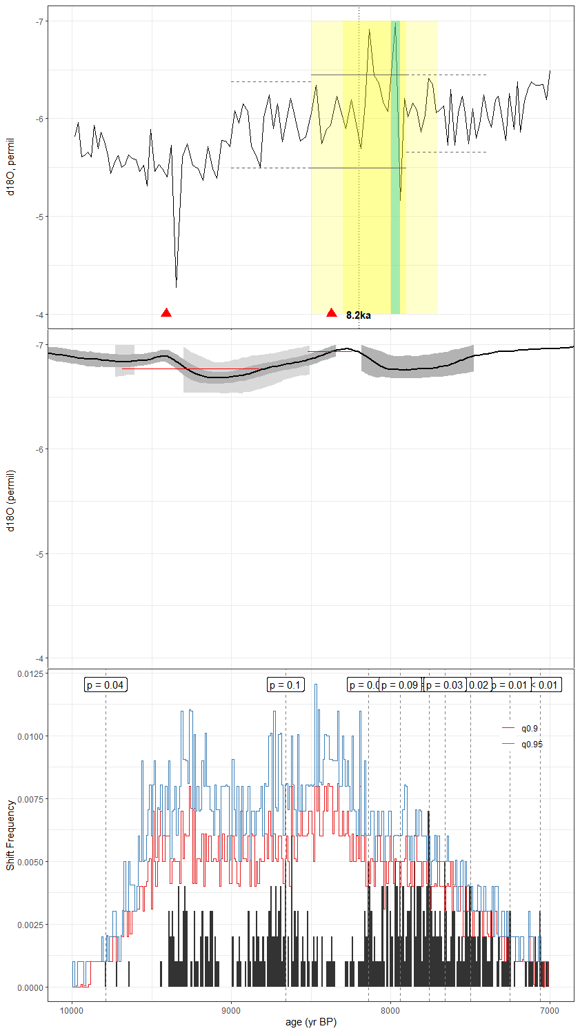
Figure C51 As in Fig. C1, but for the speleothem record of van Breukelen et al. (2008) (NCB). Isoplot 3 was used to construct the published age model, however, we use the SISALv2 BACON age ensemble for our analyses.

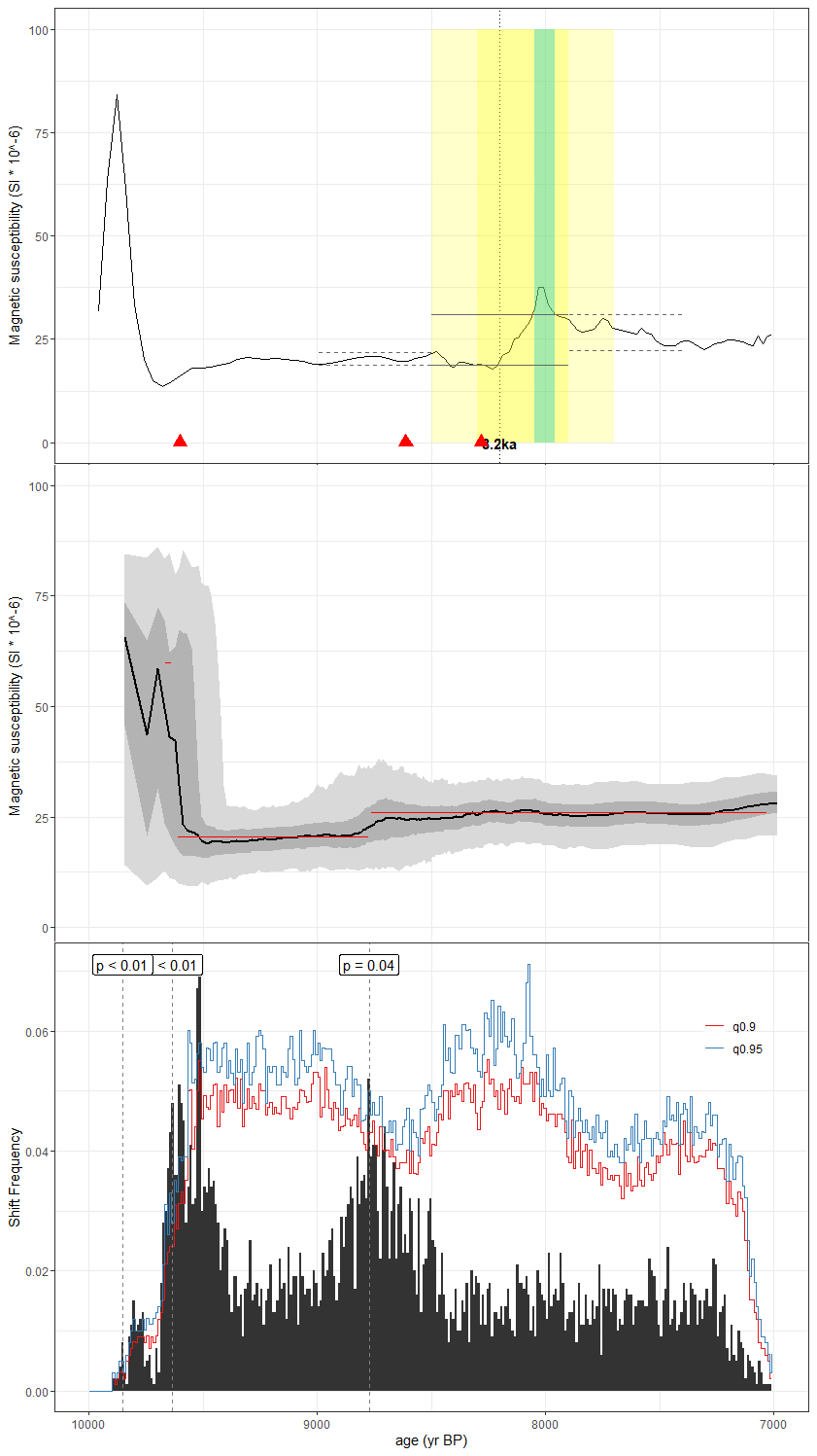
Figure C52 As in Fig. C1, but for the lake sediment magnetic susceptibility record of Escobar et al. (2012) (PET-PI6). The published age model was generated using the OxCal algorithm with IntCal09 calibration curve. Here, we show an age ensemble created using the BACON algorithm with IntCal20 calibration curve generated by geoChronR.

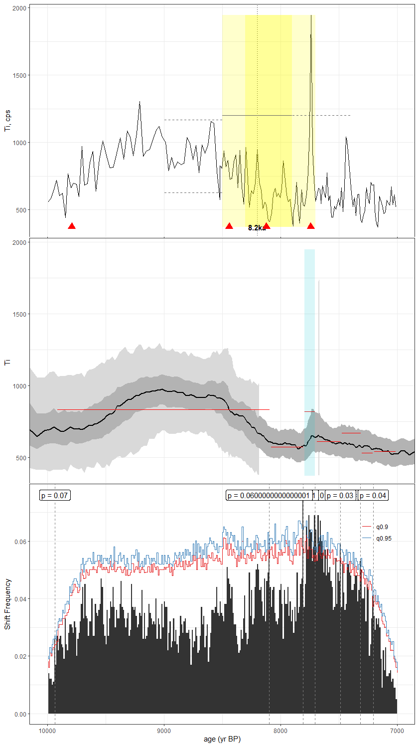
Figure C53 As in Fig. C1, but for the lake sediment titanium content record of Woods et al. (2020) (PLJJUN15). The published age model was created using the BACON algorithm with IntCal13 calibration curve. Here, we reconstruct a BACON ensemble using the IntCal20 curve in geoChronR.

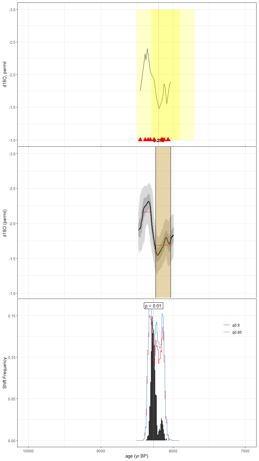
Figure C54 As in Fig. C1, but for the speleothem record of Cheng et al. (2009) (Q5Cheng). The method used in the construction of the published age model is unreported; here, we use BACON in geoChronR to generate our age ensemble.

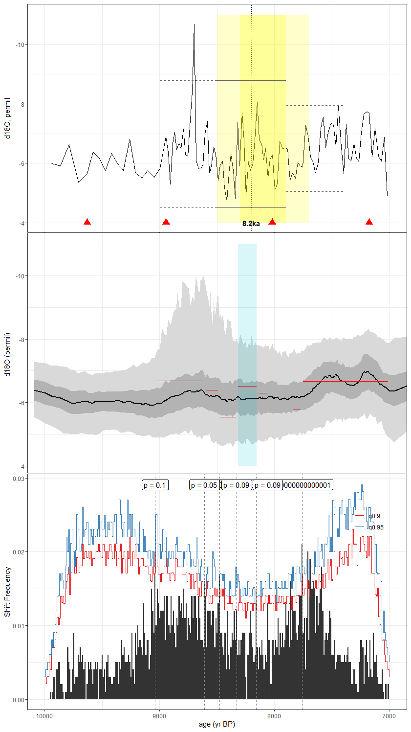
Figure C55 As in Fig. C1, but for the speleothem record of Cruz et al. (2009) (RN4). The method used in the construction of the published age model was unreported, but we leverage the Bchron ensemble supplied in version 2 of the SISAL database for our analyses.

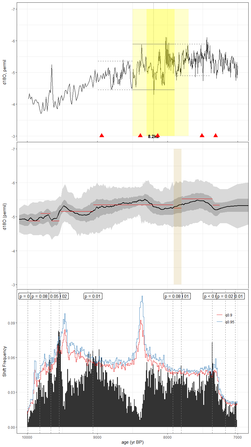
Figure C56 As in Fig. C1, but for the speleothem record of Bustamante et al. (2016) (Sha3). The published age model was developed using copRa. Here, we present the Bchron age ensemble generated for SISALv2.

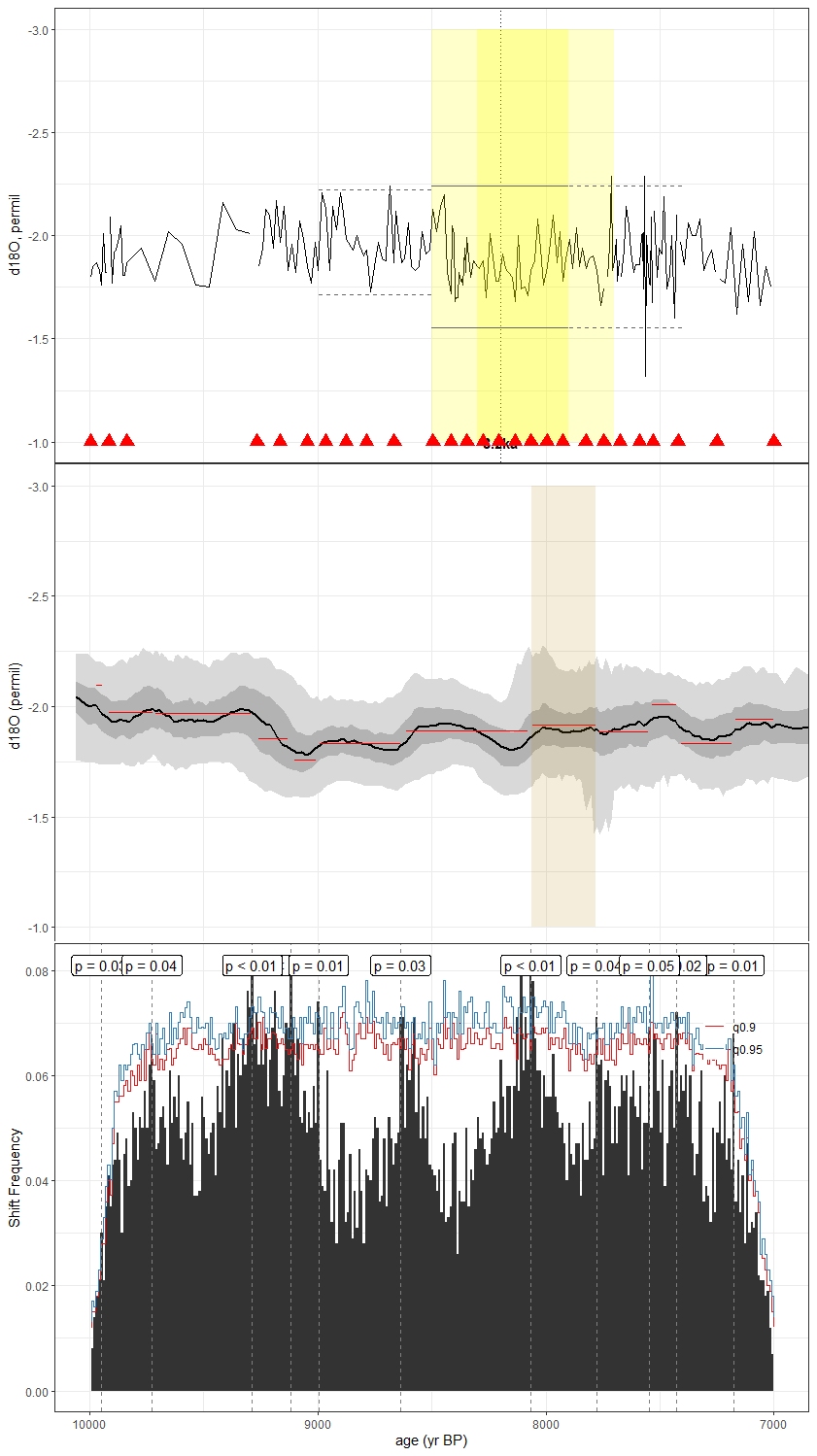
Figure C57 As in Fig. C1, but for the foraminifera record of Staubwasser et al. (2003) (Staubwasser63KA). The published age model was generated via a least-squares regression between ¹⁴C dates using the IntCal98 calibration curve. Here, we constructed our age ensemble using the BACON algorithm and IntCal20 calibration curve in geoChronR.

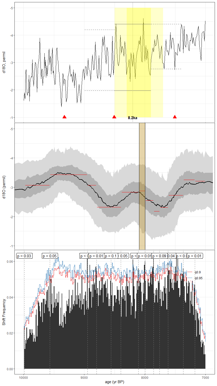
Figure C58 As in Fig. C1, but for the speleothem record of Holmgren et al. (2003) (T8). The published age model was constructed via linear interpolation between dates. Here, we construct our ensemble using the BACON age model algorithm in geoChronR.

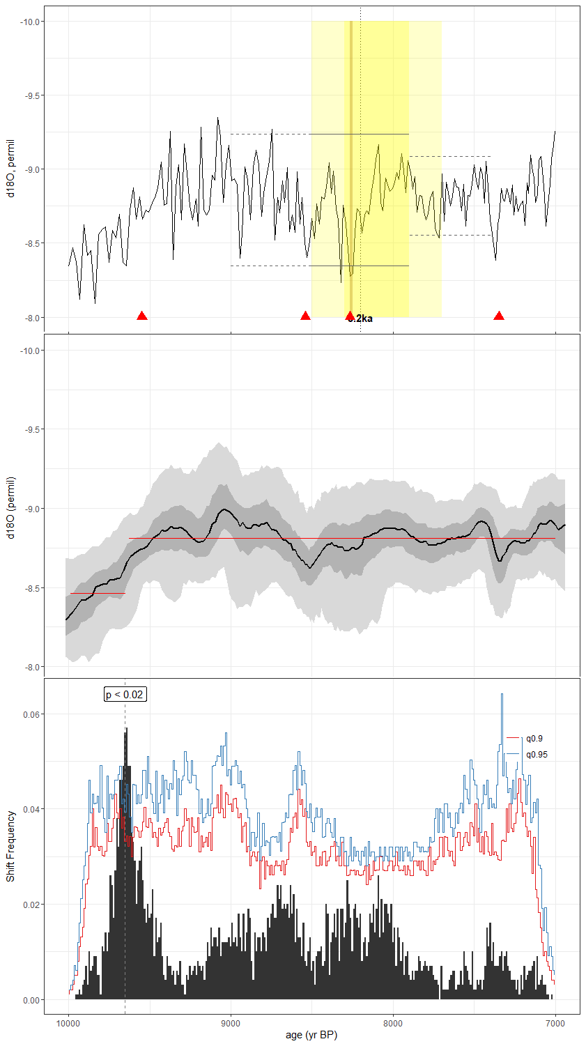
Figure C59 As in Fig. C1, but for the speleothem record of Wurtzel et al. (2018) (TA122). The published age model was constructed using the BACON algorithm. Here, we used the copRa ensemble generated for SISALv2.

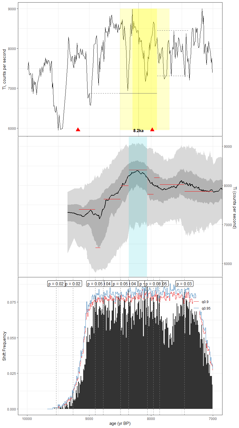
Figure C60 As in Fig. C1, but for the lacustrine sediment record of Russell et al. (2014) (TOW109B). CALIB 6.0 was used to construct the published age model, though we leveraged the BACON algorithm included in geoChronR to generate our age ensemble.

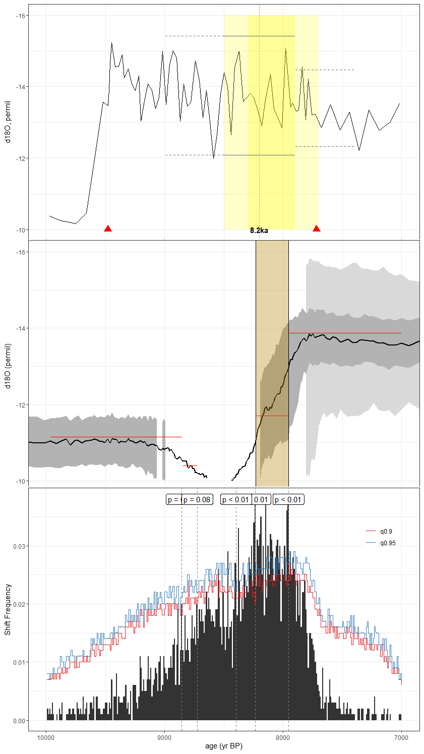
Figure C61 As in Fig. C1, but for the speleothem record of Cai et al. (2015) (XBL29). The published age model was derived from linear interpolation between radiometric dates. For our analyses, we leveraged the SISALv2 Bchron age ensemble.