Deglaciation and abrupt events in a coupled comprehensive atmosphere–ocean–ice-sheet–solid-earth model

During the last 20 000 years the climate of the earth has changed from a state much colder than today, with large ice sheets over North America and northwest Eurasia, to its present state. The fully interactive simulation of this transition represents a hitherto unsolved challenge for state-of-the-art climate models. We use a novel coupled comprehensive atmosphere–ocean–vegetation–ice-sheet–solid-earth model to simulate the transient climate evolution from the Last Glacial Maximum to pre-industrial times. The model considers dynamical changes in the glacier mask, land–sea mask, and river routing. An ensemble of transient model simulations successfully captures the main features of the last deglaciation, as depicted by proxy estimates. In addition, our model simulates a series of abrupt climate changes, which can be attributed to different drivers. Sudden weakenings of the Atlantic meridional overturning circulation during the glacial period and the first half of the deglaciation are caused by Heinrich-event like ice-sheet surges, which are part of the model generated internal variability. We show that the timing of these surges depends on the initial state and the model parameters. Abrupt events during the second half of the deglaciation are caused by a long-term shift in the sign of the Arctic freshwater budget, changes in river routing, and/or the opening of ocean passages.

1 Introduction

The last deglaciation is marked as the transition from the cold climate of the Last Glacial Maximum (LGM; about 21 kiloyears before the year 1950 CE, hereafter referred to as ka) to the modern climate. Driven by gradual changes in the orbital parameters and increasing atmospheric CO₂ concentrations, the climate warmed by several kelvin, and the massive ice sheets over North America and north Eurasia vanished, leading to a strong rise in sea level. Reconstructions of the global mean sea level show a monotonic rise, although with strong temporal variations in the rates of sea-level change (e.g. Fairbanks, 1989; Lambeck et al., 2014). During the main phase of the deglaciation, from 16.5 to 8 ka, the average rate of 12 m ka⁻¹, corresponding to approx. 0.14 Sv (1 Sv =10⁶ m³ s⁻¹) net meltwater input (Lambeck et al., 2014; Hemming, 2004), varied between periods with greater values, e.g. during meltwater pulse 1A (MWP1A, about 14.7 to 13.5 ka; e.g. Carlson et al., 2007; Steffensen et al., 2008; Deschamps et al., 2012; Buizert et al., 2014) with meltwater input rates close to 0.5 Sv (Fairbanks, 1989; Deschamps et al., 2012), and smaller values, e.g. during the Younger Dryas (YD, about 12.8 to 11.7 ka, e.g. Buizert et al., 2014). During the glacial period and the early deglaciation, several abrupt cooling events can be detected in sediment cores from the North Atlantic, containing prominent layers of ice-rafted debris, which originate from melted icebergs that were released from the Laurentide ice sheet into the North Atlantic (Heinrich, 1988). Any addition of large amounts of freshwater into the North Atlantic, whether through melting of icebergs or the direct release of meltwater from the ice sheets themselves, affects the surface salinity, reduces the deepwater formation, and weakens the Atlantic meridional overturning circulation (AMOC). As a result, the northward heat transport reduces and lowers the release of ocean heat into the atmosphere, causing large-scale climate changes. Examples of abrupt events are the cold Heinrich Stadial 1 (H1; about 16.8 ka; Hemming, 2004); the YD; or the rapid Bølling–Allerød (BA) warming, which occurred in between H1 and the YD (about 14.7 to 14.2 ka; e.g. Severinghaus and Brook, 1999; Clark et al., 2002; Weaver et al., 2003; Steffensen et al., 2008).

Various proxy data from marine sediment cores have been used to assess the AMOC state for the glacial climate (Howe et al., 2016) and its variability (Clark et al., 2002; McManus et al., 2004; Lynch-Stieglitz et al., 2014). These data indicate the existence of abrupt climate events, which shaped the sediment record, but even a qualitative estimate of changes in the characteristics of the AMOC remains challenging. For example, even the sign of the AMOC variations is still unclear (e.g. Pöppelmeier et al., 2023). The common consensus, based on studies of the stable δ¹³C isotope or neodymium, is that the position of the AMOC core was shallower during the LGM compared to modern day, but from the current set of available proxy data, it is unclear if and how much the AMOC strength may have changed in comparison to its modern state (see e.g. review of Liu, 2023). From an ensemble of simulations with an Earth System Model of Intermediate Complexity (EMIC) with different AMOC strengths and four proxy tracers, Pöppelmeier et al. (2023) concluded that the global proxy distributions can only be reconciled with an ocean state characterized by a relatively weak AMOC showing a reduction in the circulation strength by 36±8 % (6.3±1.4 Sv) relative to that of the pre-industrial state (PI). However, the sources of uncertainty in this methodology are numerous and diverse. They include an incomplete understanding of the recording and storing of climate signals through proxy data (Dolman and Laepple, 2018; Liu, 2023), as well as a methodological weakness in the reconstruction of the water mass mixing based on proxy data (e.g.  Howe et al., 2016; Oppo et al., 2018; Zhao et al., 2019; Pöppelmeier et al., 2023).

Despite the evidence of abrupt events during the deglaciation from proxies, the causes of the abrupt warming and cooling events and their link to AMOC variations remain uncertain. Understanding the AMOC variability and its drivers therefore requires modelling approaches that span the entire deglaciation. Early modelling studies focused on exploring hypotheses around abrupt events with idealized sensitivity experiments, such as the effect of meltwater release from the ice sheets on the stability of the AMOC (Maier-Reimer and Mikolajewicz, 1989; Schiller et al., 1997; Stouffer et al., 2006; Smith and Gregory, 2009). More recently, the performance of comprehensive coupled climate and earth system models containing both atmospheric and oceanic general circulation model components, as have been used in the Coupled Model Intercomparison Project (CMIP), and their sensitivities to climate perturbations have been evaluated in time-slice experiments of, for example, the LGM or PI (e.g. Harrison et al., 2015; Kageyama et al., 2021). Historically, these models have been developed for the simulation of time periods in which changes in the topography and the ice sheets can be neglected. This assumption does not hold for the last deglaciation and, together with computational demands, represents one of the technical challenges that in large part explains the paucity of transient simulations covering the last deglaciation with comprehensive climate models. Furthermore, transient deglaciation simulations have so far relied on prescribed ice sheets from reconstructions (Liu et al., 2009; Obase and Abe-Ouchi, 2019; He et al., 2021; Kapsch et al., 2022; Bouttes et al., 2023; Obase et al., 2023). Several studies have highlighted that the transient climate response in such simulations, particularly around abrupt events, is dominated by the choice of ice-sheet reconstruction and their type of meltwater forcing (Kapsch et al., 2022; Bouttes et al., 2023; Snoll et al., 2024). A primary example is the meltwater release associated with MWP1A. The main ice-sheet reconstructions utilized in the Paleo-climate Modelling Intercomparison Project Phase 4 (PMIP4; Tarasov et al., 2012; Peltier et al., 2015; Ivanovic et al., 2016) suggest strong meltwater forcing in excess of 0.4 Sv in the Northern Hemisphere for MWP1A. The meltwater release of MWP1A into the North Atlantic results in an AMOC weakening and cold surface temperatures in the Northern Hemisphere. This is not consistent with the subsequent BA warm period as recorded in the Greenland temperature records (Kapsch et al., 2022). This discrepancy between the prescribed meltwater forcing from ice-sheet reconstruction and the ensuing climate response advocates for the inclusion of interactive ice sheets into climate models. However, because of the long characteristic timescales involved in the modelling of ice sheets, they have been mainly included in EMICs (Charbit et al., 2005; Roche et al., 2014; Heinemann et al., 2014; Ganopolski and Brovkin, 2017). The reduced physics, which EMICs are based on, permit the longer integration times necessary for these simulations. Coupling of interactive ice sheets into more computationally expensive comprehensive climate models has so far focused mainly on shorter timescales up to 2 millennia (e.g. Ridley et al., 2005; Mikolajewicz et al., 2007a, b; Vizcaíno et al., 2008; Ziemen et al., 2014; Vizcaíno et al., 2015; Muntjewerf et al., 2020). However, previous modelling efforts often included only a subset of the ice sheets (Charbit et al., 2005; Muntjewerf et al., 2020; Quiquet et al., 2021). In addition, these type of studies typically employed coupling routines, in which the more computationally expensive climate model was accelerated (Charbit et al., 2005; Heinemann et al., 2014; Ziemen et al., 2019), and did not explicitly account for iceberg and solid-earth interactions.

Here we present results from a novel model system that consists of a coarse-resolution version of a comprehensive climate model, includes interactive ice sheets for both hemispheres as well as iceberg and solid-earth interactions, and is applied to the last deglaciation. The model system is described in Sect. 2, and its performance is evaluated for the LGM and PI time slices (Sect. 3.1). We then present an ensemble of transient simulations of the last deglaciation with the new model system (Sect. 3.2) before we focus on the consequences and control of abrupt AMOC-related climate events that are triggered by ice-sheet and topography changes and the associated climate response (Sect.  4.1 and 4.2). The main findings are summarized in Sect. 5.

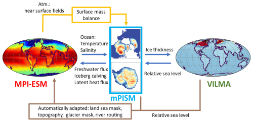
Figure 1 Schematic of the model framework MPI-ESM/mPISM/VILMA with its individual components MPI-ESM, mPISM, and VILMA and the information exchange between the components. As an example, one characteristic property is shown for each model component: surface temperature for MPI-ESM, ice-sheet thickness for mPISM, and relative sea-level change for VILMA.

2 Model and experiment description

2.1 Model

For our study, we use a coupled atmosphere–ocean–vegetation–ice-sheet–solid-earth model. A schematic of the coupled model system is shown in Fig. 1. We provide here only a very brief description of the individual components to focus on the scientific applications.

The climate model is the coarse-resolution version of the Max Planck Institute for Meteorology Earth System Model (MPI-ESM) version 1.2 (Mikolajewicz et al., 2018; Mauritsen et al., 2019) that also has been used for the deglacial simulation described in Kapsch et al. (2022). The atmospheric component is ECHAM6.3 (Stevens et al., 2013). It has a spectral resolution of T31 (corresponding to approx. 3.75° on a Gaussian grid) and 31 levels in the vertical on hybrid coordinates. Land surface processes and vegetation dynamics on land are treated by the JSBACH component (Reick et al., 2013). A hydrological discharge model (Hagemann and Dümenil, 1998) transports the runoff from land to the ocean.

The ocean component is MPIOM1.6 (Jungclaus et al., 2013). It has a resolution of 3° on an Arakawa C grid (Arakawa and Lamb, 1977) with the grid poles located in southeast Greenland and in the centre of Antarctica, yielding a relative high resolution in the North Atlantic subpolar gyre (35 to 150 km). The ocean model has 40 levels on z coordinates, with layer thickness increasing towards depth, a free surface, and a mass flux boundary condition. Vertical mixing and diffusion are based on a Richardson-number-dependent formulation by Pacanowski and Philander (1981). In addition, a simple mixed-layer scheme describes near-surface mixing. For the background mixing, a fixed vertical profile is assumed. Starting with a given surface value, it increases linearly with depth until 1000 m. Below it is constant. A sea-ice component with viscous plastic rheology following Hibler (1979) with 0-layer thermodynamics including snow is embedded in MPIOM. In addition, the version of MPIOM used here contains a new dynamic/thermodynamic Eulerian iceberg model with five size classes (Erokhina and Mikolajewicz, 2024), allowing the explicit treatment of calved icebergs, their subsequent drift, and a three-dimensional input of meltwater and latent heat release.

For the assessment of the past circulation changes, proxy data are the only source of information. Therefore, we included an artificial water mass tracer (dye) in the ocean component to gain a better insight into how circulation changes would be reflected in proxy data. The dye indicates the relative contribution of water originating from the surface of the North Atlantic and the Arctic and thus is tracing the relative contribution of North Atlantic Deep Water (NADW) at depth. The boundary condition of the dye at the surface is 1 in the source area (see Fig. A2) and 0 outside this area. In the ocean interior, the dye is advected and mixed like salinity.

Ice sheets are represented by the thermomechanically coupled ice-sheet model mPISM (Ziemen et al., 2019) based on PISM0.7.3. The ice dynamics in mPISM are based on the superposition of the shallow-ice and shallow-shelf approximations, making it suitable to model slow ice flow, fast ice flow, and grounding-line migration. The polar stereographic grid has a resolution of 10 km in the Northern Hemisphere and 15 km for Antarctica. The surface mass balance (SMB) of the ice sheet is calculated by an energy balance model using hourly atmospheric input data from the atmospheric model component ECHAM6.3 (Kapsch et al., 2021) on 24 different height levels on the atmospheric grid. This three-dimensional SMB field is then interpolated onto the actual surface topography of the ice-sheet model.

The response of the solid earth and changes in relative sea level, induced by the consistent redistribution of ice and water masses, are computed with the global VIscoelastic Lithosphere and MAntle model (VILMA, Martinec et al., 2018). VILMA is employed in its 1D configuration, which assumes that the viscosity structure of the earth varies only with depth. VILMA solves the sea-level equation, accounts for rotational feedback, and considers an incompressible self-gravitating viscoelastic material with a Maxwell rheology. The sea-level equation is solved on the horizontally discretized Gaussian F128 grid (approx. 0.7°), which represents the resolution at which data are exchanged, i.e. the ice-sheet distribution as input and the negative relative sea-level change, representing the change in topography due to glacial isostatic adjustment (e.g. Konrad et al., 2015).

The coupling time step between the atmosphere and ocean model is 1 d. The iceberg model is part of the ocean model and thus interacts at every ocean time step. The MPI-ESM is coupled every 10 years with the ice-sheet and solid-earth models. At this interval, new high-resolution topographies ($\mathrm{1}/\mathrm{6}\mathit{°}$ horizontal resolution) are calculated from the results of VILMA and mPISM and used to derive adapted topographies (including land/sea masks) for the ocean and the atmosphere using the algorithm developed by Meccia and Mikolajewicz (2018). River-routing directions are adapted dynamically according to topography changes using the algorithm developed by Riddick et al. (2018). The ice-sheet model supplies calving fluxes to the iceberg module. A reduced version of this model system without the iceberg module, interactive ice sheets, and solid-earth dynamics has been used by Kapsch et al. (2022) to perform deglacial simulations using prescribed ice-sheet reconstructions. We refer to the model framework in the following as MPI-ESM/mPISM/VILMA.

2.2 Experiments

For all simulations, the atmospheric concentrations of CO₂, CH₄, and N₂O were prescribed according to Köhler et al. (2017). Earth orbital parameters were calculated following Berger and Loutre (1991). In addition, in most simulations, annually varying volcanic forcing (Schindlbeck-Belo et al., 2024) was prescribed for the time after 26 ka.

To achieve a physically consistent initial state for 26 ka, transient asynchronous spin-up simulations were started from one existing glacial state of the model system. These asynchronous simulations cover the period from 45 to 26 ka. During the asynchronous spin-up, MPI-ESM was run for 10 years, providing the forcing for a 100-year simulation with mPISM and VILMA. Subsequently, freshwater and iceberg supply from the ice sheets and topography and bathymetry changes from mPISM and VILMA are considered in the next 10-year simulation with MPI-ESM. This procedure was repeated over the entire asynchronous spin-up period from 45 to 26 ka, yielding a spin-up of 19 000 years for mPISM and VILMA and 1900 years for MPI-ESM. This acceleration of a factor of 10 saves considerable amounts of computing time and serves to spin up the model components with the longest memory. A climatological volcanic forcing was used in the spin-up integrations to avoid large artificial variability.

A set of eight synchronously coupled transient deglacial experiments with different model parameter settings were started from asynchronous spin-up simulations at 26 ka. For an overview of the ensemble members see Table 1.

We do not consider the first 1000 years of each simulation for our analysis to circumvent the effects of minor adjustments after the switch to the synchronously coupled simulation. Thus, our analysis covers only the time from 25 ka to 1850 CE. For the LGM time slice, the simulations had a spin-up for atmosphere and ocean without parameter changes for 4900 years (3000 years for D1.2 and D1.3), ensuring sufficient adjustment time to the transient forcing.

Effectively, our full ensemble consists of two smaller separate sub-ensembles, each containing four members. The first sub-ensemble explores the effect of vertical mixing in the ocean. Schmittner et al. (2015) used a combination of a tidal model and an EMIC to investigate the effect of enhanced tides during the glacial and report a change in global mean diapycnal mixing of more than a factor of 3 compared to PI. Since the background mixing is rather poorly constrained and includes in our mixing scheme a variety of processes, e.g. tidal mixing, we investigate the sensitivity to this parameter in the first sub-ensemble. Here, D1.1 serves as the baseline experiment. All four members of this sub-ensemble start from the same asynchronous spin-up simulation. In experiment D1.2 the vertical background mixing coefficient was increased, while in experiment D1.3 it was decreased. All experiments of this sub-ensemble used a climatological volcanic forcing representing PI, with the exception of D1.4, which was forced with the time-varying volcanic forcing (Schindlbeck-Belo et al., 2024).

For the second sub-ensemble, D2.1 is the baseline experiment. In comparison to D1.1, several parameter values within the individual ESM components were changed. This includes changes in sea-ice parameters towards a more rigid sea ice (like Hunke and Dukowicz, 1997, in comparison to Hibler, 1979) and reduced drag between the ocean and sea ice. The latter is motivated by the fact that the katabatic winds and consequently the sea-ice transports in this model are somewhat underestimated due to the coarse resolution of the atmospheric component. Additionally, the prescribed vertical profile of oceanic background mixing was reduced in the upper ocean. This was motivated by the results of the first ensemble, which show a large effect of the prescribed background mixing on the AMOC (see Sect. 3.1) but also a strong effect on the age distribution of the water masses especially in the Pacific (not shown). To maintain both a reasonable age distribution in the deep ocean for PI as well as a more realistic glacial AMOC, the reduced mixing was restricted to the upper ocean. As the treatment of the ocean surface velocities in the coupling interface of the atmosphere was discovered to be affected by a bug, this part of the coupling was suppressed in all simulations of this sub-ensemble. To maintain a similar climate in terms of the surface temperatures, small changes in the atmospheric parameters were required to reduce a slight cold bias. Changes in the ice-sheet parameters in comparison to the first sub-ensemble focused on enhanced sliding and a more sensitive basal mass balance. The goal behind the enhanced sliding tuning was twofold: first, we targeted a faster expansion of the ice sheets towards the LGM; second, the resulting thinner ice sheets facilitate ice-sheet retreat during the deglaciation. The more sensitive basal mass balance was targeted towards a faster retreat of the marine portions of the Antarctic ice sheets. All runs in this sub-ensemble were run with time-varying volcanic forcing and start from their own matching asynchronous spin-up.

In addition, two sensitivity experiments (D2.1.1 and D2.1.2) were performed to investigate the effect of initial conditions for the ice sheets on the deglacial climate trajectory. Except for the initial conditions they are identical to D2.1. These experiments are analysed in Sect. 4.2 and are not included in our main ensemble. Experiment D2.1.1 was only integrated until 7 ka.

Table 1 Ensemble members with their parameter settings and spin-up procedures. Detailed individual parameter changes are listed in Tables A1 and A2. In all asynchronous spin-up simulations climatological volcanic forcing was used.

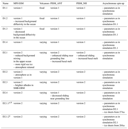
^a The sensitivity studies D2.1.1 and D2.1.2 are not part of the ensemble. ^b D.2.1.1 was run only until 7 ka.

3 The simulated climate

To evaluate the simulated climate, we first show the model results for the time of the LGM. The LGM has been intensively investigated for steady-state time-slice simulations (21 ka), as it is a standard time slice within PMIP4 (e.g. Kageyama et al., 2020). In Sect. 3.2 we will present the simulated transient deglacial climate changes.

3.1 LGM climate relative to PI

Since our model runs show substantial millennial-scale variability throughout the glacial period (see Sect. 4.2), we chose to average the LGM state over the time window from 23 to 18 ka. In the Holocene, millennial-scale variability is rather small; thus only 1000 years (1100 to 100 yr BP) were used for the calculation of the PI climate state. In addition to the ensemble median, minimum, and maximum, we also show results from one particular experiment (D2.1), which we use in Sect. 4.1 to discuss the deglacial climate variability in more detail.

Figure 2 Mean annual surface air-temperature anomalies in kelvin (K) with respect to PI for different regions: (a) the global mean and the mean over (b) the southern extratropics (90–30° S), (c) the tropics (30° S–30° N), and (d) the northern extratropics (30–90° N). Each panel shows values derived from reconstructions (left) (Friedrich et al., 2016; Bereiter et al., 2018; Tierney et al., 2020; Osman et al., 2021; Annan et al., 2022, and the PalMod reconstructions), the PMIP4 model ensemble (centre Kageyama et al., 2020), and our model ensemble (right). Whiskers on the reconstructions indicate uncertainties.

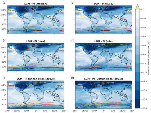
Figure 3 Difference in annual mean near-surface air temperature between LGM and PI in kelvin (K; colours). The panels show (a) the ensemble median, (b) the results for simulation D2.1, (c) the ensemble maximum, and (d) the ensemble minimum. Please note the ensemble minimum/maximum indicates the minimum/maximum value occurring in any of the ensemble members at each grid point. The isolines show sea-ice extent (>0.15 sea-ice coverage in the long-term mean seasonal climatology) for PI summer (solid yellow) and winter (dashed yellow) and LGM summer (solid red) and winter (dashed red). The bottom panel shows reanalysis results from (e) Annan et al. (2022) and (f) Osman et al. (2021). The LGM sea-ice margin plotted in the bottom panels is taken from the GLOMAP (Paul et al., 2021) reconstruction, and the PI reference has been calculated from years 1951 to 1990 from the HadISST data set (Hurrell et al., 2008). PI and LGM land–sea masks are indicated by the solid and dashed black lines, respectively.

3.1.1 Near-surface air temperatures

The simulated global mean LGM near-surface air temperature (SAT) in our model ensemble is 5.0 to 5.8 K colder than the PI reference state (Fig. 2a). The simulated cooling pattern shows a strong polar amplification illustrated by the significantly larger cooling in the high northern latitudes (9.1 to 9.8 K) than in the tropics (between 3.0 and 3.5 K; Fig. 2d and c). In the southern high latitudes, the simulated LGM climate is between 4.6 and 6.3 K (mean: 5.1; median: 4.8) colder (Fig. 2b). These values lie well within the LGM (21 ka) climate signal from the PMIP4 ensemble (3.7 to 6.8 K). Our estimates also agree well with estimates of LGM SAT anomalies from available reanalysis and reconstruction data sets (see Fig. 2). For validation, we use recent products either based entirely on proxy data (such as the PalMod reconstructions, based on the methodology and proxy data described in Baudouin et al., 2025, see Appendix A2) or data assimilation products that use either a single model (Tierney et al., 2020; Osman et al., 2021) or an ensemble of models (Annan et al., 2022). Globally, our simulated SAT anomalies (mean: −5.2 K; median: −5.1 K) align with the range of reconstructed SAT anomalies of the PalMod reconstructions (Appendix A2) of −4.1 and −7.1 K (mean: −5.6 K) and the reanalysis of Friedrich et al. (2016) of −6.5 to −3.5 K (mean: −5.0 K) and Annan et al. (2022) of −2.9 to −6.0 K (mean: 4.5 K). The reanalyses of Osman et al. (2021) and Tierney et al. (2020) and to a smaller extent the reconstructions of Bereiter et al. (2018) are consistently colder than our ensemble (−6.3 to −7.4 K, −5.7 to −6.5 K, and −7.5 to −5.1 K, respectively) and the Annan et al. (2022) data assimilation product. The same signal is present through regional estimates for the northern and southern extratropics and tropics, where our ensemble mean is slightly colder than Annan et al. (2022) but warmer than Osman et al. (2021) and Tierney et al. (2020). Thereby nearly all ensemble members fall into the uncertainty range of the Annan et al. (2022) estimates, except for D1.3 for the tropics and southern extratropics.

Maximum cooling is simulated over the Laurentide and Fennoscandian ice sheets (Fig. 3), where the higher surface elevation leads to an additional cooling effect. Also the North Atlantic shows a rather strong cooling, which is related to extended sea-ice cover (Fig. 3). In general, the simulated pattern of cooling is rather similar to the ensemble mean pattern from the CMIP6 LGM time-slice simulations (Kageyama et al., 2020, their Fig. 1) and the reanalysis product of Annan et al. (2022). The spatial pattern of the reanalysis product by Osman et al. (2021) is also very similar to our ensemble, but the amplitude of the cooling is considerably stronger. The bias of the simulated PI SAT and sea-ice edge compared to an observation-based estimate is shown in Fig. A1.

3.1.2 Sea-ice extent

The simulated sea-ice extent on the Northern Hemisphere for the PI period is fairly close to the extent derived from the HadISST data set for the years 1951 to 1990 (Hurrell et al., 2008; see isolines in Figs. 3 and A1). The main discrepancy is an underestimation of the sea-ice extent in the Southern Ocean.

For the LGM, the ensemble spread for the winter sea-ice extent in the North Atlantic is considerable. Some simulations show an ice-free northeast Atlantic and others a state with winter sea ice that covers nearly the entire North Atlantic north of 40° N. The northwest Atlantic is seasonally sea ice covered in all simulations. In the North Atlantic, the GLOMAP reconstruction (Paul et al., 2021) does not show a large difference between the northwest and northeast Atlantic. It is worth noting that simulation D2.1 does not show such a contrast either. The Norwegian Sea is only seasonally covered by sea ice in all simulations, whereas most of the Greenland Sea and Iceland Sea are permanently covered by sea ice. GLOMAP indicates seasonal sea-ice cover in the entire Nordic Seas, with the LGM summer sea-ice margin even being north of its position in the 20th century in the HadISST data set (Hurrell et al., 2008). The simulated Southern Ocean sea-ice cover is seasonal, except for some regions close to the coast of Antarctica. The model generally underestimates the summer sea-ice extent in the Southern Hemisphere, both for PI as well as for LGM. The simulated winter sea-ice extent in the Southern Ocean matches the GLOMAP data set well.

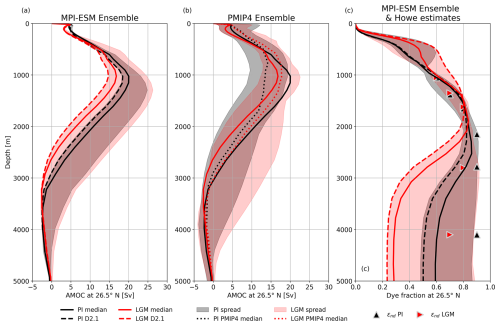
Figure 4 (a) Depth profiles of the simulated AMOC at 26.5° N for the ensemble median (solid lines) and the ensemble spread (shadings) for PI (black) and LGM (red). Dashed lines highlight the results of D2.1. (b) Same as panel (a) but based on the PMIP4 ensemble (Kageyama et al., 2020), with the ensemble median given as dotted line. For better comparison, the ensemble medians from panel (a) are shown as well (solid lines). (c) Depth profiles of the zonally averaged relative contribution of water originating from the surface of the North Atlantic or the Arctic at 26.5° N (dye fraction). Same colour coding as in panel (a). Overlaid are estimates based on neodymium composition ε_Nd from Howe et al. (2016) (black triangles for PI, red triangles for LGM).

3.1.3 AMOC

The maximum strength of the NADW cell at 26.5° N, which defines the AMOC strength, varies in our PI ensemble between 18.3 and 24.8 Sv (ensemble median is 20.0 Sv) and is located at a depth slightly deeper than 1000 m (see profile of the AMOC at 26.5° N in Fig. 4a). From measurements of the RAPID array at the same latitude for the years 2004 to 2017, the strength of the AMOC has been estimated to be 17.0 ± 4.4 Sv (Frajka-Williams et al., 2019; Moat et al., 2023). The strength of the Antarctic Bottom Water (AABW) cell at 26.5° N varies between 0.4 and 2.5 Sv for the PI ensemble.

For the LGM, the spread of the AMOC strength is much larger, showing values between 14.7 and 26.3 Sv, with an ensemble median of 16.8 Sv. Except for simulation D1.2, all runs show a shallower and slightly weaker AMOC cell during the LGM than for their PI counterpart. The vertical extent of the NADW cell, for which the lower boundary is defined as the depth below 2000 m where the AMOC strength equals zero, becomes shallower by 250 to 450 m for almost all individual ensemble members. However, both the spread of the maximum strength of the NADW cell as well as that of the depth of its lower margin are about twice as large for the LGM as compared to the PI simulations. The prescribed vertical background mixing in the ocean has a very large effect on the AMOC profile, as can be seen from comparing simulations D1.2, D1.1, and D1.3 (see Fig. A3a). Lower vertical mixing reduces ocean heat transport to high southern latitudes, which results in a substantial cooling (2.4 K colder LGM SATs south of 60° S in D1.3 compared to D1.1). This enhances sea-ice formation and thus brine release. For the LGM, the integrated brine release in locations with a positive net sea-ice formation in the Southern Ocean is 28 % higher in D1.3 compared to D1.1 (calculated from decadal mean data), resulting in saltier and denser AABW. Glacial NADW becomes colder as well but also fresher. Thus, the effective change in density is much smaller than in the south, similar to the findings of Klockmann et al. (2016). The reduced vertical mixing enables a prolonged preservation of the density excess of AABW compared to NADW on its path towards the deep North Atlantic. The consequence is a weakening and shallowing of the NADW cell and an enhanced presence of AABW (see Fig. A3b). Stronger vertical mixing has the opposite effect and leads to a LGM AMOC that is even stronger and deeper than its PI counterpart. Overall, the effect of changes in vertical mixing on the AMOC is larger for the LGM than for PI.

Wunsch (2003) has suggested that the reduced shelf area during LGM leads to stronger tides. Wilmes et al. (2019) applied a tidal model and report an enhanced energy supply from tides to the internal wave field (1.8 to 3 times higher for LGM than at present, depending on the ice-sheet geometries). As we used a time-constant background mixing in our simulations, this effect is not included.

For the PMIP4 ensemble, most LGM simulations show a weak deepening and a substantial strengthening of the AMOC (Fig. 4b). This is in contrast to estimates based on proxy data that indicate a shallowing of the AMOC core and a reduction of the circulation strength (e.g. Pöppelmeier et al., 2023), in line with our results.

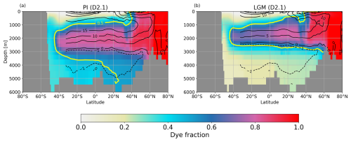
Figure 5 Atlantic section of the zonal mean dye fraction for (a) PI and (b) LGM for one ensemble member (D2.1). Overlaid are contour lines of the AMOC strength (black lines at −1, 0, 5, 10, and 15 Sv) and one contour line of the dye fraction (yellow line =0.5 as an indicator of the boundary between NADW and AABW).

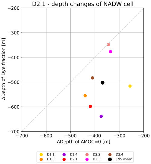
Figure 6 Depth changes between LGM and PI of the dye fraction for the concentration being found for AMOC =0 in PI versus that of AMOC =0 at 26.5° N. Ensemble members and ensemble mean are shown (see legend). D1.2 has been excluded from this analysis (see text). The dashed light-grey line indicates the 1:1 depth change for orientation.

For the assessment of the past AMOC changes, we analyse changes in the dye tracer, which indicates the relative contribution of the water masses originating from the surface of the North Atlantic and Arctic. A decreasing dye fraction reflects the larger contribution of water which originates from other source regions, which in the Atlantic below 2000 m is primarily AABW. The dye fraction at 26.5° N shows the core of NADW for PI at depths between 1500 and 3000 m (Fig. 4c). The depth of 3000 m corresponds to the lower margin of the AMOC cell. Below 3500 m, the intrusion of AABW becomes visible as a thick layer of water that consists of a mix of NADW and AABW. For the LGM, the core of the NADW lies shallower and has a reduced vertical extent. The deep layers are dominated by AABW. Estimated changes in the NADW distribution from proxy data show a qualitatively similar pattern (Howe et al., 2016; Oppo et al., 2018; Gu et al., 2020). Note that the reconstruction of the data by Howe et al. (2016) is based on neodymium isotopes, which might underestimate changes in NADW at the LGM due to their source being at the continental slope (Liu, 2023), unlike other proxies and our dye tracer, which have their source solely at the surface. Reduced vertical mixing leads to stronger differences in the dye profile at 26.5° N between LGM and PI (see Fig. A3b) in line with the AMOC changes.

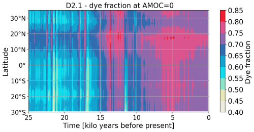
Figure 5 illustrates the distribution of the dye fraction and the location and strength of the cells of NADW and AABW at the PI and the LGM for one ensemble member (D2.1). In agreement with the shallowing of the lower boundary of the NADW cell at the LGM, the vertical extension of the dye fraction higher than 0.5 is limited to the upper 2500–3000 m. Qualitatively, the shift of the distribution of water masses between PI and LGM in our ensemble follows the changes derived from proxy data (Howe et al., 2016; Menviel et al., 2017; Oppo et al., 2018; Gu et al., 2020). However, quantitatively, the change in the AMOC geometry is different from the change in the spatial pattern of the dye fraction. If the lower boundary of the NADW cell is confined by AMOC =0, a dye fraction of about 0.5 is found at a very similar depth at the LGM. For the PI, the dye fraction at AMOC =0 is much higher (around 0.7), and NADW is the dominant water mass in the deep Atlantic north of 20° N. Our dye fraction provides the opportunity to compare simulated depth shifts of the lower boundary of the AMOC cell to changes in the location of NADW identified by the dye fraction (Fig. 6). As already apparent from D2.1 in Fig. 5, almost all ensemble members show that the shallowing of the dye fraction for the LGM is more pronounced than the shallowing of the NADW cell. Ensemble member D1.2, in which the AABW cell does not extend to 26.5° N, has been excluded from this analysis. For the ensemble mean, the depth change in the water mass boundary indicated by the dye fraction is about 35 % larger than that for the AMOC cell boundary. Note that the dye fraction has no methodological uncertainty and no potential variations in the source function as is the case for proxy data (Howe et al., 2016; Gu et al., 2020; Liu, 2023). The simulated temporal and spatial variations of the dye fraction at AMOC =0 are a result of water mass mixing intensity and emphasize how complicated a straightforward assessment of the AMOC geometry is based on proxy data (see a further discussion in Appendix A5 and Fig. A4). The simulated difference therefore provides a cautionary note for a quantitative validation of AMOC changes with proxy-derived changes in water mass boundaries.

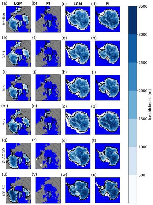
Figure 7 Ice thickness maps for the Northern Hemisphere and Antarctica. The column title indicates the respective time slice. The rows correspond to (a–d) the ensemble median, (e–h) D2.1, (i–l) the ensemble minimum, (m–p) the ensemble maximum, (q–t) ICE-6G, and (u–x) GLAC-1D. The thick black line indicates the median position of the grounding line. Ice volumes for ice sheets for the LGM and PI are provided in Table A3.

3.1.4 Ice sheets

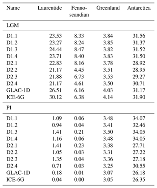
The simulated Laurentide ice sheet for the LGM has a similar size as in the GLAC-1D reconstructions (Tarasov et al., 2012; Briggs et al., 2014) and ICE-6G (Peltier et al., 2015), as shown in Fig. 7. Similar to other studies (Ziemen et al., 2014; Sherriff-Tadano et al., 2024), the largest differences occur at the southeastern margin, where the reconstructions extend further south than the Laurentide ice sheet in the simulations. Moreover, the simulated Laurentide ice sheet shows a clear two-dome structure – one dome covering the Cordilleran (western Laurentide) ice sheet and the second, more prominent dome, covering the eastern Laurentide. The latter is not distinctly visible in the reconstructions. However, the reconstructions exhibit considerable uncertainties, especially in the thickness distribution. Differences in ice thickness between the modelled Laurentide ice sheet and reconstructions are most prominent in the Hudson Bay and Mackenzie areas. Both regions frequently exhibit Heinrich event (HE)-like surge events (e.g. Heinrich, 1988; Ziemen et al., 2019; Schannwell et al., 2023) in our model, which will be discussed in more detail in Sect. 4.1. The impression that the Labrador Sea is covered by an ice shelf in our simulations stems from the fact that we average over periods with HE-like surge events, during which a temporary ice shelf forms (Fig. 7a, e, and m), and more frequent periods without an ice shelf in the central Labrador Sea. The model simulates a Fennoscandian ice sheet that is in good agreement with the reconstructions, with differences restricted to the eastern part of the Fennoscandian ice sheet, where it extends further east in the simulations. All model realizations show an ice mass over northeast Siberia that is not present in the reconstructions. For the PI, our simulations show a realistic Greenland ice sheet and some smaller ice caps over Svalbard, Novaya Zemlya, and other Arctic islands. In general, the size of the ice caps over Norway, Baffin Island, and the Rocky Mountains is overestimated. The largest discrepancy between model and observations occurs in northeast Siberia, where a considerable ice cap survives the deglaciation, containing between 2.4–3.2 m sea-level equivalent.

The comparison of simulated ice-sheet size with ice-sheet reconstructions shows larger discrepancies for Antarctica than for the Northern Hemisphere. In particular, the marine-based regions of the Filchner–Ronne and Ross ice shelves, where the ice sheet retreated significantly during the deglaciation, are different. Similar results were obtained by previous glacial cycle simulations with stand-alone ice-sheet models (Maris et al., 2014; Pollard et al., 2017; Albrecht et al., 2020, 2024). All model realizations tend to follow one of the following two scenarios for Antarctica: (i) the ice sheet advances to the continental shelf edge at the LGM but does not retreat far enough during the deglaciation or (ii) the ice sheet does not advance to the continental shelf edge at the LGM but retreats to a position in agreement with present-day observations. This indicates that the parameter space for which our model reproduces the advance and retreat pattern of the Antarctic ice sheet could be narrower than for the Northern Hemispheric counterparts. Therefore, our simulations underline the challenge of successfully simulating the evolution of marine-terminating ice sheets over the course of the last deglaciation (Albrecht et al., 2024)

3.2 Climate evolution over the last deglaciation

In this section, we turn our focus towards the transient climate evolution of the last deglaciation in our model ensemble. We focus on a selection of variables for which proxy data and reconstructions are available and additional variables that give a better physical understanding of the proposed processes.

3.2.1 Near-surface air temperature

Our simulated SATs show an almost continuous warming (Fig. 8a) akin to the trajectory of the PalMod reconstructions and those of Osman et al. (2021). Overall, the simulated warming closely follows the prescribed increase in atmospheric greenhouse gas concentrations with the strongest warming between 17 and 10 ka. During the Holocene, our simulations indicate a steady warming trend, which is consistent with the data assimilation product by Osman et al. (2021) but in contrast to the PalMod reconstructions, which indicate a slight cooling trend throughout the Holocene. This discrepancy in the Holocene temperature trend is quite typical. For a detailed discussion of the Holocene temperature conundrum see e.g. Kaufman and Broadman (2023).

3.2.2 Sea-surface temperature

Superimposed on the overall warming trend in our simulations are abrupt millennial- and centennial-scale cooling events (Figs. 8f, 9). This variability is not evident in the proxy-based products due to the lower temporal resolution of the reconstructions, which is a consequence of the methodological design and the quality of the underlying proxy data.

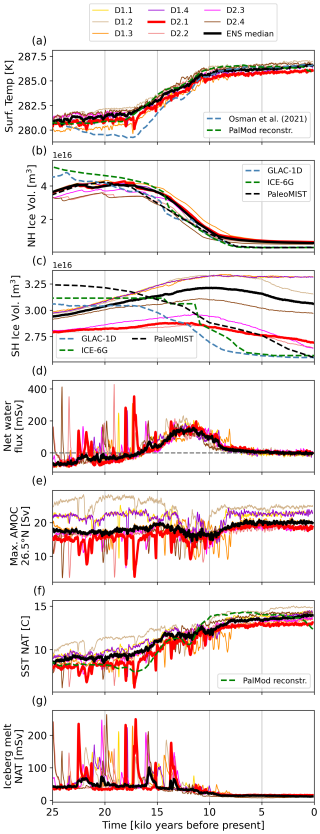
Figure 8 Time series of global mean (a) near-surface air temperature, ice volume in the (b) Northern Hemisphere and (c) Antarctica, (d) net freshwater flux into the ocean, (e) strength of the AMOC at 26.5° N, (f) average SST of the North Atlantic (north of 30° N), and (g) iceberg meltwater flux into the North Atlantic for the model ensemble. The ensemble median is plotted with a thick black line. Model data shown are 100-year running means for climate model variables. Ice-volume data are derived from snapshots 50 years apart. Observational estimates are plotted in the time resolution given by the original data sets. The data from the PalMod reconstructions are anomalies relative to PI. They were transformed into absolute values by adding the last value from the ensemble median.

The latitudinal distribution of the deglacial ocean surface warming signal is shown in Fig. 9 by comparing the sea-surface temperatures (SSTs) over different latitude bands derived from our ensemble to proxy-based estimates. Similar to the global SAT evolution, the SST evolution in the northern extratropics shows a continuous warming throughout the entire simulation, interrupted by several abrupt cooling events. Thereby, the model spread of the transient signal is about 1 K if the abrupt cooling events are excluded (see Fig. 9). A slow warming trend is present at all latitudes until 17 ka, after which the warming significantly accelerates. In contrast, both proxy-based data sets show a temperature minimum around 17 to 16 ka, at the time of H1, followed by rapid deglacial warming which tapers off between 14 and 13 ka.

In the proxy data set, the YD cold event peaks between 13 and 12 ka. A similar cooling signal is also modelled in some of the runs (e.g. D1.1, D1.2 and D1.4), albeit with a weaker amplitude than in the reconstructions. In general, the timing of the occurrence of individual abrupt events varies between the model runs. From 12 ka onward, all curves show a strong warming until the beginning of the Holocene. Hereby, the modelled warming rates are lower than suggested by the proxy data. During the Holocene, the model runs indicate a weak warming trend, in accordance with the Osman et al. (2021) estimate.

In the tropics, the model simulations show a glacial cooling amplitude that is sandwiched by the proxy data, whereupon the PalMod reconstructions indicate less cold SSTs and the reanalysis of Osman et al. (2021) indicates cooler SSTs. The onset of the deglacial warming is overall delayed by approximately 1 kyr. The simulated warming signal at this time is much smoother, and the millennial-scale variability seen in the Northern Hemisphere extratropics is much reduced. While this is in accordance with the reconstructions from PalMod, the Osman et al. (2021) reanalysis shows a temporal variability rather similar to the northern extratropics. In addition, during the early phase of the deglacial warming, the model ensemble is slightly colder than the uncertainty range from the PalMod reconstructions.

In the Southern Hemisphere extratropics, the model simulations agree very well with the reanalysis data by Osman et al. (2021) and lie within the uncertainty range of the PalMod proxy data. All data sets show a slight warming trend through the glacial period. The deglacial warming starts between 18 and 17 ka. The amplitude of the millennial-scale variability is relatively small compared to the other latitude bands. After 11 ka the mean SST in this latitude belt remains stable, which is also indicated by the proxy data (Fig. 9c).

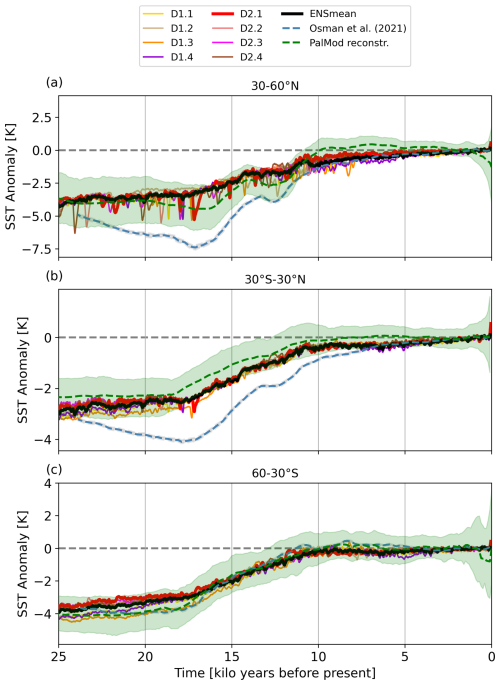
Figure 9 Time series of SST anomalies relative to the PI period for different latitude belts: (a) for the northern mid-latitudes, (b) for the tropics, and (c) for the southern mid-latitudes. Beside our model ensemble, SSTs from the PalMod reconstructions (green; see Appendix A2) and the reanalysis of Osman et al. (2021, blue) are shown (see also Fig. 2). The shading indicates uncertainty estimates, as derived by the PalMod reconstructions. All data were regridded onto a 0.5° grid before averaging over each latitude band. Note that the data frequency differs: Osman et al. (2021) provide 200-year means of annual SSTs, the PalMod reconstructions provide data with a temporal resolution of 100 years, and our ensemble is shown as 100-year running means calculated from decadal mean data.

3.2.3 Ice sheets

At around 25 ka, the simulated Northern Hemispheric ice volume is lower than the ice volume in the ICE-6G (Peltier et al., 2015) and GLAC-1D (Tarasov et al., 2012; Briggs et al., 2014) reconstructions (Fig. 8b) but matches well with the estimate from the more recent PaleoMIST (Gowan et al., 2021) reconstruction. The discrepancy in ice volume between the simulated and the ICE-6G and GLAC-1D ice sheets originates from the overall thinner simulated ice sheets at the beginning of the simulation, primarily in the central ice-sheet regions. The maximum ice volume for ICE-6G and GLAC-1D occurs around 25 ka, followed by a steady ice-volume decrease. The same time period in our simulations is characterized by an ice-volume gain, as is also shown by the PaleoMIST reconstruction. The long-term mass gain is only interrupted by repeated surge events. The growth of the ice sheet is directly related to the continuously low greenhouse gas concentrations prior to 21 ka, resulting in rather cold climate conditions (Fig. 8a). In our simulations and the PaleoMIST reconstructions, the simulated maximum ice volume is typically reached at around 18 ka. At this time, the GLAC-1D reconstruction lies also well within our ensemble spread, whereas the ICE-6G reconstruction indicates larger ice volumes than all model realizations. After 18 ka, ice-sheet volume slowly decreases in our simulations, transitioning into the last deglaciation, with the strongest ice-volume loss occurring between 14 and 10 ka. Ice-volume loss tapers off markedly after 8 ka. At PI, our simulations overestimate ice volume in the Northern Hemisphere by 42 %–47 % in comparison to the reconstructions. The main reason for this is the slow melting of the additional ice caps present in eastern Siberia and over Baffin Island (Fig. 7, second column).

Ocean mixing has a considerable effect on the timing and duration of the deglaciation. Enhanced background mixing in D1.2 leads to a faster decay of the Northern Hemisphere ice sheets compared to D1.1; reduced mixing on the other hand delays the decay (see Fig. 8b and d). Higher vertical mixing enhances Atlantic heat transport in the North Atlantic (not shown), which in turn leads to a warmer climate (compare experiments D1.3, D1.1, and D1.2 in Fig. A1) favouring ice-sheet melt.

As for the Northern Hemisphere, the simulated ice volume in the Southern Hemisphere is lower than indicated by the ice-sheet reconstructions at the beginning of the simulation at 25 ka (see Fig. 8c). While all reconstruction show either constant ice volume or a slight decrease after 25 ka, our simulations exhibit an ice-volume gain until 12–10 ka. Most of our model simulations show an ice-volume decrease only afterwards. However, the magnitude of the ice-volume loss is not large enough over the remaining simulation period, resulting in an Antarctic ice sheet that is too extensive and for which the grounding-line positions are too advanced for PI. Overall, the simulated and reconstructed ice-volume evolution does not match with reconstructions as well as for the Northern Hemisphere. In particular, the advance and retreat magnitudes of the simulated Antarctic ice sheet are underestimated and do not show enough fidelity. As the signals arising from changes in the Antarctic ice sheet are rather small, they did not have an obvious effect on the simulated climate signals during the deglaciation.

3.2.4 Net freshwater flux into ocean

The net water flux into the ocean (Fig. 8d), which on centennial mean timescales is almost identical to the time derivative of the mass of the terrestrial ice sheets, aligns with the growth of the Northern Hemisphere ice sheets during the last part of the glacial. This growth is interrupted by strong discharge events on millennial timescales. From 17 ka onward, the net water flux remains largely positive as a result of the ongoing decay of the ice sheets, with melt rates (direct meltwater discharge as well as melting icebergs) larger than 0.1 Sv between 14 and 10 ka. At the end of the deglaciation, around 8 ka, the ice-sheet mass loss and hence the net water flux reduces drastically and stays relatively constant through the entire Holocene.

From sea-level reconstructions at Barbados, Fairbanks (1989) showed the existence of two meltwater pulses. For the first one, MWP1A, Deschamps et al. (2012) estimated melt rates larger than 0.46 Sv for more than 300 years. MWP1A coincides with the rather warm BA period. Ice-sheet reconstructions such as ICE-6G and GLAC-1D suggest that most of the meltwater was discharged into the North Atlantic or Arctic Ocean. None of our coupled simulations produces an amount of meltwater similar in magnitude to MWP1A around 14 ka. However, meltwater pulses close to 0.4 Sv do occur in our simulations during some of the abrupt events. The existence of the second meltwater pulse, MWP1B, before 11 ka was questioned by Bard et al. (2010) based on sea-level reconstructions from the tropical Pacific. It is not simulated by our model either.

3.2.5 AMOC

The time series of the maximal strength of the AMOC cell at 26.5° N shows marked millennial-scale variability during the glacial period (Fig. 8e). The spread between the ensemble members is considerable. Most simulations show a strengthening of the AMOC from the glacial to the late Holocene. However, there are also simulations with a rather small change in the AMOC between LGM and PI and one simulation (D1.2) with a stronger AMOC at the LGM than at the PI. During the peak of the deglaciation, all simulations show a weakening of the AMOC, which we explain as the response to meltwater hosing, enhancing vertical stability and reducing the ventilation of the deep-water masses. The slow warming in response to rising greenhouse gas concentrations further amplifies vertical stability. Except for short periods of time, the model AMOC is always in a strong mode.

4 Abrupt events

The transient climate evolution of the past 25 ka is interrupted by several abrupt events. For each of our ensemble members, these abrupt events occur at very different times during the glacial and the deglaciation. Here, we focus on the deglacial key events, which are related to changes in the AMOC. To examine the drivers of the abrupt events, we first focus on simulation D2.1. Figure 10b shows the time evolution of the AMOC and the dye fraction over depth at 26.5° N. The overall trend of a strengthening and deepening of the AMOC cell from the glacial to the Holocene is interrupted by numerous abrupt events, which are accompanied by strong signals in the dye fraction and indicate water mass displacements throughout the whole water column (see also Fig. A4). A close relationship between changes in the net freshwater flux (Fig. 10a) and variations in AMOC and the dye fraction profile is visible.

In the following we will examine individual abrupt events and discuss the underlying mechanisms. Based on our simulations, we can distinguish between three different mechanisms behind the simulated abrupt cold events: HE-like surges from the Northern Hemispheric ice sheets and events that are triggered by changes in the Arctic net freshwater budget or a river rerouting over North America.

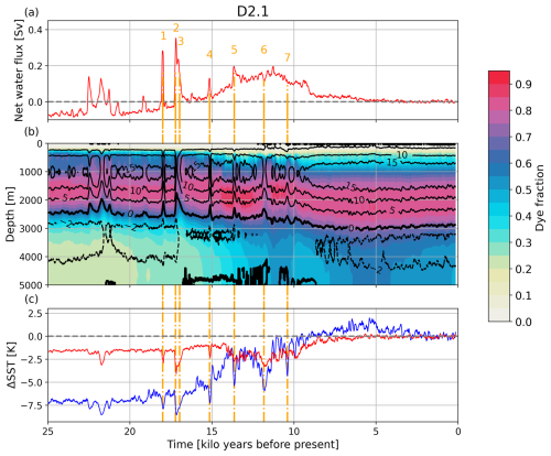
Figure 10 (a) Time series of the global freshwater input into the ocean; (b) a time–depth plot of the AMOC at 26.5° N superimposed on the zonally averaged fraction of water originating from the surface of the North Atlantic and Arctic; and (c) SST anomaly time series at 54° N, 30° W in the subpolar (blue) and 38° N, 46° W in the subtropical (red) North Atlantic for ensemble member D2.1. Orange dashed–dotted lines and orange numbers in panel (a) mark specific AMOC weakening/North Atlantic cooling events discussed in the text. Contour lines in panel (b) are at −2, 0, 5, 10, and 15 Sv. The thick black line between 2000–3000 m indicates the lower boundary of the NADW cell (AMOC =0 Sv). Data shown are 100-year running means.

4.1 Drivers of abrupt climate events during the last deglaciation

4.1.1 HE-like surge events

The first deglacial meltwater peak in D2.1 occurs around 18.0 ka (event 1 in Fig. 10a). The snapshot maps (see Fig. 11a) show that the event at this time is caused by a surge event from the Fennoscandian ice sheet, with massive iceberg discharge into the Norwegian Sea. This enhances iceberg melt in the Nordic Seas and the North Atlantic. The meltwater reduces surface salinity, suppresses deep convection, and consequently leads to a weakening of the AMOC and an upward shift of the margin between AABW and NADW (Fig. 10b). These changes are accompanied by a surface cooling in the North Atlantic (see Figs. 10c and 8f). Note that the SST cooling in the subpolar and the subtropical North Atlantic associated with AMOC weakening events is of similar magnitude during the glacial and early deglaciation (Fig. 10c). The glacial temperature at the subpolar location is already rather close to freezing point, which very effectively limits the potential amplitude of any cooling signal at this location.

The next meltwater peak, occurring around 17.22 ka (marked as 2 and 3 in Fig. 10a), is caused by surges from the Laurentide ice sheet (Fig. 11b). The event consists of two almost synchronous surges from two source regions of the Laurentide ice sheet. First, a surge in the western part of the Laurentide towards the Arctic occurs. While this surge slows down, another surge takes place from the eastern Laurentide through the Hudson Strait (Fig. 11c). This abrupt event is rather strong, with a weakening of the AMOC down to 3.9 Sv at 17.2 ka (as indicated in the 100-year means in Figs. 10b and 8e). As a result, the margin between the NADW and the AABW cells shifts upward by approx. 800 m. The depth of the 70 % NADW dye fraction moves upward and reaches a maximal uplift of about 400 m 200 years later. The two surges combined discharge a water equivalent of almost 8 m of global sea level within 450 years. This is within the previously reported range for HEs of 2–20 m over a time period of 500 years (Hemming, 2004; Roche et al., 2004; Roberts et al., 2014).

The next event, at approximately 15.14 ka (marked as 4 in Fig. 10a), is again caused by a discharge event from the Fennoscandian ice sheet into the Norwegian Sea (Fig. 11d). It is followed by the last big iceberg discharge event around 13.64 ka (event 5 in Fig. 10a) from the eastern Laurentide ice sheet through the Hudson Strait (see Fig. 11e). As the deglacial warming is already ongoing during these two events and the temperature at the subpolar location is now well above the freezing point, the SST cooling signals in the subpolar location are now stronger than in the subtropics, similar to the responses known from typical PI hosing experiments (e.g. Schiller et al., 1997; Stouffer et al., 2006; Smith and Gregory, 2009).

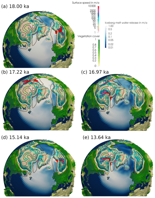
Figure 11 Snapshots of different surge events from the Northern Hemisphere ice sheets during the last deglaciation for simulation D2.1. The movie of the entire deglaciation is available under https://doi.org/10.5446/69659 (Ziemen et al., 2024). Colours on the ice sheets indicate the surface speed, colours on land indicate maximum vegetation cover, and colours in the ocean indicate the amount of iceberg meltwater release. Isolines indicate the vertical displacement of the bedrock relative to the end of the simulation. Black isolines indicate depressed bedrock, and brown isolines indicate elevated bedrock as compared to PI. No change is indicated by a white isoline. The spacing between individual contours is 100 m, with the exception of the ± 50 m contour.

4.1.2 Events not caused by ice surges

After 13.64 ka, the North Atlantic in D2.1 shows two more distinct SST cooling events (marked as 6 and 7 in Fig. 10). The first of these events reaches a temperature minimum around 11.83 ka and the other one at 10.4 ka in simulation D2.1 (Fig. 10c). They coincide with a significant decrease in the maximum AMOC strength (Fig. 10b). But, unlike the previous events, they cannot directly be associated with an abrupt increase in the total amount of meltwater and/or iceberg discharge from the Laurentide or Fennoscandian ice sheets (Fig. 10a).

Sign shift in the Arctic net freshwater balance

The first of these two cold events takes place during the peak of the deglaciation (event 6 in Fig. 10a). During this time, the Laurentide and Fennoscandian ice sheets experience significant mass loss in response to the increase in global temperatures and summer insolation. This is indicated by an increase in global meltwater release (Fig. 10a), which is most pronounced in the Arctic (Fig. 12b). This meltwater input into the Arctic leads to a regime shift in the net freshwater budget of the Arctic Ocean. This quantity is defined as the balance between the meteoric freshwater input (river runoff, precipitation, and iceberg melt minus evaporation) and the export of sea ice from the Arctic into the adjacent seas, which represents a measure for the integrated net freezing rate of Arctic sea ice and the associated brine release. During the glacial period, the Arctic sea-ice export and thus the brine release dominates over the meteoric freshwater input. Hence, the water leaving the Arctic has a higher salinity and colder temperatures and is therefore denser than the inflowing water of Atlantic origin. As a consequence, it contributes to the formation of NADW. Due to the increase in meltwater input from the Laurentide ice sheet into the Arctic Ocean, the net freshwater budget becomes positive for the first time at about 12.47 ka. This means that the Arctic transitions from a state with an effective net freshwater loss due to sea-ice formation and export to a state with a positive net freshwater budget (Fig. 12b). While this transition occurs rather gradually and takes until about 11.78 ka to be completed in D2.1, it allows for an abrupt decrease in the surface salinity in the Arctic, as the positive net freshwater input allows for a halocline to develop. This stabilizes the stratification in the Arctic and suppresses deep convection in the Arctic. Furthermore, the water leaving the Arctic is now fresher and less dense than the inflowing water. The resulting reorganization of the NADW formation leads to a decrease in AMOC strength. At first the AMOC weakening is rather gradual and overlaid by large centennial-scale variability. The gradual decrease in Arctic sea-ice export starting at about 12.0 ka results in a further increase in the net freshwater budget and ultimately leads to an abrupt weakening of the AMOC (Fig. 12c).

The overall increase in sea level and the retreat of the ice sheets result in the opening of the Bering Strait and the Barents Sea Opening at about 11.37 and 11.18 ka, respectively. Here, we use the term Barents Sea Opening for the gateway between Svalbard and continental Europe, enabling throughflow between the Norwegian Sea and the Arctic. The opening of the Bering Strait leads to a considerable reduction of Arctic sea-ice volume (about 20 %) and results in a net export of freshwater into the Pacific (not shown). The opening of the Barents Sea Opening further allows for additional sea-ice export to the Nordic Seas (about 20 %). Hence, the opening of both straits ultimately increases the surface salinity in the Arctic, which decreases the stable stratification, enhances the deep-water formation, and allows for an increase in the AMOC strength to nearly pre-event values. Note that the AMOC recovers slightly before the abrupt salinity increase in the Arctic in response to the opening of the Bering Strait. This increase can likely be attributed to a substantial centennial to millennial variability of the AMOC (see Fig. 12a and c).

It is noteworthy that the freshwater input into the Nordic Seas increases rather rapidly around the time of the opening of the Barents Sea Opening at 11.18 ka. This increase is associated with a redirection of meltwater from the southern margin of the Fennoscandian ice sheet. Relatively small changes in the land–sea mask and ice-sheet margin allow for a redirection of these waters from the North Sea towards the northeast into the White Sea and eventually into the Barents Sea, causing an abrupt increase in the freshwater input into the Nordic Seas (see Fig. 12b) and reduction in Nordic Seas surface salinity.

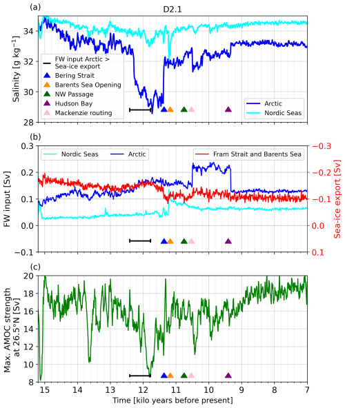
Figure 12 Time series of the (a) surface salinity in the Arctic (blue) and Nordic Seas (cyan) and (b) freshwater input into the Arctic (blue) and Nordic Seas (cyan), both derived from precipitation minus evaporation, river runoff, and iceberg melting as well as the Arctic sea-ice export through the Fram Strait and Barents Sea Opening (red; right axis) in simulation D2.1. (c) Time series of the maximum AMOC strength, as presented in Fig. 8d. All data are shown as decadal means. The black bar indicates the sign shifts of the Arctic freshwater budget, whereby the time range shows when the decadal surface freshwater budget of the Arctic becomes positive for the first time and negative for the last time. The triangles mark the opening of the major Arctic Ocean gateways, namely the Bering Strait (blue), the Barents Sea Opening (orange), the Northwest Passage (green), and the Hudson Bay (purple). The change in river routing that allows for enhanced freshwater input through the Mackenzie River into the Arctic Ocean is indicated in pink.

Changes in river routing

The second of the non-surge-induced cooling events (about 10.4 ka; event 7 in Fig. 10) is driven by a redirection of meltwater from the Laurentide ice sheet. At this time, much of the meltwater from the Laurentide ice sheet is routed through the St. Lawrence or Mackenzie rivers and ends its path either in the North Atlantic or Arctic, respectively. The paths of the two rivers follow the southern edge of the Laurentide ice sheet and are separated by a drainage divide located northwest of today's Great Slave Lake (Fig. 13a). At about 10.49 ka, the continued retreat of the northwestern part of the Laurentide ice sheet in conjunction with changes in the land topography through glacial isostatic adjustment allows for the Mackenzie drainage basin to extend much further southeast, all the way towards the Great Lakes (Fig. 13b). This rerouting leads to a redirection of approximately 0.08 Sv of meltwater from the St. Lawrence River to the Mackenzie River and results in an abrupt increase in meltwater discharge into the Arctic (Fig. 12b). The freshwater is transported through the coastal boundary currents of the Arctic Ocean towards the deep-water formation sites in the Greenland and Labrador seas, where it leads to a reduction of the NADW formation and thereby a weakening of the AMOC.

The enhanced discharge of meltwater into the Arctic lasts until about 9.41 ka. At this time, the Laurentide ice sheet collapses and splits into two small ice sheets on Baffin Island and in southeast Canada. The associated changes in sea level and glacial isostatic adjustment lead to the opening of the Hudson Bay (Fig. 12) and allow for a rerouting of water into the Hudson Bay (Fig. 13c). A consequence of the ice-sheet collapse is a short increase in the release of icebergs and their melt into the North Atlantic (Fig. 8g). In response to these changes in the river routing, the AMOC recovers and slowly increases towards its modern strength.

Figure 13 Snapshots of the river discharge and their catchments for a time slice before and after the change in the river routing that triggers the 10.4 ka cooling event in D2.1 and after the Hudson Bay opening in the ocean model. Shown is the river discharge through the main rivers (colour bar) over North America at (a) 10.52 ka, (b) 10.47 ka, and (c) 9.25 ka together with the main catchment areas, indicated by the coloured overlays. Note that several catchments are combined in one colour: shown are all catchments that discharge into the Arctic (green), the Baffin Bay and Labrador Sea (orange), the North Atlantic and Nordic Seas (purple), the southern North Atlantic (blue), and the Pacific (pink). The grey background shading marks the land–sea mask on the ocean model grid. White hatching marks the glacier mask, as obtained from the ice-sheet model.

Table 2 Timing of the opening of the Arctic straits and the change in the river routing favouring enhanced discharge through the Mackenzie River (in ka). All events are marked by triangles and the black bar in Fig. 12. Values for ICE-6G_P3 and GLAC-1D_P3 are taken from transient deglacial simulations with prescribed ICE-6G and GLAC-1D ice-sheet reconstructions, respectively (see Kapsch et al., 2022). A deviation from the bold font indicates that the opening is more than 1000 years earlier (regular) or later (italic) than the range given by proxy evidence.

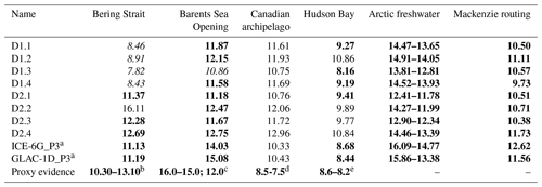
^a Kapsch et al. (2022). ^b Elias et al. (1996); Dyke and Savelle (2001); Keigwin et al. (2006); England and Furze (2008); Jakobsson et al. (2017). ^c Hughes et al. (2015); Rovira-Navarro et al. (2020). ^d England (1999); England et al. (2006). ^e Tarasov et al. (2012).

4.2 Abrupt events in the ensemble

In this subsection we discuss how robust the mechanisms that we have found in the previous subsection are. For this we now discuss the entire ensemble. All ensemble members show abrupt millennial-scale events (see Fig. 8) similar to the events presented for D2.1. Abrupt AMOC weakening events lead to a strong cooling in the North Atlantic SST of several kelvin. Many of these events also show large pulses of iceberg melting in the North Atlantic, indicative of HE-like surge events. Hence, we will distinguish in the following between HE-like surge events, abrupt events induced by a persistent sign shift in the Arctic net freshwater balance, or changes in the river routing.

4.2.1 Abrupt events due to HE-like surges

HE-like surges are caused by internal variability of the Northern Hemisphere ice sheets in our model system (Ziemen et al., 2019; Schannwell et al., 2023, 2024), which largely follows the classic binge–purge mechanism suggested by MacAyeal (1993). However, the timing of these events is highly variable as shown by the considerable spread between the ensemble members. As the external forcing (orbital parameters and atmospheric greenhouse gas concentrations and for a subset of our ensemble also the volcanic forcing) is identical in all simulations, it cannot serve as explanation for the difference in the timing of the events. As all asynchronous spin-up simulations started from the same state at 45 ka, model parameters obviously have an effect on the timing of the surge events.

To test the role of initial conditions, two additional sensitivity experiments have been performed. These simulations are identical to D2.1, except for slight differences in the initial fields for the ice-sheet and solid-earth model. Instead of the 26 ka conditions, we used the ice-sheet and solid-earth conditions from 27 ka (D2.1.1) and 28 ka (D2.1.2) in the asynchronous spin-up as the initial state. Together with D2.1, the simulations D2.1.1 and D2.1.2 thus allow us to investigate the effect of the initial state of the ice sheet on the timing of the surge events. Of our three main surge regions, the Hudson Strait tends to show the most regular interval between individual events, suggesting a higher predictability of surge events than the other regions. D2.1.1 and D2.1.2 simulate Hudson Strait surge events that are offset by 1 and 2 kyr (Fig. 14a), which matches the shift in the initial state of the ice sheets and corroborates a high level of predictability shown in previous studies (Schannwell et al., 2023, 2024). In agreement with these studies, the level of predictability is considerably lower for the surges originating from the western Laurentide ice sheet. For this region, the spread in the timing and strength of the events is much more irregular, and the simulated shifts in D2.1, D2.1.1, and D2.1.2 are closer to 1 ky instead of the expected 1 and 2 ky (Fig. 14b) from the initialization. The predictability for our third surge region, the Fennoscandian ice sheet, lies somewhere in between the predictability of the other two surge regions (Fig. 14c). Overall, our sensitivity simulations clearly demonstrate the importance of the initial conditions for the timing of the surge-induced abrupt events.

Furthermore, the simulated climate over the ice sheets (especially surface mass balance and surface temperature) has an effect on the timing and frequency of the surge events (Schannwell et al., 2023, 2024). Together with the rather chaotic surge behaviour of the Mackenzie ice stream, this further enhances the stochastic contribution in the timing of the surge events. Both the initial conditions and the choice of the model parameters influence the timing of the surge event. In consequence, the exact timing of surge-type variability, as derived from observations, cannot be reproduced by a model with interactive ice sheets.

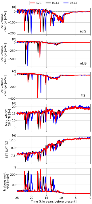
Figure 14 Change in ice volume for (a) the eastern Laurentide (eLIS), (b) the western Laurentide (wLIS), and (c) the Fennoscandian (FIS). (d) The strength of the AMOC at 26.5° N; (e) the average SST of the North Atlantic; and (f) the iceberg meltwater flux in the North Atlantic for simulations D2.1, D2.1.1, and D2.1.2.

4.2.2 Late deglacial abrupt events

The last two North Atlantic cooling events in D2.1, which are not associated with the occurrence of HEs, can also be identified in most other ensemble members (Fig. 8e, f). While the timing of the individual events differs between ensemble members, the processes leading to abrupt events in D2.1 are similar in all ensemble members.

Sign shift in the Arctic net freshwater balance

In most of our simulations, the onset of the first event not induced by ice-sheet surges is associated with the transition into a regime in which the net freshwater input into the Arctic becomes larger than the sea-ice export to the North Atlantic. This leads, similar to D2.1, in all simulations to the formation of a halocline in the Arctic and a significant reduction in the AMOC strength. However, the timing of the transition towards a positive net freshwater input into the Arctic varies between simulations. Therefore, the timing at which the AMOC strength significantly reduces also differs across ensemble members. For example, D2.2 and D2.3 show weaker AMOC slowdowns and North Atlantic cooling during the onset of this abrupt cooling event than the other simulations. This is likely related to the Bering Strait being open already before the event, at 16.11 ka in D2.2 and 12.28 ka in D2.3 (see Table 2), ultimately influencing the freshwater balance by sea-ice export to and the inflow of saltier water from the North Pacific. This is in line with Karami et al. (2021), who showed that the Arctic gateways can have a different impact on the ocean dynamics in the Arctic, depending on whether the Bering Strait or Canadian archipelago are closed or open. Our findings are also in agreement with findings by Hu et al. (2012), who showed that abrupt AMOC transitions are more likely when the Bering Strait is closed. In accordance with Hu et al. (2012), we find that the simulations that exhibit a late opening of the Bering Strait show stronger variations in the Arctic Ocean and AMOC in response to the shift of the sign in the net freshwater balance than the simulations with an early opening.

In our simulations the Bering Strait also plays a pivotal role towards the end of the abrupt event initiated by the changes in the freshwater budget of the Arctic. As shown for D2.1, the opening of the Bering Strait leads to a recovery of the AMOC through an increase in salinity of the Arctic and, thus, a decrease in the vertical stability (see Sect. 4.1). This is the case for all but one of the ensemble members. In line with Karami et al. (2021), who found that the opening of the Bering Strait leads to a substantial salinity increase in the top 50 m of the Arctic Ocean, our simulations show a substantial increase in surface salinity for D2.1 (Fig. 12b) and the majority of our simulations (D1.1, D1.2, D1.3, D1.4, D2.3, D2.4, not shown). We find that part of this increase in surface salinity can be attributed to a net export of freshwater through the Bering Strait into the Pacific (not shown), which is in agreement with findings by Hu et al. (2008). As the timing of the Bering Strait opening varies significantly between simulations, the full recovery of the salinity also varies. For the simulations with a late opening of the Bering Strait (D1.1, D1.2, D1.3, D1.4), the Arctic is able to maintain low surface salinity and thereby its stable halocline over several millennia. This leads to an overall weaker AMOC with substantially higher variability throughout the course of the deglaciation, until the Bering Strait finally opens (see Table 2).

It is noteworthy that the ocean response to an opening/closing of the Bering Strait differs from other studies in some aspects. For example, Hu et al. (2015) argue that the opening/closing of the Bering Strait has a substantial impact on the sign of the freshwater budget in the Arctic. They find that if the Bering Strait is opened under deglacial conditions (15 ka), the Arctic changes from a freshwater sink to a freshwater source. Our simulations do not show such a relationship. Rather, they show a transition from a typical glacial state, where the sea-ice export from the Arctic to the Atlantic is larger than the freshwater input into the Arctic, to a state where the freshwater input is larger. Further, our simulations show that this transition is an inherent transient climate response that occurs in all simulations independent of when the Bering Strait is opening. The main difference between the experiments from Hu et al. (2015) and our simulations is that an opening of the Bering Strait in our simulations leads to reduced sea-ice export from the Arctic to the Atlantic, whereas their model simulates an increased export. In our simulations, the reduced ice transport is also a result of a reduced sea-ice volume inside the Arctic. These differences are likely related to Hu et al. (2015) not considering the effect of freshwater release by melting ice sheets.

A similar sign shift of the Arctic freshwater budget and transition into a slightly weaker AMOC state is also evident in simulations with prescribed ice sheets (Kapsch et al., 2022) from the ICE-6G (Peltier et al., 2015) and GLAC-1D reconstructions (Tarasov et al., 2012) starting at about 16.09 and 15.86 ka, respectively (see also Table 2). The transition from a state where sea-ice export to the Atlantic is larger than the freshwater input into the Arctic to a state where the freshwater input dominates is accompanied by the development of a halocline in the Arctic Ocean in the simulations with ICE-6G and GLAC-1D reconstructions (see ICE6G_P3 and GLAC1D_P3 in Table 2). However, the AMOC response in these simulations is much weaker than in the fully coupled simulations (not shown). This is likely related to a relatively low prescribed meltwater input into the Arctic, which was derived from the ice-sheet reconstructions during this time. Only around the time of MWP1A does the freshwater input significantly increase. In general, the simulations with coupled ice sheets show an earlier and more gradual increase in freshwater during the peak of the deglaciation, while the freshwater input into the ocean in the simulations with prescribed ice sheets is dominated by pulses of meltwater. This likely explains the different response.

Changes in river routing

The deglacial North Atlantic cooling event that is associated with enhanced river discharge into the Arctic due to changes in the river routing also occurs in all our ensemble members (see Table 2). It is, consistent with D2.1, in all simulations associated with an expansion of the drainage basin of the Mackenzie River and accompanied by an AMOC slowdown. It agrees with simulations by Kapsch et al. (2022), where ice-sheets from the ICE-6G reconstructions were prescribed, as well as studies by Tarasov and Peltier (2005) and Condron and Winsor (2012), who indicate that a rerouting of rivers caused the YD cooling. Using a high-resolution ocean–sea-ice model, Condron and Winsor (2012) show that freshwater discharged from the Mackenzie River is transported through the narrow coastal boundary currents towards the deep-water formation sites in the Greenland and Labrador seas, where it disrupts the open-ocean convection and thereby weakens the AMOC. In our simulations, the expansion of the Mackenzie drainage basin, due to a small retreat on the southern edge of the Laurentide ice sheet, leads to an abrupt increase in the freshwater input into the Arctic and, thereby, triggers the simulated AMOC slowdown and accompanying Northern Hemispheric cooling consistent with D2.1. In all simulations, the collapse of the Laurentide ice sheet and the opening of the Hudson Bay, which allow for a rerouting of the meltwater previously entering the Arctic Ocean to the Hudson Bay (Fig. 13), lead to a recovery of the AMOC. The freshwater reaching the Labrador Sea through the Hudson Strait flows southeastward in a coastal current and has therefore a relatively small effect on the deep convection in the Labrador Sea. Interestingly, the timing of the change in the river routing occurs in some ensemble members before the opening of the Bering Strait (D1.1, D1.2, D1.3, D1.4), hence in a state where the salinity in the Arctic is already reduced and the stratification is relatively stable. Despite this, all simulations show a distinct AMOC weakening in response to the enhanced Arctic freshwater input, indicating that the process itself is consistent throughout all ensemble members (not shown). The results emphasize that changes in the river routing played a crucial role in initiating the North Atlantic cooling events that occur in our simulations between about 12 and 9 ka (Fig. 8). Further, the AMOC recovery that follows the opening of the Hudson Bay indicates the importance of changes in the land–sea mask in response to the ice-sheet collapse and associated deglacial sea-level rise for the occurrence of abrupt events. As the changes in river routing and the opening of the Hudson Strait are in all simulations related to the gradual retreat of the Laurentide ice sheet, they appear to be deterministic and, hence, seem to be an integral part of the deglaciation.

5 Summary and conclusion

We have applied the newly developed coupled atmosphere–ocean–vegetation–ice-sheet–solid-earth model MPI-ESM/mPISM/VILMA to the last deglaciation. Topography and river-routing directions are calculated according to the simulated states of ice sheets and solid earth. By prescribing time-varying atmospheric greenhouse gas concentrations, earth orbital parameters, and – in most runs – a volcanic forcing as the only time-dependent forcings, the coupled model is able to simulate a realistic deglaciation including abrupt millennial-scale climate events. Through an ensemble of eight simulations, we show that the simulated climate change between the LGM and PI and the simulated deglaciation is sensitive to the prescribed model parameters, particularly to the vertical background mixing in the ocean. The simulated SST anomaly between the LGM and PI of all simulations is in line with reconstructions based on proxy data. Nearly all ensemble members show a shallower, and at most a slightly weaker, NADW cell during the LGM than during PI. Interestingly, estimating the shallowing of the NADW cell from changes in the distribution of a proxy-like water mass tracer (artificial dye tracer) indicates a stronger signal than the values derived directly from the simulated AMOC. This demonstrates an additional methodological challenge in estimating past AMOC changes from sediment proxy records.

All ensemble members show abrupt cooling events. For glacial periods and during the early deglaciation, these events are caused by surges from the Laurentide and Fennoscandian ice sheets that result in the release of a huge number of icebergs into the North Atlantic, the Nordic Seas, and the Arctic. The resulting meltwater input into the ocean leads to reduced surface salinity, suppressed formation of deep water, and a weakened AMOC. After the end of each surge event, the system recovers to its previous state. This HE-like variability represents a glacial mode of internal climate variability of the coupled model system. However, the timing of the simulated HE-like surge events shows a considerable scatter in the model ensemble. Additional sensitivity experiments confirm that these events are not entirely determined by the prescribed external forcing but that the initial conditions – especially of the Northern Hemispheric ice sheets – as well as the model parameters play an important role for the timing of these events. Except for the relatively short AMOC weakenings, the simulated AMOC in our model is always in a strong mode, indicating a mono-stable AMOC. Performing similar experiments using a model system which simulates a weak AMOC mode for glacial climates like Obase and Abe-Ouchi (2019) might yield a rather different time evolution of the AMOC.

The glacial climate of the Arctic in our model system is characterized by sea-ice export to the Atlantic that exceeds the amount of freshwater input to the Arctic through river runoff, iceberg melting, and precipitation minus evaporation. This effectively prevents the development of a stable halocline and causes the formation of water masses that are colder, saltier, and denser than the inflowing water of North Atlantic origin. During the deglaciation, the enhanced meltwater input due to melting ice sheets together with precipitation and river runoff exceeds the amount of freshwater that is leaving the Arctic through sea-ice export. The transition towards a positive net freshwater balance leads in all simulations to the formation of an Arctic halocline. This results in the suppression of dense water formation within the Arctic and a weakening of the AMOC that is accompanied by a cooling in the North Atlantic realm. While the halocline emerges relatively abruptly in most simulations, it depends on the overall state of the Arctic Ocean, which in turn is controlled by the import and export of waters from the adjacent seas through the major straits (specifically the Bering Strait). As the timing of the opening of those passages differs between simulations, the magnitude and abruptness of the AMOC response differ as well.

Additionally, river rerouting in connection with the opening of the Hudson Bay can cause abrupt changes in AMOC and North Atlantic climate. These processes become particularly relevant when the size of the Laurentide ice sheet is already strongly reduced. The chronological order of the opening of the Bering Strait and the river rerouting thereby substantially affects how abrupt the onset and/or offset of the events is.

In a comprehensive comparison of the glacial and deglacial climate with proxy data, we show that the overall climate trajectory of our ensemble agrees well with observations. The validation of abrupt events in the model with proxy records is not straightforward, especially with respect to the timing of the abrupt events. Although it has been shown that HE-like surge events have a characteristic return period and are to some degree phase-locked to the climate changes (Schannwell et al., 2024), the timing of the abrupt cooling events that are associated with ice-sheet surges in our ensemble is non-deterministic and largely depends on the initial conditions and model parameters. The abrupt events associated with an opening of passages or river rerouting are in principle reproducible as they occur in all ensemble members. However, the nonlinearities involved, such as ice-sheet shape, retreat as glacial isostatic adjustment makes the simulation of the exact timing of these events sensitive to model parameters. Consequently, a temporal matching of the simulated abrupt events with the events derived from proxy data is difficult to achieve. In addition, the dating of proxy records is subject to a high degree of uncertainty. In conclusion, the millennial-scale climate variability in models may not align with timescales found in proxy data, so a validation should rather be based on statistical methods, similar to the model simulations of historical climate with El Niño–Southern Oscillation (e.g. Planton et al., 2021), rather than on the individual timing and strength of deglacial key events.

Our novel model framework presented here is a step towards a better understanding of the processes and interactions between different climate components on deglacial timescales. By including for the first time interactive earth system components such as ice sheets, icebergs, solid earth, and time-evolving river directions and land–sea mask into a comprehensive ESM, we reveal previously unrecognized chains of processes that explain the climate features observed throughout the last deglaciation. While in this paper we mainly focus on the overall deglacial climate response to changes in the external forcing, such as insolation, greenhouse gases, and volcanoes, as well as on the abrupt climate events that occur due to the internal variability of the climate system, our ensemble will enable the analysis of a wide variety of processes in each of the individual modelled climate components and between them. Furthermore, it emphasizes the importance of incorporating earth system components that are traditionally regarded as exhibiting too slow a rate of change to be relevant for transient climate simulations.

Appendix A

A1 Model parameters

A2 PalMod reconstructions

The PalMod reconstructions rely on a synthesis of marine proxy records for temperature of the last glacial cycle, the PalMod 130k marine palaeoclimate data synthesis, beta version 2.0.0 (Jonkers et al., 2020). The database includes globally distributed sea-surface temperature proxies based on alkenone, TEX86, long-chain diol index, Mg $/$ Ca ratios in planktonic foraminifera, and microfossil assemblages. The global mean SAT is computed based on the selection of records and the algorithm described in Baudouin et al. (2025). More specifically, the algorithm is an adaptation of the one used in Snyder (2016) to leverage the potential of the SST record data set fully. At its core, the algorithm aggregates SST records over latitudinal bands to estimate a 60° S–60° N SST anomaly time series. A scaling factor of 1.9, based on an ensemble of LGM simulations (Snyder, 2016), is then applied to derive the global mean temperature. The latitudinal bands and North Atlantic averages are computed by aggregating the records over the specific domain without applying a scaling factor.

A3 Modelled surface temperature bias for PI

The model shows systematic temperature biases for PI when compared to data from the ERA20C (Poli et al., 2016) reanalysis (Fig. A1). This SAT bias appears in all experiments. The climate over northeast North America is too warm, and over Scandinavia and eastern Asia it is too cold. North Atlantic SSTs are too cold (except for the high mixing simulation D1.2). The warm bias around Antarctica is associated with an underestimation of the sea-ice extent. Reduced vertical mixing reduces the bias (D1.3), and enhanced mixing amplifies the bias (D1.2).

Table A1 Individual parameter settings for each model component across the ensemble members and corresponding spin-up simulation. In all asynchronous spin-up simulations climatological volcanic forcing was used.

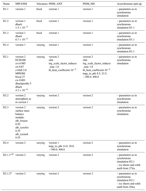
^a The sensitivity studies D2.1.1 and D2.1.2 are not part of the ensemble. ^b D.2.1.1 was run only until 7 ka.

Table A2 List of all parameters and their full name as well as standard value that were varied across the ensemble members.

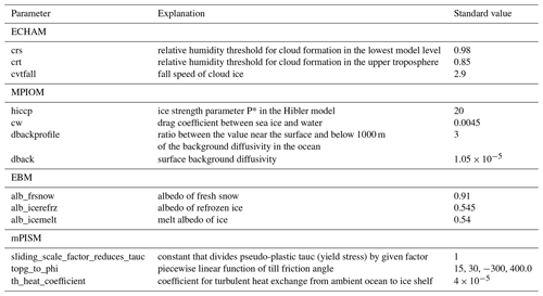
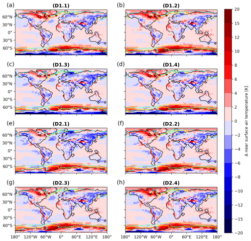
Figure A1 Difference in annual mean near-surface air temperature between model and ERA-20C (Poli et al., 2016) reanalysis (colours, averaged over 1901 to 1955). Panels (a)–(h) show individual ensemble members. The isolines show the sea-ice extent (>0.15 sea-ice coverage in the long-term mean seasonal climatology) from years 1900 to 1955 of the HadISST data set (Hurrell et al., 2008) for summer (solid yellow) and winter (dashed yellow) and from the model for summer (solid cyan) and winter (dashed cyan). The land–sea mask is indicated by the solid black lines.

A4 Effect of vertical mixing on AMOC

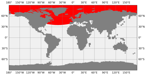
Figure A2 Source function for the NADW dye tracer with 1 (red) in the northern Atlantic and the Arctic and 0 (light grey) at the remaining ocean surface.

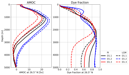
Figure A3 As Fig. 4a and c but for selected ensemble members with different vertical background mixing rates: D1.3 has the lowest rate and D1.2 the highest (see Table A1). Solid lines represent the PI state and dashed lines the LGM state. The data show an average over the periods from 23 to 18 ka and from 1.1 to 0.1 ka. The simulations were started from the same spin-up state at 26 ka.

A5 Temporal evolution of dye fraction on the lower boundary of NADW cell

Sedimentary proxy data have a long tradition of being used to estimate changes in the AMOC strength and geometry (e.g. Duplessy et al., 1988; Oppo and Lehman, 1993; LeGrand and Wunsch, 1995). In addition to methodological uncertainties intrinsic to sediment proxy data (e.g. biologically induced errors in the recording and preservation of the targeted signal, temporal changes in source functions, or measurement errors), the interpretation of the determined variations in terms of changes in AMOC geometry or strength is not straightforward. The dye fraction provides some insights into the temporal evolution of the signal within a consistent model system including a well-defined constant source function at the surface (1 for the northern Atlantic and Arctic surface waters and 0 for the remaining ocean surface, including the Southern Ocean deep-water source regions).

Figure A4 supplements the information given in Fig. 10 and displays the temporal evolution of the zonally averaged dye fraction on the water mass boundary between NADW and southern source deep waters, defined by AMOC =0, for the latitudinal range from 30° S to 40° N over the entire deglaciation. Overall, the dye fraction increases by 0.1 to 0.15 from the LGM to present day at all latitudes, with a larger increase in the Southern Hemisphere when the NADW reaches further south during PI (Fig. 5). It can be assumed that a similar temporal shift occurs in proxy data, which are used to estimates the AMOC geometry. The interpretation of these proxy data might, in turn, lead to a biased AMOC geometry or to the assumption that the source function of the proxy must have changed over time.

Additionally, we find that the latitudinal pattern in the dye fraction does not evolve uniformly over time. In particular, larger variations in the dye fraction are present in the Southern Hemisphere than in the Northern Hemisphere during abrupt events. The reconstruction of Atlantic water mass properties from sediment core data which are distributed over the whole Atlantic north of 30° S could be complicated by this latitudinal modulation of the dye fraction. As already stated in the main text, we do not claim that our dye fraction represents real-world proxy data, but within our consistent model system we find additional sources of uncertainties which might complicate the reconstruction of the AMOC geometry based on proxy data.

Figure A4 Time evolution of the zonal mean dye fraction at the depth of AMOC =0 for latitudes between 30° S and 40° N in simulation D2.1. Data shown are 100-year running means.

A6 Ice volumes at the LGM and PI

Table A3 Ice volumes in ×10¹⁵ m³ of major ice sheets for all simulations at the LGM and PI.