Contrasts in the marine inorganic carbon chemistry of the Benguela Upwelling System since the Last Glacial Maximum

Upwelling regions are dynamic systems where relatively cold, nutrient-, and CO₂-rich waters reach to the surface from the deep. CO₂ sink or source properties of these regions are dependent not only on the dissolved inorganic carbon content of the upwelled waters, but also on the efficiency of the biological carbon pump which constrains the drawdown of atmospheric CO₂ in the surface waters. The Benguela Upwelling System (BUS) is a major upwelling region with one of the most productive marine ecosystems today. However, contrasting signals reported on the variation in upwelling intensities based on, for instance, foraminiferal and radiolarian indices over the last glacial cycle indicate that a complete understanding of (local) changes is currently lacking. To reconstruct changes in the CO₂ history of the northern Benguela upwelling region over the last 27 kyr, we used a box core (64PE450-BC6) and piston core (64PE450-PC8) from the Walvis Ridge. Here, we apply various temperature and pCO₂ proxies, representing both surface (U${}_{\mathrm{37}}^{K^{\prime }}$ and δ¹³C of alkenones) and subsurface (Mg $/$ Ca and δ¹¹B in planktonic foraminiferal shells) processes. Reconstructed pCO₂ records suggest enhanced storage of carbon at depth during the Last Glacial Maximum (LGM). The offset between δ¹³C of planktonic (high δ¹³C) and benthic foraminifera (low δ¹³C) suggests evidence of a more efficient biological carbon pump, potentially fueled by remote and local iron supply through eolian transport and dissolution in the shelf regions, effectively preventing release of the stored glacial CO₂.

1 Introduction

Upwelling systems are crucial components in the global carbon cycle thanks to intense biogeochemical cycling and enhanced biological productivity (Turi et al., 2014). Upwelling zones return the cold, nutrient-, and CO₂-rich waters from depth to the surface, which is also reflected in regional changes in surface water inorganic carbon chemistry. The connection between the deep and surface ocean thereby provides a potential mechanism linking changes in ocean circulation and chemistry with the atmosphere. Still, the shoaling of the thermocline and nutricline in these regions also favors phytoplankton growth to such a degree that these areas represent the majority of the most productive regions of the ocean (Fig. 1a). Thus, the leakage of CO₂ from the depths to the atmosphere is negated by biological sequestration, simultaneously rendering its quantification a challenging undertaking. The surface waters of the upwelling system undergo an increase in the partial pressure of CO₂ (pCO₂) and a decrease in pH due to upwelling of deep CO₂-rich water. In turn, the enhanced primary productivity due to increased nutrients results in the drawdown of pCO₂ by converting CO₂ into organic carbon, after which it may be returned to the deep ocean via the biological carbon pump (BCP; Volk and Hoffert, 1985; Longhurst and Glen Harrison, 1989; Ducklow et al., 2001; Turi et al., 2014; Hales et al., 2005; Muller-Karger et al., 2005). Ultimately, the net CO₂ flux from the ocean to the atmosphere is a function of the balance between upwelling strength (increase in CO₂) and efficiency of the BCP (drawdown of CO₂). On geological timescales, this efficiency may have varied, potentially modulating local air–sea CO₂ balance (Kohfeld et al., 2005; Kwon et al., 2009; Parekh et al., 2006; Hain et al., 2014).

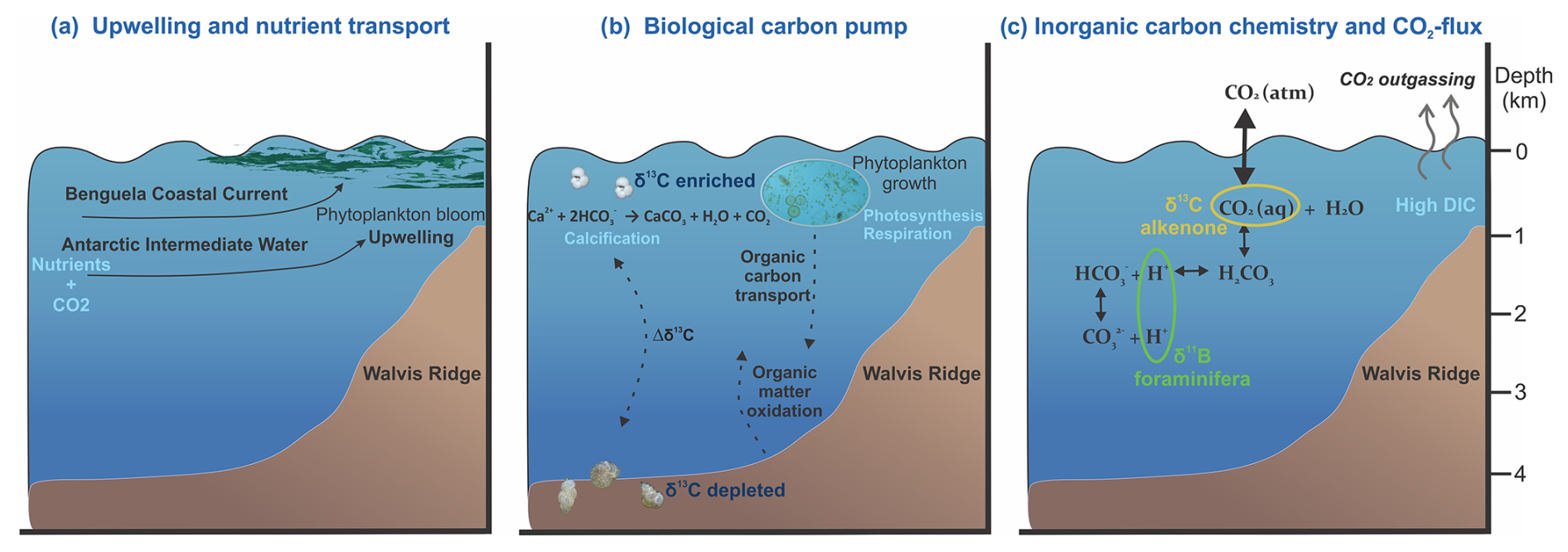
Figure 1 Cross-sections of the Benguela Upwelling System depicting the characteristics of an upwelling region, where (a) nutrient- and CO₂-rich waters are upwelled to the surface, (b) high productivity contributes to the drawdown of CO₂ in the surface layers via the biological carbon pump, and (c) the upwelling strength and efficiency of the biological carbon pump determine variations in the marine inorganic carbon chemistry and hence CO₂ flux.

The efficiency of the BCP determines how much of the newly produced particulate organic carbon at the surface is transported to the deep (Volk and Hoffert, 1985; Hain et al., 2014). During primary production, nutrients are consumed (e.g., nitrate, phosphate; Redfield, 1958) from the surface ocean and dissolved inorganic carbon (DIC) is taken up in organic matter, which is also reflected by the enrichment in ¹³C of the surface DIC (Degens et al., 1968). This implies that we can use seawater carbon isotopes as a proxy for the efficiency of the BCP. Seawater carbon isotopes can be reconstructed using the carbon isotopic composition (δ¹³C) in shells of carbonate producers, such as foraminifera. During high-productivity periods, the enhanced carbon uptake at the sea surface will enrich the shells of planktonic foraminifera in ¹³C. At the same time, the ¹³C-depleted carbon transported to the deep as organic matter will decrease the ¹³C content of the deep-water DIC pool, resulting in low δ¹³C values in the benthic foraminifera shells (Fig. 1b). Therefore, the stable carbon isotopic composition of these inorganic archives is imprinted by complex processes related to both surface to deep gradients and ocean circulations. Water masses of different origins carry distinct δ¹³C compositions resulting in integrated signatures of air–sea exchange and production/remineralization related to different water masses within the foraminiferal shells. The difference between planktonic and benthic δ¹³C, however, also records a measure for the efficiency of the BCP, where more divergent values between the surface and the deep indicate a more efficient BCP (Hilting et al., 2008).

This study focuses on the Benguela Upwelling System (BUS), as it is one of the major upwelling regions, where the strength of the upwelling and productivity changed over glacial–interglacial timescales. Whether upwelling intensity was stronger during glacial periods (Oberhänsli, 1991; Little et al., 1997; Kirst et al., 1999; Mollenhauer et al., 2003) or interglacial periods (Diester-Haass et al., 1992; Des Combes and Abelmann, 2007) is, however, still debated. Inconsistencies in the published body of work are possibly caused by seasonal differences between proxy signal carriers and/or major spatial- (depth-) related gradients, which is especially true for regions with strong CO₂ flux dynamics (Fig. 1c). Exchange of CO₂ between seawater and the atmosphere at these regions may be constrained only by applying multiple proxies that comprise various living depths and seasonal preferences. Therefore, here, we compare organic and inorganic proxies for temperature (U${}_{\mathrm{37}}^{K^{\prime }}$, Mg $/$ Ca) and the carbon system (alkenone δ¹³C, foraminiferal δ¹¹B) with reconstructed efficiency of the BCP in the Benguela upwelling area to unravel the potential role of such areas in known changes in atmospheric pCO₂ on glacial–interglacial timescales. At the same time, this allows us to compare proxies and investigate (in)consistencies between different carbon system and temperature proxies.

2 Oceanographic setting

The BUS is one of the four major eastern boundary upwelling systems, and it is located between 15 and 34° S along the coastline of Africa (Hill, 1998; Hart and Currie, 1960). This region bears the highest productivity today among the eastern boundary upwelling systems, fueled by nutrients transported mainly from the higher latitudes. Advection of the cold and nutrient-rich water is a persistent phenomenon throughout the year (Carr, 2001; Chavez and Messié, 2009), and the magnitude of the particulate organic carbon (POC) flux from the surface to the deep exceeds 20 gC m⁻² yr⁻¹ (Henson et al., 2011; Laws et al., 2000; DeVries and Weber, 2017).

The BUS is associated with the South Atlantic anticyclonic gyre, which gives rise to upwelling on its southeastern flank where it meets the African continent (Peterson and Stramma, 1991). The low-pressure system over western South Africa causes a pressure gradient between the continent and the ocean and thereby strengthens the southerly wind stress off the coast of Angola and Namibia. The interplay between the equatorward trade winds, the Coriolis force, and the presence of the continental boundary leads to the offshore transport of surface waters. As such, this causes coastal upwelling of nutrient-rich South Atlantic Central Water (formed in the western South Atlantic; Stramma and England, 1999) and Antarctic Intermediate Water (AAIW). The upwelled waters are transported equatorward along the coast of Africa via the Benguela Current (BC), giving rise to high biological productivity. Filaments of productive waters can be seen extending from the African continent (Fig. 2). Finally, the Walvis Ridge potentially plays a role in affecting local hydrography and hence the position of the upwelling (Peterson and Stramma, 1991).

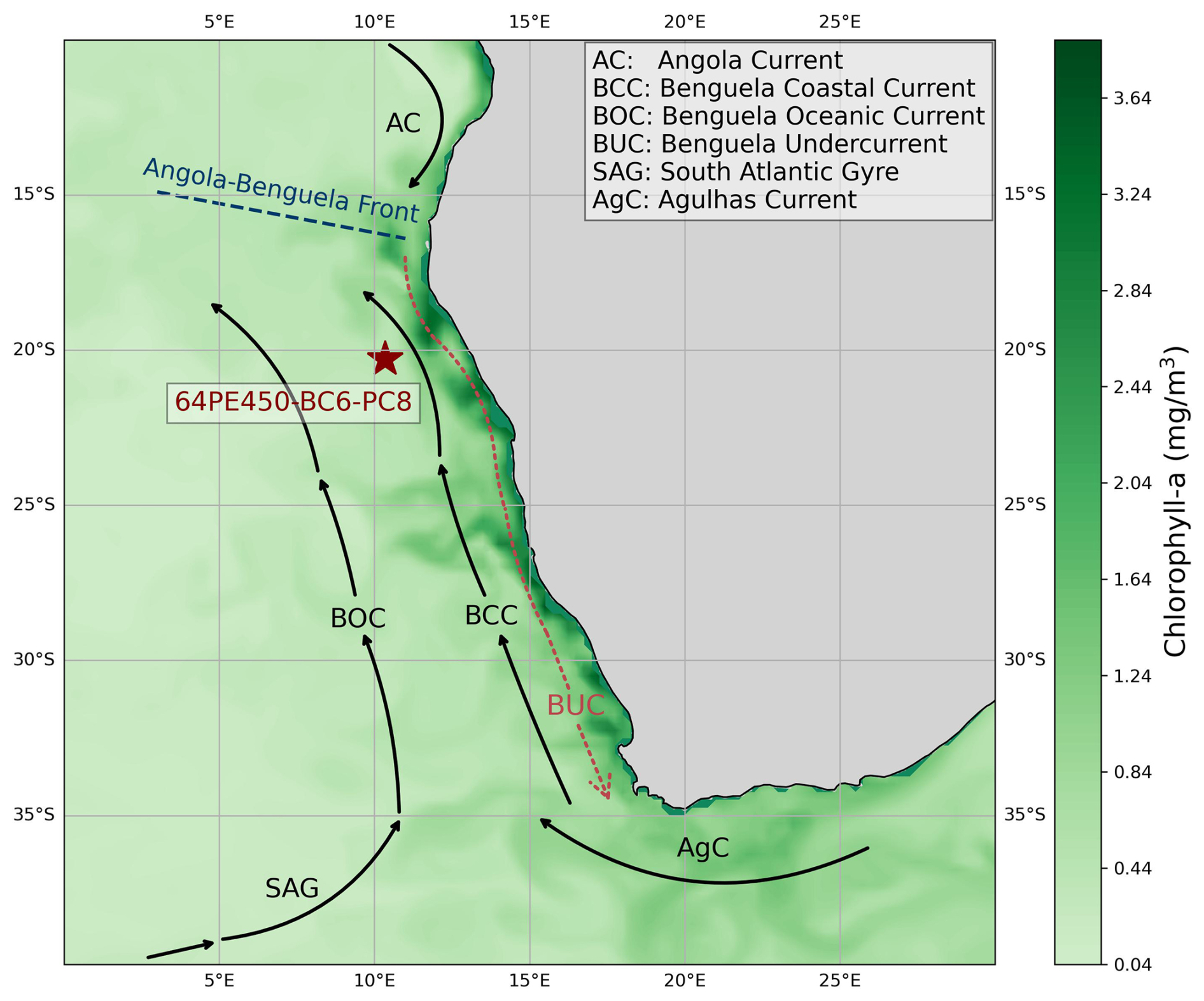
Figure 2 Map showing the location of sediment core 64PE450-BC6-PC8 and the dominant currents shaping the characteristics of the Benguela Upwelling System. The map is overlain with the distribution of surface water chlorophyll-a concentration of July 2023 obtained from Global Ocean Biogeochemistry Analysis and Forecast (EU Copernicus Marine Service information; https://doi.org/10.48670/moi-00015, Global Ocean Biogeochemistry Analysis and Forecast, 2024). High chlorophyll-a concentrations indicate the high productivity and nutrient-rich upwelled waters of this region today.

The BC, with its two main branches, the Benguela Oceanic Current and the Benguela Coastal Current, is the major northward-flowing component of the BUS which joins the poleward-flowing Angola Current in the north (Stramma and England, 1999). This convergence zone is located between 15 and 18° S and is known as the Angola–Benguela frontal zone. The upwelling zone is bounded by warm current systems, the Angola Current system in the north and the Agulhas Current system in the south (Shannon and Nelson, 1996; Shillington, 1998; Shannon and O'Toole, 2003). Hence, the BC is composed of a mixture of waters originating not only from the mid-latitude surface waters of the central South Atlantic Ocean and the Southern Ocean but also from the Indian Ocean (Gordon, 1986; Lutjeharms and Valentine, 1987). This creates a north-to-south decrease in surface water temperature and salinity in the region (Santana-Casiano et al., 2009). Hydrographic changes in the region over glacial cycles have been related to changes in the transfer of Indian Ocean waters through Agulhas leakage variability (Knorr and Lohmann, 2003; Peeters et al., 2004; Scussolini and Peeters, 2013).

The BUS region is characterized by year-round upwelling of varying intensity due to the seasonal shift in the South Atlantic gyre. This results in stronger upwelling intensities in June–August compared to the rest of the year (Santana-Casiano et al., 2009; Kämpf and Chapman, 2016). The spatial and temporal dynamics of the BUS result in large variability in the associated CO₂ flux. Predominantly, the surface waters within the BUS act as a CO₂ source (Laruelle et al., 2014; Brady et al., 2019; Roobaert et al., 2019), but this may be interrupted by periods during which they act as a CO₂ sink due to the high primary productivity (Gruber et al., 2009; Gregor and Monteiro, 2013).

3 Proxy interpretation

Reconstruction of inorganic carbon chemistry can be used to constrain past changes in the CO₂ flux between the ocean and atmosphere. Reconstruction of the complete inorganic carbon system is based on at least two parameters of this system (pCO₂, [CO${}_{\mathrm{3}}^{\mathrm{2}-}$], [HCO${}_{\mathrm{3}}^{-}$], pH, [DIC], and total alkalinity) and on the knowledge of temperature and salinity (Zeebe and Wolf-Gladrow, 2001). Commonly used tracers for constraining parameters of the marine inorganic carbon chemistry are based on both organic (e.g., δ¹³C of alkenones; Pagani et al., 2002; Pagani, 2014; Popp et al., 1998; Laws et al., 1995) and inorganic (e.g., δ¹¹B of foraminifera shells; Hemming and Hanson, 1992; Palmer and Pearson, 2003; Foster and Rae, 2016) proxy signal carriers, although these proxies rarely agree completely for upwelling regions (Seki et al., 2010; Palmer et al., 2010) or in general (Rae et al., 2021).

Proxies for seawater carbon chemistry have specific inherent complications, and their application requires critical assumptions. For instance, previous studies have observed discrepancies between alkenone-based pCO₂ reconstruction and ice core records (Palmer et al., 2010; Andersen et al., 1999; Zhang et al., 2013; Witkowski et al., 2020; Jasper et al., 1994), which could be related to disequilibrium between the sea surface and the atmosphere, especially at dynamic sites like upwelling regions. However, it may also be explained by the process of CO₂ uptake in the algal cell, if passive diffusion is not the only way alkenone producers acquire CO₂ in the cell, as suggested by the traditional framework of this proxy (Bidigare et al., 1997). Alkenone producers do use a carbon-concentrating mechanism (CCM; Stoll et al., 2019; Reinfelder, 2011; Bolton and Stoll, 2013; Badger, 2021), which enables carbon acquisition in the cell through the active pumping of HCO${}_{\mathrm{3}}^{-}$ to the chloroplast during low pCO₂ conditions. Also, pCO₂ reconstructions based on alkenone δ¹³C values are subject to uncertainties related to the so-called b factor that expresses the effect of multiple parameters related to the physiology of the alkenone producers (Jasper et al., 1994; Rau et al., 1996; Popp et al., 1998). Application of the b factor for the reconstruction of pCO₂ is much debated (e.g., Wilkes and Pearson, 2019), and an adaptation of CCM by the alkenone producers inevitably hampers the application of the proxy. However, there are examples of alkenone-based pCO₂ reconstructions reliably reproducing glacial–interglacial pCO₂ variability (Palmer et al., 2010; Jasper and Hayes, 1990; Bae et al., 2015), potentially related to specific local conditions. As the b value is best represented by a linear relationship to nutrient availability (Bidigare et al., 1997), we rely on the analysis of the barium-to-calcium ratio (Ba $/$ Ca) in planktonic foraminiferal shells that correlates with seawater Ba concentration; hence we used it as a proxy for seawater [PO${}_{\mathrm{4}}^{\mathrm{3}-}$] (Lea and Boyle, 1989; Lea and Boyle, 1990b, a; Hönisch et al., 2011).

4 Materials and methods

Samples were taken from box core 64PE450-BC6 and piston core 64PE450-PC8 retrieved from the southern flank of the Walvis Ridge, both taken at the same location (approximately 20.29° S, 10.35° E) at a water depth of ∼ 1375 m b.s.f. The box core consisted of 40.59 cm of sediment, whereas the piston core collected 1453 cm (cut into 15 sections, of which we dated the first 100 cm). The top of the piston core was missing; hence, we used the BC to supplement the missing top of the PC and obtain a near-continuous record, which we here refer to as 64PE450-BC6-PC8. To align the box core and the piston core, lightness reflectance data (L*) were used here as an additional constraint to the radiocarbon dates (Supplement Fig. S1). The detailed reflectance data (63 µm resolution) show an overlap between the two cores. The top 4.24 cm of 64PE450-PC8 (later referred to as the disturbed core-top) overlaps with approximately 30.14 cm of 64PE450-BC6 (i.e., from 10.45 to 40.59 cm b.s.f.). This suggests severe compression of the top of 64PE450-PC8, likely due to the piston coring, but the overlap can still be used to align the age model of the two cores.

The composite record was sampled with a resolution varying between 2 and 5 cm to optimize coverage of the glacial–interglacial transition. All samples were freeze-dried and subsequently split into sub-samples to obtain lipid biomarkers and foraminifera from the same core depth.

4.1 Foraminiferal sample cleaning

Due to their relatively high abundance in upwelling regions and common use in paleoclimate reconstructions (e.g., Spero and Lea, 1996), we selected specimens of Globigerina bulloides for the planktonic-foraminifera-based records. Freeze-dried samples were washed over a 63 µm sieve, dried, and further dry-sieved to separate size fractions of 150–315 and 315–425 µm. Specimens of G. bulloides were picked from the latter size fraction for analysis of oxygen and carbon isotopes, minimizing any potential impacts of ontogeny. However, as many more specimens were needed, the smaller size fraction was used for radiocarbon, element $/$ calcium (El $/$ Ca), and boron isotope analysis. The foraminifer's size has been shown to affect boron isotopes of several symbiont-bearing planktonic foraminifera species (e.g., T. sacculifer, G. ruber, O. universa; Hönisch and Hemming, 2004; Henehan et al., 2013; Henehan et al., 2016); hence size fraction need to be minimized to avoid introducing uncertainties related to ontogenetic variability. G. bulloides is a symbiont-barren species; therefore, boron isotopes are not affected by pH change in their microenvironments related to the symbionts' physiological processes (i.e., respiration, photosynthesis). However, differences in shell size may correspond to different environmental conditions and, for instance, reflect changes in calcification depth and/or seasons (Jonkers et al., 2013; Osborne et al., 2016). Also, previous studies using G. bulloides to reconstruct pH relied on a narrow size fraction when the number of specimens allowed this (Raitzsch et al., 2018; Martinez-Boti et al., 2015). Alternatively, a combination of two or more parameters (e.g., temperature and productivity) may impact shell size, resulting in mixed isotopic signatures within size fractions (Metcalfe et al., 2015). Any size-dependent bias on boron isotopes of (symbiont-barren) foraminifera still needs to be investigated; hence we assume that the data presented here for G. bulloides reflect average conditions with respect to depth and seasonal variability. To construct a benthic foraminiferal carbon isotope record, specimens of Cibicidoides wuellerstorfi were selected from the 315–425 µm size fraction.

Foraminiferal samples were cleaned prior to the analysis of El $/$ Ca ratios and stable isotopes, following an adapted protocol of Barker et al. (2003). This adapted protocol is as follows: for the analysis of the shells' element concentrations in solution and the boron isotopic composition, specimens were carefully cracked using a scalpel to open up the chambers and release potential clay content from the inside. The samples were subsequently transferred to acid-cleaned 1.5 mL vials (Treff) and rinsed three times with deionized water (Milli-Q) and twice with methanol, followed by another thorough rinse with deionized water, using ultrasonication for each rinsing step. To remove all organic material from the shells, samples were placed in a hot block and oxidized with NH₄OH-buffered 1 % H₂O₂ solution for 45 min at 90 °C. To ensure complete removal of organic material, this step was repeated up to three times based on visual inspection. After the oxidative cleaning, the samples were transferred to new pre-cleaned vials (Treff) and leached with diluted acid (1 mM HNO₃) followed by rinsing the samples three times with deionized water. Because the boron isotope analysis is very sensitive to contamination, two additional leaching steps with 1 % NH₄OH were added, followed by rinsing with deionized water, before the acid leaching. Samples for El $/$ Ca and δ¹¹B analysis were finally dissolved in 500 µL 0.1 M ultra-grade HNO₃ and in 75–80 µL 0.5 M ultra-grade HNO₃, respectively.

Specimens taken for the analysis of El $/$ Ca ratios with a laser ablation quadrupole inductively coupled plasma mass spectrometer (LA-Q-ICP-MS) and for the measurement of δ¹⁸O and δ¹³C were cleaned following the same clay removal and oxidative cleaning step as described above but without cracking the shells before the cleaning steps.

4.2 Radiocarbon analysis

Radiocarbon analysis (¹⁴C/¹²C) on 50–100 specimens of well-preserved shells of G. bulloides was performed at the Laboratory of Ion Beam Physics, ETH Zürich. The analysis of ¹⁴C/¹²C followed the protocol described in Wacker et al. (2013, 2014). Briefly, samples were measured with a gas ion source in a Mini Carbon Dating System (MICADAS; Synal et al., 2007) with an automated method for acid digestion of carbonates (Wacker et al., 2013). Samples were placed in 4.5 mL exetainer vials (Labco Limited^®, UK) and purged with a flow of 60 mL min⁻¹ of helium for 10 min and subsequently leached with 100 µL 0.02 M ultrapure HCl with an automated syringe to remove adsorbed contaminants. Analysis of the released CO₂ from both the leachate and remaining sample provided confirmation for the near-complete removal of contaminants. The CO₂ released from the leachate was directly transported by helium to a zeolite trap and injected into the ion source for ¹⁴C/¹²C analysis. The remaining leached sample was acidified with 100 µL ultrapure H₃PO₄ (85 %) and heated at 60 °C for a minimum of 1 h. The released CO₂ was then injected into the ion source for analysis (Wacker et al., 2014; Fahrni et al., 2013). The difference between the radiocarbon values of the leachate and leached samples was less than 5 %. Radiocarbon determinations are given in the conventional radiocarbon ages and corrected for isotopic fractionation via ¹³C $/$ ¹²C isotope ratios. Calibration was performed using the Marine20 calibration curve (Heaton et al., 2020) with a local correction to the marine reservoir age (ΔR) of 146 ± 85 ¹⁴C years (Dewar et al., 2012). These calculations were computed using the Bayesian age–depth model in the Bacon v2.3 package for the R statistical programming software (Blaauw and Christen, 2011).

4.3 Analysis of stable oxygen and carbon isotopes

Pre-weighed 20–40 µg of the shells of G. bulloides were dissolved in orthophosphoric acid and analyzed at 71 °C by a Kiel IV device coupled to a MAT 253 isotope-ratio mass spectrometer (IRMS; Thermo Fisher Scientific^®) at the NIOZ. Analyses were calibrated using standard bracketing (NBS-19), and the NIOZ house standard (NFHS-1; Mezger et al., 2016) was used to monitor drift. Accuracy and precision for δ¹³C = 0.814 ± 0.04 ‰ and δ¹⁸O = 1.024 ± 0.12 ‰ were calculated across several analytical runs of NFHS-1 (±1σ SD, n=64).

4.4 Analysis of foraminiferal element $/$ calcium ratios

Prior to the analysis of the samples in solution, a few planktonic foraminifera specimens were screened for preservation to minimize the possibility of diagenetic overprint affecting the geochemical signature of the shells. For this, the ratios of ²³Na $/$ ⁴³Ca, ²⁴Mg $/$ ⁴³Ca, ²⁵Mg $/$ ⁴³Ca, ²⁷Al $/$ ⁴³Ca, ⁵⁵Mn $/$ ⁴³Ca, and ⁸⁸Sr $/$ ⁴³Ca were simultaneously monitored during the ablation of single chambers of G. bulloides by a laser ablation quadrupole inductively coupled plasma mass spectrometer (LA-Q-ICP-MS). Laser ablation data were acquired on 60 µm diameter spots with a repetition rate of 4 Hz and a laser energy density of ∼ 1 J cm⁻². The JCp (Porites sp. coral) nano-pellet was used to monitor instrumental drift, and JCt (Tridacna gigas giant clam; Okai et al., 2004), MACS-3, and the NIOZ Foraminifera House Standard-2-Nano-Pellet (NFHS-2-NP; Boer et al., 2022) provided further quality control on the measurement. NIST SRM 610 was used as the calibration standard. Data were evaluated as both profiles and shell averages.

Approximately 40–50 specimens of G. bulloides were dissolved for solution analyses using a sector field inductively coupled plasma mass spectrometer (SF-ICP-MS; Thermo Fisher Scientific^® Element 2). The applied cleaning procedure is based on Barker et al. (2003), as discussed above. A pre-scan of calcium concentrations ([Ca²⁺]) was performed on an aliquot of 30 µL of the dissolved samples, and, based on those data, all samples were subsequently diluted to match [Ca²⁺] (100 ppm) for element analyses. Isotopes of ²⁵Mg and ¹³⁸Ba were measured in low resolution. All samples were measured against four ratio calibration standards (de Villiers et al., 2002) and alternated with 0.1 M HNO₃ in between samples to increase the efficiency of wash-out. All samples are drift-corrected using the NFHS-1 standard (Mezger et al., 2016) and three additional standards, NFHS-2 (Boer et al., 2022), JCp, and JCt (Okai et al., 2004), to evaluate accuracy and precision of the analytical runs. Uncertainty from the internal precision on the basis of short-term stability is <2 % for both Mg, and Ba. Samples were analyzed in replicates yielding an uncertainty of <0.02 mmol mol⁻¹ for Mg and <0.14 µmol mol⁻¹ for Ba.

4.5 Micro-distillation and boron isotope analysis

Approximately 150 specimens of G. bulloides were cleaned for the analysis of boron isotopes. Boron was separated from the calcium carbonate matrix via the micro-distillation technique (Gaillardet et al., 2001; Wang et al., 2010; Misra et al., 2014). A total of 70 µL of the sample was placed on the lid of a Teflon^® fin-legged conical beaker (5 mL) and placed upside down on a hotplate at 100 °C for 20–24 h. The fin-legged vials were wrapped in aluminum foil to provide a heat gradient for a more efficient separation of boron. Once the micro-distillation was complete, the vials were carefully removed from the hotplate while being turned over and were subsequently left for cooling. Sample residue was removed by putting new lids on the beakers, and each sample was diluted with 0.2 M HF +0.2 M HNO₃ for a pre-scan of the boron concentration ([B]). Based on the results of the pre-scan, a final dilution was made to set [B] at 5 ppb for the analysis of δ¹¹B.

Analysis of the micro-distilled samples was performed at the NIOZ on a Neptune Plus multi-collector inductively coupled plasma mass spectrometer (MC-ICP-MS; Thermo Fisher Scientific^®) equipped with high-performance extraction cones (Jet sample cone and “X” skimmer cone) to maximize sensitivity for boron. Samples were injected using a Savillex^® 50 µL min⁻¹ C-flow nebulizer and Teflon^® Scott-type spray chamber. Beams of ¹⁰B and ¹¹B were measured on L3 and H3 Faraday cups equipped with amplifiers using 10¹³Ω resistors (Misra et al., 2014; Lloyd et al., 2018). The instrument was tuned to obtain a stable sensitivity, typically 15–25 mV ppb⁻¹ B.

Solutions of 0.2 M HF + 0.2 M HNO₃ were used for rinsing throughout the analytical run between analyses and as a matrix for each sample and standard. The analysis followed the approach of sample–standard bracketing using NIST 951 as a reference standard. All samples and quality control standards were analyzed in duplicates; thus average values with ±2σ standard deviations are reported here. Samples with a replicate precision higher than ± 0.6 ‰ (2σ) were excluded from this study. A coral standard (Chanakya and Misra, 2022) was treated with the complete carbonate cleaning and micro-distillation procedure for each analytical sequence and repeatedly analyzed to monitor long-term precision (δ¹¹B = 24.57 ± 0.65 ‰ 2σ, n=64). Additionally, non-micro-distilled AE-121 standard was analyzed within each run for quality control (δ¹¹B = 19.48 ± 0.33 ‰ 2σ, n=46).

In addition to the coral standard, the initial test analysis to validate the boron purification method and instrumental accuracy and precision also included repeated measurements of seawater (Southern Ocean, δ¹¹B = 39.72 ± 0.25 ‰ 2σ, n=5) and a boron standard (AE-121) mixed with CaCO₃ (trace metal basis, Acros Organics^® ) to mimic foraminiferal calcium concentrations (δ¹¹B = 19.53 ± 0.25 ‰ 2σ, n=18).

4.6 Estimating past salinity and foraminifera-based temperatures, pH, and pCO₂

Sea surface temperatures (SSTs) were calculated from foraminiferal Mg $/$ Ca values using the species-specific temperature calibration of Mashiotta et al. (1999),

$$\begin{array}{}\text{(1)}& \mathrm{Mg}/\mathrm{Ca}=\mathrm{0.47}(\pm \mathrm{0.03})\times e^{\mathrm{0.107}(\pm \mathrm{0.003})\times \mathrm{SST}},\end{array}$$

where propagated error was calculated based on 1 standard deviation of the duplicate analysis of Mg $/$ Ca and the uncertainty derived from the calibration equation. Mg $/$ Ca values of planktonic foraminifera are known to be affected by salinity and pH changes as well (Gray et al., 2018; Dueñas-Bohórquez et al., 2009; Gray and Evans, 2019); however, a correction for these effects requires independent estimates for salinity and pH with species-specific calibrations. For calculating past carbon chemistry, salinity is an important parameter, and it was estimated based on its conservative relationship with relative sea level change (Waelbroeck et al., 2002). Modern seawater salinity of the BUS (35.43 ± 0.30) was derived from the WOCE Global Data Version 3.0 (Schlitzer, 2000) based on the five closest data points to the location of core 64PE450-BC6-PC8. Using these salinity estimates, the effect of salinity on Mg $/$ Ca-based SST was evaluated and found to have only a small offset in SST values (<0.4 °C). As the effect of salinity is relatively minor and adding it would also introduce additional uncertainties, we decided here to refrain from correcting for salinity and pH when calculating past temperatures.

The measured δ¹¹B values of G. bulloides were converted into pH (Hemming and Hanson, 1992) using Eq. (2):

$$\begin{array}{}\text{(2)}& \begin{array}{rl}\mathrm{pH}=p{K}_B^{\ast }& -\log (-({\mathit{\delta }}^{\mathrm{11}}{B}_{\mathrm{sw}}-{\mathit{\delta }}^{\mathrm{11}}{B}_{\mathrm{borate}})/\\ & ({\mathit{\delta }}^{\mathrm{11}}{B}_{\mathrm{sw}}-\mathit{\alpha }\times {\mathit{\delta }}^{\mathrm{11}}{B}_{\mathrm{borate}}-\mathit{\epsilon })),\end{array}\end{array}$$

where the equilibrium constant, $p{K}_B^{\ast }$ (Dickson, 1990), was calculated for each sample based on SST derived from the Mg $/$ Ca values of G. bulloides and salinity based on sea level. The fractionation factor between B(OH)₃ and B(OH)${}_{\mathrm{4}}^{-}$, expressed here as α, is 1.0272 ± 0.0006, from which fractionation, ε, is derived as 27.2 ± 0.6 (Klochko et al., 2006). The boron isotopic composition of seawater, δ¹¹B_sw, is 39.61 ± 0.2 ‰, based on a large range of temperature, salinity, and depth conditions (Foster et al., 2010), and the δ¹¹B of borate was calculated from the measured δ¹¹B of G. bulloides using the species-specific core-top calibration from Raitzsch et al. (2018).

Constraining pCO₂ based on seawater pH requires knowledge of a second independent parameter (Zeebe and Wolf-Gladrow, 2001). For this purpose, total alkalinity was assumed to be the same as today's value at the BUS. Taking the five nearest available data points at the core location from the GLODAPv2023 dataset (Lauvset et al., 2024) defines an average value of 2349 ± 11 µmol kg⁻¹, which was used to supplement the pH-based pCO₂ reconstruction throughout the 27 kyr record.

Uncertainty on the reconstructed pH value was determined for each sample through error propagation that considered the abovementioned uncertainties of $p{K}_B^{\ast }$, α, ε, and δ¹¹B_sw and the standard deviation (external uncertainty) based on duplicate or triplicate analysis of foraminiferal δ¹¹B.

Concentrations of CO₂ are based on pH and inorganic carbon chemistry calculations using the PyCO2SYS package (Humphreys et al., 2022) in Python version 3.11.2. Uncertainty is propagated for each computed carbon chemistry parameter as described in Humphreys et al. (2022).

4.7 Lipid extraction and alkenone analyses

Lipids were extracted from the freeze-dried and homogenized sediment samples using an accelerated solvent extractor (ASE^® 350, DIONEX^®) at the NIOZ. Samples were extracted with dichloromethane (DCM) and methanol (9:1, $v/v$) at 100 °C to obtain the total lipid content and subsequently dried under N₂ gas at 35 °C in a Caliper TurboVap LV Evaporator. Samples were then redissolved in DCM and run through an Na₂SO₄ column to eliminate excess water. The extract was passed through an alumina (Al₂O₃) column and separated into apolar, ketone, and polar fractions using a mixture of hexane : DCM (9:1, $v/v$), hexane : DCM (1:1, $v/v$), and DCM : methanol (1:1, $v/v$), respectively. All extracts were dried under N₂, and the ketone fraction was further utilized to obtain the relative abundance and δ¹³C values of the long-chain alkenones.

Ketone fractions were dissolved in ethyl acetate, and concentrations of alkenones were measured using a gas chromatograph with flame ionization detection (GC-FID; Agilent^® 6890N) equipped with a silica capillary column (CP-Sil 5 CB; 50 m × 0.32 mm, 0.12 µm film thickness). The temperature program of the GC-FID analyses used an initial temperature of 70 °C that increased with a rate of 20 °C min⁻¹ to 200 °C followed instantly by heating at a rate of 3 °C min⁻¹ until it reached 320 °C, where it remained constant for 10 min.

Based on the initial concentration measurement, samples were diluted with ethyl acetate to allow stable carbon isotope analysis using a gas chromatography isotope ratio mass spectrometer (GC-IRMS; Thermo Fisher Scientific^® Delta V Advantage Trace^® 1310). The GC-IRMS was equipped with cross-bond trifluoropropylmethyl polysiloxane columns (Rtx-200; 60 m × 0.32 mm, 0.5 µm film thickness) and helium as a carrier gas. Each sample was manually injected onto the GC-IRMS. The starting temperature of the GC-IRMS was 70 °C, which then increased by 18 °C min⁻¹ until reaching 250 °C. After reaching that temperature, heating continued with 1.5 °C min⁻¹ until 320 °C, where it was kept stable for 25 min. Samples were analyzed for carbon isotopes in duplicates, and instrumental accuracy was monitored through measurement of the B5 n-alkane mixture standard (provided by A. Schimmelmann, Indiana University) every day (i.e., after every 6–7 samples). The IsoLink II combustion reactor was oxidized for 10 min every day before the start of standard and sample analysis. Each analysis was followed by 2 min of seed oxidation to maintain the reactor oxygenation.

4.8 Calculation of alkenone-based temperatures and pCO₂

Alkenone-based sea surface temperatures were derived from the ketone unsaturation index (U${}_{\mathrm{37}}^{K^{\prime }}$), where U${}_{\mathrm{37}}^{K^{\prime }}$ is defined as the relative abundance of di- and tri-unsaturated C₃₇ methyl alkenones (Prahl and Wakeham, 1987):

$$\begin{array}{}\text{(3)}& {\mathrm{U}}_{\mathrm{37}}^{K^{\prime }}={\mathrm{C}}_{\mathrm{37}:\mathrm{2}}/({\mathrm{C}}_{\mathrm{37}:\mathrm{3}}+{\mathrm{C}}_{\mathrm{37}:\mathrm{2}}).\end{array}$$

Sea surface temperature was then calculated using the alkenone temperature calibration model developed for the Atlantic region (Conte et al., 2006).

Fractionation of stable carbon isotopes during photosynthesis (ε_p37:2) can be computed based on the difference between the carbon isotopic ratio of aqueous carbon dioxide (δ¹³C${}_{{\mathrm{CO}}_{\mathrm{2}}}$) and the organic biomass (δ¹³C_org):

$$\begin{array}{}\text{(4)}& {\mathit{\epsilon }}_{p\mathrm{37}:\mathrm{2}}=\left[\right({\mathit{\delta }}^{\mathrm{13}}{\mathrm{C}}_{{\mathrm{CO}}_{\mathrm{2}}}+\mathrm{1000})/({\mathit{\delta }}^{\mathrm{13}}{\mathrm{C}}_{\mathrm{org}}+\mathrm{1000})-\mathrm{1}]\times \mathrm{1000}.\end{array}$$

δ¹³C${}_{{\mathrm{CO}}_{\mathrm{2}}}$ was derived from the carbon isotopes of planktonic foraminifera, G. bulloides, corrected for the temperature-dependent fractionation during calcite precipitation (Romanek et al., 1992) and the fractionation between dissolved and gaseous carbon dioxide (Mook et al., 1974).

δ¹³C_org was calculated from the carbon isotopes of di-unsaturated alkenones (δ¹³C_37:2) as

$$\begin{array}{}\text{(5)}& {\mathit{\delta }}^{\mathrm{13}}{\mathrm{C}}_{\mathrm{org}}=\left[\right({\mathit{\delta }}^{\mathrm{13}}{\mathrm{C}}_{\mathrm{37}:\mathrm{2}}+\mathrm{1000})\times (\mathrm{\Delta }{\mathit{\delta }}^{\mathrm{13}}{\mathrm{C}}_{\mathrm{org}}+\mathrm{1}\left)\right]-\mathrm{1000},\end{array}$$

where Δδ¹³C_org expresses the carbon isotopic difference between C_37:2 and DIC, which has been defined between 3 ‰–6 ‰ based on culture experiments (Riebesell et al., 2000; Schouten et al., 1998; van Dongen et al., 2002). Here, we take the commonly applied value of 4.2 ‰ (Bijl et al., 2010; Pagani et al., 2005; Pagani et al., 2010; Pagani et al., 2011; Seki et al., 2010; Palmer et al., 2010).

Based on ε_p37:2, aqueous CO₂ ([CO₂]_aq) can be reconstructed as follows (Hayes, 1993; Pagani et al., 2002):

$$\begin{array}{}\text{(6)}& [{\mathrm{CO}}_{\mathrm{2}}{]}_{\mathrm{aq}}=b/({\mathit{\epsilon }}_{\mathrm{f}}-{\mathit{\epsilon }}_{p\mathrm{37}:\mathrm{2}}),\end{array}$$

where ε_f stands for the carbon isotopic fractionation associated with carbon fixation estimated as 25 ‰ (e.g., Popp et al., 1998). Parameter b expresses all physiological factors affecting total carbon isotope fractionation, including cell shape and size, membrane permeability, and the algae's growth rate (Jasper et al., 1994; Rau et al., 1996; Popp et al., 1998; Conte et al., 1994; Riebesell et al., 2000). Earlier studies using phytane (Bice et al., 2006; Damsté et al., 2008) and alkenone (Witkowski et al., 2018) to reconstruct pCO₂ estimated b for a mean value of 165 ‰–170 ‰ kg µM⁻¹. As growth rate and thereby nutrient availability have a large influence on the physiological factors and, accordingly, b values are highly correlated to [PO${}_{\mathrm{4}}^{\mathrm{3}-}$] (Bidigare et al., 1997), b can be best described at our core site by estimating past changes in [PO${}_{\mathrm{4}}^{\mathrm{3}-}$] (Pagani et al., 2005). Here, [PO${}_{\mathrm{4}}^{\mathrm{3}-}$] is estimated based on the Ba $/$ Ca ratio of planktonic foraminifera, G. bulloides (Lea and Boyle, 1989; Lea and Boyle, 1990b, a; Martin and Lea, 1998; Lea and Boyle, 1991). We therefore constrain past changes in b as (Pagani et al., 2005)

$$\begin{array}{}\text{(7)}& \begin{array}{rl}b& =[\mathrm{118.52}\times (\mathrm{Ba}/\mathrm{Ca}\times [{\mathrm{PO}}_{\mathrm{4}}^{\mathrm{3}-}{]}_{\mathrm{modern}}/{\mathrm{Ba}/\mathrm{Ca}}_{\mathrm{modern}})\\ & +\mathrm{84.07}].\end{array}\end{array}$$

Average modern PO${}_{\mathrm{4}}^{\mathrm{3}-}$ concentration ([PO${}_{\mathrm{4}}^{\mathrm{3}-}$]_modern) in the BUS is 0.63 µmol kg⁻¹ (obtained from GLODAPv2023; Lauvset et al., 2024; Olsen et al., 2016; Key et al., 2015), whereas the corresponding modern foraminiferal Ba $/$ Ca value (Ba $/$ Ca_modern) was analyzed here (19.08 µmol mol⁻¹). Equation (7) basically assumes a constant and proportional relation between Ba and [PO${}_{\mathrm{4}}^{\mathrm{3}-}$]. This seems reasonable for our purposes, as surface water Ba concentration has been shown to be reflected proportionally in foraminiferal Ba $/$ Ca (Lea and Boyle, 1991; Hönisch et al., 2011) and the cold nutrient-rich surface waters are generally enriched in dissolved barium (e.g., Davis et al., 2020).

To calculate atmospheric pCO₂ from aqueous concentrations of CO₂, Henry's law was applied using the temperature- and salinity-dependent solubility constant, K₀.

$$\begin{array}{}\text{(8)}& p{\mathrm{CO}}_{\mathrm{2}}=[{\mathrm{CO}}_{\mathrm{2}}{]}_{\mathrm{aq}}/K_{\mathrm{0}}\end{array}$$

Uncertainty propagation for the calculated pCO₂ values was based on the errors derived from 1 standard deviation of duplicate analysis of δ¹³C of the extracted ketone fraction, δ¹³C of foraminifera, and Ba $/$ Ca values of foraminifera. The largest uncertainty in alkenone-based pCO₂ reconstructions originates from the estimated past [PO${}_{\mathrm{4}}^{\mathrm{3}-}$], and, to incorporate potential variation in nutrient levels during the deglaciation, an additional uncertainty of 0.2 µmol kg⁻¹ was assigned to the known modern values of [PO${}_{\mathrm{4}}^{\mathrm{3}-}$]. This uncertainty is based on the gradient measured today in the upper 50 m of the water column, which is more than the variability observed in surface water today but also includes potential changes in the upwelled waters.

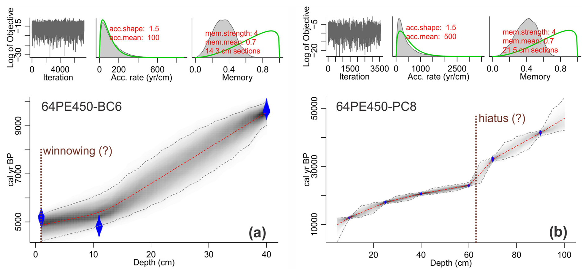
Figure 3 Age–depth model of (a) 64PE450-BC6 (box core) and (b) 64PE450-PC8 (piston core) based on radiocarbon dates, where blue diamonds indicate the sampling depth for ¹⁴C analysis. The calibration of radiocarbon ages and the figure was generated using the Bacon v2.3 package for the R statistical programming software (Blaauw and Christen, 2011). Calibration was performed using the Marine20 calibration curve (Heaton et al., 2020) with a local carbon reservoir correction (ΔR) of 146 ± 85 ¹⁴C years (Dewar et al., 2012). Dashed red lines show mean values of the best-fitted model, and dashed gray lines indicate the 95 % confidence interval. Note that, due to the disturbed core-top and potential hiatus in the piston core as indicated in panel (b), only the interval from 4.25 to 65.5 cm of 64PE450-PC8 was used for temperature and carbon system reconstruction in this study.

5 Results

5.1 Radiocarbon ages

The calibrated mean radiocarbon ages generally increase with depth in both BC and PC cores used here. Sediment core 64PE450-BC6 comprises 40.59 cm, where the core-top sample was dated at 4.863 ka, and an age of 9.551 ka at 40 cm b.s.f. (Fig. 3a). This suggests an average sedimentation rate of about 10 cm kyr⁻¹, with somewhat higher values (>10 cm kyr⁻¹) in the top 12 cm. Radiocarbon dates at the top of the box core (0–11 cm) indicate reversed ages (4.9 ka at 11 cm and 5.2 ka at 1 cm uncalibrated ages). This interval also corresponds to elevated Ca $/$ Al, Ti $/$ Al, and Si $/$ Al ratios measured through X-ray fluorescence (XRF) core scanning (Fig. S2; using the method described in Weltje and Tjallingii, 2008). The enrichment of elements commonly found in coarse fractions and heavy minerals is likely due to the removal of fine-fraction material by winnowing, which may have also contributed to the loss of the last 4.8 kyr in the sedimentary record. Alternatively, the upper 10 cm b.s.f. has constant ages due to bioturbation. Radiocarbon analyses from sediment core 64PE450-PC8 included six samples of the upper 100 cm of sediment collected. The age–depth model for this core suggests 9.994 ka at 5 cm b.s.f. depth (Fig. 3b) and indicates the presence of a disturbed core-top. Low sedimentation rates (2 cm kyr⁻¹) characterize the top 10 cm b.s.f. of this core, which is approximately in line with the sedimentation rate in the deepest parts of box core 64PE450-BC6 (∼ 6 cm kyr⁻¹). However, the average sedimentation rate in 64PE450-PC8 is lower (4 cm kyr⁻¹) compared to the average values observed in the box core, which, in part, might also be due to compaction with increasing depth. The top 60 cm b.s.f. of the core shows a steady increase in sedimentation rate (2–7 cm kyr⁻¹); therefore the low average values may be attributed to a relatively abrupt decrease in sedimentation rate at 60 cm b.s.f. in the core, which corresponds to an age of 23.586 ka. Between 60 and 100 cm b.s.f. depth, sedimentation rates remain 1–2 cm kyr⁻¹. Due to the uncertainty related to sediment deposition between 60 and 100 cm b.s.f. of the piston core, this study focuses only on the 40.59 cm b.s.f. of core 64PE450-BC6 and the upper 65.5 cm b.s.f. of core 64PE450-PC8.

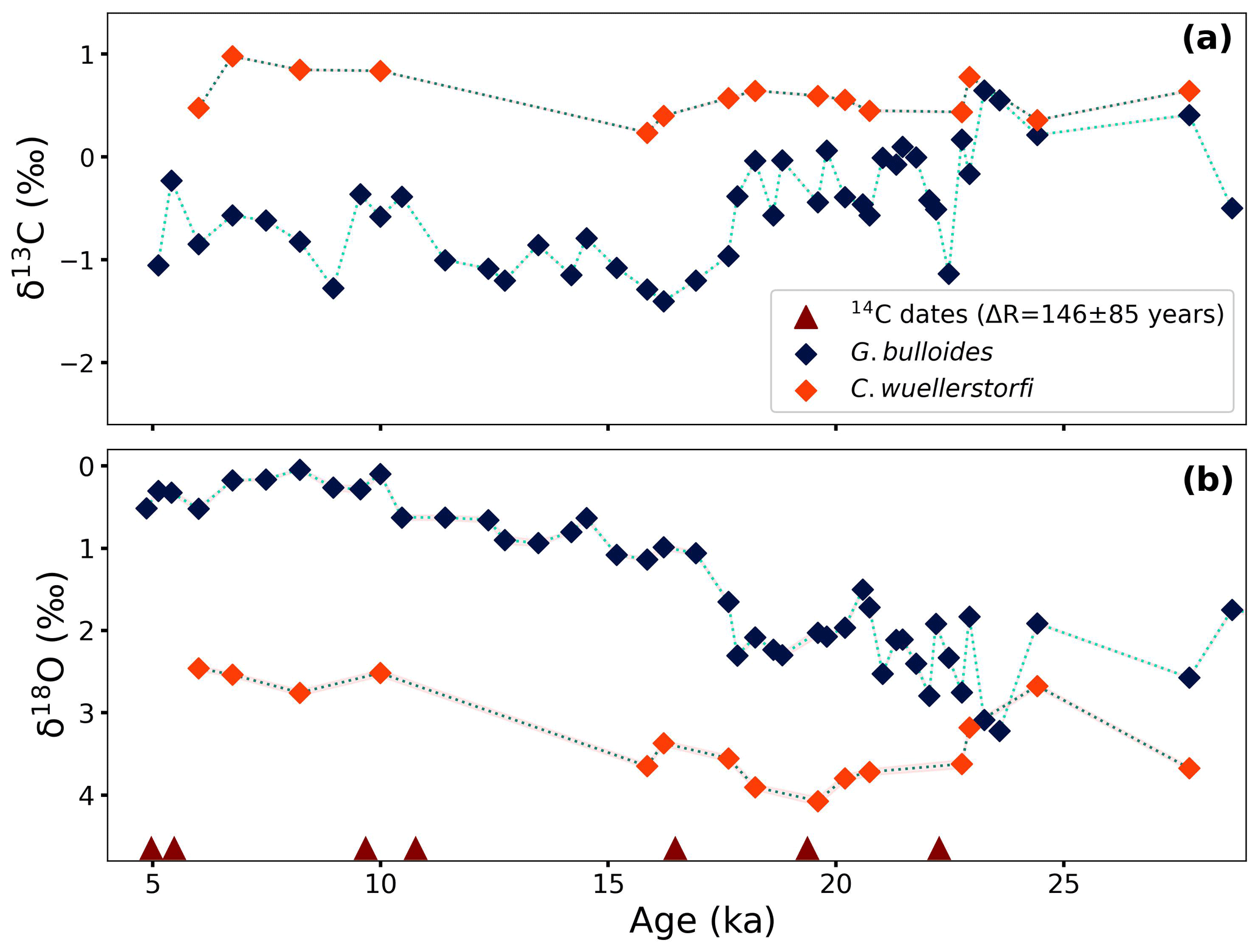
Figure 4 (a) δ¹³C and (b) δ¹⁸O values of planktonic (G. bulloides) and benthic (C. wuellerstorfi) foraminifera plotted with the age model. Red triangles indicate the ages tied with radiocarbon dates.

5.2 Stable isotopes

Carbon isotope values of the planktonic foraminifer, G. bulloides, vary between −1.4 ‰ and 0.6 ‰ (VPDB). The glacial part of the record is marked by relatively high δ¹³C values with a maximum of 0.6 ‰ at 23.3 ka. After that, there is a rapid decrease to a value of −1.1 ‰ at 22 ka, followed by a period of varying δ¹³C values between −0.6 ‰ and 0.1 ‰ until 18 ka. Between 18 and 16 ka, δ¹³C values decrease to a minimum value of −1.4 ‰, and then, with a slight increase, values stabilize around −1.1 ‰ until 11 ka. During the Holocene, δ¹³C values of G. bulloides vary between −1.3 ‰ and −0.2 ‰ (Fig. 4a). The δ¹³C values of the benthic foraminifer, C. wuellerstorfi, although measured at somewhat lower resolution, range between 0.5 ‰ and 1.0 ‰. It appears that benthic δ¹³C values were on average 0.2 ‰ heavier during the Holocene compared to the glacial (Fig. 4a).

The δ¹⁸O values of G. bulloides range from 0.0 ‰ (VPDB) to 3.2 ‰ with the most depleted values at ∼ 8 ka (Fig. 4b). The highest values of δ¹⁸O can be seen at 23.6 ka (peak glacial), after which values show rapid changes and subsequently continue to decrease gradually before reaching a plateau at about 10 ka. During the Holocene, these values stayed relatively stable and varied only between 0.0 ‰ and 0.6 ‰ (VPDB). The trend differs from the lower-resolution benthic record of δ¹⁸O measured on C. wuellerstorfi (Fig. 4b). The benthic foraminiferal δ¹⁸O values are consistently higher compared to the G. bulloides values, which is in line with lower bottom-water temperatures. This difference, however, appears smaller during the end glacial than during the Holocene.

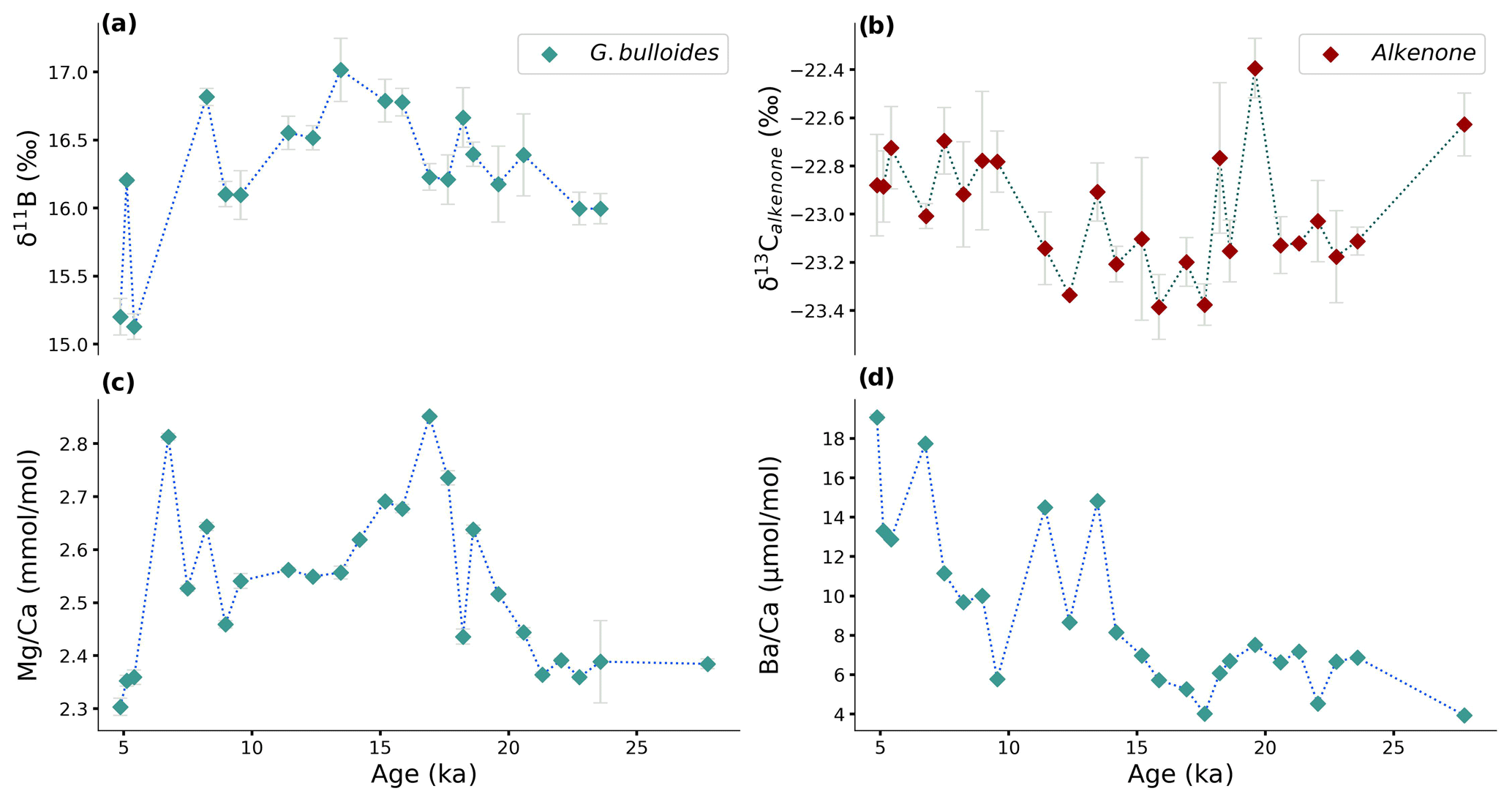
Figure 5 Measured (a) foraminiferal δ¹¹B, (b) alkenone δ¹³C, and foraminiferal element concentrations (c) Mg $/$ Ca (d) Ba $/$ Ca plotted over the past 27.8 kyr at the Benguela Upwelling System. Error bars show ± 1σ standard deviation. When error bars are not shown, the error of the duplicate measurement is smaller than the symbol.

The boron isotopic composition of the planktonic foraminifer, G. bulloides, ranges between 15.1 ‰ and 17.0 ‰ (relative to NIST 951), with larger variations during the last 6–5 kyr (Fig. 5a). The lowest δ¹¹B values were observed at 5.4 ka, whereas δ¹¹B values reach a maximum at 13.5 ka. Prior to this maximum value, δ¹¹B values show an increasing trend from 27.8 to 13.5 ka (Fig.  5a).

The carbon isotopic composition of the alkenones shows its heaviest value (−22.4 ‰) at 19.6 ka. After this peak, δ¹³C values reach a minimum (−23.4 ‰) at 15.9 ka then increased again towards the most recent values (−22.7 ‰ to −22.9 ‰; Fig. 5b).

5.3 Element $/$ Ca ratios in the planktonic foraminifer, G. bulloides

Mg $/$ Ca reaches maximum values of 2.85 and 2.81 mmol mol⁻¹ at 16.9 and 6.7 ka, respectively (Fig. 5c). Substantially lower values characterize the interval between 16.9 and 6.7 ka, when Mg $/$ Ca ranges between 2.46 and 2.69 mmol mol⁻¹. The lowest values (2.30–2.40 mmol mol⁻¹) were found at 4.9–5.4 ka and 21.3–27.8 ka.

The general trend in foraminiferal Ba $/$ Ca shows an increase from glacial to recent (Fig. 5d). The oldest part of the record shows relatively stable Ba $/$ Ca values at around 6 µmol mol⁻¹. During the last 15 kyr, however, more variability is observed for Ba $/$ Ca. The highest Ba $/$ Ca value (19.1 µmol mol⁻¹) is observed at the top of the record, and the lowest values, 4.02 and 3.94 µmol mol⁻¹, are observed at 17.6 and 27.8 ka, respectively.

5.4 U${}^{K_{\mathrm{37}}^{\prime }}$ sea surface temperatures

The alkenone-based U${}_{\mathrm{37}}^{K^{\prime }}$ record shows a continuous increase throughout the deglaciation (Fig. S3). The lowest value (0.56) was measured at 27.8 ka and increases to 0.58 until 23.6 ka. The interval of 22.0–19.6 ka again records low U${}_{\mathrm{37}}^{K^{\prime }}$ values, which then follows a steady increase until 9.6 ka. During the early Holocene, U${}_{\mathrm{37}}^{K^{\prime }}$ values stabilize around 0.7 until 6.8 ka, when values slightly start to decrease, reaching 0.67 in the uppermost part of the record.

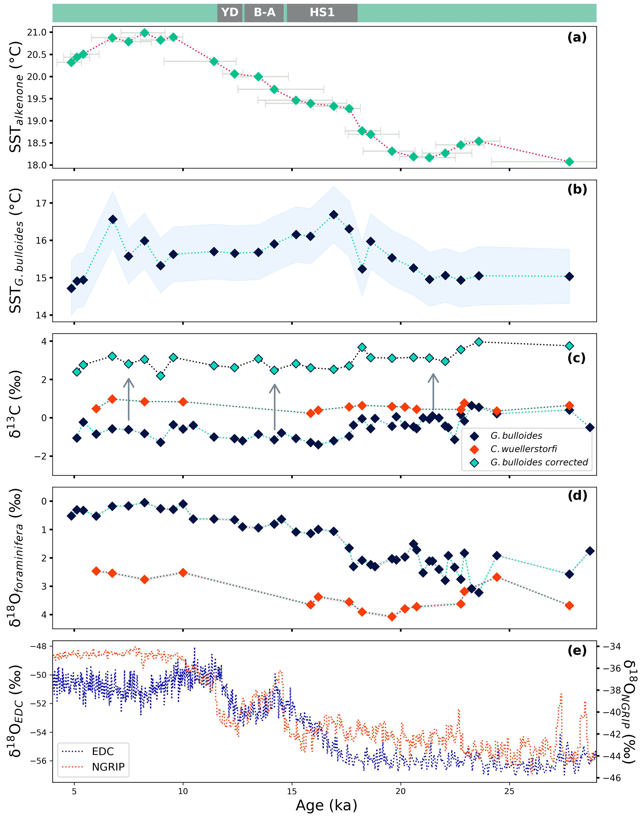
Figure 6 Reconstructed sea surface temperatures (SSTs) based on (a) the alkenone unsaturation index, U${}_{\mathrm{37}}^{K^{\prime }}$, and (b) foraminiferal Mg $/$ Ca; (c) δ¹³C analyzed in benthic (C. wuellerstorfi) and planktonic (G. bulloides) foraminifera with corrected values; (d) δ¹⁸O of benthic (C. wuellerstorfi) and planktonic (G. bulloides) foraminifera; and (e) the δ¹⁸O ice core record from EPICA Dome C (EDC; Jouzel et al., 2007) and the North Greenland Ice Core Project (NGRIP; North Greenland Ice Core Project Members, 2004) shown for the past 29 kyr. Corrected δ¹³C values of G. bulloides marked with green diamonds in panel (c) are based on temperature (derived from Mg $/$ Ca ratios; Bemis et al., 2000) and [CO${}_{\mathrm{3}}^{\mathrm{2}-}$] values (derived from pH and TA; Bijma et al., 1999), and arrows indicate the direction of the correction. The modern-day SST at core site 64PE450-BC6-PC8 is approximately 20.7 °C (GLODAPv2023; Lauvset et al., 2024; Santana-Casiano et al., 2009). Major climate events (YD: Younger Dryas; B–A: Bølling–Allerød interval; HS1: Heinrich Stadial 1) are marked above the top panel as reference. Horizontal error bars in panel (a) show the age uncertainty based on the 95 % confidence interval of the calibrated age. The shaded blue area in panel (b) indicates the error propagated from temperature calibration uncertainty and the ± 1σ standard deviation of the duplicate measurement of the samples. Analysis of the stable isotopes (c, d) provided an error smaller than the symbols shown in the figure.

6 Discussion

6.1 Local temperatures over the Last Glacial Maximum (LGM), last deglaciation, and Holocene

The proxy-based temperature reconstructions resemble the Southern Hemisphere climate responses based on the gradual temperature increase from 23 ka onwards (e.g., Petit et al., 1999; Suggate and Almond, 2005; Clark et al., 2009). However, comparing these reconstructions with both Northern Hemisphere (NGRIP; North Greenland Ice Core Project Members, 2004) and Southern Hemisphere (EPICA-Dome C; EDC; Jouzel et al., 2007) records, it is evident that individual climate events also show similarities to the trends observed in the Northern Hemisphere (Fig. 6). This suggests that the location of 64PE450-BC6-PC8 reflects a complex structure of the water column temperature, potentially affected by both Northern and Southern Hemisphere climatic changes.

The U${}_{\mathrm{37}}^{K^{\prime }}$-based sea surface temperature reconstruction shows low temperatures (18.2–18.5 °C) between 23.6 and 18.6 ka (Fig. 6a), which corresponds to the relatively low temperatures in the record based on the δ¹⁸O values from the shells of G. bulloides. These temperature minima and the relatively high variability (1.5 ‰–3.2 ‰) shown by the δ¹⁸O record between 24 and 21 ka indicate the Last Glacial Maximum (LGM; e.g., Clark et al., 2009; Hughes et al., 2013) within this record. While the trends observed here are in agreement with the general deglacial temperature records from higher latitudes, such a pattern is not reflected by the temperature record based on Mg $/$ Ca ratios of G. bulloides. In fact, the Mg $/$ Ca-based temperature trend is only between 23 and 16 ka comparable to the other local (U${}_{\mathrm{37}}^{K^{\prime }}$, foraminifera δ¹⁸O) and high-latitude reconstructions (ice core δ¹⁸O; e.g., Jouzel et al., 2007), after which this trend deviates from the classic deglacial pattern showing decreasing temperatures towards the Holocene.

While all these proxies have their inherent complications, the discrepancies between these records likely also reflect changes in the interaction between the core site and the higher latitudes. For instance, foraminiferal δ¹⁸O values not only depend on temperature, but also on the stable oxygen isotopic signature of the water and hence salinity. This may result in a signal of increasing temperatures in the U${}_{\mathrm{37}}^{K^{\prime }}$ and Mg $/$ Ca records, but not in the δ¹⁸O record (e.g., between 20 to 18 ka), due to a change in salinity that may compensate the impact of warming on δ¹⁸O values. Shifts in river runoff, for example, might also have impacted local seawater δ¹⁸O and hence foraminiferal oxygen isotopes. Similarly, multiple studies suggested an overall reduced Agulhas leakage during the LGM compared to deglacial levels (Pether, 1994; Flores et al., 1999; Rau et al., 2002; Peeters et al., 2004; Charles and Morley, 1988; Wefer et al., 1996; Franzese et al., 2006), and changes therein could also have resulted in enhanced δ¹⁸O variability during the LGM.

Not only the trends but also absolute values differ between the temperature reconstructions (i.e., U${}_{\mathrm{37}}^{K^{\prime }}$ and Mg $/$ Ca), which likely reflects a difference in water depth where the proxy signal carriers lived. Alkenone-based temperature reconstruction agrees with reported modern SSTs from the upper 50 m of the northern Benguela (Santana-Casiano et al., 2009), while the foraminifer-based temperature (Mg $/$ Ca) corresponds to the values observed somewhat deeper (100–150 m; GLODAPv2023; Lauvset et al., 2024; Fig. S4). The vertical dispersion of G. bulloides may be large, but the 100–150 m living habitat corresponds well with previously reported living depths for this species (Tapia et al., 2022; Lessa et al., 2020; Rebotim et al., 2017). The offset between U${}_{\mathrm{37}}^{K^{\prime }}$ and foraminiferal Mg $/$ Ca values during the LGM is about 3.0 °C, and this gradually increases to 5.6 °C during the early Holocene. This implies that foraminiferal Mg $/$ Ca values are affected by other factors than local SST alone. Partial dissolution of foraminiferal shells at depth may affect Mg $/$ Ca values and thereby bias reconstructed temperatures through the preferential loss of Mg²⁺ (Dekens et al., 2002; Regenberg et al., 2006). However, the impact of dissolution is probably minor only because the water depth at site 64PE450-PC8-BC6 is less than 1.4 km and G. bulloides is reported to be less sensitive to dissolution compared to other surface dwellers (Mekik et al., 2007). While Mg $/$ Ca values may also be affected by early diagenesis (Hover et al., 2001; Kozdon et al., 2013; Ni et al., 2020; Panieri et al., 2017; Sexton et al., 2006; Stainbank et al., 2020), El $/$ Ca ratios in the shell's profile obtained through laser ablation did not show any evidence for such diagenetic effects.

Inconsistent trends and minor changes in absolute temperature values over the last 27 kyr in this record make it challenging to identify millennial-scale climate events with confidence. The last deglacial was marked by large climate fluctuations primarily linked to the release of meltwater in the Northern Hemisphere weakening Atlantic Meridional Overturning Circulation (AMOC; McManus et al., 2004; Rahmstorf, 2002; Denton et al., 2010; Hodell et al., 2017; Pöppelmeier et al., 2023). This, in turn, changed global heat distribution causing cooling in the North Atlantic region that may have been accompanied by warming in the Southern Hemisphere (Broecker, 1998; Stocker, 1998). Such well-known climate events include Heinrich Stadial 1 (HS1; ∼ 17.8–14.5 ka; e.g., Bond et al., 1993; Cacho et al., 1999; McManus et al., 1994; Calvo et al., 2007; Wang et al., 2013) and the Younger Dryas (YD; ∼ 12.8–11.6 ka; Rühlemann et al., 1999; Kaplan et al., 2010; Panmei et al., 2017; Blunier and Brook, 2001; Alley, 2000), which were interrupted by a warming known as the Bølling–Allerød (B–A) Northern Hemisphere warming (∼ 14.6–12.9 ka; e.g., Pedro et al., 2016; Blunier et al., 1997; Lamy et al., 2007; Vandergoes et al., 2008). While high-latitude Southern Hemisphere records present warming signals during HS1 and YD, our temperature records remain relatively constant at the time of these events, and only the alkenone-based temperatures indicate slight warming at 12.4–11.4 ka. Deviating trends shown by the different proxy signal carriers are evident at the time of the B–A Northern Hemisphere warming, when Southern Hemisphere temperature reconstructions are also inconsistent at other locations (Lamy et al., 2007; Vandergoes et al., 2008).

Comparing the trends observed in the different proxies points to the dynamic glacial–deglacial history of the BUS, which was likely shaped by a varying influence of southern- and northern-sourced waters. Also, minor offsets might be explained by changes in either seasonality between haptophytes and G. bulloides (Leduc et al., 2010) or differences in water depth where the signals were recorded. Hence, such differences between the records could be due to a shift in productive season and/or a shift in depth habitat. As unraveling these signals is highly speculative, we focus on the glacial vs. interglacial contrasts observed.

6.2 Biological carbon pump

Comparing benthic (C. wuellerstorfi) and planktonic (G. bulloides) trends in δ¹³C shows they have similar values during the last glacial and higher δ¹³C values for the benthic than for the planktonic foraminifera during the interglacial. This is in contrast to what would be expected if BCP determined the foraminiferal carbon isotope signatures (Hain et al., 2014; Hilting et al., 2008). Generally, DIC in surface waters is enriched in ¹³C, as the BCP results in preferential export of ¹²C-rich organic matter to the deeper water masses, where it is released through remineralization. The efficiency and strength of the BCP is known to be affected by multiple processes, such as the formation, sinking, and interaction of aggregates with other minerals (Fowler and Knauer, 1986; Alldredge and Silver, 1988; Armstrong et al., 2001; Francois et al., 2002; Klaas and Archer, 2002; De La Rocha and Passow, 2007; Turner, 2015), and the efficiency is generally reflected by the offset in ¹³C between the surface and deep water (Δδ¹³C). However, species-specific offsets from equilibrium values between seawater DIC δ¹³C and foraminiferal carbonate δ¹³C can challenge interpretation of the Δδ¹³C and are likely responsible for the lower δ¹³C values of G. bulloides compared to C. wuellerstorfi observed here.

Application of foraminiferal Δδ¹³C as their proxy for BCP efficiency requires a direct relation with the δ¹³C of DIC. Benthic foraminiferal δ¹³C values, and, in particular δ¹³C values of the epifaunal C. wuellerstorfi, are generally considered faithful recorders of the δ¹³C values of DIC, with carbonate δ¹³C values being close to equilibrium (Thomas and Shackleton, 1996; Hilting et al., 2008). The stable carbon isotopic composition of DIC today is approximately 0.5 ‰–0.7 ‰ at a depth of 1.3 km along the latitude 20° S (Kroopnick, 1980; Kroopnick, 1985; Sarnthein et al., 1994; Curry and Oppo, 2005; Schmittner et al., 2013), which agrees well with the value inferred from C. wuellerstorfi in the uppermost sample (6.0 ka) of core 64PE450-BC6-PC8.

Stable carbon isotopic values from planktonic foraminifera have been shown to be generally lower with respect to the equilibrium values of DIC (Kahn, 1979; Kahn and Williams, 1981; Oppo and Fairbanks, 1989; Spero, 1992), indicating a strong biological impact (i.e., the vital effect; e.g., Spero, 1992; de Nooijer et al., 2014; Erez, 2003). For instance, symbiont-bearing species such as O. universa and T. sacculifer show offsets in δ¹³C as much as 1.8 and 1.4 ‰, respectively, depending on irradiance level (Spero, 1992; Spero and Lea, 1993). Although G. bulloides lacks algal symbionts (Hemleben et al., 1989), it has been shown to deviate even more from the ambient seawater δ¹³C values (Kahn and Williams, 1981; Spero and Lea, 1996). Several factors likely add together to the observed offset, such as carbon chemistry ([CO${}_{\mathrm{3}}^{\mathrm{2}-}$]; Spero et al., 1997; Bijma et al., 1999), temperature (Bemis et al., 2000), and respiration (Zeebe et al., 1999). The range of [CO${}_{\mathrm{3}}^{\mathrm{2}-}$] and temperature observed within our 27 kyr record may yield a δ¹³C offset of 0.6 ‰–1.4 ‰ and 2.4 ‰–2.6 ‰, respectively. More recently, Bird et al. (2017) suggested that bacterial symbiosis may also partly explain the observed offset for δ¹³C in G. bulloides. While symbiont photosynthesis contributes to elevating foraminiferal δ¹³C due to preferential ¹²C removal, the geochemical signature of G. bulloides is more likely to be controlled by the respiration of photoautotrophic cyanobacteria that produce depleted CO₂ and hence decrease shell δ¹³C values (Bird et al., 2017). Irrespective of the process involved, a substantial correction has to be applied to the δ¹³C values of G. bulloides to approach the heavier seawater DIC δ¹³C values. Increasing temperature (Bemis et al., 2000) and [CO${}_{\mathrm{3}}^{\mathrm{2}-}$] (Bijma et al., 1999) will also increase the offset between δ¹³C values of G. bulloides and seawater [DIC], suggesting that larger corrections are required during the Holocene than during the last glacial. Still, when the corrections for changes in temperature and [CO${}_{\mathrm{3}}^{\mathrm{2}-}$] are applied individually or combined, trends remain the same, showing the highest δ¹³C values of planktonic foraminifera during the LGM (Fig. S5). Hence, despite the uncertainties in interpreting the absolute planktonic δ¹³C values, the trend in Δδ¹³C should still provide a measure for changes in the efficiency of the BCP. Therefore, we applied a combined correction for both temperature (Bemis et al., 2000) and [CO${}_{\mathrm{3}}^{\mathrm{2}-}$] (Bijma et al., 1999), derived from foraminiferal Mg $/$ Ca and δ¹¹B, respectively (Fig. 6c). The offset of the δ¹³C value of the core-top sample with the modern δ¹³C values of the DIC is approximately 2.4 ‰ (Kroopnick, 1985), which agrees with the applied corrections based on temperature and [CO${}_{\mathrm{3}}^{\mathrm{2}-}$] in the most recent samples (2.4 ‰–2.8 ‰; 4.9–5.4 ka).

Offsets between the δ¹³C of the planktonic and benthic foraminifera reflect differences in the BCP but potentially also changes in the dominant water mass at the cores' locations. Intermediate depths of the South Atlantic are dominated today by the Antarctic Intermediate Water, and this likely remained the major water mass over the last glacial cycle (Pahnke et al., 2008; Howe et al., 2016; Gu et al., 2017). However, it is unclear whether the depth range of the AAIW increased (Muratli et al., 2010) or decreased (Ronge et al., 2015; Li et al., 2021) during the LGM compared to the present day. In the western Atlantic, δ¹³C values of benthic foraminifera suggest the persistence of AAIW masses at the depth of our core site (e.g., Curry and Oppo, 2005). As our values correspond to those found in the western Atlantic (Curry and Oppo, 2005; Lacerra et al., 2019; Umling et al., 2019), a sustained influence of southern water masses is likely, with the δ¹³C value of DIC in the AAIW during the LGM remaining relatively similar to the present day.

Variations in the stable carbon isotopic composition of surface seawater DIC are attributed to the changes in biological activity and air–sea exchange (Lynch-Stieglitz et al., 1995). While enhanced biological activity will result in an increase in δ¹³C values of DIC, more intense air–sea exchange will contribute to a decrease. In upwelling regions, the upwelled light carbon may still result in a net decrease in δ¹³C values despite the enhanced biological activity. The analyzed δ¹³C values of benthic foraminifera from the LGM in this study show on average values that are 0.2 ‰ lower than those during the Holocene, with a minimum glacial to a maximum Holocene range of 0.4 ‰–1 ‰. This increasing trend in mid-depth benthic δ¹³C values from glacial to interglacial agrees with the trends reported from the Brazilian Margin, where potentially both air–sea CO₂ exchange (Umling et al., 2019) and remineralization (Lacerra et al., 2019) affect the δ¹³C signal. Estimates of [PO${}_{\mathrm{4}}^{\mathrm{3}-}$] based on foraminiferal Ba $/$ Ca show a general increase from glacial to interglacial, with relatively low values between 18 and 15 ka corresponding to the observed planktonic δ¹³C minimum (Fig. S6). Although we cannot rule out a contribution of air–sea gas exchange, especially on the timescale of short-term climatic changes, we believe that the observed glacial–interglacial trend was primarily driven by a change in the BCP efficiency.

Summarizing the observed impacts, assuming a more or less stable presence of AAIW at intermediate depth and minimal impact of change in air–sea CO₂ exchange on δ¹³C values, after correcting for offsets, a larger difference between planktonic and benthic foraminiferal δ¹³C values during the LGM compared to the Holocene is evident (Figs. 6c and S5), suggesting a more efficient BCP.

6.3 pCO₂ record of the BUS over the last 27 kyr

Although δ¹¹B in foraminifera shells and δ¹³C of alkenones are the most commonly applied methods to reconstruct pCO₂, these proxies are only very rarely compared in the same record. Since these proxies record different components of the speciation of carbon in seawater and have different biases, they do not necessarily have to show similar results. Here, we observe only a modest change in pH (8.08–8.23 ± 0.07, derived from foraminiferal δ¹¹B) during the last deglaciation, whereas pCO₂ values show a change from 180 to 280 ppm (±42 ppm, derived from δ¹³C of alkenones; Fig. 7).

Minor variability in pH was reported previously by Raitzsch et al. (2018) for the Walvis Ridge for the same time interval, although reconstructed pH values were slightly higher (0.10–0.14 pH units). Although only minor, the offset is in line with the core studied here being closer to the upwelling area, as the major upwelling area extends only about 200 km out of the coast today (Lutjeharms and Meeuwis, 1987; Lutjeharms and Stockton, 1987). With the lowest pH values in the core of the upwelling area and values increasing towards the open ocean, the trend in the offset between the two areas is minor but in the right direction.

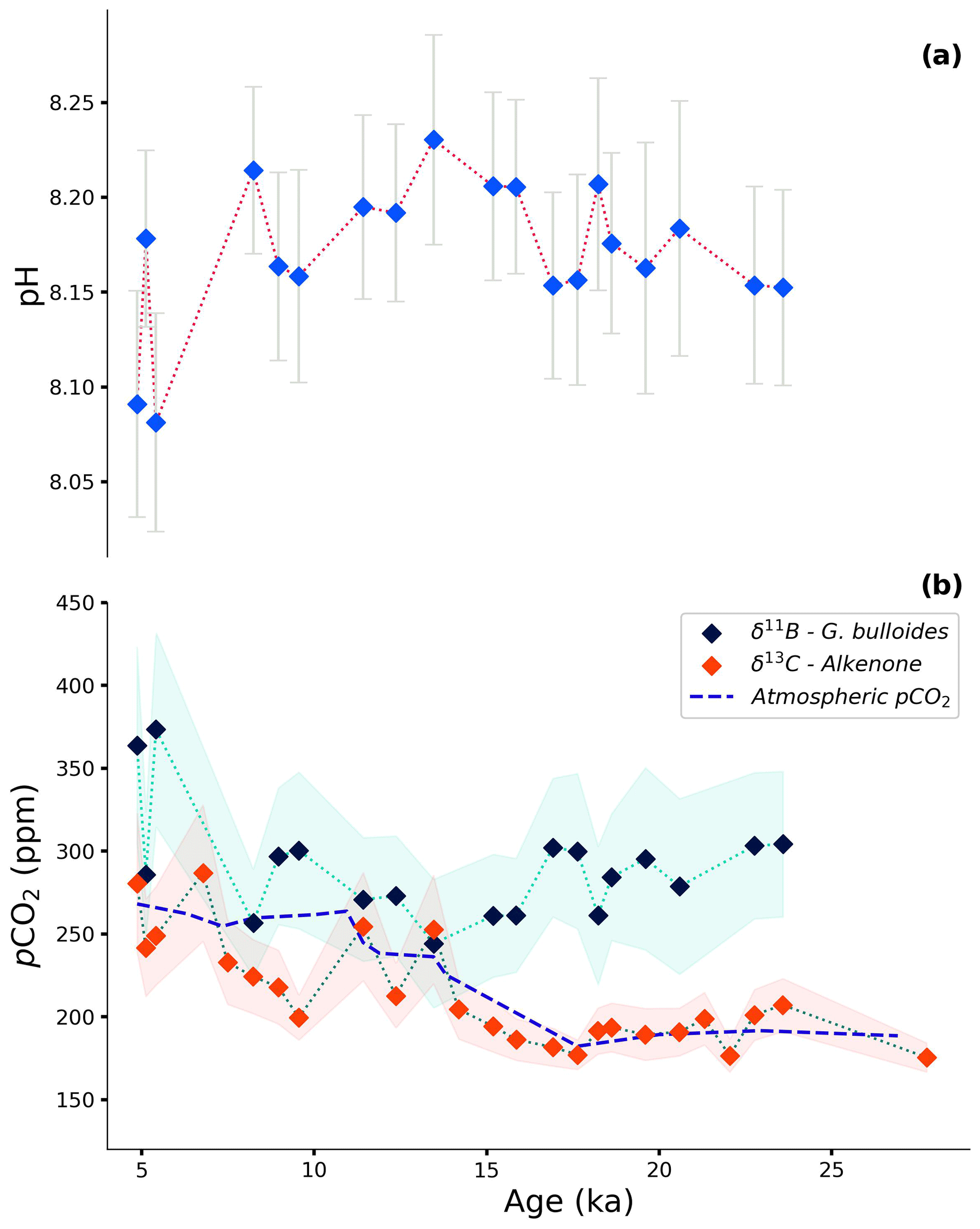
Figure 7 Reconstruction of (a) pH based on δ¹¹B of G. bulloides and (b) pCO₂ based on δ¹¹B of G. bulloides combined with a constant total alkalinity value of 2349 ± 11.07 µmol kg⁻¹ (dark-blue diamonds) and δ¹³C of alkenones with Ba $/$ Ca-based [PO${}_{\mathrm{4}}^{\mathrm{3}-}$] estimates (red diamonds). The modern-day pCO₂ value of the AAIW is approximately 326 ppm (Lauvset et al., 2024; Salt et al., 2015). The dashed blue line shows the Vostok ice core record of pCO₂ (Petit et al., 1999). The shaded light-green and red areas represent the propagated error for the foraminifera- and alkenone-based reconstructions, respectively. See further details on uncertainty propagation in the text.

Using pH and total alkalinity, pCO₂ can be calculated, suggesting higher pCO₂ compared to the known atmospheric values over the past 27 kyr (Fig. 7; Petit et al., 1999). Calculated pCO₂ based on the foraminiferal δ¹¹B only matches seawater equilibrium values at 13.5 and 8.2 ka. While the Bølling–Allerød event marks an AMOC amplification, AMOC was reduced around 8.2 ka due to the meltwater input in the North Atlantic (Matero et al., 2017; Barber et al., 1999; Pedro et al., 2016; Blunier et al., 1997). However, the calculated pCO₂ values are associated with considerable uncertainty for a large part related to total alkalinity being ill-constrained. Using estimates of total alkalinity based on relative sea level change is debated (e.g., de la Vega et al., 2023), as this does not account for all changes in alkalinity on glacial–interglacial timescales. Because total alkalinity calculated based on the relative sea level change during the last deglaciation results in only a small (less than 10 ppm) offset, we used constant alkalinity (2349 ± 11 µmol kg⁻¹; GLODAPv2023; Lauvset et al., 2024) in combination with boron-isotope-based pH to determine pCO₂. The trends observed here are not affected by the alkalinity values used.

The seawater pCO₂ reconstruction based on the δ¹³C of alkenones follows past atmospheric pCO₂, known from the Vostok ice core record, well (Petit et al., 1999). This suggests that, over the interval studied here, the BUS remained more or less in equilibrium with the atmosphere with regard to CO₂ and did not act as an appreciable source or sink. An offset is observed (about 65 ppm) during the Holocene, between 11 and 7 ka, when alkenone-based reconstruction suggests somewhat lower pCO₂ values compared to the ice core record, although this difference falls well within the uncertainty of the proxy. This could indicate a temporary transition of the area to a CO₂ sink as the seawater becomes undersaturated with respect to CO₂.

The good agreement between alkenone-based and ice core pCO₂ records suggests that previously recognized complications in applying this proxy may not be relevant in the BUS region. Adaptation of CCM by the alkenone producers can hamper the use of the proxy under low pCO₂ conditions (Badger, 2021). However, the mechanisms that may control CCM in the alkenone producers are not fully constrained (e.g., Reinfelder, 2011), and effectiveness of the CCM may differ between species (e.g., Goudet et al., 2020; Heureux et al., 2017). As the reconstruction of pCO₂ values based on alkenone δ¹³C provided a reasonable record here and in another upwelling region (Palmer et al., 2010), application of this proxy in upwelling sites may be able to rely on the classical concept of passive diffusion of CO₂ (Bidigare et al., 1997; Laws et al., 1995). Additional uncertainty in the alkenone-based pCO₂ reconstruction may derive from the estimation of the b factor. Often, modern and constant [PO${}_{\mathrm{4}}^{\mathrm{3}-}$] is assumed to estimate the b factor for reconstructing pCO₂ (Pagani et al., 1999; Zhang et al., 2013; Pagani et al., 2005; Witkowski et al., 2020), or, assuming that the membrane permeability has not changed significantly, one can correct for the growth rate effects of the alkenone producers (Zhang et al., 2019; Zhang et al., 2020). Here, we used foraminiferal Ba $/$ Ca, which is suggested to reflect nutrient ([PO${}_{\mathrm{4}}^{\mathrm{3}-}$]) variations but does not vary with temperature, salinity, or carbon chemistry parameters (Lea and Spero, 1994; Hönisch et al., 2011), unlike other suggested nutrient proxies, such as Cd $/$ Ca (Oppo and Rosenthal, 1994; Allen et al., 2016) and Zn $/$ Ca (Van Dijk et al., 2017). Using the Ba $/$ Ca approach to constrain the b factor yields 10 to 105 ppm lower pCO₂ values here compared to the approach of using a constant [PO${}_{\mathrm{4}}^{\mathrm{3}-}$] based on modern values over the last 27 kyr (Fig. S7). These approaches make a non-negligible difference to our conclusions, as the results based on the use of constant [PO${}_{\mathrm{4}}^{\mathrm{3}-}$] imply constant net CO₂ outgassing in the BUS over the last glacial and deglacial. However, variability in surface pCO₂ remains minor, causing only 32 ppm change in pCO₂ in the BUS over 27 kyr, which is unlikely considering the highly dynamic properties of the region on a glacial–interglacial timescale (Mollenhauer et al., 2002; McKay et al., 2016; Romero et al., 2003). Also, previous studies pointed out an overestimation of surface pCO₂ when constant nutrient levels are applied to constrain the b factor (Zhang et al., 2019, and references therein), which is in line with our observation when the two approaches (Ba $/$ Ca and constant [PO${}_{\mathrm{4}}^{\mathrm{3}-}$]) are compared. While the Ba $/$ Ca method still awaits refinements in future studies, this approach may provide an efficient way to address some of the uncertainties originating from local conditions that are not targeted when constant [PO${}_{\mathrm{4}}^{\mathrm{3}-}$] values are assumed.

6.4 Change in the efficiency of BCP and CO₂ disequilibrium

Most obvious from comparing the alkenone- and foraminifera-based pCO₂ reconstruction is the difference in amplitude of change on a glacial–interglacial timescale. While the alkenone-based reconstruction closely mimics atmospheric changes, the foraminifera-based reconstruction shows a constant pCO₂. This results in an interglacial difference in pCO₂(ΔpCO₂=pCO_{2(foraminifera)}− pCO_2(alkenone)) of about 64 ± 20 ppm between the alkenone- and foraminifera-based reconstructions, while, during glacial times, ΔpCO₂ increases to approximately 94 ± 20 ppm (Fig. 8). Because the G. bulloides are proliferating during the upwelling season, they likely primarily reflect the deeper upwelled water (i.e., subsurface) compared to the alkenones, which are synthesized, for example, by the surface-dwelling coccolithophorids. Note that G. bulloides may migrate between approximately 50 and 400 m (Rebotim et al., 2017), which can affect the calculated pCO₂ gradients. Still, G. bulloides represents a larger average depth than the alkenone-based record and hence carbon system conditions that are closer to those of the upwelled intermediate waters, i.e., the AAIW in the BUS.

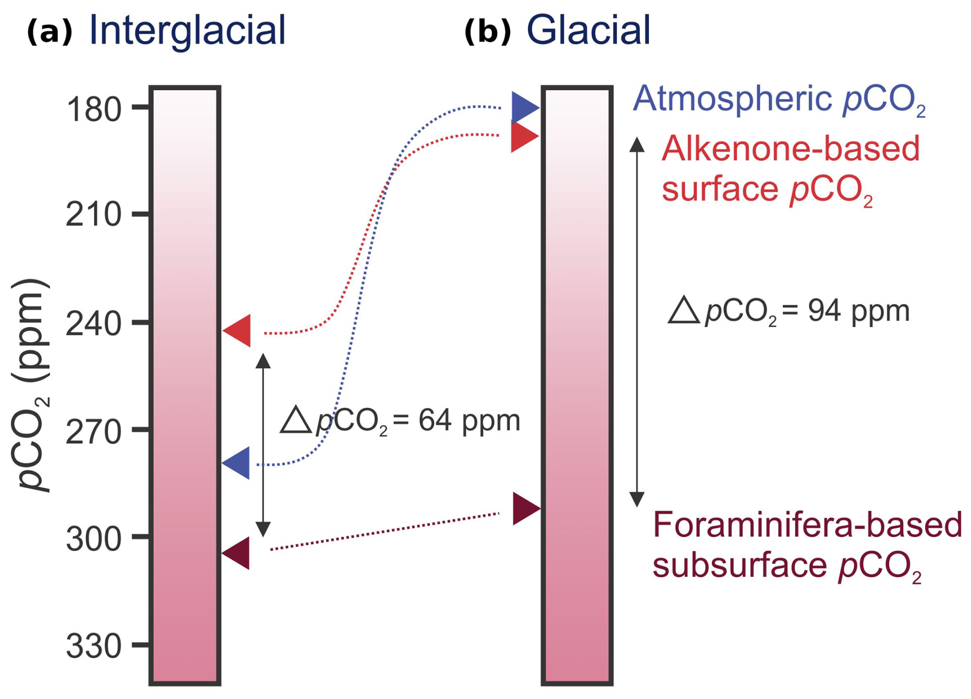
Figure 8 Schematic comparison of interglacial and glacial pCO₂ values. Red arrows mark average interglacial (a) and glacial (b) values calculated from the alkenone- and planktonic-foraminifera-based (pH and total alkalinity) proxies in this study.

Studies using foraminifera-based proxies suggested more intense upwelling during glacial times (Oberhänsli, 1991; Little et al., 1997), but, at the same time, radiolarian-based upwelling proxies indicate reduced upwelling (Des Combes and Abelmann, 2007). Due to its location and the influence of water masses both from the north and the south, cells of the BUS are characterized by different environmental conditions (e.g., temperature and nutrients; Emeis et al., 2018). During the LGM, cold source waters likely impacted the northern cells of the BUS more than its central and southern parts (Des Combes and Abelmann, 2007), affirming complexity of this upwelling system. While we may conclude that upwelling intensities were different from one cell to another, potentially also impacted by the offshore transition of the modern strong upwelling cells (e.g., Mollenhauer et al., 2002), increased cold water input does not necessarily correlate with stronger upwelling (Des Combes and Abelmann, 2007), potentially explaining conflicting interpretations based on different proxies.

Atmospheric pCO₂ was significantly reduced during the LGM; hence the presence of an increased amount of CO₂ at subsurface depths implies either enhanced upwelling or that the upwelled waters were richer in CO₂ or both. Lower atmospheric CO₂ during the glacial is likely explained by multiple processes. The larger extent of sea ice over the glacial Southern Ocean prevented CO₂ escaping from seawater in an area today acting as a major CO₂ exchange region (Stephens and Keeling, 2000), whereas enhanced iron fertilization likely contributed to more efficient utilization and transport of carbon and nutrients to the deep (Martin, 1990; Martínez-García et al., 2014). Eolian transport and dissolution in the shelf regions might have provided important sources of iron at that time (Martin, 1990; Tian et al., 2023), which would locally influence air–sea carbon balance, still with minimum impact on global atmospheric pCO₂ due to adjacent regions where excess carbon can be utilized. Also locally at the BUS, eolian transport presumably increased due to the intensified trade winds (Stuut et al., 2002), although a more humid climate may (Stuut et al., 2002; Cockcroft et al., 1987) or may not (Shi et al., 1998; Partridge et al., 1999) have prevailed in southwestern Africa during the LGM. Therefore, it remains speculative whether stronger winds may have provided sufficient iron for phytoplankton growth locally or if excess iron input in the sub-Antarctic region potentially provided a source for additional mid-depth CO₂ storage (Martínez-García et al., 2014). Still, a more efficient biological carbon pump, as indicated by the offset between the planktonic and benthic foraminiferal carbon isotope records (Fig. 6c), suggests that an increased supply of carbon in the upwelling areas from intermediate depths to the surface may have been effectively counterbalanced.

Based on comparing pCO₂ proxies, with G. bulloides primarily recording the upwelled waters and alkenones primarily recording the surface waters, we see evidence for enhanced storage of carbon at depth during the glacial. The resulting mid-depth high-CO₂ waters also provide the source for upwelled waters in the BUS at that time, which could have resulted in the local release of (part of the) stored CO₂ if not prevented by an efficient biological carbon pump. An increased biological pump acted as an effective cap on the stored carbon and hence contributed to preventing the release of mid-depth CO₂ during the glacial.

7 Conclusions

Carbon system proxies were applied to demonstrate changes in inorganic carbon chemistry of the northern Benguela Upwelling System over the last 27 kyr. Temperature reconstructions based on both organic and inorganic proxies indicate that the BUS may be associated with climatic changes observed in both the Northern and Southern hemispheres. While surface values of pCO₂ reconstructed from δ¹³C of alkenones generally track atmospheric pCO₂, the foraminifera-based reconstruction suggests minor variation in pCO₂ in the subsurface since the Last Glacial Maximum until the present. Hence, the increased gradient of pCO₂ between the surface waters and depth observed for the last glacial period provides evidence for enhanced storage of carbon in the Antarctic Intermediate Water. Outgassing of CO₂, however, could be effectively prevented by the biological carbon pump, as also indicated by the offset in the δ¹³C of planktonic and benthic foraminifera.