Shifts in Greenland interannual climate variability lead Dansgaard–Oeschger abrupt warming by hundreds of years

During the Last Glacial Period (LGP), Greenland experienced approximately 30 abrupt warming phases, known as Dansgaard–Oeschger (D–O) events, followed by cooling back to baseline glacial conditions. Studies of mean climate change across warming transitions reveal indistinguishable phase offsets between shifts in temperature, dust, sea salt, accumulation, and moisture source, thus preventing a comprehensive understanding of the “anatomy” of D–O cycles (Capron et al., 2021). One aspect of abrupt change that has not been systematically assessed is how high-frequency interannual-scale climatic variability surrounding centennial-scale mean temperature changes across D–O transitions. Here, we utilize the East Greenland Ice-core Project (EGRIP) high-resolution water isotope record, a proxy for temperature and atmospheric circulation, to quantify the amplitude of 7–15-year isotopic variability for D–O events 2–13, the Younger Dryas, and the Bølling–Allerød. On average, cold stadial periods consistently exhibit greater variability than warm interstadial periods. Most notably, we often find that reductions in the amplitude of the 7–15-year band led abrupt D–O warmings by hundreds of years. Such a large phase offset between two climate parameters in a Greenland ice core has never been documented for D–O cycles. However, similar centennial lead times have been found in proxies for Norwegian Sea ice cover relative to abrupt Greenland warming (Sadatzki et al., 2020). Using HadCM3, a fully coupled general circulation model, we assess the effects of sea ice on 7–15-year temperature variability at the EGRIP. For a range of stadial and interstadial conditions, we find a strong relationship in line with our observations between colder simulated mean temperature and enhanced temperature variability at the EGRIP location. We also find a robust correlation between year-to-year North Atlantic sea ice fluctuations and the strength of interannual-scale temperature variability at EGRIP. Together, paleoclimate proxy evidence and model simulations suggest that sea ice plays a substantial role in high-frequency climate variability prior to D–O warming. This provides a clue about the anatomy of D–O events and should be the target of future sea ice model studies.

1 Introduction

1.1 Dansgaard–Oeschger events

Stable isotopes of hydrogen (δD) and oxygen (δ¹⁸O) in polar ice cores provide information about local temperature and atmospheric circulation (Dansgaard, 1964). In Greenland, measurements of δ¹⁸O and δD during the Last Glacial Period (LGP; 115–12 ka) reveal recurrent alternations, referred to as Dansgaard–Oeschger (D–O) cycles, between quasi-stable warm periods (i.e., Greenland interstadials, GIs) and cold baseline conditions (i.e., Greenland stadials; GSs) (Dansgaard et al., 1993). Global climate change associated with GI phases includes increased aridity across North America and Eurasia (Wagner et al., 2010; Asmerom et al., 2010), a northward shift in the tropical rain belt (Cruz et al., 2005; Deplazes et al., 2013), and antiphase warm periods in Antarctica (Blunier et al., 1998; Blunier and Brook, 2001; EPICA Community Members, 2006). It is widely accepted that these changes are linked via fluctuating strengths of the Atlantic Meridional Ocean Circulation (AMOC) in which GI and GS phases are characterized by strong and weak overturning, respectively (Broecker, 1998; Knutti et al., 2004; Stocker and Johnsen, 2003). Abrupt GS–GI transitions have received widespread attention due to the unusual rate and magnitude of climatic change. For example, Greenland temperature increases of 5–16.5 °C occurred in a matter of decades (Huber et al., 2006; Kindler et al., 2014; Severinghaus et al., 1998; Severinghaus and Brook, 1999). Despite decades of research, the trigger of this phenomenon and associated global changes is still debated.

1.2 Sea ice

North Atlantic sea ice is often referenced in explanations of D–O warming because of its rapid response to relatively weak forcing and its influence on both atmospheric and oceanic dynamics. Several model simulations (Li et al., 2005, 2010; Boers et al., 2018; Dokken et al., 2013; Petersen et al., 2013) show that sea ice displacements in the North Atlantic and Nordic seas, complemented by associated feedbacks, can produce abrupt temperature increases consistent with those documented by water isotopes in Greenland ice cores. Though model reconstructions vary slightly, a primary mechanism for abrupt warming includes initial sea ice reductions amplified by oceanic heat loss to the atmosphere, perturbations to the ocean salinity gradient, and decreased surface albedo.

Determining the driver(s) of sea ice displacements, in relation to abrupt Greenland warming, requires a highly resolved chronology of pertinent regional changes. Biomarker evidence from ocean sediment cores confirms that sea ice in the southern Norwegian Sea consistently experienced millennial-scale oscillations in pace with D–O cycles (Hoff et al., 2016). In one core location, ice cover reductions began during the late GS phase, thus leading to abrupt warming by hundreds of years (Sadatzki et al., 2019, 2020). However, these ocean sediment cores have low resolution (i.e., multi-decadal-scale sampling), and their age chronologies have large uncertainties. By comparison, Greenland ice cores can reach annual or multi-year resolution. For this reason, they have been key in establishing leads and lags of various geological parameters, deducing causal relationships, and disentangling the spatiotemporal progression of abrupt climate change. Observations of dust, moisture source, and accumulation during D–O warming exhibit indistinguishable (Capron et al., 2021) or near-synchronous (Steffensen et al., 2008) shifts, suggesting that widespread regional climate changes in the North Atlantic and Greenland occurred in-phase. This is partly at odds with evidence from Norwegian Sea sediment cores.

1.3 Climate variability

To further investigate leads and lags during abrupt D–O warmings, we utilize the East Greenland Ice-core Project (EGRIP) water isotope (δD) record to assess the temporal evolution of mean temperature vs. high-frequency water isotope variability in northeastern Greenland. Variability in Greenland ice cores has long been studied, but coarse analytical sampling on increasingly compressed annual ice layers has limited LGP analyses to centennial or millennial scales (WAIS Divide Project Members, 2015; Rehfeld et al., 2018; Schulz et al., 2004). Similarly, interpretations of interannual- and decadal-scale Greenland climate variability have primarily been available for the Holocene (11.7–0 ka) (Hughes et al., 2020; Rimbu and Lohmann, 2010; Rimbu et al., 2021; Ortega et al., 2014). Though studies assessing decadal-scale variability during the LGP exist (Boers et al., 2018; Ditlevsen et al., 2002), the data sets used were discretely sampled at centimeter-scale resolutions, which may diminish or conceal important high-frequency climatic information (Fig. A1). Developments in continuous-flow sampling techniques have recently allowed for high-frequency analysis of water isotope variability in Antarctic ice cores during the LGP by preserving the amplitude of interannual-scale signals (Jones et al., 2017a, 2018). In the case of West Antarctica, a shift in LGP interannual isotopic variability was linked to broad changes in Pacific basin teleconnection strength driven by reductions in the Laurentide Ice Sheet topography and changing albedo (Jones et al., 2018). This study demonstrated that the drivers of high-frequency climate variability can temporally decouple from the drivers of mean local climate (temperature, accumulation, etc.), providing new insights about paleoclimate dynamics.

In the northern high latitudes, sea ice varies substantially on multi-year and multi-decade bases, imparting variability into the climate system on similar timescales. The Greenland water isotope variability record may therefore provide clues about high-frequency sea ice variations as such shifts would affect the isotopic signature of precipitation via influences on both moisture source and atmospheric circulation. Our study comprises four parts: (1) comparison of LGP isotopic variability relative to the Holocene; (2) comparison of isotopic variability between warm Greenland interstadials (GIs) and cold Greenland stadials (GSs); (3) a moving window assessment of lead–lag relationships between isotopic variability and mean temperature increases associated with D–O events; and (4) a model assessment of LGP North Atlantic temperature and sea ice variability at interannual scales using the general circulation model HadCM3, including how simulated sea ice variability affects temperature variability at the EGRIP site.

2 Methods

2.1 Water isotope data

The EGRIP ice core was drilled at 75° 38^′ N and 35° 60^′ W from an interior location of the Northeast Greenland Ice Stream (NEGIS). Due to rapid ice flow in this location, glacial portions of the EGRIP ice core originate ∼ 200 km upstream near the Greenland ice sheet divide (Gerber et al., 2021). δD and δ¹⁸O records were measured using a semi-automated continuous-flow analysis (CFA) system in conjunction with a Picarro cavity ring-down laser spectrometer (CRDS; model L2130-i) (Jones et al., 2017a). The CFA–CRDS system constitutes three subsystems: the ice core melter, a liquid phase to vapor phase conversion, and the isotopic analyzer. Ice core sticks measuring $\mathrm{100}\times \mathrm{1.3}\times \mathrm{1.3}$ cm are melted at a rate of 2.5 cm min⁻¹ by an aluminum plate maintained at 14.6° C. Meltwater is pulled through the preparation line via peristaltic pumps, where it is filtered to remove particulates, degassed, and aerosolized by a nebulizer. Finally, ice-core-derived water vapor is introduced to the CRDS in a continuous, stable stream for optimal performance. Precise δD and δ¹⁸O measurements are derived in real time relative to Vienna Standard Mean Ocean Water (VSMOW; δ¹⁸O = δD = 0‰). Using this CFA methodology, the water isotope record has a sample resolution of ∼ 1 mm throughout, with an effective resolution of ∼ 5 mm due to mixing. Figure A1 demonstrates the artificial loss of interannual amplitudes with depth for coarser (i.e., centimeter-scale) sampling resolutions.

To date, the EGRIP water isotope record extends to ∼ 49.9 ka b2k (thousands of years before 2000 CE) according to the Greenland Ice Core Chronology (GICC05) (Svensson et al., 2008) (Fig. 1a). The GICC05 was transferred to EGRIP using 373 tie points between 0–14.96 ka b2k (Mojtabavi et al., 2020) and an additional 138 tie points between 14.96–49.9 ka b2k (Gerber et al., 2021). For each EGRIP data point (in millimeter resolution), the corresponding North Greenland Ice Core Project (NGRIP) depth was obtained by linear interpolation between the tie points, and the age was determined from the annual-layer-counted GICC05 timescale. The ages used here inherit the maximum counting error in the GICC05 timescale. In addition, the interpolation introduces an uncertainty which is relevant when comparing to other records on the GICC05 timescale. Isotope data are interpolated at a uniform time interval of 0.05 years. On average, temporal differences in adjacent data points (i.e., next to one another) range from sub-weekly in the Holocene to sub-monthly during the LGP.

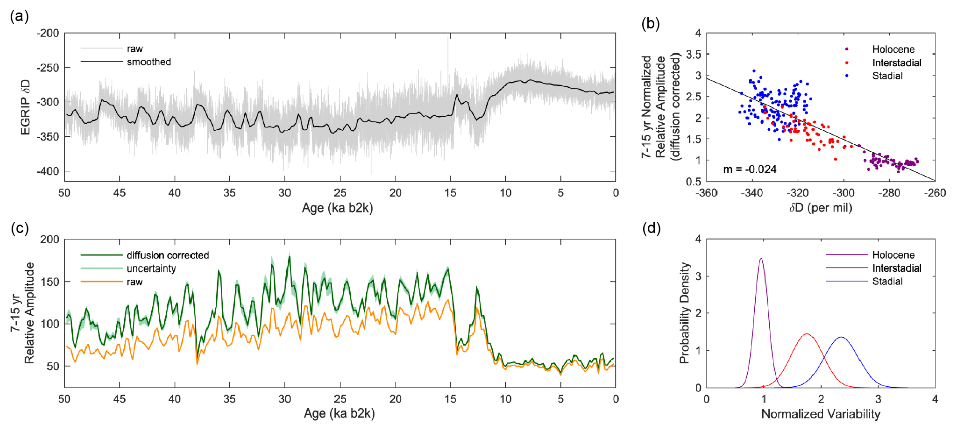
Figure 1 (a) EGRIP δD to 50 ka b2k (grey) overlaid by downsampled data for visual clarity (black; window = 400 years; time step = 200 years). (b) Diffusion-corrected data from panel (c) binned by climate state and fit with linear regression (r²=0.75; p<0.05). (c) Raw (orange) and diffusion-corrected (green) strength of the 7–15-year isotopic variability at EGRIP (window = 400 years; time step = 200 years). (d) Variance in binned data from panel (b).

2.2 Spectral analysis

We use a multi-taper method (MTM) of spectral analysis (Huybers, 2021; Percival and Walden, 1993) to calculate spectral power densities which are later converted to relative amplitudes within the 7–15-year band. MTM spectral analysis averages multiple realizations of data using a series of Slepian tapers, offering a smoothed estimate of prominent spectral characteristics. We spectrally analyze the EGRIP δD record in 400-year windows with a time step (i.e., stepwise shift between adjacent windows) of 50 to 200 years, depending on desired temporal resolution. A window size of 400 years provides adequate repetition of interannual to decadal signals for a precise estimation of high-frequency power density spectra.

2.3 High-frequency signal attenuation

Firn is a porous and permeable substance comprised of snow and ice at the surface of an ice sheet. Water vapor within interconnected firn pathways diffuses along temperature and concentration gradients. Isotopic exchange occurs at four interfaces (i.e., (1) vapor–vapor, (2) vapor–ice surface, (3) ice surface–ice interior, and (4) through the ice matrix, altering the isotopic composition of deposited precipitation) (Whillans and Grootes, 1985). Vapor phase diffusion disproportionately dampens high-frequency signals but ceases below a pore density of 804 kg m⁻³ (Johnsen et al., 2000). Solid-phase diffusion continues below the pore close-off depth at a considerably slower rate (Jones et al., 2017). Spectral analysis is used to interpret the extent of vapor phase and solid-phase diffusion to single-frequency bands (Fig. A2). At EGRIP, the annual signal (i.e., 1 year) cannot be resolved, while the 2–5-year signals are significantly dampened throughout the LGP and Holocene. The 7–15-year band is well preserved throughout the entire EGRIP record and is thus the focus of this analysis.

2.4 Gaussian diffusion correction

Values of cumulative mean water molecule diffusion, known as “diffusion lengths”, can be estimated for windows of time or depth along a water isotope signal by evaluating dampened sections of its high-frequency spectrum (Gkinis et al., 2014; Hughes et al., 2020; Johnsen et al., 2000, 2017b, 2018, 2023; Kahle et al., 2021; Simonsen et al., 2011). Diffusion lengths are equivalent to the estimated standard deviation (i.e., sigma) of water molecule diffusion, which describes the statistical vertical displacement of water molecules from their original position (Fig. A3; Johnsen et al., 2000). The power density spectrum of a diffused water isotope signal, P (f), is defined as

$$\begin{array}{}\text{(1)}& P\left(f\right)=P_{\mathrm{o}}\left(f\right)\exp {\left[-\left(\mathrm{2}\mathit{\pi }f{\mathit{\sigma }}_{\mathrm{a}}\right)\right]}^{\mathrm{2}},\end{array}$$

where P_o (f) is the power density spectrum of the undiffused signal (in units of ‰² yr), f is the frequency (in units of 1 yr⁻¹), and σ_a is the diffusion length (in units of years). To solve for σ_a, we create 12 equally spaced logarithmic bins within the diffused interval and fit a Gaussian to P(f) using a least squares fitting technique) (Fig. A4). The EGRIP δD diffused interval ranges between the 2–25-year band, and the Gaussian fit is optimized by manually adjusting this interval for each age window. This ensures the diffusion length is not calculated based on measurement noise, which occurs at an even higher frequencies and can be identified as a sudden bend in the slope of P(f). Diffusion lengths can be expressed in meters (σ_z) using the following conversion:

$$\begin{array}{}\text{(2)}& {\mathit{\sigma }}_{\mathrm{z}}={\mathit{\sigma }}_{\mathrm{a}}\cdot {\mathit{\lambda }}_{\mathrm{avg}},\end{array}$$

where λ_avg is the mean annual layer thickness (in units of m yr⁻¹). The diffusion-corrected power density spectra, P_o(f), is determined by rearranging Eq. (1) so that

$$\begin{array}{}\text{(3)}& P_{\mathrm{o}}\left(f\right)=P\exp \left[\mathrm{4}{\mathit{\pi }}^{\mathrm{2}}{f}^{\mathrm{2}}{\mathit{\sigma }}_{\mathrm{a}}^{\mathrm{2}}\right],\end{array}$$

where P is the observed power density, f is the frequency, and σ_a is the solved diffusion length. We calculate the average undiffused power density, P_ave, in the 7–15-year band by dividing the integral of power density by the frequency range (Jones et al., 2018) as follows:

$$\begin{array}{}\text{(4)}& P_{\mathrm{ave}}={\displaystyle \frac{\underset{f_{\mathrm{a}}}{\overset{f_{\mathrm{b}}}{\int }}{P}_{\mathrm{o}}\left(f\right)}{f_{\mathrm{b}}-f_{\mathrm{a}}}},\end{array}$$

where f_a and f_b are the upper and lower limits of the frequency band, respectively. Relative strength (P_amp), or amplitude, is calculated for each window as the square root of average power density (P_ave) as follows:

$$\begin{array}{}\text{(5)}& P_{\mathrm{amp}}=\sqrt{P_{\mathrm{ave}}}.\end{array}$$

2.5 Uncertainty

Diffusion length, σ_a, can be alternatively quantified as the slope, m, of a linear regression, y, fitted to ln[P(f)] versus f² of the diffused interval. Uncertainty bounds are defined as maximum and minimum slopes within 1 standard deviation of y (Jones et al., 2017b, 2018) (Fig. A4).

2.6 HadCM3

To investigate the physical processes underlying our results, we utilize the fully coupled HadCM3 ocean–atmosphere general circulation model (GCM) to test how global climate responds to various forcing mechanisms in the North Atlantic (Gordon et al., 2000; Pope et al., 2000; Valdes et al., 2017). The simulations used here (Roberts and Hopcroft, 2020) force LGP stadial phases through the imposition of a freshwater flux or a perturbation to annual mean sea ice cover. The hosing simulations impose freshwater uniformly across the North Atlantic between 50 to 70° N and include variations in flux between 0.04 and 1.0 Sv (10⁶ m³ s⁻¹). The perturbed sea ice simulations artificially pin ice extent to a particular latitude between 40 to 70° N, though interannual ice edge variability is still possible due to advection in the module. Ice depth is prescribed to 4 m and may reach a maximum concentration of 95 %. To deconvolve how climate responds to sea ice and freshwater hosing, a forcing which combines the aforementioned simulations is included. To investigate a possible dependence on the background climate state, we also impose the sea ice and freshwater forcing onto boundary conditions simulating the Last Glacial Maximum (LGM) and pre-industrial (PI). We calculate high-frequency interannual-scale variability as the standard deviation of 7–15-year band-pass-filtered time series for temperature and sea ice concentration output.

The freshwater hosing and pinned sea ice simulations give a range of mean temperatures at the location of EGRIP that represent a spectrum of possible mean LGP climate states. By including a spectrum, we reduce the bias that could arise from defining a single stadial or interstadial state with only one forcing mechanism. Both forcings alter the distribution of sea ice; however, the freshwater forcing also imposes a large, and potentially unrealistic, change on the ocean circulation. Crucially, including these two sets of simulations controls for oceanic-driven effects when investigating the role of sea ice in driving climatic variability at EGRIP; if a response is general across all simulations, even for pinned sea ice simulations with no change in ocean circulation, then we can infer that ocean circulation is not the immediate cause of the change.

3 Results

3.1 Interannual water isotope variability

The raw EGRIP δD record exhibits millennial-scale D–O variability consistent with prior analyses of deep-ice cores (e.g., GRIP and NGRIP) recovered from inland Greenland (Fig. 1a) (Greenland Ice-core Project (GRIP) Members, 1993; North Greenland Ice Core Project Members, 2004). Isotopic measurements range from approximately −240 ‰ to −310 ‰ in the Holocene, while the LGP is characterized by increased depletion and greater spread in values ranging from −260 ‰ to −380 ‰. On average, diffusion-corrected variability in the 7–15-year band is elevated during the LGP compared to the Holocene, reaching a maximum plateau between ∼ 30–15 ka b2k. The average decrease in variability between the plateau and the Holocene is approximately 60 % (Fig. 1b).

Large variations in the 7–15-year variability during the LGP are evident. For example, the 7–15-year amplitude at ∼ 38 ka b2k is so low that it is nearly the same magnitude as the variability seen throughout the Holocene. Conversely, the variability at ∼ 29.5 ka b2k is ∼ 360 % greater than in the Holocene. Another important detail is that the raw (i.e., non-diffusion-corrected) 7–15-year variability record exhibits lower amplitudes, yet simultaneous shifts with the corrected record (Fig. 1c). This demonstrates the ability of our correction to target signal attenuation by diffusion without incorporating uncertainty into the temporal evolution of the record. In other words, the signal we document is a robust feature of the climate system and not an artifact of the diffusion correction or laboratory analysis.

Within the context of the LGP, high-frequency variability is on average 18 % lower in the 400 years following the onset of warm GI periods, relative to the onset of preceding cold GS periods (Rasmussen et al., 2014) (Fig. 2b). The largest reduction in the variability from GS onset to GI onset is 37 % for D–O event 8, while the smallest change is indistinguishable from zero for D–O event 9. In the case of D–O event 9, the temporal length of the interstadial is only 260 years, which skews 400-year averages towards the background stadial state. There are no instances of greater variability during a GI onset relative to the prior GS onset (Table 1). The above analyses demonstrate a negative correlation between water isotope ratios (δD) (which are a proxy for temperature) and the strength (i.e., amplitude) of the interannual and decadal isotopic variability in northeastern Greenland throughout the last 50 kyr (Fig. 1c, d). It is important to note that we document multi-millennial excursions in the variability occurring between 27–15 ka b2k, where cold GS conditions persist uninterrupted by abrupt warming, with the exception of D–O event 2 at around 23 ka b2k. The excursions are comparable yet generally smaller in magnitude than those occurring between 50–27 ka b2k when D–O cycling is relatively consistent.

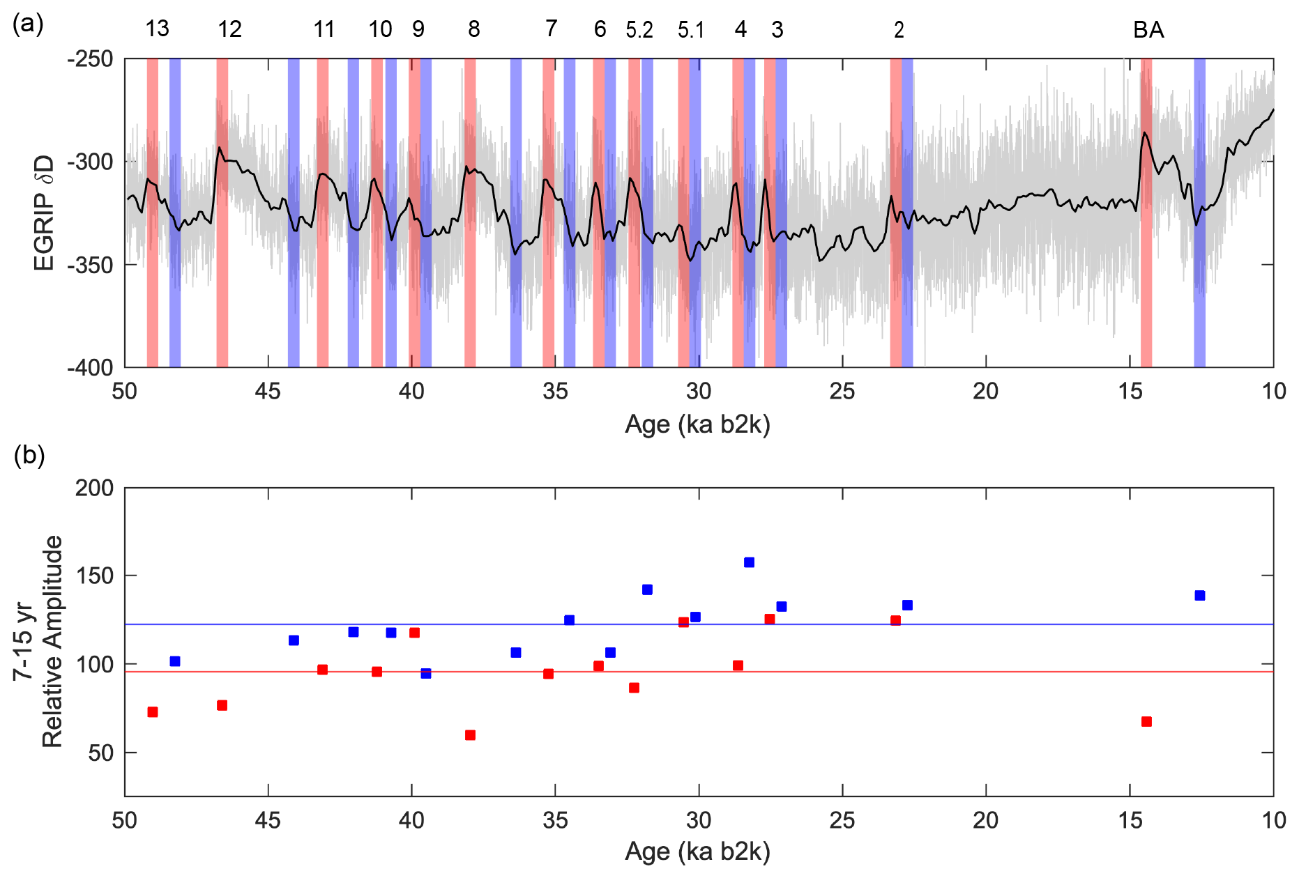
Figure 2 (a) EGRIP δD overlaid by 400-year windows at the onset of the Greenland interstadial (GI; red) and Greenland stadial (GS; blue) periods (Rasmussen et al., 2014). For GI phases shorter than 400 years, the onset of the subsequent GS phase is defined as the termination of the GI window to avoid overlap. Due to the brief duration of GI 2.1 and 2.2, one 400-year window is placed at the onset of GI 2.2 (i.e., 23.34 ka b2k), which encompasses the entirety of GI 2.2, the majority of GI 2.1, and the short-lived stadial phase between each interstadial. D–O events are indicated on the upper x axis (b) diffusion-corrected 7–15-year variability in the windows outlined in panel (a).

Next, we reduce the time step of our 400-year window analysis from 200 to 50 years to analyze the lead–lag relationship between mean temperature change associated with D–O events and isotopic variability (Fig. 3a, b). In most instances (i.e., D–O events 2, 3, 4, 5.1, 5.2, 6, 7, 8, 9, 10, 12, and 13), we find that the reduction in the 7–15-year variability from peak values initiates ∼ 150–600 years prior to abrupt warming (Fig. 4). For these events, approximately 50 % or more of the variability change has occurred before the abrupt warming begins, as defined by Rasmussen et al. (2014). There is only one case (i.e., D–O event 11) in which the reduction in the isotopic variability leads to warming on sub-centennial scales. Due to our window size of 400 years, we can only conclusively say that lead times of > 200 years are significant beyond uncertainty of the diffusion correction. Thus, there is clear evidence that 7–15-year variability for D–O events 2, 3, 4, 5.2, 6, 7, 8, 10, 12, and 13 leads centennial-scale mean temperature change at the onset of GI phases.

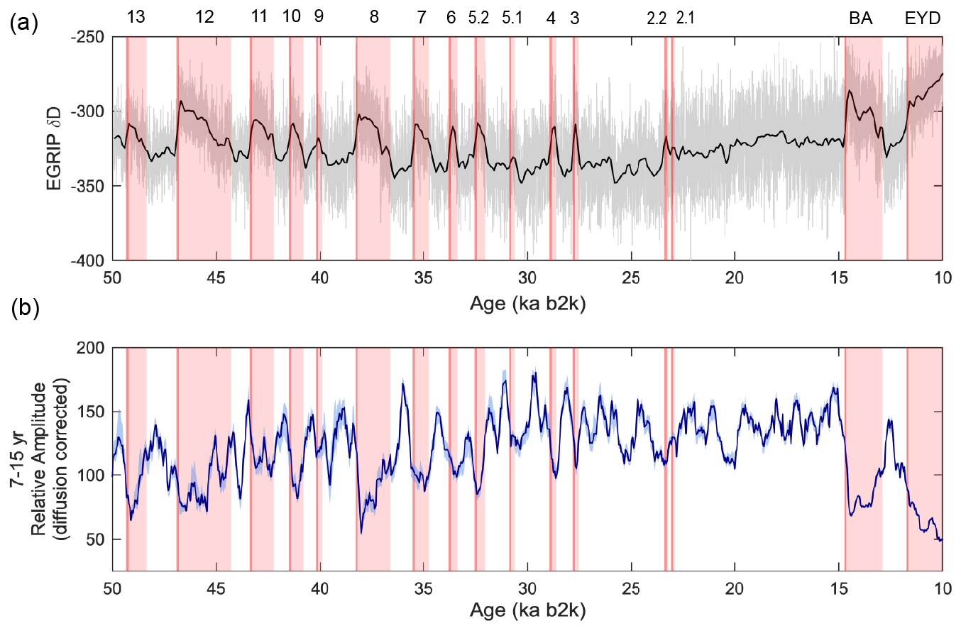
Figure 3 (a) EGRIP δD (black; window = 400 years; time step = 50 years) shaded by duration of warm Greenland Interstadial periods 2–13, the Bølling–Allerød (BA), and end Younger Dryas (EDY) (red; Rasmussen et al., 2014). (b) High-resolution analysis of the 7–15-year isotopic variability (dark blue; window = 400 years; time step = 50 years) with uncertainty bounds (light blue). D–O events are indicated on the upper x axis.

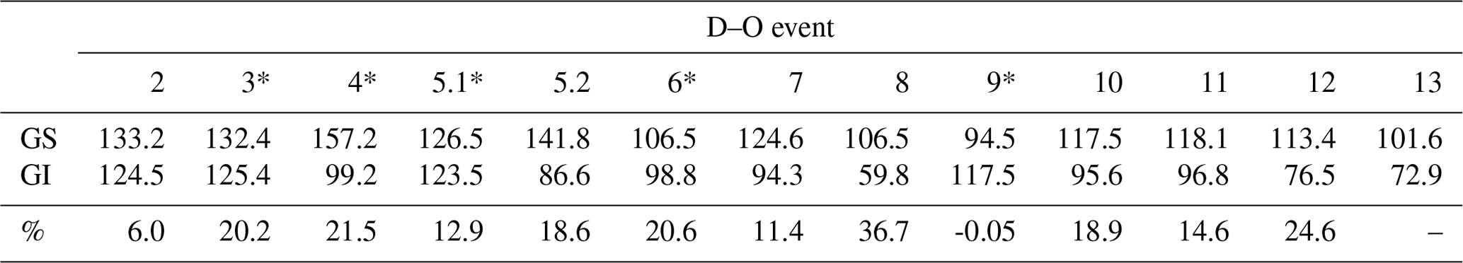
Table 1 Percent (%) reduction in the 7–15-year diffusion-corrected variability (‰² yr) between Greenland stadial (GS) onset and the following Greenland interstadial (GI). D–O events marked by an asterisk are characterized by interstadial phases shorter than the 400-year window size (240, 300, 240, 380, and 260 years for D–O events 3, 4, 5.1, 6, and 9, respectively). Due to the brief duration of GI 2.1 and 2.2 (collectively referred to as D–O 2 in Table 1), one 400-year window is placed at the onset of GI 2.2 (i.e., 23.34 ka b2k), which encompasses the entirety of GI 2.2, the majority of GI 2.1, and the short-lived stadial phase between each interstadial (Rasmussen et al., 2014).

3.2 HadCM3 model output

Interannual-scale (i.e., 7–15-year) temperature variability is assessed for northeastern Greenland and the broader North Atlantic region. We find that temperature variability and mean temperature at the EGRIP site are negatively correlated (i.e., colder states are characterized by greater fluctuations in atmospheric temperature, and vice versa) (Fig. 6b). These results agree well with our observations. To understand a wider regional context of temperature variability, we show a correlation map of the 7–15-year variability across the North Atlantic relative to the 7–15-year variability at the EGRIP field site (Fig. 5a). Figure 5a shows that the strongest remote correlation outside of Greenland exists in the North Atlantic subpolar gyre region, southwest of Iceland, and extends into the southernmost portion of the Norwegian seas. Oceanic regions north of Iceland and east of Greenland (i.e., central Nordic seas) show very low correlation (Fig. A6).

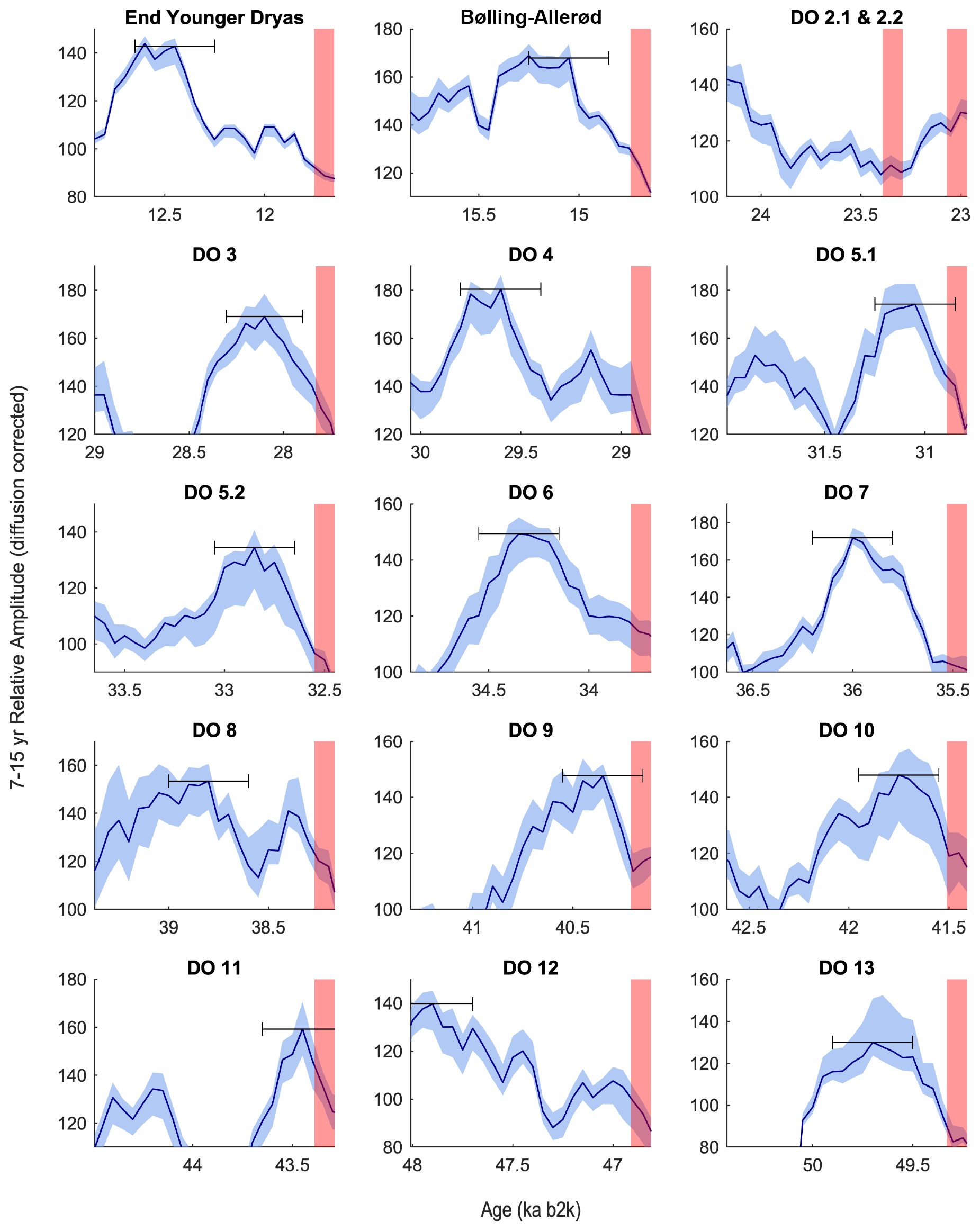
Figure 4 Magnified view of the GS–GI transitions from Fig. 3b for D–O events 2-13, the Bølling–Allerød (BA), and end Younger Dryas (EDY). High-resolution analysis of the 7–15-year isotopic variability (dark blue; window = 400 years; time step = 50 years) with uncertainty bounds (light blue). The horizontal black error bar indicates 400-year window range at the height of variability; red shading represents the 50-year buffer before and after onset of the GS–GI transition as defined in Rasmussen et al. (2014).

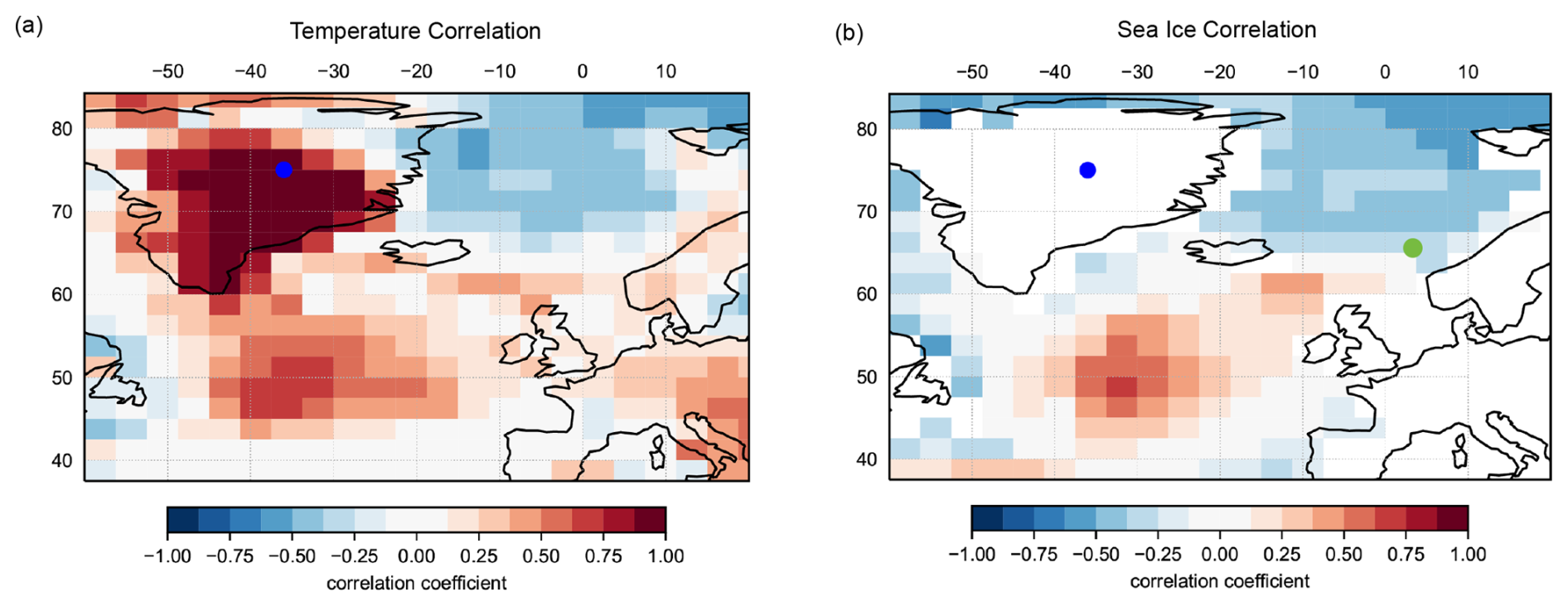
Figure 5 (a) Correlation between the 7–15-year temperature variability at EGRIP (blue dot) and other regional grid cells. (b) Correlation between the 7–15-year temperature variability at EGRIP (blue dot) and the 7–15-year sea ice variability for all regional oceanic grid cells. Red and blue shading depicts high and low correlations, respectively. The MD95-2010 core site is marked by a green circle.

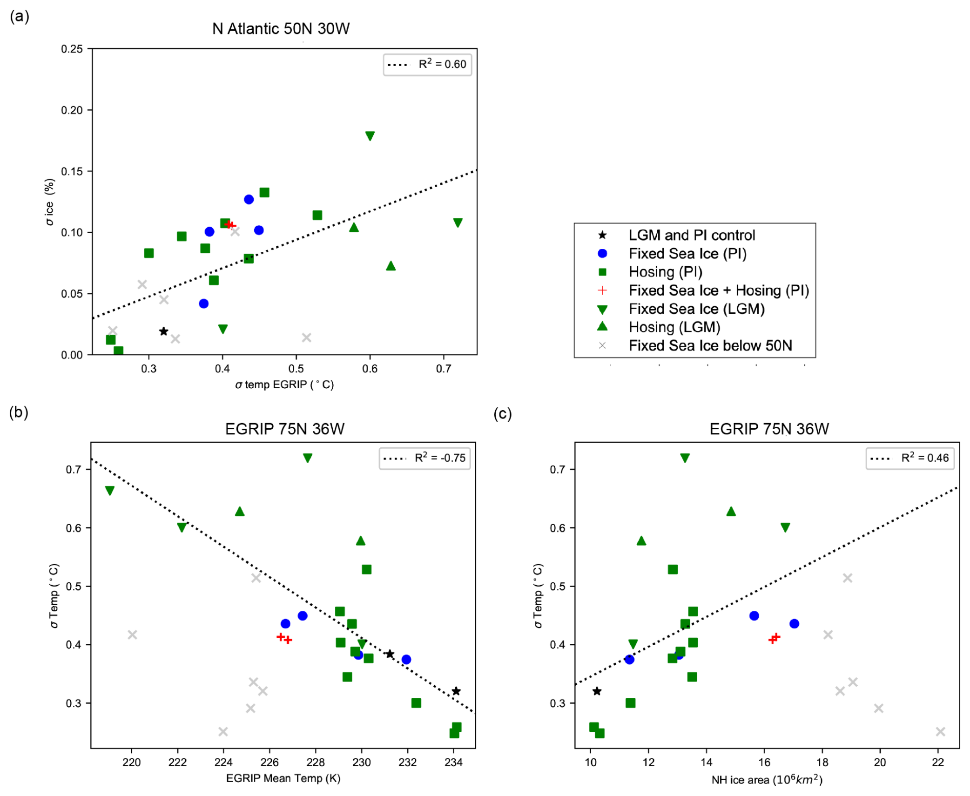
Figure 6 Individual model results for the (a) 7–15-year sea ice variability versus the 7–15-year EGRIP temperature variability near the high-correlation North Atlantic pocket (i.e., 50° N, 30° W). (b) The 7–15-year temperature variability versus mean temperature at the EGRIP location. (c) The 7–15-year temperature variability versus Northern Hemisphere ice area at the EGRIP location. Note that simulations including sea ice extending below 50° N (grey cross) have been excluded from the regression.

Next, we investigate the role of year-to-year sea ice fluctuations on climate variability over northeastern Greenland. Figure 5b displays the spatial correlation between the 7–15-year sea ice and temperature variability over northeastern Greenland. Again, the model output suggests ties between EGRIP and the North Atlantic, with the strongest correlations near 50° N, 30° W. Figure 6a shows the individual simulation results at 50° N, 30° W, with all simulations showing a trend of increased EGRIP temperature variability with increased sea ice variability. In the Nordic seas, simulations exhibit little to no correlation between interannual-scale sea ice fluctuations and temperature variability at EGRIP (Fig. A7). This finding is consistent with a persistent ice cover throughout the stadial and interstadial conditions (Li et al., 2010; Hoff et al., 2016; Sadatzki et al., 2020), where ice variability is inherently low.

Correlation does not demonstrate causation, so we examine other factors which might explain our results. Changes in sea ice variability might be associated with changes in mean temperature or with total sea ice area. Therefore, we compare the strength of these variables in explaining trends of high-frequency temperature variability at the EGRIP location. Figure 6b shows how the EGRIP temperature variability covaries with mean temperature. There is a strong negative correlation for all simulations, except those marked by grey crosses (Fig. 6b). This subset of simulations contains unrealistic sea ice prescriptions (i.e., sea ice extends south of 50° N) (Brennan et al., 2013; Dokken et al., 2013; Sadatzki et al., 2020). The extended sea ice cover causes a reduction in the temperature variability that is greater than the reduced mean temperature would suggest; the grey crosses sit well below the regression line. Similarly, Fig. 6c shows how the EGRIP temperature variance covaries with total North Atlantic sea ice area. We might expect that lower mean temperatures in Greenland are associated with extended sea ice cover, and it is therefore the mean sea ice cover that affects EGRIP temperature variability. As with mean temperature, we find that the unrealistic sea ice extent simulations fall far from the regression line. Furthermore, the correlation amongst realistic simulations is low (R²=0.45), relative to other comparisons. Thus, the mean temperature and sea ice extent alone cannot explain shifts in temperature variability across LGP climate states. By contrast, a comparison between the 7–15-year EGRIP temperature variability and North Atlantic sea ice variability exhibits a higher agreement (R²=0.60) for all simulations (i.e., both realistic and unrealistic prescriptions); grey crosses fall on or near the regression line (Fig. 6a). This indicates a robust relationship and, crucially, that the 7–15-year sea ice fluctuations in the North Atlantic are an excellent predictor of EGRIP temperature variability on similar scales.

4 Discussion

The results of this study are twofold. First, using HadCM3, we identify a critical coupling between interannual-scale North Atlantic sea ice fluctuations and high-frequency temperature variability over northeastern Greenland throughout the LGP. Conceptually, these results can be accounted for by our isotopic observations (i.e., stronger high-frequency variability during GS periods, and vice versa). Glacial stadial phases are characterized by lower average temperature and sea ice extending to the North Atlantic. It is possible that greater excursions in sea ice concentration were driven by the enhanced latitudinal range between maximum summer and winter ice extents (Sadatzki et al., 2020), which presumably changed on a year-to-year basis. These seasonal variations would impart volatility in high-frequency temperature fluctuations on annual, interannual, and decadal scales via ice–atmosphere feedbacks. By extension, Rayleigh distillation and the isotopic signature of precipitation at EGRIP would also be impacted.

An additional contribution to enhanced isotopic variability during stadial phases may stem from altered source-to-sink pathways. With large seasonal swings in the capping and exposure of the ocean surface by sea ice, evaporative sources upstream of EGRIP would also be altered. As a consequence, the variability in evaporative source signatures and temperature gradients of moisture transport to northeastern Greenland would increase. An isotope-enabled GCM is required to test this hypothesis.

Our second, and key, finding is that reductions in the 7–15-year isotopic variability generally begin hundreds of years prior to abrupt D–O warming at the EGRIP site. Taken together with results from HadCM3, we suggest that a fundamental change in North Atlantic sea ice dynamics occurs in the centuries leading to Greenland warming. One possibility is that the winter maximum ice extent retracted north of the high correlation North Atlantic pocket (50° N, 30° W) in the centuries leading to abrupt D–O warming, thereby reducing the latitudinal range between seasonal extents and overall mean ice extent. Based on our results from HadCM3, such a change would also be correlated with a lower 7–15-year temperature variability at the EGRIP. Alongside this, a more exposed ocean surface in winter may increase winter temperatures, ultimately increasing mean annual temperatures at EGRIP. Some GS phases (i.e., prior to D–O events 5.2, 8, and 10) exhibit a small rise in δD in the centuries prior to the abrupt temperature increase. It is possible that the GS phases which do not exhibit this behavior experience a muting of the δD increase due to source moisture deriving from more northerly and isotopically depleted water as the ice edge recedes.

The following section outlines a framework in which this hypothesis fits within the existing literature. It has been previously suggested that a salt oscillator in the North Atlantic drove bimodal shifts in the AMOC and, hence, transitions between stadial and interstadial conditions during the LGP (Broecker et al., 1990; Peltier and Vettoretti, 2014). Using HadCM3, Armstrong et al. (2022) demonstrates a complex ocean–atmosphere–ice feedback capable of maintaining a millennial-scale salt oscillation mechanism. To summarize, the salinity gradient between the tropics and North Atlantic regulates advection between these regions, thus governing the strength of the AMOC, northward heat transport, and related regional climate effects. In the model, the onset of cold stadial periods are marked by a sluggish AMOC, accumulating salinity in the tropics, and diminishing salinity in the North Atlantic. Due to a reduction in the transport of dense (i.e., salty) and warm water to the north, deep-water formation drops to a minimum. Concurrently, the difference in PSUs (i.e., practical salinity units) between the tropics and North Atlantic approaches a maximum. It is precisely this feature, peak salinity gradient, that kick-starts the AMOC and initiates a transition from the stadial to interstadial in the salt oscillator framework.

Sea ice and surface freshwater fluxes are deemed critical in developing the salinity gradient, though their effects are spatially heterogeneous. In the North Atlantic, both stadial and interstadial periods are characterized by a freshening effect. Winter ice traps freshwater by freezing seawater and trapping overhead precipitation. The summer melt season flushes out both freshwater sources, resulting in a net freshening effect. Due to the reduced ice extent during interstadials, this freshening effect is dampened. A relevant detail of the salt oscillation mechanism is that North Atlantic salinity and the AMOC strength begin to steadily increase partway through the stadial phase (i.e., centuries prior to interstadial onset), priming the system for an abrupt shift. Critically, Armstrong et al. (2022) proposes reduced regional freshening due to gradual sea ice retreat as a likely cause. Our study provides paleoclimate and modeling evidence in favor of this suggestion.

A useful tool in corroborating the centennial-scale phase offset is empirical evidence of North Atlantic sea ice behavior with similar lead–lag behavior. Unfortunately, high-resolution records are sparse. One such analysis (Sadatzki et al., 2020) finds that declining seasonal sea ice in the lower-latitude Norwegian Sea (MD99-2284; 62° N, 0° W) initiated ice-free conditions further north (MD95-2010; 66° N, 04° E) prior to the Greenland temperature increase. In this study, sediment core age models are tied to GICC05 using a stratigraphic alignment of ARM (anhysteretic remanent magnetization), near-surface temperature, and cryptotephra layers with NGRIP δ¹⁸O. At the northern core site, a change in the properties of the biomarkers brassicasterol and HBI III, occurring in open-ocean environments, is detectable centuries prior to the abrupt GS–GI transition. A direct comparison to our isotope variability time series shows near-simultaneous shifts, possibly indicating a common link (Fig. 7). However, the MD95-2010 sediment core site falls just outside the high-correlation pocket suggested by HadCM3. One explanation is that the large-scale changes in Norwegian Sea mean ice extent are not associated with shifts in variability, unlike the North Atlantic. It is also possible that the model grid cells are too coarse to resolve fine detail in the Norwegian Sea ice movement, thus failing to detect shifts in the variability as the mean sea ice area changes. Nevertheless, this realization prompts interest in high-resolution sea ice proxy records at the heart of the high-variance correlation.

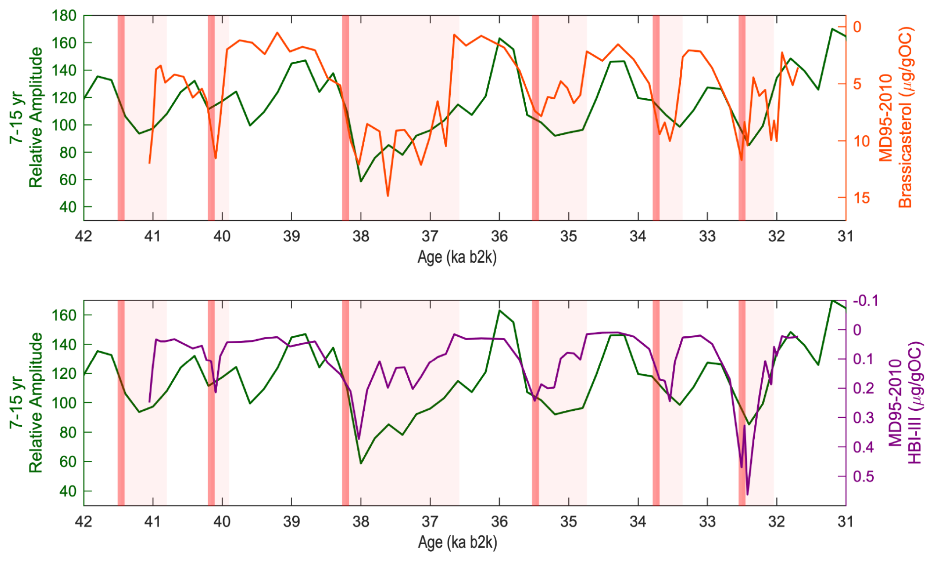
Figure 7 Comparison between the 7–15-year diffusion-corrected isotopic variability at the EGRIP and open-ocean biomarkers (i.e., HBI III and brassicasterol) recovered from ocean sediment at 66° N, 04° E. Dark red shading represents the 50-year buffer before and after the onset of GS–GI transition. Light red shading represents the duration of the GI period, as defined in Rasmussen et al. (2014).

Last, an inexplicable component of this study is the continuation of large excursions in high-frequency isotopic variability, even when the D–O cycling is turned off for long stretches (i.e., 27–15 ka b2k). In some cases, the fluctuations are comparable in magnitude to those occurring across prior GS–GI transitions. It seems that a climate variability oscillation is inherent to the LGP background state, yet it does not result in an abrupt mean climate change (i.e., D–O events) based on certain boundary conditions which remain to be seen. Due to the simultaneous occurrence of the Last Glacial Maximum during this time frame, an obvious factor to test in future studies is the height and extent of the Laurentide and Scandinavian ice sheets and their effects on climate variability.

There are additional explanations for the lead–lag result, though they currently lack strong evidence. The first variable to consider is stratigraphic noise, which is a non-climatic variability imparted to the water isotope record due to processes like precipitation intermittency, surface sublimation, and wind-driven snow erosion (Fisher et al., 1985; Helsen et al., 2005; Town et al., 2008; Zuhr et al., 2021). Stratigraphic noise hinders the extraction of climate-induced high-frequency signals during low-accumulation phases (e.g., LGP stadials), thus raising concerns that local depositional processes may also drive the results presented in this study. Unfortunately, the temporal evolution of stratigraphic noise cannot be quantified directly, and currently, there are no LGP signal-to-noise ratio comparisons with nearby Greenland ice cores. Still, contributions of non-climatic noise are likely state-dependent (e.g., GI vs. GS phases) and inherently linked to accumulation rate. The EGRIP 7–15-year variability also exhibits a centennial lead–lag with accumulation, suggesting that the primary driver for this deviation lies elsewhere (Fig. A8).

Second, water isotope diffusion is a property not exclusively set at the ice sheet surface, but one that reflects the duration of the firn densification process. If the surface climate changes, this impacts concurrent precipitation in addition to the firn column below via temperature gradients, which are important for grain metamorphosis and vapor movements via overburden pressure and barometric pumping. Changes in the interannual-to-decadal variability in ice that is deeper (i.e., older) than the abrupt D–O warmings may be driven by shifting thermal gradients that affect grain metamorphosis and vapor transport in such a way to keep pore pathways open longer, thereby enhancing gas mixing and ultimately reducing the water isotope variability in older ice. Such a mechanism is not currently captured in accepted firn models (e.g., Johnsen et al., 2000).

As an analysis of the shifting thermal gradients based on results from the West Antarctic Ice Sheet (WAIS) Divide Ice Core in West Antarctica, the diffusion lengths (Jones et al., 2017b) and total air content (TAC) (Buizert et al., 2021) exhibit anomalous increases around 19 ka b2k as temperatures rose during deglaciation. TAC may reflect thermal gradients, overburden pressure, or barometric pumping but may also be sensitive to surface climate drivers. Efforts to model the anomalous WAIS Divide period have mostly been unsuccessful (Jones et al., 2017b). The increase in diffusion at the WAIS Divide was not accompanied by any reductions in the interannual-to-decadal isotopic variability (Jones et al., 2018), which dramatically lowered 3000 years later when diffusion lengths and TAC decreased, which is the exact opposite of what might be expected based on the above explanation. There are further complicating factors with a thermal gradient–firn metamorphosis hypothesis. Figure A9 shows that the multi-decadal variability (20–30 years) in the EGRIP water-isotopes – frequencies that should have nearly zero impact from firn diffusion – also exhibit a centennial-scale lead time in line with the higher frequency and more diffused 7–15-year band. This suggests that (1) firn processes that affect diffusion, like thermal gradients, cannot be a driving factor because the entire spectrum of variability (both diffused and non-diffused frequencies) is altered or (2) our current physical understanding of diffusion is substantially wrong and highly non-Fickian. Furthermore, there are large changes in the interannual-to-multi-decadal variability between 27–15 ka b2k (up to 40 % reductions) when DO cycles are infrequent, and hence, no dramatic thermal shifts are imparted to the firn column.

As a final note, evidence of centennial-scale lead times in sea ice proxies from Norwegian sediment cores as compared to Greenland abrupt warming, as well as the model evidence presented here, suggest the weight of evidence is currently in favor of a regional climate driver rather than firn dynamics or stratigraphic noise. However, if new evidence arises in the future (e.g., improved firn modeling or signal-to-noise ratio analysis across multiple deep Greenland ice cores) our working hypothesis will need to be modified.

5 Conclusions

Interannual variability and decadal variability are important aspects of paleoclimate reconstructions and assessments of D–O warming, but such records have been previously sampled at a lower resolution, which may exclude important climate insights that are documented here. In this study, the millimeter-scale EGRIP water isotope record is used to quantify the diffusion-corrected 7–15-year isotopic variability for northeastern Greenland to 49.9 ka b2k. Importantly, we provide evidence that high-frequency LGP Greenland climate variability became decoupled from local mean temperature in the centuries preceding D–O warming. Our initial model analysis suggests that lower-latitude feedbacks associated with interannual North Atlantic sea ice change may be a driver of this offset. As the cause of D–O cycles continues to be debated, these results should be considered.

Additionally, future isotope-enabled GCM studies may benefit from utilizing the high-frequency EGRIP variability time series, presented here, to constrain boundary conditions or benchmark model output. We suggest targeted tests aimed at temporally reconciling the centennial-scale offset with sea ice behavior to better understand the regional North Atlantic climate change within the context of abrupt D–O warming. Analysis of high-resolution sediment proxy records from critical locations identified in this study may also clarify uncertainties.

Appendix A

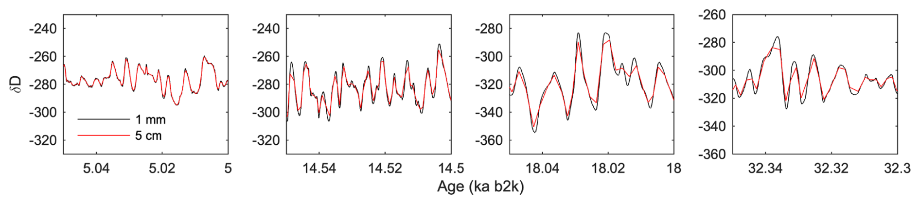
Figure A1 Comparison of original 1 mm EGRIP δD (black) to downsampled 5 cm EGRIP δD (red). Each window contains 50 years of data with progressively older windows towards the right. A lower sampling resolution artificially reduces the amplitude of interannual and decadal fluctuations after approximately 12 ka b2k.

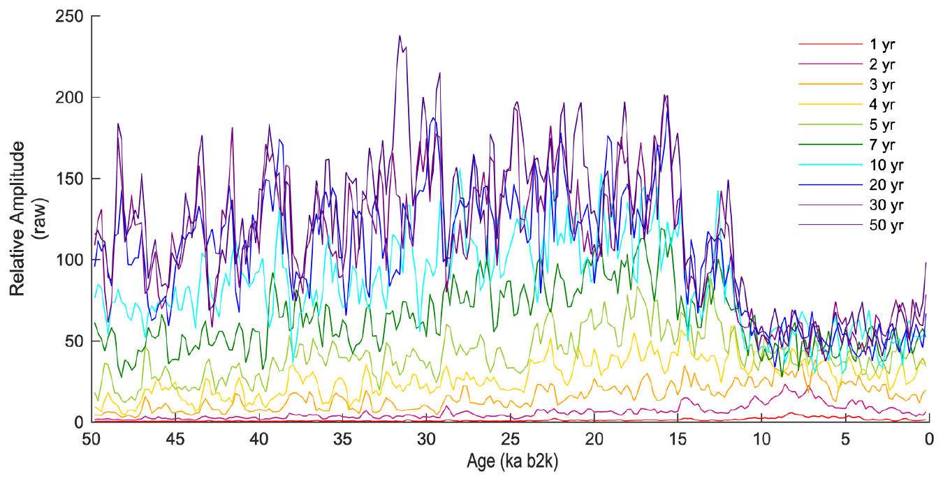
Figure A2 Strength of raw (i.e., non-diffusion-corrected) and isolated frequencies in the EGRIP δD record. Substantial attenuation with age due to diffusion in the firn layer is evident in the 1–5-year signals.

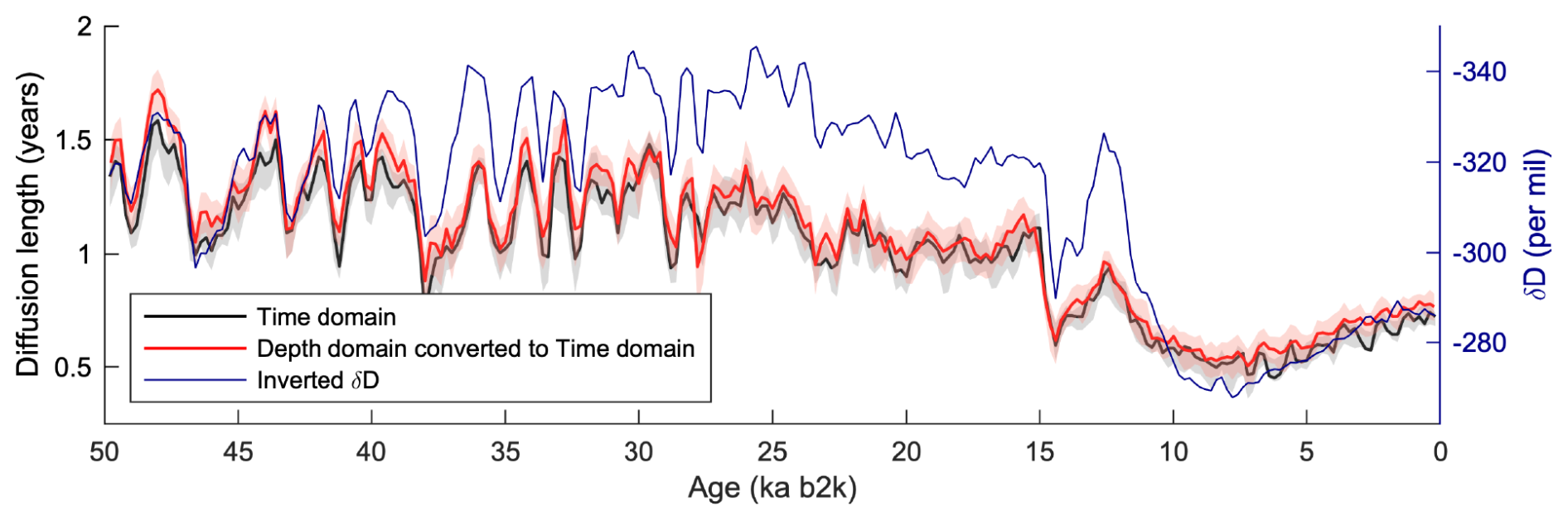
Figure A3 Comparison of diffusion lengths calculated using the EGRIP δD record in the time domain (black) versus the depth domain converted to the time domain using annual layer thickness (red). Uncertainties largely overlap with some deviations prior to 43 ka b2k. The inverted EGRIP δD (blue) is plotted to show the synchronous shifts in the diffusion length with the mean climate state.

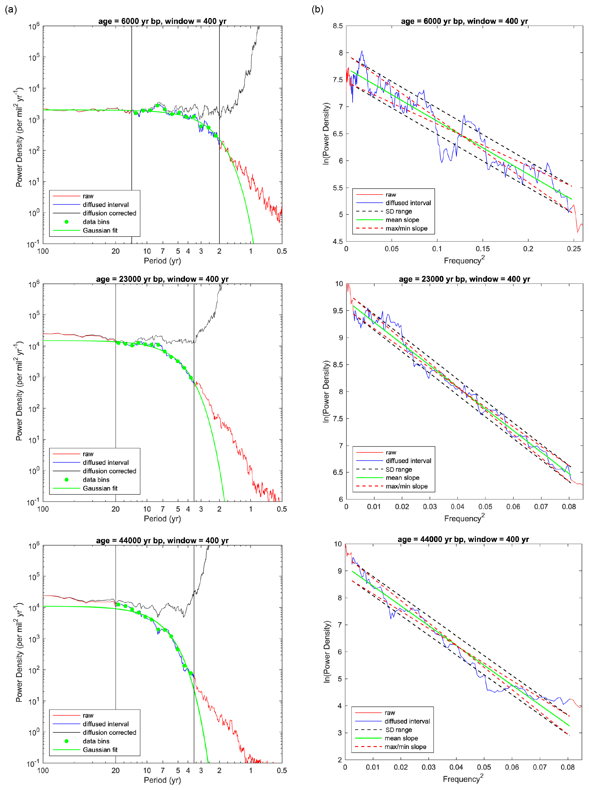
Figure A4 (a) Examples of 400-year power density spectra (PDS) fitted by Gaussian regression for diffusion correction (progressively older windows towards the bottom of the panel). There are 12 equally spaced logarithmic bins used in the fitting so that higher frequencies with an increased data density do not skew the correction. (b) Examples of an uncertainty calculation. The maximum and minimum slopes of [ln(PDS) versus frequency²] within 1 standard deviation represent the high- and low-uncertainty bounds, respectively.

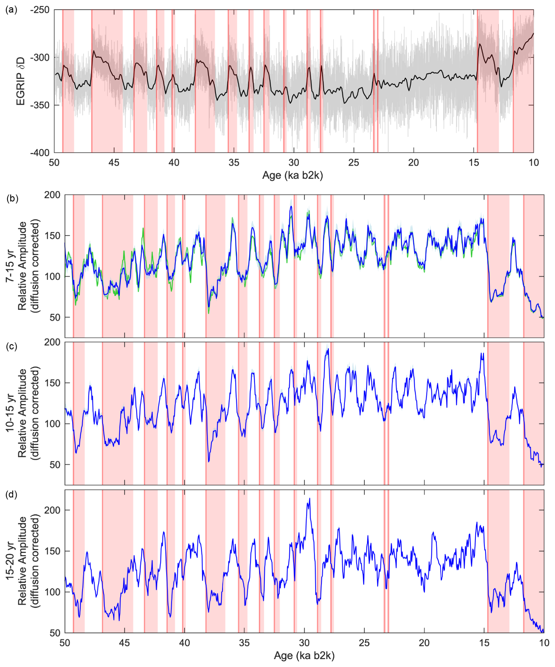
Figure A5 (a) The EGRIP δD (black; window = 400 years; time step = 50 years) shaded by the duration of warm Greenland interstadial periods 2–13, the Bølling–Allerød, and the Holocene (red; Rasmussen et al., 2014). High-resolution analysis of the (b) 7–15-, (c) 10–15-, and (d) 15–20-year EGRIP isotopic variability (blue; window = 400 years; time step = 50 years) using diffusion lengths which have been calculated in the depth domain and converted to the time domain using annual layer thickness. Results from Fig. 3 (green) are plotted underneath the results in panel (b) to demonstrate that the method of the diffusion length calculation does not affect the lead–lag relationship between the variability and the mean.

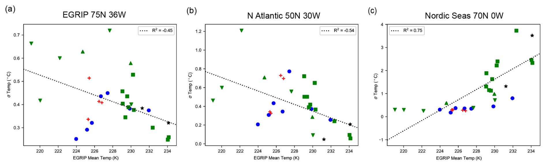
Figure A6 Individual simulation results for the correlation between the 7–15-year temperature variability and the EGRIP mean temperature at the (a) EGRIP, (b) North Atlantic, and (c) central Nordic seas.

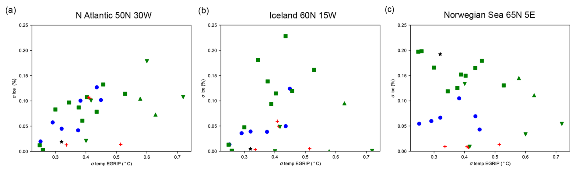
Figure A7 Individual simulation results for the correlation between the 7–15-year sea ice variability and the 7–15-year EGRIP temperature variability in (a) the North Atlantic, (b) Iceland, and (c) the Norwegian Sea.

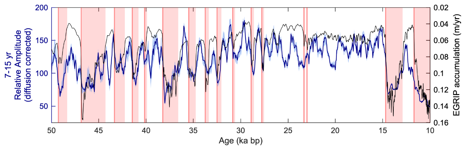
Figure A8 Coevolution of the high-resolution 7–15-year isotopic variability (dark blue; window = 400 years; time step = 50 years) with an inverted EGRIP accumulation (black).

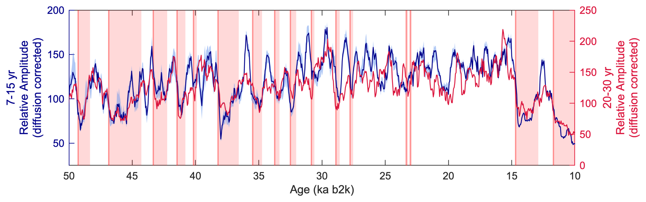
Figure A9 Coevolution of the EGRIP high-resolution 7–15- (dark blue; window = 400 years; time step = 50 years) and 20–30-year isotopic variability (red; window = 400 years; time step = 50 years).