Total air content measurements from the RECAP ice core

In this paper, total air content (TAC) of the Renland Ice Cap Project (RECAP) core, drilled in summer 2015, is presented. In principle, TAC is a proxy for the elevation at which the ice was originally formed, as the TAC in ice cores is predominantly influenced by surface air pressure and conditions like temperature and local summer insolation. This, however, presupposes dry sintering of the firn with no surface melting. The RECAP TAC data show incoherently low values in the Holocene Climate Optimum (6 to 9 kyr b2k) and in part of the last interglacial (119 to 121 kyr b2k) originating from melt layers that render the TAC data unfit for paleo-elevation interpretation. Melt instances can, however, be used to reconstruct summer temperatures, and we find that Renland was ∼ 2 to 3 °C warmer compared to today in the early Holocene. Similarly, samples from the previous interglacial hint at summer temperatures that were at least 5 °C warmer than today.

The glacial section (11.7 to 119 kyr b2K) has consistent TAC values, which in principle facilitate the past elevation calculations. However, we observe TAC variations related to Dansgaard–Oeschger events (D-O) that cannot originate from elevation changes but must be linked to changes in the firn structure. We analyse the pattern of these structural changes in the RECAP and NGRIP cores and conclude that only samples from the stable portion of the Last Glacial Maximum are suitable for elevation reconstructions. Within uncertainty, the elevation was similar to today at the last glacial maximum.

1 Introduction

We present the first total air content (TAC) record from the Renland ice cap from the RECAP core drilled in 2015.

The motivation for studying TAC in the Renland ice core was that Vinther et al. (2009) used the first Renland ice core (Johnsen et al., 1992) as an anchor point in their reconstruction of the Holocene Greenland Ice Sheet (GIS) history. They argued that the ice cap has not experienced significant ice flow or elevation changes due to its isolation from the GIS owing to the surrounding topography. The TAC signal from the RECAP core could be used to infer the elevation changes, thereby supporting or refuting their assumption. However, in the course of the study we learned that the RECAP TAC is affected by melt during the Holocene, making it impossible to use it for elevation reconstructions. On the other hand, the melt fractions in the samples construed by assuming a linear relationship between the TAC and melt fraction of a sample allow for estimating summer temperatures. We apply this concept to samples from the previous interglacial. The effect of local summer insolation on the RECAP TAC signal is analysed. The RECAP TAC signal from the glacial section is unaffected by melt but is affected by rapid climate change events that hinder reconstruction of the past elevation of the Renland ice cap, with the exception of the climatically stable phase of the Last Glacial Maximum (LGM).

1.1 The RECAP ice core

The Renland ice cap is situated in eastern Greenland on a high-elevation plateau on the Renland Peninsula in the Ittoqqortoormiit (Scoresbysund) fjord (Fig. 1) and has a present elevation of 2340 m a.s.l. at the summit. The RECAP core is ∼ 584 m long and was drilled to bedrock in 2015 at an elevation of 2315 m a.s.l. (71°18^′18^′′ N, 26°43^′24^′′ W) near the summit, about 1.5 km away from the 1988 drill site (Johnsen et al., 1992). The present-day annual mean temperature is −17.8 °C measured at 20 m depth in the firn, and the present accumulation rate is approximately 0.5 m of ice-equivalent precipitation per year. In the interior of the GIS the average size of the air bubbles monotonically decreases with depth until they disappear and form clathrates (Shoji and Langway, 1982). The enclosed air in the RECAP core exists fully in the form of air bubbles. At the given temperature, clathrate formation would start below the bedrock depth of ∼ 584 m below surface (Uchida and Hondoh, 2000). The bubble diameter, however, is increasing again from about 530 m below the surface (Supplement Fig. S3). This may be due to rapid thinning of the annual layers in the Renland ice cap causing the small bubbles to coalesce to form bigger bubbles.

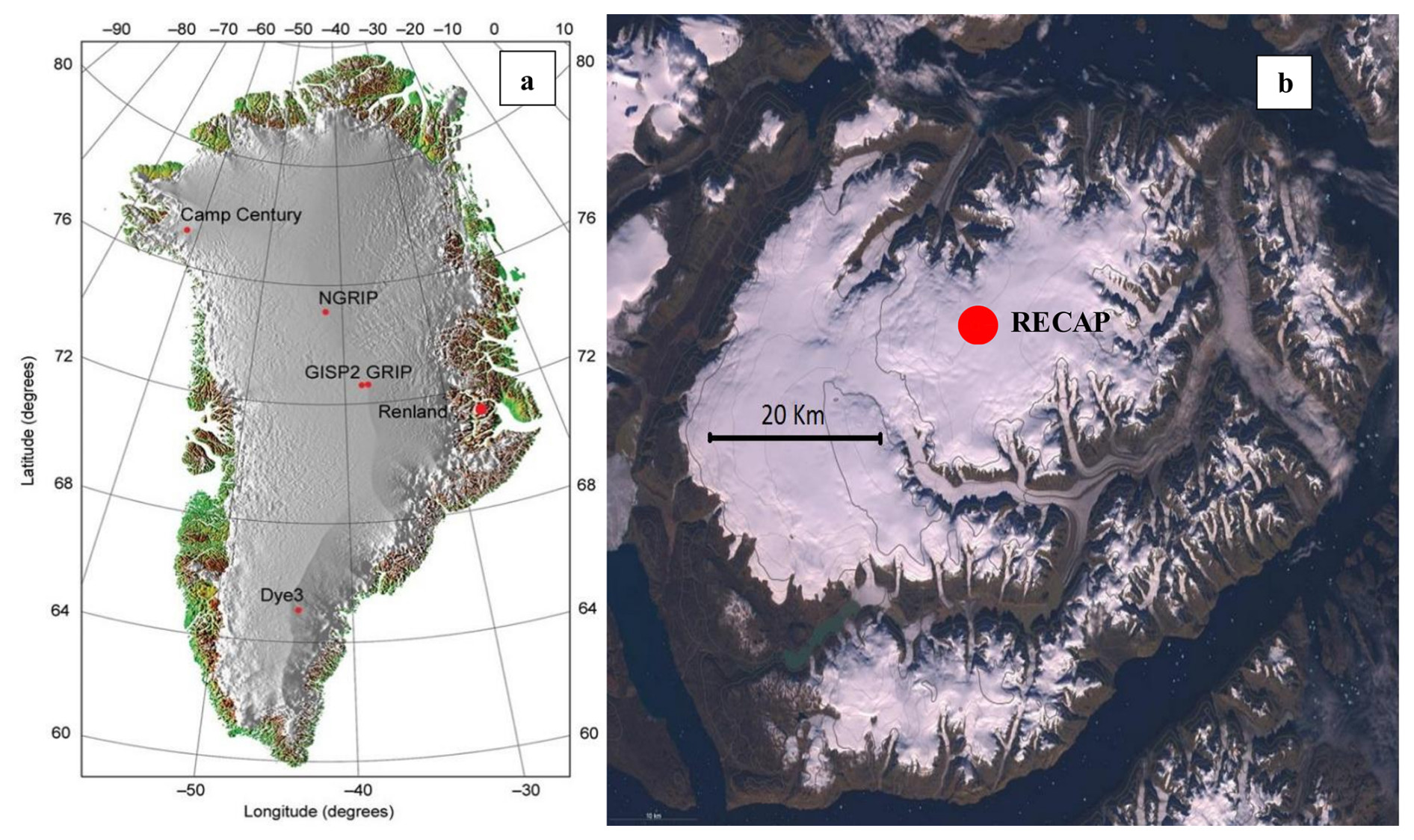
Figure 1 (a) Map of Greenland showing the location of the Renland ice cap and other cores (Danish Cadastre). (b) Satellite image of the Renland Peninsula, which is almost entirely covered by the Renland ice cap (Landsat).

1.2 Total air content in ice

1.2.1 Principle

The density of dry sintered snow at the surface of an ice sheet is typically 0.3–0.35 g cm⁻³. This open porous firn is then densified by compaction and dry sintering to a density of 0.81–0.84 g cm⁻³ where the open pores are isolated. The amount of gas trapped at this time, the total air content (TAC), depends on the pore volume, the temperature, and the pressure (e.g. Martinerie et al., 1992). It is usually expressed as cubic centimetres of gas per kilogram of ice at standard temperature and pressure (STP) (Eq. 1), where V_c, P_c, and T_c are pore volume per kilogram of ice, pressure at close-off, and temperature at close-off, respectively. P and T are standard temperature and standard pressure (1013 mbar and 273.15 K).

$$\begin{array}{}\text{(1)}& \mathrm{TAC}=V_{\mathrm{c}}{\displaystyle \frac{P_{\mathrm{c}}}{T_{\mathrm{c}}}}{\displaystyle \frac{T}{\mathrm{P}}}\end{array}$$

With known V_c and T_c, elevation changes can be obtained applying the barometric formula (Eq. 2):

$$\begin{array}{}\text{(2)}& P_{\mathrm{c}}=P_{\mathrm{a}}{\left[{\displaystyle \frac{T_{\mathrm{a}}}{T_{\mathrm{c}}}}\right]}^{\frac{g{M}_{\mathrm{air}}}{R\left(\frac{\mathrm{d}T}{\mathrm{d}z}\right)}}\mathrm{with}{T}_{\mathrm{c}}=T_{\mathrm{a}}+{\displaystyle \frac{\mathrm{d}T}{\mathrm{d}z}}\left(h_{\mathrm{c}}-h_{\mathrm{a}}\right),\end{array}$$

where P_c is the pressure at altitude h_c, while P_a, T_a, and h_a are pressure, temperature, and elevation at sea level, respectively. $\mathrm{d}T/\mathrm{d}z$ is the lapse rate at the location, M_air the molecular mass of air, g the gravitational constant, and R the gas constant. A 1 % change in TAC at the elevation of RECAP corresponds to a pressure change of about 7 mbar and 80 m change in elevation.

It has been observed that the pore volume (V_c) at the air isolation depth exhibits a slight dependence on temperature (Martinerie et al., 1994). This relationship can be described by the following linear equation, which has a correlation coefficient of 0.90:

$$\begin{array}{}\text{(3)}& V_{\mathrm{c}}\left({\mathrm{cm}}^{\mathrm{3}}{\mathrm{g}}^{-\mathrm{1}}\right)=\mathrm{6.95}\times {\mathrm{10}}^{-\mathrm{4}}{T}_{\mathrm{c}}\left(\mathrm{K}\right)-\mathrm{0.043}.\end{array}$$

We will apply this parameterisation based on data from sites with a temperature range ∼ −15 to −60 °C to calculate the pore volume for the RECAP core.

At any site, short-term sub-annual variability of V_c on the order of 20 % is observed. It is explained by the variability of the density originating from summer to winter precipitation and successive metamorphosis throughout the firn column to the air insolation depth (Hörhold et al., 2011). In addition, high-density wind crusts potentially add to the variability (Martinerie et al., 1994).

1.2.2 TAC variations at orbital scale

It has been discovered that both O₂ $/$ N₂ ratios and TAC anticorrelate with local summer insolation in Greenland and Antarctica (Suwa and Bender, 2008; Kawamura et al., 2007; Raynaud et al., 2007, and references therein). The reasoning brought forward is that summertime insolation influences the metamorphism of snow near the surface of polar ice as it causes evaporation and grain growth (Bender, 2002). The explanation given for this is that summer insolation causes rapid grain growth in the snow surface by creating an apparent summer temperature gradient. Thus, the increase in grain size below the surface affects the densification process. An increase in insolation thereby causes the grain size to increase, porosity at close-off to decrease, and density at close-off to increase. The proposed mechanism explains the anticorrelation between the integrated summer insolation and the TAC. As insolation increases, porosity at close-off and pore volume decreases, causing an overall decrease in the TAC. The O₂ $/$ N₂ signal results from fractionation at the close-off as a consequence of mentioned surface metamorphism processes (Suwa and Bender, 2008). Both TAC and O₂ $/$ N₂ have proven to be reliable proxies for local insolation and hence can be used for orbital dating of ice cores despite the remaining gaps in our understanding of the physical mechanisms (Lipenkov et al., 2011). After correcting for the effect of changing local solar insolation, TAC can be interpreted to give paleo-surface elevations, with high TAC corresponding to lower elevations (Raynaud et al., 1997; Raynaud et al., 2007; NEEM Community Members, 2013).

1.2.3 Perennial TAC variations

TAC has also been found to be influenced by rapid climatic transitions in connection with Dansgaard–Oeschger (D-O) events during the last glacial in the Greenlandic NGRIP core (Eicher et al., 2016). We expect to see similar effects for the RECAP core. Surprisingly, this also seems to be the case for some Antarctic sites (Epifanio et al., 2023). Lacking understanding for those rapid TAC variations it seems that only TAC measurements from climatically stable periods should be used for past elevation estimation.

2 Measurements

Measurements of the RECAP ice core were made at PICE (Physics of Ice, Climate and Earth) and PSU (Penn State University). While the system at PICE is dedicated to TAC measurements following the barometric method and giving absolute calibrated volumes (Lipenkov et al., 1995), the measurements at PSU are a byproduct of measurements for δ¹⁵N and CH₄ contents.

At PICE, air is extracted from cubical samples of 10 to 15 g of ice by two melt–refreeze cycles under vacuum. The extracted air is passed through a dry ice and ethanol water trap and quantitatively trapped on HayeSep at LN₂ temperature. The air is then expanded into a calibrated measuring volume by warming up the HayeSep D trap. Experimental details are given in Supplement Sect. S1. Data from measurements at PICE are published in Blunier (2024).

Two sets of TAC measurements are obtained at PSU. The samples used for CH₄ measurements are cylinders with a diameter of 4.1 cm, height of 5.5±0.3 cm, and weight of 65±3 g each, and the samples used in δ¹⁵N measurements are rectangular cubes of ice ($\mathrm{2}\times \mathrm{1.2}\times \mathrm{5}$ cm) weighing ∼ 13 g each. In both of these measurements, an automatic air extraction device (referred to as “The Spider”) that employs the vacuum volumetric principle is used. The volume of the extracted air is measured, and the air samples are then used for CH₄ and δ¹⁵N measurements (Fegyveresi, 2015).

The Spider apparatus consists of 14 steel vessels used to hold ice samples, each with a total sampling volume of ∼ 96±2 cm³ (Fegyveresi, 2015). During measurements, the system performs a single melt–refreeze cycle to free the trapped air from within the ice (Fegyveresi, 2015). Ice samples are placed in the respective vessels and isolated from the ambient atmosphere using copper gaskets. The entire system is then evacuated to 0.3 mbar to remove air in each vessel's headspace, and various leak checks are performed to ensure the seals are intact with no contamination from ambient air. The ice samples are then melted, allowing the air trapped in the ice samples to escape into the headspace of the enclosing vessels. The melt is then refrozen, leaving the liberated air separated above each of the refrozen samples. Once the temperature of the ice reaches −69 °C, the air in each vessel is expanded into a vacuum manifold containing a 10 cm³ sample loop, which is then connected to a gas chromatograph (Fegyveresi, 2015). The pressure in the vacuum manifold with the ice core air sample is noted (generally between 60 and 80 Torr, corresponding to 80 to 107 mbar) before the loop is switched for CH₄ concentration or δ¹⁵N measurements. Solubility correction in connection with the CH₄ measurements is quite large (∼ 6 %) in this method due to the high ratio of sample to vessel volume, which yields a high headspace pressure that contributes to more gas getting stuck in the refrozen ice (Fegyveresi, 2015). The calibrations (volume and temperature) are given in Sect. S2. Data from PSU-δ¹⁵N measurements are published in Sowers (2018).

3 Cut bubble correction

Air bubbles at the surface of the sample are cut during sample preparation, resulting in air loss. Therefore, TAC measurements need to be corrected for the so-called “cut bubble effect” (CBE). The CBE correction approximates to 10 % near the close-off depth and decreases to around 1 % in deeper strata (Martinerie et al., 1990). Martinerie et al. (1990) derived the formula for the CBE assuming spherical bubbles:

$$\begin{array}{}\text{(4)}& \mathrm{TAC}={\left(\mathrm{1}-{\displaystyle \frac{\mathrm{1}}{\mathrm{2}}}\langle D\rangle {\displaystyle \frac{A_{\mathrm{S}}}{V_{\mathrm{S}}}}\right)}^{-\mathrm{1}}\cdot {\mathrm{TAC}}_{\mathrm{raw}},\end{array}$$

where D is the average bubble diameter in the sample, while A_S and V_S are the sample surface area and volume, respectively. In the current study, only samples analysed at PICE had their bubble diameters measured. A photograph of each sample is taken (Fig. S4) from which the average of 20 bubble diameters is taken as the sample bubble diameter. The average bubble diameter of every sample and the corresponding CBE calculations are provided in Sect. S3. TAC data from PSU are a byproduct of methane concentration and δ¹⁵N measurements. Bubble diameters have not been measured for these samples. In this study, we estimate the CBE for the PSU data from the PICE data. Bubble diameter decreases with depth through the Holocene section of the RECAP core. This is expected as the bubbles are compressed by the increasing pressure of the overlaying ice. Therefore, down to the Younger Dryas–Preboreal transition at 532.6 m below surface we calculate the CBE for the PSU data from the linear regression in the PICE data (120–530 m). For samples below 532.6 m we use the corresponding average of bubble diameters in the PICE data.

4 Comparison of datasets

The sample sizes, extraction devices, and measurement procedures are different at PICE and PSU. Correlation plots of the final data including all corrections from PSU are made to analyse their deviations from the TAC data obtained from the barometric method at PICE (Sect. S4). The datasets show a good correlation with the vacuum volumetric data obtained at PICE. However, between individual data points differences can be significant and result from an up to 1 m depth difference to the closest correspondent and rapid fluctuations in TAC. After applying all corrections, the pooled standard deviations of TAC for PICE, PSU-CH₄, and PSU-δ¹⁵N are 6.67, 6.80, and 6.11 cm³ kg⁻¹, respectively, excluding samples with obvious melt features. We observe no significant difference in the dispersion in the three datasets.

5 Results and discussion

The TAC data are presented on the RECAP GICC05 ice age timescale (Simonsen et al., 2019, and Sect. S5) in Fig. 2. The Holocene section of the record from 12 kyr b2k (section a) shows a decrease in TAC to roughly 80 cm³ kg⁻¹, and this is followed by an increase to present-day values. The variations in that section are caused by melt layers, as we will argue below. Similarly, section c, which is part of the previous interglacial period, is heavily affected by melt, with TAC as low as 20 cm³ kg⁻¹. In the first few metres of the record (section a) TAC is heavily affected by visible melt layers, with TAC being as low as 20 cm³ kg⁻¹. Based on the melt fraction, we will in the following reconstruct summer temperatures. The cold glacial section at 115–12 kyr b2k (section b) shows no signs of melt layers. However, rapid variations occur that seem related to rapid climate changes, as we will discuss below.

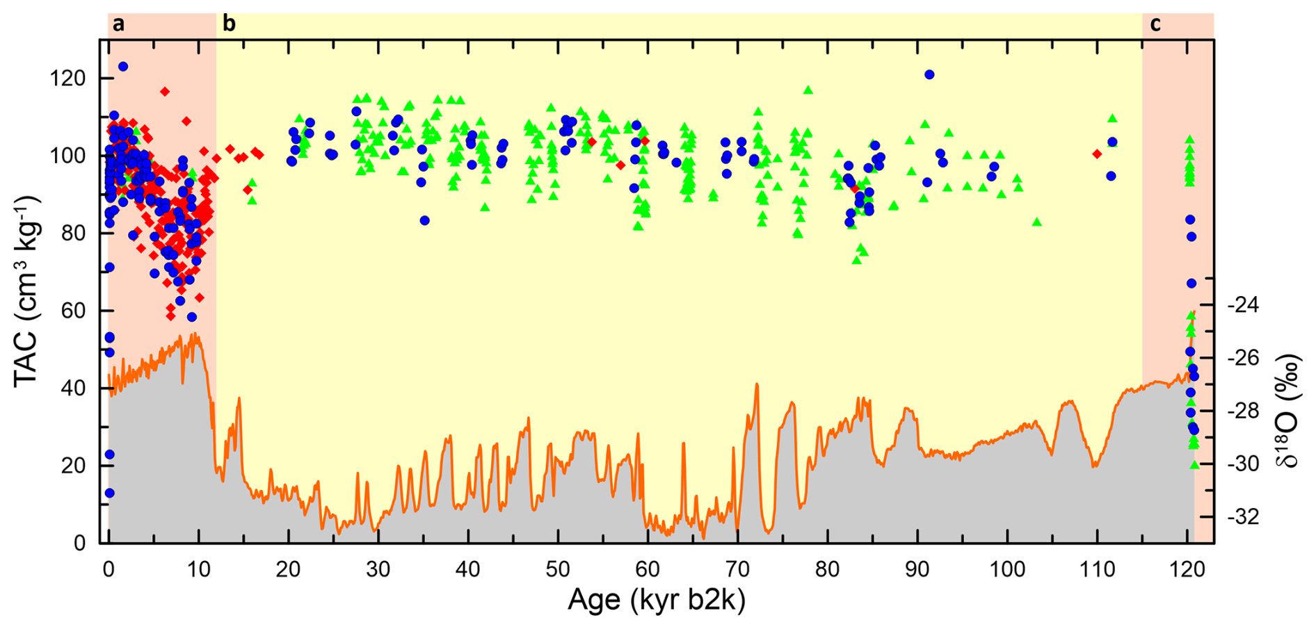
Figure 2 TAC and δ¹⁸O of the RECAP ice core, with sections a and c being affected by melt (peach) and section b unaffected by melt (light yellow). The top of the figure shows TAC from PICE, PSU-CH₄, and PSU-δ¹⁵N as blue dots, red diamonds, and green triangles, respectively. The bottom of the figure shows RECAP δ¹⁸O (red line) (Gkinis et al., 2024). The data are presented on the RECAP GICC05 ice timescale b2k (before 2000 CE). Note that samples with very low TAC around 110 yr b2k were deliberately picked because they show signs of melt.

5.1 The RECAP TAC Holocene record

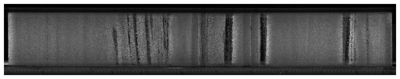
As outlined in Vinther et al. (2009), it is expected that the altitude of the ice sheet was constant over the course of the Holocene. Consequently, we expect TAC to be constant, with the exception of minor changes related to temperature and insolation. The expected TAC for present-day Renland is 99 cm³ kg⁻¹ (see Sect. S6.1). From the present day and throughout the Holocene period (0 to 11.7 kyr b2k), we find TAC values are lower than expected, especially during the Holocene Climate Optimum (6 to 9 kyr b2k) when the values are as low as ∼ 80 cm³ kg⁻¹, which is indicative of melt layers. Line scan can detect melt layers thicker than 2 mm, and the RECAP line scan record indeed shows numerous melt layers (an example is shown in Fig. 3). However, observations of melt layers decrease with depth because they quickly become too thin to be detected (Taranczewski et al., 2019).

Figure 3 Line scan image of Bag 143 and Bag 144 of the RECAP core showing melt layers.

Any deviations from the expected near-constant TAC are likely due to the presence of melt layers that form during periods of elevated summer temperatures. In the following, we will determine the melt fraction in the RECAP TAC data, and from this we will estimate past summer temperatures.

First, we need to establish the expected TAC assuming no elevation change. TAC will change with temperature according to the ideal gas law. This effect is below 1 % for the Holocene period on Renland, and we neglect it. The effect of insolation on the Greenland Holocene TAC has been estimated using data from NEEM, Camp Century, and GRIP (NEEM Community Members, 2013). The increased insolation at the beginning of the Holocene compared to today resulted in a reduction in TAC of about 5 cm³ kg⁻¹. We see the 5 cm³ kg⁻¹ change over the Holocene as a maximum for Renland. In fact, we suspect that Renland may experience very little insolation-driven TAC change. The accumulation rate determines the exposure time of the surface layers to insolation, which may result in more or less sensitivity of the O₂ $/$ N₂ ratio to insolation (Suwa and Bender, 2008) and also TAC. Given that Renland experiences more than double the accumulation rate compared to the central Greenland cores, TAC may be significantly less affected in this region (see Sect. S8 and subsequent discussion).

We derive the melt fraction by assuming a linear relationship between the TAC and the percentage melt in a sample (Herron and Langway, 1987). The linear dependence is established by present-day TAC of 99 cm³ kg⁻¹ for 0 % melt and 21.5 cm³ kg⁻¹ for 100 % melt. The latter is calculated with present-day conditions and refrozen water equilibrated with the atmosphere based on Henry's solubility law (see Sect. S6.2 for details). We calculate the melt fraction from the insolation-corrected TAC (NEEM Community Members, 2013) and the uncorrected TAC data from the 100-year-averaged TAC data (Fig. 4).

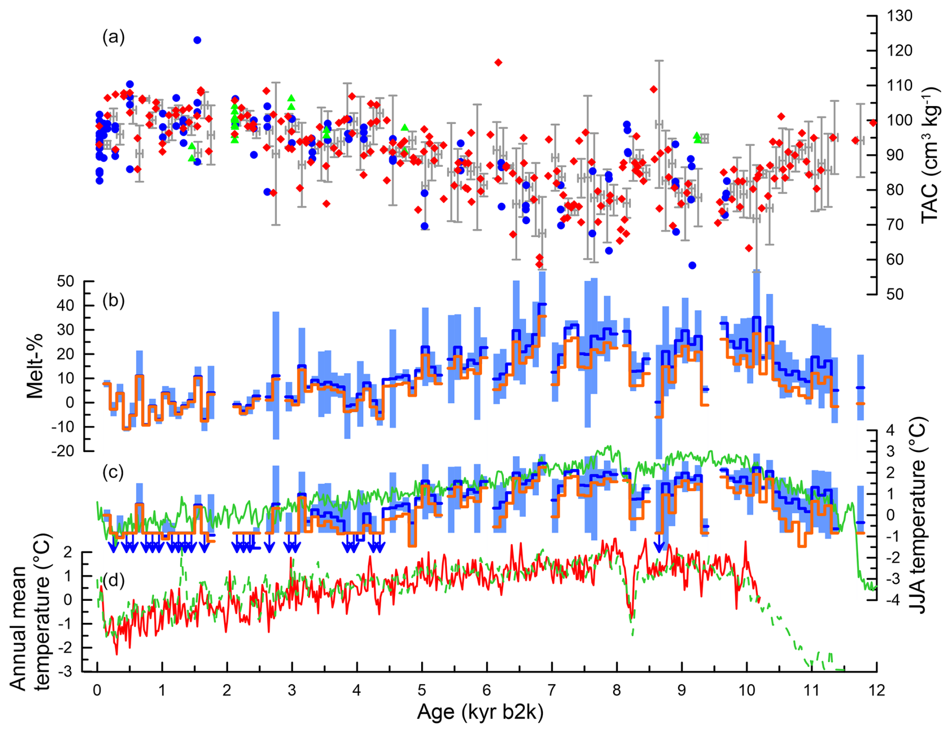
Figure 4 RECAP Holocene TAC with corresponding melt percentage and derived summer temperature all presented on the RECAP GICC05 ice timescale b2k (before 2000 CE) together with other temperature estimates. (a) TAC from PICE, PSU-CH₄, and PSU-δ¹⁵N is shown as blue dots, red diamonds, and green triangles, respectively, with 100-year averages and 1σ standard errors shown in grey. (b) Melt fractions calculated from the 100-year-averaged TAC that have been corrected for insolation effects and those that are uncorrected are shown as orange and dark blue step plots, respectively. The light blue bar chart gives the 1σ standard errors for the uncorrected melt fraction. Note that TAC larger than the modern average (see Sect. S6.2) results in negative melt percentage values. (c) Deviations from modern JJA (June, July, and August) temperatures calculated from the 100-year-averaged melt fractions. Here, 0 equals the average from 100–200 yr b2k. Melt fractions corrected for insolation effects and uncorrected melt fractions are shown as orange and dark blue step plots, respectively. The light blue bar chart gives the 1σ standard errors for the uncorrected melt fraction. A melt percentage below 2.5 % indicates temperatures colder than −5.5 °C according to the simulations. The arrow indicates that JJA temperatures are lower than or equal to −5.5 °C (corresponding to −0.84 °C relative to present day, as defined above). The solid green line shows JJA temperature calculations for Renland (Buizert et al., 2018). (d) The solid red and dotted green lines are the Renland annual mean temperature reconstructions from Vinther et al. (2009) and Buizert et al. (2018), respectively.

5.1.1 Holocene summer temperatures inferred from melt fraction

We now use the estimated melt fraction to infer local summer temperature at Renland and make use of an extension to the subsurface scheme of the HIRHAM5 regional climate model by Langen et al. (2017). The extrapolated temperatures from melt fractions suggest that Holocene summer temperatures in Renland were ∼ 2 to 3 °C warmer than present-day values (Fig. 4). This is consistent with the summer temperature reconstruction from Buizert et al. (2018). It is also consistent with the annual mean temperature reconstructions from the δ¹⁸O signals of the Agassiz and Renland ice cores that reveal that Greenland temperatures were higher than present-day values by ∼ 2 °C during the Holocene Climate Optimum (Vinther et al., 2009). GRIP paleo-temperatures interpreted from the δ¹⁸O profile and borehole temperature measurements also reveal that Greenland was warmer during the Holocene Climate Optimum (8–10 kyr b2k, boreal) by ∼ 3 to 4 °C (Johnsen et al., 1995; Dahl-Jensen et al., 1998). We note that melt layers are basically missing in the last 2 kyr, increasing only in the last century. This is in line with the observations from Taranczewski et al. (2019) based on line scan images.

5.2 Previous interglacial

Greenland surface temperatures were warmer at the end of the previous interglacial period than in the Holocene. At NEEM, it is estimated that the temperature peaked at 8±4 °C above the mean of the past millennium at 126 kyr b2k (NEEM Community Members, 2013). GISP2 δ¹⁸O records also indicate temperatures ∼ 4 to 8 °C warmer than present around 126–128 kyr b2k (Yau et al., 2016).

The TAC signal of RECAP in the previous interglacial section (> 119 kyr b2k) has incongruously low values (as low as ∼ 20 cm³ kg⁻¹, Fig. 5). It is likely that this is due to melt occurring due to increased temperatures. Applying the same metric as for the Holocene, the observed low TAC originates from temperatures at least 5 °C warmer than today. This estimate disregards insolation changes comparable between 120 kyr b2k and today. Higher temperature results in higher pore volume (Martinerie et al., 1994), which in turn results in higher TAC. For each degree Celsius of increase, the pore volume becomes half a percent larger. Therefore, we see our estimate of 5 °C warmer as a minimum. This assumes that none of the TAC changes are caused by elevation changes. If the higher temperature has led to a decrease in the Renland ice cap, TAC has to increase, again making the estimated 5 °C temperature change a minimum.

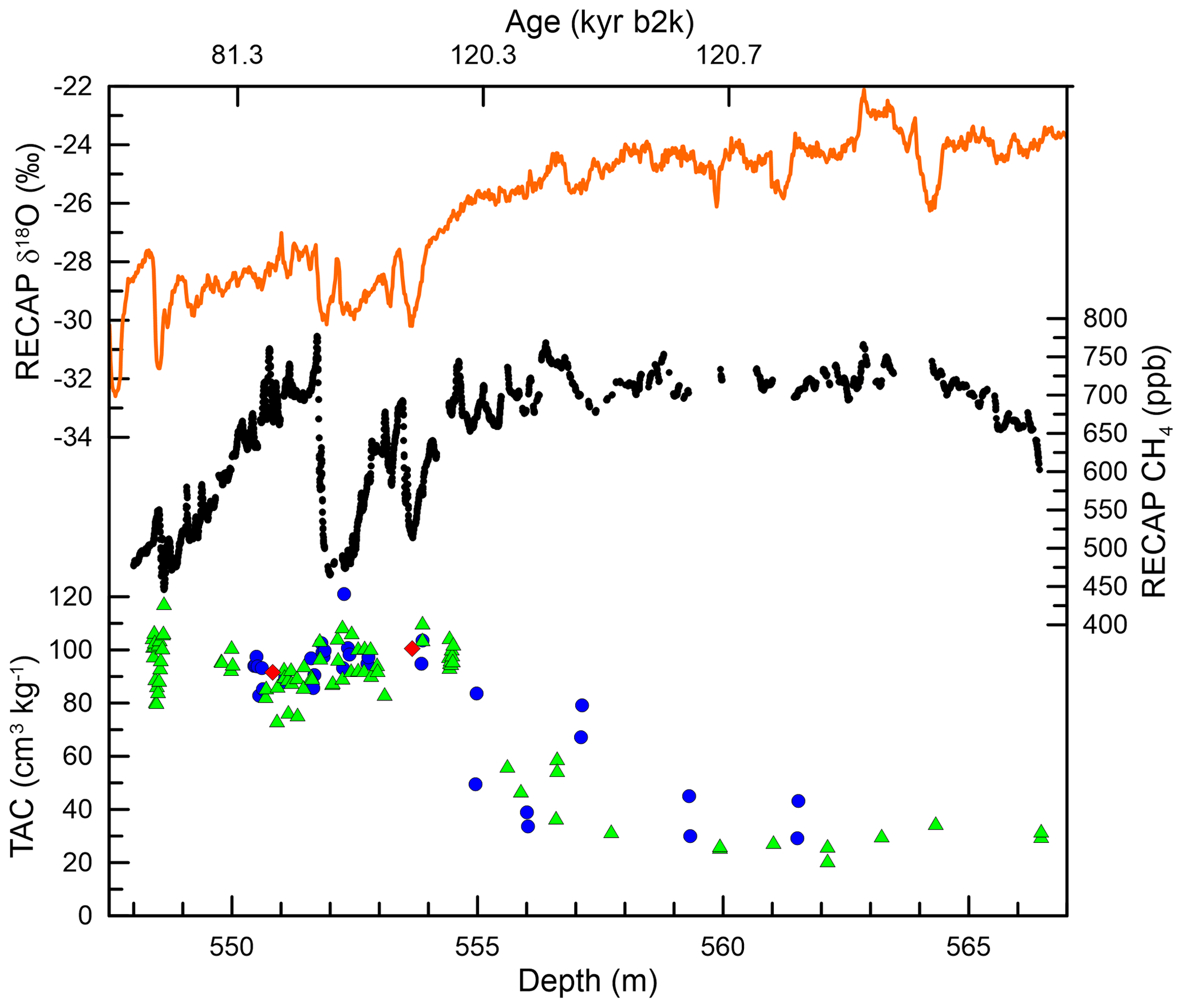
Figure 5 RECAP section showing low gas content starting around 555 m below the surface. TAC from PICE, PSU-CH₄, and PSU-δ¹⁵N is shown as blue dots, red diamonds, and green triangles, respectively. RECAP δ¹⁸O data (Gkinis et al., 2024) are shown in red, while online CH₄ data are shown as black dots. The data are presented with their depth on the lower x axis and the RECAP GICC05 ice timescale b2k (before 2000 CE) on the upper x axis.

Generally, melt layers lead to spikes in the CH₄ record due to the higher solubility of methane compared to bulk air or in situ production (see e.g. NEEM Community Members, 2013). TAC from the NEEM ice core in the previous interglacial shows low TAC values with spikes in the CH₄ and N₂O records, which is a clear indication of the presence of surface melt (NEEM Community Members, 2013). Surprisingly, we do not see spikes in the online CH₄ record of RECAP in the previous interglacial section (Fig. 5). The low gas content of the ice core in combination with the extremely low depth resolution (554–562 m corresponds to 119 to 120.8 kyr b2k) smoothed the CH₄ record. The melt spikes are potentially just not visible any longer.

5.3 RECAP TAC during D-O events

The TAC of RECAP in the glacial section (11.7 to 119 kyr b2k) shows overall similar values to those at present day (Fig. 2). However, like for NGRIP (Eicher et al., 2016), we find TAC variations associated with D-O events that are not related to elevation. Generally, in the vicinity of the D-O events the RECAP TAC signal drops rapidly, recovering after a few hundred years (Fig. S9a–d). The variations we see are on the order of 10 %–20 %. If those changes were related to elevation changes, they would correspond to changes of several hundred metres, which is unrealistic over only a couple of hundred years. It is more likely that the changes are related to changes in pore volume. Similar effects have been observed in the NGRIP core (Eicher et al., 2016). An increase in temperature with constant pore volume will result in a small reduction in TAC. This effect is slow to take effect because changes in surface temperature must first reach the close-off depth through thermal diffusion. Once steady state is reached, the effect is counterbalanced by a slightly bigger pore volume (Martinerie et al., 1994). As for the NGRIP site (Eicher et al., 2016), we dismiss synoptic pressure changes as a primary cause for the observed changes in TAC. To analyse the effect further and compare to the NGRIP site, we took the following approach.

Dynamical effects in TAC can be expected from the moment of change until a new steady state is established. At a D-O event this is when the higher accumulation snow has reached close-off. To create a general picture of what is happening in the firn column, we decided to produce a stacked plot over D-O events for RECAP and also NGRIP TAC records. The time period considered, corresponding to the time it takes for surface snow to arrive at close-off, is the Δ age. Methane and temperature changes have been found to occur in close temporal proximity during D-O events (e.g. Baumgartner et al., 2014). Changes in the methane concentration are recorded at the bottom of the firn column, while other changes related to D-O events like δ¹⁸O of H₂O or dust concentrations are recorded at the surface. Therefore, the depth interval to be considered for a dynamical firn change is between the depth when methane changes are observed and the depth where changes in parameters recorded in the ice occur. For the RECAP ice core, we find that this depth interval corresponding to Δ age is quite variable (see Fig. S9a–d). We lack an understanding of why this is the case.

To ensure that differences in Δage do not affect our analysis, we constructed our stacked plot over D-O events with a normalised time axis. For each event, the time axis is normalised so that the methane transition (in some events defined by change in δ¹⁵N) is set to 1 and the decrease in dust (coincident with the change in δ¹⁸O) is set to 0. We treat the Eicher et al. (2016) dataset for NGRIP in a similar way. The detailed results of this approach for RECAP and NGRIP can be found in Sect. S7.1 and Fig. S10. The results for TAC are shown in Fig. 6 as a low-pass cubic spline fit with a 200-year cutoff period according to Enting (1987) with 1σ uncertainties for the spline fit. The uncertainty is obtained by randomly varying the data points within their error before calculating 1000 Monte Carlo splines.

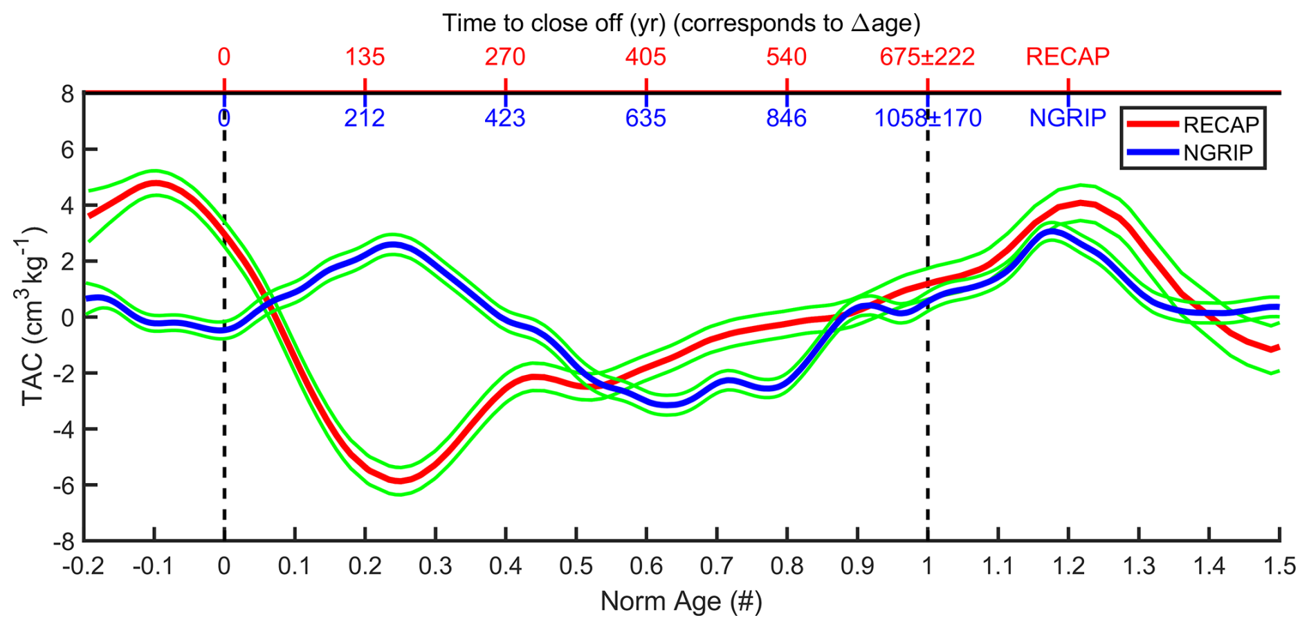
Figure 6 Effect of D-O events on TAC signals for RECAP (red) and NGRIP (blue) on a normalised age–depth scale over the past firn column. At a D-O event transition, the surface at that time is at depth 0 and the corresponding close-off is at depth 1. In other words, the zone between 0 and 1 is the past firn layer at a D-O event. The upper x axis shows the time it takes for for the rapid change to reach close-off. This corresponds to Δage. The uncertainty of ±222 and ±170 years for RECAP and NGRIP, respectively, is the standard deviation of the events considered for this stacked record (Fig. S10). The Enting (1987) spline is presented with a 200-year cutoff period, where green lines show the 1σ uncertainty in the spline.

For both cores, the TAC values on average start to decrease around the depth (time) when CH₄ starts to increase at the beginning of a D-O event. However, the minimum TAC is found before the depth (time) when the D-O event manifests as a drop in dust or increase in δ¹⁸O. For NGRIP this minimum is reached some 600 years before the snow associated with the D-O event reaches close-off, while for RECAP it is about 150 years. In addition, the drop in TAC is more significant for RECAP than for NGRIP. Overall, TAC variations associated with D-O events as recorded in RECAP are ∼ 30 % higher than in the NGRIP ice core. This may be a result of the higher accumulation and temperature at Renland.

5.4 RECAP TAC and local summer insolation

The influence of insolation on firn structure has been observed to be profound at Antarctic sites (e.g. Lipenkov et al., 2011; Bender, 2002). TAC records from Antarctic ice cores show a pronounced correlation with integrated summer insolation (ISI), as seen in EPICA DC (Raynaud et al., 2007) where the correlation is 0.86 (r²), whereas the correlation of the Greenland NGRIP glacial TAC signal is only r²= 0.3 (Eicher et al., 2016).

For the RECAP core, the correlation (r²) of the spline of ISI (sum of annual insolation ≥ 380 W m⁻²) filtered with a cutoff period (COP) of 3000 years (Enting, 1987) and the low-pass spline of glacial TAC (11.7 to 119 kyr b2k) filtered with COP of 750 years is obtained as 0.004 (Fig. S11). As outlined earlier, we may see a pattern where higher accumulation rate, due to reduced exposure time of the firn structure, results in reduced influence of insolation on TAC. However, we do not rule out that the effect may be masked in the RECAP core by the high variability associated with D-O events. A higher sample resolution allowing for the exclusion of data affected by rapid climate change from the analysis could clarify how accumulation rate and insolation interact.

5.5 Elevation change reconstructions from RECAP TAC during the last glacial maximum

Finally, we make an attempt to use glacial TAC to reconstruct ice sheet elevation. To do so we need to avoid periods of rapid climate changes. Only the last glacial maximum section fulfils that criterion and has good data coverage (Fig. 7). For a meaningful interpretation of past elevation changes, TAC data generally need to be corrected for upstream flow, summer insolation influences, surface melting, and effects of temporal variations. Since the RECAP ice core is drilled near the dome of the ice cap, upstream correction is not necessary. The melt-affected TAC data in the Holocene and the last interglacial sections are not used for elevation calculations. No melting is expected in the glacial section.

As discussed in the previous section, since the RECAP TAC has negligible correlation with ISI, insolation correction may be unnecessary. We calculate elevation with and without accounting for insolation changes, and we apply the TAC correction according to NEEM Community Members (2013). From TAC, the local ambient pressure (P_c) can be estimated, and we need to estimate local temperature (T_c) and pore volume (V_c) by applying Eq. (1). We estimate the past local temperature from NGRIP (Kindler et al., 2014), and the NGRIP record is increased by 13 °C according to the present-day difference between the NGRIP and RECAP sites. The average pressure of the 21 samples in the LGM period comes to 744±5 mbar (1 standard error). The insolation correction for this period is −10 mbar. Uncertainty in T_c and V_c is significant. Each degree Celsius changes P_c by 4 mbar, and a 1 % change in V_c results in a 7 mbar change in P_c.

The pressure P_c can now be interpreted in terms of elevation based on the barometric formula given in Eq. (2). Unknowns are the past near-surface lapse rate and the pressure at sea level.

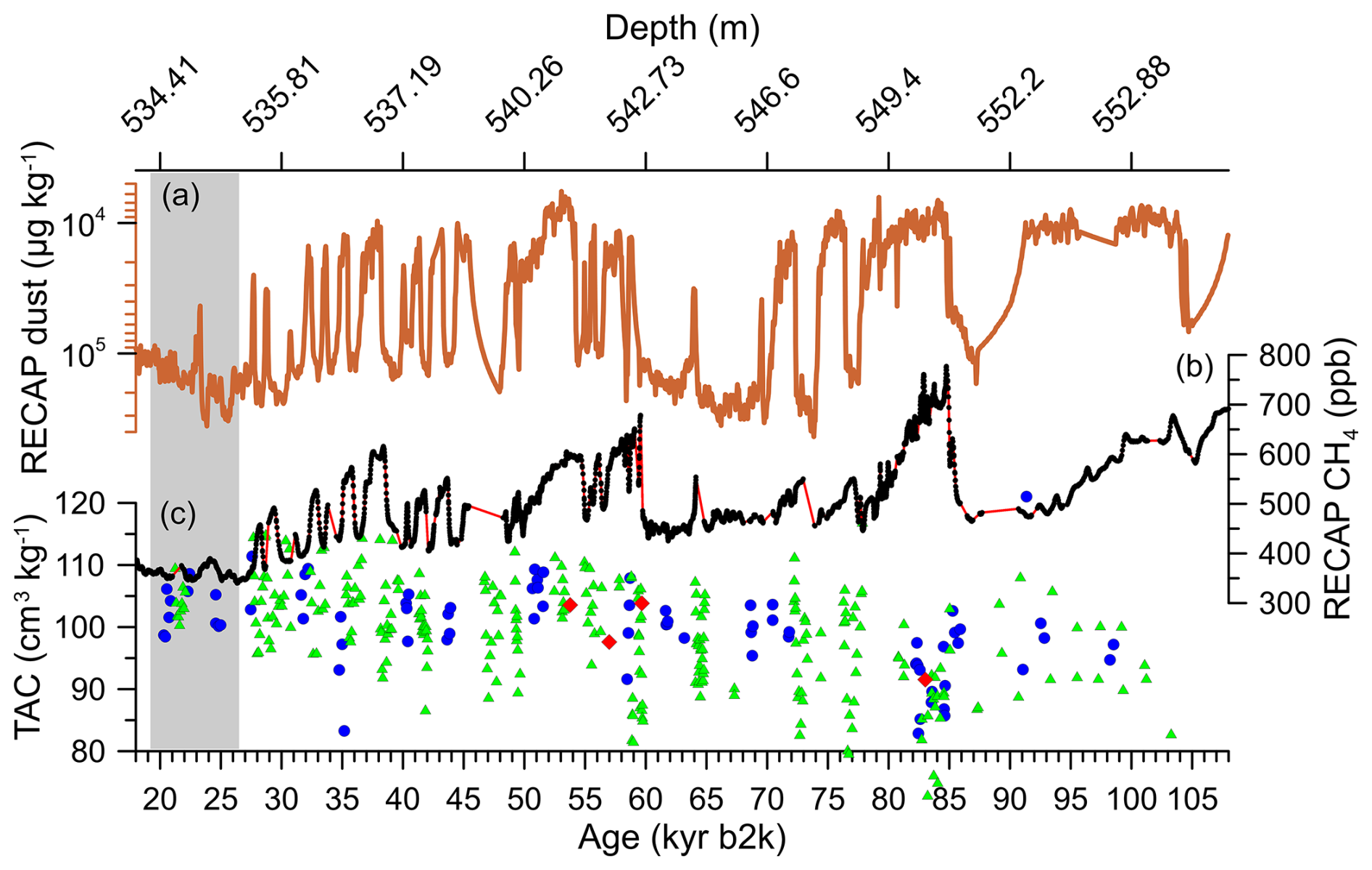
Figure 7 From top to bottom, we show the RECAP inverted dust (red) (Simonsen et al., 2019), online CH₄ (black dots and red line, note that these data are not fully calibrated and that concentrations are not absolute), and TAC (TAC from PICE, PSU-CH₄, and PSU-δ¹⁵N are shown as blue dots, red diamonds, and green triangles, respectively). Grey sections indicate the area that we use to calculate ice sheet elevation from TAC. All data are shown on the ice timescale.

Along the Greenland Ice Sheet, the annual mean near-surface lapse rate ($\mathrm{d}T/\mathrm{d}z$) has been calculated as −7.1 °C km⁻¹ based on the data obtained from the 18 automatic weather stations for the period 1995–1999 (Steffen and Box, 2001). The lapse rate varies greatly over the year from −4 °C km⁻¹ in summer to −10 °C km⁻¹ in winter (Steffen and Box, 2001). However, for present-day Renland data we calculate a near-surface lapse rate of −4.5 °C km⁻¹, and our point of reference is Ittoqqortoormiit (about 200 km from RECAP), with T_a of −7.5 °C, h_a of 0 m, and P_a of 1012.2 mbar (Cappelen et al., 2001).

Our calculations are relative to the present sea level. Krinner et al. (2000) suggest that sea level pressure at current sea level was slightly higher than today during the LGM. According to Fig. 2 in Krinner et al. (2000), this increase is between 0 and 5 mbar. In the following we disregard the uncertainty but increase the past sea level pressure to 1015 mbar. A model study on the LGM lapse rate concludes that it was about 2 °C km⁻¹ lower than today (Erokhina et al., 2017). Based on the present-day lapse rate, we calculated a LGM lapse rate of −6.5 °C km⁻¹. One could argue that the observed lapse rate for Renland of today is above the observation for Greenland since we measure the temperature in the RECAP firn. We do know that there is melting occurring today, and we therefore may underestimate the annual mean temperature at Renland. Therefore, we also calculate this using the lower lapse rate of −9.1 °C km⁻¹ (again lowered by 2 °C km⁻¹ from modern values).

Due to the topography of the ice sheet, the expectation is that the Renland ice sheet elevation is similar to today at 2340 m above present see level. Without insolation correction we calculate 2259 and 2286 m for lapse rates of −7.1 and −9.1 °C km⁻¹, respectively. Including insolation correction, the numbers climb to 2354 and 2384 m for the two cases, respectively. The statistical uncertainty is ±50 m (1 standard error), which does not include any uncertainty in V_c or T_c. For example, including a 2 °C uncertainty in T_c combined with a 2 % uncertainty in V_c increases the uncertainty in the calculations to ±220 m, which is enough that any of the four calculations covers the assumed ice sheet elevation of 2340 m above present sea level for the LGM. The RECAP site did not change significantly (within error) between the LGM and today. Hence, the results are coherent with the prime hypothesis of Vinther et al. (2009) that the Renland ice cap did not change in elevation through time.

6 Conclusion

We measured TAC back to 121 kyr b2k from the Greenland RECAP ice core. The TAC signal has unexpectedly low values in the early Holocene (6 to 9 kyr b2k) and toward the end of the last interglacial (119 to 121 kyr b2k). The low TAC values in the Holocene period point to melt events, as corroborated by elevated CH₄ values in the RECAP core (Diana Vladimirova, personal communication, 2019). Melt fractions calculated from the RECAP TAC signal in the Holocene are in turn used to interpolate the summer surface temperatures (subsurface HIRHAM5 model). Summer temperatures in the early Holocene at Renland were ∼ 2 to 3 °C warmer compared to today. This finding is in agreement with similar findings from Greenland ice cores and model calculations. During the previous interglacial we see significant melting that let us conclude that temperatures at Renland were at least 5 °C warmer than today.

The influence of local summer insolation ≥ 380 W m⁻² on the TAC signal of Renland is minimal, as indicated by the correlation coefficient (r²) of 0.004. Elevation of the Renland ice cap is calculated from the last glacial maximum TAC data. These elevation calculations encompass the uncertainties that arise from the assumption of the lapse rate, temperature, and pressure gradients that existed in the past and sum up to ±220 m. The elevation was similar to today (within this large uncertainty). During D-O events, RECAP TAC shows significant variations that are larger than in other ice cores. How these variations come about is currently not understood. The stacked data analysis that we performed for RECAP and NGRIP shows that changes in the firn structure must occur within the firn column during events of rapid climate change.

Reconstructing the elevation history of ice sheets is crucial for predicting how they will respond to warming. However, recent findings cast doubt on the reliability of elevation reconstructions based on TAC, especially in Greenland over shorter millennial timescales. We need to explore the physical reasons behind short-term TAC changes and quantify insolation effects before we can confidently interpret TAC data for elevation shifts.

Appendix A

We use the estimated melt fraction to infer local summer temperature at Renland. Langen et al. (2017) extended the subsurface scheme of the HIRHAM5 regional climate model to include snow densification, varying hydraulic conductivity, irreducible water saturation, and other effects on snow liquid water percolation and retention to calculate meltwater production. Langen et al. (2017) evaluated melt amounts and melt extents against in situ and satellite-based observations. The model allows us to derive an empirical relationship between melt fraction and temperature in the region. The model takes weather forcing at the surface from the regional climate model HIRHAM5 over the period 1980–2016 (forced in turn by ERA-Interim on the lateral boundaries) and calculates surface melting (of snow and bare ice), vertical percolation, retention, refreezing, densification, grain growth, runoff, and surface mass balance. The subsurface calculations are performed on the 5.5×5.5 km grid of HIRHAM5. Over 15 grid cells centred on the RECAP drill site (Fig. A1), we gather total annual meltwater production and JJA average temperatures from each of the years 1980–2016 (giving $\mathrm{15}\times \mathrm{37}=\mathrm{555}$ data points).

Meltwater production is converted into melt percentages using an observed approximate annual accumulation rate of 50 cm ice equivalent. The data points are then divided into 0.5 K bins with respect to JJA temperatures. A mean melt percentage is calculated for each bin (Fig. A1). An exponential fit describes the resulting relation between JJA temperatures and melt percentages as melt percentage is equal to b ⋅ exp($a\dot{T}$), a is 0.6732, and b is 179.02, where T is the mean JJA surface temperature in degrees Celsius.

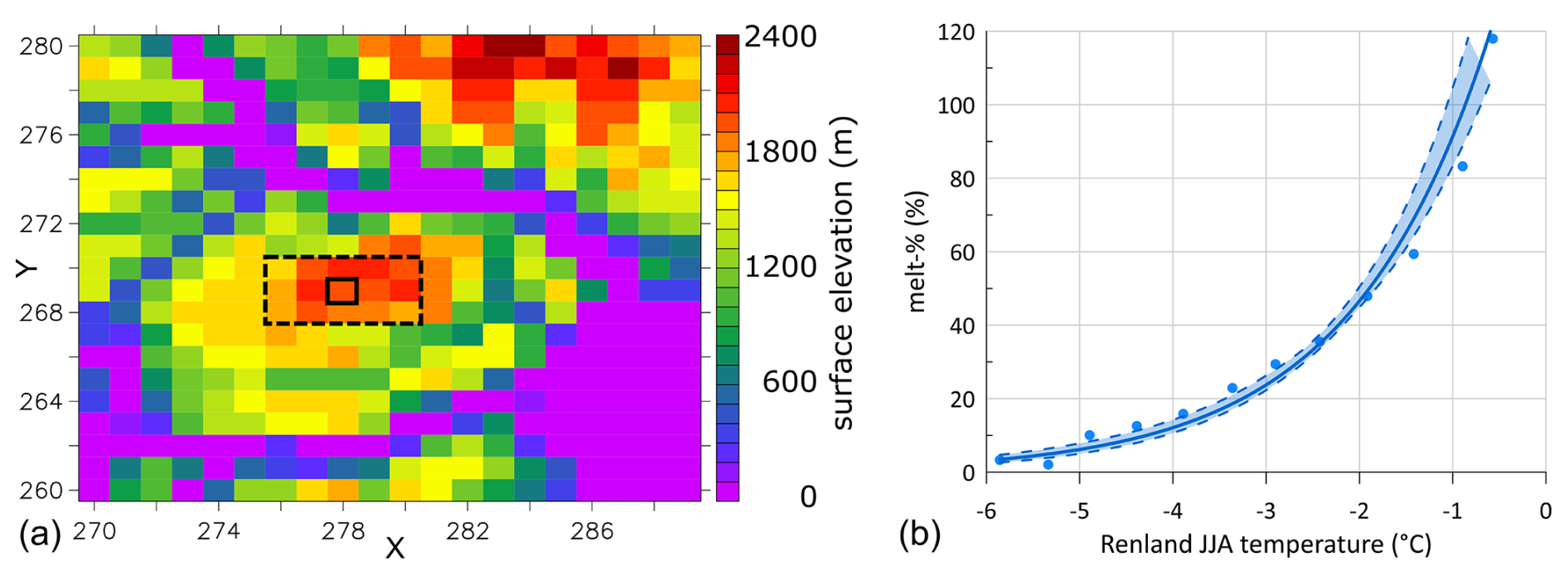
Figure A1 Panel (a) shows 15 grid cells (inside the dashed square) centred on the RECAP drill site (the solid square) as part of the subsurface calculations performed on the 5.5×5.5 km grid of HIRHAM5. Panel (b) shows the Renland surface melt percentage vs. JJA temperatures.