CYCLIM: a semi-automated cycle counting tool for generating age models and palaeoclimate reconstructions

Counting annual-scale fluctuations, such as geochemical cyclicity or visible growth bands, within a climate archive can yield extremely high-precision chronological models. However, this process is often time-consuming and subjective, and although various software packages can automate this process, many researchers still prefer to count manually given its technical simplicity and transparency. Here we present a new tool that combines the time saved by automation with the flexibility afforded by expert judgement. CYCLIM uses a matched filtering approach to detect cyclicity and then allows the user to inspect and refine the automated output whilst also quantifying age uncertainty. The presented framework speeds up cycle counting by automating the first-pass of the count while also retaining the benefits of a manual count by allowing for post-analysis tuning. Across three examples using published palaeoclimate reconstructions, the automatic output found 96.0 % of the cycles, with a false positive and false negative rate of 3.4 % and 4.0 %, respectively. This means that only ∼ 7 cycles per 100 need to be corrected manually, making cycle counting with CYCLIM an order of magnitude faster than by visual inspection.

1 Introduction

Palaeoclimate reconstructions are the principal method to put modern climate trends within a longer-term variability. These techniques use proxies recorded in natural archives to track past changes in the climate system, and so one of the key steps in developing palaeoclimate reconstructions is translating depth (or growth) to the time domain. Chronologies are derived using a variety of techniques such as radiocarbon or uranium-series dating, but usually they can only supply a limited number of points because of sample material, analytical costs, and time constraints (Breitenbach et al., 2012). Cycle or layer counting, although relative, offers a powerful alternative, often reaching sub-annual precision (Comboul et al., 2014; Forman et al., 2025; Ridley et al., 2015).

Rhythmic layering and/or cyclicity in palaeoclimate archives can reflect seasonal to annual environmental variability, which can serve as the basis for a chronology. Cycle counting involves identifying and quantifying these repeating visual (e.g., colour or texture) or geochemical (e.g., stable isotopes or trace elements) parameters. However, prior to performing a count, the annual-scale fluctuations need confirmation as truly annual both with independent chronological validation and a theoretical basis for the processes involved in generating the periodicity. Many natural archives are amenable to cycle counting methods, including: (1) tree rings by preserving annual growth rings (e.g., Anchukaitis and Evans, 2010); (2) corals through density bands and geochemical signatures (e.g., Goodkin et al., 2005); (3) ice cores via multiple records such as dust, conductivity, and stable isotopes (e.g., Winstrup et al., 2019); (4) lake/marine sediment through visible varves (e.g., Wick et al., 2003); and (5) speleothems via physical laminae and geochemical cyclicity (e.g., Tan et al., 2006). Whereas cycle counting is prone to error via missing/ambiguous cycles in addition to lacking the absolute dating precision afforded by some radiometric methods, it offers unparalleled temporal resolution in many contexts and can augment existing chronologies, particularly when anchored to a known age.

The process of cycle counting is often time consuming and subjective, so many studies have presented analytical tools to automate the process. Some archives have purpose-built chronological packages due to the nuances of the systems. Tree ring chronologies typically combine records from multiple trees using techniques such as cross-dating to overcome inaccuracies arising from rings in one record that are missing or false (St. George, 2014). Similarly, ice core chronologies may require correcting for thinning and compaction using techniques such as thinning functions and ice flow models (Kahle et al., 2021). For this reason, archive-specific tools such as dplR (Bunn, 2008) and the hidden Markov models (HMMs) algorithm presented by Winstrup et al. (2012) exist for dating tree rings and ice cores, respectively, although, if the dataset permits, general tools could still yield accurate age models for these records. These general tools are either applied to images/scans of the archive to count visible layer boundaries or to depth profiles extracted from the archive to count detectable cyclicity. A degree of overlap exists between these two methods because images/scans can convert into intensity profiles such as greyscale or fluorescence to then undergo cycle detection using similar signal processing techniques to those of non-image-based tools. Visual packages exist for counting both varved sediments (e.g., Weber et al., 2010) and speleothems (e.g., Sliwinski et al., 2023) using techniques like machine learning. Signal processing algorithms simply use a depth-proxy record and identify cycles via statistical techniques like peak detection, making them very versatile. Smith et al. (2009) developed a trace element cycle counting algorithm that uses an estimate of mean cycle width obtained by spectral and wavelet analysis. The algorithm also uses two threshold criteria: (1) a minimum cycle amplitude, fixed to a local standard deviation of signal variance; and (2) a minimum inter-cycle separation, calculated relative to the preceding detections. Nagra et al. (2017) devised a multi-proxy approach for counting annual trace element cycles in speleothems. Each trace element transect is normalised and concatenated before undergoing a principal component analysis (PCA), after which principal component 1 (PC1) is passed to a peak counting algorithm. This algorithm uses a prior estimate of annual growth rate as a sampling window and sets thresholds relative to the mean cycle for determining whether a detection is false or missing. However, many researchers still opt to count by inspection, partly because it offers greater flexibility and because the variability among proxy records can impede the effectiveness of automated techniques.

Combining the advantages of both automation and expert judgement, here we present a Python-based application (CYCLIM) that automatically detects cyclicity before allowing user-guided refinement of the results. Cycles are detected using matched filtering with a Gaussian kernel and sections of ambiguous cyclicity are identified. Within the interface the user can then review the output and adjust boundaries by removing spurious detections and/or adding in new cycles. Additionally, the user can quantify algorithmic uncertainty using a noise perturbation-based Monte Carlo approach. This methodology provides a flexible and reproducible framework that streamlines the process by automating the initial detection phase while preserving the control necessary for dealing with the heterogeneity and noise of proxy records. By facilitating both efficiency and supervision, CYCLIM enhances the speed, accuracy, and transparency of cycle counting.

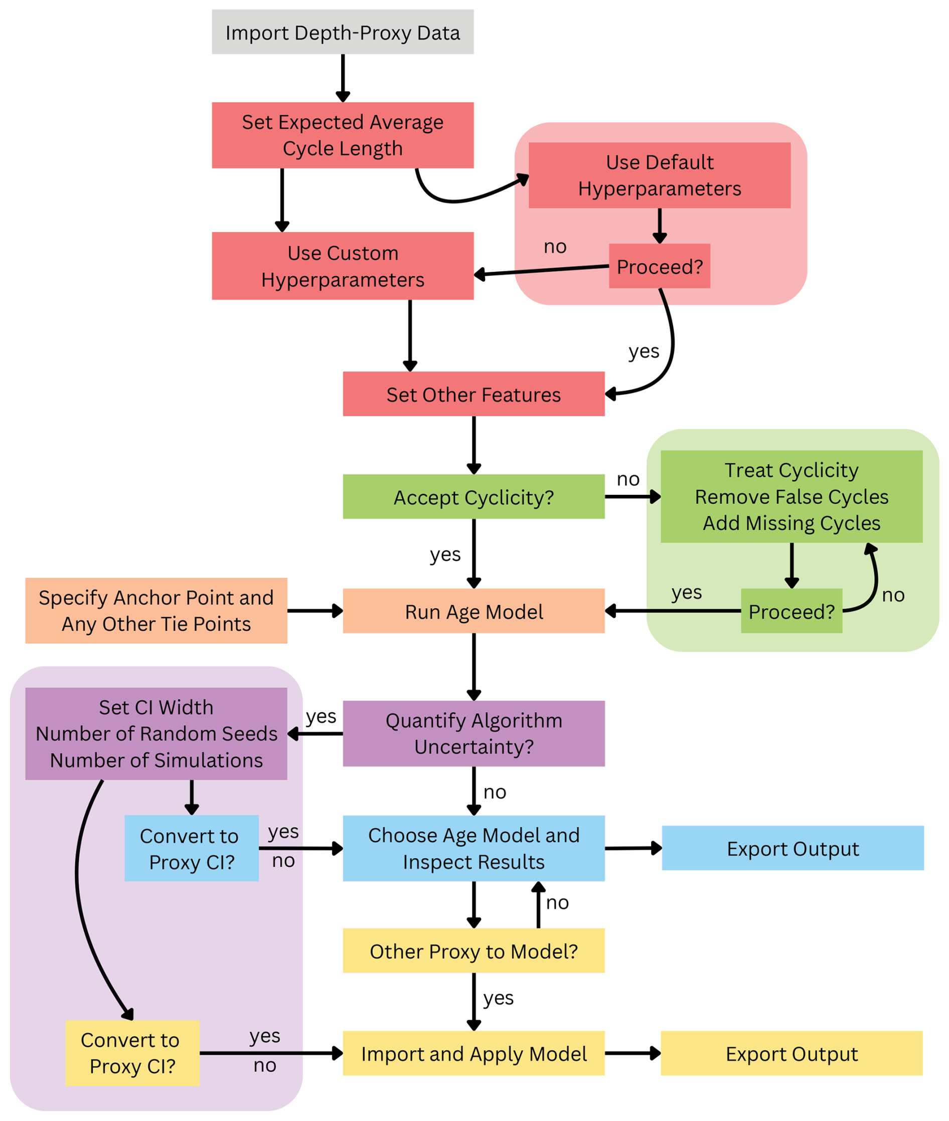
Figure 1 A schematic overview of the CYCLIM workflow. Colours denote the step of the GUI in which each element occurs. Step 1 (grey): upload and confirm the depth-proxy data. Step 2 (red): hyperparameter set-up and minima detection. Step 3 (green): manual inspection of the output minima with the ability to add or remove entries. Step 4 (orange): specify chronological constraints and run age model. Step 5 (purple): quantify algorithmic uncertainties. Step 6 (blue): choose manual/automatic age model, convert uncertainties and view final output. Step 7 (yellow): import and model additional depth-proxy datasets using the age model chosen in Step 6.

2 Interface and Methods

2.1 Graphical User Interface (GUI) Overview

The CYCLIM algorithm (Fig. 1) uses a semi-automated approach whereby the user can optimise the algorithm by tuning its hyperparameters and enabling additional features, before allowing inspection and refinement of its output. First, the interface prompts the user to import the depth-proxy dataset for counting. The depth-proxy dataset should: (1) have sufficient signal-to-noise to distinguish annual cyclicity from background noise; (2) exhibit no substantial or consistent change in cycle length; (3) have approximately equally spaced datapoints; and (4) ideally contain no missing values. The algorithm can tolerate a few missing values provided they are removed prior to counting and maintain a near-perfect consistency in sampling rate. CYCLIM uses matched filtering to extract the annual signal, which can either be done automatically, or the user can manually refine the algorithm (see Sect. 2.2). Minima are then identified in the matched filter output and are used as cycle boundaries. Additionally, there is the option to apply gap treatment, which addresses intervals with no detection by inserting estimated cycles, and cycle tuning, which refines the boundary positions to local minima in the original record (see Sect. 2.2). Post-detection the user can inspect the cycles boundaries that the algorithm detects to remove erroneous detections and add in any missed by the algorithm. The system tracks the origin of each minimum (i.e., whether it was added at the matched filtering stage, gap adjustment or manually by the user) and shown in the GUI. This ensures that artificial cycles resulting from the gap adjustment stage are distinguishable from filter- or user-defined minima, allowing for different assessment.

After confirming the count, the user specifies an anchor point to temporally constrain the annual boundaries, which could be the collection year, the radiocarbon bomb spike depth, or a U-Th point. There is also the option to upload a full list of chronological tie points for comparison and specify the sub-annual timing of the minima. CYCLIM then uses piecewise cubic Hermite interpolating polynomial (PCHIP) interpolation to assign an age value to every datapoint in the depth-proxy dataset by estimating ages between the detected cycle boundaries. At this point there is the option to quantify algorithmic uncertainty and devise a confidence interval for the age model (see Sect. 2.3). Furthermore, users can choose to enable the translation of the proxy values onto a time-certain axis, thereby converting age uncertainty into proxy uncertainty. Post-analysis, the user can export the minima locations with their origin (supporting further age modelling incorporating other chronological methods) and the age-converted dataset. Finally, the system facilitates the import and depth-age conversion of any additional proxies from the archive using the age model derived prior, provided it is within the same depth range. Once converted, the user can extract the age-converted data for further analysis.

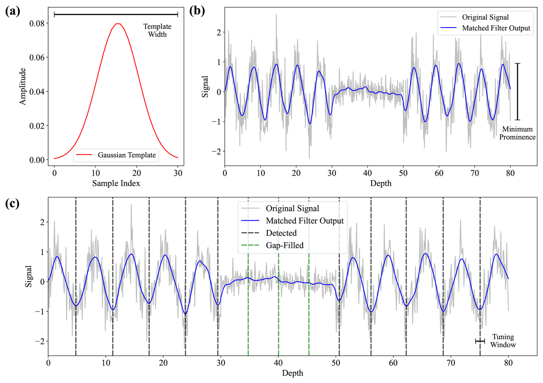
Figure 2 A schematic overview of the matched filtering technique. (a) The Gaussian template used for matched filtering, which is set to the number of datapoints corresponding to half the estimated average cycle length of the hypothetical dataset. (b) The hypothetical dataset (grey) and the convolved matched filtering output (blue). (c) The record in (b) with the detected cycle boundaries (vertical black dashed lines) and the inserted boundaries during gap treatment (vertical green dashed lines).

2.2 Cycle Detection

Cycles are extracted using a matched filtering approach designed to enhance the defined annual-scale cyclicity within the depth-proxy dataset (Fig. 2). A Gaussian-shaped template is constructed to approximate the expected waveform of the cycles. The user can manually specify the template width (w) or the CYCLIM algorithm will automatically set the template width to correspond to half the number of datapoints that comprise the average cycle length, which is specified by the user. The method uses a half-cycle length because matched filtering with a Gaussian template produces strong responses for segments that resemble either the template's standard orientation (peaks) or its inverse (troughs). This approach allows the filter to detect cycles without requiring knowledge of the full waveform shape, emphasising general pattern similarity and thereby making it robust to asymmetry or obscuration due to noise. Because the template centres around a single point, the window must be odd. If the calculation yields an even number, the algorithm expands the window by one. The Gaussian template is defined as a normalised function:

$$\begin{array}{}\text{(1)}& G\left(\mathit{t}\right)={\displaystyle \frac{\mathrm{1}}{Z}}\cdot \exp \left(-{\displaystyle \frac{t^{\mathrm{2}}}{\mathrm{2}{\mathit{\sigma }}^{\mathrm{2}}}}\right),\end{array}$$

where t is an index vector centred on zero, $\mathit{\sigma }=\frac{w}{\mathrm{6}}$, and Z is a normalisation constant, computed as the sum of the unnormalised Gaussian values, that ensures the template has unit area. The choice of σ ensures that > 99 % of the Gaussian's area falls within the selected window.

The proxy signal data is then convolved with G(t) to yield a matched filter output:

$$\begin{array}{}\text{(2)}& Y\left(\mathit{t}\right)=(y\ast G)\left(\mathit{t}\right),\end{array}$$

where ∗ signifies convolution. The resulting signal Y emphasises the regions of the original y signal that resemble the template shape, thereby enhancing the cyclic component while reducing high-frequency noise.

Because the algorithm counts cycles using minima, it inverts the filtered signal before performing peak detection. Peaks in the inverted signal correspond to points that exceed their immediate neighbours and surpass a minimum prominence criterion. This threshold suppresses false detections caused by remaining signal noise and allows the user to manually set the value or automatically assigns it a value equivalent to 2.5 % of the range in y between the 2.5th and 97.5th percentiles.

Following the initial detection stage, the algorithm can tune the found minima to a local minimum in the original dataset. If enabled, this feature uses the tuning window to search the nearby points in the raw signal of each minimum detected by the matched filter for a true minimum. In custom mode the user specifies the width of this tuning window, but in default mode the algorithm sets the window to a quarter of the full cycle length, approximating a 3 month period, whilst ensuring the window is odd by expansion where necessary. This ensures that final positions remain within the same season and correspond to inflection points in the original data.

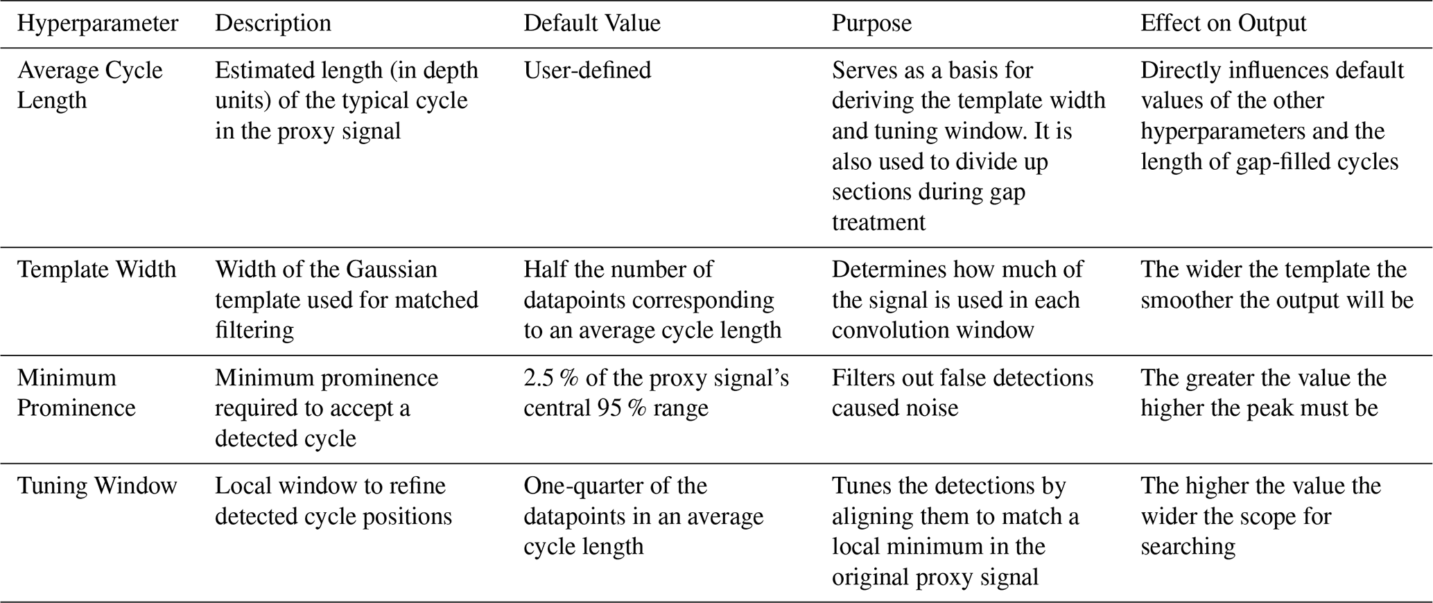
Table 1 The hyperparameters used in the CYCLIM algorithm and their role.

To maintain accuracy and avoid undercounting, the algorithm includes an additional step to treat missing sections of the record and/or intervals where cyclicity is indistinguishable from background noise. If enabled, and no minimum appears within an interval exceeding the gap threshold set by the user, the algorithm subdivides the section at regular intervals equal to the average cycle length and tunes each to localised minima. Although this step introduces artificial cycles, it ensures that the overall count does not deviate from the underlying age model due to missed cyclicity.

The detection methodology thus uses four hyperparameters: (1) the average cycle length; (2) the template width; (3) the minimum prominence; and (4) the tuning window (Table 1). In custom mode, the user must specify values for all of the hyperparameters, whereas in default mode, only an estimate for the average cycle length is required. However, because this estimate is used to determine the value of the other hyperparameters it needs to be a fair approximation. Provided the estimate is robust, the sensitivity of the output to its exact value depends on the record's resolution and noise level. The sensitivity of the output to the choice of template width and minimum prominence is computed within the algorithm. The GUI then plots the similarity of the detected cycle boundaries relative to the current configuration as the template width and minimum prominence are varied. The template width is modified by ± 30 % and the minimum prominence value is converted to a percentage to the range in y and adjusted by ± 5 %.

2.3 Algorithmic Uncertainty Quantification

To quantify algorithmic uncertainty as an approximation of cycle counting age uncertainty, CYCLIM adopts a noise-based Monte Carlo approach. By perturbing the signal in a similar way to natural processes, we can model the algorithm's sensitivity and yield estimates of variance between counts that reflect that arising from counting error.

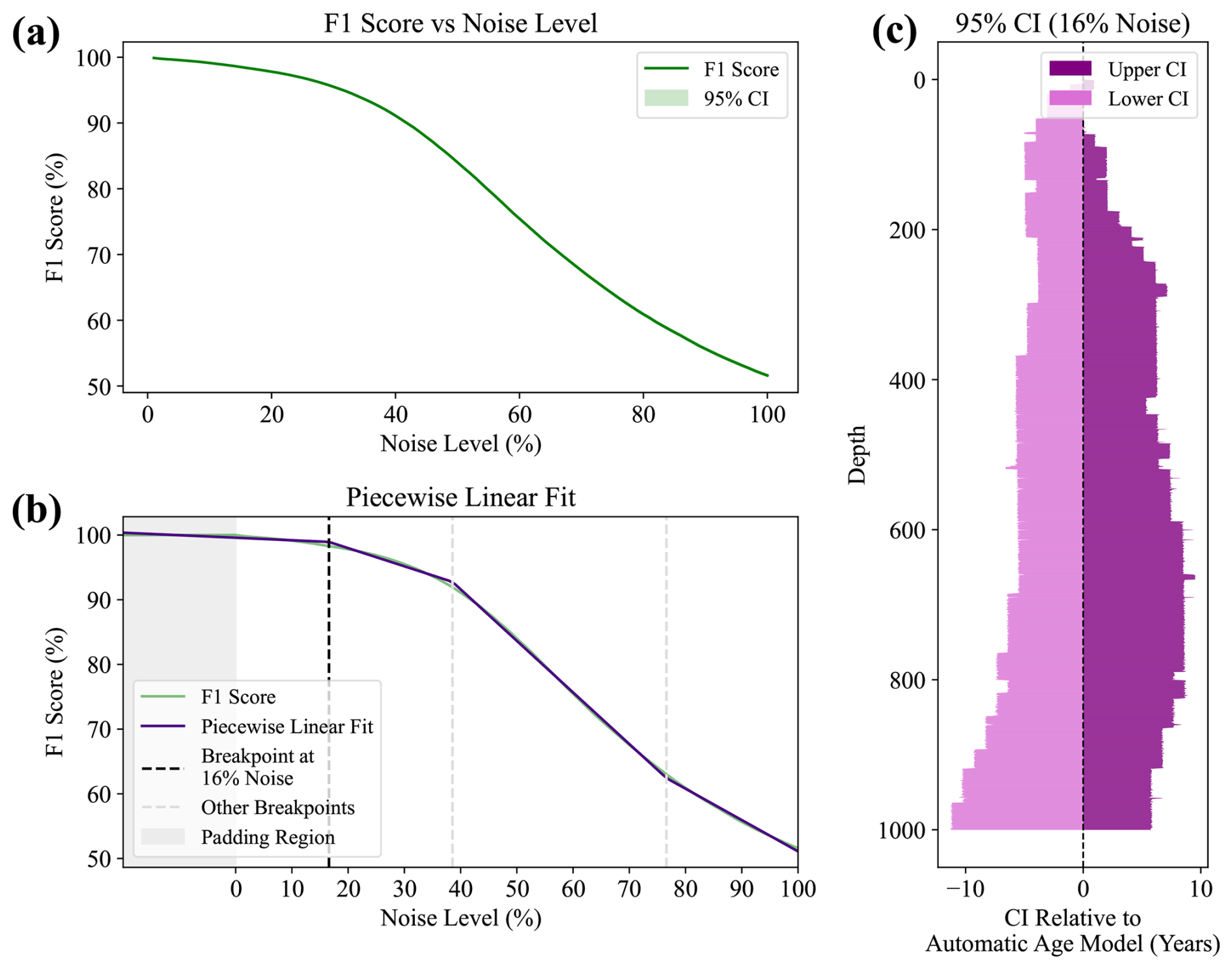
Figure 3 A schematic overview of algorithmic uncertainty calculation using a dataset of 1000 noisy sine waves. (a) The algorithm's ability to reproduce the same list of minima under increasing noise levels. (b) The breakpoint locations determined from a piecewise linear fit of four segments on the F1 score curve shown in (a). (c) The variance in number of minima detected with depth under the breakpoint level of noise. The 95 % confidence interval for 100 random seeds is shown relative to the automatic age model. Note that the asymmetry is the product of signal noise and highlights the direction of uncertainty.

First, CYCLIM stores the minima positions from the cycle detection stage, including those added by gap treatment, as a reference set. Then, for a user-defined number of random seeds, arrays of Gaussian white noise are generated of equal length and standard deviation to the proxy signal. These random signals are then progressively linearly mixed into the proxy signal from 1 % to 100 % (in 1 % increments) to simulate random error. The same algorithm used to derive the reference set is then applied to each noise level and random seed combination, and the resulting lists of detected minima are stored. Each run's performance is evaluated against the reference set using the F1 score, a harmonic mean of precision (here the fraction of output detections that are found in the unperturbed signal) and recall (the fraction of reference minima detected) based on a detection tolerance of a quarter cycle length. The analysis employs the F1 because it includes both over- and undercounting as systematic error, making it a robust metric of signal recovery fidelity under increasing noise. The mean 95 % confidence interval for the F1 scores across all seeds at each noise level is computed, producing a performance curve (Fig. 3a).

A noise level that approximates counting errors is then identified. To ensure method robustness across a wide range of input signals, this threshold is set dynamically to when algorithmic performance first begins to degrade disproportionately to the increase in noise. This noise level marks the boundary between algorithm robustness and failure, where detection accuracy becomes increasingly sensitive to small changes in noise level showing the algorithm's operational limit. Modelling the algorithmic response to lower (higher) levels of noise could underestimate (overestimate) uncertainty and so simulating at the tipping noise level avoids misrepresenting uncertainty. By using this level, the internal biases of the matched filter arising from hyperparameter choice become the salient driver of variability across random seeds. It thus exposes how stable the algorithm's output is to noise, replicating signal ambiguity due to discrete sampling. Therefore, it mimics the plausible levels of epistemic uncertainty of manual counting by perturbing the signal enough to induce detection error but without causing irreparable signal damage.

The noise level is determined using a piecewise linear fit with three breakpoints (Fig. 3b). Signal degradation with respect to noise follows an S-curve, thus having two breakpoints, but using the first would overestimate signal stability, especially in records with higher internal noise. Under these conditions the reproducibility of the reference boundaries deteriorates more linearly, suppressing and/or delaying the first S-curve breakpoint. Thus, the F1 score curve is padded, introducing a third breakpoint which finds where reconstruction fidelity first falls beyond that tolerated by the padding. This new first breakpoint derives the noise level for Monte Carlo simulation. However, because template width tends to be flexible given its use for smoothing, the threshold noise level depends on the sensitivity of the minimum prominence criterion. Therefore, if the algorithm is too sensitive to this hyperparameter choice the first breakpoint will be detected at noise levels of < 2 %. In such cases this method cannot determine the right noise level to use, and uncertainty is not quantifiable.

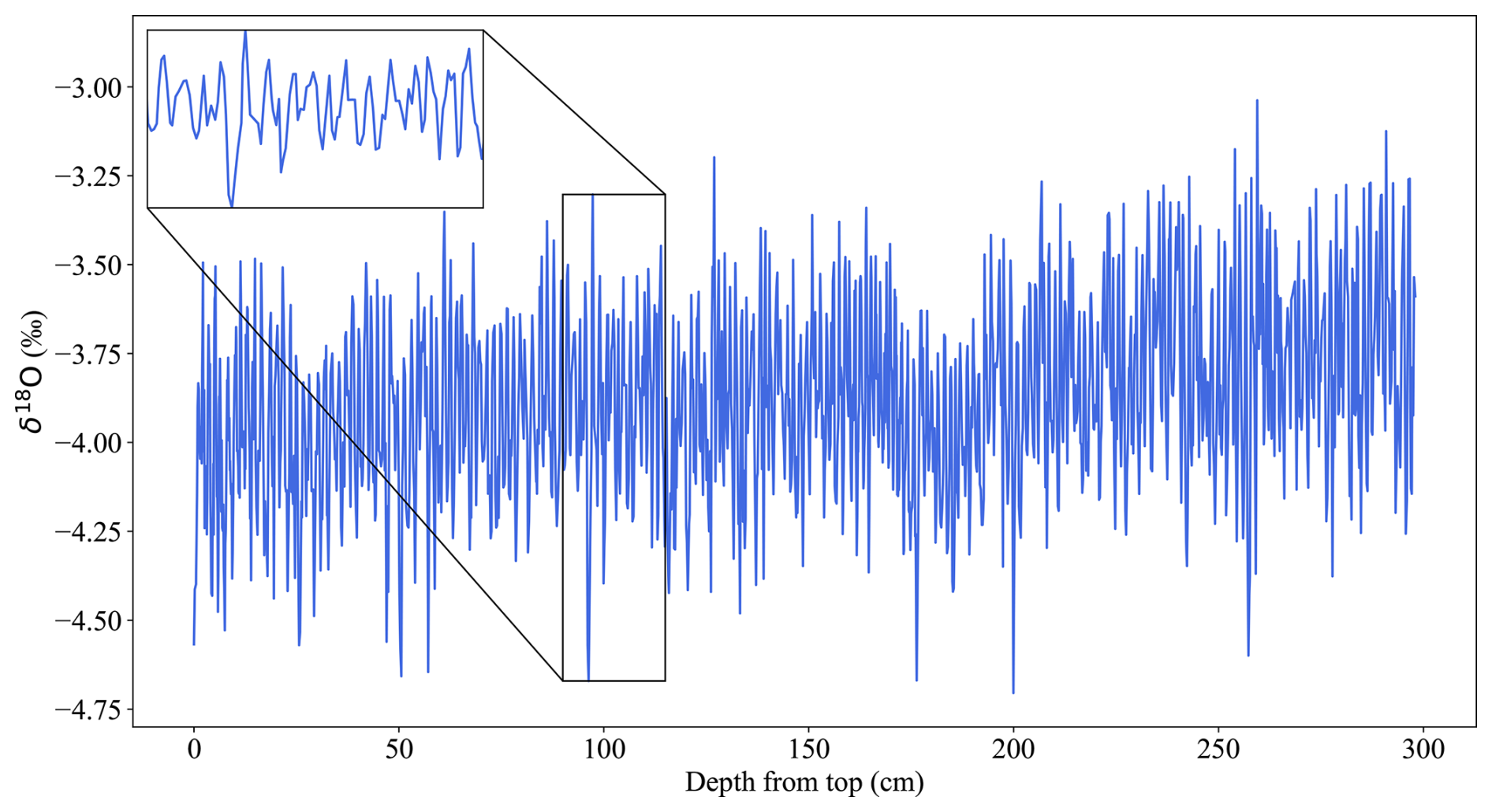
Figure 4 The depth-proxy Houtman Abrolhos Coral δ¹⁸O record (blue; Kuhnert et al., 1999). The inset shows an example interval of annual scale cyclicity.

Each of the random seeds from before are then combined with the proxy signal at the determined threshold noise level and run through the cycle detection algorithm from before. The location of each run's boundaries is stored and are converted to age models using the chronological constraints applied to the reference age model, providing a record of internal model variance. Also, if additional chronological tie points are uploaded there is the option to use them to constrain the realisations by skipping age models that plot outside of their uncertainties. The ensemble of age models is then interpolated onto the proxy's depth axis and percentile-based confidence intervals are calculated and compared to the reference age model (Fig. 3c). These uncertainties are thus not always symmetrical and can highlight whether it is more likely that cyclicity is being missed or wrongly detected by its directionality. Additionally, because this is a method to quantify algorithmic uncertainty, it is shown in relation to the automatic age model and does not apply to the manually tuned chronology. These uncertainties can be used to guide manual tuning; adding or removing boundaries beyond algorithmic uncertainties should be performed with caution, and likely only when correcting systematic bias in the detection algorithm. Finally, the age model uncertainties can optionally be translated into time-certain proxy uncertainties via ensemble-based mapping of proxy values onto the time domain.

3 Example Use of CYCLIM

To test CYCLIM's performance, we show its application to three previously published palaeoclimate records. All three show annual scale cyclicity but with varying degrees of clarity and consistency. For each example the automatically generated template size hyperparameters were used, but the minimum prominence criterion was sometimes changed due to record extrema effecting the automatic estimate. Additionally, these tests were run without knowledge of the published cycle count. The mean cycle length was extracted from the depth-proxy information and the manual tuning was performed independently, without comparison to the original paper's age model.

3.1 Records

3.1.1 Houtman Abrolhos Coral

As a first-pass test of CYCLIM's ability to detect cycles we use the coral δ¹⁸O record from the Houtman Abrolhos Islands off west Australia presented in Kuhnert et al. (1999), which exhibits very prominent annual cyclicity with a very consistent annual growth rate and low noise level (Fig. 4). The core was sampled from a living colony of Porites lutea in May 1994 and is 300 cm in length. The δ¹⁸O record likely captures past temperatures, with high-frequency fluctuations reflecting annual cyclicity. Ages were thus determined by counting this cyclicity relative to the date of collection and maxima assigned to mid-September, aligning with the coolest month. The original chronology spans 200 years (1794–1994 CE). Although the annual variability is clear throughout almost all the record, the authors note that the clarity of the δ¹⁸O cycles weakens near 1853 and 1869. Estimated age errors are 1 year per century (Kuhnert et al., 1999).

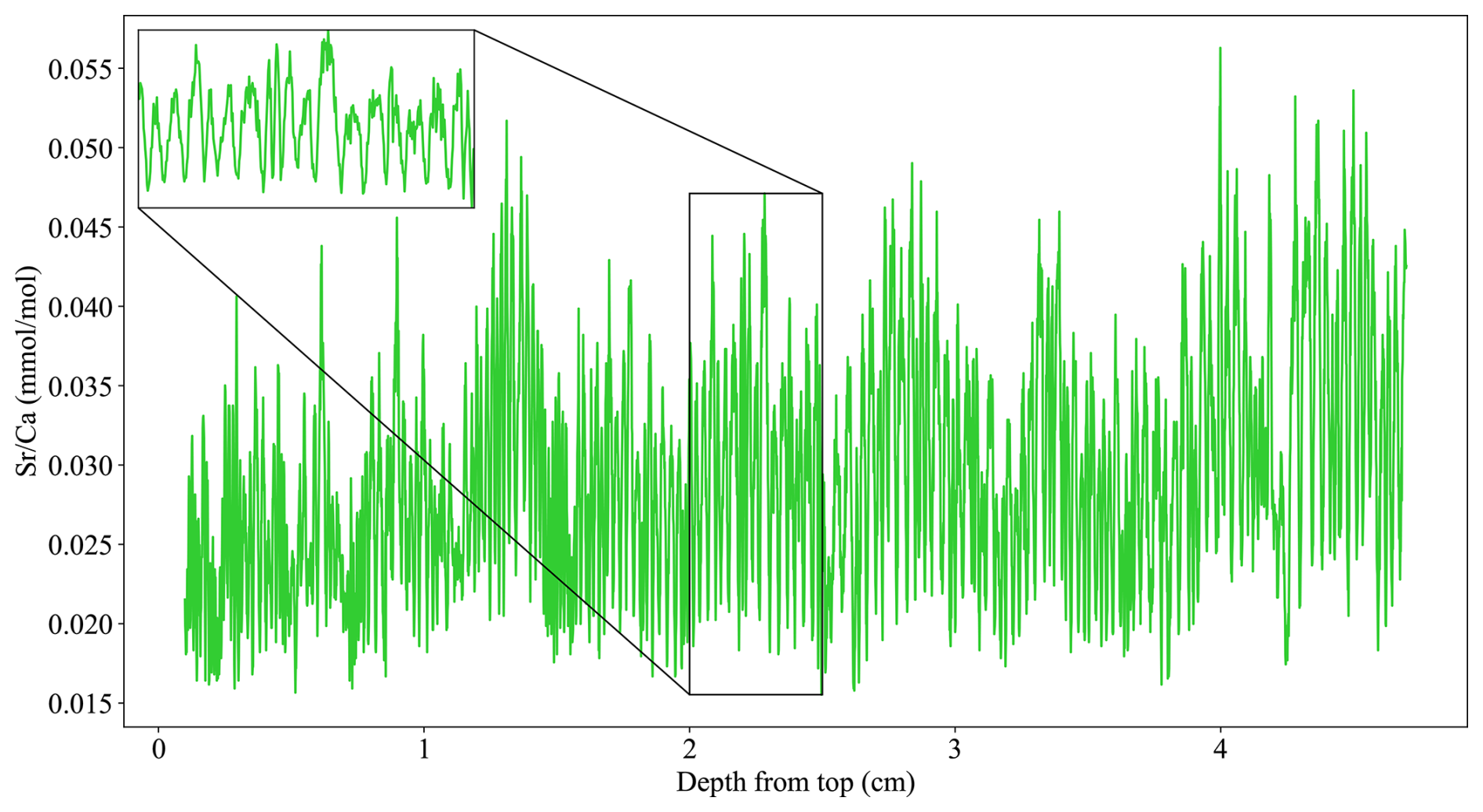
Figure 5 The depth-proxy C09-2 stalagmite $\mathrm{Sr}/\mathrm{Ca}$ record (green; Warken et al., 2018). The inset shows an example interval of annual scale cyclicity.

3.1.2 Stalagmite C09-2

Next, we use the stalagmite record presented in Warken et al. (2018) which exhibits a variable growth rate and more pronounced noise, to test the algorithm's ability to cope with inconsistent waveform characteristics (Fig. 5). The stalagmite was collected from a cave in southwest Romania in 2009 and is 70 cm tall. Trace element variability exhibits pronounced cyclicity, likely driven by strong seasonal differences in calcite precipitation rates (Warken et al., 2018). $\mathrm{Mg}/\mathrm{Ca}$, $\mathrm{Ba}/\mathrm{Ca}$, and $\mathrm{Sr}/\mathrm{Ca}$ all show annual cyclicity, but only $\mathrm{Sr}/\mathrm{Ca}$ is used here for cycle counting. Because of their relation to rainfall, minima were allocated to mid-summer. The uppermost 1 mm was lost during sample preparation and the cyclicity is lost after 47 mm due to an abrupt decrease in growth rate. The original cycle count found cycle of lengths 0.05 to 0.6 mm with a mean length of 0.21 mm (Warken et al., 2018). This means that cycle lengths can vary between 4 and 48.5 datapoints presenting a challenge for the algorithm's set template width. The 1955 CE bomb spike onset depth anchors the chronology and was found to be at 3.2 mm depth. The original layer counted chronology spans 214 years (1759–1973 CE). Suggested cycle counting errors are ± 3 years (Warken et al., 2018). There is also one U-Th date from the top 47 mm, taken at 35 mm, and yields an age of 1832 ± 29 CE.

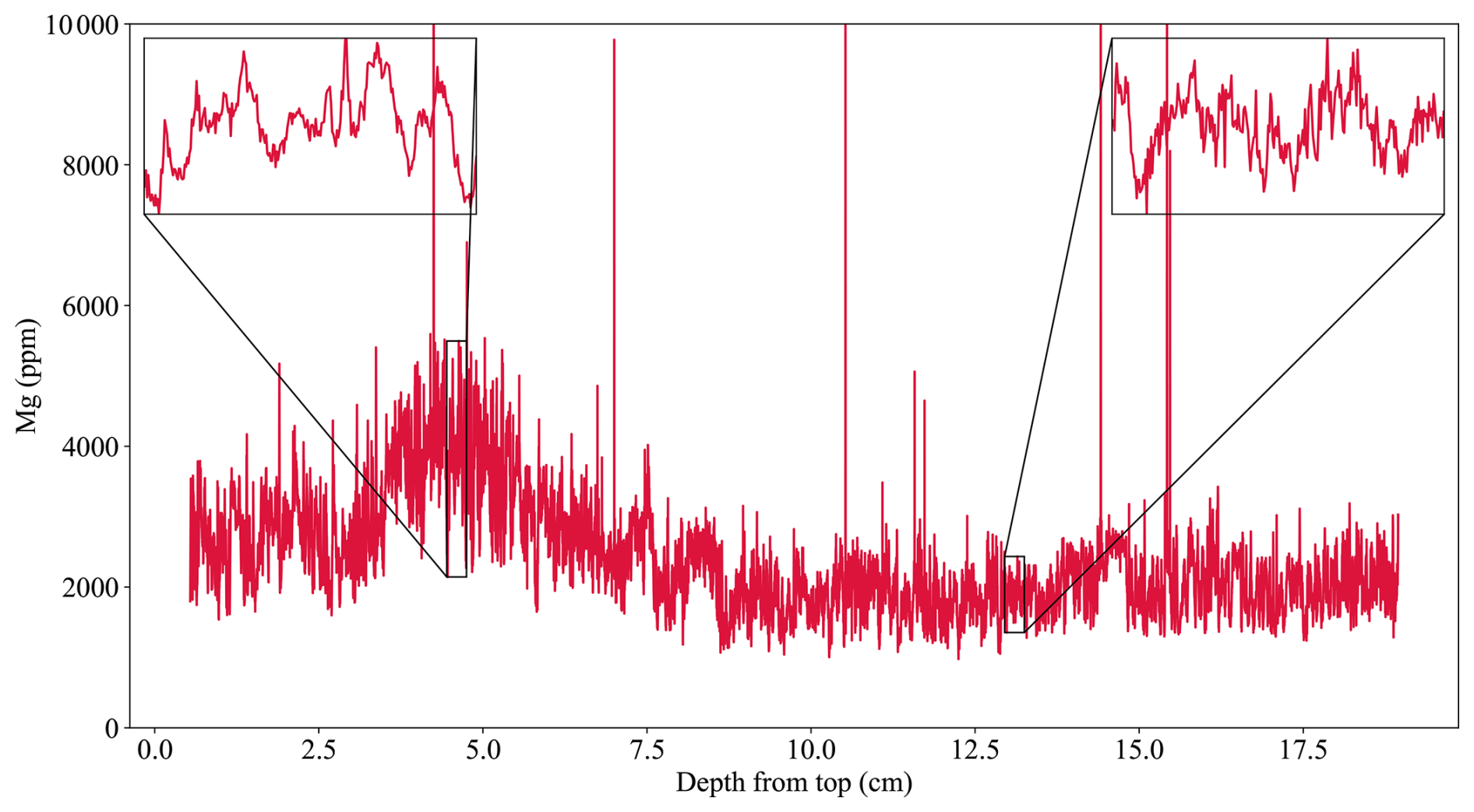
Figure 6 The depth-proxy BER-SWI-13 stalagmite Mg record (red; Forman et al., 2025). The left inset shows an example interval of annual scale cyclicity and the right shows an example of less obvious/absent cyclicity mid-record. Note that the y axis extent is adjusted so that extrema do not reduce figure legibility.

3.1.3 Stalagmite BER-SWI-13

As a final example, we use a speleothem-derived record spanning 564 years (1449–2013 CE) with overall well-developed geochemical cyclicity but with intervals of more ambiguous cyclicity presented in Forman et al. (2025) to test CYCLIM's ability to respond to record gaps (Fig. 6). This stalagmite was collected in 2013 from Leamington Cave in Bermuda and is 19.2 cm tall. The chronology uses radiocarbon dates modelled using the technique presented in Lechleitner et al. (2016) and developed further in Fohlmeister and Lechleitner (2019) to obtain an “average” chronology, which suggests an overall average growth rate of ∼ 0.345 mm yr⁻¹. The 1955 CE bomb spike onset was found at a depth of ∼ 8 mm. A Mg dataset with annual cycles was then used to refine the radiocarbon-based model.

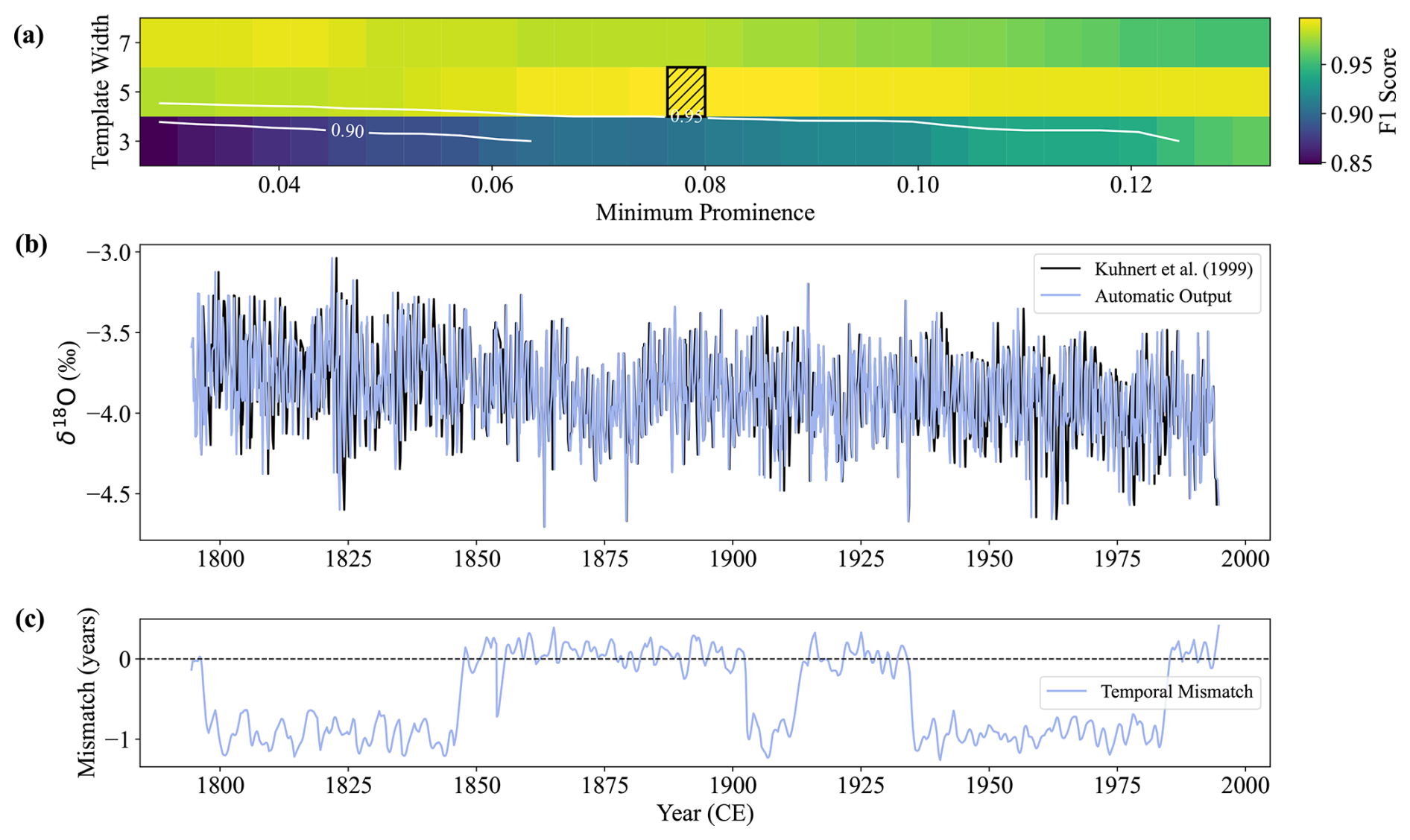
Figure 7 The automatic CYCLIM output for the Houtman Abrolhos Coral record. (a) The sensitivity of the chosen hyperparameters. The black hashed area shows the chosen values of minimum prominence and template width, which are varied by approximately 5 % and 30 %, respectively. Colours correspond to the F1 score between the detected boundaries at a given combination of hyperparameters and that at the black hashed area. F1 score contours of 0.95 and 0.90 are shown. (b) The automatic age-converted output (light blue) shown with the original record (black) presented in Kuhnert et al. (1999). (c) The temporal mismatch: the difference between the published age and the automatic model output at a given point. Positive (negative) values denote older (younger) ages in the published model.

The stalagmite's fast response to rainfall and Mg record's clear dependency on local wind speed variability (ultimately correlated strongly with local temperature) means that the proxy exhibits annual scale cyclicity but with a low signal-to-noise ratio. Magnesium cycle counts were performed by inspection and minima assigned to mid-August, the month of slowest average wind speed. The top ∼ 5.4 mm exhibits pronounced cyclicity loss possibly arising from anthropogenic hydrological changes. Short intervals throughout the record similarly see the cyclicity break down. The original chronology thus models these sections to the radiocarbon average cycle length to maintain chronological accuracy.

3.2 Results

3.2.1 Houtman Abrolhos Coral

The coral record exhibits very clear cyclicity with an average distance of ∼ 1.58 cm, as approximated by spectral analysis. The average distance is approximately 8.11 datapoints and so the algorithm prompts the use of template and tuning windows of 5 and 3 datapoints, respectively. Using the range in y values the starting minimum prominence value is 0.0256 ‰. Visual inspection of the output showed that the minimum prominence criterion was too low, leading to boundary detections due to noise, and so was raised to 0.08 ‰. Sensitivity analysis shows robustness to the choice of minimum prominence (Fig. 7a). The output is sensitive to choice of template width due to the limited number of datapoints per cycle, but the estimate of 5 is likely to be very accurate for the same reason.

The automatic age model achieves a very good match with that published by Kuhnert et al. (1999) with a mean absolute deviation of 0.54 years, 0.3 % of the target's temporal range (Fig. 7b and c). Manual tuning was therefore not required in this case as the algorithm accurately tracked the signal's cyclicity. This is corroborated by the temporal mismatch between the automatic and published age models (Fig. 7c), which jumps between 0 and −1 (minimum = −1.26 years; maximum = 0.41 years) due to the placement of a few cycle boundaries. The sub-annual disparities are the product of differing interpolation methods.

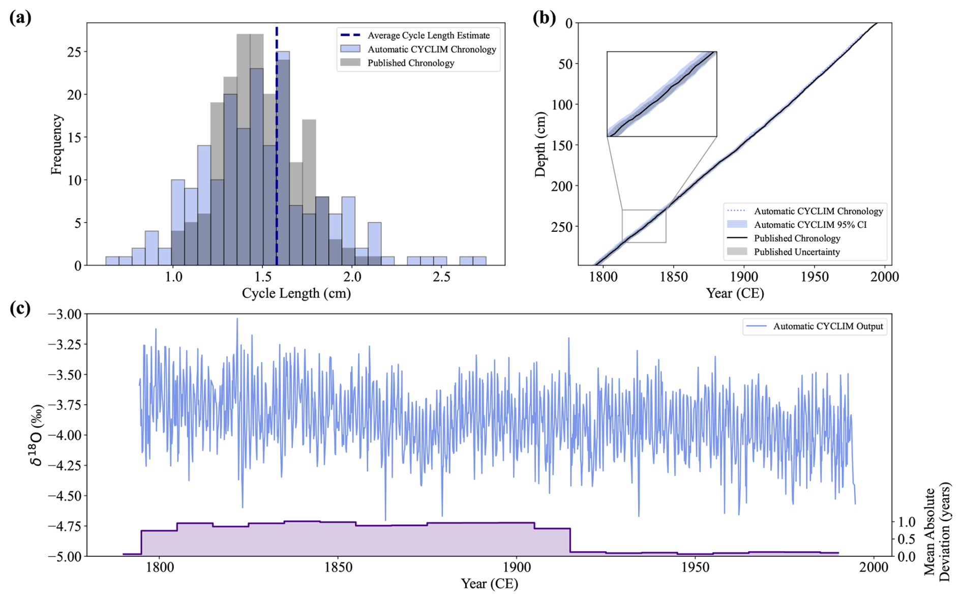
Figure 8 The CYCLIM age model and final output for the Houtman Abrolhos Coral record. (a) Distribution of annual cycle lengths for the automatic (light blue) and published (grey) chronologies. The vertical dashed line shows the average cycle length hyperparameter estimate. (b) The automatic CYCLIM age model (light blue) shown with the published age model (black) presented in Kuhnert et al. (1999), both with their respective uncertainties. (c) The automatic CYCLIM output record (blue) and chronological mismatch with the published record (purple). Mismatches are averaged by decade.

Uncertainty estimation using 1000 random seeds identified the first breakpoint at 13 % noise, prompting 10 000 simulations at this ratio to estimate age errors. The algorithm's 95 % confidence interval agrees with the published uncertainty of ± 1 year per century with an uncertainty of ± 2–3 years at maximum depth (Fig. 8).

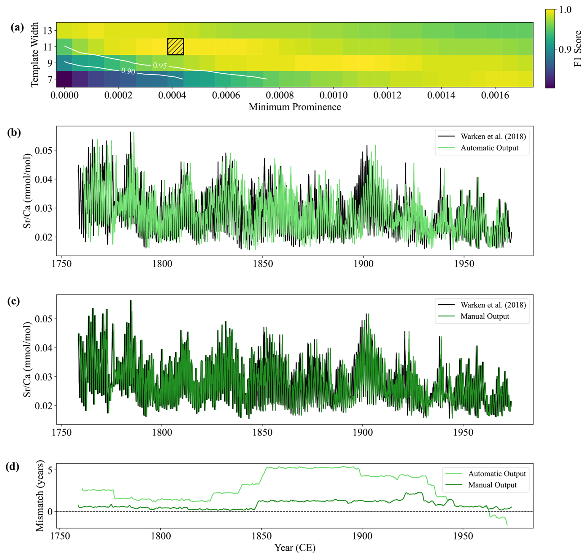
Figure 9 The CYCLIM output for the stalagmite C09-2 record. (a) The sensitivity of the chosen hyperparameters. The black hashed area shows the chosen values of minimum prominence and template width, which are varied by approximately 5 % and 30 %, respectively. Colours correspond to the F1 score between the detected boundaries at a given combination of hyperparameters and that at the black hashed area. F1 score contours of 0.95 and 0.90 are shown. (b) The automatic age-converted output (light green) shown with the original record (black) presented in Warken et al. (2018). (c) The output (dark green) after manual cycle tuning inspection. (d) The temporal mismatch: the difference between the published age and either the automatic (light green) or manual (dark green) model outputs at a given point. Positive (negative) values denote older (younger) ages in the published model.

3.2.2 Stalagmite C09-2

The C09-2 stalagmite record has a more variable cycle length and contains more noise (Warken et al., 2018), providing an opportunity to test the algorithm's versatility. Spectral analysis suggests the average annual cycle length is approximately 0.292 mm, which equates to 23.6 datapoints. The default hyperparameter choices thus become 11 and 5 points for the template width and tuning window, respectively. Additionally, the default minimum prominence corresponds to 0.0007 mmol mol⁻¹. Visual inspection suggests this default setting was too high as some cycle boundaries are being missed and so was lowered to 0.0004 mmol mol⁻¹. Sensitivity analysis shows both the choice of template width and minimum prominence are robust but is approaching the lower end of the stable region (Fig. 9a). This is primarily due to the minimum prominence approaching 0 mmol mol⁻¹.

The automatic output exhibits excellent agreement with the record published in Warken et al. (2018) with a mean absolute deviation of 2.91 years, 1.35 % of the target's temporal range (Fig. 9b and d). However, the algorithm still misses some cycle boundaries due to their comparatively low amplitude and so the output required tuning. This systematic error is shown by the temporal mismatch (Fig. 9d), which shows a steady rise to a maximum of 5.42 years in the middle of the record which is then compensated by an overcount in the oldest part of the record. Manual inspection found 7 erroneous cycles and resulted in the addition of 12 cycles, meaning the automatic output found 94.4 % of the cycles and achieved an F1 score of 0.96. The tuned record has a maximum absolute mismatch of 2.31 years (mean absolute deviation = 0.79 years) showing strong agreement with the published record (Fig. 9c and d).

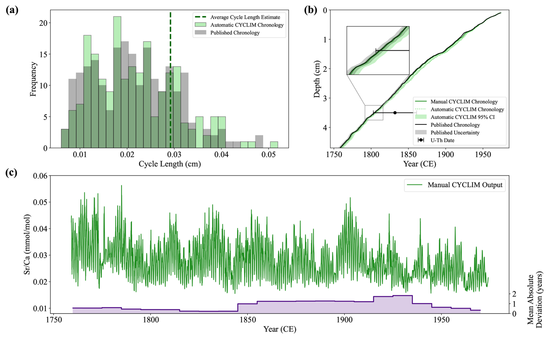
Figure 10 The CYCLIM age models and manually tuned output for the stalagmite C09-2 record. (a) Distribution of annual cycle lengths for the automatic (light green) and published (grey) chronologies. The vertical dashed line shows the average cycle length hyperparameter estimate. (b) The CYCLIM age models (automatic – light green; manual – dark green) shown with the published age model (black) presented in Warken et al. (2018), with their respective uncertainties. (c) The manual CYCLIM output record (green) and chronological mismatch with the published record (purple). Mismatches are averaged by decade.

Uncertainty quantification used 1000 random seeds and 10 000 simulations at a noise level of 7 %. Simulations were constrained by the U-Th date uncertainties and led to the rejection of 232 realisations. Algorithmic uncertainties broadly follow those presented in the Warken et al. (2018) with a 95 % algorithmic uncertainty of approximately ± 3 years at maximum depth in both age models. Though, due to the systematic nature of the tuning, the manual and published age models plot outside of the algorithmic uncertainty, but the uncertainties do overlap (Fig. 10b).

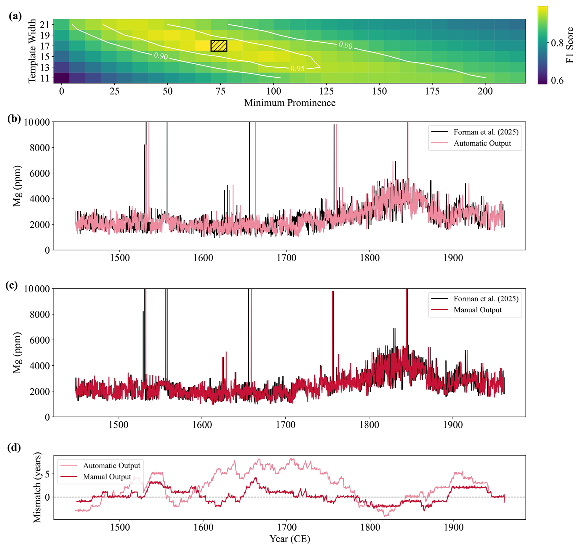
Figure 11 The CYCLIM output for the stalagmite BER-SWI-13 record. (a) The sensitivity of the chosen hyperparameters. The black hashed area shows the chosen values of minimum prominence and template width, which are varied by approximately 5 % and 30 %, respectively. Colours correspond to the F1 score between the detected boundaries at a given combination of hyperparameters and that at the black hashed area. F1 score contours of 0.95 and 0.90 are shown. (b) The automatic age-converted output (pink) shown with the original record (black) presented in Forman et al. (2025). (b) The output (red) after manual cycle tuning inspection. (d) The temporal mismatch: the difference between the published age and either the automatic (pink) or manual (red) model outputs at a given point. Positive (negative) values denote older (younger) ages in the published model.

3.2.3 Stalagmite BER-SWI-13

This final dataset assesses the algorithm's ability to respond to sections with very weak and ambiguous cyclicity. Radiocarbon modelling of stalagmite BER-SWI-13's growth suggests a mean cycle length of approximately 0.345 mm which corresponds to ∼ 33.6 datapoints. The template width and tuning window therefore become 17 and 9 points, respectively. The tool prompts the use of 71.8 ppm for the minimum prominence criterion. Sensitivity analysis shows that the output is sensitive to both the choice of template width and minimum prominence (Fig. 11a), highlighting the output will need probably require manual tuning. Additionally, the top ∼ 5.4 mm is subjected to complete cyclicity loss and so the original paper models this section so that the top matches the collection year, but due to the substantial chronological uncertainty over this interval, this section is left out of the input.

The automatic age model shows broad agreement with the original record achieving an overall mean absolute deviation of 3.24 years (0.63 % of the target's temporal range) (Fig. 11b and d). There are small over/under-counts at ages younger than 1800 CE, but a serial undercount emerges thereafter reaching a maximum offset of 8.35 years, before being counteracted by a subsequent overcount. The trend suggests that in areas of ambiguous cyclicity, the detection criteria of the algorithm is not aligning well with that of manual inspection. Given the noise level of this record, this degree of misalignment is within expected uncertainties and so the automatic output could be used without tuning. However, because of the complexity of the proxy signal, cycle boundaries were inspected and adjusted following inspection. Manual tuning removed 35 and added 33 cycles, meaning the automatic output found 93.6 % of the cycles and achieved an F1 score of 0.93. The tuned record has a maximum absolute mismatch of 4.18 years (mean absolute deviation = 1.10 years) showing strong agreement with the published record.

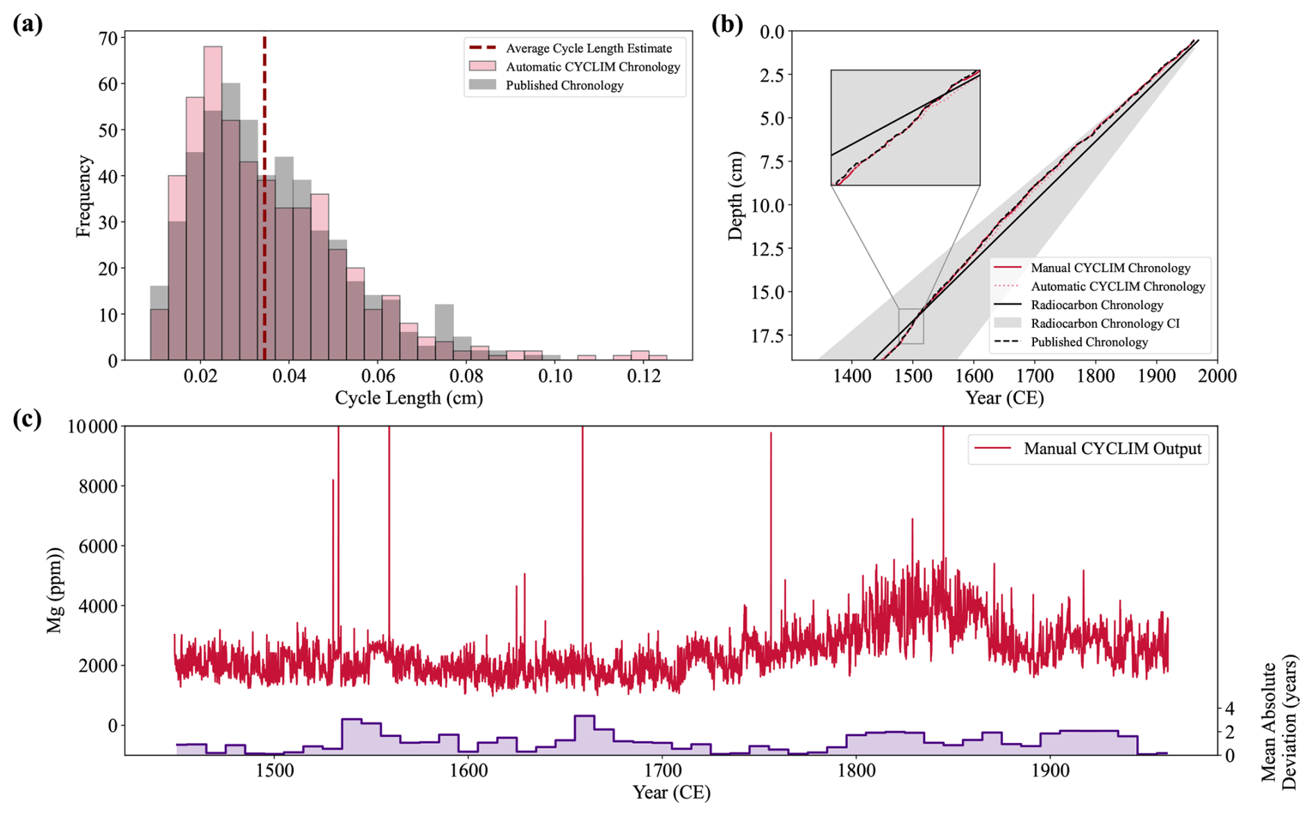
Figure 12 The CYCLIM age models and manually tuned output for the stalagmite BER-SWI-13 record. (a) Distribution of annual cycle lengths for the automatic (pink) and published (grey) chronologies. The vertical dashed line shows the average cycle length hyperparameter estimate. (b) The CYCLIM age models (automatic – pink; manual – red), shown with the published age model (black) and the radiocarbon carbon chronology with 2σ uncertainties presented in Forman et al. (2025). (c) The manual CYCLIM output record (red) and chronological mismatch with the published record (purple). Mismatches are averaged by decade.

Uncertainty modelling with 1000 random seeds and 10 000 simulations was attempted, but the breakpoint could not be determined, and so estimates were not obtained. Because of the record's signal quality and hyperparameter sensitivity, algorithm accuracy degraded too fast and linearly to increasing noise for the first breakpoint to occur at a noise level > 2 %. However, both the automatic and manual age models plot within the published radiocarbon chronology confidence interval (Fig. 12b).

4 Discussion

4.1 Manual vs. Automated Cycle Counting

The automatic output has three main advantages over counting by inspection: (1) it returns results much faster; (2) the results are reproducible with the same inputs; and (3) it reduces subjectivity. Although manual counting is more flexible and able to adapt to changes in growth rate or noise levels, it risks false positives given the position of boundaries under these conditions often becomes subjective. Similarly, if the depth-proxy signal has been compared to previous records prior to age-model development, then the inspector risks incorporating confirmation bias into the cycle count. One of the underlying assumptions of the results is that the published age models are correct; however, there is inherent uncertainty with these chronologies too. Thus, the comparison statistics gauge the accuracy of the output, but once discrepancies fall within the original age model's uncertainty, further alignment may become erroneous.

Whether to tune to automatic output thus depends on the record's structure. If the proxy shows clear, consistent cyclicity then it could be argued that the automated output is accurate, and tuning may introduce false precision. Conversely, if the waveform changes shape substantially throughout the record (e.g., due to fluctuating growth rates or noise levels), the Gaussian template may not reliably amplify annual scale cyclicity, risking systematic bias. In this case, the automated output and its accompanying uncertainties may be inaccurate and thus require manual tuning.

It is important to note that only the automatic output yields quantified algorithmic uncertainty. Manual tuning forfeits this benefit, and introduces its own uncertainty tied to the inspector's judgements. Thus, when the algorithm can only provide a basis to count from due to systematic error, the user must manually tune the output. However, when the cyclicity is sufficiently predictable to yield an accurate chronology, whether to tune the output becomes a choice. A user may decide to report both an accurate automated chronology with uncertainty and show the precise, manually tuned age model for comparison. This way small potential errors made by the algorithm can be corrected whilst also retaining the benefits of quantified uncertainty and transparency of an automated count. Regardless of the signal's clarity, any automated output should always be quality-checked to ensure cyclicity is being correctly tracked.

4.2 CYCLIM Performance

The CYCLIM algorithm extracts the positions of cycle boundaries from the three examples both accurately and quickly via an automated matched filtering technique, achieving close approximations of the original chronologies. Across the three examples the temporal offsets ranged from −4.22 to 8.35 years with an average mean absolute deviation of 2.23 years before correction. While the accuracy does depend on the choice of hyperparameters, only two require estimation. Because the average cycle length estimate is derived from other methods (e.g., approximated from a U-Th age model or by spectral analysis), this is a fixed value leaving only the minimum prominence at the discretion of the user to change. The automatic minimum prominence value provides a viable starting place but due to the range in proxy signals it will likely need to modification. Users can easily override this with a better estimate obtained from inspection of the algorithm's output. Thus, the matched filtering approach is robust and can greatly speed up the cycle counting process by providing a first-pass count for the user to refine.

Post-analysis users should check and refine the automatic output in the cycle tuning stage to mitigate issues such as: (1) overcounting resulting from gap treatment; (2) undercounting due to low signal-to-noise; (3) a change in average cycle width hindering hyperparameter effectiveness; and (4) erroneous hyperparameter choices. Tuning found an average 5.07 % erroneous detection error and 6.01 % missed detection error, meaning that cycle counting within CYCLIM was an order of magnitude faster for the two examples that required this step. The tuned results follow the original chronologies very closely and further running could yield a perfect match. However, to ensure a fair test, tuning was conducted independently and without back-calculation of cycle boundaries using the published chronology. Thus, whereas the outputs are not perfect reflections of the originals, they are within the expected counting errors, hence demonstrating the efficacy of the CYCLIM tool.

The two-stage semi-automated approach generates high-precision cycle counts within the errors expected of count reproducibility and could be applied to a wide variety of archives, provided the assumptions hold. CYCLIM could have several potential uses besides simply generating a chronology, for example: (1) reporting an objective cycle count with uncertainties (i.e., the algorithm output) before correction; (2) easily running multiple counts to test reproducibility; and (3) reporting an objective count before then running multiple corrections to develop an average age model.

5 Conclusions

Here we present a new semi-automated Python-based application (CYCLIM) for deriving chronologies from annual-scale cycle counting. The algorithm performs an initial cycle count using matched filtering, after which the user may inspect and refine the output by removing false detections and/or adding in missed cycles. The method accommodates multiple forms of chronological constrains, such as an anchor point and other tie points. Based on the testing presented here, CYCLIM generates quick and accurate automatic counts, often within counting errors and an order of magnitude faster than by inspection. It provides a reliable first-pass model while also allowing users to correct the output where needed within a user-friendly GUI. When the signal is sufficiently robust to the noise-based perturbation approach, CYCLIM successfully quantifies algorithmic uncertainty, yielding confidence intervals consistent with published age errors and highlighting where cyclicity becomes more subjective. This framework thus promotes rapid, reproducible, and transparent cycle counting and can serve as a basis for reporting objective and subjective cycle boundaries, as well as developing average manual age models.