Climate and stratospheric ozone during the mid-Holocene and Last Interglacial simulated by MRI-ESM2.0

The climates of the mid-Holocene (MH) and Last Interglacial (LIG) are characterised by warm periods caused by astronomical forcing and climate feedback. One potential feedback is variation in the stratospheric ozone, the influence of which would extend down to the troposphere, potentially affecting the climate. However, little is known about the role of changes in the stratospheric ozone during past warm interglacial periods. Here, we employ MRI-ESM2.0, an Earth system model with an interactive ozone model, and simulate the climate and atmospheric ozone during the MH and LIG. We show that the vertical and seasonal changes of stratospheric ozone in the LIG exhibited a stronger variation in the stratospheric ozone compared to that in the MH, indicating that both obliquity and precession forcings affect the stratospheric ozone distributions. We further show that ozone feedbacks decrease the surface air temperature by ∼ 0.35 and ∼ 0.25 K in the high-latitude regions of the northern hemisphere in MH and LIG, respectively, while the impact on the zonal mean surface air temperature around Antarctica is small. This is the opposite of the previous finding that implies the importance of ozone in southern hemisphere climates, indicating the need for further assessment of how dynamic ozone variations affect climate and atmospheric structures during past warm interglacial periods using multiple Earth system models.

1 Introduction

Investigation of past interglacials can provide fundamental knowledge of feedback mechanisms that interact between the atmosphere, sea ice, and land surface under warmer climatic conditions (Otto-Bliesner et al., 2021). The climates of the mid-Holocene (MH; 6 ka) and the Last Interglacial (LIG; 127 ka) are characterised by warm and humid land climate conditions, which would be attributed primarily to the different configurations of astronomical forcing (i.e., obliquity, precession, and eccentricity) that result in latitudinal and seasonal changes in insolation (Fig. 1) (Braconnot et al., 2007, 2012; Otto-Bliesner et al., 2017, 2021). Paleoclimate proxy data indicate that the global mean surface air temperature was ∼ 0.7 and ∼ 1.3 K higher than the preindustrial (PI) conditions in the MH and LIG, respectively (Turney and Jones, 2010; Marcott et al., 2013; Fischer et al., 2018; Kaufman et al., 2020b, a; Kaufman and Broadman 2023). The warming is especially enhanced over high-latitude regions, possibly reflecting the amplification by feedback mechanisms such as sea-ice changes over the Arctic Ocean and vegetation feedback over land areas of the Northern Hemisphere (Otto-Bliesner et al., 2006; Kageyama et al., 2021; O'ishi and Abe-Ouchi, 2011; O'ishi et al., 2021). However, many climate models do not simulate the higher global annual mean surface air temperature inferred from the paleoclimate proxy during the MH and LIG (Masson-Delmotte et al., 2013; Otto-Bliesner et al., 2013; Liu et al., 2014; Brierley et al., 2020; Kaufman and Broadman 2023). The cause of this discrepancy has been vigorously debated (Liu et al., 2014, 2018; Hopcroft and Valdes, 2019; Park et al., 2019; Bova et al., 2021; Zhang and Chen, 2021; Thompson et al., 2022; Laepple et al., 2022; Kaufman and Broadman, 2023), indicating that high-latitude processes over land and ocean are critical for further understanding the climate warming during the past interglacials. Indeed, the minimal extent of sea ice in both Arctic and Antarctic regions would have been smaller than in the PI condition in the MH and LIG owing to the different insolation forcing and associated internal feedbacks (Yoshimori and Suzuki, 2019; Brierley et al., 2020; Otto-Bliesner et al., 2020; Guarino et al., 2020; Diamond et al., 2021; Kageyama et al., 2021; Sime et al., 2023; Chadwick et al., 2023; Yeung et al., 2024; Gao et al., 2025). Particularly, northern hemisphere sea ice may have completely melted seasonally during the LIG, which has a profound impact on the climate (Guarino et al., 2020; Diamond et al., 2021; Sime et al., 2023).

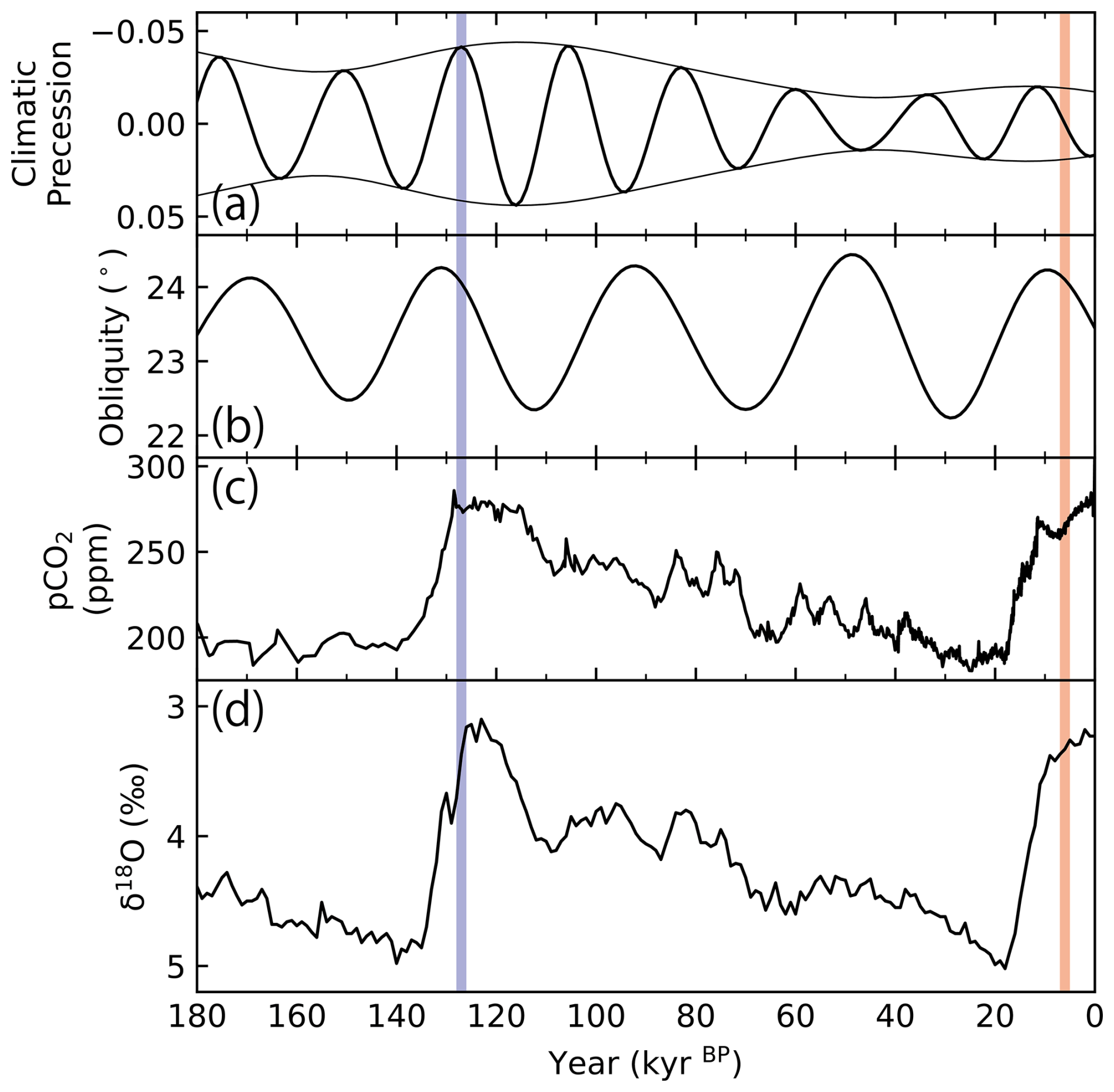
Figure 1 Changes in (a) eccentricity (envelope curve) and climatic precession (Berger and Loutre, 1991), (b) obliquity of the Earth (Berger and Loutre, 1991), (c) atmospheric pCO₂ (Bereiter et al., 2015), and (d) stacked oxygen isotope signatures (Lisiecki and Raymo, 2005) for the last 180 kyr.

One possible factor that can affect the high latitudes is stratospheric ozone-climate feedbacks (Thompson and Wallace, 2000; Noda et al., 2017). It has been shown that changes in the ozone hole around the South Pole (SP) during the late 20th century affect the climate around Antarctica by changing the atmospheric structure and circulation patterns over those regions. Particularly, the depletion of the stratospheric ozone around the SP cools the stratosphere and strengthens the westerly jet and the positive Southern Annular Mode (Thompson and Wallace, 2000; Noda et al., 2017). This has been pointed out to further affect the distribution of sea ice around Antarctica because the changes in jet strength affect the Ekman transport in the Southern Ocean (SO) and the warming of the surface ocean, while the plausibility and impact on the historical period remains still uncertain (Sigmond and Fyfe, 2010, 2014; Bitz and Polvani, 2012; Ferreira et al., 2015; Smith et al., 2012; Noda et al., 2017; Langematz et al., 2018). Despite the uncertainty regarding the impact of the mechanism caused by the human-induced ozone depletion in the late 20th century, a similar ozone-climate mechanism may have worked in response to different astronomical forcing during past interglacials (Noda et al., 2017). A previous study employed the Earth system model MRI-ESM1, which couples an interactive ozone model, to estimate the response of the ozone layer during the MH (Noda et al., 2017). This study showed that the positive ozone anomaly in the upper stratosphere around the South Pole during the austral summer of the MH would propagate to the lower stratosphere in the austral winter. This anomaly would increase the air temperature and weaken the southern westerly jet. They further suggested that it may contribute to the retreat of sea ice in the Southern Ocean during the MH. They showed that the positive ozone anomaly with a maximum value of ∼ 0.2 ppm in the stratosphere would be caused by the different astronomical forcing during the MH. They further showed that this would lead to the annual zonal mean surface air temperature anomaly of up to +1.7 K around the South Pole. Thus, consideration of the interactive ozone layer in climate models would potentially affect the estimated climate state near the southern polar region. Particularly, the effect of ozone distribution changes may strengthen further and enhance the climate change during the LIG owing to the effect of precession forcing under the high eccentricity during this period (Fig. 1), which may have contributed to the warming around Antarctica during the LIG. In the latest Paleoclimate Modelling Intercomparison Project (PMIP4), however, only one model, Meteorological Research Institute Earth System Model 2.0 (MRI-ESM2.0) (Yukimoto et al., 2019), couples an interactive ozone chemistry model. While several studies have investigated the role of changes in ozone distribution during the Last Glacial Maximum (Rind et al., 2009; Murray et al., 2014; Noda et al., 2018; Wang et al., 2020, 2022), the validity of the role of ozone layer changes in response to different astronomical forcings during the MH pointed out by Noda et al. (2017) and its impact on the LIG climate system remains ambiguous.

In this study, we first test the response of the stratospheric ozone and its impact on climate during the MH using a state-of-the-art Earth system model. We then investigate the response of stratospheric ozone in both MH and LIG to show the impact of different astronomical forcing. For this purpose, we employed MRI-ESM2.0 and simulated the climate and the atmospheric ozone distribution under the MH and LIG conditions. Here, we discuss the atmospheric structure and circulation pattern with a specific focus on high-latitude regions in the Southern Hemisphere, the ozone distribution changes during the MH and LIG, and their impact on the climate and atmospheric circulation.

2 Method

In this study, we employed MRI-ESM2.0 (Yukimoto et al., 2019), which couples the atmospheric general circulation model (AGCM) with land processes MRI-AGCM3.5, the aerosol model MASINGAR mk-2r4c (Tanaka et al., 2003), the atmospheric chemistry climate model MRI-CCM2.1 (Deushi and Shibata, 2011), and the ocean and sea ice model MRI.COMv4. The horizontal resolutions of the model grid are TL159 (∼ 120 km) for MRI-AGCM3.5, TL95 (∼ 180 km) for MASINGAR mk-2r4c, and T42 (∼ 280 km) for MRI-CCM 2.1 (Yukimoto et al., 2019). The number of vertical layers of the AGCM, aerosol, and ozone models is 80. The MH conditions were previously calculated for PMIP4, but the LIG conditions have not been calculated.

Table 1 List of numerical experiments conducted in this study.

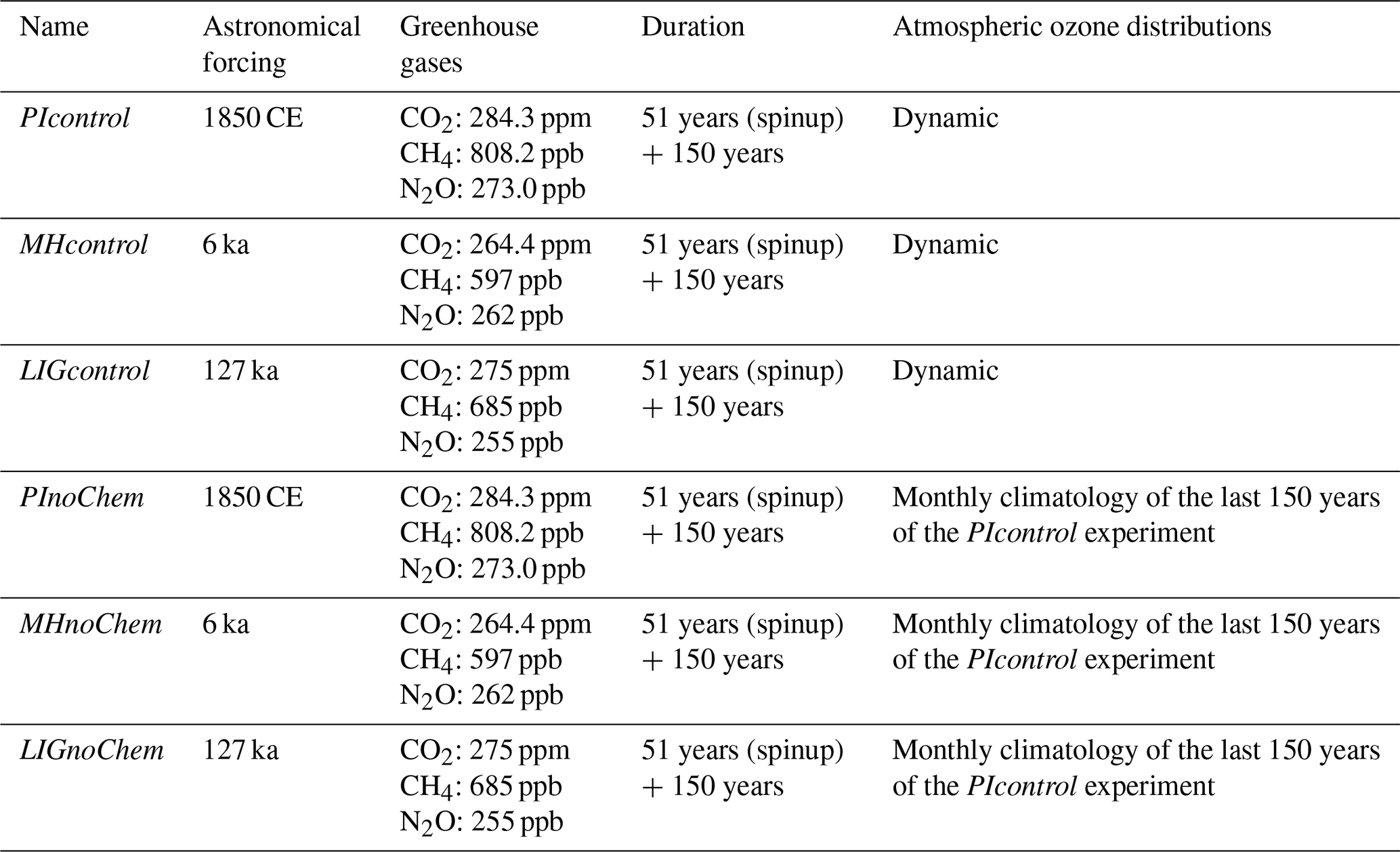
We conducted the simulation using MRI-ESM2.0 under the PI conditions (Eyring et al., 2016; Menary et al., 2018) for 201 model years starting from the well-spun-up PI conditions submitted to CMIP6 to achieve a new steady state reflecting the minor improvement of the model (PIcontrol) (Table 1). We also conducted simulations under the MH and LIG conditions for 201 model years (MHcontrol and LIGcontrol, respectively) (Table 1), starting from the MH simulation submitted to PMIP4. In these calculations, the last 150 years were used for the analysis and the first 51 years were omitted as a spin-up period. We note that this spin-up period is relatively short compared to many of the PMIP4 experiments for these periods, and only two models have a spin-up period of 50 years (e.g., Kageyama et al., 2021). For this reason, the processes with long timescales, such as the oceanic circulation, would not have reached a steady state. Nevertheless, the response of total ozone during the MH and LIG had sufficiently reached a steady state after the spin-up period, so we consider this would not change our main conclusion. These calculations were conducted following the PMIP4 protocol (Otto-Bliesner et al., 2017). To elucidate the effect of the changes in the ozone distributions in the atmosphere, we also ran the model under the PI, MH, and LIG conditions using the monthly ozone climatology of the last 150 years of the calculation for the PI conditions (PInochem, MHnochem, and LIGnochem, respectively) (Table 1). These calculations were conducted for 201 years, and the last 150 years were analysed. The calendar adjustment was conducted in all the monthly output data for MH and LIG conditions outputs to consider the changes in the length of months (Bartlein and Shafer, 2019).

3 Results

3.1 Stratospheric ozone under the MH and LIG conditions

The latitudinal-vertical plot of the zonal-mean ozone concentration anomaly for the MH and LIG conditions from the PI condition is shown in Fig. 2a. For the case of the MH, the ozone concentration is higher compared to PI in the lower stratosphere at low-latitude regions and near the South Pole, while it is lower in the upper stratosphere at low-latitude regions and near the North Pole. As a result, the 150-year mean value of total ozone is 314.7 DU, which is slightly lower than the PI value (315.4 DU). For the case of the LIG, on the other hand, the 150-year mean value of total ozone is 316.7 DU, which is slightly higher than in the PI. This is related to the positive anomaly in ozone concentration in broad regions of the lower stratosphere (Fig. 2b). These anomalies would be primarily associated with the different astronomical forcing during the MH and LIG. The latitudinal and seasonal changes in the top-of-atmosphere insolation anomaly and air temperature and the ozone concentration anomalies in the upper stratosphere (3 hPa) are shown in Fig. 3. In both the MH and LIG conditions, the changes in the temperature in the upper stratosphere correlate positively with the changes in the top-of-atmosphere (TOA) insolation owing to the shortwave ozone heating (Fig. 3a, b, c, and d). The ozone concentration in the upper stratosphere, on the other hand, correlates negatively with the insolation and temperature anomalies (Fig. 3e and f). The inverse correlation between the air temperature and ozone concentration is explained by the changes in the steady state of the chemical reactions in the Chapman cycle (Chapman, 1930; Noda et al., 2017) because a higher temperature promotes the following ozone destruction reaction:

$$\begin{array}{}\text{(R1)}& {\mathrm{O}}_{\mathrm{3}}+\mathrm{O}\to \mathrm{2}{\mathrm{O}}_{\mathrm{2}}.\end{array}$$

This would lead to the promotion of the other reactions in the Chapman cycle:

$$\begin{array}{}\text{(R2)}& {\displaystyle }{\mathrm{O}}_{\mathrm{2}}+hv\to \mathrm{2}\mathrm{O},\text{(R3)}& {\displaystyle }{\mathrm{O}}_{\mathrm{2}}+\mathrm{O}+\mathrm{M}\to {\mathrm{O}}_{\mathrm{3}}+\mathrm{M},\text{(R4)}& {\displaystyle }{\mathrm{O}}_{\mathrm{3}}+hv\to {\mathrm{O}}_{\mathrm{2}}+\mathrm{O}.\end{array}$$

Although the insolation anomaly in the MH and LIG would also affect the photochemical reaction rates of Reactions (R2) and (R4), the negative correlation indicates that the temperature effect of Reaction (R1) would dominate the behavior of stratospheric ozone anomalies in the MH and LIG. For this reason, the different astronomical forcing in the MH and LIG results in a strong seasonal cycle of the ozone concentration in the upper stratosphere. The decrease in the ozone concentration would work in the direction of suppressing the warming in the upper stratosphere, but the temperature increases because of the increase in shortwave radiation during austral winter in the MH and LIG. In the case of the MH conditions, the ozone concentration anomaly in the upper stratosphere becomes negative during May and turns positive during January (Fig. 3e). In the case of the LIG conditions, the overall pattern of the seasonal response of temperature and ozone concentration in the upper stratosphere is similar to that in the MH conditions, but the signal is stronger in the LIG compared to that in the MH. The notable difference in the LIG is that the ozone concentration anomaly in the upper stratosphere turns negative during March and April and positive during October and November (Fig. 3f), following the different insolation anomaly associated with variations in the precession (Fig. 3b).

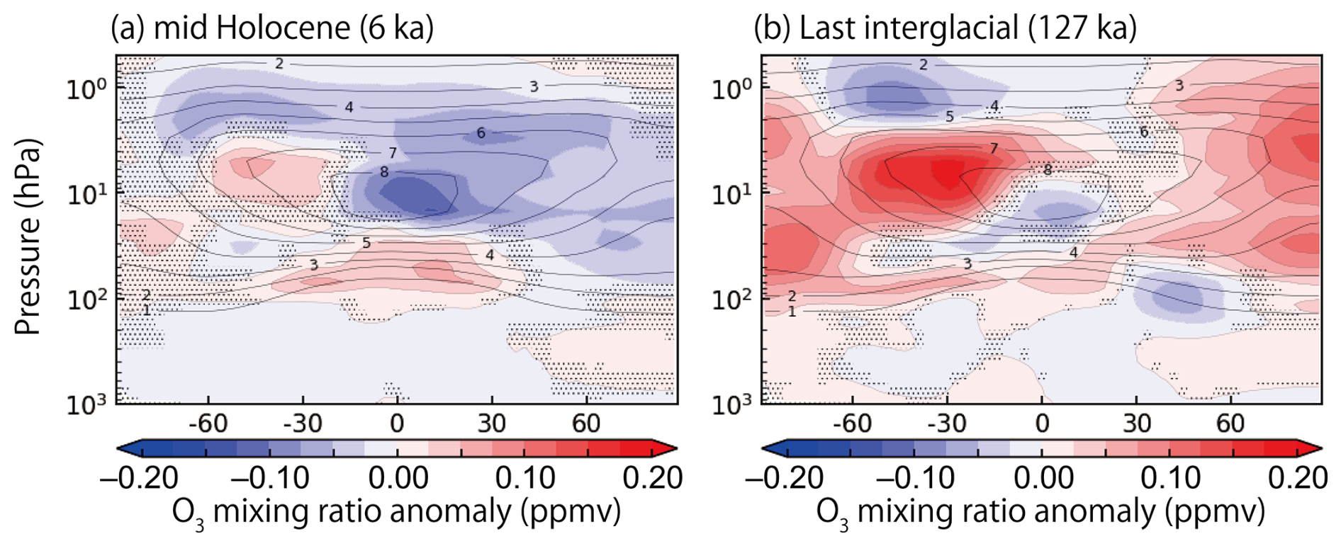
Figure 2 Zonal and annual mean ozone anomaly relative to the preindustrial (PI) condition in the (a) MH (MHcontrol–PIcontrol) and (b) LIG (LIGcontrol–PIcontrol). The contour represents the zonal and annual mean ozone concentration in the MH and LIG, respectively. The dotted area represents the region where 95 % confidence interval was not achieved.

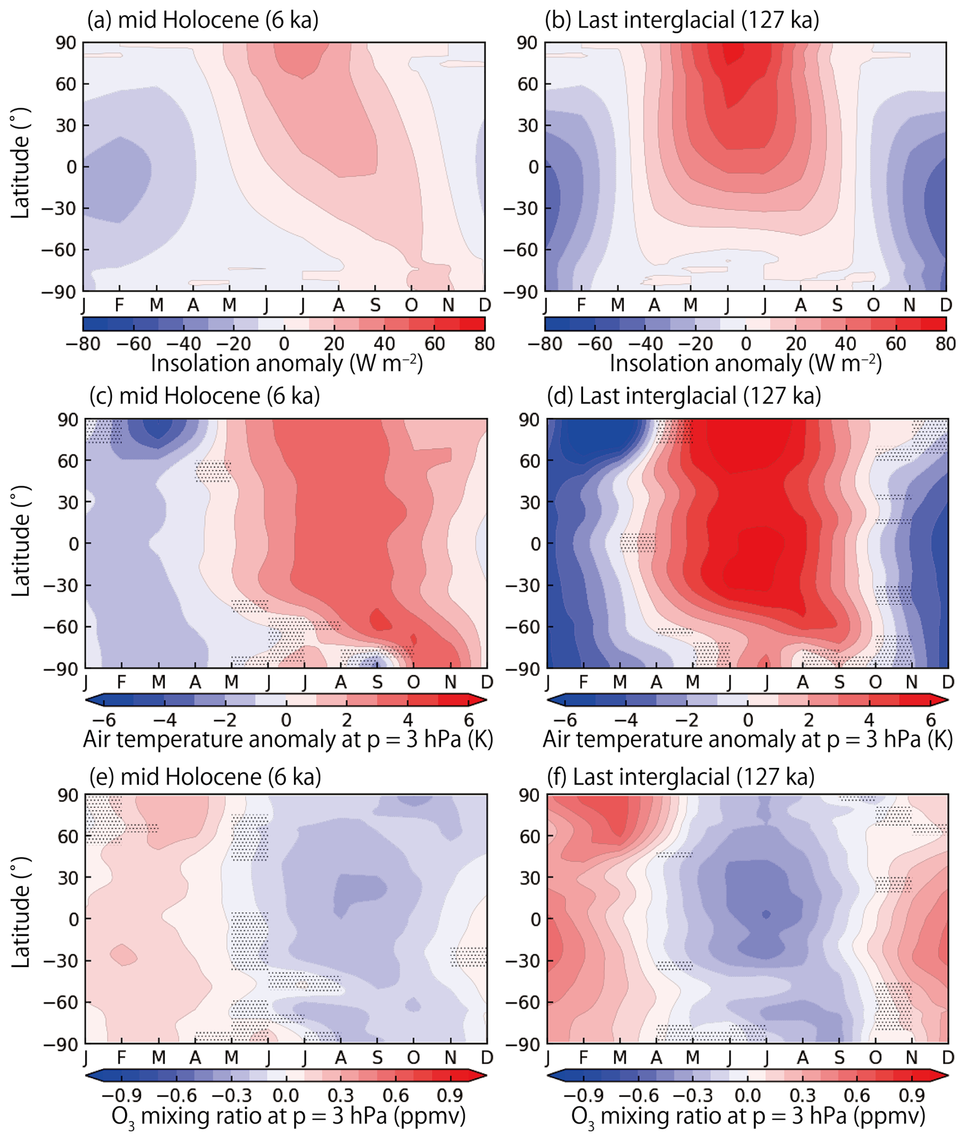
Figure 3 Top-of-atmosphere insolation anomaly (a–b), air temperature anomaly at a pressure level of 3 hPa (c–d), and ozone concentration anomaly at a pressure level of 3 hPa (e–f) for the mid-Holocene (MH) condition (MHcontrol–PIcontrol) (a, c, e) and the Last Interglacial condition (LIGcontrol–PIcontrol) (b, d, f), relative to the preindustrial condition. The dotted area in (c–f) represents the region where 95 % confidence interval was not achieved.

The pattern of the temperature and ozone anomalies in the upper stratosphere (Fig. 3c and e) in the MH simulated by our model is broadly consistent with the results of a previous study using the former version of MRI-ESM under the MH conditions (Noda et al., 2017). This would indicate a robust response of the ozone concentration to the different astronomical forcings during the MH.

The simulated zonal and annual mean air temperature is shown in Fig. 4a–b. Both in the MH and LIG, the temperature increased compared with the PI broadly in the stratosphere. This reflects the seasonal warming caused by the astronomical forcing in Fig. 3c and d. The tropospheric air temperature, on the other hand, decreases especially in the tropics in both MH and LIG. Specifically, the tropospheric air temperature increases by 0.5–1 K in the troposphere of the mid- and high-latitude regions in the northern hemisphere in the LIG. Part of these anomalies may be associated with the changes in the ozone distributions. In Fig. 4c and d, the ozone-induced changes in the zonal and annual-mean air temperature for the MH and LIG are shown, respectively. In the MH, the change in ozone distribution increases the temperature in the lower stratosphere in the tropics, while a significant signal was not observed in the troposphere in the MH. In the LIG, on the other hand, a significant signal was observed in the upper troposphere of the high-latitude regions of both hemispheres.

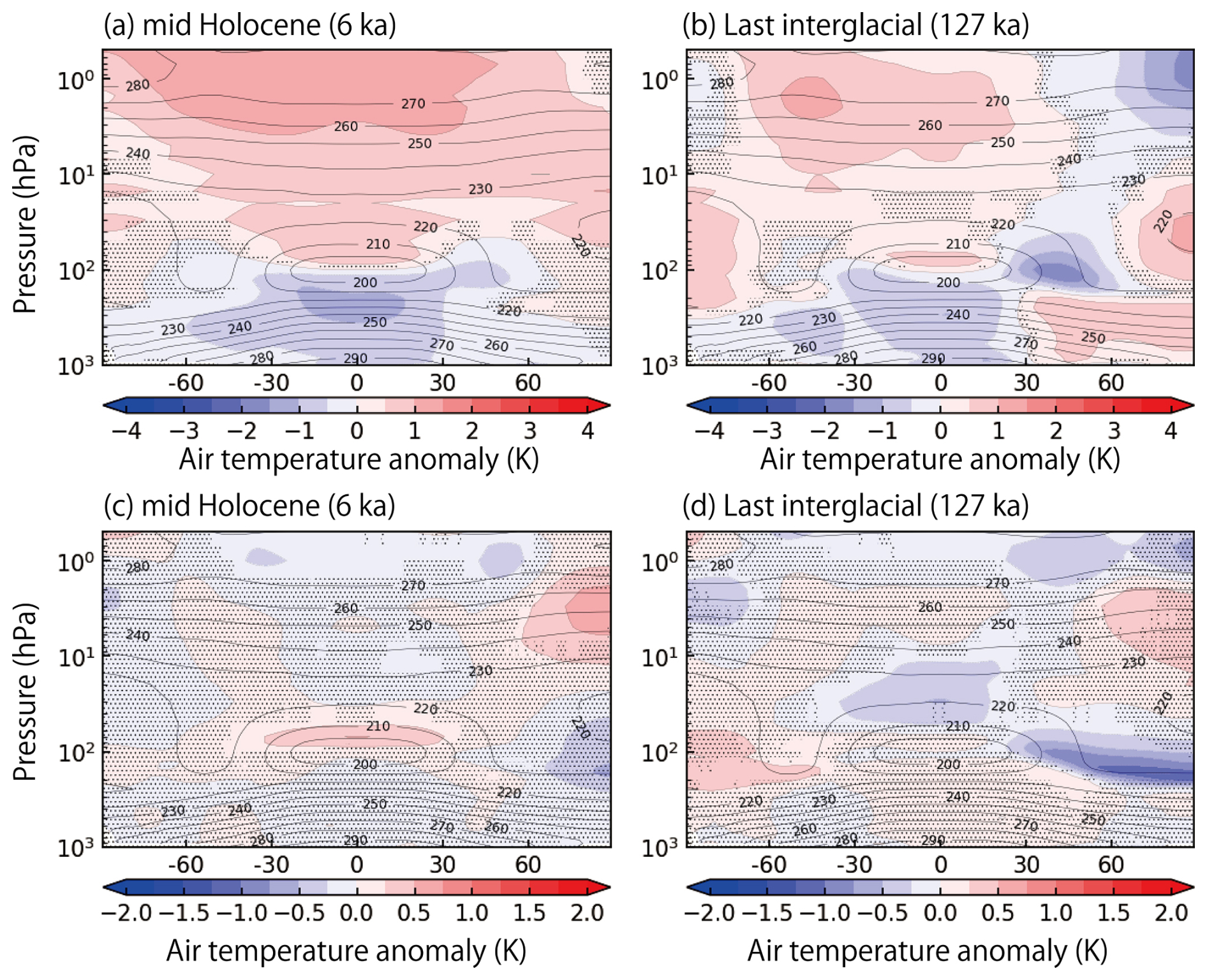
Figure 4 Zonal and annual mean air temperature anomaly relative to the preindustrial (PI) condition in the (a) MH (MHcontrol–PIcontrol) and (b) LIG (LIGcontrol–PIcontrol). Zonal and annual mean ozone-induced air temperature anomaly relative to the preindustrial (PI) condition in the (c) MH (MHcontrol–PIcontrol–MHnoChem + PInoChem) and (d) LIG (LIGcontrol–PIcontrol–LIGnoChem + PInoChem). The contour represents the zonal and annual mean ozone concentration in the MH and LIG, respectively. The dotted area represents the region where 95 % confidence interval was not achieved.

The seasonal and vertical distributions of air temperature and ozone anomalies in the tropic regions (between 15° S and 15° N) in the MH and LIG are shown in Fig. 5a–d. In both periods, the seasonal variations in stratospheric air temperature and ozone concentration, caused by different astronomical forcing, are widespread in the upper stratosphere, both in the MH and LIG. In the lower stratosphere, on the other hand, a positive ozone anomaly was seen when the ozone anomaly in the stratosphere was negative in both MH and LIG. This would be because more ultraviolet radiation reaches the lower stratosphere due to the low ozone concentration in the upper stratosphere, leading to the positive anomaly of ozone concentration in the troposphere (Fig. 5c and d).

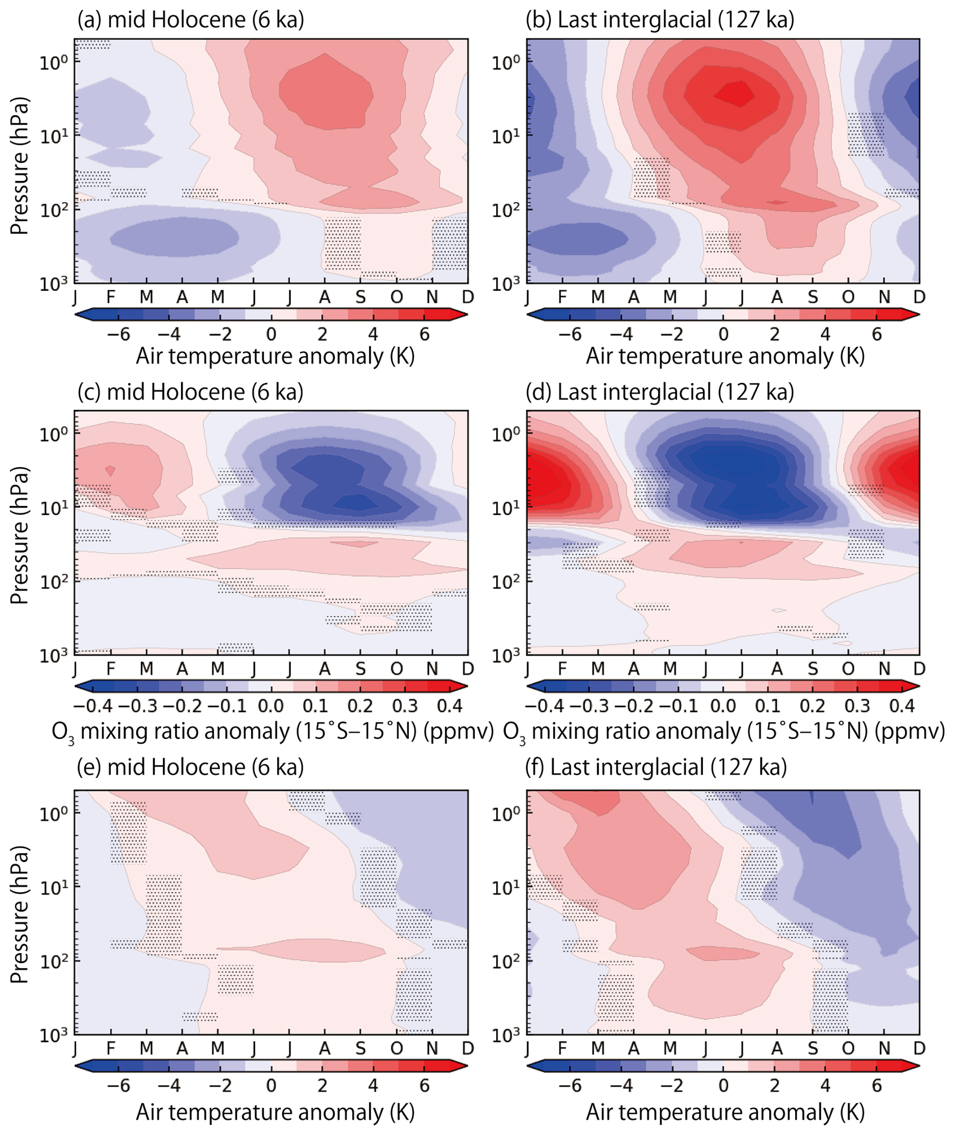
Figure 5 Vertical-seasonal plot of the air temperature anomaly (a, b) and ozone concentration (c, d) at the tropic region (15° S–15° N) relative to the preindustrial condition during the mid-Holocene (MH) (MHcontrol–PIcontrol) (a, c) and the Last Interglacial (LIG) (LIGcontrol–PIcontrol) (b, d). Vertical-seasonal plot of the ozone-induced air temperature anomaly (e, f) at the tropic region (15° S–15° N) relative to the preindustrial condition during the mid-Holocene (MH) (MHcontrol–PIcontrol–MHnoChem + PInoChem) (e) and the Last Interglacial (LIG) (LIGcontrol–PIcontrol–LIGnoChem + PInoChem) (f). The dotted area represents the region where 95 % confidence interval was not achieved.

The ozone-induced changes in air temperature in the MH and LIG are shown in Fig. 5e and f, respectively. In the upper stratosphere, the ozone-induced temperature anomaly is driven by the ozone concentration anomaly through the absorption of short-wave radiation. This signal propagates into the lower stratosphere. For the case of the LIG, the positive ozone anomaly originated from the upper stratosphere between January and May is present in the lower stratosphere between February and August, whose impact is larger than 1 K. This signal may partly propagate into the troposphere, but this tropospheric signal may also be associated with the direct heating due to the increased short-wave radiations into the troposphere. These results indicate that the different astronomical forcing during the MH and LIG affect the air temperature not only in the upper stratosphere, but also in the lower stratosphere and troposphere.

The zonally averaged surface air temperature anomalies in the MH and LIG are shown in Fig. 6. Comparing the air temperature anomalies obtained for the control experiments and those obtained for the noChem experiments, the impact of the atmospheric ozone changes on the zonally averaged climate is small in both the MH and LIG in the south of 60° N. Notably, this contradicts the results shown by Noda et al. (2017), which suggest a warming in the Southern Hemisphere in the MH. The largest influence of stratospheric ozone on the zonal annual mean surface air temperature is observed in the north of 60° N. In both the MH and LIG, our results show a cooling of the zonally averaged temperature at the high-latitude regions of the Northern Hemisphere, which was not seen in the results shown by Noda et al. (2017). Near the North Pole, the ozone-induced change in the zonal annual mean surface air temperature is ∼ 0.35 and 0.25 K in the MH and LIG, respectively.

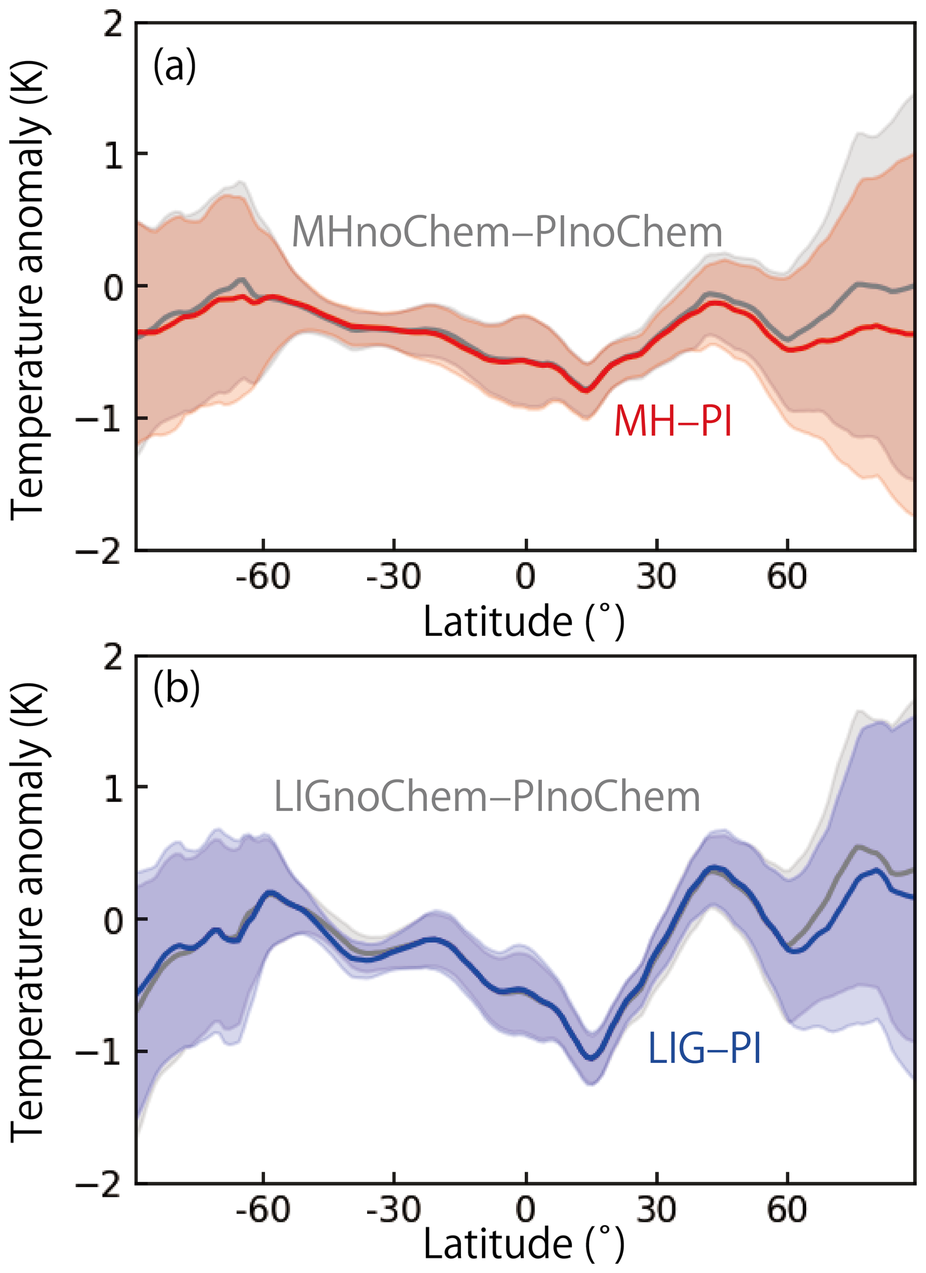
Figure 6 Zonally averaged annual mean temperature anomaly for (a) mid-Holocene (MH) and (b) Last Interglacial (LIG) conditions compared with the preindustrial (PI) condition. The red and blue lines represent the zonally mean surface air temperature anomaly for the MH and LIG experiments, respectively (MHcontrol–PIcontrol and LIGcontrol–PIcontrol, respectively). The grey lines represent the zonally mean surface air temperature anomaly for the MH and LIG experiments estimated using an atmospheric ozone distribution in PI, respectively (MHnoChem–PInoChem and LIGnoChem–PInoChem, respectively). The hatched regions represent the intervals of 1σ.

3.2 Stratospheric ozone around the South Pole and its impact on climate

We focus on the polar regions around Antarctica, where changes in stratospheric ozone potentially affect wind patterns and hence surface climate (Noda et al., 2017). The air temperature and ozone anomalies in the MH and LIG are shown in Fig. 7a–d. As a result of the smaller insolation, the ozone concentrations in the upper stratosphere around the southern polar region (90–60° S) in the MH and LIG conditions are both higher than that in the PI conditions during the austral summer because the air temperature is lower than in the PI conditions owing to the weaker insolation (Fig. 7c and d). As a result, the ozone concentrations in the upper stratosphere are more than 0.1 ppm higher than the PI conditions during February and March for the MH conditions (Fig. 7c), which is slightly smaller than the peak value estimated in the previous study (Noda et al., 2017). In the LIG conditions, the increase in ozone concentration in the upper stratosphere starts during October and continues until April. This is because the insolation anomaly became negative during October, which results in the earlier onset of the positive anomaly of the ozone concentration compared with the case of the MH conditions (Fig. 3). The positive anomaly of the ozone concentration in the upper stratosphere during the LIG is much stronger than in the MH case, exceeding ∼ 0.3 ppm during January (Fig. 7d).

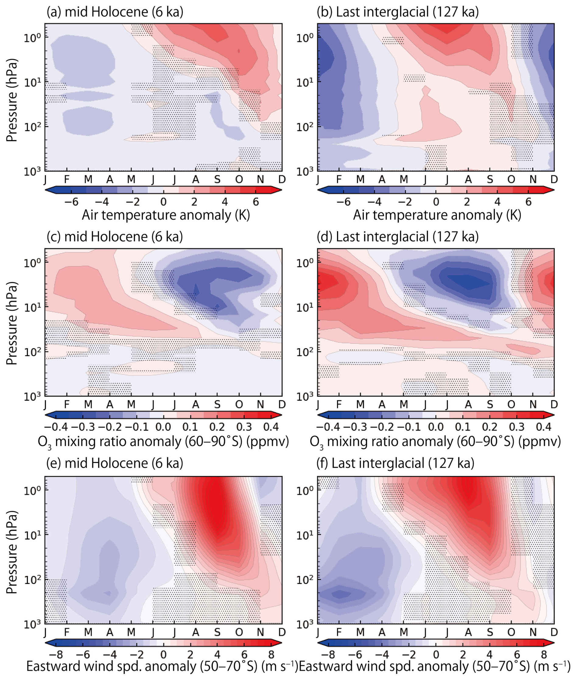
Figure 7 Vertical-seasonal plot of the air temperature anomaly (a, b) and ozone concentration (c, d) at high latitude regions of the southern hemisphere (60–90° S) and eastward wind speed anomaly at mid-latitude regions of the southern hemisphere (50–70° S) (e, f) relative to the preindustrial condition during the mid-Holocene (MH) (MHcontrol–PIcontrol) (a, c, e) and the Last Interglacial (LIG) (LIGcontrol–PIcontrol) (b, d, f). The dotted area represents the region where 95 % confidence interval was not achieved.

The positive ozone anomaly in the upper stratosphere during the austral summer is transported into the lower stratosphere during the austral autumn and winter, where the ozone lifetime is relatively long owing to the polar night (Noda et al., 2017). As a result, the positive ozone anomaly persists in the lower stratosphere (∼ 100 hPa) until March of the following year for the MH case (Fig. 7c). For the LIG case, the positive anomaly is stronger than in the MH, and it persists in the lower stratosphere throughout the year (Fig. 7d). In this case, the positive anomaly was over 0.05 ppm throughout the year. This may have contributed to warming the lower stratosphere, especially from February to June, as indicated by the contribution to air temperature from ozone changes (Fig. 8b).

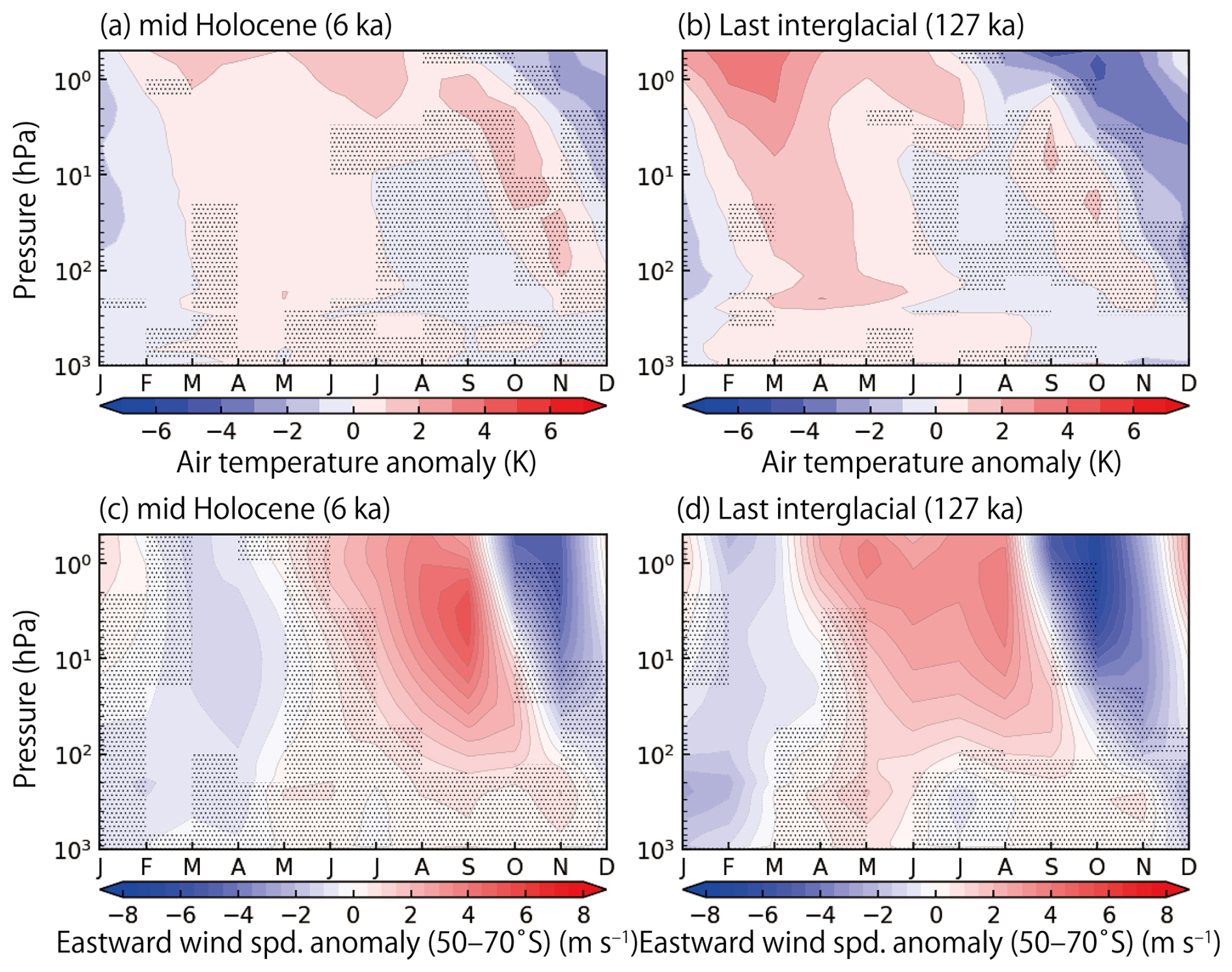
Figure 8 Vertical-seasonal plot of the ozone-induced air temperature anomaly (a, b) and ozone-induced eastward wind speed anomaly at mid-latitude regions of the southern hemisphere (50–70°) (c, d) relative to the preindustrial condition during the mid-Holocene (MH) (MHcontrol–PIcontrol–MHnoChem + PInoChem) (a, c) and the Last Interglacial (LIG) (LIGcontrol–PIcontrol–LIGnoChem + PInoChem) (b, d). The dotted area represents the region where 95 % confidence interval was not achieved.

During the austral winter to spring, the ozone concentration anomaly in the upper stratosphere decreases owing to the high air temperature (Fig. 7a–d). The negative anomaly drops down to ∼ 0.2 and ∼ 0.3 ppm for the case of the MH and LIG, respectively. Concurrently, the strength of the southern westerly jet increases dramatically during the austral winter and spring (Fig. 7e and f). The wind speed increases to more than 8 m s⁻¹ during both the MH and LIG. This intensification of the southern westerly jet works opposite to the effect from changes in the ozone distribution inferred from the previous study (Noda et al., 2017). The westerly jet intensity is related to the meridional air temperature gradient in the stratosphere at the mid-latitude regions. In the southern hemisphere, the meridional temperature anomaly is large owing to the different insolation forcing in the austral winter in the MH and LIG (Figs. 3c–d, 5a–b, and 7a–b). Notably, the intensification of the westerly jet is accelerated by the change in the atmospheric ozone in both the MH and LIG (Fig. 8c and d), even though the ozone-related positive air temperature anomaly does not indicate a larger meridional temperature gradient during the austral winter and spring (Figs. 5e–f and 8a–b).

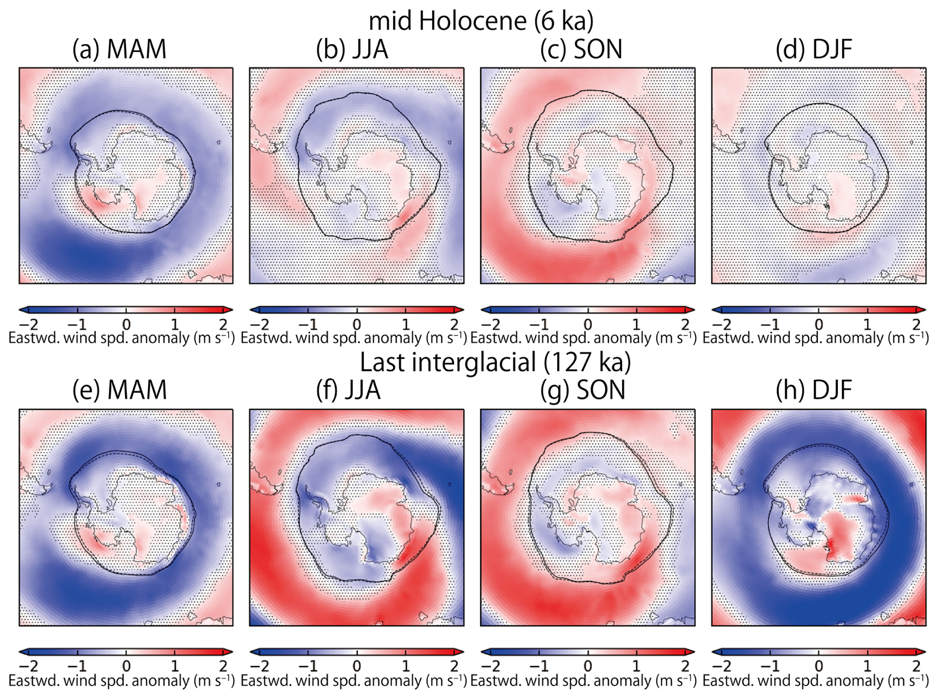
Figure 9 Eastward near-surface (10 m) wind anomaly around the South Pole relative to the preindustrial condition for MAM, JJA, SON, and DJF during the mid-Holocene (MH) (MHcontrol–PIcontrol) (a–d) and the Last Interglacial (LIG) (LIGcontrol–PIcontrol) (e–h). The dotted area represents the region where 95 % confidence interval was not achieved. The dashed line represents the boundary of the sea ice concentration of 15 % for the PIcontrol experiment. The solid line represents that for MHcontrol (a–d) and LIGcontrol (e–h) experiments, respectively.

The positive wind anomaly in the stratosphere during the austral winter propagates into the troposphere in the austral spring (Fig. 7e, and f). The seasonal changes in the near-surface wind speed (10 m) anomaly are shown in Fig. 9. During SON, the near-surface wind speed increases over a wide area of the ∼ 40–60° S region in both the MH and LIG (Fig. 9b, c, f, and g). During DJF and MAM, the near-surface wind speed decreases compared with the PI conditions over a wide area of the ∼ 50–60° S region in the LIG (Fig. 9a, b, e, and f). This wind response would be caused primarily by the decrease of the meridional temperature gradient in the troposphere because of the cooling of the troposphere in the tropics in DJF and MAM (Fig. 5a and b), which is stronger than that in the high-latitude region (Fig. 7a and b). The response of the surface air temperature is asymmetric zonally in JJA and SON during the LIG (Fig. 10f and g). In addition, the ozone-related change in the surface air temperature summarised in Fig. 11 exhibits the asymmetric effect in JJA and SON, especially in the LIG, while regions with significant signals are limited (Fig. 11f and g). These results indicate that the change in the atmospheric ozone affects the surface air temperature only regionally.

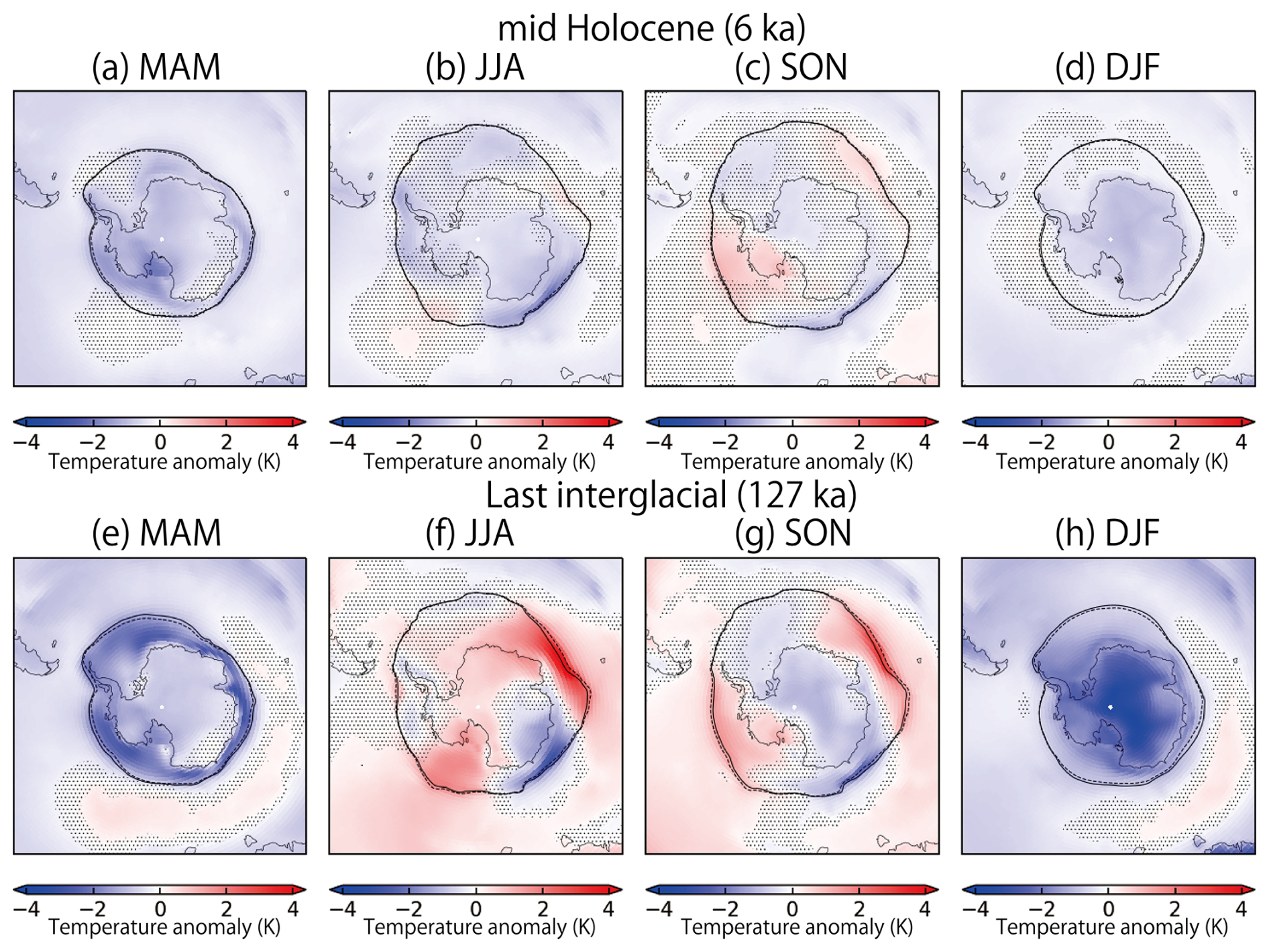
Figure 10 Surface air temperature anomaly around the South Pole relative to the preindustrial condition for MAM, JJA, SON, and DJF during the mid-Holocene (MH) (MHcontrol–PIcontrol) (a–d) and the Last Interglacial (LIG) (LIGcontrol–PIcontrol) (e–h). The dotted area represents the region where 95 % confidence interval was not achieved. The dashed line represents the boundary of the sea ice concentration of 15 % for the PIcontrol experiment. The solid line represents that for MHcontrol (a–d) and LIGcontrol (e–h) experiments, respectively.

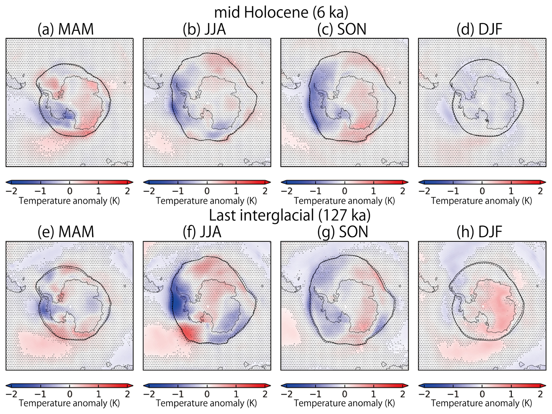
Figure 11 Ozone-induced surface air temperature anomaly around the South Pole relative to the preindustrial condition for MAM, JJA, SON, and DFJ during the mid-Holocene (MH) (MHcontrol–PIcontrol–MHnoChem + PInoChem) (a–d) and the Last Interglacial (LIG) (LIGcontrol–PIcontrol–LIGnoChem + PInoChem) (e–h). The dotted area represents the region where 95 % confidence interval was not achieved. The dashed line represents the boundary of the sea ice concentration of 15 % for the PIcontrol experiment. The solid line represents that for MHcontrol (a–d) and LIGcontrol (e–h) experiments, respectively.

3.3 Stratospheric ozone around the North Pole and its impact on climate

The changes in stratospheric ozone would decrease the surface air temperature in the high-latitude regions of the northern hemisphere in both MH and LIG (Fig. 6). The responses of the air temperature and ozone anomalies at 60–90° N are summarized in Fig. 12. The notable difference in the vertical structure of air temperature anomaly around the North Pole compared with the case around the South Pole is that the negative temperature anomaly from November to March does not propagate strongly into the lower stratosphere (Fig. 12a and b). This would reflect the small insolation due to the polar night in the winter in the northern hemisphere. Instead, the positive anomaly in summer propagated strongly into the lower stratosphere compared with the case of the regions around the South Pole, reflecting the stronger insolation in the northern hemisphere. It is also notable that the air temperature in summer and autumn around the North Pole is high in the troposphere in both MH and LIG, which may reflect the warming of the surface due to insolation forcing (Fig. 12a and b).

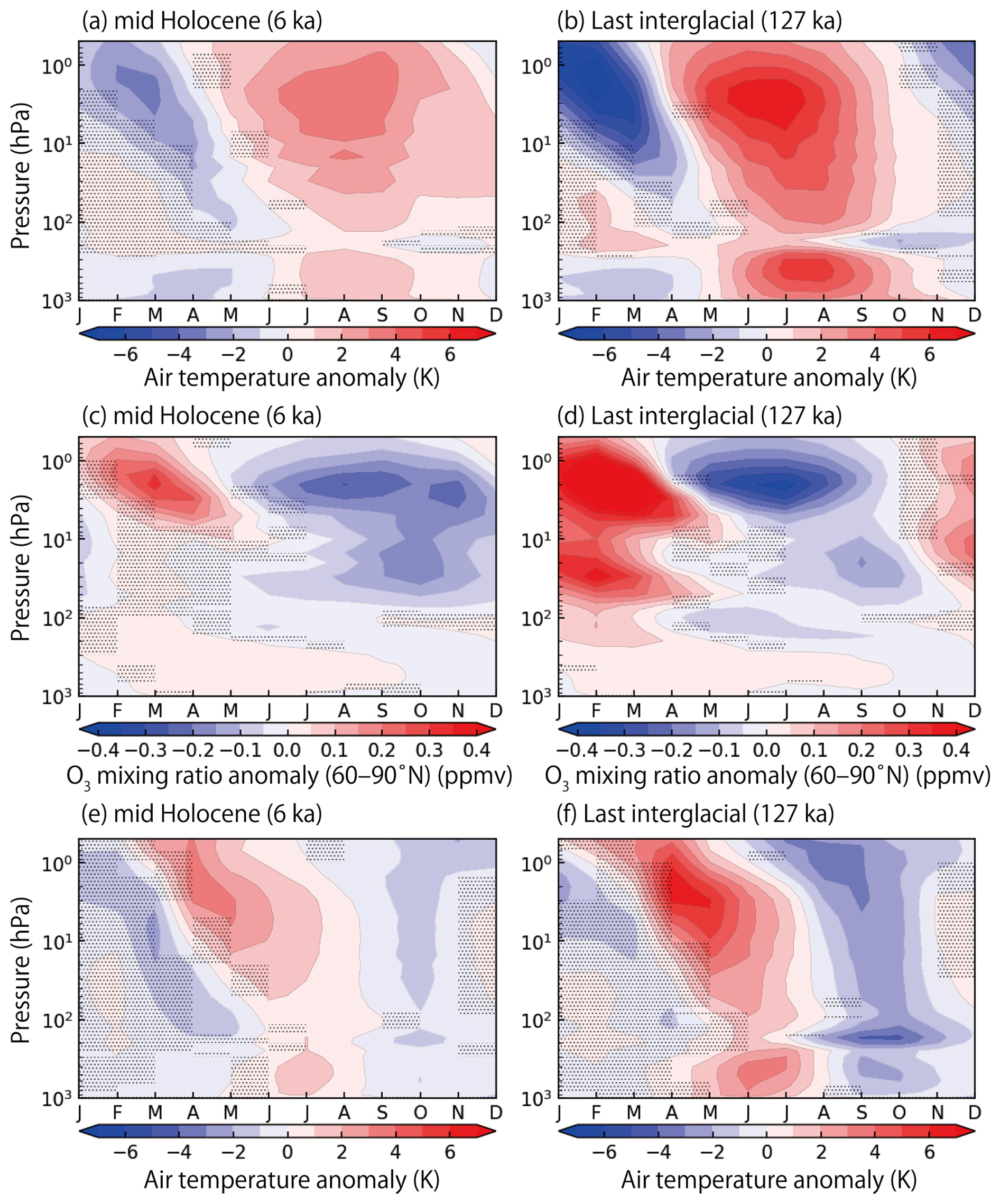
Figure 12 Vertical-seasonal plot of the air temperature anomaly (a, b) and ozone concentration (c, d) at the high-latitude regions of the northern hemisphere (60–90° N) relative to the preindustrial condition during the mid-Holocene (MH) (MHcontrol–PIcontrol) (a, c) and the Last Interglacial (LIG) (LIGcontrol–PIcontrol) (b, d). Vertical-seasonal plot of the ozone-induced air temperature anomaly (e, f) at the high-latitude regions of the northern hemisphere (60–90° N) relative to the preindustrial condition during the mid-Holocene (MH) (MHcontrol–PIcontrol–MHnoChem + PInoChem) (e) and the Last Interglacial (LIG) (LIGcontrol–PIcontrol–LIGnoChem + PInoChem) (f). The dotted area represents the region where 95 % confidence interval was not achieved.

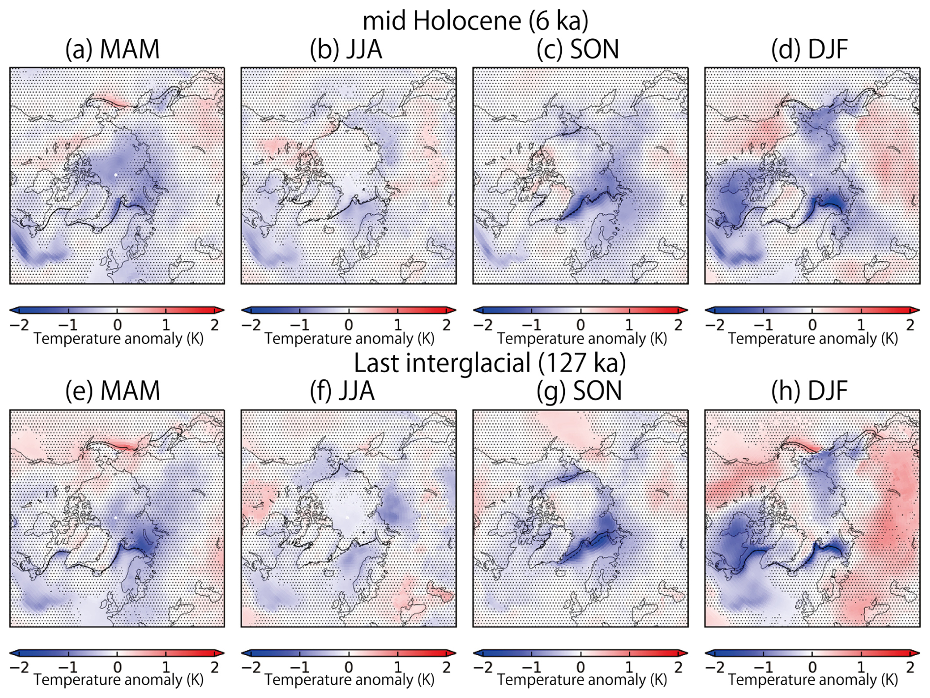
Figure 13 Ozone-induced surface air temperature anomaly around the North Pole relative to the preindustrial condition for MAM, JJA, SON, and DJF during the mid-Holocene (MH) (MHcontrol–PIcontrol–MHnoChem + PInoChem) (a–d) and the Last Interglacial (LIG) (LIGcontrol–PIcontrol–LIGnoChem + PInoChem) (e–h). The dotted area represents the region where 95 % confidence interval was not achieved. The dashed line represents the boundary of the sea ice concentration of 15 % for the PIcontrol experiment. The solid line represents that for MHcontrol (a–d) and LIGcontrol (e–h) experiments, respectively.

The ozone-induced air temperature anomaly is shown in Fig. 12e and f. The positive temperature anomaly caused by the increase of ozone from February to May in the upper stratosphere propagates into the lower stratosphere from May to August in both the MH and LIG. The ozone-induced positive temperature anomaly is also found in the troposphere in summer in both MH and LIG, but this tropospheric signal may reflect the increased downward short-wave radiation and associated feedbacks reflecting the changes in stratospheric ozone. The negative temperature anomaly caused by ozone depletion in the upper stratosphere in summer and autumn propagates into the lower stratosphere in both MH and LIG. In this season, the negative ozone anomaly was also seen in the troposphere. The distribution of the ozone-induced surface temperature anomaly is shown in Fig. 13. The cooling is enhanced in the SON and DJF at the edge of the sea ice (Fig. 13c, d, g, and h). While the Arctic sea-ice distributions in the MH and LIG are smaller than in the PI in SON owing to the effect of the different astronomical forcing (black solid lines in Fig. 13), the cooling effect from the changes in ozone distributions suppresses the sea-ice retreat. This ozone-induced net expansion of sea ice would be associated with the intensified eastward wind speed at the edge of the sea ice. This cooling signal, owing to atmospheric ozone, can be seen in all seasons in both MH and LIG (Fig. 13). In summary, these results suggest that changes in stratospheric ozone may affect the surface climate at least regionally around the poles.

4 Discussion

In this study, we investigated the ozone distribution and its impact on atmosphere and climate during the MH and LIG using MRI-ESM2.0. We showed that the ozone anomalies in the upper stratosphere in the MH and LIG exhibit a seasonal cycle reflecting the changes in the astronomical forcing. These signals also affect the ozone distribution in the lower stratosphere via transport and radiation changes. We further showed that the changes in ozone distributions in the MH and LIG decreases the surface air temperature in the high latitude region of the northern hemisphere, reflecting the changes in the sea-ice distribution. In the high latitude region of the southern hemisphere, on the other hand, our result showed that the impact of the changes in stratospheric ozone was seen only seasonally and its impact on the zonal and annual mean averaged surface air temperature in the southern hemisphere was very small. This contrasts with the results presented by Noda et al. (2017), which indicated the ozone-induced increases of surface air temperature over the southern hemisphere in the MH, even though the very similar response of stratospheric ozone distribution. This different response would be attributed to the different response of the westerly jet between our results and Noda et al. (2017). In the previous study, it was pointed out that the changes in the stratospheric ozone distribution would weaken the westerly jet during the austral winter in the MH (Noda et al., 2017). On the other hand, our results showed that the southern westerly jet would strengthen during the austral winter and autumn during the MH and LIG owing to the different astronomical forcing. This different response around Antarctica may be related to the different biases in temperature. For example, the surface air temperature around Antarctica simulated by MRI-ESM2.0 employed in this study exhibits a cool bias, while that simulated by MRI-CGCM3, which is an atmospheric general circulation model used in MRI-ESM1 employed by Noda et al. (2017), exhibits a warm bias, especially over the Southern Ocean (Yukimoto et al., 2019). As a result, the responses of the sea ice distribution and the surface air temperature differed from those reported by Noda et al. (2017). In Noda et al. (2017), the changes in near-surface wind speed are considered to have affected the climate via changing the surface Ekman transport (Noda et al., 2017), which may further modify the sea ice distribution and surface air temperature. On the other hand, the result of this study exhibits zonally asymmetric characteristics and the ozone-induced near-surface wind and sea ice distribution changes inferred in Noda et al. (2017) do not occur in our results. In MRI-ESM2.0, the sea-ice extent around Antarctica is slightly higher than observations and MRI-CGCM3, but it reproduces the sea-ice edge around Antarctica well (Yukimoto et al., 2019). The reproduction of sea ice extent in the Arctic Ocean in MRI-ESM2.0 was much closer to the observations than that of MRI-CGCM3. These different sea-ice distributions may have also contributed to the different responses between the models. Specifically, for the case of the LIG, the sea ice may have completely melted seasonally (Guarino et al., 2020; Diamond et al., 2021; Sime et al., 2023). In this case, the ozone-induced climatic impact of the changes in sea-ice distributions in the Arctic Ocean may have been smaller than in our model. For further quantitative constraints on the role of the stratospheric ozone in paleoclimates, it should be investigated using multiple Earth system models with interactive ozone.

While the reconstruction of stratospheric ozone in the past is not available, the tropospheric ozone burden during the LIG was estimated based on a record of the clumped isotope composition of O₂ in the East Antarctic ice core (Yan et al., 2022), indicating a reduction in the tropospheric ozone burden by nearly 9 % compared with the PI conditions. It has been inferred that the dispersal of modern humans had not yet occurred during the LIG (Liu et al., 2015; Malaspinas et al., 2016; Groucutt et al., 2018), which makes the LIG an ideal period for reconstructing the tropospheric ozone under a smaller impact from the influence of humans (Yan et al., 2022). However, the tropospheric ozone concentration may be affected not only by factors such as astronomical forcing, but the activity of early humans. For example, early humans could affect the supply rate of methane to the troposphere through rice cultivation. Indeed, ice core records indicate that the atmospheric methane level has increased since the MH compared with the LIG (Spahni et al., 2005; Singarayer et al., 2011), which would be associated with rice cultivation (Ruddiman, 2003; Ruddiman et al., 2008) and/or natural wetland emissions (Schmidt and Shindell, 2004; Sowers, 2010; Singarayer et al., 2011). The early human activity can affect the supply rate of NO_x to the troposphere by causing wildfire events (Ward et al., 2012). The magnitude of wildfire events is determined by the complex interrelationship between climate, vegetation activities, and early human activities, so it would also be affected by the different astronomical forcing. Because our model does not consider the different source fluxes of these gases, the simulated tropospheric ozone should not be compared with the reconstructions. Simulations of the last glacial cycle using a fully coupled Earth system model including the atmosphere, ocean, aerosol, ozone chemistry, and vegetation cycle would be ideal for understanding the variations in the tropospheric ozone distribution during this period.

5 Conclusions

This study investigates the climate and atmospheric ozone simulated by MRI-ESM2.0. The response of the atmospheric ozone during the MH is similar to the results of the previous study. The pattern of the atmospheric ozone response during the LIG is similar to that during the MH, but the intensity of the variation is stronger than in the MH. The southern westerly jet intensifies compared with the PI conditions during the austral winter and spring owing to the effect from the astronomical forcing, which is further amplified by the variations in the atmospheric ozone. The change in the atmospheric ozone decreases the surface air temperature in the high-latitude regions of the northern hemisphere by ∼ 0.3 K, while it affects the surface air temperature around Antarctica only regionally and seasonally during the MH and LIG.

Appendix A: Climate in the mid-Holocene and Last Interglacial

In this Appendix, we summarize the simulated climate state in the MH and LIG. The 150-year mean value of the surface (2 m) air temperature and total precipitation rate during the MH and LIG are shown in Fig. A1. The global annual mean surface air temperatures were ∼ 13.7 and ∼ 13.8 °C under the MH and LIG conditions, respectively, and both were lower than that of our PI-control experiment (∼ 14.1 °C). Although the paleoclimate proxy indicates a warmer environment during the MH and LIG, the model does not simulate the higher global annual mean surface air temperature, which is similar to the results from other climate models (Liu et al., 2014; Brierley et al., 2020). The decrease in the global annual mean surface air temperature is attributed primarily to the decrease in the temperature in North Africa and India owing to the northern shift of the Afro–Asian monsoon system caused by the different sets of orbital parameters, as seen in many climate models (Brierley et al., 2020; Otto-Bliesner et al., 2021). This is also reflected in the increased total precipitation in these regions in both the MH and LIG (Fig. A1b and d).

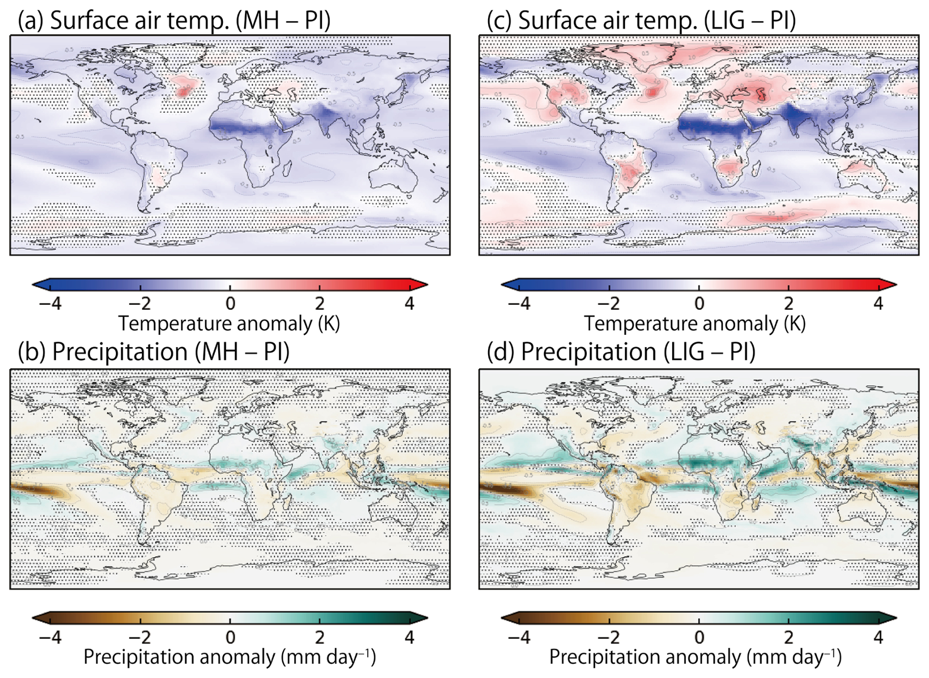
Figure A1 Surface (2 m) air temperature anomaly (a, c) and total precipitation anomaly (b, d) for the mid-Holocene (MH) (MHcontrol–PIcontrol) (a, b) and Last Interglacial (LIG) (LIGcontrol–PIcontrol) (c, d) conditions relative to the preindustrial (PI) condition. The dotted area represents the region where 95 % confidence interval was not achieved.

For the MH case, the enhanced warming over high latitude regions of the northern hemisphere compared with the PI conditions inferred from the paleoclimate proxy was also not simulated (Fig. A1a). Significant warming is observed (∼ 2 K) only over the mid-latitude regions of the Atlantic Ocean. The warming over the Atlantic Ocean compared with the PI conditions is seen in every season (left panels in Fig. A2). Over the North American and Eurasian continents, the global annual mean surface air temperature decreased slightly (Fig. A1a). In these regions, the seasonal cycle of the surface air temperature strengthened compared with the PI conditions (left panels in Fig. A2). In the JJA (June–August) and SON (September–November) seasons, the surface air temperature in some part of these regions increased by more than 1 K compared with the PI conditions, while it decreased by more than 1 K during the DJF (December–February) and MAM (March–May) seasons. The sea ice concentration around the Arctic Ocean decreased during SON compared with the PI conditions (Fig. A3), reflecting the change in insolation during the MH (Fig. 3a). As a result, the surface air temperature increases by ∼ 1 K over the Arctic Ocean in SON (Fig. A4c), owing to the decreased sea ice concentration (Fig. A3c). During the DJF and MAM, the sea ice extent increased at the Sea of Okhotsk and Bering Sea, reflecting the negative insolation anomaly, which would also affect the surface air temperature.

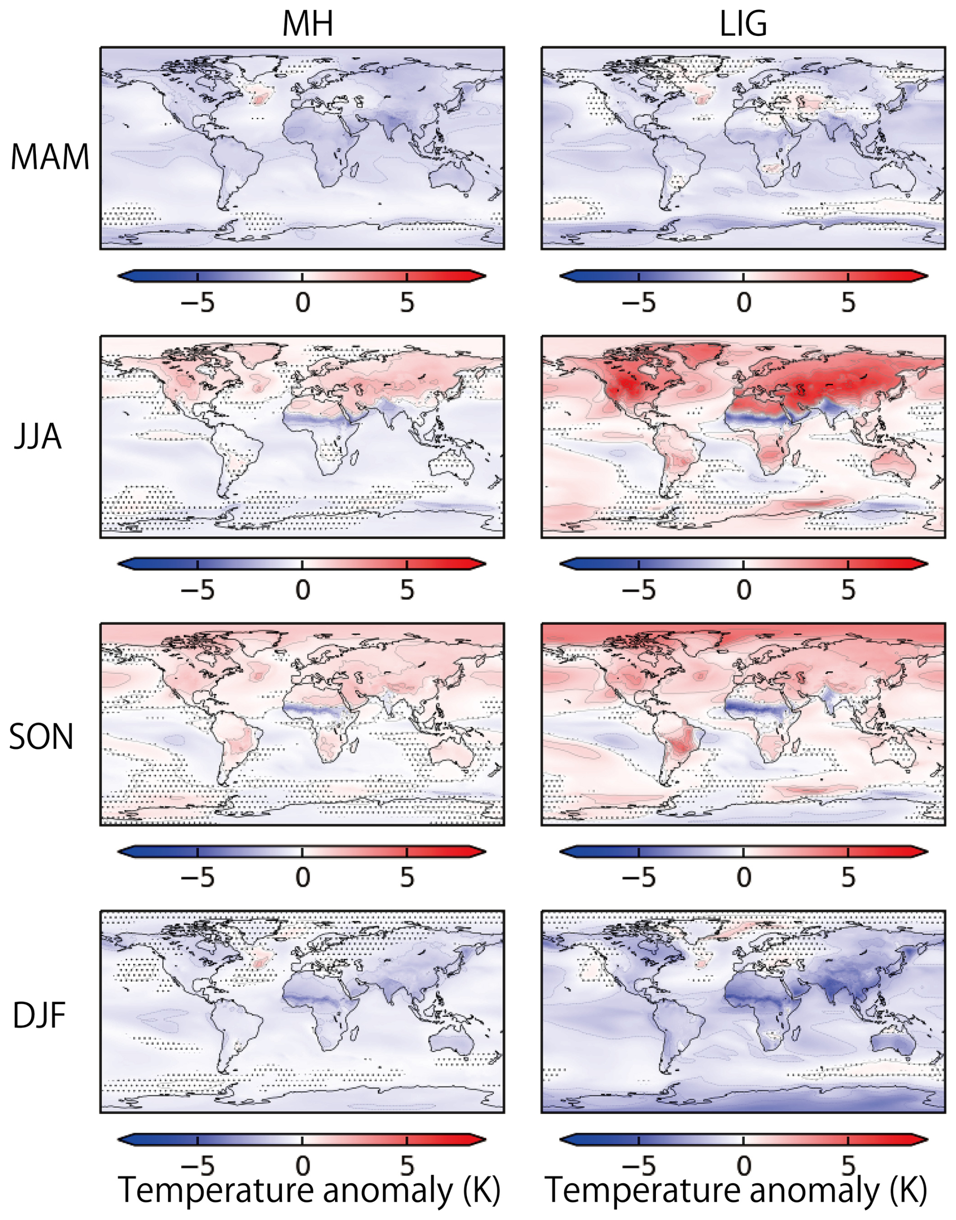
Figure A2 Surface air temperature anomaly relative to the preindustrial condition for MAM, JJA, SON, and DJF during the mid-Holocene (MH) (MHcontrol–PIcontrol) (left panels) and the Last Interglacial (LIG) (LIGcontrol–PIcontrol) (right panels). The dotted area represents the region where 95 % confidence interval was not achieved.

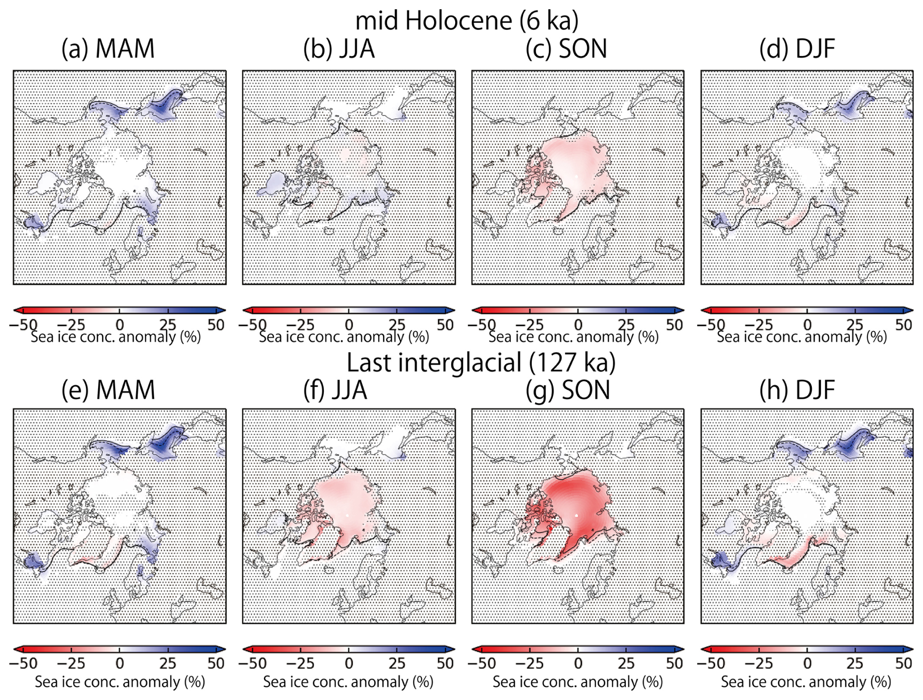
Figure A3 Sea ice concentration anomaly around the Arctic Ocean relative to the preindustrial condition for MAM, JJA, SON, and DJF during (a–d) the mid-Holocene (MH) (MHcontrol–PIcontrol) and (e–h) the Last Interglacial (LIG) (LIGcontrol–PIcontrol). The dotted area represents the region where 95 % confidence interval was not achieved. The dashed line represents the boundary of the sea ice concentration of 15 % for the PIcontrol experiment. The solid line represents that for MHcontrol (a–d) and LIGcontrol (e–h) experiments, respectively.

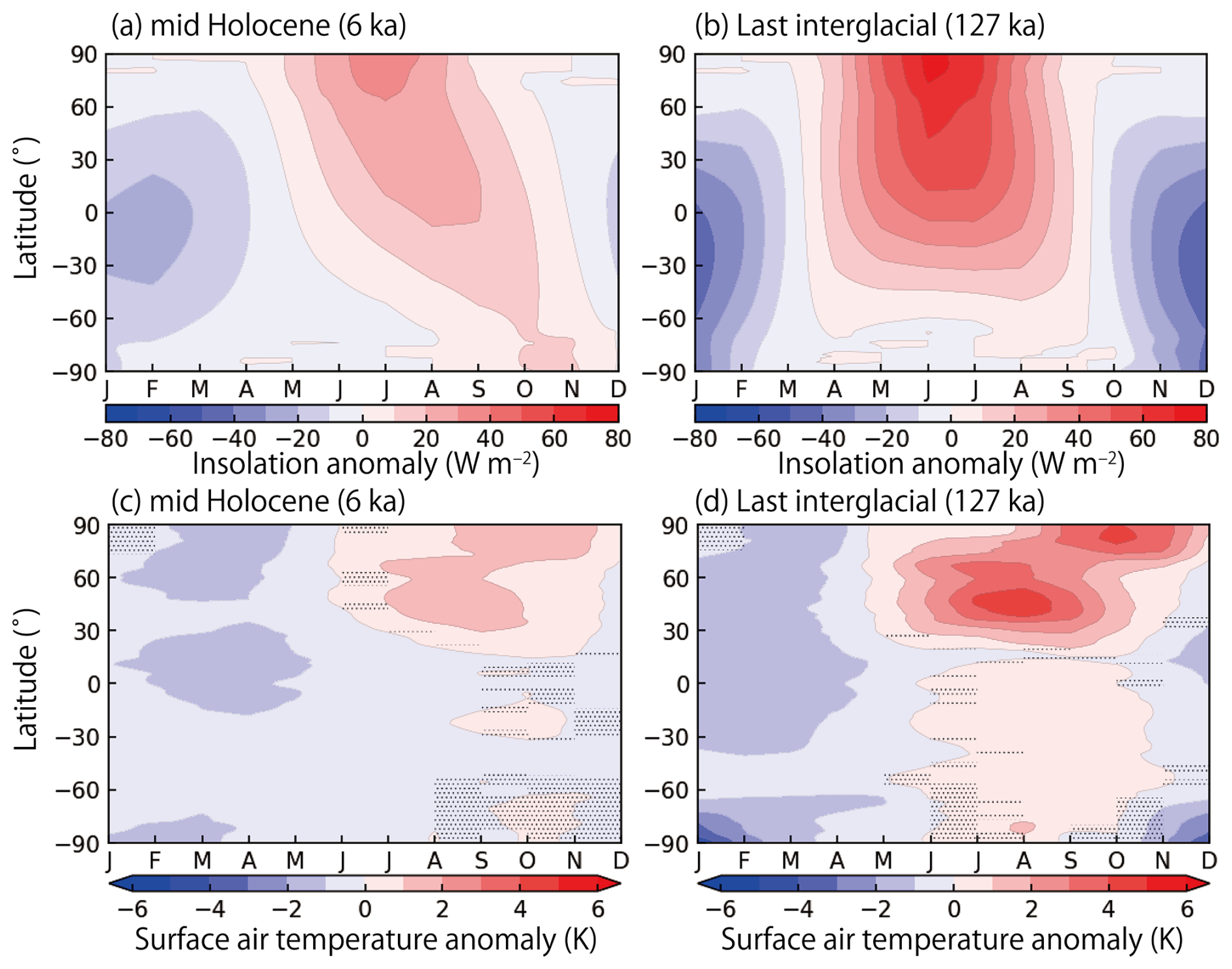
Figure A4 Top-of-atmosphere insolation anomaly and surface (2 m) air temperature anomaly for the mid-Holocene (MH) condition (a and c, respectively) (MHcontrol–PIcontrol) and the Last Interglacial condition (b and d, respectively) (LIGcontrol–PIcontrol), relative to the preindustrial condition. The dotted areas in panels (c) and (d) represent the region where 95 % confidence interval was not achieved.

For the LIG case, the overall patterns of the surface air temperature anomaly from the PI conditions were similar to the MH, but the signal tended to be stronger, which was similar to the previous study (Otto-Bliesner et al., 2021). The sea ice concentration during SON decreased over a wide area of the Arctic Ocean (Fig. A3g). The ice edge retreated compared with the PI in the Greenland Sea and Barents Sea. However, it did not exhibit the complete loss of sea ice simulated by previous studies (Guarino et al., 2020; Diamond et al., 2021; Sime et al., 2023) as in many other climate models (Kageyama et al., 2021). Nevertheless, significant warming was observed in JJA and SON (right panels in Fig. A2), reflecting the higher insolation anomaly and the associated response of sea ice distribution (Figs. 3b and A3). In SON, specifically, the surface air temperature over the Arctic Ocean increases by more than ∼ 4 K compared with the PI conditions (Fig. A4d). As a result, significant warming is observed in the annual mean temperature over the regions covering the Greenland Sea, Norwegian Sea, and Barents Sea (Fig. A1c). The warming is also observed in the central part of North America, the southern part of South America and Africa, the northern part of Australia, the western part of the Eurasian continent, and in part of the Southern Ocean. Despite the warming in these regions, the global annual mean surface air temperature did not exceed the PI value.

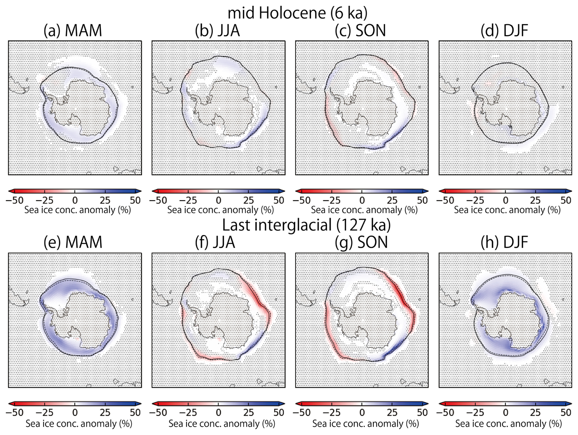
Figure A5 Sea ice concentration anomaly around the South Pole relative to the preindustrial condition for MAM, JJA, SON, and DJF during the mid-Holocene (MH) (MHcontrol–PIcontrol) (a–d) and the Last Interglacial (LIG) (LIGcontrol–PIcontrol) (e–h). The dotted area represents the region where 95 % confidence interval was not achieved. The dashed line represents the boundary of the sea ice concentration of 15 % for the PIcontrol experiment. The solid line represents that for MHcontrol (upper panels) and LIGcontrol (lower panels) experiments, respectively.

The surface air temperature and sea ice distributions in the high-latitude regions of the Southern Hemisphere during the MH and LIG are shown in Figs. 10 and A5, respectively. During the MH and LIG, the sea ice concentration anomaly in the Southern Ocean relative to the PI conditions exhibits a zonally asymmetric pattern in JJA and SON, associated with the surface air temperature anomaly (Figs. 10 and A5). The simulated patterns in JJA and SON were similar to the distribution anomaly owing to the direct influence of insolation simulated in the previous study (Pedersen et al., 2017). On the other hand, during the MH, the patterns of the sea ice concentration anomaly relative to PI in JJA differed from that in the previous study (Noda et al., 2017), which estimated that the sea ice concentration would increase in JJA in this region. In DJF and MAM, the sea ice concentration increased significantly in the case of the LIG. During the MH, the sea ice concentration showed a very small change in DJF, most of which was not significant (Fig. A5d). In MAM, the sea ice concentration increased significantly during the MH compared with the PI conditions (Fig. A5a).

For both the MH and LIG, our model did not simulate higher global and annual mean surface air temperature than that in the PI period, which is similar to the situations of many other climate models simulating the MH (Liu et al., 2014; Brierley et al., 2020) and the LIG (Lunt et al., 2013; Masson-Delmotte et al., 2013; Otto-Bliesner et al., 2013, 2020; Williams et al., 2020; Otto-Bliesner et al., 2021; Zhang et al., 2021). The colder temperature is attributed primarily to the cold temperature in the Sahara and Sahel regions in North Africa, as observed in many other models (Lunt et al., 2013; Brierley et al., 2020; Otto-Bliesner et al., 2021), which would be associated with the formation of clouds in these regions. It has been discussed from the paleoclimate records that much of the present Sahara Desert was covered by grassland during the MH and LIG (Hoelzmann et al., 1998; Bartlein et al., 2011; Tarasov et al., 2013; Hély et al., 2014; Hoogakker et al., 2016; Harrison, 2017; Phelps et al., 2020). This would be associated with the bistable characteristics of the vegetation cover in this region and an abrupt transition to a vegetated state (Brovkin et al., 1998; Hopcroft and Valdes, 2021, 2022). A study using a climate model inferred that this may contribute to a warmer global annual mean surface temperature during the MH (Thompson et al., 2022). In addition, a simulation with decreased dust emission from the Sahara Desert assuming the greening of Sahara indicates that the reduced dust emission may help warm the surface (Liu et al., 2018). These results indicate that a reproduction of the greening of the Sahara Desert would be key for achieving a warm climate during the MH and LIG in climate models. Recently, some studies have reproduced the greening of the Sahara Desert using climate models coupled with a dynamic vegetation model (Lu et al., 2018; Hopcroft and Valdes, 2021; Hopcroft et al., 2021; Duque-Villegas et al., 2022; Specht et al., 2024), while many other climate models failed to reconstruct the greening (Joussaume et al., 1999; O'ishi and Abe-Ouchi, 2011; Harrison et al., 2015). To sustain the greening of the Sahara Desert, feedback that helps sustain the precipitation over this region may be necessary, including the formation of large lakes (Contoux et al., 2013; Li et al., 2023). Indeed, a recent model that dynamically simulates the vegetation and lake distributions indicates the greening of the Sahara (Specht et al., 2024). Currently, the land surface type in the atmospheric model of MRI-ESM2.0 has not changed dynamically in accordance with climate changes. Future studies considering these processes in Earth system models would be highly desirable for understanding the dynamics of the greening of the Sahara Desert and the warm climate during the MH and LIG.