Ocean control on sea ice in the Nordic Seas

To better understand the processes in the Nordic Seas and their connection to large-scale climate changes during Dansgaard-Oeschger (D-O) events, we reconstruct sea ice extent (SIE) and subsurface temperatures (SubSTs) in the eastern Fram Strait between 40 and 33.5 ka b2k. Our new proxy data from MD99-2304 reveal pronounced fluctuations in SIE and SubSTs both between and within each investigated Greenland Stadial (GS) and Greenland Interstadials (GIs). Consequently, variations in SIE and SubSTs in the eastern Fram Strait show a weaker connection to climate oscillations in Greenland ice cores, in comparison to changes observed in the southeastern Nordic Seas and the North Atlantic.

Integrating our results with Atlantic Meridional Overturning Circulation (AMOC) strength reconstruction and sea ice records from the southeastern Nordic Seas, we identify different sea ice regimes between the eastern Fram Strait and the southeastern Nordic Seas. These findings suggest that fluctuations in the eastern Fram Strait were primarily driven by shifts in northward oceanic heat transport, which were regulated by changes in the strength of the AMOC.

1 Introduction

A series of rapid climate oscillations known as the Dansgaard–Oeschger (D-O) events characterized Marine Isotope Stage (MIS) 3 (Dansgaard et al., 1982; North Greenland Ice Core Project members, 2004). Each D-O event featured an abrupt warming to a mild Greenland Interstadial (GI) state and then a gradual cooling to a glacial Greenland Stadial (GS) state. These shifts were considered repeated oscillations based on Greenland ice core δ¹⁸O records (Mogensen, 2009; Rasmussen et al., 2014). While the duration and amplitude of changes between each event differ as seen in Greenland δ¹⁸O records, the succession of events and types of signals within the GSs and GIs were comparable (Rasmussen et al., 2014). Several paleoenvironmental reconstructions and modeling studies have suggested that the sea ice extent (SIE) in the Nordic Seas experienced consistent shifts between an extensive sea ice cover during GSs and seasonal sea ice cover during GIs (e.g., Dokken et al., 2013; Hoff et al., 2016; Sadatzki et al., 2019, 2020; Pedro et al., 2022; El bani Altuna et al., 2024a). In the Faroe-Shetland Channel, SIE reductions consistently occurred before Greenland warming, while its expansion preceded Greenland cooling. These on/off SIE signals were observed consistently for all D-O events between 30 and 40 ka b2k (Sadatzki et al., 2019, 2020). Such shifts in SIE were proposed to have contributed to the D-O climate oscillations through their impact on ocean-ice-atmosphere interactions (Li and Born, 2019; Pedro et al., 2022). In the northernmost Nordic Seas, specifically the Fram Strait, persistent sea ice coverage occurred throughout both GSs and GIs (El bani Altuna et al., 2024a). Based on analyses of a series of idealized model experiments, Buizert et al. (2024) argued that the North Atlantic wintertime sea ice cover was more critical than that in the Nordic Seas for influencing the Greenland ice core D-O signal, due to differences in moisture transport pathways. The Nordic Seas are separated from the North Atlantic by the Greenland-Scotland Ridge, and is a well-established collective term for the Norwegian, Iceland, and Greenland Seas (Fig. 1). These past studies presented a consistent picture of the relationship between Nordic Seas SIE and Greenland climate records, with a steadily repetitive pattern of variability through the course of the D-O events. However, a recent study by Wong et al. (2024) showed that polynyas were present in the eastern Fram Strait through much of HS-4 (also known as GS-9). The presence of polynyas indicated that parts of the northernmost Nordic Seas experienced ice-free conditions, contrasting with previous studies that argued for a perennial sea ice cover north of the Vøring Plateau (Sadatzki et al., 2020; El bani Altuna et al., 2024a). This polynya activity was suggested to be a response to ocean sensible heat flux (Wong et al., 2024). Wong et al. (2024) also showed that the seasonal sea ice cover retreated to the eastern Fram Strait during GI-8, documenting that there were more ice-free areas in the Nordic Seas during GI-8 than formerly proposed (Sadatzki et al., 2019, 2020; El bani Altuna et al., 2024a).

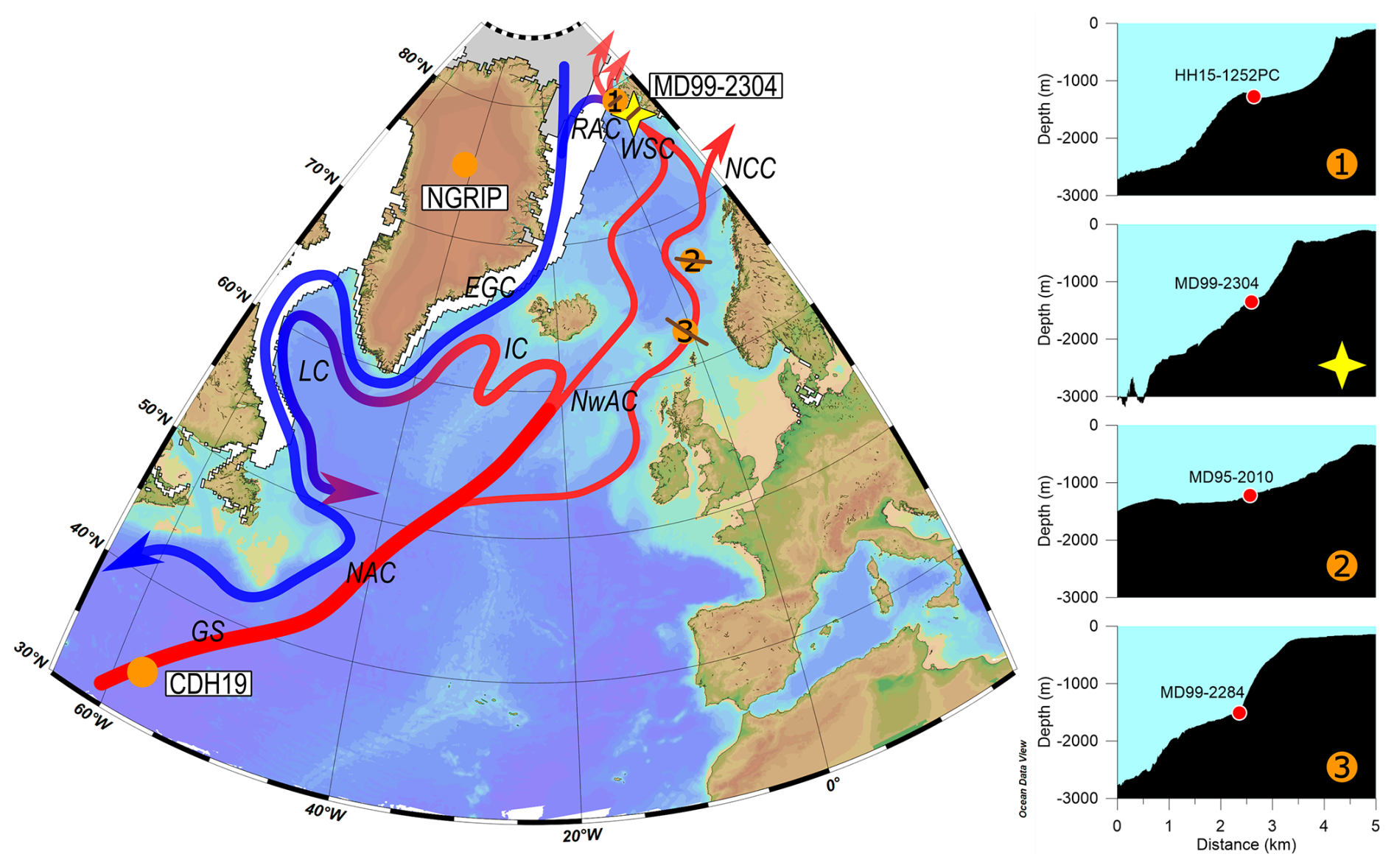
Figure 1 Map of the research area with modern-day conditions (updated from Wong et al., 2024). Core MD99-2304 is highlighted with a light-yellow star. For a comprehensive understanding of SIE across different periods, we compare our results with biomarker data from (1) HH15-1252PC (El bani Altuna et al., 2024a), (2) MD95-2010 (Sadatzki et al., 2020), (3) MD99-2284 (Sadatzki et al., 2018), and Pa $/$ Th record from CDH19 (Henry et al., 2016b). The 2024 September SIE and 2025 March SIE are marked with gray and white areas, respectively (Fetterer et al., 2017, updated to 2025). The Gulf Stream (GS), North Atlantic Current (NAC), Irminger Current (IC), Norwegian Atlantic Current (NwAC), North Cape Current (NCC), and West Spitzbergen Current (WSC) are illustrated with red arrows, while the East Greenland Current (EGC) and Labrador Current (LC) are depicted by blue or red-blue arrows. Between the WSC and EGC, the Return Atlantic Current (RAC) at intermediate water depth is shown as a red-blue line. The right panel displays the cross profile of each site in the eastern Nordic Seas, indicated by brown lines in the map. The basemap was created using Ocean Data View (Schlitzer, Reiner, Ocean Data View, https://odv.awi.de/ (last access: 10 July 2025), 2025), based on the World Ocean Database.

The results from Wong et al. (2024) suggested that sea ice in the northernmost Nordic Seas may have behaved differently during GSs and GIs than previously thought. However, it remains unknown whether polynya activity was a regularly occurring phenomenon in the northernmost Nordic Seas also during other stadials, or if it was limited to HS-4.

Previous studies investigating changes in the Atlantic Meridional Overturning Circulation (AMOC) (Henry et al., 2016a) and Southern Ocean ventilation (Yu et al., 2023) suggested that ocean circulation behavior was not consistent across GSs. This contrasted with the commonly held perspective that climate variability during this period followed a consistently repeating pattern, as observed in Greenland ice core records.

Ocean heat transport and SIE are closely interconnected (e.g., Mahajan et al., 2011; Day et al., 2012; Polyakov et al., 2017; Årthun et al., 2019). Moreover, the heat-laden Atlantic Water (AW) inflow into the Nordic Seas is suggested to be related to the strength of the AMOC (Larson et al., 2020). Therefore, it is reasonable to expect that the varying ocean circulation strength observed during D-O events influenced ocean temperatures as well as SIE in the Nordic Seas. Here we will investigate how the SIE and sea subsurface temperatures (SubSTs) in the Nordic Seas changed through GS-9 to GS-7 (39.9–33.74 ka b2k, thousand years before the year 2000), and whether and how these changes may have been driven by changes in the AMOC.

To do so, we reconstruct the northernmost Nordic Seas SIE semi-quantitively with lipid biomarker proxies and indices, including the highly branched isoprenoids (HBIs) IP₂₅ and HBI-III (Z), sterols brassicasterol and dinosterol, and PIP₂₅ indices from marine sediment core MD99-2304 in the eastern Fram Strait (1348 m water depth; 77°37^′15.6^′′ N 9°56^′54^′′ E) (Fig. 1). We also reconstruct SubSTs based on Mg $/$ Ca measured on planktonic foraminifera from the same sediment core. To evaluate the relationship between ocean circulation and sea ice, we compare our new records from the northernmost Nordic Seas with existing sea ice reconstructions from the eastern Nordic Seas and AMOC reconstruction from the North Atlantic (Henry et al., 2016b). The sea ice records used for comparison are from a site slightly further north in the Fram Strait (core 1 in Fig. 1; El bani Altuna et al., 2024b), the Faroe–Shetland Channel (core 3 in Fig. 1; Sadatzki et al., 2018), and the Vøring Plateau (core 2 in Fig. 1; Sadatzki et al., 2020).

2 Present-day oceanography

The Fram Strait is the northernmost part of the Nordic Seas and one of the main passages where the warm and saline Atlantic Water (AW) enters the Arctic Ocean at intermediate water depths (Smedsrud et al., 2022). The North Atlantic Current (NAC) originates in the Gulf Stream (GS) (Orvik and Niiler, 2002) and travels northward and then eastward across the Atlantic Ocean. It splits into the two-branched Norwegian Atlantic Current (NwAC) and the Irminger Current (IC) (Blindheim and Østerhus, 2005; Bosse et al., 2018). Both branches of the NwAC enter the Nordic Seas over the Greenland-Scotland Ridge. The eastern branch flows along the Norwegian continental slope (Poulain et al., 1996; Bosse et al., 2018). The eastern branch of the NwAC bifurcates in the northern Norwegian Sea, from where the North Cape Current (NCC) flows into the Barents Sea (Ingvaldsen, 2005). The West Spitsbergen Current (WSC), merged with the western branch of the NwAC, flows into the eastern Fram Strait (Furevik, 2001; Bosse et al., 2018) (Fig. 1).

The AW is gradually densified due to ocean heat loss during the northward transport. In the eastern Fram Strait, the densified AW submerges, before entering the Arctic Ocean over the Yermak Plateau or turning southwards, through the Return Atlantic Current (RAC), at intermediate depths (Gordon, 1986; Hattermann et al., 2016). Above the RAC, cold and fresh Polar Water (PW) is transported southwards through the East Greenland Current (EGC) along the Greenland continental margin (Fahrbach et al., 2001). Across the Demark Strait, the EGC interacts with the recirculated IC (Holliday et al., 2007). These currents feed into the boundary current in the Labrador Sea, known as the Labrador Current (LC) (Cuny et al., 2002) (Fig. 1).

This current system, which transports multiple water masses across these Northern Seas, is a crucial component of the AMOC (Bryden, 2021). The poleward AW brings heat and salt to high latitudes. The recirculated, densified AW in the Nordic Seas contributes to the formation of North Atlantic Deep Water (NADW) (Hall and Bryden, 1982; Petit et al., 2021). Variations in this ocean circulation system have a great impact on large-scale climate patterns, including sea ice conditions, ocean heat content distribution, atmospheric temperature, and wind patterns (Liu et al., 2017; Årthun et al., 2019; Lozier et al., 2019). The topographic features of the seabed in the Nordic Seas create constraints for incoming water masses, influencing their properties, distribution, and interactions. On a large scale, these features affect the dynamics of ocean currents, shaping the overall circulation patterns in the region (Blindheim and Østerhus, 2005). In the northern Nordic Seas, the narrowing passage constricts the inflow, triggering internal wave breakup and vertical mixing. This process, in turn, influences the thermal structure as the AW continues its northward journey (e.g., Falk-Petersen et al., 2015; Bensi et al., 2019; Zhang et al., 2022) (Fig. 1).

This research focuses on the eastern Fram Strait, where the interaction between the AW inflow and sea ice conditions plays a critical role in shaping regional and large-scale climate and hydrography.

3 Methodology

We measured sea ice biomarkers and Neogloboquadrina pachyderma Mg $/$ Ca ratios from core MD99-2304 to reconstruct SIE and SubSTs in the eastern Fram Strait. These proxies are described in more detail in Sect. 3.2 and 3.3, respectively.

3.1 Chronological framework

The chronology of MD99-2304 was presented in Wong et al. (2024). The low field magnetic susceptibility (K_lf) of MD99-2304 were tuned to the K_lf of the core MD95-2010 from the Vøring Plateau (core 2 in Fig. 1) (Kissel et al., 1999). Tie points were identified at each abrupt transition in the K_lf records (Wong et al., 2024). Through this tuning, we adopted the age model of MD95-2010, which was previously tied to core MD99-2284 from the Faeroe-Shetland Channel. The chronology of MD99-2284 from the Faeroe-Shetland Channel is considered one of the most robust marine age models for this time interval, as each transition in our investigated time interval is directly tied to the Greenland Ice Core Chronology 2005 (GICC05) (Andersen et al., 2006; Rasmussen et al., 2014; Seierstad et al., 2014) through the identification of identical microtephra layers in the marine core and in Greenland ice cores (Berben et al., 2020; Sadatzki et al., 2020). The age uncertainty is smallest at transitions known to occur within a few decades (Andersen et al., 2006; Rasmussen et al., 2014; Seierstad et al., 2014), and increases further away from these transitions and defined tie points. Jensen et al. (2018) proposed a conservative maximum age mode uncertainty of ca. 500 years for records tuned to the isotope records from the Greenland ice cores. All ages are given as thousand years before the year 2000 (ka b2k).

3.2 Biomarker analysis

Core MD99-2304 was analyzed every 0.5–1 cm (ca. 20–40 years per sample) between 813.25 and 974.75 cm (ca. 40–33.7 ka b2k). Biomarkers were measured in 248 samples. The 149 samples focusing on the HS-4 and GI-8 (ca. 40–36.5 ka b2k, 874.25–974.25 cm) were presented and discussed in Wong et al. (2024). All samples were freeze-dried and homogenized. For biomarker concentration normalization, total organic carbon (TOC) was measured with 90 mg of sediment using a Carbon-Sulfur Analyzer (CS-125, Leco), after the carbonate in sediments was removed with hydrochloric acid (HCl) of 20 % solution.

The internal standards 7-hexylnonadecane (7-HND, 0.066 µg, for IP₂₅ quantification), 9-octylheptadec-8-ene (9-OHD, 0.1 µg, for different quality control procedures), 5α-androstan-3β-ol (androstanol, 10.6 µg, for sterols), and 2,6,10,15,19,23-hexamethyltetracosane (squalane, 3.2 µg, for n-alkanes if needed later) were added to each sample prior to extraction to evaluate instrument stability and analytical accuracy. The total lipid extracts (TLEs) were extracted by ultrasonication for 15 min and centrifugation (2000 rpm) for 3 min, using dichloromethane : methanol (2:1, $v/v$) as a solvent, and the procedure was repeated three times. Then the TLEs were separated using open silica (SiO₂) column chromatography, with n-hexane (5 mL) and ethyl acetate : n-hexane (9 mL, 2:8 $v/v$) as eluent into the hydrocarbon and sterol fractions. The sterol fraction was silylated using 200 µL bis-trimethylsilyl-trifluoroacet-amide (BSTFA) at 60 °C for 2 h. The biomarkers were measured by gas chromatography/mass spectrometry (GC/MS) using an Agilent 7890B GC (30 m DB-1MS column, 0.25 mm i.d., 0.25 µm film thickness) coupled to an Agilent 5977A mass selective detector (MSD, 70 eV constant ionization potential, Scan 50–550 $m/z$, 1 scan s⁻¹, ion source temperature 230 °C, Performance Turbo Pump). Ion monitoring mode (SIM) was selected for HBIs and full scan mode (50–550 $m/z$) for sterols. We focus on two highly branched isoprenoids (HBIs), IP₂₅ and HBI-III (Z), and two sterols, brassicasterol and dinosterol. The selected biomarkers were identified based on their GC retention times in comparison to those of specific reference compounds as well as published mass spectra for HBIs (Belt et al., 2000, 2007) and for sterols (Boon et al., 1979; Volkman, 1986). HBIs were quantified based on their molecular ions, $m/z$ 350 for IP₂₅ and $m/z$ 346 HBI-III (Z), in relation to the fragment ion $m/z$ 266 of 7-HND. Brassicasterol and dinosterol were quantified with molecular ions $m/z$ 470, 500, 472, and 486, respectively, in relation to the molecular ion $m/z$ 348 of androstanol (Wong et al., 2024). An external calibration was applied, to balance different responses of molecular ions of the analytes and the molecular/fragment ions of the internal standards (Fahl and Stein, 2012). To evaluate instrument accuracy and precision, we performed ten replicate measurements of HBIs (e.g., IP₂₅) and sterols on the GC-MSD using a standard sediment. Replicate analyses showed very low variability. For HBIs, 95 % of measurements fell within ±2 standard deviation (SD, σ) of the mean, and for sterols, 99 % of values were within one standard deviation (μ ± σ). These results demonstrate the feasibility of repeatable measurements and indicate that analytical uncertainty is negligible compared to the variability observed in MD99-2304. All analyses were performed at the Alfred Wegener Institute (AWI) Bremerhaven, Germany.

Since IP₂₅ cannot be interpreted for SIE solely (Müller et al., 2011; Stein et al., 2017; Köseoğlu et al., 2018; Kolling et al., 2020), the analyzed biomarkers are interpreted when combined. PIP₂₅ (open water phytoplankton biomarker-IP₂₅ index) indices are introduced to differentiate between perennial sea ice cover and open ocean (Müller et al., 2011). For detailed calibrations of PIP₂₅ indices, please refer to Wong et al. (2024).

Based on the intercomparison between marine sediment biomarker records and modern SIE observations, sea ice conditions are defined into four types. When PIP₂₅ values are lower than 0.1, it refers to ice-free conditions. PIP₂₅ values between 0.1 and 0.5 are related to limited SIE. 0.5–0.75 in PIP₂₅ values suggest seasonal sea ice. When PIP₂₅ values are higher than 0.75, an extensive to nearly perennial sea ice cover is interpreted (Müller et al., 2011; Xiao et al., 2015; Stein et al., 2017).

3.3 Planktonic foraminifera Mg $/$ Ca measurement

Neogloboquadrina pachyderma was dry-sieved between 150 to 212 µm and handpicked every 0.5–1.5 cm between 813.25 and 946.5 cm. The final resolution is a result of availability of foraminifera in the samples. Trace element analysis was carried out on approximatively 100 crushed foraminiferal shells per sample after a “full cleaning” protocol (Boyle, 1981; Boyle and Keigwin, 1985). This protocol includes clay, metal oxides and barite removal steps, oxidation of the organic matter and surface leaching. The analysis was run at the Trace Element Lab (TELab) at NORCE Bergen, Norway on an Agilent 720 inductively coupled plasma optical emission spectrometer (ICP-OES).

Measured N. pachyderma Mg $/$ Ca (Mg $/$ Ca_N.p) ratios showed negligible correlation with Fe $/$ Ca, Al $/$ Ca and Mn $/$ Ca ratios, with r² values of 0.003, 0.0067, 0.002 respectively, indicating no contamination due to an insufficient cleaning. To address instrument variability and potential analytical drift, a standard solution with an Mg $/$ Ca ratio of 5.076 mmol mol⁻¹ was measured after every eight samples. Over the long term, the analytical precision for Mg $/$ Ca, based on repeated standard measurements, was ±0.026 mmol mol⁻¹ (1σ), corresponding to a 0.48 % relative standard deviation. Using the carbonate standard ECRM752-1, the long-term Mg $/$ Ca precision was 3.76 mmol mol⁻¹ (1σ = 0.07 mmol mol⁻¹), aligning closely with the published value of 3.75 mmol mol⁻¹ from (Greaves et al., 2008).

Mg $/$ Ca_N.p values were calibrated to SubSTs via the following equation according to Elderfield and Ganssen (2000):

$$\begin{array}{}\text{(1)}& T=\mathrm{10}\times \ln \left(\left({\mathrm{Mg}/\mathrm{Ca}}_{\mathrm{N}.\mathrm{p}}\right)/\mathrm{0.52}\right)\pm \mathrm{0.16}\end{array}$$

We also tested SubST calibration equation for Mg $/$ Ca_N.p following Ezat et al. (2016) which used “full cleaning” (Boyle and Keigwin, 1985; Martin and Lea, 2002; Barker et al., 2003). However, the resulting SubSTs were generally 5–10 °C, which we considered unrealistically high for high-latitude oceans during the glacial period. Temperatures in the range of 5–10 °C should have been reflected in the planktonic foraminiferal fauna through reduced relative abundance of N. pachyderma, even at the fraction > 150 µm. However, with very few exceptions, there was more than 94 % N. pachyderma (> 150 µm) in the samples (Fig. S1 in the Supplement), indicating temperatures less than 6 °C (Govin et al., 2012).

By correcting for the effect of $\left[{\mathrm{CO}}_{\mathrm{3}}^{\mathrm{2}-}\right]$, Morley et al. (2024) show that previous calibrations underestimate both maximum and minimum temperatures and propose a correction based on sea-level-adjusted oxygen isotope data. However, because well-constrained, high-resolution sea-level records do not exist for the investigated time period, we did not attempt to calibrate our SubSTs using this new approach. Therefore, we proceeded with the calibration equation from Elderfield and Ganssen (2000), which yields an average SubST uncertainty of 0.32 °C. We acknowledge that the amplitude of the presented temperature variability is likely underestimated.

4 Results

4.1 Greenland Stadials

The proxy records from the eastern Fram Strait reveal that the intra-GS SIE and SubST developments differed between each investigated GS. Among the three studied GSs (HS-4, GS-8, and GS-7), biomarker concentrations and PIP₂₅ indices during HS-4 show the most pronounced and frequent fluctuations. The maximum and minimum values for both biomarker concentrations and PIP₂₅ indices are observed during HS-4, with all changes occurring abruptly (Wong et al., 2024). The SubSTs reconstructed based on Mg $/$ Ca_N.p only cover the period starting from 39.3 ka b2k. Following the low values around 0–3 °C between 39.4 and 39.1 ka b2k, the SubSTs remained relatively stable at around 2–4 °C for the rest of HS-4 (Fig. 2).

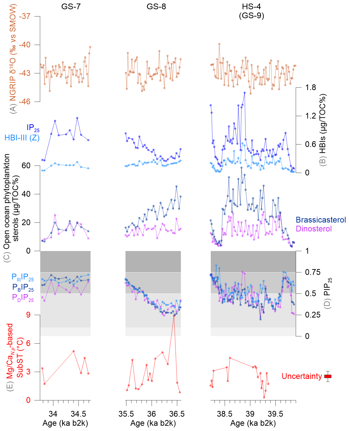
Figure 2 Comparison of biomarker results from MD99-2304 across HS-4, GS-8, and GS-7 (Wong et al., 2025a). (A) NGRIP δ¹⁸O (North Greenland Ice Core Project members, 2004; Andersen et al., 2006), (B) IP₂₅ and HBI-III (Z), (C) brassicasterol and dinosterol, (D) PIP₂₅, and (E) SubST reconstruction from Mg $/$ Ca_N.p (Wong et al., 2025b), with uncertainty range (±0.32 °C) following Elderfield and Ganssen (2000). The boxes in the PIP₂₅ indices signal different sea ice conditions (from darkest to lightest grey: 0.75–1 extensive sea ice, 0.5–0.75 seasonal ice/stable ice edge, 0.1–0.5 little but variable ice extent, 0–0.1 ice-free) (Xiao et al., 2015; Stein et al., 2017).

In contrast to HS-4, biomarker concentrations and PIP₂₅ indices during GS-8 show clear trends with few fluctuations. IP₂₅ concentrations increased from low values, while brassicasterol concentrations decreased from high values following the end of the preceding GI-8. HBI-III (Z) and dinosterol concentrations remained stable. These trends lead to a steady increase in PIP₂₅ indices from ca. 0.3 to 0.7 throughout GS-8. SubSTs varied between 1 and 9 °C during GS-8, with lower temperatures corresponding to higher PIP₂₅ indices (Fig. 2).

The conditions during GS-7 were less variable than those in the other two GSs. IP₂₅ concentrations were overall high, while phytoplankton biomarker concentrations remained stably low. PIP₂₅ indices stayed constant at ca. 0.6. Most of the SubSTs during GS-7 were around 3–6 °C, with the higher values seen early in GS-7 (Fig. 2).

4.2 Greenland Interstadials

As seen for the GSs, proxy records from the eastern Fram Strait indicate that the development, amplitude, and frequency of variations differed both within individual GIs and among different GIs. Both the investigated GIs (GI-8 and GI-7) can be divided into two periods based on changes in biomarker concentrations and PIP₂₅ indices. However, the patterns within each period are not comparable. The highest and most variable HBI concentrations occurred during the first half of GI-8, while sterol concentrations became more variable during the second half of GI-8. This results in higher but fluctuating PIP₂₅ indices in the first half of GI-8, followed by more stable yet lower PIP₂₅ indices in the second half (Wong et al., 2024). SubSTs during GI-8 are reconstructed at a low temporal resolution due to the scarcity of planktonic foraminifera. The available data indicates low SubSTs around 0–3 °C at the onset of GI-8, while the temperatures varied between 3 and 6 °C during the mid to late stages of GI-8 (Fig. 3).

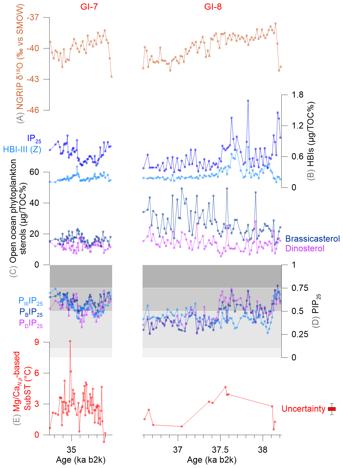
Figure 3 Comparison of biomarker results from MD99-2304 across GI-8 and GI-7 (Wong et al., 2025a). (A) NGRIP δ¹⁸O (North Greenland Ice Core Project members, 2004; Andersen et al., 2006), (B) IP₂₅ and HBI-III (Z), (C) brassicasterol and dinosterol, (D) PIP₂₅, and (E) SubST reconstruction from Mg $/$ Ca_N.p (Wong et al., 2025b), with uncertainty range (±0.32 °C) following Elderfield and Ganssen (2000). The boxes in the PIP₂₅ indices relate to different sea ice conditions (from darkest to lightest grey: 0.75–1 extensive sea ice, 0.5–0.75 seasonal ice/stable ice edge, 0.1–0.5 little but variable ice extent, 0–0.1 ice-free) (Xiao et al., 2015; Stein et al., 2017).

In contrast to GI-8, PIP₂₅ indices present a decline during the first half of GI-7 and a shift toward higher values in the second half. Overall, PIP₂₅ indices were in general higher during GI-7 than in GI-8. This is due to differences in biomarker concentrations. IP₂₅ concentrations decreased and remained low during the first half of GI-7, followed by an increase in the second half. HBI-III (Z) concentrations were slightly higher initially but then decreased slowly during both halves of GI-7. Although sterol concentrations remained generally low throughout GI-7, they also display a two-phase pattern, with an initial increase in the first half succeeded by a gradual decrease in the second half. Moreover, SubSTs exhibit a similar two-phase trend to that of the biomarker concentrations, first increasing and then decreasing, with a turning point occurring at mid-GI-7 (35.1 ka b2k) (Fig. 3).

5 Discussion

The new proxy-based reconstruction from MD99-2304 show that the SIE and SubSTs varied between each GS in the eastern Fram Strait. In the same way, the progression of SIE and SubSTs differed between the investigated GIs (Fig. 4). Within individual GSs and GIs, SIE and SubSTs in the eastern Fram Strait were also less stable than previously assumed (Fig. 4). When considered alongside existing sea ice records from an eastern Nordic Seas transect (Sadatzki et al., 2018, 2020; El bani Altuna et al., 2024b), our SIE and SubST reconstructions highlight the distinctly different sea ice conditions in the northernmost Nordic Seas, differences that cannot be attributed to a higher temporal resolution relative to other records. These findings reveal that glacial sea ice conditions in the eastern Fram Strait differed from those in the southeastern Nordic Seas (Fig. 4).

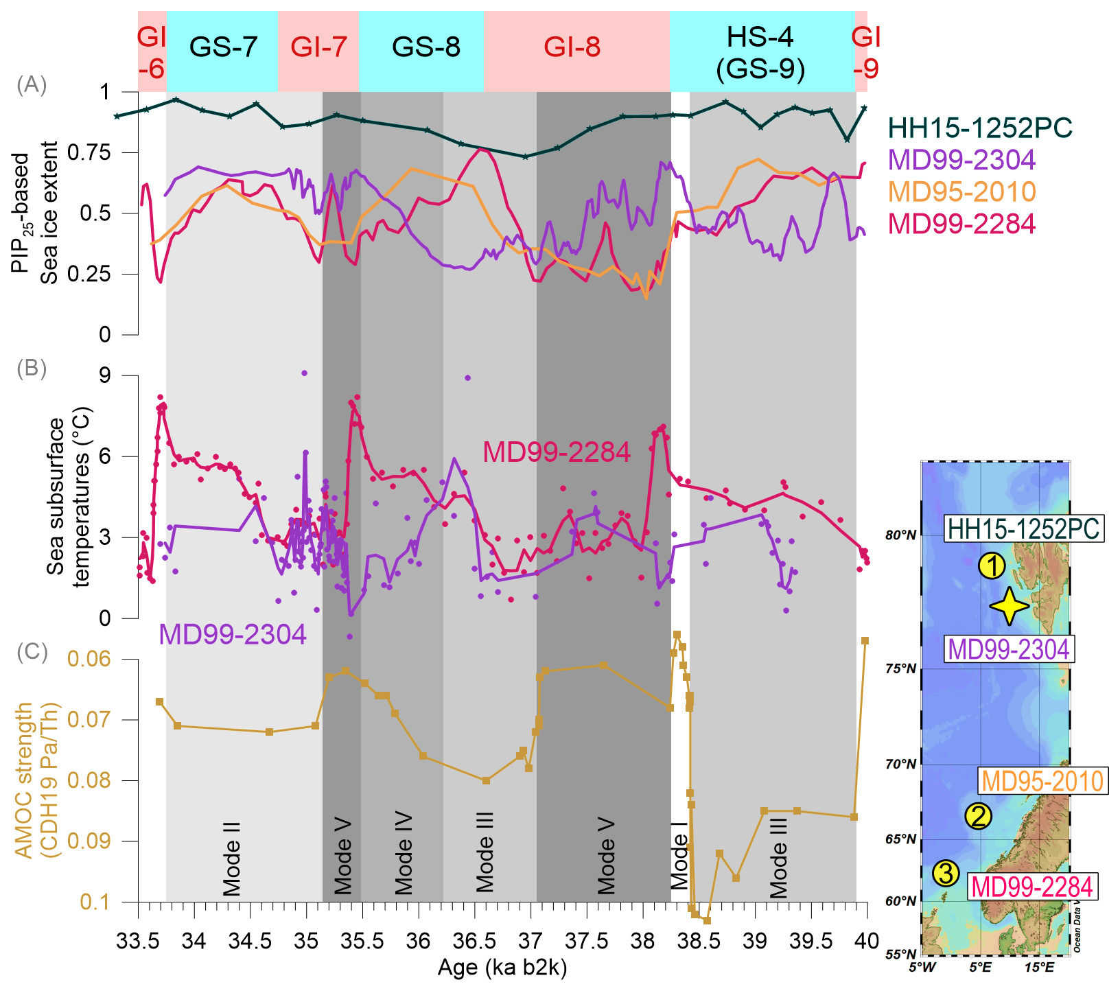
Figure 4 Comparison of sea surface and subsurface conditions between the southeastern and northern Nordic Seas. (A) PIP₂₅-based sea ice extent (SIE) reconstructions from HH15-1252PC (P_IIIIP₂₅; El bani Altuna et al., 2024b), MD99-2284 (P_BIP₂₅ smoothed; Sadatzki et al., 2018), MD95-2010 (P_BIP₂₅ smoothed; Sadatzki et al., 2020), and MD99-2304 (P_BIP₂₅ smoothed; Wong et al. (2025a)). (B) Sea subsurface temperatures (SubSTs) from MD99-2284 (smoothed, estimated using the maximum likelihood transfer function on planktonic foraminifera census counts; Dokken et al., 2013 and Sadatzki et al., 2018) and MD99-2304 (smoothed, based on Mg $/$ Ca_N.p; Wong et al. (2025b)). PIP₂₅ indices relate to different sea ice conditions (0.75–1 extensive sea ice, 0.5–0.75 seasonal ice/stable ice edge, 0.1–0.5 little but variable ice extent, 0–0.1 ice-free) (Xiao et al., 2015; Stein et al., 2017). The sites, numbered consistently with Fig. 1, are illustrated on the map in the right corner using Ocean Data View (Schlitzer, Reiner, Ocean Data View, https://odv.awi.de/, 2025). The SIE and SubST datasets are compared with (C) AMOC strength records (based on Pa $/$ Th) from the Bermuda Rise (Core CDH19) (Henry et al., 2016b). Lower Pa $/$ Th ratios indicate a stronger AMOC (e.g., Bradtmiller et al., 2014; Robinson et al., 2019; Missiaen et al., 2020). Blue and red boxes indicate Greenland Stadials (GSs) and Interstadials (GIs), respectively. Boxes shaded from white to dark grey illustrate Modes I to V. All smoothed lines are derived using a 3-point moving average. The original SubST data are marked with red round symbols.

We hypothesize that shifts in oceanic heat distribution driven by variations in large-scale ocean circulation, regulated SIE and SubSTs in the eastern Nordic Seas during the investigated period. One of the key drivers of modern Arctic SIE variations is the large-scale ocean circulation and heat transport (e.g., Polyakov et al., 2017; Docquier and Koenigk, 2021; Docquier et al., 2022). Anomalies in ocean heat transport into the Nordic Seas originate in the subpolar North Atlantic (Årthun and Eldevik, 2016), with the AMOC and the subpolar gyre (SPG) component contributing equally to the heat transport when crossing the Greenland-Scotland Ridge (Rhein et al., 2011; Li and Born, 2019).

However, due to the lack of SPG component reconstructions, we use the existing AMOC reconstruction (Fig. 4C) (Henry et al., 2016b) as a proxy for ocean heat transport to the Nordic Seas. Modeling studies (Sun et al., 2021; Jones et al., 2024), observational data (Mandal et al., 2024) and combined approaches (Rhein et al., 2011) indicate that SPG and AMOC strengths are correlated on multidecadal timescales. Therefore, in this study, we assume that ocean heat transport into the Nordic Seas is linked to the strength of the AMOC (Day et al., 2012; Årthun et al., 2019; van der Linden et al., 2019). Based on SIE and SubSTs from MD99-2304 and previously published sites in the southeastern Nordic Seas (Sadatzki et al., 2018, 2020), complemented by the Pa $/$ Th-based AMOC reconstruction by Henry et al. (2016b), we define five modes of variability that characterize the observed dynamic interplay between ocean circulation, ocean temperatures, and sea ice conditions (Figs. 4 and 5). Sedimentary Pa $/$ Th is considered a proxy for past ocean circulation strength (e.g., Bradtmiller et al., 2014; Robinson et al., 2019; Missiaen et al., 2020). In this study, we use Pa $/$ Th values of < 0.065, 0.065–0.075, and > 0.075 to correspond to strong, intermediate, and weak AMOC strengths, respectively.

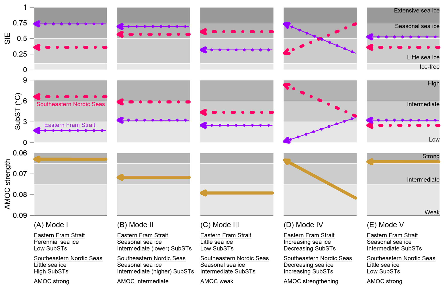
Figure 5 Schematic illustration of the relationships between AMOC strength and the eastern Nordic Seas SIE and SubSTs. Five modes are identified: (A) Mode I, (B) Mode II, (C) Mode III, (D) Mode IV, and (E) Mode V. The purple lines with diamonds represent records from MD99-2304 in the eastern Fram Strait, and the magenta dashed lines represent records from MD99-2284 and MD95-2010 in the southeastern Nordic Seas. The boxes in the PIP₂₅ indices relate to different sea ice conditions (from darkest to lightest grey: 0.75–1 extensive sea ice, 0.5–0.75 seasonal ice/stable ice edge, 0.1–0.5 little but variable ice extent, 0–0.1 ice-free) (Xiao et al., 2015; Stein et al., 2017). SubSTs are classified into three categories: high (> 6 °C, dark grey box), intermediate (3–6 °C, medium grey box), and low (< 3 °C, light grey box). AMOC strength is inferred from Pa $/$ Th values. Pa $/$ Th< 0.065 is considered to indicate strong AMOC (dark grey box), 0.065–0.075 intermediate AMOC (medium grey box), and > 0.075 weak AMOC (lightest grey box).

Of the identified modes, Modes I and IV occurred during GSs, Mode V during GIs, and Modes II and III during both. We argue that the interaction between surface and subsurface ocean heat content in the southeastern Nordic Seas, influenced by the strength of the AMOC, played a key role in shaping sea ice conditions in the northernmost Nordic Seas. These modes reflect a dynamic interplay among AMOC strength, SubSTs, and SIE in the eastern Nordic Seas. Given that Modes III and V recurred within the limited period investigated, and Modes II and III spanned both GS and GI (Fig. 4), we consider it likely that these modes represent inherent physical processes of the Earth system. However, due to the constraints of the available records, their broader applicability remains uncertain.

5.1 Mode I: strong oceanic heat release in the southeastern Nordic Seas

Mode I (Fig. 5A), occurring toward the end of HS-4, is characterized by a perennial sea ice cover (Wong et al., 2024) and low SubSTs in the eastern Fram Strait, corresponding with little SIE and high SubSTs in the southeastern Nordic Seas (Sadatzki et al., 2018, 2020). Meanwhile, the AMOC is defined to be strong, based on a Pa $/$ Th value < 0.065 (Figs. 4 and 5A).

The presence of perennial sea ice in the eastern Fram Strait is documented by low biomarker concentrations from MD99-2304. Although PIP₂₅ indices are high, they still underestimate SIE due to these low biomarker concentrations (Fig. 2) (Wong et al., 2024). Biomarker records from HH15-1252PC, located northwest of MD99-2304 in the northeastern Fram Strait, also indicate perennial sea ice (El bani Altuna et al., 2024b). However, little SIE is observed in the southeastern Nordic Seas (MD95-2010 and MD99-2284), with the sea ice margin reaching the Vøring Plateau (MD95-2010) (Sadatzki et al., 2018, 2020) (Fig. 4A). During this mode, the inflow of AW likely intensified due to a strong AMOC. Sea ice is sensitive to both surface and subsurface ocean heat content (Polyakov et al., 2017; Docquier and Koenigk, 2021; Docquier et al., 2022). When the strong AW inflow reached the surface, it likely played a key role in preventing sea ice formation in the southeastern Nordic Seas.

Differences in temperature reconstructions further support these sea ice patterns. Low SubSTs in the eastern Fram Strait are suggested by low temporal resolution Mg $/$ Ca-based temperature reconstructions (Mg $/$ Ca_N.p). In the southeastern Nordic Seas (MD99-2284), a foraminiferal transfer function-based temperature reconstruction presents high SubSTs (Sadatzki et al., 2018) (Fig. 4B). Throughout the investigated period, 40–33.5 ka b2k, atmospheric temperatures were substantially lower than ocean temperatures (≤ −35 °C) (Kindler et al., 2014). Due to the strong ocean-atmosphere temperature gradient, oceanic heat transported by the AW was rapidly released to the atmosphere in ice-free areas south of the Vøring Plateau, as supported by the comparison of the southeast and northeast Nordic Seas SubST records (Figs. 4B and 5A). Before reaching the sea ice margin in the Vøring Plateau, the AW cooled enough to submerge, allowing sea ice to cover the northern Nordic Seas as far south as the Vøring Plateau (Fig. 6A).

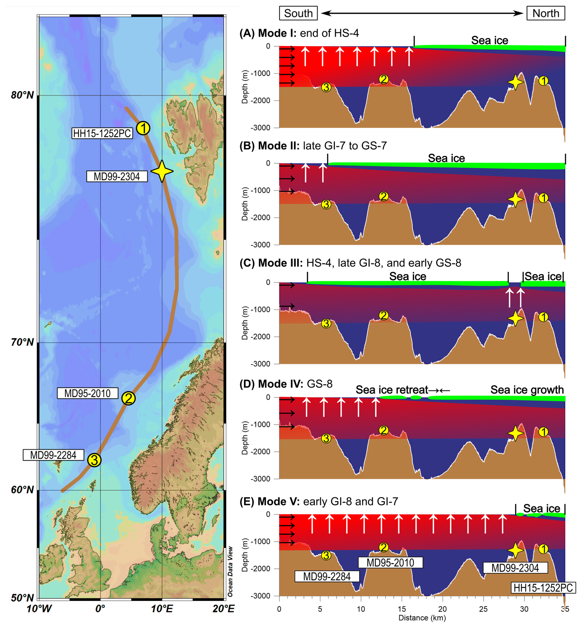
Figure 6 Schematic illustrating the relationship between the AMOC strength and SIE along the eastern Nordic Seas transect under five modes: (A) Mode I – strong AMOC and perennial sea ice in the north, (B) Mode II – intermediate AMOC strength and seasonal sea ice, (C) Mode III – weak AMOC and polynyas in the north, (D) Mode IV – strengthening AMOC and increasing sea ice in the north, and (E) Mode V – strong AMOC and seasonal sea ice in the north. The transect is indicated by the brown line in the left panel. The black rightward arrows indicate the AW and oceanic heat inflow, while the white upward arrows represent ocean heat release. The gradient from red to transparent shows oceanic heat loss in the AW. A green layer on the ocean surface denotes sea ice cover. Bathymetry along the transect is obtained from GEBCO and processed using QGIS. The map is produced with Ocean Data View (Schlitzer, Reiner, Ocean Data View, https://odv.awi.de/, 2025).

5.2 Mode II: reduced heat transport and sea ice buildup across the eastern Nordic Seas

Mode II (Fig. 5B), taking place during late GI-7 and the subsequent GS-7, represents periods when seasonal sea ice dominated both the eastern Fram Strait and the southeastern Nordic Seas. SubSTs were at intermediate levels in both the north and south (Sadatzki et al., 2018, 2020). SIE and SubSTs show reduced contrasts between the north and south compared to Mode I (Fig. 5A and B). During this mode, the AMOC remained at an intermediate strength, with Pa $/$ Th values between 0.065 and 0.075 (Figs. 4 and 5B).

The Mode II seasonal, nearly extensive sea ice in the eastern Fram Strait is supported by high IP₂₅, low HBI-III (Z), low sterol concentrations, and high PIP₂₅ indices (Stein et al., 2017; Köseoğlu et al., 2018) (Figs. 2 and 3). Perennial sea ice persisted at HH15-1252PC (El bani Altuna et al., 2024b). Further south, seasonal sea ice expanded into the southeastern Nordic Seas (Sadatzki et al., 2018, 2020) (Fig. 4A). During this mode, an AMOC of intermediate strength likely reduced the oceanic heat transported via the AW inflow into the Nordic Seas, compared to the stronger AMOC state observed in Mode I.

Temperature reconstructions suggest intermediate Mg $/$ Ca_N.p-based SubSTs in the eastern Fram Strait (MD99-2304), though the lack of continuous data prevents a more precise interpretation. In the southeastern Nordic Seas (MD99-2284), foraminiferal transfer function-based SubSTs were also at intermediate levels but remained higher than those from the eastern Fram Strait during this mode (Sadatzki et al., 2018, 2020) (Fig. 4B). The reduction in oceanic heat, indicated by the lowered SubSTs at MD99-2284 (Sadatzki et al., 2018) (Fig. 5A and B), was insufficient to trigger a year-round retreat of sea ice in the southeastern Nordic Seas. As a result, the region remained seasonally ice-covered, with more sea ice accumulating farther north (Fig. 4A). Although seasonal cycles are expected, the AW submerged beneath the sea ice cover and halocline before reaching the Faeroe-Shetland Channel. This allowed heat to accumulate at intermediate depths across the Nordic Seas (e.g., Rasmussen and Thomsen, 2004; Dokken et al., 2013; Ezat et al., 2014; Sessford et al., 2019) (Fig. 6B).

The relatively small difference in SubSTs between the southeastern (MD99-2284) and northern Nordic Seas (MD99-2304), compared to Mode I, indicates that oceanic heat was more evenly distributed at intermediate depths within the Nordic Seas. Only slight heat loss occurred between the north and south (Figs. 4B and 5B). This supports the hypothesized existence of a homogeneous intermediate water mass occupying the Nordic Seas during GSs (Sessford et al., 2019). Mode II can thus be interpreted as the most representative of expected GS conditions in the eastern Nordic Seas among all five modes, consistent with previous studies (Dokken et al., 2013; Sadatzki et al., 2019, 2020; Sessford et al., 2019). Note that, while this interpretation aligns with the suggested AMOC mechanisms, the existing AMOC reconstruction (Henry et al., 2016b) (Fig. 4C) lacks sufficient temporal resolution during GI-7 to provide direct support.

5.3 Mode III: oceanic heat reservoir in the south and polynyas in the north

Mode III (Fig. 5C), occurring during HS-4, late GI-8, and early GS-8, features little SIE and low SubSTs in the eastern Fram Strait, while the southeastern Nordic Seas experienced seasonal sea ice and intermediate SubSTs (Sadatzki et al., 2018, 2020). The AMOC was weak during this mode, based on Pa $/$ Th values > 0.075 (Figs. 4 and 5C).

In the eastern Fram Strait, nearly ice-free conditions are reflected by varying HBI, high sterol concentrations, and consistently low PIP₂₅ indices from MD99-2304 (Stein et al., 2017; Köseoğlu et al., 2018) (Figs. 2 and 3). This evidence points to repeated polynya activity in the eastern Fram Strait (Wong et al., 2024), since perennial sea ice was suggested to have covered the Vøring Plateau and areas to its north (Sadatzki et al., 2019, 2020). However, the polynyas observed at MD99-2304 were likely small and local in extent since the biomarker records from the nearby HH15-1252PC document persistent perennial sea ice (Fig. 4A) (El bani Altuna et al., 2024b).

A weak AMOC during this mode led to reduced oceanic heat into the Nordic Seas. Foraminiferal transfer function-based SubSTs reached intermediate levels in the southeastern Nordic Seas, which were lower than those during Modes I and II (Sadatzki et al., 2018) (Fig. 4B). This reflects lower ocean heat contents in the southeastern Nordic Seas compared to the first two modes. Meanwhile, Mg $/$ Ca_N.p-based SubSTs remained low in the eastern Fram Strait (Fig. 4B). The contrast with the higher SubSTs in the southeastern Nordic Seas (Fig. 5C) suggests oceanic heat depletion in the eastern Fram Strait.

During Mode III, the AW submerged beneath the extensive sea ice in the southeastern Nordic Seas. Despite the overall reduction in northward ocean heat transport, heat still accumulated beneath the sea ice and halocline in this region. This heat content was then transported at intermediate depths along the NwAC pathway, forming a heat reservoir within the well-stratified eastern Nordic Seas (e.g., Rasmussen and Thomsen, 2004; Dokken et al., 2013; Ezat et al., 2014; Sessford et al., 2019).

While stratification remained strong in the eastern Nordic Seas, vertical mixing still occurred in its interior. One of the primary drivers of vertical mixing is the kinetic energy from variations in internal waves (Ferrari and Wunsch, 2009). Increased vertical mixing can enhance the exchange of heat and salt between ocean layers (e.g., Liang and Losch, 2018; Beer et al., 2023; Saenz et al., 2023), hence, the warmer, saltier AW can be brought from intermediate depths to the surface, destabilizing the halocline on small spatial scales (e.g., Nguyen et al., 2009; Lind et al., 2016; Rheinlænder et al., 2021). Since sea ice is sensitive to changes in surface and subsurface temperatures (Polyakov et al., 2017; Docquier and Koenigk, 2021; Docquier et al., 2022), upward heat fluxes can thus contribute to sea ice loss (e.g., Beer et al., 2023; Saenz et al., 2023). Additionally, the much steeper continental slope in the eastern Fram Strait (Fig. 1), relative to the Vøring Plateau, may have played a key role in breaking internal waves (Falk-Petersen et al., 2015; Zhang et al., 2022). This process likely caused an upwelling of accumulated oceanic heat from the AW entering the eastern Fram Strait, thereby contributing to subsurface heat depletion and facilitating sea ice loss at MD99-2304 (Fig. 6C). The same polynya response is not observed further north at HH15-1252PC, likely due to the gentler bathymetry (Fig. 1). Wong et al. (2024) argued that the polynyas were more likely formed by sensible heat flux from below, rather than driven by katabatic winds, due to the lack of evidence for a large Svalbard-Barents Sea Ice Sheet capable of triggering strong katabatic winds.

Hence, persistent sea ice cover and submerged AW inflow in the southeastern Nordic Seas likely contributed to the buildup of an ocean heat reservoir at intermediate depths under a weak AMOC. We argue that vertical mixing in the eastern Fram Strait, possibly driven by interactions between internal waves and the steep continental slope, caused upwelling of stored heat. This process destabilized the halocline and eventually triggered the formation of seasonal polynyas at MD99-2304 during these periods, as discussed in Wong et al. (2024). Furthermore, polynya activity at MD99-2304 is absent during GS-7, which instead experienced Mode II, characterized by a seasonal sea ice cover in the eastern Nordic Seas under an AMOC of intermediate strength.

5.4 Mode IV: strengthening ocean heat transport and increasing northern sea ice

Mode IV (Fig. 5D) displays a trend of increasing SIE and decreasing SubSTs in the eastern Fram Strait, following Mode III when polynyas were present. This mode is observed during GS-8. In contrast, in the southeastern Nordic Seas, SIE decreased and SubSTs increased (Sadatzki et al., 2018, 2020). During this mode, the AMOC continued to strengthen, with Pa $/$ Th values decreasing from > 0.075 to < 0.065 (Figs. 4 and 5D).

Starting with nearly ice-free conditions, the eastern Fram Strait saw a rise in SIE, as indicated by increasing IP₂₅ and decreasing sterol concentrations, along with increasing PIP₂₅ values (Stein et al., 2017; Köseoğlu et al., 2018) (Figs. 2 and 4). In the meantime, a perennial sea ice cover dominated at HH15-1252PC (El bani Altuna et al., 2024b). In contrast, biomarker records from the southeastern Nordic Seas show an opposite trend, with SIE continuously decreasing (Sadatzki et al., 2018, 2020) (Fig. 4A). Mg $/$ Ca_N.p-based SubSTs gradually decreased in the eastern Fram Strait, while foraminiferal transfer function-based SubSTs continued to rise in the southeastern Nordic Seas (Sadatzki et al., 2018) (Fig. 4B).

A strengthening AMOC gradually intensified northward ocean heat transport. This increased heat content, as evidenced by the rising SubSTs at MD99-2284, entailed a gradual reduction in SIE in the southeastern Nordic Seas (Sadatzki et al., 2018, 2020) (Fig. 4 and 5D). As sea ice gradually disappeared from the region, the AW reached the surface (Dokken et al., 2013; Sadatzki et al., 2019), releasing progressively more oceanic heat to the colder atmosphere.

Sufficient ocean heat was lost in the southeastern Nordic Seas for the AW to be dense enough to submerge before reaching the eastern Fram Strait. Thereby, the coupled process of heat loss south of the Fram Strait and AW deepening contributed to gradual sea ice accumulation and decreasing SubSTs in the high north (Fig. 6D).

5.5 Mode V: strong northward ocean heat transport and sea ice retreat

Mode V (Fig. 5E) is marked by seasonal sea ice and intermediate SubSTs in the eastern Fram Strait, and little SIE with low SubSTs in the southeastern Nordic Seas during early GI-8 and GI-7 (Sadatzki et al., 2018, 2020). The AMOC strength was strong, comparable to Mode I (Pa $/$ Th < 0.065) (Figs. 4 and 5E).

Low HBI, high sterol concentrations and low PIP₂₅ indices at MD99-2304 suggest the presence of seasonal sea ice (Stein et al., 2017; Köseoğlu et al., 2018). Conversely, biomarker evidence from HH15-1252PC in the northeastern Fram Strait indicates an extensive sea ice cover (Fig. 4A) (El bani Altuna et al., 2024b), pointing to a sea ice margin between the two core sites. In the southeastern Nordic Seas, biomarker records indicate nearly ice-free conditions (Sadatzki et al., 2018, 2020) (Fig. 4A). Combined, these findings imply a substantial seasonally ice-free area along the eastern Nordic Seas, extending into the eastern Fram Strait.

Mg $/$ Ca_N.p-based SubSTs at MD99-2304 averaged slightly above 3 °C, the boundary between intermediate and low levels defined in this study. Foraminiferal transfer function-based SubSTs were slightly lower than 3 °C at MD99-2284 (Sadatzki et al., 2018) (Fig. 4B). Overall, SubSTs show little contrast between the two regions.

The strong AMOC during these periods intensified the northward inflow of heat-laden AW. In ice-free areas, oceanic heat was transferred to the surface along with the warm AW, leaving little heat in the subsurface, as indicated by low SubSTs in the southeastern Nordic Seas (MD99-2284) (Sadatzki et al., 2018) and the eastern Fram Strait (MD99-2304) (Figs. 4B and 5E). This heat content was efficiently released to the atmosphere, accelerating atmospheric warming, with barely any sea ice to disrupt heat exchange. Once the atmospheric temperature reached a critical threshold, sea ice formation across the eastern Nordic Seas can be further inhibited, thus creating a positive feedback loop. facilitate the release of oceanic heat into the atmosphere.

Among all modes investigated, this mode (Fig. 5E) most closely resembles modern-day surface and subsurface conditions in the eastern Nordic Seas. Modern oceanographic observations from this region support the presence of similar physical processes (e.g., Schlichtholz, 2011; Alexeev et al., 2017; Smedsrud et al., 2022). Both the reconstructed and modern systems are characterized by a large ice-free surface, intense AW inflow, a weak halocline, and active vertical mixing in the upper ocean (Fig. 6E).

5.6 Other mechanisms

In addition to changes in ocean circulation, SIE in the Nordic Seas may have been influenced by prevailing atmospheric conditions, including atmospheric temperature changes and wind patterns. Records from Greenland indicate that atmospheric temperatures display a comparable pattern of variability between and within individual GSs and GIs (Kindler et al., 2014; Rasmussen et al., 2014). SIE variability in the southeastern Nordic Seas (Sadatzki et al., 2019, 2020) and the North Atlantic (Scoto et al., 2022) aligns with the cycles observed in the D-O climate oscillations.

However, sea ice reconstructions from the southeastern Nordic Seas (Sadatzki et al., 2019, 2020), synchronized with Greenland records through the identification of microtephra layers (Berben et al., 2020), show that sea ice changes in the Faroe-Shetland Channel preceded shifts in atmospheric temperatures over Greenland. This suggests that the atmospheric temperature changes were driven by sea ice variations, rather than the other way around.

Furthermore, since no reconstructions provide information on changing wind patterns or wind strengths for the investigated time interval, our study focuses on understanding the role of ocean circulation.

6 Conclusions

Our new proxy results from MD99-2304 reveal clear variability in SIE and SubSTs in the eastern Fram Strait, both between and within individual GSs and GIs, during the period between 40 and 33.5 ka b2k. The proxy signals recorded in MD99-2304 during these GSs and GIs differed from the regularly repetitive GS-GI oscillations observed in the Greenland ice cores and southeastern Nordic Seas reconstructions. This indicates that the local variability in SIE and the associated release of oceanic heat observed in the eastern Fram Strait had a minor impact on climate conditions over Greenland during GSs and GIs. Our records support previous studies suggesting that atmospheric changes over Greenland were driven by changes in sea ice conditions in the southeastern Nordic Seas and the North Atlantic (Jansen et al., 2020; Sadatzki et al., 2020; Buizert et al., 2024).The variability observed specifically at site MD99-2304 was likely caused by a combined influence of oceanic heat distribution and local topography (Fig. 1), which was not present at HH15-1252PC (El bani Altuna et al., 2024a, b), a site northwest of our site in the eastern Fram Strait. Interaction between internal waves and the steep continental slope at MD99-2304 may have triggered upwelling of the warm AW, bringing oceanic heat to the surface.

Fluctuations in SIE and SubSTs in the eastern Fram Strait were primarily driven by northward oceanic heat transport, which was strongly influenced by the strength of the AMOC and sea ice conditions in the southeastern Nordic Seas. Based on these findings, we identify five distinct modes describing the interplay between SIE, SubSTs, and AMOC strength across the eastern Nordic Seas.

Except for GS-7, all other GSs and GIs during the investigated period experienced multiple modes of variability. Modes I, IV, and V confined within a single GS or GI, while Modes II and III persisted from a GI into a GS. These results document more variable sea ice conditions in the northernmost Nordic Seas than the previous conceptualizations (Dokken et al., 2013; Sadatzki et al., 2019, 2020; El bani Altuna et al., 2024a), which had suggested that the region was permanently covered by sea ice throughout all GSs and GIs. Our new findings indicate that the seasonally ice-free conditions at MD99-2304 during HS-4 and GI-8, identified by Wong et al. (2024), were not a unique example of more variable glacial conditions in the eastern Fram Strait.