H11 meltwater and standard 127 ka Last Interglacial simulations suggest more modest peak temperatures for both Greenland and Antarctica: a multi-model study of water isotopes

The Last Interglacial (LIG) period, approximately 130 000 to 115 000 years ago, represents one of the warmest intervals of the past 800 000 years. Here, we simulate water isotopes in precipitation over Antarctica and the Arctic during the LIG, using three isotope-enabled atmosphere–ocean coupled climate models: HadCM3, MPI-ESM-wiso, and GISS-E2.1. These models were run following the Paleoclimate Modelling Intercomparison Project phase 4 (PMIP4) protocol for the LIG at 127 ka (kiloyears ago), supplemented by a 3000-year Heinrich Stadial 11 (H11) experiment using HadCM3. The long H11 simulation applies Northern Hemisphere meltwater to the North Atlantic, causing large-scale changes in ocean circulation – including cooling in the North Atlantic and Arctic and warming in the Southern Ocean and Global Ocean. While the standard 127 ka simulations do not capture the observed Antarctic warming and sea ice reduction in the Southern Ocean and Antarctic regions, they do capture around half of the warming in the Arctic. The H11 simulations align more closely with observations than the 127 ka simulations. H11 captures more than 80 % of the warming, sea ice loss, and δ¹⁸O changes for both Greenland and Antarctica. Decomposition of seasonal δ¹⁸O drivers highlights the dominant role of sea ice retreat and associated changes in precipitation seasonality in influencing isotopic values across all simulations, alongside a smaller common response to orbital forcing. We use the H11 and multi-model 127 ka simulations together to infer LIG surface air temperature (SAT) changes based on ice core measurements. The peak inferred LIG Greenland SAT increase is $+\mathrm{2.89}\pm \mathrm{1.32}$ K at the NEEM ice core site – less than half the previously inferred warming. Peak inferred LIG Antarctic SAT increases are $+\mathrm{4.39}\pm \mathrm{1.45}$ K at EDC, dropping to $+\mathrm{1.67}\pm \mathrm{3.67}$ K at TALDICE. These calculated warming values reflect climate effects alone and do not account for any ice-flow- or site-elevation-related impacts. Coastal sites in Greenland and Antarctica appear to have experienced less warming compared with higher central regions.

1 Introduction

The Last Interglacial (LIG) period, or Eemian, occurring approximately 130 000 to 115 000 years ago, stands out as one of the warmest interglacials in palaeoclimate records over the past 800 000 years (Past Interglacials Working Group of PAGES, 2016). The globe experienced temperatures higher than pre-industrial levels during peak LIG conditions (Hoffman et al., 2017; Fischer et al., 2018). Estimates of global-mean maximum surface air temperature LIG warming of 0.8 ± 0.5 K above pre-industrial levels are supported by Hoffman et al. (2017), Fischer et al. (2018), and Shackleton et al. (2020). The magnitude of warming was greater in polar and subpolar regions compared to the global-mean value (CAPE-Last Interglacial Project Members, 2006; Sime et al., 2009; Capron et al., 2014, 2017). Sime et al. (2023) estimated the Arctic-wide summer surface air temperature warming at 127 ka to be 3.7 ± 1.5 K, when the Arctic may have been sea-ice-free during summer (Guarino et al., 2020; Vermassen et al., 2023), whilst Greenland surface temperatures as high as 8 ± 4 K warmer than the PI have been posited by NEEM community members (2013). Similarly, peak LIG annual-mean warming over central Antarctic ice core sites of +3–6 K has been suggested (e.g. Jouzel et al., 2007; Sime et al., 2009; Otto-Bliesner et al., 2013; Bakker et al., 2014; Capron et al., 2014).

Alongside the increases in polar surface air temperatures, sea ice cover was reduced and sea surface temperature warmed across the Arctic Ocean and Southern Ocean at 127–128 ka compared to the pre-industrial period (Holloway et al., 2017; Chadwick et al., 2023). Recently Vermassen et al. (2023) used open water species, found in Arctic marine cores, to suggest that the Arctic was likely seasonally sea-ice-free during the LIG, though Arctic age models are currently characterized by significant uncertainty (Razmjooei et al., 2023). This supports the idea that sea ice feedbacks were important in amplifying the Arctic LIG warming (Guarino et al., 2020; Diamond et al., 2021, 2023). In the Southern Ocean work on diatom fossil assemblages in marine sediment cores and sea-salt sodium in Antarctic ice cores helps underpin our understanding of Antarctic sea ice (Wolff et al., 2006; Crosta et al., 2022; Chadwick et al., 2020, 2021, 2022). Gao et al. (2025) examined four recent Southern Ocean core syntheses (from Capron et al., 2017; Hoffman et al., 2017; Chandler and Langebroek, 2021a; Chadwick et al., 2021) and estimated a Southern Ocean annual SST anomaly of around +1.3 K at 127 ka.

Whilst the Arctic summer warmth and loss of sea ice during the LIG can be attributed mainly to orbital forcing (Guarino et al., 2020; Diamond et al., 2023; Sime et al., 2023; Vermassen et al., 2023), the reduced sea ice and warmer Southern Ocean is not attributable to either orbital or greenhouse gas forcing, as austral summer solar insolation was lower and greenhouse gas concentrations were below pre-industrial levels at 127 ka (Berger and Loutre, 1991; Otto-Bliesner et al., 2017). Although the Antarctic ice sheet volume and configuration remain poorly constrained (Golledge et al., 2021), modelling studies nevertheless show that a smaller-than-pre-industrial ice sheet alone is very unlikely to account for the estimated LIG sea ice loss and Southern Ocean warming (Holloway et al., 2016; Hutchinson et al., 2024). Alongside this, recent simulations run according to the standard Paleoclimate Modelling Intercomparison Project (PMIP) LIG protocol (Otto-Bliesner et al., 2017), which applies 127 ka orbital and greenhouse gas forcing, also do not fully replicate the pronounced warmth at southern mid-to-high latitudes (Lunt et al., 2013; Otto-Bliesner et al., 2017, 2021; Kageyama et al., 2021). This model–observation mismatch may be due to the models not capturing a prolonged period of meltwater influx from the Northern Hemisphere ice sheet melt and subsequent weakening of the Atlantic Meridional Overturning Circulation with warming of the south due to the bipolar seesaw effect (Holloway et al., 2018; Sime et al., 2019a; Chadwick et al., 2023; Gao et al., 2025).

From approximately 132 to 128 ka, in the period before peak LIG warmth, meltwater entered the North Atlantic from the deglaciation of the large Northern Hemisphere glacial-period ice sheets. The event is sometimes called Heinrich 11 (H11), although technically a Heinrich event is defined as the occurrence of very significant meltwater markers (e.g. ice-rafted debris) in North Atlantic sediment cores (Heinrich, 1988; Hemming, 2004), rather than being a simple label for the period marked by Northern Hemisphere meltwater entering the oceans. The extra freshwater reduced the thermohaline circulation-driven part of the Atlantic Meridional Overturning Circulation (AMOC) and decreased the associated export and loss of global heat through and to the North Atlantic (Rahmstorf, 2000; Weaver et al., 2003; Clark et al., 2002; McManus et al., 2004). This resulted in large-scale changes in ocean circulation, including cooling in the North Atlantic and Arctic, and warming in the Southern and Global Ocean. Recent dating of the H11 event suggests that the meltwater could have persisted for 3000 to 5000 years (with the length partly depending on definition of “Heinrich”) and that it is possible that the meltwater ceased directly before peak LIG temperatures at both poles (Marino et al., 2015; Stoll et al., 2022).

Given the progress in understanding the processes key to Last Interglacial (LIG) climate at the poles, it seems timely to revisit the question of inferring, or quantifying, polar warming during the LIG from ice core measurements. Ice core stable water isotopes (δ¹⁸O) from Antarctica and Greenland provide invaluable information on past variations in site temperature (EPICA community members, 2004; Jouzel et al., 2007; Sime et al., 2013; Malmierca-Vallet et al., 2018; Domingo et al., 2020). Jouzel et al. (1997) note that linear relationships between the mean annual δ¹⁸O content in precipitation and the mean annual temperature at the precipitation site in polar regions support this use of ice core measurements. However, retrieving accurate LIG peak temperature information from δ¹⁸O values is challenging (e.g. Jouzel et al., 1997, 2003; NEEM community members, 2013; Goursaud et al., 2021). In particular, temporal slopes often appear lower than present-day spatial slopes (Jouzel et al., 1997; Guan et al., 2016).

The most important local-site control on δ¹⁸O in polar precipitation is thought to be the site condensation temperature (Dansgaard, 1954; Jouzel et al., 1997). Lee et al. (2008) and Liu et al. (2023) therefore examine relationships between condensation temperature and inversion layers in Antarctica, as well as the reconciliation of spatial and seasonal δ¹⁸O–temperature relationships, finding relationships of around 1.2 ‰ K⁻¹ between the inversion layer and δ¹⁸O in precipitation.

Additional local-to-regional influences include changes in local boundary layer conditions (e.g. Krinner et al., 1997; Noone and Simmonds, 2002) and the impacts of continental vapour recycling (e.g. Werner et al., 2001; Sjolte et al., 2014).

However, δ¹⁸O is also dependent on the origin of the vapour and its associated pathways and history as it travels to the precipitation site (Dansgaard, 1954; Boyle, 1997; Kindler et al., 2014; Guan et al., 2016). Changes in Greenland δ¹⁸O during climate shifts have been shown to be sensitive to both source properties and pathway changes (Boyle, 1997; Werner and Heimann, 2002), along with key controls such as precipitation seasonality and intermittency. These factors affect Antarctica and Greenland differently due to the nature of precipitation, sea ice, and other geographically specific influences (Werner et al., 2001; Sime et al., 2008, 2013; Münch et al., 2021).

For example, Vinther et al. (2010) and Sjolte et al. (2014) show that local temperature controls on Greenland δ¹⁸O can be weak during summer; this may be partially due to the limited impact of sea ice in summer (e.g. Sime et al., 2013; Sjolte et al., 2014; Sime et al., 2019b). Many recent studies now consider such factors, including air mass trajectories and vapour-to-precipitation distance (e.g. Delaygue et al., 2000; Schlosser et al., 2004), evaporation and ocean surface conditions (e.g. Vimeux et al., 1999), and especially sea ice (e.g. Bertler et al., 2018; Holloway et al., 2016, 2017).

Seminal work by Petit et al. (1999) at Vostok in Antarctica used a δ¹⁸O–temperature relationship of 0.7 ‰ K⁻¹, while in West Antarctica, WAIS Divide Project Members (2015) used a relationship of 0.8 ‰ K⁻¹. For Greenland, at the NEEM core site, NEEM community members (2013) used a value of 0.48 ± 0.1 ‰ K⁻¹.

However, given the timescale-, region-, and climate-shift-dependent controls on δ¹⁸O across Antarctica and Greenland, it is imperative to study the relationships between δ¹⁸O and temperature for each specific climate shift, especially where we seek to infer temperature from measured changes in δ¹⁸O in ice cores (Jouzel et al., 1997).

Isotope-enabled general circulation models (GCMs) allow a more direct comparison of model isotopic outputs with water isotope concentrations measured in natural archives, including ice cores. These models provide the most comprehensive means that we possess to include all the factors that affect the δ¹⁸O and surface air temperature changes (Werner et al., 2001; Werner and Heimann, 2002). They have therefore been used to investigate δ¹⁸O and temperature in polar regions and to provide a theoretical framework that accounts for both spatial and temporal variations in isotopic signals (Werner and Heimann, 2002; Sime et al., 2008). This study investigates water isotope changes in precipitation in the Antarctic and the Arctic regions that occurred between the PI and LIG using three isotope-enabled GCMs and is the first isotopic-enabled multi-model study of the LIG. LIG simulations are run with each of these models according to the recent PMIP4 LIG protocol (Otto-Bliesner et al., 2017). These simulations are supplemented by a long 3000-year H11 experiment which is run using HadCM3. The Methods section (Sect. 2) details these models, experimental set-ups, and ice core δ¹⁸O and climate data, alongside analysis methods. Section 3 presents the results, Sect. 4 discusses the findings, and Sect. 5 concludes the study.

2 Methods

The Methods section details the three water-isotope-enabled models used, simulations run with these models, how model output is handled and analysed, and Antarctic and Greenland ice core δ¹⁸O and the wider set of observations used to evaluate the model simulations.

2.1 Models

The use of three isotope-enabled models aids in understanding the model dependency of the results. The models are the Max Planck Institute for Meteorology Earth System Model, here referred to as MPI-ESM-wiso (Cauquoin et al., 2019); the Goddard Institute for Space Studies coupled ocean–atmosphere model, GISS-E2.1-G (Kelley et al., 2020); and version 4.5 of the Hadley Centre Climate model, HadCM3 (Tindall et al., 2009). MPI-ESM (version 1.2 Giorgetta et al., 2013; Mauritsen et al., 2019) has been used for a wide range of palaeoclimate simulations (e.g. Otto-Bliesner et al., 2021). Here we use the low-resolution (LR) version, which has 1.875° × 1.875° resolution and 47 hybrid vertical levels in the atmosphere and 1.5° × 1.5° resolution and 40 levels in the ocean component. Subsequent to the addition of the water isotope module, it is usually called MPI-ESM-wiso (Cauquoin et al., 2019). GISS-E2.1 is the Goddard Institute for Space Studies GISS ModelE2.1-G, which has an atmospheric resolution of 2° latitude by 2.5° longitude, with 40 vertical layers up to 0.1 hPa coupled to the GISS Ocean v1 model, with a resolution of 1° latitude by 1.25° longitude with 40 layers. Its vegetation uses the demographic global vegetation model called the Ent Terrestrial Biosphere Model (Kelley et al., 2020). HadCM3 couples a hydrostatic atmospheric component, HadAM3, and a barotropic ocean component, HadOM3 (Tindall et al., 2009). The HadAM3 atmospheric model has a horizontal resolution of 2.5° × 3.75° and 19 hybrid vertical levels, while the HadOM3 ocean model has a horizontal resolution of 1.25° × 1.25° and 20 oceanic levels. The water isotope module of HadCM3 is described in Tindall et al. (2009).

2.2 Model simulations and output

Our series of simulations focuses on the LIG climate and isotope maximum in Antarctica and the Arctic. For each model, a pre-industrial (PI) control simulation is set up following or closely approximating the protocol in Eyring et al. (2016). For each model, the PI experiment is run for a period long enough to reach a pseudo-equilibrium state (i.e. negligible drifts in the atmosphere, surface, and mid-depth ocean). For MPI-ESM-wiso, the simulation was continued for 2500 model years from a standard simulation without isotopes, which was run for 1000 years (so 3500 years in total) (Cauquoin et al., 2019). For GISS the pre-industrial simulation is begun from World Ocean Atlas (WOA) observed conditions with isotopic composition of the whole ocean prescribed, and then it is spun up for 1000 years, with the last 100 years used in this study. For HadCM3, the PI spin-up is more than 2000 years in length. Previous evaluation of each model against observations suggests that the simulated distribution of isotopes in polar precipitation compares well to the present day (e.g. Sime et al., 2008; Cauquoin et al., 2019; Goursaud Oger et al., 2024).

Table 1 Simulation names, models versions, and boundary conditions. Note that all simulations are run with a pre-industrial ice sheet configuration. The magnitude of the H11 freshwater forcing is 0.25 Sv (sverdrups). See also Sect. 2.1 and 2.2.

As well as the PI control, for each model one LIG simulation is run, based on the Otto-Bliesner et al. (2017) Tier 1 lig127k protocol. The protocol specifies orbital and greenhouse gas concentrations fixed at 127 ka values (see Table 1). Atmospheric greenhouse gas concentrations are derived from ice core records at 127 ka (Otto-Bliesner et al., 2017) and use a CO₂ value of 275 ppm. As specified in the protocol, sea level and ice sheet configurations are kept the same as the PI set-up for each model (Table 1). For MPI-ESM-wiso, the simulation has been continued for 1500 model years from a standard simulation without isotopes, which was run for 1300 years (so 2800 years in total), starting from the PI state for the isotopic spatial distribution in the ocean. For GISS, the LIG simulation has the same spin-up as for the PI. And for HadCM3, it was spun up for 1000 years, starting from a spun-up PI. These long spin-ups mean that all simulations have reached pseudo-equilibrium states, as achieved for the PI simulation. As in Table 1, these simulations are referred to using the convention MODEL_TIMESLICE, for example, MPI-ESM-wiso_PI and GISS_127k.

In addition to the primary multi-model 127k simulations, we use HadCM3 to run a Heinrich Stadial 11, or H11, simulation. This is an extension of the Holloway et al. (2018) H11 experiment. This additional H11 simulation enables exploration of the effects of the Heinrich 11 (or Termination 2) ice sheet meltwater event which occurred before 127 ka. The H11 meltwater affected both climate and δ¹⁸O. Our Holloway et al. (2018) H11 experiment has orbital forcing and GHG forcing that are for 128 ka rather than 127 ka. Gao et al. (2025) show that standard 127 and 128 ka HadCM3 simulations give very similar results: orbital changes between 127 and 128 ka are slight, whereas the impacts of the meltwater forcing are large. Our H11 simulation continues to apply the same 128 ka orbital and GHG conditions, with the addition of meltwater, via a standard hosing-type set-up, to the North Atlantic. In support of this variant, Otto-Bliesner et al. (2017) introduced a Tier 2 sensitivity experiment, which similarly includes a prescribed meltwater flux to the North Atlantic. Since Holloway et al. (2018), Guarino et al. (2023), and Gao et al. (2025) suggest that 3000 years of this meltwater forcing is required to allow the impacts of Northern Hemisphere ice sheet melt on LIG climate to fully manifest in the Southern Ocean and Antarctica, 0.25 Sv of meltwater is added uniformly to the surface North Atlantic Ocean between 45 and 70° N for 3100 years.

The meltwater forcing is then stopped, and an additional simulation is branched off at 3000 years, where orbital and GHG forcing continued to be applied but no further meltwater is added. This extra branch is useful to capture the initial effects of post-H11 recovery, sometimes referred to as the AMOC overshoot. As in Table 1, these simulations are referred to as H11-TIME/BRANCH.

The H11 simulation represents a significantly longer meltwater forcing than previous LIG simulations run with the HadCM3 model (Stone et al., 2016; Holloway et al., 2018). Given the actual meltwater isotopic composition from deglaciating Northern Hemisphere ice sheets is highly uncertain, following Holloway et al. (2018) the ocean isotopic composition for the H11 simulation is set to 0 ‰ (equivalent to present day) to ensure no negative drift in whole-ocean isotopic composition. This effectively uses the assumption that by the end of Heinrich Stadial 11 sea level has reached approximately present-day values, resulting in a globally integrated ocean isotopic composition of 0 ‰.

2.2.1 Model output: calculation of anomalies

All climatologies for LIG simulations are calculated using the final 100 years of output and are compared to the PI climatologies from each individual model. For the H11 simulation, specific periods are picked out for analysis at 200 and 3000 years into H11 forcing, post-H11, or AMOC overshoot, referred to respectively as H11-200, H11-3000, and H11-overshoot (see Fig. A2, Table 1). For the H11 simulation, climatology for 100-year slices from the initial phase (from years 200–300 after hosing started), the final phase (year 3000–3100), and part of the overshoot phase (year 200–300, after hosing is stopped) is computed. Each simulation is summarized in Table 1. LIG–PI anomalies are generally presented using the Δ notation. So, for example, anomalies in surface air temperatures (SATs) would be denoted ΔSAT and be calculated for MPI-ESM-wiso as MPI-ESM-wiso_127k-MPI-ESM-wiso_PI, or for year 3000 of the H11 simulation using [H11-3000]–[HadCM3_PI].

Bilinear interpolation in latitude–longitude space is used to extract values at the ice core locations from the gridded model output. The time mean variables (and units), or climate quantities, used for each model are surface air temperature (SAT in K), precipitation (Precip in mm per month), sea surface temperature (SST, K), sea ice concentration (SIC in %), and sea ice area (SIA in mill. km²). To extract model output at each site, nearest neighbour interpolation is used. Summer SST is defined as the average January–February–March SST. SIA is estimated by summing the product of Antarctic SIC and grid cell area.

All δ¹⁸O values are mass-weighted and presented in parts per thousand (‰), calculated as follows:

$$\begin{array}{}\text{(1)}& {\mathit{\delta }}^{\mathrm{18}}\mathrm{O}=\left({\displaystyle \frac{{\left(\frac{{}^{\mathrm{18}}\mathrm{O}}{{}^{\mathrm{16}}\mathrm{O}}\right)}_{\mathrm{sample}}}{{\left(\frac{{}^{\mathrm{18}}\mathrm{O}}{{}^{\mathrm{16}}\mathrm{O}}\right)}_{\mathrm{standard}}}}-\mathrm{1}\right)\times \mathrm{1000}.\end{array}$$

2.2.2 Model output: δ¹⁸O drivers quantifying seasonality of δ¹⁸O and precipitation

To help quantify the impacts of δ¹⁸O and precipitation seasonality on the δ¹⁸O changes between PI and LIG, we show a simple breakdown of the drivers of Δδ¹⁸O following the method used in Holloway et al. (2016), Sime et al. (2019b), and Goursaud Oger et al. (2024):

$$\begin{array}{}\text{(2)}& {\displaystyle }\begin{array}{rl}\mathrm{\Delta }{\mathit{\delta }}^{\mathrm{18}}{\mathrm{O}}_{\mathrm{seasonal}}=& {\displaystyle \frac{{\sum }_j{\mathit{\delta }}^{\mathrm{18}}{\mathrm{O}}_j^{\mathrm{LIG}}\times {\mathrm{Precip}}_j^{\mathrm{PI}}}{{\sum }_j{\mathrm{Precip}}_j^{\mathrm{PI}}}}\\ & -{\displaystyle \frac{{\sum }_J{\mathit{\delta }}^{\mathrm{18}}{\mathrm{O}}_j^{\mathrm{PI}}\times {\mathrm{Precip}}_j^{\mathrm{PI}}}{{\sum }_j{\mathrm{Precip}}_j^{\mathrm{PI}}}},\end{array}\text{(3)}& {\displaystyle }\begin{array}{rl}\mathrm{\Delta }{\mathrm{Precip}}_{\mathrm{seasonal}}=& {\displaystyle \frac{{\sum }_j{\mathit{\delta }}^{\mathrm{18}}{\mathrm{O}}_j^{\mathrm{PI}}\times {\mathrm{Precip}}_j^{\mathrm{LIG}}}{{\sum }_j{\mathrm{Precip}}_j^{\mathrm{LIG}}}}\\ & -{\displaystyle \frac{{\sum }_j{\mathit{\delta }}^{\mathrm{18}}{\mathrm{O}}_j^{\mathrm{PI}}\times {\mathrm{Precip}}_j^{\mathrm{PI}}}{{\sum }_j{\mathrm{Precip}}_j^{\mathrm{PI}}}}.\end{array}\end{array}$$

The summations (j) are over the 12 months of a year, using monthly climatological values.

2.2.3 Model output: uncertainties and δ¹⁸O versus SAT relationships

We use linear regression to investigate the relationship between simulated Δδ¹⁸O and ΔSAT. The regression is fitted using one- and two-part fits. In the first case, this implies no change in SAT if there is no change in δ¹⁸O, and vice versa, whilst in the second case changes in SAT and δ¹⁸O can be partly independent. This second case would take into account cases where, for example, there is a PI-to-LIG climate change that affects only SAT or only δ¹⁸O but not both. All linear regressions are performed using the ordinary least squares (OLS) method, utilizing the Python package “statsmodels” (Seabold and Perktold, 2010), which provides robust tools for linear modelling. To quantify the uncertainties in the predicted dependent variable, confidence intervals are calculated at the 95 % level. These uncertainties help in understanding the reliability of the fit. This is important given there are only six data points (corresponding to six model simulations) available. This limited number of simulations (data points) inherently increases the uncertainty of the fit. Uncertainties are calculated using the standard error of the regression coefficients, which takes into account the variance of the residuals and the distribution of the independent variable.

2.3 Arctic and Antarctic ice core δ¹⁸O data

Ice core data for the LIG are available from both Greenland (Arctic) and Antarctica. LIG ice layers have been found in deep Greenland ice cores. Although dating these layers presents challenges and some may be missing, Domingo et al. (2020) inferred the most likely LIG peak δ¹⁸O values along with the associated uncertainty ranges from six deep ice cores (Fig. A1). These are NEEM (NEEM community members, 2013), NGRIP (Members, North Greenland Ice Core Project, 2004), GRIP (Landais et al., 2003), GISP2 (Suwa and Bender, 2008; Yau et al., 2016), Camp Century (Johnsen et al., 2001), and DYE3 (Johnsen et al., 2001). These data are re-used in this study (Table A1, first four columns, upper half).

Goursaud et al. (2021) presented data from six published East Antarctic ice core records that provide δ¹⁸O measurements from the PI and LIG (Table A1, first four columns, lower half). Most of the δ¹⁸O values were in practice extracted from Bazin et al. (2013) or Masson-Delmotte et al. (2011). The sites and key original references for each site (Fig. A1) are Vostok (Petit et al., 1999), Dome F (Kawamura et al., 2007), EDC (Jouzel et al., 2007), EDML (EPICA Community Members, 2006), TALDICE (Stenni et al., 2011), and Taylor (Steig et al., 2000). The observed PI value corresponds to the average over the period 1850–1900, and the LIG value corresponds to the maximum value during the LIG period (Goursaud et al., 2021). Of these cores, Taylor is the least confidently dated. It receives less emphasis in the results.

2.4 Overview of Global, Arctic, and Southern Ocean LIG temperature and sea ice changes

Given sea surface conditions and global climate play a key role in setting SAT and δ¹⁸O in polar regions, it is also helpful to evaluate the model simulations against global-scale observations from the LIG. An overview of these observation sets is provided here. Hoffman et al. (2017) estimate a global annual sea surface temperature warming during the LIG of 0.5 ± 0.3 K. Based largely on this estimate, Fischer et al. (2018) then estimated a global-mean maximum surface air temperature LIG warming of 0.8 ± 0.5 K above pre-industrial levels. This also seems to be in line with more recent estimates of LIG global-mean ocean temperature warming of 1.1 ± 0.3 K at 129 ka, decreasing to ∼ 0 K by around 124 ka (Shackleton et al., 2020). In the Arctic, Sime et al. (2023); Guarino et al. (2020) and Vermassen et al. (2023) show together that the Arctic was likely occasionally or often practically sea-ice-free at 127 ka, i.e. that the total SIA in the Arctic was less than 1 mill. km² and that the summer ΔSAT in the Arctic was +3.7 ± 1.5 K warmer relative to the PI, north of 70° N. For the Southern Ocean, sea ice at 127 ka was reduced by 40 %–60 % over winter compared to the pre-industrial (Holloway et al., 2016, 2017; Chadwick et al., 2023), and Gao et al. (2025) alongside Capron et al. (2017), Hoffman et al. (2017), Chandler and Langebroek (2021a), and Chadwick et al. (2021) estimate a Southern Ocean annual SST anomaly of around +1.3 °C at 127 ka relative to present.

3 Results

We first assess the global and polar sea surface changes, with a focus on summer ΔSAT and ΔSIC for the Arctic and Antarctic regions to assess whether simulations capture the observed 127 ka warming. The next portion of the results considers ΔSAT, ΔPrecip, and Δδ¹⁸O across Greenland and Antarctica, alongside an evaluation of the impact of changes in seasonality on Δδ¹⁸O. Then we use simulated Δδ¹⁸O and ΔSAT to infer ΔSAT from Δδ¹⁸O measured in ice cores and to obtain estimates of the climate-related polar warming at Greenland and Antarctic ice core sites.

3.1 Model climatology: do our simulations capture the polar and global climate of 127 ka?

3.1.1 Global temperature

The 127k simulations show a small global cooling with global-mean ΔSAT from −0.23 to −0.11 K and ΔSST from −0.17 to −0.07 K (Table A2). In association with this, HadCM3_127k and MPI-ESM-wiso_127k show a cooling of −0.016 to −0.045 K in global-mean ocean temperature (GMOT). The longer H11 simulations show progressive global warming during the H11 event: the H11-200, H11-3000, and H11-overshoot simulations show global-mean ΔSAT of −0.23, 0.35, and 1.09 and ΔSST of 0.04, 0.45, and 0.83 K, and ΔGMOT for the H11-3000 and H11-overshoot simulations are both +0.8 K (Table A2). Thus, whilst all 127k simulations show a slight global cooling, the H11 simulations (particularly the H11-3000) show warmer global SST, SAT, and GMOT changes. Towards the end of the 3000 years of H11 forcing, results from these H11 simulations match the Fischer et al. (2018) and Shackleton et al. (2020) estimates of these global quantities.

3.1.2 Arctic temperature and sea ice

Kageyama et al. (2021) and Sime et al. (2023) show that all PMIP4 127k simulations have a decrease in summer SIA between the PI and 127k. However, the simulations of present-day and pre-industrial Arctic SIA are very variable between models and often do not agree with observations. This can strongly affect subsequent assessment of Arctic ΔSAT, ΔSST, and ΔSIA. We find similar results for our three 127k simulations (Fig. 1).

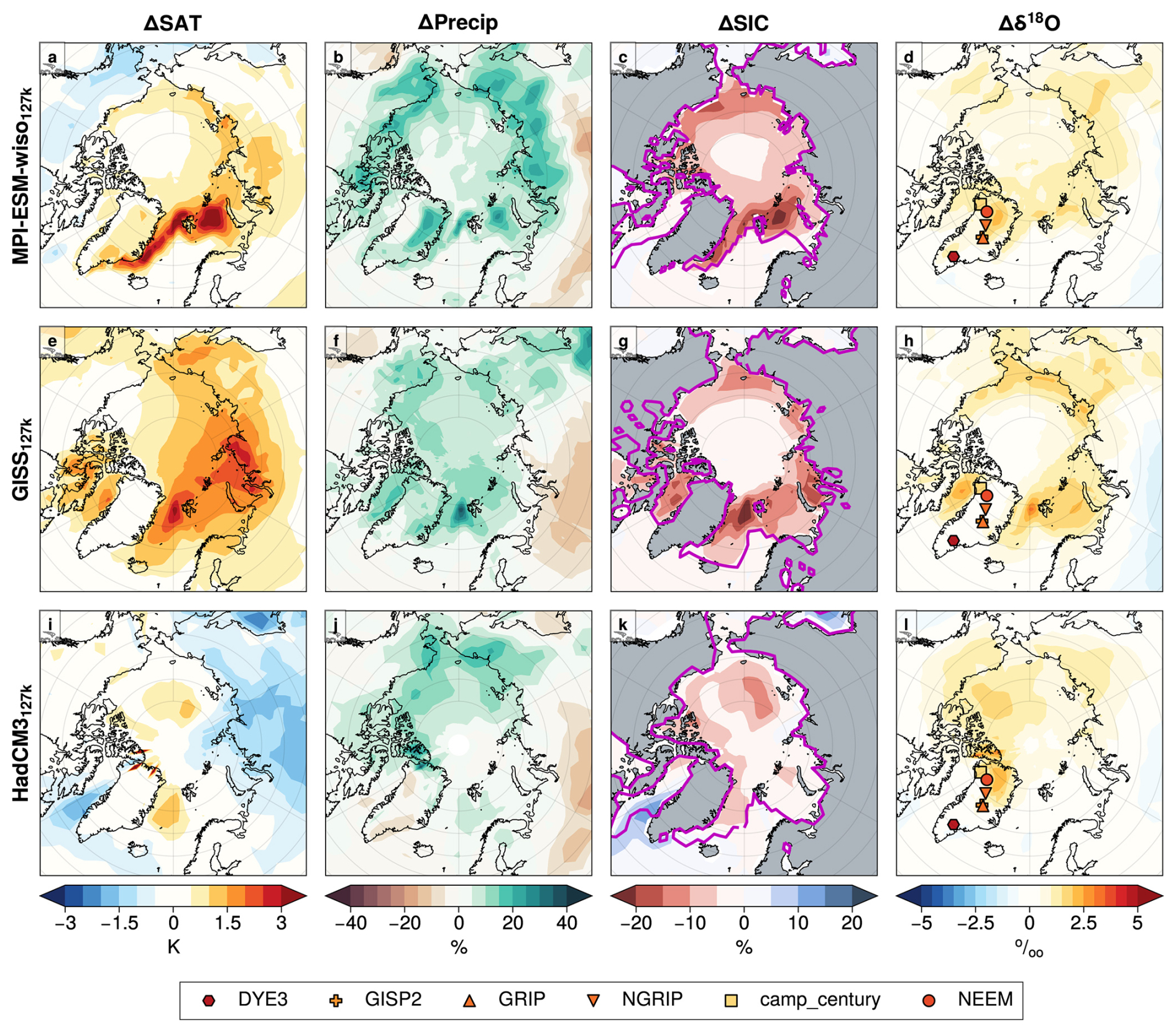
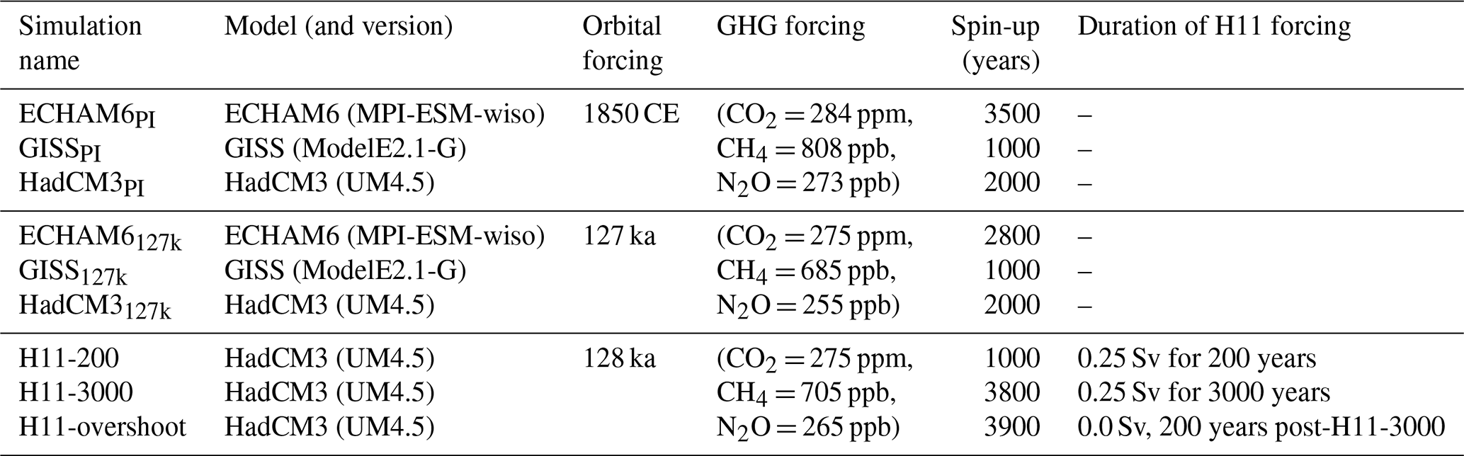
Figure 1 Anomalies in mean annual surface air temperature (ΔSAT), precipitation (ΔPrecip), sea ice concentration (ΔSIA), and δ¹⁸O over the Arctic region for the 127k simulations from the PI. See Table 1 for simulation details. The shaded symbols in the right column show ice core Δδ¹⁸O values as described in Sect. 2.3 and Table A1. Precipitation differences are expressed as percentage deviation from mean PI values. The contours in column 3 indicate the sea ice extent in each PI simulation.

The three 127k simulations show in the Arctic a summer ΔSAT of +1.7 to +2.7 K and a summer ΔSIA reduction of between 35 %–55 % (Table A3). Of the three models, MPI-ESM-wiso and HadCM3 have an absolute 127k summer SIA of 1.7–2.7 mill. km², which is not too far from the expected LIG 127 ka sea ice state (Sime et al., 2023); however, the summer ΔSAT of +1.7 to +1.8 K is roughly half of the observed +3.7 ± 1.5 K warming (Sime et al., 2023; Guarino et al., 2020). Thus, these simulations underestimate both actual 127k summer sea ice loss and associated Arctic summer warming. The 127k simulation that warms the most, the GISS model, has a simulation of both PI and 127k Arctic SIA that is much too large, which makes interpretation of the GISS_127k Arctic changes difficult (cf. Kageyama et al., 2021): effectively whilst there is a huge loss of sea ice from the LIG to the PI, which drives a larger +2.7 K warming of ΔSAT, 6.4 mill. km² remains at 127 kyr, which is more than 5 times the area of the most likely 127 kyr SIA (Sime et al., 2023). This vast extra area of simulated SIA strongly affects SAT, precipitation, and δ¹⁸O, making it more difficult to draw conclusions from this particular GISS simulation. It is easier to draw conclusions from the MPI-ESM-wiso_127k and HadCM3_127k simulation results for the Arctic, whilst bearing in mind that these still show only half the expected summertime ΔSAT. In the case of HadCM3_127k the too-small warming is likely partly due to the PI featuring too little ice, so that summer ΔSIA is relatively small at a 41 % reduction (Table A3). For MPI-ESM-wiso_127k, the PI SIA and ΔSIA is likely a little better, but nevertheless it also shows only half of the expected summer ΔSAT (Table A3).

Figure 2 ΔSAT, ΔPrecip, ΔSIC, and Δδ¹⁸O over the Arctic region for the H11 simulations compared to PI; all columns and rows as for Fig. 1. Note the range of colour bars is wider than in Fig. 1.

Of the H11 HadCM3 simulations (Fig. 2), both H11-200 and H11-3000 show substantial annual-mean growth of sea ice and colder sea surface and air temperatures across the Arctic and North Atlantic: Arctic annual-mean ΔSAT is −0.3, −2.7, and −1.5 K at years 0 (HadCM3_127k), 200 (H11-200), and 3000 (H11-3000) of the H11 meltwater forcing, although due to the orbital forcing Arctic summer ΔSAT is +1.7, +0.8, and +1.2 K at these years (Table A3). However, during the AMOC overshoot, the Arctic becomes much warmer. H11-overshoot shows an Arctic annual-mean ΔSAT of +2.2 K, a summer ΔSAT of +3.0 K, and a practically sea-ice-free Arctic summer SIA of 0.7 mill. km², due to the rapid resumption of the AMOC and advection of warm ocean waters into the Arctic.

Thus, of our six simulations, only H11-overshoot captures the majority of the observed Arctic warming: 81 % of the summer Arctic ΔSAT, a 75 % loss of summer SIA, and an occasionally sea-ice-free Arctic.

3.1.3 Southern Ocean and Antarctic region temperature and sea ice

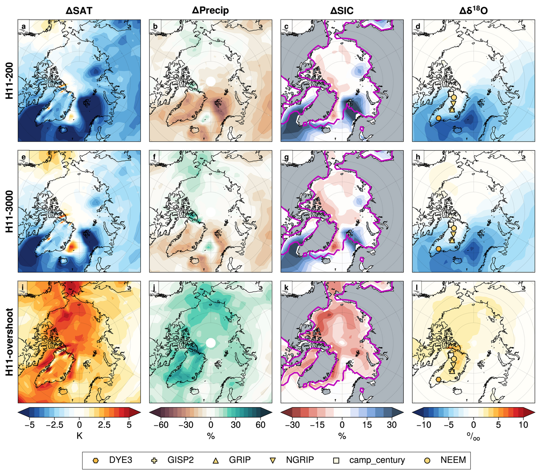
Comparison against the recent synthesis in Gao et al. (2025) allows us to ascertain the percentage of Southern Ocean ΔSST and ΔSIA captured by the simulations (Figs. 3 and 4; Table A4). The three 127k simulations capture no more than 12 % of the 127 ka Southern Ocean warming (Fig. 5). Even MPI-ESM-wiso_127k, which shows a relatively large annual Antarctic reduction of ΔSIA of 23 % and a September sea ice (winter maximum) that is reduced by 63 % (MPI-ESM-wiso generally shows the largest 127k simulation drop in all SIA quantities in both hemispheres), shows little Southern Ocean warming in association with its sea ice loss (Fig. 3a, b; Table A4).

Figure 3 Reconstructed climate anomalies: (a) mean annual ΔSST and ΔSAT, (b) summer ΔSST, and (c) September ΔSIC over the Antarctic and Southern Ocean region for the 127k simulations compared to each PI simulation. Gao et al. (2025) compiled these datasets from Capron et al. (2017), Hoffman et al. (2017), Chandler and Langebroek (2021a), and Chadwick et al. (2021).

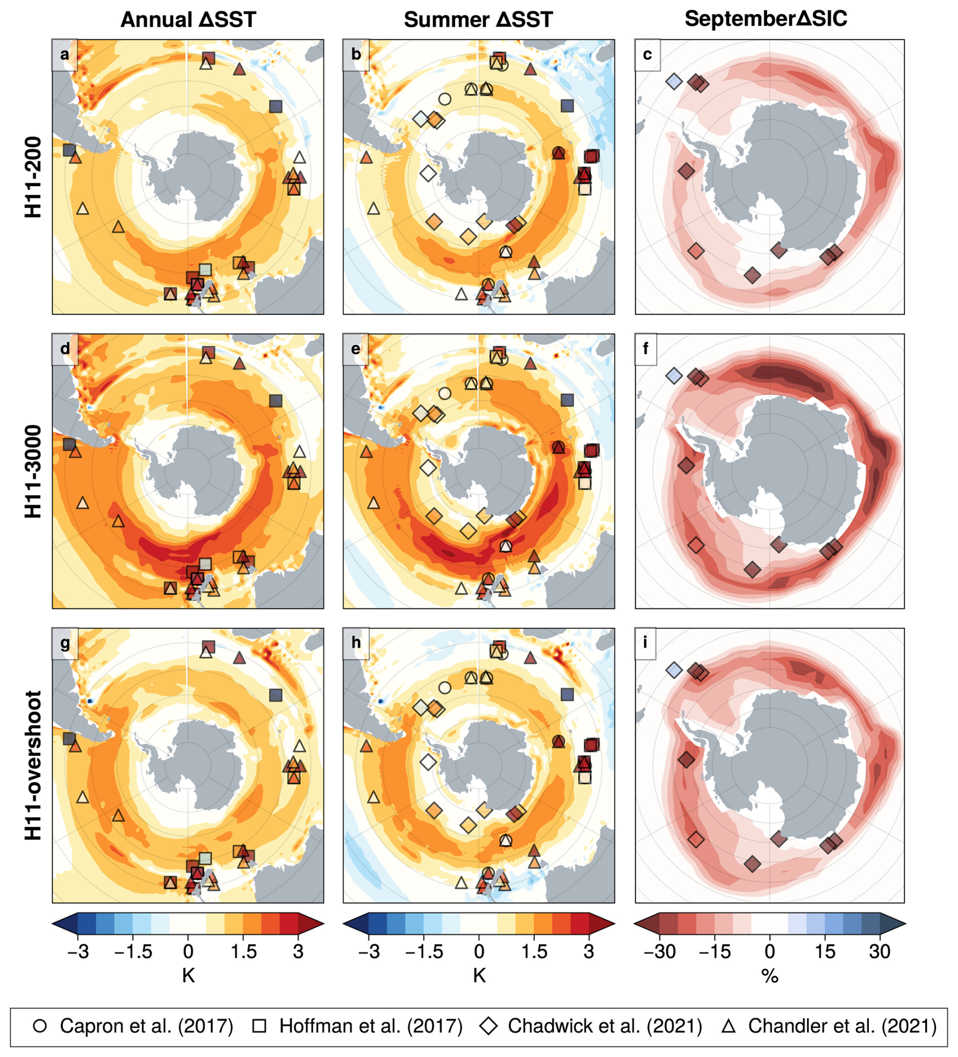
Figure 4 As Fig. 3 but for the H11 simulations compared to the PI simulation.

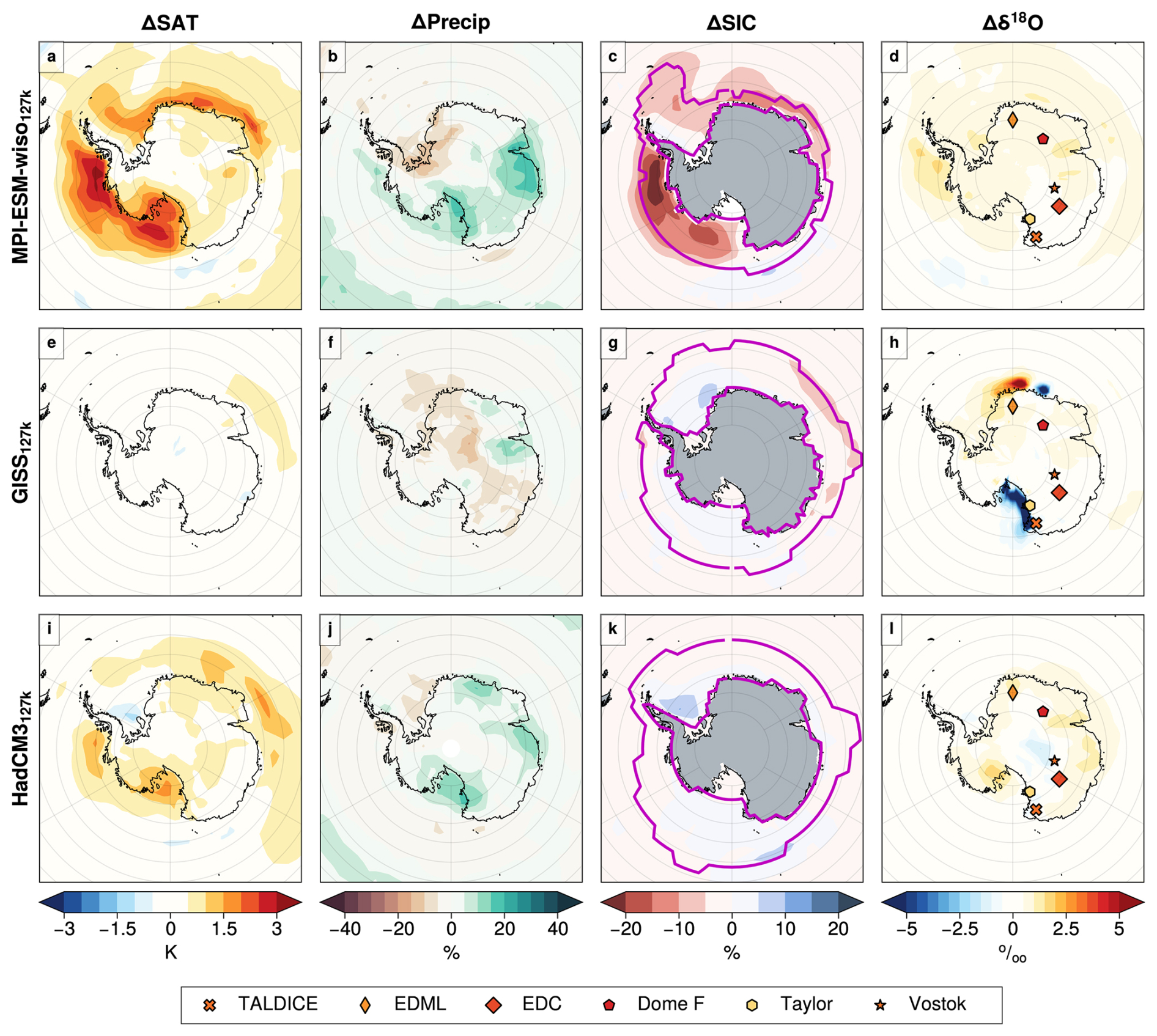
Figure 5 Anomalies in mean annual values: ΔSAT, ΔPrecip, ΔSIC, and Δδ¹⁸O over the Antarctic and Southern Ocean region for the 127k simulations compared to PI; all columns and rows as for Fig. 1.

In contrast, the H11-3000 simulation captures most of the warming and sea ice loss in Gao et al. (2025) (Fig. 4; Table A4). South of 40° S, annual-mean ΔSST rises by 1.3 K, while reconstructed average anomalies range from +2.2 to +2.7 K; summer ΔSST is 1.1 K, close to 1.2–2.2 K reconstructed average anomalies; and September (winter) SIA reduces by 40 %, similar to the reconstructed 40 % reduction of Southern Ocean SIC (Gao et al., 2025). This agreement between the H11-3000 Southern and Global Ocean warming (Sect. 3.1.1) tends to support the idea that it is necessary to take account of the effects of the long H11 meltwater event to allow simulations to capture 127k changes in the Southern Ocean and Antarctic region (Otto-Bliesner et al., 2017; Holloway et al., 2018; Sime et al., 2019a).

Overall, the 127k simulations do not capture the observed Southern Ocean warming and sea ice loss, but the H11-3000 simulation captures between 50 %–100 % of the warming (Table A4), depending on the particular synthesis (Gao et al., 2025) and observation type.

3.2 Changes over the ice sheets: ΔSAT, ΔPrecip, and Δδ¹⁸O

Having looked at how the simulations capture, or not, Global, Arctic, and Southern Ocean ΔSST, ΔGMOT, ΔSAT, and ΔSIA, we now move on to look more closely at the simulation of ΔPrecip and its associated Δδ¹⁸O values over the Greenland and Antarctic ice sheets, with a focus on ice core locations.

3.2.1 Greenland

Most of the 127k simulation ΔSAT, ΔPrecip, and Δδ¹⁸O changes are strongly associated with sea ice changes, including ΔSIA but also the initial (PI) sea ice state, particularly the summertime changes (Sect. 3.1.2 and Fig. 1).

GISS_127k has more than 6 mill. km² of Arctic SIA left in the summer, meaning there is little open water or associated opportunity for proximal sea evaporation in summer. It therefore shows very little change in ΔSAT, ΔPrecip, and Δδ¹⁸O over Greenland (Fig. 1), and its Greenland core-mean Δδ¹⁸O value is 0.0 ‰. In contrast, because HadCM3_127k and MPI-ESM-wiso_127k have summertime 127k SIAs of 1.7 and 2.7 mill. km², their Δδ¹⁸O are enriched by +0.6 ‰ and +1 ‰, respectively. This is still considerably smaller than the observed core-mean Δδ¹⁸O of +3.2 ‰ (Table A1). Thus, the mean Arctic summertime ΔSAT is about half of the observed value, but the Greenland core-mean Δδ¹⁸O values are only one-quarter to one-third of the observational estimates (Domingo et al., 2020; Sime et al., 2023).

There are also variations across Greenland in ΔPrecip and Δδ¹⁸O between the 127k simulations. For example, HadCM3_127k tends to be drier across southern Greenland, but the isotopic response over northern Greenland is much stronger, even when the precipitation increase there is weaker compared to MPI-ESM-wiso and GISS. This could be indicative of a more detailed source- and transport-related response in δ¹⁸O. Although outside the scope of this paper, further water tracer simulations might be useful to diagnose these (e.g. Gao et al., 2024a).

For the H11-200 and H11-3000 simulations Δδ¹⁸O is depleted over Greenland and the wider northern Atlantic sector, commensurate with the mean-annual SIA increase and cooling (Sect. 3.1.2 and Fig. 8). However, the warm Arctic and summer sea-ice-free Arctic of H11-overshoot leads to strongly enhanced precipitation and reduced sea ice, all of which contributes to the very substantial H11-overshoot increase over the Greenland core-mean Δδ¹⁸O of 2.8 ‰, compared to a Greenland core-mean Δδ¹⁸O of 3.2 ‰: i.e. H11-overshoot captures 81–87 % of both summer Arctic ΔSAT and Greenland core-mean Δδ¹⁸O.

3.2.2 Antarctica

Section 3.1.3 indicates that the 127k simulations do not capture much of the observed Southern Ocean region warming. So, in turn, the Antarctic ΔSAT, ΔPrecip, and Δδ¹⁸O 127k simulation changes are also very small and not consistently in the correct direction relative to Antarctic core site 127 ka measurements (Fig. 5; Table A1): core-mean Δδ¹⁸O results are +0.0 ‰, −1.0 ‰, and +0.3 ‰ for HadCM3_127k, GISS_127k, and MPI-ESM-wiso_127k, respectively. This is compared with an observed core-mean Δδ¹⁸O value of +3.3 ‰. This is somewhat like the Greenland 127k results, which also indicate that the mismatches with observed ice core Δδ¹⁸O seem mostly driven by simulation of sea ice and SST changes, or lack thereof.

Within Antarctica, of the three 127k simulations, the MPI-ESM-wiso_127k features the strongest Antarctic surface warming, including a strong warming around the west side of the Antarctic Peninsula and over other coastal regions. This likely is because it does show some 127k simulation Antarctic sea ice loss. The sea ice loss also leads to rather uniform δ¹⁸O enrichment across the Antarctic and surrounding ocean. GISS_127k and HadCM3_127k show different patterns of Δδ¹⁸O across Antarctica. HadCM3 simulates slight enrichment of δ¹⁸O towards inland Antarctic, while GISS_127k simulates strong enrichment around the Ross Sea sector. Unlike MPI-ESM-wiso_127k, GISS_127k and HadCM3_127k do not show significant sea ice reduction, although HadCM3_127k does simulate surface warming over Antarctic and coastal oceans but not as strong as MPI-ESM-wiso_127k. GISS_127k does not show much change in ΔSAT. Both MPI-ESM-wiso_127k and HadCM3_127k are wetter (larger ΔPrecip) over the Ross Sea sector. MPI-ESM-wiso_127k is drier across the Weddell Sea to Dronning Maud Land, while GISS_127k is drier inland, with the only exception over the East Antarctic from around 60–100° E. It is difficult to know what, if anything, to draw from these multi-model variations.

Figure 6 Anomalies in mean annual values: ΔSAT, ΔPrecip, ΔSIC, and Δδ¹⁸O over the Antarctic and Southern Ocean region for the H11 simulations; all columns and rows as for Fig. 1. Note the range of colour bars is wider than in Fig. 5, except for δ¹⁸O.

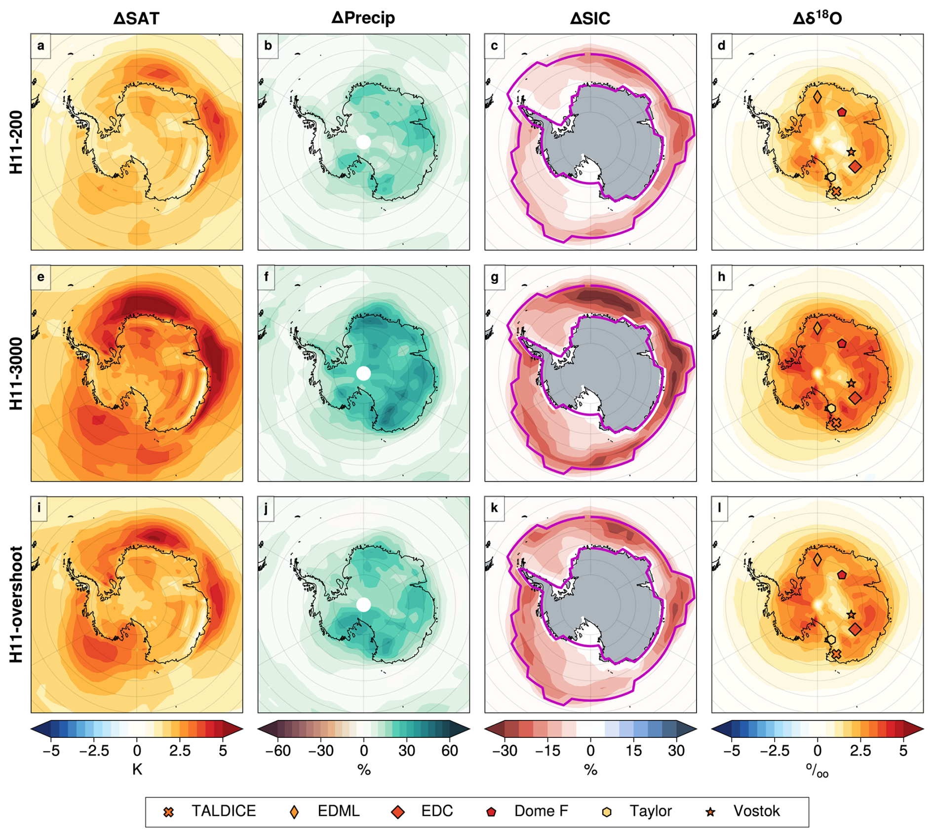
Over Antarctica the H11 simulations show relatively uniform ΔSAT, ΔPrecip, and Δδ¹⁸O (Fig. 6). The H11 Antarctic core-mean values for ΔSAT are +0.5, +2.0, +3.0, and +2.4 K at 0, 200, and 3000 years and for the overshoot. Core-mean Δδ¹⁸O values of +0.0 ‰, +1.9 ‰, +3.1 ‰, and +2.3 ‰ follow a similar pattern to the temperature changes (Table A1; Fig. 6). These simulated values compare to the observed core-mean Δδ¹⁸O value of 3.3 ‰. This means that the H11-3000 simulation captures 94 % of the observed Antarctic core-mean Δδ¹⁸O. This is commensurate with the previous sections which also show that the longer H11-3000 simulation also captures 50 %–100 % of the Southern Ocean warming and sea ice loss.

3.3 The impact of changes in seasonality on Δδ¹⁸O

Decomposition of the impact of changes in seasonality on Δδ¹⁸O can be useful to better understand drivers of Δδ¹⁸O. See Sect. 2.2.2 for a description of the breakdown of Δδ¹⁸O into the two terms ΔPrecip_seasonal (precipitation seasonality changes) and Δδ¹⁸O_seasonal (δ¹⁸O seasonality, or source effect, changes) that are used here.

3.3.1 Arctic

For the 127k simulations, precipitation-source-related (Δδ¹⁸O_seasonal) changes in the Arctic, particularly for MPI-ESM-wiso_127k and GISS_127k, contribute strongly to the enrichment in δ¹⁸O in regions of large sea ice loss; where there is increased exposure of the ocean surface, there will be more (local) evaporation (Fig. 7, first and third column). Given the large summer losses of Arctic sea ice, we would also expect to see an increase in summer precipitation for some simulations. Likely due to their small Arctic SIAs, HadCM3_127k and MPI-ESM-wiso_127k do show the largest contribution from seasonal shift of precipitation (increase in warm season precipitation, ΔPrecip_seasonal) to Δδ¹⁸O over the Arctic. Indeed for HadCM3_127k most of the increase in Δδ¹⁸O is associated with these ΔPrecip_seasonal precipitation seasonality changes. For MPI-ESM-wiso, the contributions of ΔPrecip_seasonal and Δδ¹⁸O_seasonal are more similar. Figures 1 and A3–A7 depict how ΔPrecip_seasonal changes in these models depend largely on the loss of summertime high Arctic sea ice, which drives an increase in (local) warm season precipitation (Fig. 7, middle column).

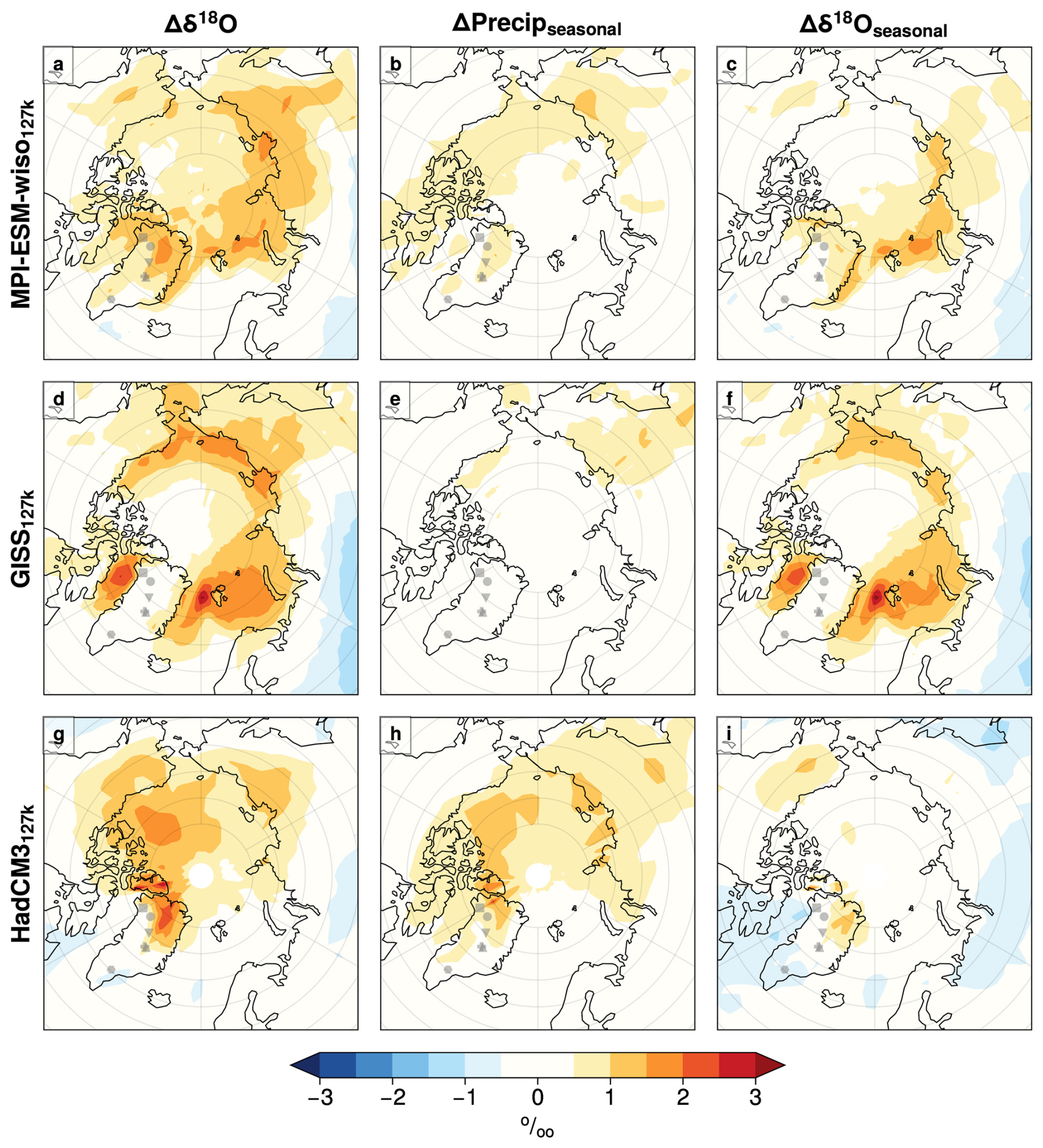
Figure 7 The impact of seasonality change on Δδ¹⁸O: decomposition of Δδ¹⁸O values into contribution from seasonal variability in precipitation (ΔPrecip_seasonal) and source variability (Δδ¹⁸O_seasonal) in the Arctic for the 127k simulations. See Sect. 2.2.2 for full details.

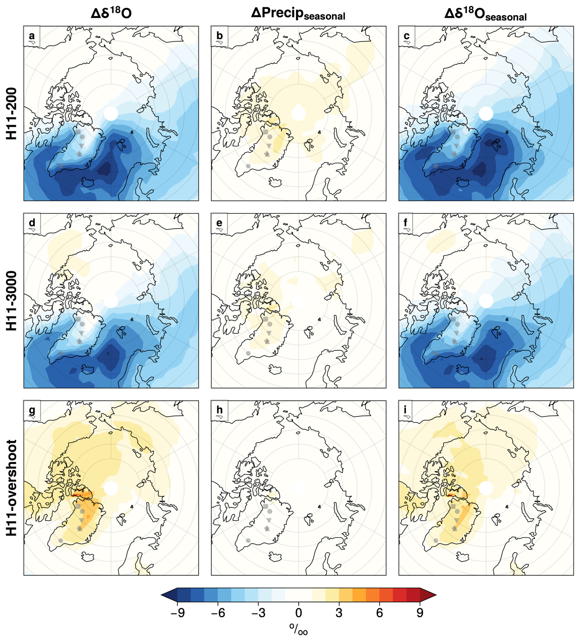
Figure 8 The impact of seasonality change on Δδ¹⁸O: decomposition of Δδ¹⁸O values into contribution from seasonal variability in precipitation (ΔPrecip_seasonal) and source variability (Δδ¹⁸O_seasonal). Differences between the PI and H11 simulations; all columns and rows as for Fig. 7.

There is also some relationship between the two separate seasonality terms: the increased Δδ¹⁸O_seasonal term does tend to contribute to the enrichment in δ¹⁸O where ΔPrecip also increases (Fig. 1), indicating that rainout and distance to source effects on δ¹⁸O are sometimes closely related. As would be expected, where ΔPrecip decreases Δδ¹⁸O_seasonal also tends to decrease.

For the H11 simulations, although HadCM3_127k and H11-overshoot both show a warmer Arctic, the decomposition of Δδ¹⁸O for each simulation shows distinctly different behaviour (Fig. 10). As above, whilst for HadCM3_127k most of the increase in Δδ¹⁸O is associated with ΔPrecip_seasonal, this is completely reversed for H11-overshoot, with almost all of the increase driven by Δδ¹⁸O_seasonal rather than ΔPrecip_seasonal. This is because there is a large annual-mean, including wintertime, loss of sea ice in H11-overshoot, driven by the increased AMOC and global ocean temperature (rather than purely the orbital 127k spring–summer losses), leading to much more wintertime, and closer-sourced wintertime, precipitation over Greenland.

3.3.2 Antarctica

For the mainly orbitally driven 127k simulations in Antarctica, precipitation seasonality changes (ΔPrecip_seasonal) contribute to the depletion in δ¹⁸O over Antarctica (Fig. 9, middle column). For simulations where overall precipitation is increasing/not changing, including HadCM3_127k and for the Ross Sea/East Antarctic sector in MPI-ESM-wiso_127k, this can be explained by relative increase in precipitation that falls during colder seasons during the 127k simulations relative to the PI, leading to reduced δ¹⁸O. However, opposing this, sea ice retreat and shorter source-to-site vapour transport pathways can raise δ¹⁸O values (Fig. 9, right column). Together these two terms (the seasonality of precipitation and seasonality of δ¹⁸O changes) can therefore lead to rather small, sometimes near-zero simulated Δδ¹⁸O across Antarctica between the LIG and PI for the 127k simulations (Fig. 9).

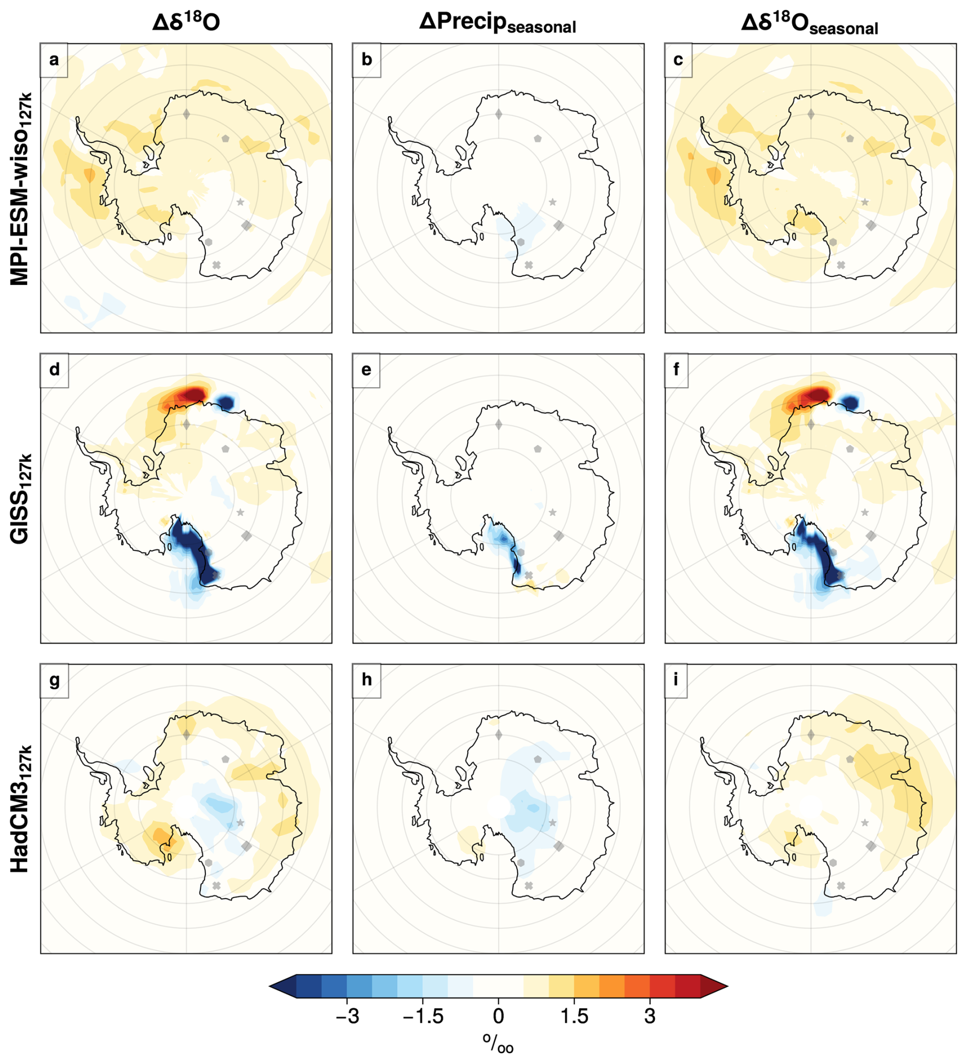
Figure 9 The impact of seasonality change on Δδ¹⁸O: decomposition of Δδ¹⁸O values into contribution from seasonal variability in precipitation (ΔPrecip_seasonal) and source variability (Δδ¹⁸O_seasonal). Differences between the PI and 127k simulations for the Antarctic region; all columns and rows as for Fig. 7.

The GISS_127k simulation has a very unique pattern of δ¹⁸O change in the Antarctic, with extreme low values over the Ross Sea sector and a very local pattern of low and high values in the East Antarctic coastline around Dronning Maud Land. The surface temperature increase and sea ice reduction in the Antarctic is minimal in this model compared to the other two, and the precipitation changes indicate a change towards a drier 127k simulated Antarctic. We are unsure if the Antarctic δ¹⁸O extremes indicate an issue with this particular simulation. We do not consider these extreme values further here.

The H11 simulations all show larger increases in δ¹⁸O compared to the 127k simulations, in response to the increased SST/SAT and reduced sea ice. Here the negative precipitation seasonality changes, ΔPrecip_seasonal, are dwarfed by the impact of the Δδ¹⁸O_seasonal terms. This means that sea ice retreat and shorter source-to-site vapour transport pathways, particularly in the colder and shoulder seasons, act to strongly raise δ¹⁸O values (Fig. 10, right column). For H11-overshoot, the Antarctic and Southern Ocean temperature and sea ice do not reverse to their pre-H11 state (i.e. HadCM3_127k state) after 200 years of no meltwater: once the AMOC recovered to the initial strength (Fig. A2) elevated global and polar temperature take time to cool; thus, Antarctic δ¹⁸O values remain high more than 200 years after the H11 hosing has stopped.

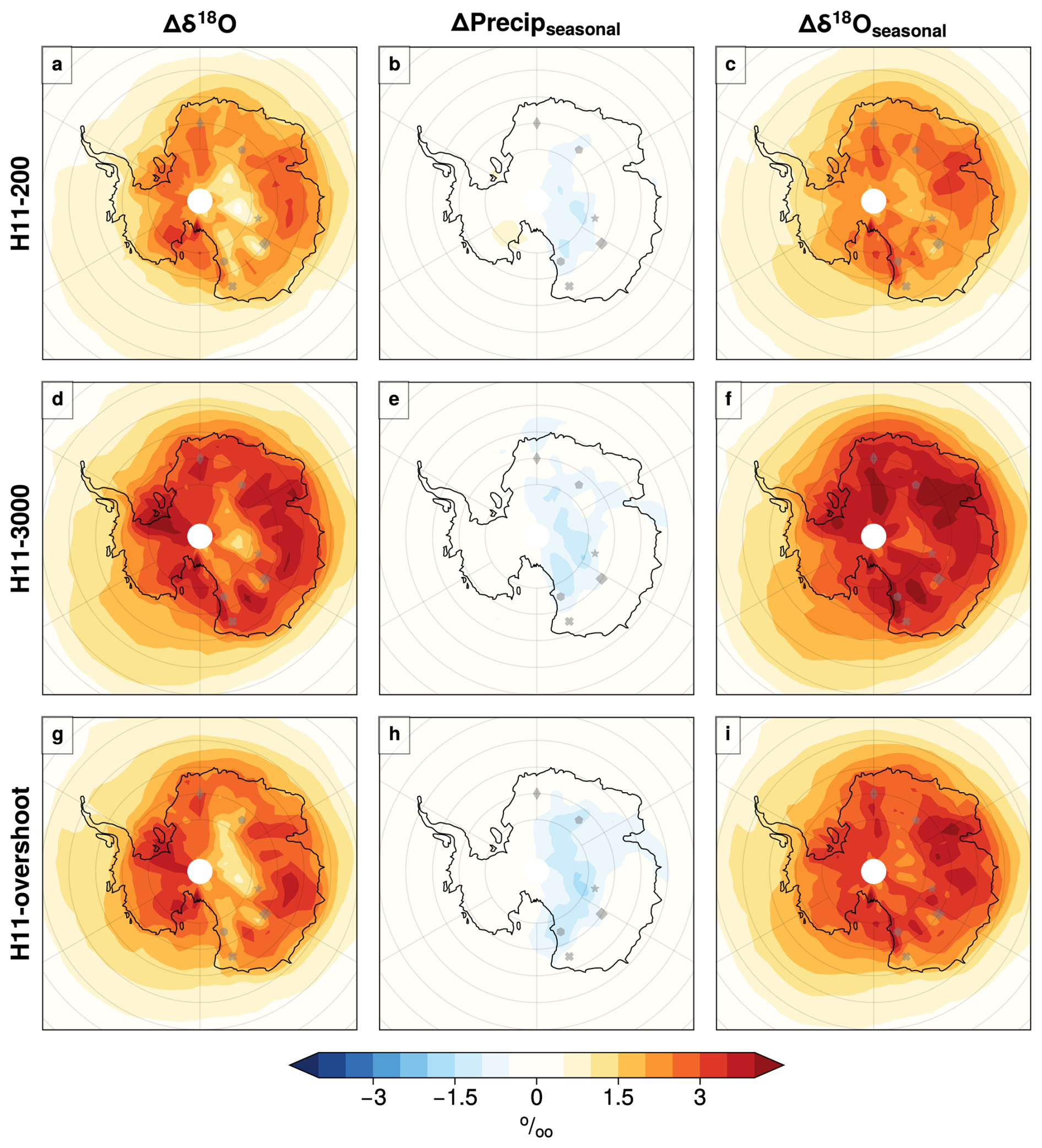
Figure 10 The impact of seasonality change on Δδ¹⁸O: decomposition of Δδ¹⁸O values into contribution from seasonal variability in precipitation (ΔPrecip_seasonal) and source variability (Δδ¹⁸O_seasonal). Differences between the PI and H11 simulations for the Antarctic region; all columns and rows as for Fig. 7.

In Antarctica every ΔPrecip_seasonal result – for each of the six simulations – is small, with some negative regions, i.e. some regions of more colder-season precipitation. Δδ¹⁸O_seasonal is always larger and tends to dominate Antarctic Δδ¹⁸O for each simulation, mostly due to sea-ice-related changes (Figs. 5, 9, and 10, first and last columns).

3.4 Implications for the interpretation of ΔSAT from Δδ¹⁸O in ice cores

The interpretation of Δδ¹⁸O values in polar ice cores as a proxy for past temperatures is a critical component of palaeoclimate reconstructions. Past LIG temperature estimates derived from δ¹⁸O values at key Greenland and Antarctic sites, such as NEEM, Dome C, Vostok, and Dome F, have generally been obtained by converting Δδ¹⁸O to SAT using palaeothermometer gradients. For instance in Greenland at the NEEM ice core, NEEM community members (2013) converted Δδ¹⁸O to SAT using a palaeothermometer gradient of 2.1±0.5 K ‰⁻¹, which was based on data from Vinther et al. (2009). This means that the NEEM Δδ¹⁸O value of +3.6 ‰ implies that, without taking account of any ice flow influences on site temperature, peak LIG surface temperatures were $+\mathrm{7.5}\pm \mathrm{1.8}$ K warmer than the PI.

For Antarctica, Jouzel et al. (2007) applied a gradient of 1.43 K ‰⁻¹; Petit et al. (1999) and Masson-Delmotte et al. (2006) used a gradient of 1.33 K ‰⁻¹; and Sime et al. (2009), based on isotope-enabled model simulations focussed on 2100, proposed a palaeothermometer gradient for the East Antarctic Dome C (EDC) core around 1.7 K ‰⁻¹ and suggested that regional and temporal variability in the palaeothermometer gradient might be more significant than previously thought. The simulations presented here enable examination of the consistency of the relationships between ΔSAT and Δδ¹⁸O across all the LIG_127k and LIG_H11 simulations.

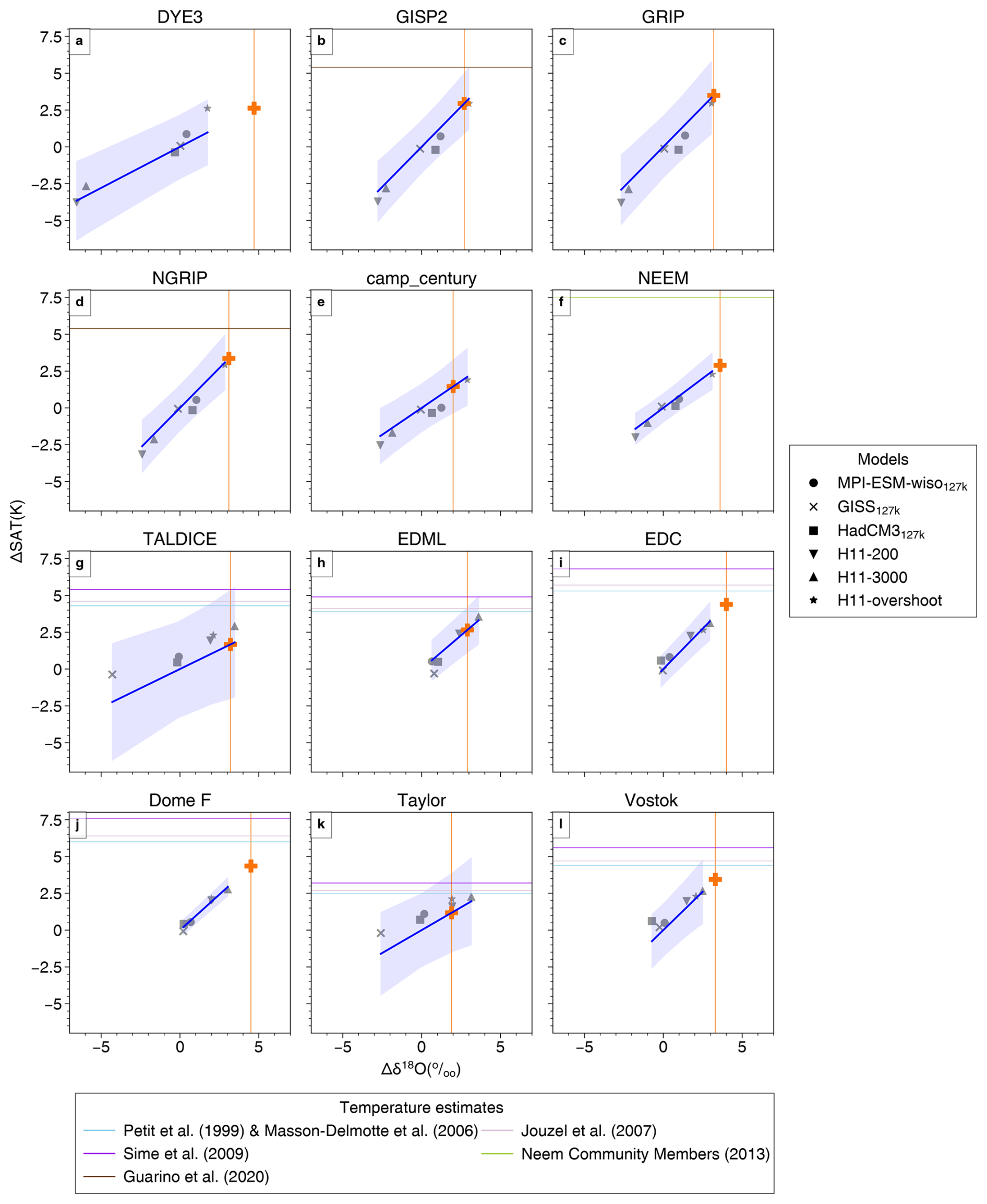
Figure 11 Δδ¹⁸O versus ΔSAT for different simulations for each ice core site. Fits are calculated as described in Sect. 2.2.3. Shaded bands show the 95 % uncertainty envelope. Vertical orange lines indicate the ice core Δδ¹⁸O values (Table A1). Horizontal lines indicates temperature estimates for each ice core location from previous studies, whilst orange crosses indicates our estimated central ΔSAT values obtained from the simulation fits, i.e. projected using the fitted modelled Δδ¹⁸O–ΔSAT (blue line) relationships.

Standard errors and uncertainties for gradients for H11 simulations are smaller than where LIG_127k simulation results are used alone (Tables 2 and A5). This is primarily because the H11 simulations show larger ΔSAT and Δδ¹⁸O values than the 127k simulations and so exert a stronger influence on the gradient of the regression lines fitted to ΔSAT and Δδ¹⁸O (Fig. 11 and Table A1). Given Sect. 3.1–3.3 show that these H11 simulations do a better job of capturing peak LIG warmth and sea ice changes at both poles, compared to the 127k simulations, this larger influence seems reasonable. We also find that if regression fits are applied to LIG_127k simulation results alone, without including the H11 simulations, gradients are not inconsistent, if very uncertain (Table A5). This suggests that the underlying physics driving the δ¹⁸O–SAT relationship is consistent across different LIG climate states, even if the 127k simulations alone are insufficient to derive accurate gradients. Here we therefore use all the simulation results to derive LIG temperature estimates from Δδ¹⁸O values at Greenland and at Antarctic core sites.

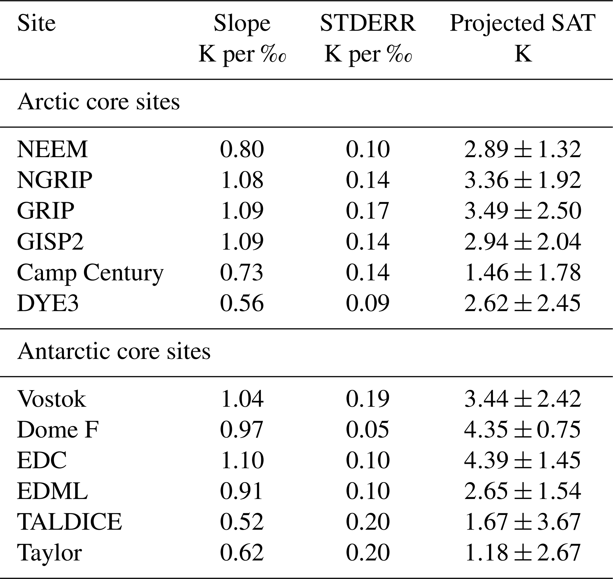
Table 2 Relationships between SAT and δ¹⁸O, calculated using all model simulations for each site. Fits use Δδ¹⁸O as the dependent variable and ΔSAT as the independent variable to enable projection of ΔSAT from Δδ¹⁸O. See also Sect. 2.2.3. The projected ΔSAT values are shown with 95 % confidence intervals and are based on the ice core Δδ¹⁸O values in Table A1. STDERR: standard error.

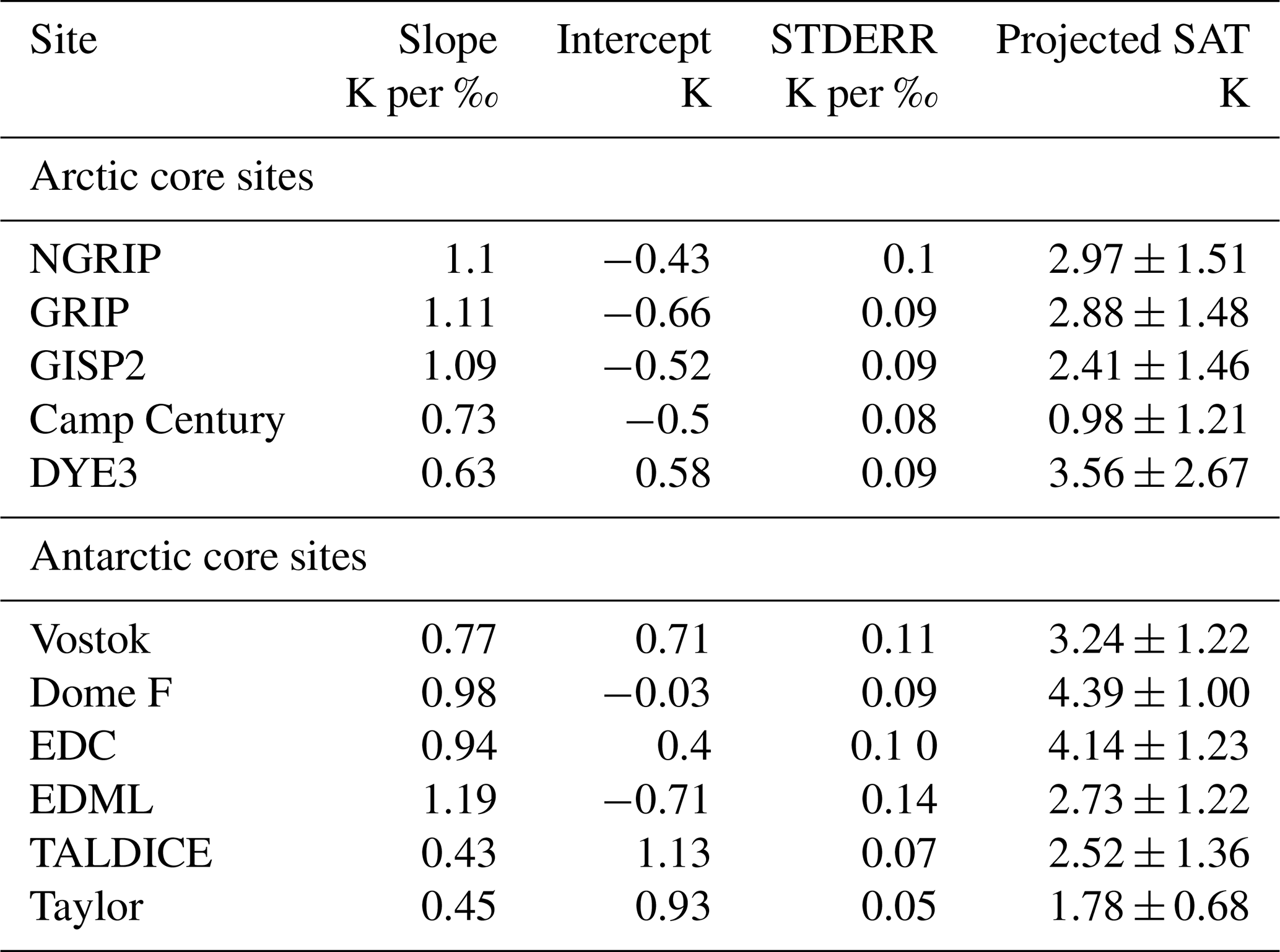
The results in this section use primarily one-part fits (Sect. 2.2.3). These assume that ΔSAT and Δδ¹⁸O are co-dependent and that they always tend to change together. However, note that using a two-part fit, i.e. a regression line which permits a non-zero intercept (Table A7 and Fig. A9), gives results which agree, within uncertainties, with these one-part fits. Thus, this choice is not significant to our findings. Section 2.2.3 explains fit methods and the calculation of uncertainties.

3.4.1 Greenland – NEEM

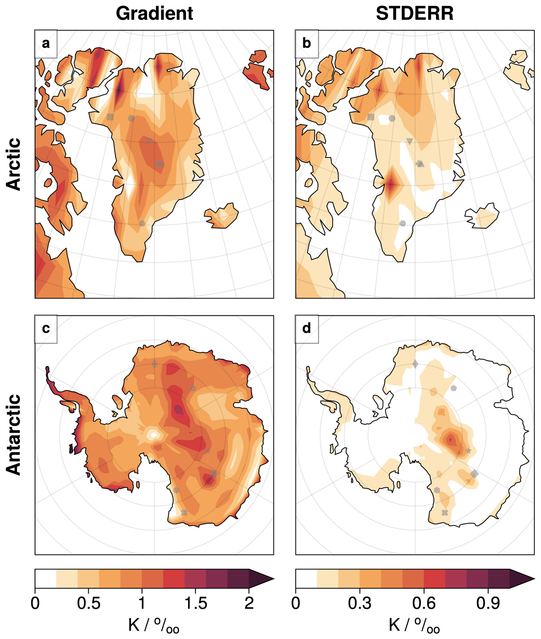
The interpretation of LIG temperature from Δδ¹⁸O values measured in Greenland ice has only been attempted for the NEEM ice core (NEEM community members, 2013). This is likely because, as outlined in Sect. 2.3, the dating of LIG ice for most Greenland ice cores is difficult due to stratigraphic disturbances in the ice of this age. Interestingly, the simulations used here show a substantially lower gradient of 0.8 K ‰⁻¹ at NEEM – less than half of that used in NEEM community members (2013). Other ice core sites in central Greenland have a slightly higher gradient of around 1.1 K ‰⁻¹ at NGRIP, GRIP, and GISP2. Based on the Sect. 2.3 value (in Table A1), these suggest that, without taking account of any site elevation or other ice flow effects, there was a PI to LIG warming of $+\mathrm{2.89}\pm \mathrm{1.32}$ K at NEEM and $+\mathrm{3.49}\pm \mathrm{2.5}$ K at GRIP. Table 2 and Figs. 11 and 12a show that the gradients across Greenland are relatively uniform, but with a tendency towards higher K ‰⁻¹ gradients inland compared to the coast.

Figure 12 Maps of Δδ¹⁸O versus ΔSAT gradient and associated standard error, calculated at each grid point using all simulations. The fitting procedure is described in Sect. 2.2.3, and ice core sites are shown, for example, in Fig. 11.

3.4.2 Antarctica

The relationship between Δδ¹⁸O and ΔSAT shows considerable variation across Antarctica (Fig. 12, Antarctic row), particularly between the high East Antarctic plateau (like Vostok, Dome F, and EDC) and more coastal sites (like TALDICE and Taylor): gradients tend to be higher across the plateau (Table 2). This same spatial pattern in gradients is also reflected in relationships between Δδ¹⁸O and other quantities like ΔSIA (Fig. A8). These differences underscore that it may be necessary to use site and time-specific palaeothermometer gradients rather than applying a uniform and constant gradient across all Antarctic locations and periods. Like Greenland above, central Antarctica has higher K ‰⁻¹ gradients compared to the coastal regions.

The gradients derived from these simulations at the Vostok, Dome F, and EDC ice core sites range from 0.9 K ‰⁻¹ to 1.1 K ‰⁻¹. These are a little lower than the canonical values often used in previous studies (1.3 K ‰⁻¹–1.4 K ‰⁻¹) (Petit et al., 1999; Masson-Delmotte et al., 2006; Buizert et al., 2021). For example, Werner et al. (2018) set up eight atmospheric model simulations using ECHAM5-wiso with different Last Glacial Maximum (LGM) ice sheet reconstructions to investigate the temporal and spatial relationships between δ¹⁸O and SAT across Antarctica. They found that, whilst these LGM to PI relationships differed across Antarctic regions, they tended to be close to a commonly identified relationship of around 1.25 K ‰⁻¹. That said, Cauquoin et al. (2023) note that ECHAM5-wiso tends to significantly overestimate isotope changes in Antarctica compared to more recent ECHAM6-wiso simulations, even under identical boundary conditions. Thus, some questions about LGM to PI Δδ¹⁸O and ΔSAT relationships remain. Indeed it is possible that as yet we do not have reliable multi-model isotopically enabled LGM simulations.

Applying these LIG multi-model simulation-derived gradients to the Δδ¹⁸O ice core values in Table A1 yields inferred past peak interglacial surface air temperature increases. These are 4.35±0.75 K for Dome F, 3.44±2.42 K for Vostok, and 4.39±1.45 K for EDC, on the high East Antarctic plateau. For the more coastal sites of TALDICE and Taylor, more modest increases of 1.67±3.67 and 1.18±2.67 are inferred. However, if two-part fits are allowed for these coast sites – i.e. SAT can rise between PI and peak-LIG – Table A7 shows larger past peak interglacial surface air temperature increases of 2.52±1.36 and 1.78±0.66, which are somewhat closer to the inland core site rises.

In summary, these results together suggest a more modest PI to peak-LIG temperature increase across Antarctica compared to earlier estimates. We attribute this difference primarily to the substantially improved representation of LIG sea surface conditions around Antarctica, particularly for sea ice, which enables a better representation of the key ΔSAT, ΔPrecip, and Δδ¹⁸O changes.

4 Conclusions

The Last Interglacial (LIG), from about 130 000 to 115 000 years ago, is one of the warmest periods in recent geological history (Hoffman et al., 2017; Fischer et al., 2018), with warming that may be similar to predictions for the end of this century (IPCC, 2021). However, reconstructing peak LIG temperatures around 127 ka from ice cores can be challenging due to unknowns about the relationship between water isotopes (δ¹⁸O) and temperature.

This study used three isotope-enabled climate models – HadCM3, MPI-ESM-wiso, and GISS ModelE-R – in the first multi-model analysis of the LIG. Standard 127k simulations, following the PMIP4 (orbital and greenhouse gases) protocol (Otto-Bliesner et al., 2017), were run for each model. These simulations were complemented with a long 3000-year LIG H11 simulation run using HadCM3.

The 127k simulations tend to show slight global cooling, but the H11 simulations, especially the extended H11-3000 and H11-overshoot simulations, capture significant warming trends that are consistent with the LIG observations of peak warmth (Fischer et al., 2018; Shackleton et al., 2020). In particular, the H11-overshoot simulation appears to accurately represent peak LIG Arctic conditions, replicating 81 % of the peak summer temperature increase, reducing summer sea ice by 75 %, and showing periods of nearly ice-free Arctic summers. This simulation also matched the observed peak LIG changes in Greenland ice core δ¹⁸O, with a 2.8 ‰ increase, close to the observed 3.2 ‰. We note that some parts of the remaining 0.4 ‰ missing part of the simulated isotope signal could be due to vegetation or ice sheet feedbacks which are not included in these simulations (Claussen et al., 2006; Schurgers et al., 2007; Nikolova et al., 2013; Otto-Bliesner et al., 2006). Further, we note that the lack of a sea-ice-free Arctic in summer in the 127k simulations may reflect deficiencies in the sea ice submodel (Guarino et al., 2020; Diamond et al., 2023; Sime et al., 2023). In future, Arctic and Greenland δ¹⁸O results in models with alternative sea ice submodels should be explored.

In Antarctica, the H11-3000 simulation successfully captured 50 %–100 % of the peak LIG Southern Ocean warming and sea ice loss and 94 % of the observed increases in ice core Δδ¹⁸O. This highlights both the importance of including prolonged meltwater events in climate models to accurately capture peak LIG conditions and the necessity of a good polar climate to simulate ΔSAT, ΔPrecip, and Δδ¹⁸O over the ice sheets.

Our H11 simulation is highly idealized (Holloway et al., 2018; Gao et al., 2025), and so we emphasize it cannot be tied to particular time points within the LIG. On timing, however, recent results of Shackleton et al. (2020) suggest a LIG peak in GMOT around 129 ka. Our simulation results suggest this should be coincident with the end of the H11 – NH deglaciation – meltwater event. This appears to be in agreement with Stoll et al. (2022), who show that whilst the bulk of the Northern Hemisphere deglaciation occurred between 134–130 ka, global sea level continued to increase due to meltwater until 129 ka or a little after. Additionally, given H11-3000 simulates our warmest Southern Ocean and Antarctic state and within 100 years H11-overshoot simulates our warmest Arctic and Greenland state, peak SST and SAT temperatures, as well as a minimum in SIA, may have occurred within a rather short time span for both Greenland and Antarctica. Timescales for deeper ocean changes are, however, slower and will have a different pattern of evolution. Further work should examine how short-lived the H11-overshoot is for the Arctic, alongside its interaction with the period of very high early-summer insolation that is also centred around 127 ka.

The use of Δδ¹⁸O values in polar ice cores as a temperature proxy is key to reconstructing past climates. Temperature estimates from δ¹⁸O at sites like NEEM, Dome C, Vostok, and Dome F during the Last Interglacial (LIG) rely on converting Δδ¹⁸O into ΔSAT using palaeothermometer gradients. Our simulations suggest a gradient of 0.8 K ‰⁻¹ at NEEM, which is less than half that used by NEEM community members (2013), with slightly higher values, around 1.1 K ‰⁻¹, at central Greenland sites such as NGRIP, GRIP, and GISP2. Interestingly, these revised values are quite close to those from Lee et al. (2008), who find spatial relationships of about 0.8 K ‰⁻¹ between annual-mean temperature at the top of the inversion layer and annual-mean δ¹⁸O in precipitation (Liu et al., 2023). Further work is needed to understand the role of inversion layers in shaping these relationships during the LIG. In future studies, it may also be valuable to examine local-to-regional influences, such as changes in local boundary layer conditions (Krinner et al., 1997; Noone and Simmonds, 2002) and continental vapour recycling impacts (Werner et al., 2001; Werner and Heimann, 2002; Sjolte et al., 2014), alongside larger-scale effects such as distal source property and pathway changes (Boyle, 1997; Kindler et al., 2014; Guan et al., 2016). Isotope-enabled models and associated water tracking tools are particularly helpful for ensuring that these factors are included when examining relationships between Δδ¹⁸O and ΔSAT (Jouzel et al., 1997; Gao et al., 2024a; McLaren et al., 2025).

Use of these Δδ¹⁸O–ΔSAT relationships from the new LIG simulations suggests PI-to-LIG warming values of $+\mathrm{2.89}\pm \mathrm{1.32}$ K at NEEM and $+\mathrm{3.49}\pm \mathrm{2.5}$ K at GRIP. These estimates do not account for site elevation or ice flow effects and are substantially lower than previously suggested warming values. For Antarctica, our simulated δ¹⁸O–temperature gradients at sites including Dome C, Dome F, and Vostok range from 0.9 K ‰⁻¹ to 1.1 K ‰⁻¹, slightly lower than previously published values of 1.3 K ‰⁻¹–1.4 K ‰⁻¹ (Petit et al., 1999; Masson-Delmotte et al., 2006). Applying these updated gradients, the estimated peak temperature increases between the PI and LIG are 4.39±1.45 K for Dome C, 4.35±0.75 K for Dome F, and 3.44±2.42 K for Vostok. These findings suggest a more modest temperature rise during the LIG for both Greenland and Antarctica than previously thought. This revision is largely due to improved representation of polar sea ice changes in the new extended H11 simulations.

However, it is important to note that these revised temperature estimates do not incorporate any corrections for ice core site-elevation- or other ice-flow-related impacts on site temperatures. Future efforts should focus on better characterizing LIG Antarctic and Greenland ice sheet changes, which influence both δ¹⁸O and temperature (Holloway et al., 2016; Werner et al., 2018; Domingo et al., 2020; Goursaud et al., 2021; Zou et al., 2025), as well as on the role of potential vegetation feedbacks (Claussen et al., 2006; Schurgers et al., 2007; Nikolova et al., 2013; Otto-Bliesner et al., 2006). In addition, a re-examination of the nature and timing of peak polar ice sheet warmth and its coincidence between Antarctica and Greenland is warranted. Finally, the application of newly developed water tracking tools in climate models may provide further insight into the drivers of Δδ¹⁸O–ΔSAT relationships (Gao et al., 2024a; McLaren et al., 2025), alongside the use of more advanced sea ice submodels (Diamond et al., 2023; Sime et al., 2023).

Appendix A

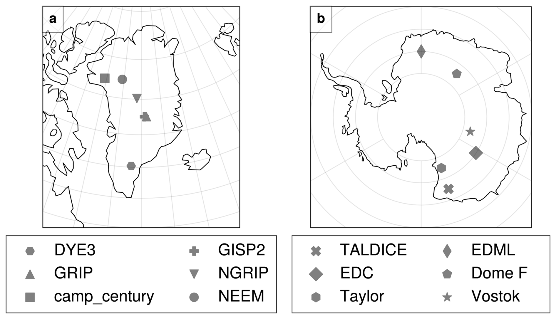
Figure A1 The locations of the Greenland and Antarctic ice core sites.

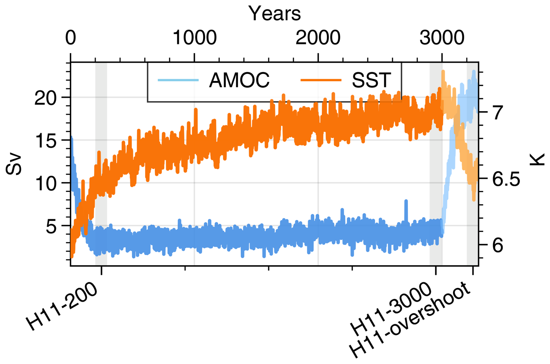
Figure A2 Time series of AMOC (in Sv) and average Southern Hemisphere SST (south of 40° S) time series from HadCM3 H11 simulations. The lighter colours represent the period where the water hosing was stopped. The three grey bands denote the three selected slices from this simulation: H11-200, H11-3000, and H11-overshoot.

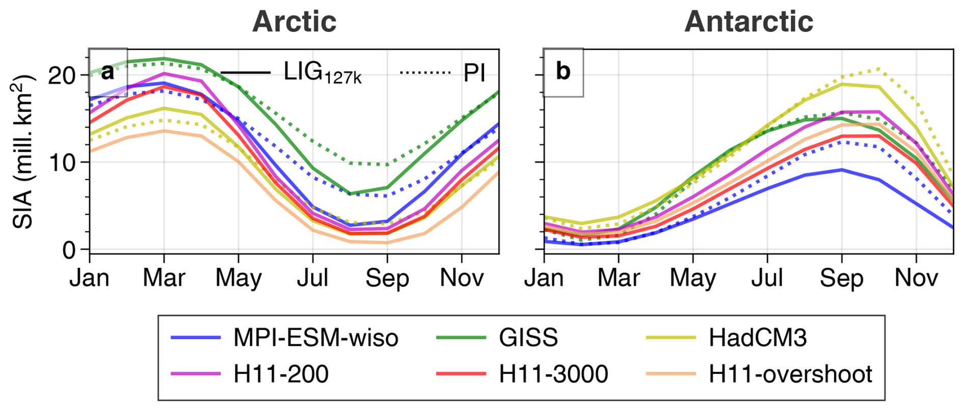
Figure A3 Seasonal cycle of total sea ice area in the Northern and Southern Hemisphere for each simulation. These are absolute values (not Δ values). LIG values are shown using solid lines, and PI values are the dotted lines.

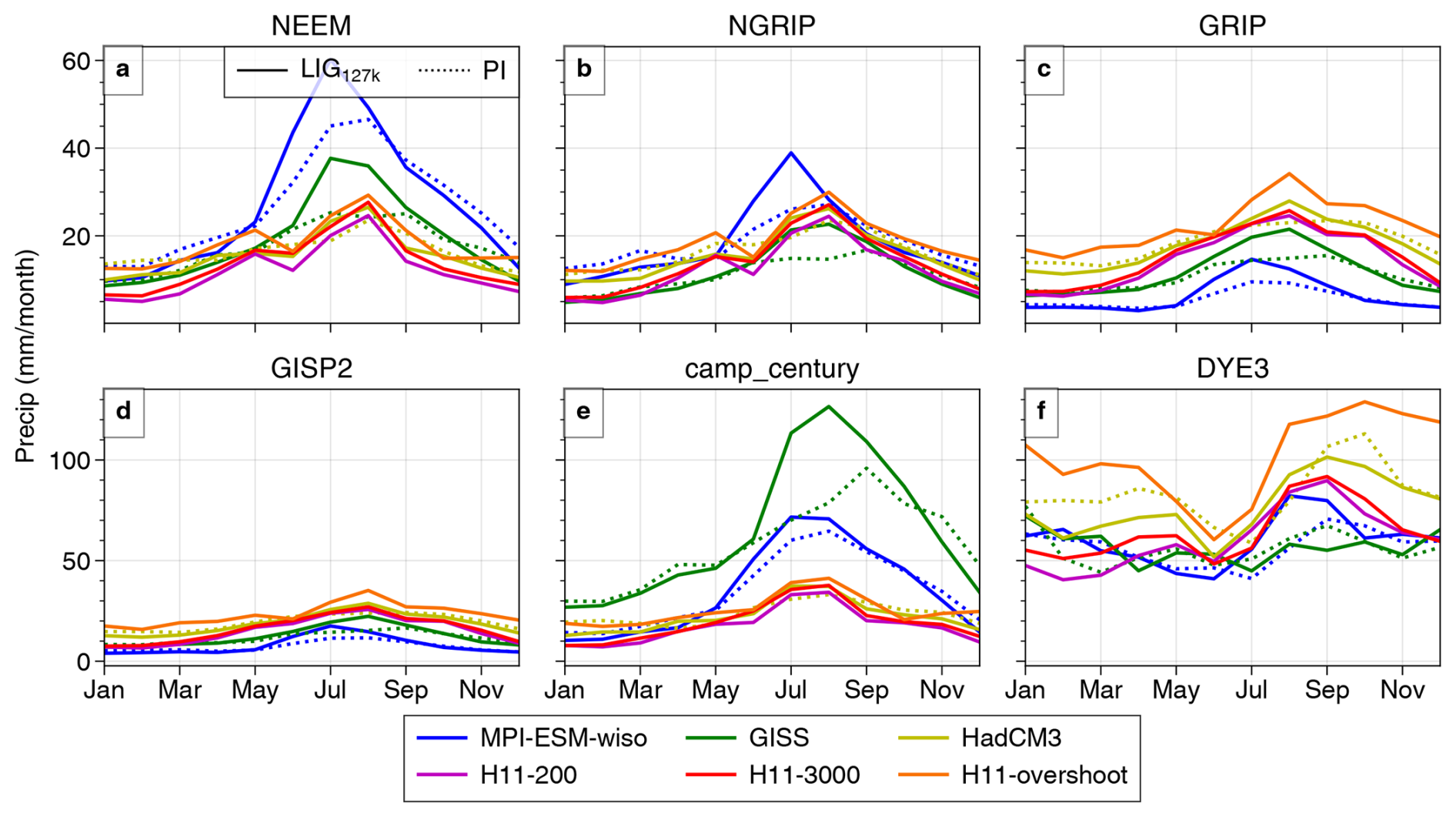
Figure A4 Seasonal cycle of precipitation at each ice core site in Greenland. These are absolute values (not Δ values). LIG values are shown using solid lines, and PI values are the dotted lines.

Figure A5 The seasonal cycle of precipitation, as Fig. A4 but for Antarctica.

Figure A6 The seasonal cycle of δ¹⁸O; otherwise as Fig. A4.

Figure A7 The seasonal cycle of δ¹⁸O for Antarctica; otherwise as Fig. A6.

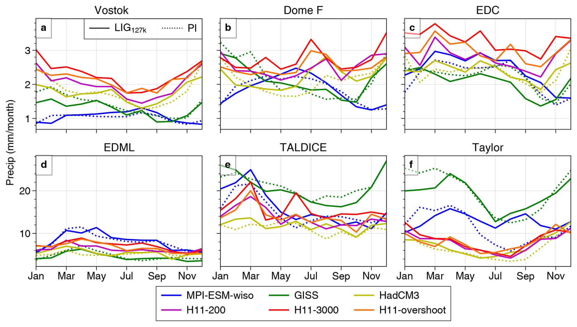
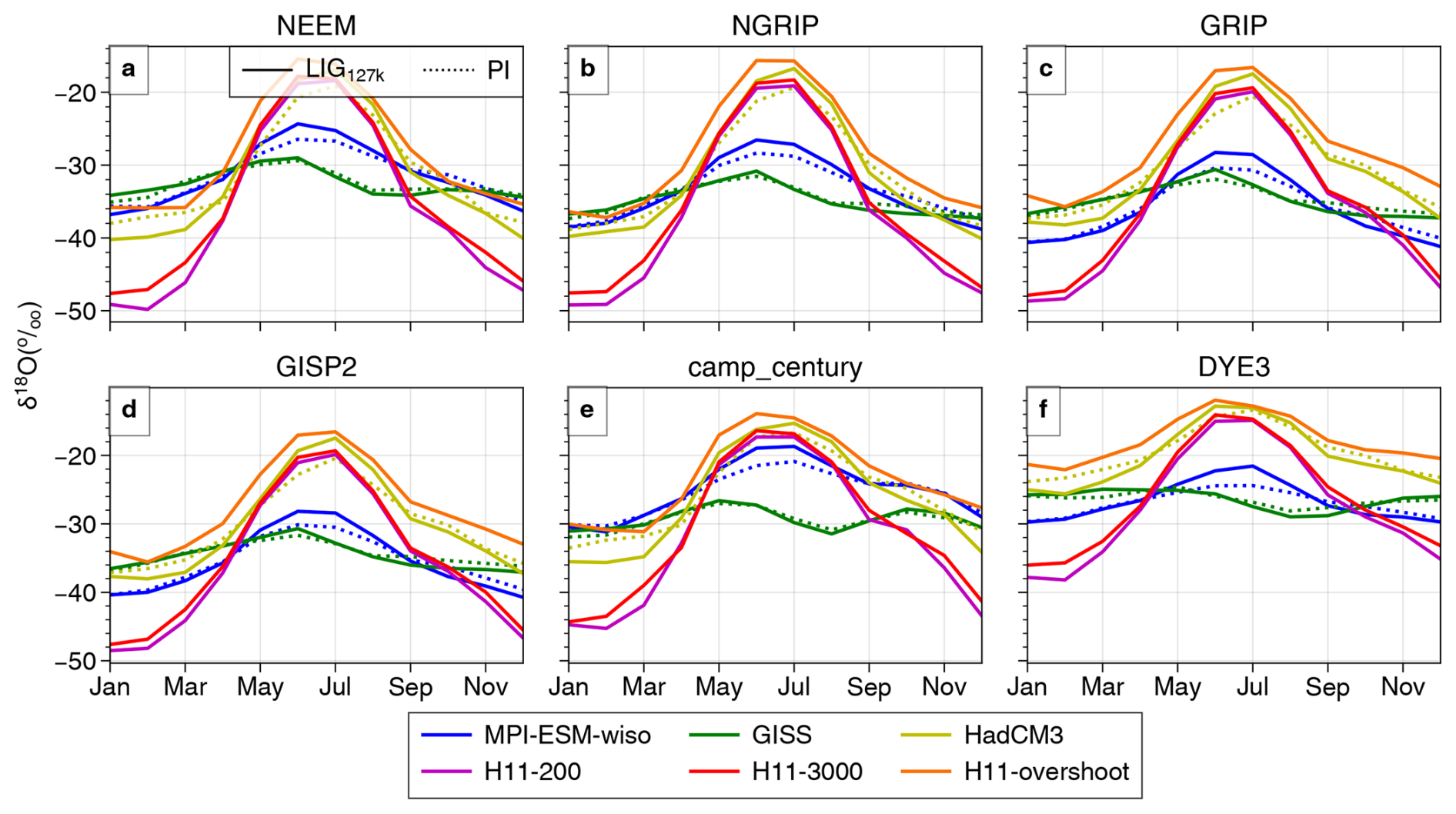
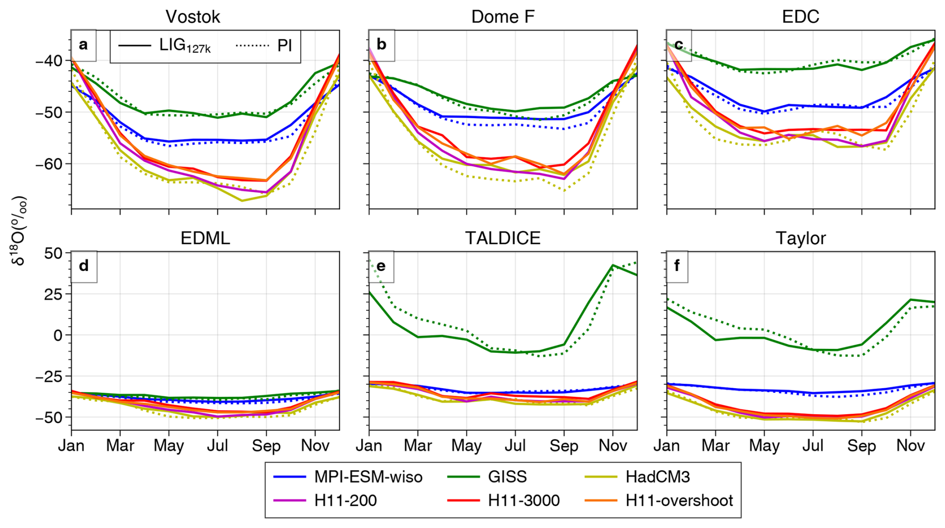
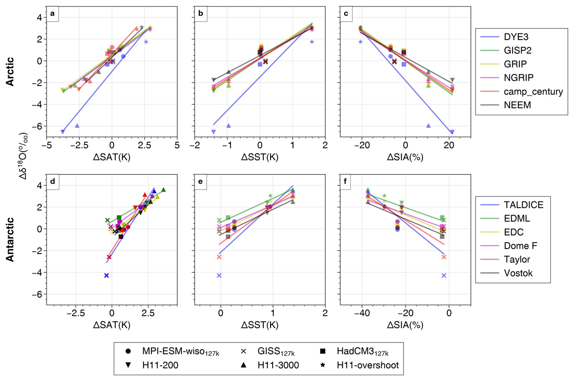
Figure A8 ΔSAT at each ice core location (first column), ΔSST (north/south of 40° latitude for the Arctic and Antarctica), and ΔSIA (annual sea ice area) versus Δδ¹⁸O from each ice core site for all simulations.

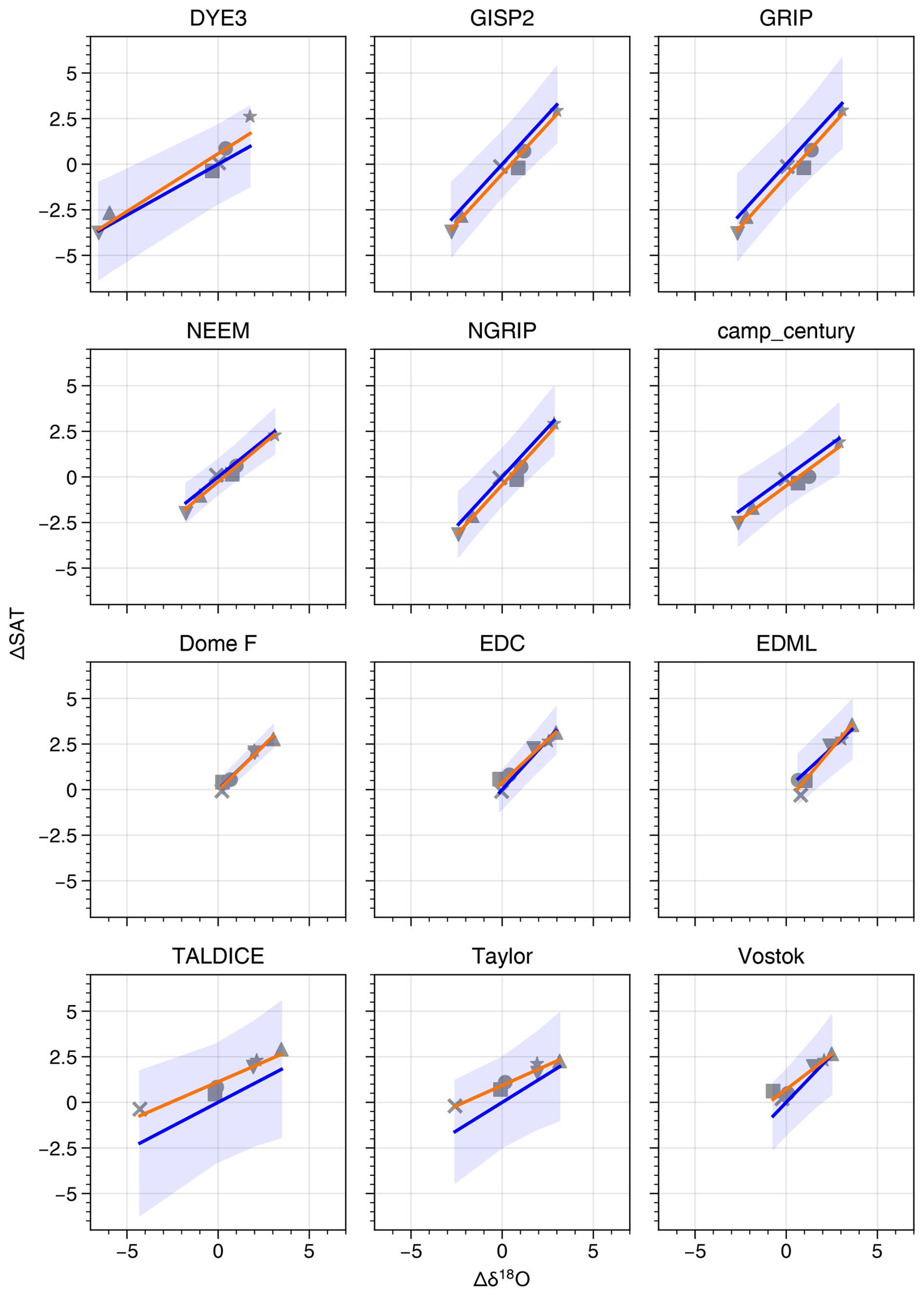
Figure A9 Same as Fig. 11 but using a two-part fit, i.e. a regression line which permits a non-zero intercept (orange lines).

Table A1 Ice core and simulated Δδ¹⁸O values at ice core locations, as well as simulated ΔSAT.

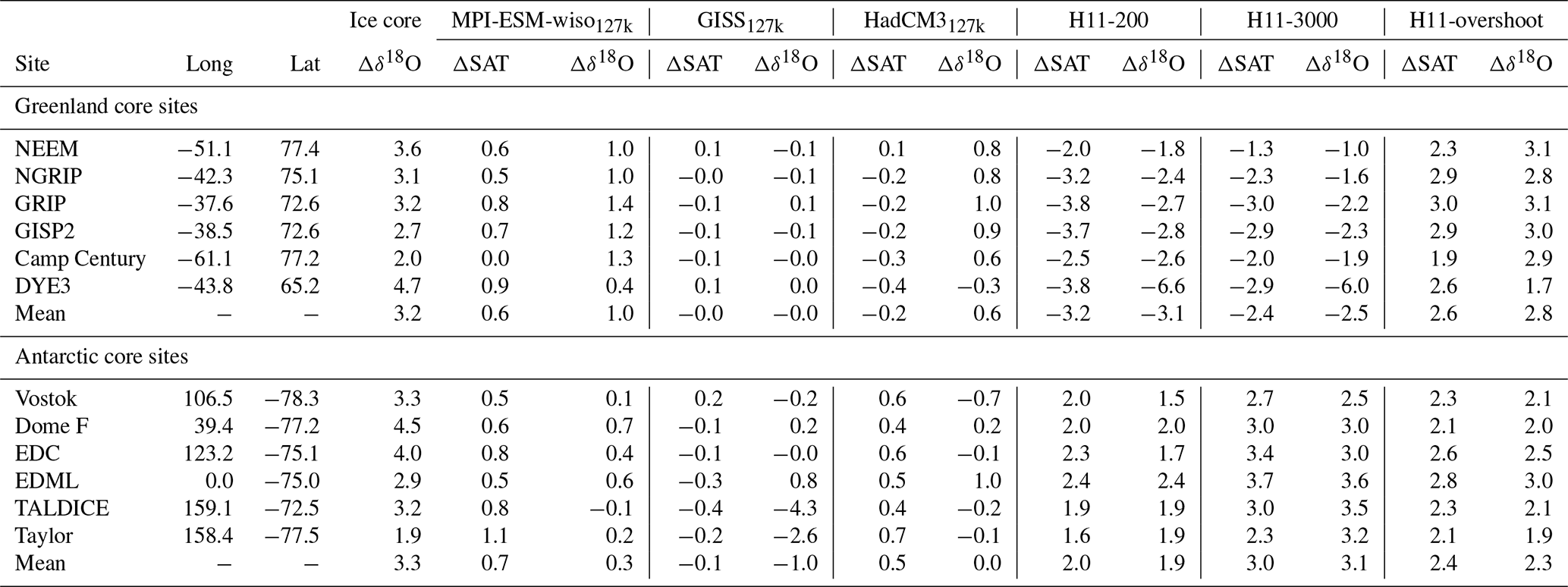
Table A2 Global-mean ΔSAT, ΔSST, and ΔGMOT (global-mean ocean temperature) for each simulation.

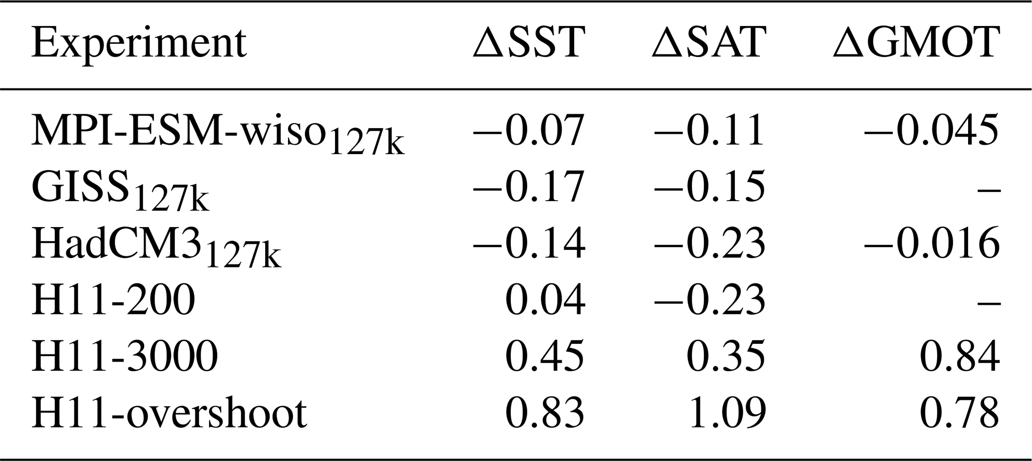
Table A3 Simulated Arctic and Antarctic SAT and SIA values. Column 1: mean ΔSAT (averaged north of 60° N for the Arctic and south of 60° S for Antarctica). Column 2: annual LIG SIA (mill. km²). Column 3: LIG–PI anomaly in SIA (in %). Column 4: summer mean ΔSAT (JJA averaged north of 60° N for the Arctic and DJF south of 60° S for Antarctica). Column 5: seasonal minimum LIG SIA (mill. km²). Column 6: LIG–PI anomaly in seasonal minimum SIA (in %).

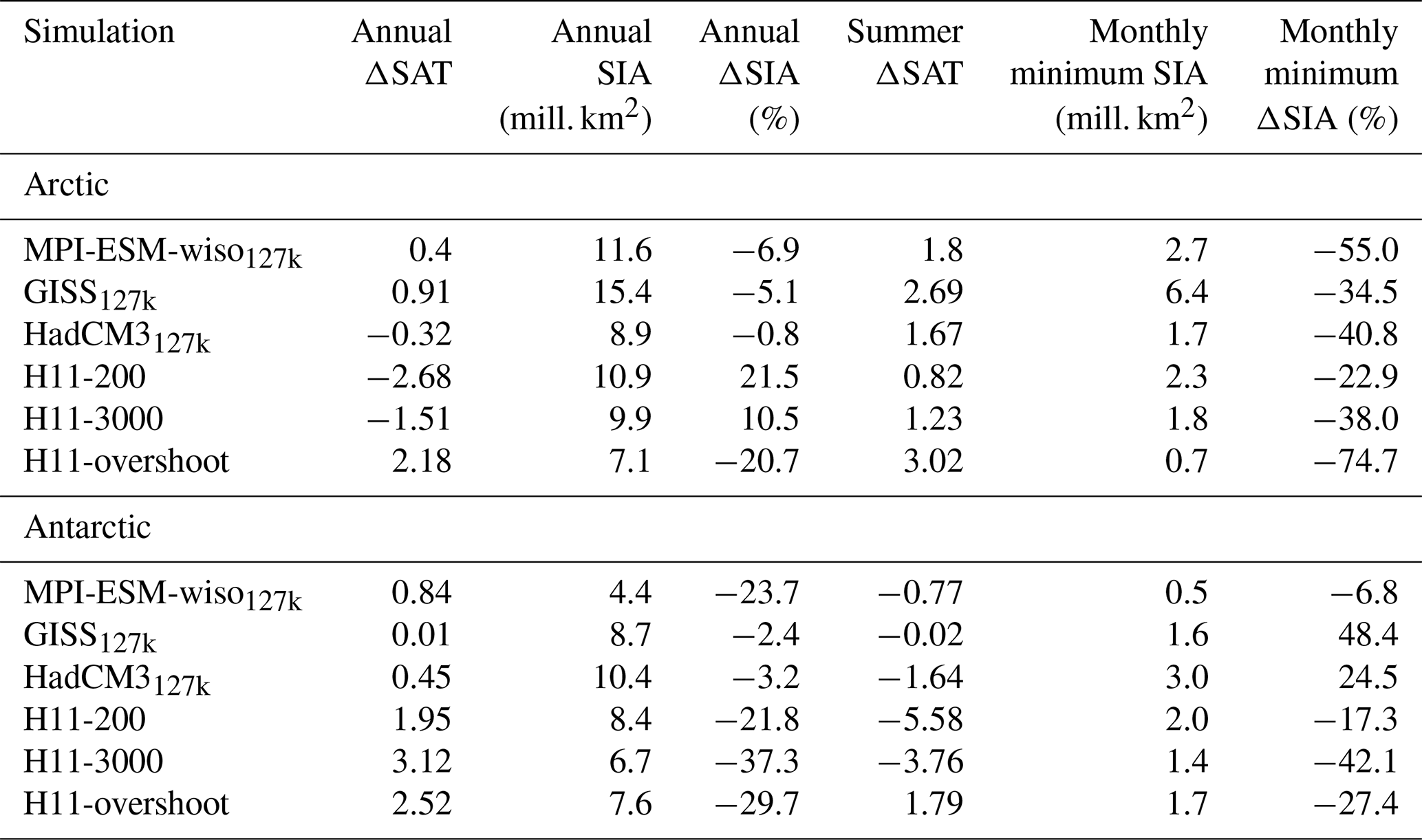
Table A4 Simulated Southern Ocean SST and SIA values, as well as a comparison with equivalent observational syntheses from Gao et al. (2025). Leftmost columns show average annual and summer ΔSST for the Southern Ocean (south of 40° S) for each simulation. Right columns show SST synthesis averages (top row) as compiled by Gao et al. (2025). Lower rows show the percentage of the observed core site ΔSST values achieved by each simulation for each data synthesis. See text and Gao et al. (2025) for details of data synthesis.

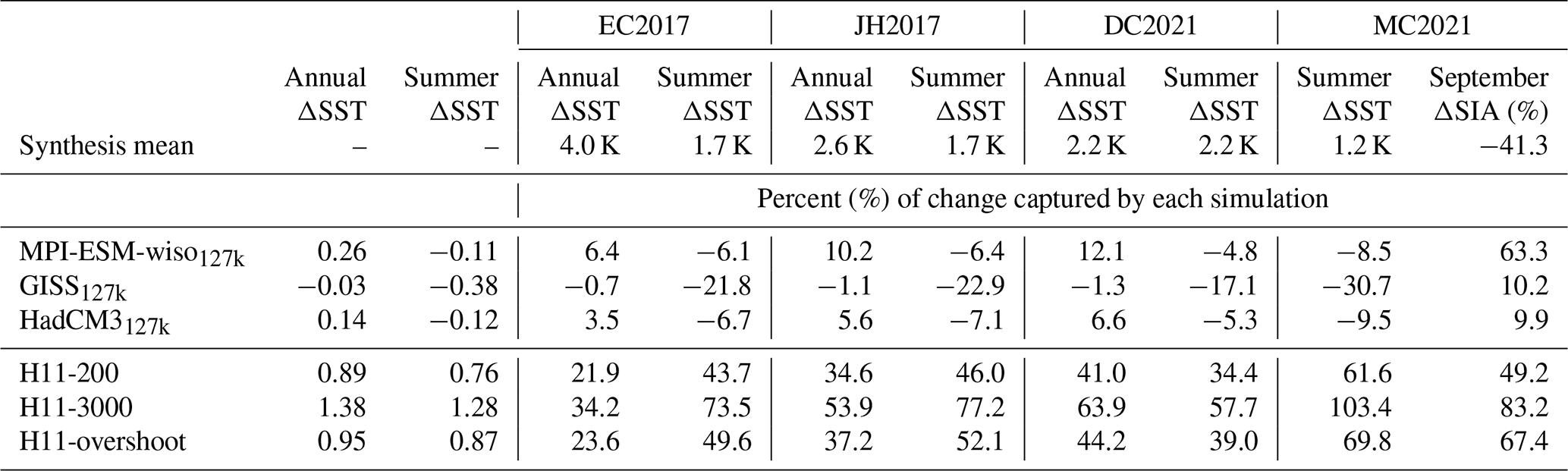
Table A5 Fits and projected ΔSAT values based on ice core Δδ¹⁸O, as Table 2, but based solely on the LIG_127k simulations (H11 results excluded).

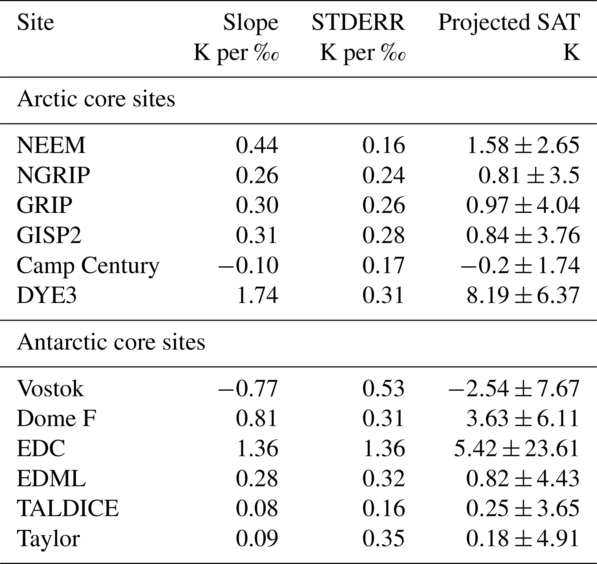
Table A6 Fits and projected ΔSAT values based on ice core Δδ¹⁸O, as Table 2, but based solely on the H11 simulations (LIG_127k results excluded).

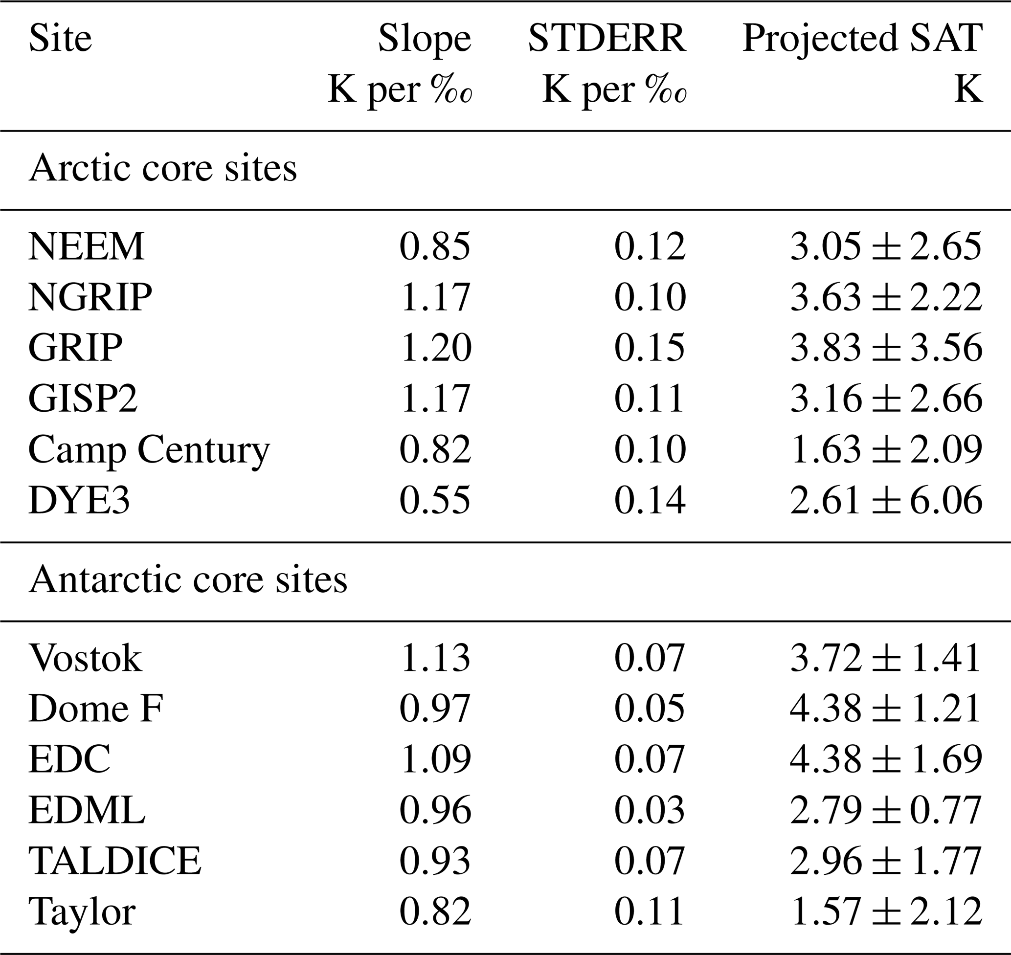
Table A7 This table is as Table 2 but using a two-part regression, i.e. allowing non-zero intercepts. Both the gradient and the intercept are used in the calculation of the projected temperature.