Multi-model assessment of the deglacial climatic evolution at high southern latitudes

The Quaternary climate is characterized by glacial–interglacial cycles, with the most recent transition from the last glacial maximum to the present interglacial (the last deglaciation) occurring between ∼ 21 and 9 ka. While the deglacial warming at high southern latitudes is mostly in phase with atmospheric CO₂ concentrations, some proxy records indicate that the onset of the warming occurred before the CO₂ increase. In addition, high southern latitudes exhibit a cooling event in the middle of the deglaciation (15–13 ka) known as the “Antarctic Cold Reversal”. In this study, we analyse transient simulations of the last deglaciation performed with six different climate models as part of the 4th phase of the Paleoclimate Modelling Intercomparison Project (PMIP4) to understand the processes driving high-southern-latitude surface temperature changes. As the protocol of the last deglaciation sets the choice of freshwater forcing as flexible, the freshwater forcing is different in each model, thus complicating the multi-model comparison. While proxy records from West Antarctica and the Pacific sector of the Southern Ocean suggest the presence of an early warming before 18 ka, only half the models show a significant warming at this time (∼ 1 °C or ∼ 10 % of the total deglacial warming). All models simulate a major warming during Heinrich Stadial 1 (18–15 ka), concurrent with the CO₂ increase and with a weakening of the Atlantic Meridional Overturning Circulation (AMOC) in some models. However, the simulated Heinrich Stadial 1 warming over Antarctica is smaller than the one suggested from ice core data. During the Antarctic Cold Reversal, simulations with an abrupt AMOC strengthening exhibit a high-southern-latitude cooling of 1 to 2 °C, in relative agreement with proxy records, while simulations with rapid North Atlantic meltwater input exhibit a warming. Using simple models to extract the relative AMOC contribution, we find that all climate models simulate a high-southern-latitude cooling in response to an AMOC increase with a response timescale of several hundred years, suggesting the choice of the North Atlantic meltwater forcing substantially affects high-southern-latitude temperature changes. Thus, further work needs to be carried out to reconcile the deglacial AMOC evolution with the Northern Hemisphere ice sheet disintegration and associated meltwater input. Finally, all simulations exhibit only minimal changes in Southern Hemisphere westerlies and Southern Ocean meridional circulation during the last deglaciation. Improved understanding of the processes impacting Southern Hemisphere atmospheric and oceanic circulation changes accounting for deglacial atmospheric CO₂ increase is needed.

1 Introduction

The recent Quaternary climate is characterized by glacial–interglacial cycles with a periodicity of about 100 000 years (Lisiecki and Raymo, 2005; Jouzel et al., 2007). These glacial–interglacial cycles are driven by insolation changes like the external forcing and by internal feedbacks, including changes in atmospheric greenhouse gas concentrations and continental ice sheets (Abe-Ouchi et al., 2013). During the Last Glacial Maximum (LGM, ∼ 21 ka; ka indicates 1000 years before present), the continental ice sheets covered a significant area of the high northern latitudes (Tarasov et al., 2012; Peltier et al., 2015), thus leading to a sea-level fall of ∼ 130 m compared to pre-industrial levels (Lambeck et al., 2014). The atmospheric CO₂ concentration was also ∼ 100 ppm lower than the pre-industrial concentration (Petit et al., 1999; Bereiter et al., 2015). These climatic boundary conditions contributed to a colder climate during the LGM, with global mean surface air temperature anomalies estimated to be 4 to 7 °C lower than the present day (Annan et al., 2022; Liu et al., 2023). As the last deglaciation (transition from the LGM to the early Holocene at ∼ 11 ka) represents one of the largest, most recent and well-documented natural warmings of the last million years, an understanding of the processes and feedbacks during this time period can offer insight into our own modern changing world. Here, we focus on the high southern latitudes, where deglacial warming began before the Northern Hemisphere (NH) counterparts (Shakun et al., 2012); it has been suggested that processes here played a major role in driving the increase in atmospheric CO₂ concentration. Although the timing of the onset of the deglacial warming at high southern latitudes is poorly constrained, a compilation of Antarctic ice core records from East Antarctica suggests that the deglacial Antarctic warming started at ∼ 18 ka, in phase with the rise in atmospheric CO₂ concentration (Parrenin et al., 2013). On the other hand, a record from the West Antarctic Ice Sheet Divide ice core suggests that the warming started at ∼ 20 ka (Shakun et al., 2012; WAIS project members, 2013). Moreover, an early onset of the deglacial warming (∼ 21 ka) at high and mid-southern latitudes has also been inferred from sea surface temperature (SST) and sea ice records from the Pacific sector of the Southern Ocean (Moy et al., 2019; Sikes et al., 2019; Moros et al., 2021; Crosta et al., 2022; Sadatzki et al., 2023).

Millennial-scale climate events are superimposed on the more gradual deglacial warming trend. At the beginning of the deglaciation, during Heinrich Stadial 1 (∼ 18 to 14.7 ka, following Ivanovic et al., 2016), Greenland and the North Atlantic region remained cold (Buizert et al., 2014; Martrat et al., 2007), while significant warming occurred at high southern latitudes (Capron et al., 2010). This period was associated with a weakening of the Atlantic Meridional Ocean Circulation (AMOC), evidenced by Pa $/$ Th in marine sediments (McManus et al., 2004; Ng et al., 2018). During the subsequent Bølling–Allerød period (∼ 14.7 to 12.8 ka), Greenland surface air temperatures rose by more than 10 °C in just a few decades (Steffensen et al., 2008; Buizert et al., 2014), and the AMOC strengthened significantly (Severinghaus and Brook, 1999; McManus et al., 2004; Roberts et al., 2010; Ng et al., 2018). A cooling event at high southern latitudes, known as the Antarctic Cold Reversal, was identified between ∼ 15 and 13 ka (Jouzel et al., 2007; Pedro et al., 2016), concurrent with the Bølling–Allerød. The Younger Dryas (12.8 to 11.7 ka) followed the Bølling–Allerød and was characterized by a drastic cooling in Greenland and the North Atlantic. While the processes leading to the Younger Dryas are still debated (Renssen et al., 2015), it has been suggested that the Younger Dryas could be attributed to a weakening of the AMOC (McManus et al., 2004), caused by a rerouting of freshwater into the Arctic that was then transported toward the deep-water formation sites of the subpolar North Atlantic by coastal boundary currents (Condron and Winsor, 2012; Kapsch et al., 2022). Climate model simulations with marine proxy constraints support the variations in the AMOC during the last deglaciation (Pöppelmeier et al., 2023).

An AMOC weakening causes a warming in the South Atlantic as the meridional oceanic heat transport to the North Atlantic is weakened (Stocker and Johnsen, 2003; Stouffer et al., 2006). This warming can then be propagated to the Southern Ocean and Antarctica (Pedro et al., 2018). The contrasting temperature changes between Greenland and the high southern latitudes can also be found during abrupt events of the last glacial period known as Dansgaard–Oeschger cycles (Dansgaard et al., 1993; North Greenland Ice Core Project Members, 2004; WAIS Divide project members, 2015), leading to the notion of a bipolar seesaw (Stocker and Johnsen, 2003; Capron et al., 2010). Alongside these events, the atmospheric CO₂ increase throughout the deglaciation occurred in steps, suggesting a link with millennial-scale climate events (Marcott et al., 2014) and changes in Southern Ocean circulation contributing to the degassing of oceanic carbon (Anderson et al., 2009; Menviel et al., 2018).

Transient climate simulations provide a suitable framework for assessing the processes leading to deglacial climate changes. Early transient simulations that were conducted with transient orbital forcing, greenhouse gases, and ice sheets suggested that an increase in austral spring insolation at the high southern latitudes was responsible for the onset of warming (Timmermann et al., 2009) and that deglacial warming of the Southern Ocean appeared as early as ∼ 20 to 18 ka in association with sea ice retreat (Roche et al., 2011). Transient simulations that also included freshwater input into the North Atlantic highlighted the AMOC impact on climate change (Liu et al., 2009; He et al., 2013). Menviel et al. (2011) further showed that the Antarctic Cold Reversal could be a response to the strong AMOC increase at the end of Heinrich Stadial 1 but that its length and amplitude could have been enhanced by meltwater input from the Antarctic ice sheet. These simulations were designed to simulate AMOC changes in agreement with estimates from proxy records, and therefore the magnitude, location, and timing of the implemented meltwater fluxes were idealized. In contrast, experiments forced with meltwater fluxes consistent with ice sheet reconstructions based on sea-level constraints often simulate millennial-scale AMOC changes in disagreement with accepted interpretations of climate and ocean records (Snoll et al., 2024). Some experiments simulate an AMOC weakening at the time of the Bølling–Allerød because of significant mass loss of Northern Hemisphere ice sheets (Bethke et al., 2012; Ivanovic et al., 2018; Kapsch et al., 2022; Bouttes et al., 2023) or do not simulate any abrupt climate events (Gregoire et al., 2012). With an idealized scenario that follows the evolution of Northern Hemisphere ice sheets more closely (except for the 14 ka meltwater pulse), the MIROC climate model shows that it is possible to simulate an abrupt AMOC strengthening with the presence of continuous freshwater in the North Atlantic because of gradual warming (Obase and Abe-Ouchi, 2019). These studies indicate that different models have different sensitivities in terms of the AMOC response to forcing, and, therefore, it is useful to analyse multi-model results for a robust understanding of the climatic processes.

To facilitate further examination of the mechanisms driving deglacial climate change, a protocol for carrying out transient simulations of the last deglaciation was proposed as part of the 4th phase of the Paleoclimate Modeling Intercomparison Project (PMIP4) (Ivanovic et al., 2016). The PMIP4 last deglaciation model protocol summarized the climate forcings needed (ice-core-based atmospheric greenhouse gases and reconstructed ice sheets) for climate model experiments. The protocol is designed to be flexible in that the use of some boundary conditions is determined by each modelling group, which allows an exploration of different climate scenarios. The first PMIP multi-model study of the last deglaciation, focusing on the northern hemispheric climate during Heinrich Stadial 1, found that different freshwater approaches (melt-uniform, melt-routed, TraCE-like, bespoke; Snoll et al., 2024) have a dominant impact on North Atlantic climate variability. The multi-model assessment of the last deglaciation performed here provides an opportunity to investigate the processes impacting high-southern-latitude climate and to evaluate model sensitivity to the forcings.

Some boundary conditions for climate models, including greenhouse gases and Antarctic ice sheet (prescribed in the PMIP4 protocol), result from climate change at high southern latitudes. Proxy records (Sigman et al., 2010; Skinner et al., 2010; Martínez-Garcia et al., 2011) and modelling studies (Bouttes et al., 2012; Menviel et al., 2017, 2018; Gottschalk et al., 2019) indicate that physical and biogeochemical changes in the Southern Ocean may have significantly contributed to ocean carbon uptake during the last glacial period and to the atmospheric CO₂ increase during Heinrich Stadial 1. Subsurface warming on the Antarctic shelf contributes to the mass loss of Antarctic ice sheets through enhanced melting of ice shelves and retreat of grounding lines (Golledge et al., 2014; Lowry et al., 2019). In addition, climate conditions at high southern latitudes can impact the formation of Antarctic Bottom Water and the shoaling of AMOC (Sherriff-Tadano et al., 2023). Hence investigating the deglacial climate evolution at high southern latitudes may provide insight into critical climate system feedbacks.

Here, we analyse the deglacial climatic evolution (21–11 ka) at high southern latitudes as simulated in six PMIP4 transient experiments and compare the results with paleo-proxy records. We focus on the magnitude and rate of changes in Antarctic surface air temperature (SAT) and Southern Ocean SST. As there is a substantial difference between the temporal evolution of AMOC strength in the simulations, we utilize statistical or simple models to separate the impact of changes in atmospheric CO₂ and AMOC on Southern Ocean SST. Finally, we analyse the evolution of Antarctic Bottom Water, Southern Ocean westerlies, and subsurface ocean temperature to discuss critical climate system feedbacks occurring at high southern latitudes.

2 Methods

2.1 Climate models and experiments used in this study

We use the PMIP4 transient simulations of the last deglaciation performed with six atmosphere–ocean coupled climate models (Table 1) and analyse the time period from the LGM to the Early Holocene, 21–11 ka. Table 2 summarizes the experimental design of each model and describes the simulation (including LGM and pre-industrial climates). The LGM climate fields (initial condition of these experiments) have been evaluated by previous studies, particularly for global temperature changes (Kageyama et al., 2021), sea ice and SST changes in the Southern Ocean (Lhardy et al., 2021; Green et al., 2022), and SAT changes over the Antarctic ice sheet (Buizert et al., 2021). A part of the transient simulations utilized in this study have also been compared to proxy reconstructions (Weitzel et al., 2024). Figure S1 in the Supplement compares simulated sea ice edges for the pre-industrial simulations from six models used in this study, showing that some models underestimate pre-industrial summer sea ice extent but mostly to an acceptable level. The equilibrium climate sensitivity (ECS, defined by global mean SAT changes in response to doubling CO₂ from the pre-industrial level) of each model ranges from 2.0 to 3.9 °C, and the global mean surface air temperature (SAT) anomaly for the LGM is 3.5 to 7.3 °C (Table 1).

Table 1 Summary of climate models analysed in this study. Note that the ECS for MPI-ESM (model version MPI-ESM-CR P2) has not been calculated.

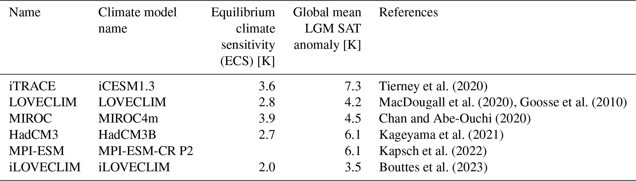
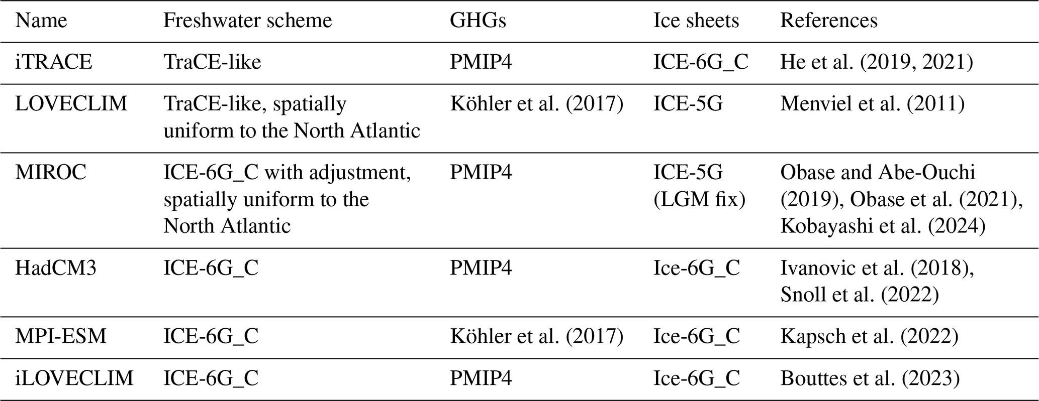
Table 2 Summary of the experimental design used in the transient deglacial simulations. PMIP4 in the column GHGs indicates they use three greenhouse gases reconstructions (CO₂, CH₄, N₂O) in the PMIP4 protocol paper (Ivanovic et al., 2016).

While some of the modelling groups performed two or more sensitivity experiments with different model parameters or boundary conditions (e.g. different freshwater forcing scenarios or ice sheets), for this study we have selected one representative simulation from each climate model. Figure 1 summarizes the time evolution of the climate forcings, i.e. insolation, atmospheric greenhouse gases, and continental ice sheets, used in the simulations. Both the PMIP4-recommended reconstructions (ICE-6G_C VM5a, henceforth “ICE-6G_C”, and “GLAC-1D”) have larger Antarctic ice sheet volume at the LGM, with a ∼ 10 m sea-level-equivalent volume change at the LGM relative to the present day. Both suggest ∼ 100 m of elevation reduction since the LGM at EPICA Dome C (EDC; 123° E, 75° S), while estimates of the elevation change at the West Antarctic Ice Sheet Divide (WDC; 112° W, 79.5° S) differ by 300 m between the two datasets (Fig. 1d).

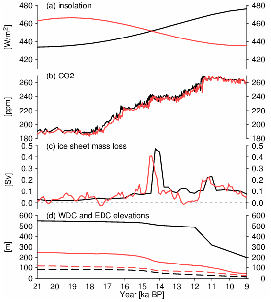
Figure 1 Forcing of the last deglaciation. (a) Insolation based on Berger (1978). Black: 65° N July; red: 65° S January. (b) CO₂. Black: Bereiter et al. (2015); red: Köhler et al. (2017). (c) Freshwater forcing in the NH from ICE-6G_C (black lines) and GLAC-1D (red lines). (d) Elevation change at WDC (bold lines) and EDC (dashed lines) from ICE-6G_C (black lines) and GLAC-1D (red lines).

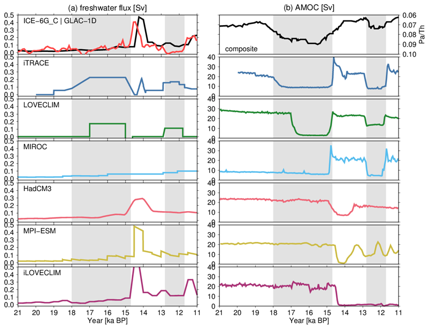
Figure 2 (a) Freshwater forcing (total value in the NH) and (b) simulated AMOC time series. The top panels indicate the freshwater flux from ice sheet reconstructions (black indicates ICE-6G_C and red indicates GLAC-1D) and composite ²³¹Pa $/$ ²³⁰Th in the North Atlantic, retrieved from Ng et al. (2018). The top three model panels correspond to the first group with freshwater forcing adjusted to reproduce large-scale AMOC variability, and the bottom three model panels correspond to the second group with freshwater forcing consistent with the reconstructed ice volume changes. The grey shading from left to right indicates Heinrich Stadial 1 (18–14.7 ka) and the Younger Dryas (12.8–11.7 ka), and the period in between corresponds to the Bølling–Allerød (14.7–12.8 ka).

Figure 2a summarizes the total amount of freshwater forcing in the Northern Hemisphere in six simulations. The freshwater forcing schemes can be classified into two groups: the first group characterizes freshwater forcing that has been adjusted to reproduce large-scale AMOC variability (utilized in iTRACE, LOVECLIM, and MIROC simulations), and the second group includes freshwater forcing consistent with the reconstructed ice volume changes (implemented in HadCM3, MPI-ESM, iLOVECLIM simulations) based on ICE-6G_C or GLAC-1D (Fig. 2a, upper panel, red and black lines). Notably, during Heinrich Stadial 1, iTRACE and LOVECLIM have significant freshwater forcing (∼ 0.2 Sv), while other simulations (including MIROC) apply freshwater forcing of less than 0.1 Sv. In LOVECLIM and MIROC, the meltwater flux was uniformly applied to the North Atlantic, while other models use the location of ice sheet melting and associated runoff distribution to apply a spatially varying freshwater forcing (Table 2). ICE-6G_C (HadCM3, MPI-ESM, iLOVECLIM) leads to a meltwater input of about 0.1 Sv to the Southern Ocean at 11.5–11 ka. iTRACE and LOVECLIM also applied a freshwater flux to the Southern Ocean to simulate the Antarctic Cold Reversal (iTRACE: up to 0.2 Sv during 14.4–13.9 ka; LOVECLIM: fixed at 0.09 Sv during 14.67–14.1 ka).

Furthermore​​​​​​​, we conduct further analysis to examine the processes driving Southern Ocean SST change using a multilinear regression (MLR) model and a thermal bipolar seesaw model adapted from Stocker and Johnsen (2003).

2.2 Simple models for disentangling CO₂ and AMOC

2.2.1 Multilinear regression model

We use a MLR model to regress changes in SST onto CO₂ and AMOC variations:

$$\begin{array}{}\text{(1)}& \mathrm{SST}={\mathit{\alpha }}_{\mathrm{1}}\times {\mathrm{CO}}_{\mathrm{2}}+{\mathit{\beta }}_{\mathrm{1}}\times \mathrm{AMOC}+\mathit{\gamma },\end{array}$$

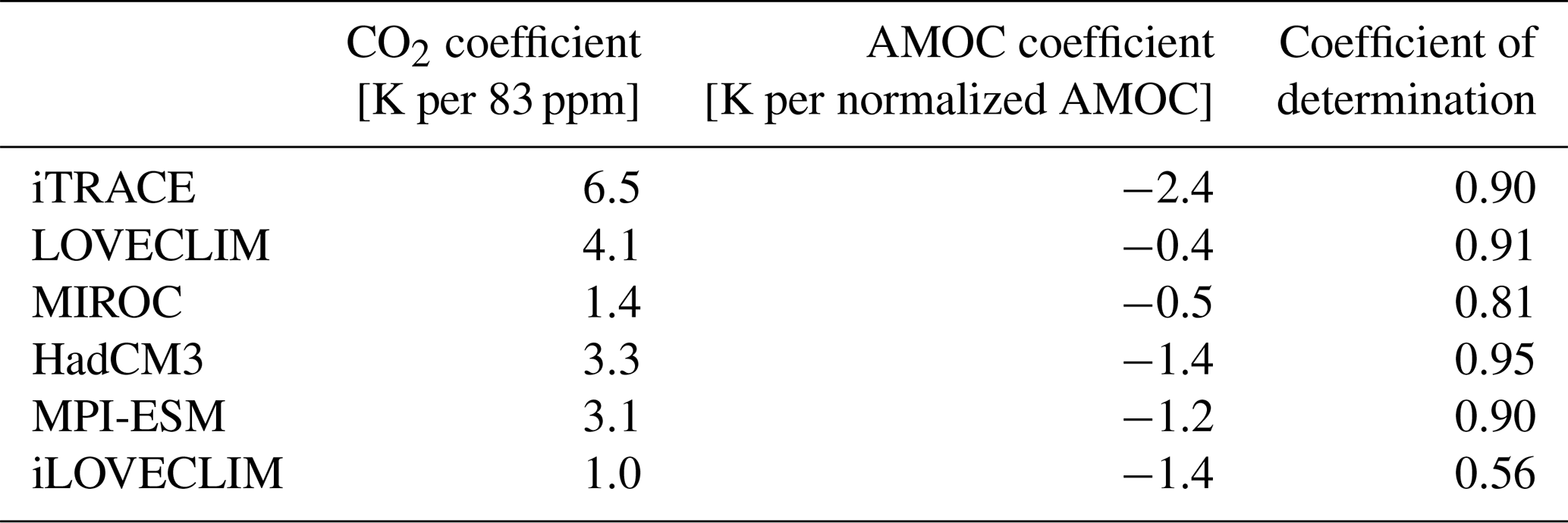
where SST and AMOC (defined as the maximum meridional overturning streamfunction in the North Atlantic, at depths below 500 m and 20–60° N) are output from the climate models, CO₂ is the forcing used in each simulation, and γ is the intercept. The AMOC in the analysis is normalized with respect to the temporal maximum and minimum values in each model. The CO₂ is also normalized with respect to the total change between 21 and 11 ka (∼ 83 ppm). The MLR analysis is applied to the 2-D fields of the Southern Ocean SST. The same analysis is applied to the Southern Ocean SST averaged over 55–40° S. To focus on long-term climate change and reduce interannual variability, every 100 years, mean SST, AMOC, and CO₂ from 20 to 11 ka are used as the input for this analysis, so each dataset has 90 time slices. While we use CO₂ as a representation of a gradual forcing as the input of the MLR model, we note that other forcings, such as from ice sheets and orbital changes, can contribute to the warming. On the other hand, sensitivity experiments evaluating the contribution of each forcing show that they have a minor impact on Southern Ocean SST and Antarctic SAT changes between 19 and 15 ka (He et al., 2013). The results with coefficients of determination are displayed in Table 3.

Table 3 Results of the MLR model for Southern Ocean SST.

2.2.2 Thermal bipolar seesaw model

As the MLR model does not consider the transient climate response, we construct a thermal bipolar seesaw model following Stocker and Johnsen (2003). The original thermal bipolar seesaw model is based on the energy balance between the North and South Atlantic oceans. We add the effect of CO₂ on temperature, which was not considered in the original model. Thus, the thermal bipolar seesaw model in this study solves the temporal evolution of Southern Ocean SST using the following equations:

$$\begin{array}{}\text{(2)}& {\displaystyle \frac{\mathrm{d}\mathrm{\Delta }\mathrm{SST}}{\mathrm{d}t}}={\displaystyle \frac{\mathrm{\Delta }\mathrm{SSTeq}-\mathrm{\Delta }\mathrm{SST}\left(t\right)}{\mathit{\tau }}},\text{(3)}& {\displaystyle }\mathrm{\Delta }\mathrm{SSTeq}={\mathit{\alpha }}_{\mathrm{2}}\times {\mathrm{CO}}_{\mathrm{2}}\left(t\right)+{\mathit{\beta }}_{\mathrm{2}}\times \mathrm{AMOCm}\left(t\right),\end{array}$$

where ΔSSTeq is an equilibrium Southern Ocean SST (change since the LGM) expected from the CO₂ and state of the AMOC at time t. ΔSST(t) is the SST change since the LGM at time t, and τ is the characteristic timescale of the bipolar seesaw. CO₂(t) is the CO₂ concentration at time t and is normalized with maximum and minimum values as in the MLR model. The term AMOCm(t) represents the modes of the AMOC from the climate model outputs. When using the simulated AMOC within the bipolar seesaw model, it is assumed that the AMOC modes are binary, unlike the continuous values in the model. Based on Fig. 2, we assume that the AMOC is in a strong mode (AMOCm(t)=0) if the AMOC is greater than 14 Sv.

At first, we conduct systematic sensitivity experiments to calculate the minimum root mean square error between the actual ΔSST and the bipolar seesaw model. We conduct 9610 sensitivity experiments for each model within the parameter ranges shown in Table 4. The combination of parameters that gives the minimum root mean square error, along with the coefficient of determination between the climate models' SST changes and bipolar seesaw models, is displayed in Table 5.

Table 4 Parameter ranges in the thermal bipolar seesaw model.

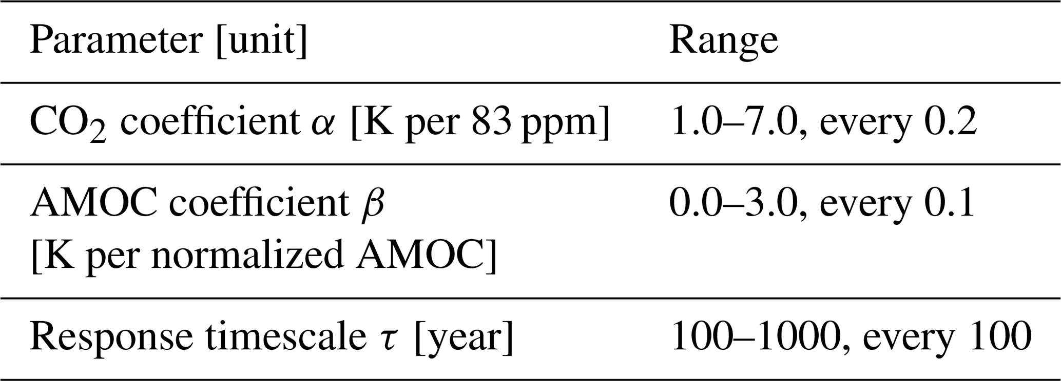
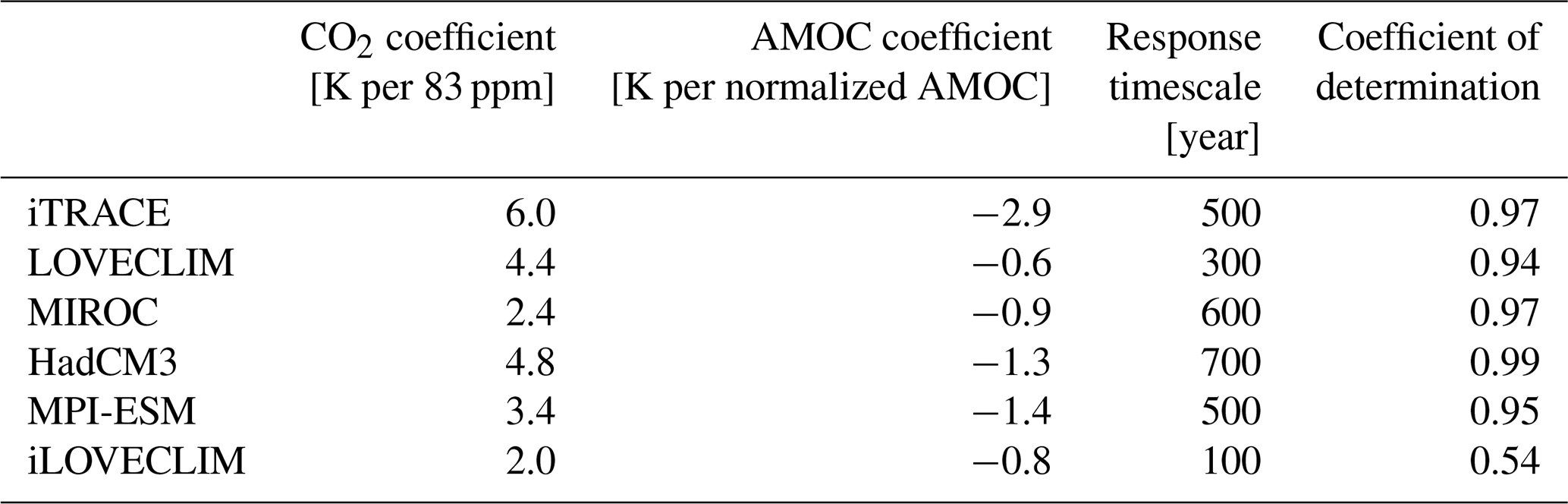
Table 5 Results of the bipolar seesaw model for Southern Ocean SST.

3 Results

3.1 AMOC

As AMOC variations can impact high-southern-latitude climate, we summarize here the transient evolution of the AMOC in the different simulations. As detailed below, the AMOC evolution is substantially affected by the freshwater forcing schemes. All simulations except for MIROC display a strong (∼ 20 Sv) AMOC at the LGM (Fig. 2b), although we note that MPI-ESM and iLOVECLIM simulate a slightly weaker LGM AMOC in their sensitivity tests using the GLAC-1D ice sheet instead of ICE-6G_C (Kapsch et al., 2022; Bouttes et al., 2023). The more vigorous LGM AMOC compared to the pre-industrial period is in line with the majority of the PMIP4 simulations (Kageyama et al., 2021), although it is not consistent with LGM reconstructions from multiple marine tracers (Lynch-Stieglitz et al., 2007; Böhm et al., 2015; Menviel et al., 2017).

During the period corresponding to Heinrich Stadial 1, the AMOC stays weak in MIROC and substantially declines in the iTRACE and LOVECLIM simulations as meltwater is added into the North Atlantic. On the other hand, in the other simulations, there is only a slight reduction in AMOC (∼ 1 Sv) as the meltwater input into the North Atlantic stays below 0.05 Sv. At the transition to the Bølling–Allerød (∼ 14.7 ka), three models exhibit an abrupt change from weak to strong AMOC, triggered by a rapid reduction in freshwater forcing (iTRACE and LOVECLIM) or as a response to the gradual background warming (MIROC). These simulations, featuring an AMOC strengthening, broadly agree with marine proxy records (Fig. 2b black line). On the other hand, the other three simulations (HadCM3, MPI-ESM, iLOVECLIM) display an AMOC weakening due to a substantial increase in Northern Hemisphere freshwater forcing originating from the ice sheet collapse associated with Meltwater Pulse 1a (Deschamps et al., 2012). During the Younger Dryas (12.8–11.7 ka), iTRACE, LOVECLIM, and MIROC simulate a weakened AMOC state compared to the Bølling–Allerød, corresponding to an increase in freshwater forcing (iTRACE, LOVECLIM) or, in the case of MIROC, due to being in an oscillatory regime (Kuniyoshi et al., 2022). HadCM3 simulates a small but gradual AMOC reduction throughout the Younger Dryas, while MPI-ESM exhibits multi-centennial AMOC variability. At 11 ka, the AMOC returns to a strong mode except for iLOVECLIM, which stays weak after the Bølling–Allerød.

3.1.1 21–18 ka (onset of warming) and 18–14.7 ka (Heinrich Stadial 1)

​​​​​​​Figure 3 summarizes the changes in Antarctic SAT (Fig. 3c–d) and Southern Ocean SST (Fig. 3e) since the LGM in all the simulations (LGM is defined as 21 ka in most models, with some exceptions because of different initialization: 20.0 ka for iTRACE, 20.6 ka for LOVECLIM). The SAT at WDC and EDC are compared with the ice-core-based reconstructions from Parrenin et al. (2013) and Buizert et al. (2021). Three models (MIROC, HadCM3, MPI-ESM) exhibit a gradual ∼ 1 °C warming between 21 and 18 ka at both WDC and EDC (Fig. 3c). The simulated EDC warming is comparable to ice core estimates, with MPI-ESM overestimating the warming at the EDC site (Fig. 4a). However, the magnitude of warming suggested by WDC ice core data (∼ 2 °C warming between 19.5–19 ka; Shakun et al., 2012) is not fully simulated by any of the models, with iTRACE even exhibiting slight cooling (Fig. 4a). MIROC, HadCM3, and MPI-ESM simulate a SAT increase over Antarctica and a 0.5–1.0 °C SST increase in the Southern Ocean north of the sea ice edge, with a gradual reduction in Southern Ocean sea ice area (Figs. 3f and 4b).

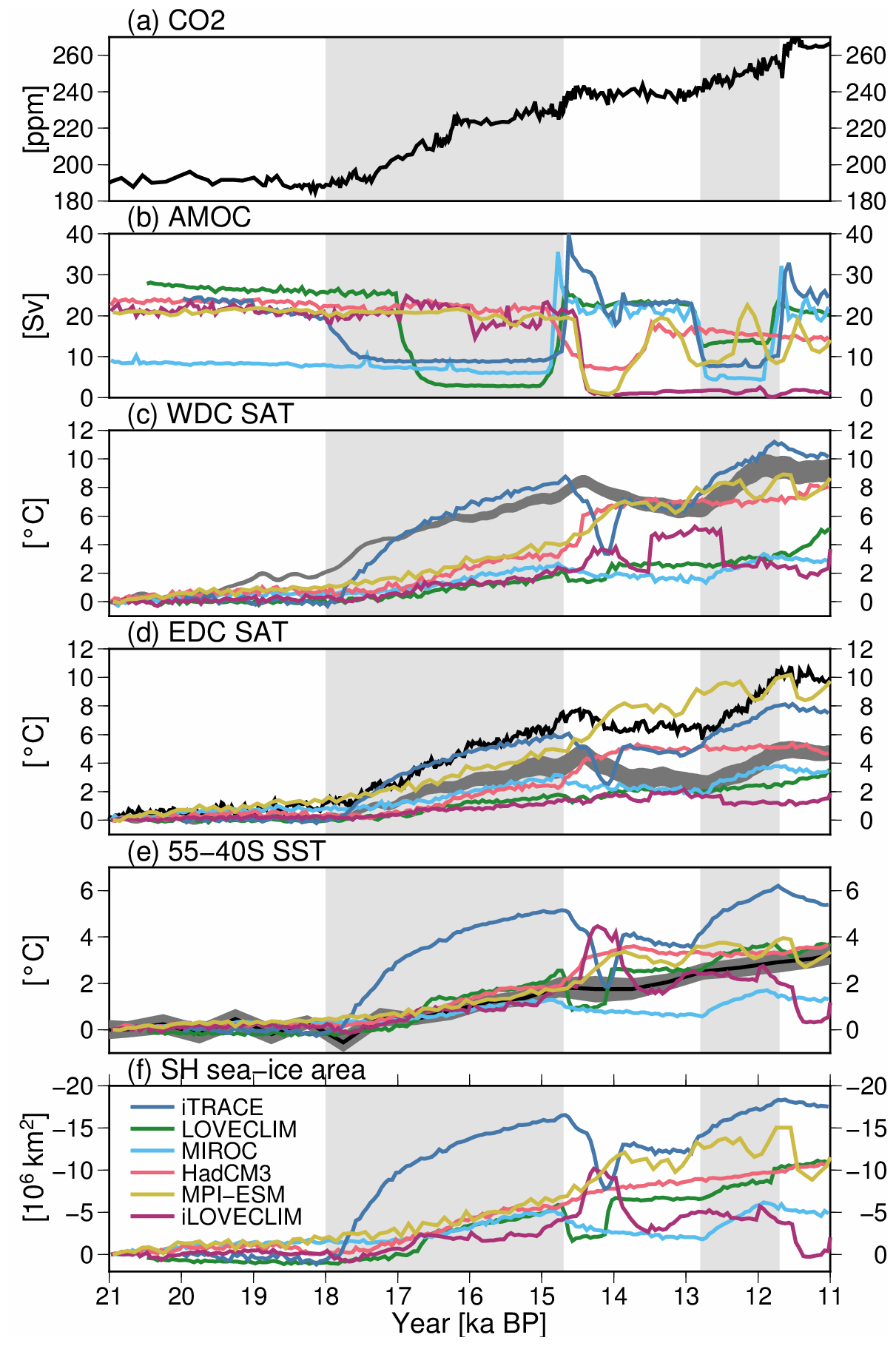
Figure 3 Time series of (a) atmospheric CO₂ (Bereiter et al., 2015), (b) simulated AMOC, (c–d) SAT at WDC and EDC, (e) Southern Ocean SST (zonal mean SST in the latitude band 55–40° S), and (f) Southern Ocean sea ice area in the transient simulations. The SAT, SST, and sea ice area indicate changes since the LGM. The grey lines in panels (c)–(d) represent reconstructions from Buizert et al. (2021), and the black line in panel (d) represents reconstructions from Parrenin et al. (2013). The black lines and grey shades in panel (e) indicate the Southern Ocean SST stack and its standard error, respectively, as derived by Anderson et al. (2020). The vertical grey shading from left to right indicates Heinrich Stadial 1 (18–14.7 ka) and the Younger Dryas (12.8–11.7 ka), and the period in between corresponds to the Bølling–Allerød (14.7–12.8 ka).

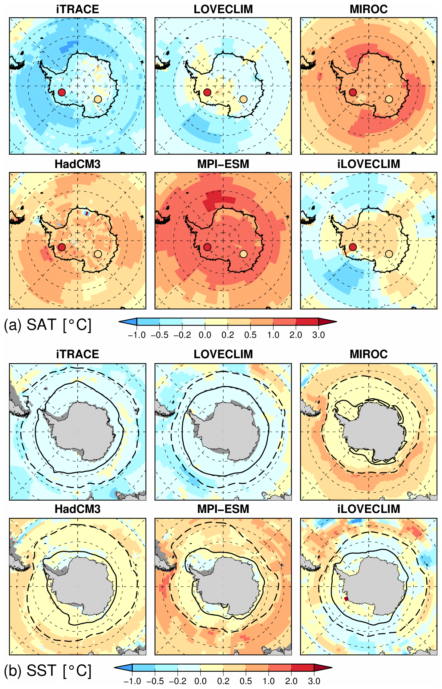
Figure 4 (a) SAT and (b) SST anomalies at 18 ka compared to the LGM. The coloured circles in panel (a) represent 18 ka LGM SAT change based on ice core data (Parrenin et al., 2013), and the bold and dashed lines in panel (b) represent LGM austral summer and winter sea ice extent (85 % and 15 % annual-mean sea ice concentration), respectively.

All models exhibit a larger warming between 18 and 14.7 ka (i.e. Heinrich Stadial 1) than between 21 and 18 ka. iTRACE simulates the largest warming in SAT at WDC and EDC (+6–8 °C, Fig. 3c–d), closely following the estimates from ice core data. The sharp increase in temperature in iTRACE starts at ∼ 18 ka, corresponding to a period of major reduction in AMOC strength (Fig. 3b). The warming in MPI-ESM follows iTRACE with a 5 °C warming despite a minor reduction in AMOC strength. HadCM3 exhibits a ∼ 4 °C warming at WDC and a ∼ 2 °C warming at EDC, while the other models simulate a 2–4 °C warming at EDC and WDC (Fig. 3c–d). iTRACE exhibits a Southern Ocean SST increase of 5 °C, and LOVECLIM exhibits a sharp Southern Ocean SST increase of ∼ 3 °C, in response to an AMOC reduction at ∼ 17 ka. The other models' Southern Ocean SSTs increase by 1–2 °C (Fig. 3e). Southern Ocean sea ice area exhibits the same trends as the Southern Ocean SST, with iTRACE simulating the largest sea ice area reduction of up to 40 % compared to the LGM (Fig. 3f), noting that iTRACE has the largest LGM sea ice extent (Fig. 4b).

3.1.2 14.7–13 ka (Bølling–Allerød) and 13–11 ka (Younger Dryas and Holocene onset)

Three models (iTRACE, LOVECLIM, MIROC) simulate an abrupt AMOC increase at the onset of the Bølling–Allerød (Fig. 3b) and a concomitant cooling at high southern latitudes: a decrease of ∼ 1–2 °C in Antarctic SAT and Southern Ocean SST (Fig. 3c–e). iTRACE and LOVECLIM exhibit a sharp cooling in Southern Ocean SST and SAT in the early phase of the Bølling–Allerød (Fig. 3e), probably enhanced by the meltwater flux into the Southern Ocean (Menviel et al., 2011). In contrast, the three other models (HadCM3, MPI-ESM, iLOVECLIM) exhibit a warming in the early phase of the Bølling–Allerød, corresponding to their AMOC weakening. Subsequently, HadCM3 and MPI-ESM exhibit a gradual cooling over the Antarctic and Southern Ocean as the AMOC strengthens in the later part of the Bølling–Allerød (∼ 13.5 ka). iLOVECLIM displays a rapid warming at 13.5 ka, followed by a cooling, which is explained by abrupt surface albedo changes caused by the evolving land–sea mask in the Antarctic region (Bouttes et al., 2023).

During the Younger Dryas (13–11 ka), iTRACE, LOVECLIM, and MIROC simulate an AMOC weakening as well as a high-southern-latitude warming. iTRACE simulates a ∼ 3–4 °C increase in Southern Ocean SST, while LOVECLIM and MIROC simulate a 1 °C warming. MPI-ESM exhibits multi-centennial variability associated with variations in AMOC strength. MPI-ESM and iLOVECLIM exhibit sharp cooling in Southern Ocean SST and SAT starting at ∼ 11.5 ka, enhanced by the meltwater flux into the Southern Ocean (Kapsch et al., 2022).

The proxy-record-based estimate for total deglacial (21–11 ka) warming is 10 °C at WDC, while the EDC estimates range from 5 to 10 °C (Parrenin et al., 2013; Buizert et al., 2021). Across the simulations, 2 to 10 °C of warming is simulated over Antarctica (Fig. 3c–d). In line with the WDC and the upper range of EDC estimates, iTRACE and MPI-ESM display 8–10 °C of total warming over Antarctica. From the LGM onwards, the Southern Ocean sea ice edge retreats poleward by 10° latitude in models with the largest sea ice retreat (Fig. 5). The sea surface warms by up to 6 °C in the Southern Ocean near the winter sea ice edge in iTRACE, LOVECLIM, HadCM3, and MPI-ESM, while SSTs rise by ∼ 4 °C in MIROC and iLOVECLIM (Fig. 5).

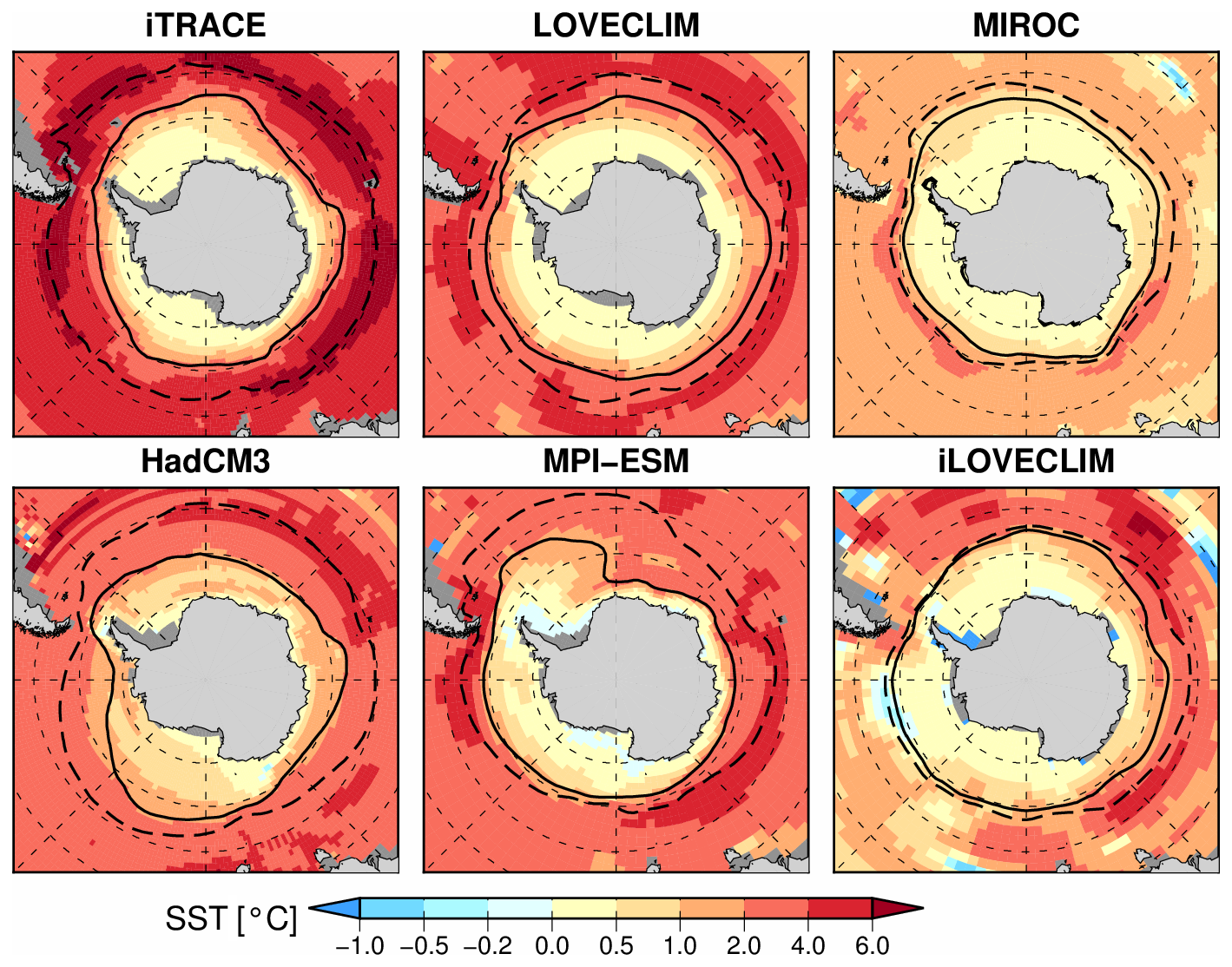
Figure 5 SST anomalies at 11 ka compared to the LGM. The bold and dashed lines indicate LGM and 11 ka sea ice extent (15 % sea ice concentration), respectively.

The different magnitudes of simulated warming during Heinrich Stadial 1 and the Younger Dryas across the models could be explained by the range of LGM temperature changes with respect to the pre-industrial period, as the mean SAT and SST changes are different by a factor of 2 (Table 1). To reduce this model difference, Antarctic SATs are normalized by the temperature anomaly between LGM and the pre-industrial period in Fig. 6. When normalized, the simulations with a weak AMOC during Heinrich Stadial 1 show the largest warming over Antarctica (Fig. 6, left column). The normalized Antarctic SAT change at 11 ka lies between 0.6 and 0.8 times the total temperature change between the LGM and pre-industrial period for five out of six models, indicating additional warming is simulated between 11 and 0 ka in the model simulations. This is different from ice core reconstructions for which the temperature at 11 ka is inferred to be comparable to the pre-industrial values (Parrenin et al., 2013; Buizert et al., 2021).

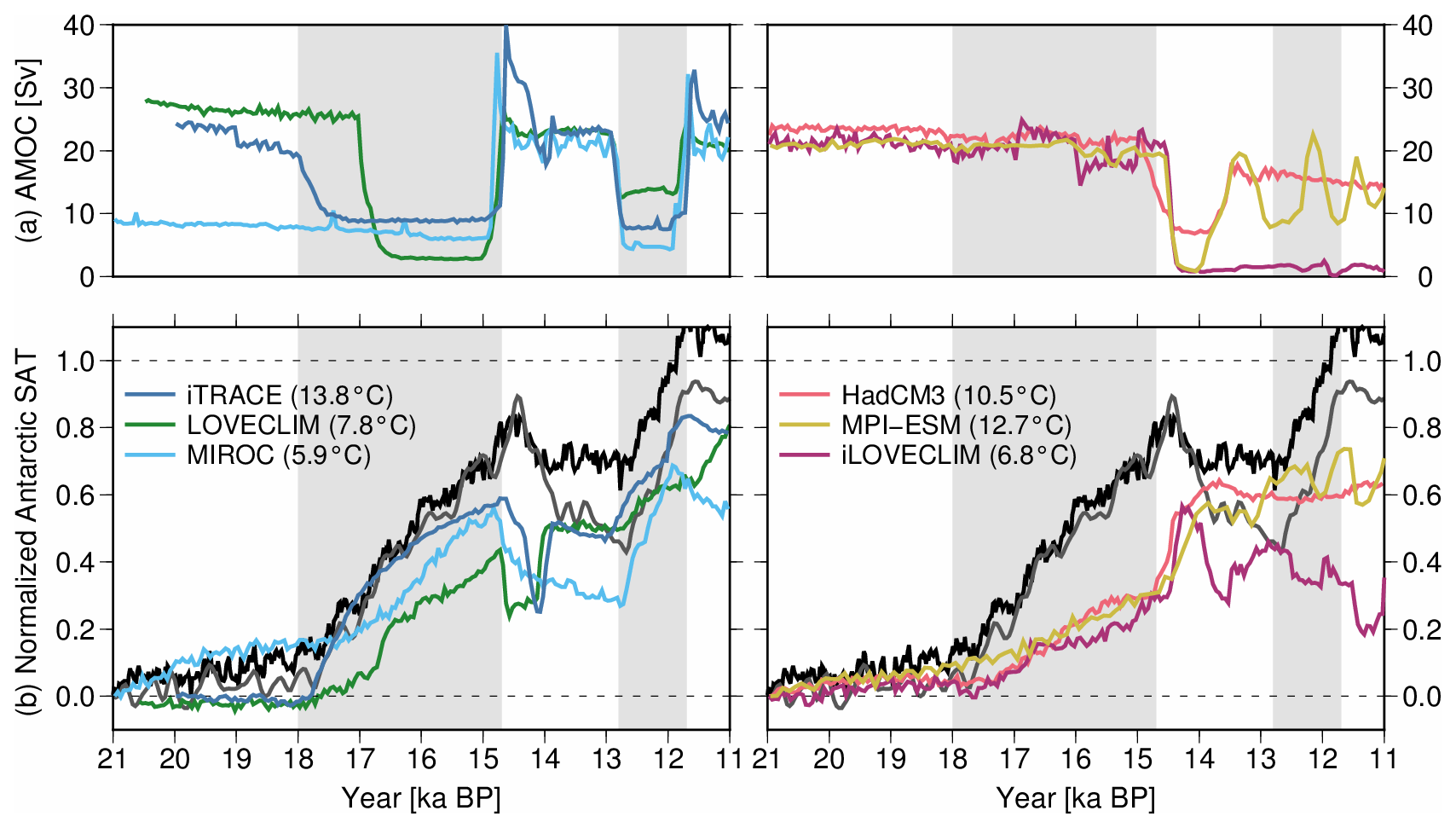
Figure 6 AMOC and normalized Antarctic SAT, with respect to the difference between the pre-industrial period and LGM. The actual pre-industrial and LGM differences are indicated in parentheses. The left panels show three simulations with weak AMOC during Heinrich Stadial 1, and the right panels show strong AMOC during Heinrich Stadial 1. The grey and black lines in panel (b) are normalized Antarctic SAT recorded by EDC ice based on Parrenin et al. (2013) and Buizert et al. (2021), respectively. The vertical grey shading from left to right indicates Heinrich Stadial 1 (18–14.7 ka) and the Younger Dryas (12.8–11.7 ka), and the period in between corresponds to the Bølling–Allerød (14.7–12.8 ka).

3.2 SST–CO₂–AMOC relationship analysis

The simulated AMOC time series display large differences across simulations due to different freshwater forcing groups, which complicates the quantification of CO₂ forcing and AMOC changes in driving high-southern-latitude temperature changes in each model. To overcome this, we examine the Southern Ocean SST trajectory against CO₂ forcing and AMOC strength (Fig. 7). Figure 7 shows that the deglacial increase in atmospheric CO₂ has major impacts on the Southern Ocean SST because the temperature trajectory is mostly proportional to CO₂ changes unless there are major AMOC changes. Temperature changes associated with changes in AMOC are superimposed on Southern Ocean SSTs; when AMOC is weak compared to the long-term mean of the respective models (blue circles), this tends to induce warming, and vice versa. Even though the actual time series of maximum AMOC strength in each model is very different, this result suggests that high-southern-latitude temperature changes can be decomposed into the effects of CO₂ and AMOC. The relative importance of CO₂ and AMOC are quantified in the following subsections.

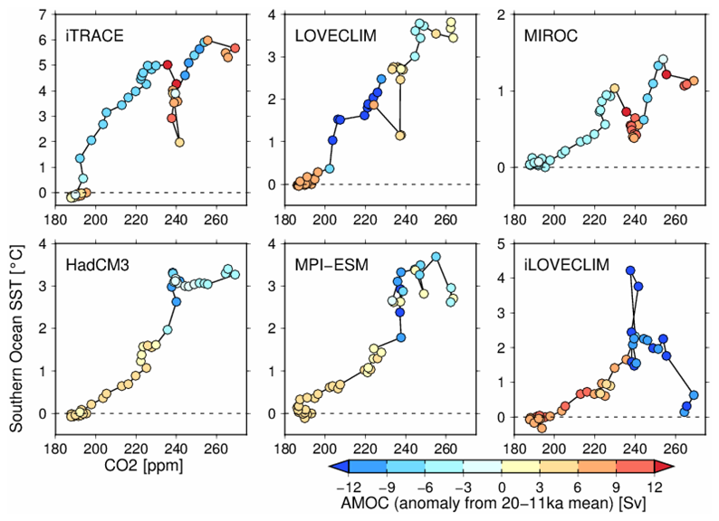
Figure 7 Relationship between Southern Ocean SST (vertical axis, change since LGM), CO₂ (horizontal axis), and AMOC strength anomaly from the mean strength between 20–11 ka (colours). The trajectory of the deglacial CO₂ forcing (CO₂), simulated SST changes, and AMOC are plotted with circles at 200-year intervals. Note that the vertical axes are different between models to represent the total deglacial warming.

3.3 Results of MLR and bipolar seesaw model

The results of the MLR model indicate that the CO₂ coefficients range from 1.0 to 6.5 °C for the total deglacial CO₂ changes (Table 3). All models have a negative coefficient of AMOC (−0.3 to −2.4 °C), indicating a Southern Ocean SST increase associated with AMOC weakening. The regression against Southern Ocean 2-D SST fields indicates that the CO₂ coefficient is mostly positive over the Southern Ocean, ranging from ∼ 0.5 °C in the Antarctic zone where sea ice is present until 11 ka to 2–6 °C in the Southern Ocean north of the LGM winter sea ice edge (Fig. 8). The sensitivity to the AMOC is mostly negative in the Southern Ocean, and areas of high sensitivity overlap with those of CO₂, suggesting sea ice modulates the areas sensitive to both CO₂ and AMOC changes.

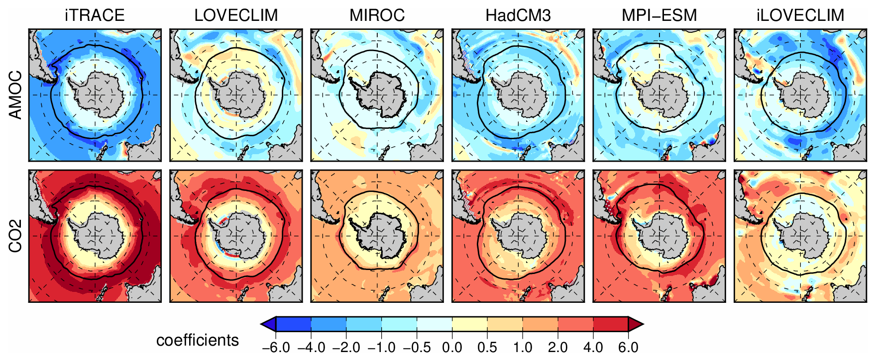
Figure 8 Results of the MLR model for 2-D SST maps. Top and bottom panels indicate AMOC [K per normalized AMOC] and CO₂ coefficients [K per 83 ppm]. The black lines represent LGM winter sea ice edges.

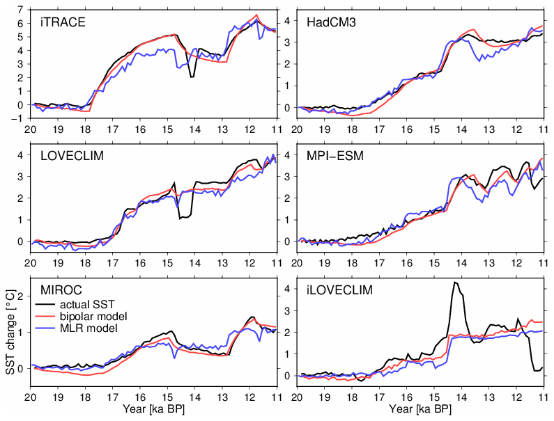
Figure 9 Results of the MLR model and bipolar seesaw model for Southern Ocean SST. The black lines represent the actual SST change (anomaly from 20 ka). The blue and red lines represent the results of MLR and bipolar seesaw models, respectively.

Table 5 summarizes the results of the bipolar seesaw model. All models have positive CO₂ coefficients (2.0 to 6.0 °C) and negative AMOC coefficients (−0.5 to −2.9 °C), as in the MLR models. The time series simulated by the bipolar seesaw model are compared with actual SST changes and with MLR models in Fig. 9. The bipolar seesaw model succeeds in reproducing a gradual SST decrease as a result of an AMOC strengthening (e.g. gradual cooling in iTRACE and MIROC, 15–13 ka). This gradual cooling was not represented by the MLR model, which exhibits an immediate SST response to AMOC changes. With the bipolar seesaw model, the response time ranges from 100–700 years, with most models ranging from 500–700 years with the exception of LOVECLIM and iLOVECLIM (Table 5). We also fed the bipolar seesaw model with the AMOC and CO₂ coefficients from six different models (Table 5) but with the common inputs of CO₂ (Bereiter et al., 2015) and AMOC from iTRACE. The results indicate that all models would have simulated a cooling at the surface of the Southern Ocean during the Bølling–Allerød if there was an increase in the AMOC at the beginning of the Bølling–Allerød as simulated in iTRACE, LOVECLIM, or MIROC (Fig. S2).

We note that the values of the CO₂ sensitivity from the MLR and bipolar seesaw model may include gradual forcing from other greenhouse gases, ice sheets, and orbital forcing. In addition, a sharp cooling associated with freshwater in the Antarctic Ocean was not represented because both models, MLR and bipolar seesaw, do not consider meltwater in the Southern Hemisphere (∼ 14.5 ka of iTRACE and LOVECLIM, ∼ 11.5 ka of MPI-ESM and iLOVECLIM)

3.4 Other Southern Ocean climate variables

We further analyse Antarctic Bottom Water transport (defined as the minimum global meridional overturning streamfunction, at depths below 3000 m and between 60 and 30​​​​​​​° S) as an indicator of Southern Ocean meridional circulation and 850 hPa zonal mean winds over the Southern Ocean (zonal mean winds averaged over 65–40° S) to analyse the potential impact on deglacial CO₂ changes, which is prescribed in the experiments. We focus on the onset of deglaciation (21–18 ka) and the initial significant increase in CO₂ (during Heinrich Stadial 1, 18–15 ka). Antarctic Bottom Water (Fig. 10b) at the LGM ranges from 10 to 30 Sv among the six models and stays relatively constant between 21 and 18 ka. In the subsequent period (18–15 ka), iTRACE exhibits a gradual decline in Antarctic Bottom Water, in phase with Southern Ocean SST changes (Fig. 10d). LOVECLIM and MPI-ESM exhibit a gradual decline in Antarctic Bottom Water (∼ 5 Sv), while three other models (MIROC, HadCM3, iLOVECLIM) exhibit a small reduction in or constant Antarctic Bottom Water formation. Thus, while all models simulate Southern Ocean SST warming and sea ice retreat during Heinrich Stadial 1, the trends in Antarctic Bottom Water formation differ. In addition, the Antarctic Bottom Water changes do not depend on the AMOC evolution and thus freshwater forcing groups (Fig. 10a–b). The zonal winds over the Southern Ocean exhibit slight change between 21 and 18 ka, apart from MIROC and MPI-ESM, which both exhibit a slight weakening (Fig. 10c). Between 18 and 15 ka, the zonal winds continue to decline in MIROC and MPI-ESM and start to decline in iTRACE and LOVECLIM. Little changes in zonal winds are simulated in iLOVECLIM, while HadCM3 exhibits a ∼ 10 % strengthening.

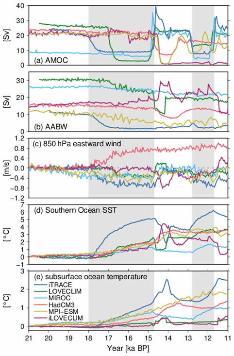
Figure 10 Time series of simulated (a) AMOC, (b) Antarctic Bottom Water, (c) 850 hPa eastward winds over the Southern Ocean (65–40° S), (d) Southern Ocean SST, and (e) subsurface ocean temperature south of 60° S (at depths 400–666 m). The vertical grey shading from left to right indicates Heinrich Stadial 1 (18–14.7 ka) and the Younger Dryas (12.8–11.7 ka), and the period in between corresponds to the Bølling–Allerød (14.7–12.8 ka).

Subsurface ocean temperatures south of 60° S at depths of around 500 m (Fig. 10e) exhibit an increase during Heinrich Stadial 1 in 4 of the 6 simulations, with the largest warming (1.2 and 0.8 °C) simulated by the two simulations which exhibited the largest SST increase (iTRACE and MPI-ESM). During the Bølling–Allerød (15–13 ka), iTRACE and MIROC exhibit a gradual subsurface temperature decrease, while HadCM3 and MPI-ESM exhibit continuous warming, as per the SST changes in the respective models. iLOVECLIM and LOVECLIM exhibit small changes (< 0.5 °C) in the total subsurface temperature. Abrupt subsurface warming in iTRACE (∼ 14 ka) and LOVECLIM (14.8–14.2 ka) coincide with Southern Ocean SST reduction, suggesting that this results from enhanced Southern Ocean stratification as a response to Southern Ocean meltwater input (Menviel et al., 2011; Lowry et al., 2019).

3.5 Additional freshwater experiments on Heinrich Stadial 1 Southern Ocean warming in MIROC and HadCM3

We additionally show two simulations run with the MIROC and HadCM3 models to assess the impact of freshwater forcing on high-southern-latitude climate during Heinrich Stadial 1. As a reminder, MIROC and HadCM3 are assigned to different freshwater groups (Fig. 2). In the MIROC simulations, the freshwater forcing during Heinrich Stadial 1 is increased to 0.1 or 0.2 Sv between 18 and 15.5 ka (Fig. 11a, red and orange lines) instead of 0.03 Sv in the standard simulation. This larger meltwater input further weakens the AMOC (Fig. 11a) and leads to an additional 1 °C SST increase in the Southern Ocean compared to the standard simulation (Fig. 11d). The 1 °C warming in response to the AMOC reduction of ∼ 5 Sv is a greater response than is produced by the MLR and bipolar seesaw models. In the HadCM3 simulations, a North Atlantic freshwater flux of ∼ 0.2 Sv during Heinrich Stadial 1 (similar to Trace-21ka DGL-A; Liu et al., 2009) reduces the AMOC by 15 Sv (Fig. 11e blue lines) and induces an additional ∼ 1 °C increase in Southern Ocean SST compared to the standard simulation (Fig. 11h). The simulated Heinrich Stadial 1 warming in HadCM3 is consistent with both MLR and bipolar seesaw models (Tables 3 and 5). The results from the MIROC and HadCM3 sensitivity experiments show that the simulated warming during Heinrich Stadial 1 can be twice as strong with an AMOC shutdown compared to the standard simulation of each model. As in the LOVECLIM Heinrich Stadial 4 simulation (Fig. S2; Margari et al., 2020), high-southern-latitude temperatures do not necessarily respond linearly to changes in AMOC strength, and MLR models assume a linear temperature response to the AMOC.

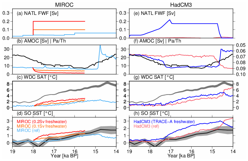
Figure 11 Results from transient deglaciation experiments performed with (a–d) MIROC and (e–h) HadCM3. The black lines in each panel represent the same proxy data as in Fig. 3 (Parrenin et al., 2013; Buizert et al., 2021; Anderson et al., 2020). In two MIROC sensitivity experiments, a larger amount of freshwater flux (0.1 or 0.2 Sv) is added into the North Atlantic (50–70° N) during 18–15.5 ka compared to the standard MIROC experiment (light blue lines). In the TRACE-A HadCM3 sensitivity experiment (blue lines), a larger freshwater flux is added in the North Atlantic following the Trace-21ka simulation (Liu et al., 2009), while the pink lines in panel (b) represent the HadCM3 simulation used by Snoll et al. (2022).

4 Discussion

4.1 Onset of deglacial warming

The climate forcing in the early deglaciation primarily comes from insolation due to obliquity and precession changes (Fig. 1a), which leads to an increase in spring to summer insolation south of 60 ° S (Fig. S3). Ice core data suggest that the onset of deglacial warming at WDC was earlier than the increase in CO₂, and this early deglacial warming has been suggested to result from an AMOC reduction (Shakun et al., 2012) or local insolation changes (WAIS Divide Project Members, 2013). However, simulated early warming is smaller than inferred from proxy records. Three models (MIROC, HadCM3, MPI-ESM) exhibit a small warming (∼ 0.5 °C) between 21 and 18 ka (Fig. 4a) in both West and East Antarctica, as well as at the surface of the Southern Ocean, primarily in the Pacific sector (Fig. 4b), consistent with proxy records (Moy et al., 2019; Sikes et al., 2019; Moros et al., 2021) and a previous modelling study (Timmermann et al., 2009). The other models show a slight cooling (iTRACE) or little change (LOVECLIM and iLOVECLIM).

The first explanation for the differences in the simulated temperature change between 21 and 18 ka relates to Southern Ocean sea ice at the LGM. MIROC, HadCM3, and MPI-ESM have less LGM summer sea ice than other models, which may lead to a relatively high sensitivity to increased insolation during austral spring to summer, causing significant warming with sea ice retreat (Timmermann et al., 2009; Roche et al., 2011). If the LGM Southern Ocean sea ice extent is extensive, the increase in insolation primarily south of 60° S (Fig. S3) does not warm the Southern Ocean as much because of high sea ice albedo. Although the local insolation changes are the likely cause of the early warming simulated in some of the models, the addition of freshwater could contribute to the AMOC weakening. For example, the consideration of an additional freshwater flux from the Fennoscandian ice sheet in the freshwater forcing prior to 18 ka, suggested by Toucanne et al. (2010), would weaken the AMOC and lead to a more pronounced warming at the high southern latitudes.

Another model–data difference is in the early warming rates between West and East Antarctica. The data from WDC suggest there was significant warming in West Antarctica, while a less significant change in East Antarctica is suggested by EDC records. In contrast, the models simulate similar warming rates in both West and East Antarctica (Fig. 4a), suggesting the models may underestimate the spatial heterogeneity in West and East Antarctic warming. This might be attributed to the Antarctic ice sheet history prescribed in the experiments, where both ICE-6G_C and GLAC-1D have minor surface elevation changes at WDC in the early deglaciation (Fig. 1d). Buizert et al. (2021) used the MIROC and HadCM3 models to show that the uncertainty in Antarctic ice sheet height affects SAT due to the impact of lapse rates (∼ 1 °C warming per 100 m altitude reduction). This might suggest that the lower surface elevations at WDC, related to ice sheet terminus retreat from 20–15 ka in the Amundsen Sea (Bentley et al., 2014), contributed to the early deglacial warming primarily in West Antarctica. The coarse resolution of the atmospheric models (2.5 to 5.6° horizontally) may impact the warming contrast between East Antarctica (EDC ice core site) and West Antarctica (WDC ice core site) through an inherent smoothing of the surface topography of the Antarctic ice sheet and the associated impact on the atmospheric circulation (Buizert et al., 2021). In addition, the relatively coarse resolution of the ocean models (1 to 3°) may impact AMOC sensitivity to iceberg and freshwater fluxes in the North Atlantic (Condron and Winsor 2012) or mesoscale processes in the Southern Ocean (Morrison and Hogg, 2013) and their response to the deglaciation.

Uncertainty in Antarctic ice sheet topography could also explain some model–proxy record differences during the early Holocene, where simulations indicate that an additional warming occurs after 11 ka (Fig. 6). This is different from ice core data (Fig. 4) and global mean ocean temperature (including deep-sea temperature) estimated from noble gases in ice cores, which suggests that temperatures reach Holocene levels at the end of Younger Dryas (Bereiter et al., 2018). The decrease in surface elevation of the Antarctic ice sheet after 11 ka (Fig. 1e) may contribute to the Holocene warming. It would be valuable to assess the uncertainties from ice sheet reconstructions, as new reconstructions have been published (e.g. Gowan et al., 2021), and different LGM ice sheets can induce different AMOC variabilities (Prange et al., 2023; Masoum et al., 2024).

4.2 Rate of temperature changes

Heinrich Stadial 1 (∼ 18–14.7 ka) exhibits major warming in all models because of the CO₂ increase, with the total warming being dependent on the sensitivity of each model to CO₂ and to AMOC changes. In turn, the deglacial AMOC evolution is dictated by the glacial meltwater input, as shown in additional sensitivity experiments performed with MIROC and HadCM3 (Fig. 11). Among the six models, iTRACE simulates the largest warming during Heinrich Stadial 1, with an Antarctic SAT increase of 6–8 °C and a rise in Southern Ocean SST of 4–5 °C. While Antarctic SAT matches ice core data, simulated Southern Ocean SST is larger than the SST stack (Fig. 3e). Five models besides iTRACE simulate a Southern Ocean SST change that compares well with the SST stack, but these five models underestimate Antarctic SAT. This indicates that the different magnitudes of warming between Southern Ocean SST and Antarctic SAT are not fully reconciled in the physics-based models. While iTRACE exhibits the largest cooling of global mean SAT at the LGM compared to the pre-industrial period (7.3 °C, compared to the six-model mean of 5.3 °C), the ECS of iTRACE (3.6 °C) is not the highest among the six models; instead, MIROC4m has the highest ECS despite weaker deglacial warming (Table 1). We examine the relationship between ECS and the LGM global mean SAT changes using multi-model PMIP3 and PMIP4 simulations (Fig. S4). We find a weak negative correlation (−0.06) between the ECS and global mean LGM SAT changes, and the local SAT change in the individual climate models can vary by about a factor of 2 even with the same ECS. A substantial asymmetry between warm and cold climates has been identified in previous studies because of the presence of continental ice sheets, ocean dynamics, and cloud feedback (Yoshimori et al., 2009; Zhu and Poulsen, 2021). Hence, understanding the mechanisms and amplitude of cooling in the LGM simulations will contribute to a better understanding of multi-model differences in the deglacial warming.

The sensitivity to AMOC ranges between −0.5 and −2.9 °C based on the analysis using the thermal bipolar seesaw model (Table 5). A multi-model study comparing freshwater hosing experiments of 11 climate models (including LOVECLIM, MIROC, and HadCM3 used in this study) under LGM climate shows that most models exhibit warming in the Southern Ocean (Kageyama et al., 2013). However, the simulation length in that study is less than 420 years. In this study, we estimated that the bipolar seesaw operates on a timescale of ∼ 500–700 years. Thus, longer simulations are needed to evaluate the extent of the climate response at high southern latitudes.

The MLR and thermal bipolar seesaw models in this study include several assumptions. Firstly, as the gradual forcing is represented only by the CO₂ concentration, they do not consider the effect from retreating ice sheets, meltwater flux in the Southern Ocean, or insolation changes explicitly. Other forcings could be included in the CO₂ or AMOC coefficients in this analysis. For instance, insolation change in boreal summer is positively correlated with CO₂; both exhibit a gradual increase (Fig. 1a–b). Antarctic and Northern Hemisphere ice sheet changes could impact Southern Ocean SST (Abe-Ouchi et al., 2015). This may explain the CO₂ coefficients from the MLR and bipolar seesaw model being higher than expected from the ECS value. On the other hand, the AMOC sensitivity of the LOVECLIM model is low compared to the 1.5 °C Southern Ocean SST increase found in the simulation of Heinrich Stadial 4 (Margari et al., 2020; Fig. S5), and the CO₂ coefficient is quite high, potentially implying a poor separation or substantial interconnectivity of the two factors.

4.3 Freshwater forcing and temperature changes at high southern latitudes

As shown here, the deglacial AMOC variations are quite different amongst the simulations. Only those that display an AMOC increase at the end of Heinrich Stadial 1 can capture a cooling trend at the Bølling–Allerød (corresponding to the Antarctic Cold Reversal) consistent with ice core data (iTRACE, LOVECLIM, MIROC). In comparison to previous transient simulations of the last deglaciation, the representation of the duration of the Antarctic Cold Reversal has improved, as it was previously simulated as being too short (Lowry et al., 2019). On the other hand, individual climate model simulations that are forced with a large Northern Hemisphere meltwater pulse consistent with ice sheet reconstructions do not simulate an increase in the AMOC at the Bølling–Allerød (Ivanovic et al., 2016, 2018; Kapsch et al., 2022; Bouttes et al., 2023; Snoll et al., 2024). Freshwater forcing in the Northern Hemisphere and associated reduction in the AMOC led to Antarctic warming during Heinrich Stadial 1 in sensitivity experiments with individual forcing (He et al., 2013) and sensitivity experiments with freshwater forcing (Fig. 11).

A comparison of the six models reveals that capturing phase changes in the AMOC is necessary to simulate warming or cooling trends at high southern latitudes. This is also supported by results from the bipolar seesaw model simulations forced with a common AMOC (Fig. S2). While MIROC simulates a rapid increase in the AMOC at the Bølling–Allerød transition with a continuous freshwater flux (Fig. 2), a 50 % greater (i.e. 1.5 ×) freshwater forcing produces a weak AMOC throughout the last deglaciation (Obase et al., 2021). Thus, the simulated temperature changes at high southern latitudes are sensitive to freshwater forcing in the Northern Hemisphere.

However, the timing and magnitude of meltwater input inferred from ice sheet reconstructions conflict with the meltwater forcing needed to obtain a deglacial climate evolution in agreement with proxy records. This so-called meltwater paradox (Ivanovic et al., 2018; Snoll et al., 2024) is present for major periods of the last deglaciation including the Bølling–Allerød transition and Heinrich Stadial 1. This highlights a need for more accurately constrained freshwater forcing scenarios (and then envelope of uncertainty) and a need to assess the sensitivity of climate models to freshwater forcing (including the reduction in climate model biases impeding the correct sensitivity). We also note that the routing location of meltwater input (Roche et al., 2010; He et al., 2020) and the method for implementing iceberg and meltwater discharges into the ocean (Schloesser et al., 2019; Love et al., 2021) may induce different AMOC changes.

In addition, freshwater forcing from the Antarctic ice sheet can enhance the Antarctic Cold Reversal, as found in iTRACE (∼ 14.2 ka) and LOVECLIM (∼ 14.7 ka), with a sharp cooling in Southern Ocean SST and Antarctic SAT primarily in WDC. This is caused by the intensified stratification in the Southern Ocean (Menviel et al., 2010, 2011), which induces significant warming in the subsurface and contributes to further Antarctic ice mass loss (Golledge et al., 2014). As ice core data do not exhibit such sharp cooling events compared to climate model simulations (Fig. 3), this may provide some constraints on the extent and duration of freshwater forcing from the Antarctic ice sheet.

4.4 Implications for climate system changes at high southern latitudes

Reconstructions have suggested that changes in Southern Ocean circulation, probably driven by wind changes, were important for the modulation of Southern Ocean CO₂ outgassing during the deglaciation. Proxy records suggest there was an enhanced opal flux during Heinrich Stadial 1, which could reflect increased upwelling in the Southern Ocean due to changes in Southern Hemisphere westerlies (Anderson et al., 2009) and a poleward shift in the Southern Hemisphere Westerlies across the deglaciation (Gray et al., 2023). Proxies also suggest an increase in deep and intermediate-depth Southern Ocean ventilation (Skinner et al., 2010; Burke and Robinson, 2011), increasing intermediate-depth pH in the Southern Ocean during Heinrich Stadial 1 (Rae et al., 2018). It has been suggested that stronger or poleward-shifted Southern Hemisphere Westerlies and/or enhanced Antarctic Bottom Water formation during Heinrich Stadial 1 would indeed enhance Southern Ocean CO₂ outgassing and lead to an atmospheric CO₂ increase (Menviel et al., 2014, 2018).

In contrast, in the present study, most models show very little change or a gradual weakening in the Southern Hemisphere Westerlies throughout the deglaciation and there is little latitudinal migration. Only HadCM3 simulates a strengthening in the Westerlies during Heinrich Stadial 1. This relative inertia in the wind conditions may be influenced by biases in the Southern Hemisphere Westerlies in pre-industrial simulations. Additional research could study in more detail the changes in regional strength and their relation to other climatic variables (Rojas et al., 2009; Sime et al., 2013).

In addition, no model exhibits an increase in Antarctic Bottom Water formation, which could contribute to the upwelling of carbon-rich waters and CO₂ outgassing from the Southern Ocean. Instead, the long-term Antarctic Bottom Water weakening driven by Southern Ocean warming and sea ice melt is consistent with previous analyses of deglaciation experiments (Marson et al., 2016). While it has been suggested that larger Southern Ocean sea ice extent would lead to an atmospheric CO₂ decrease at the LGM (Ferrari et al., 2014; Marzocchi and Jansen, 2019; Stein et al., 2020; Kobayashi et al., 2021), few models simulate significant changes in atmospheric CO₂ due to Southern Ocean sea ice change (Gottschalk et al., 2019). These physical changes still need to be reconciled with processes put forward to explain the deglacial trends in atmospheric CO₂, for example, by running coupled climate–carbon simulations.

Finally, we also find that changes in subsurface ocean temperature in the Southern Ocean, one of the critical factors impacting the retreat of the Antarctic ice sheet, display significant differences across the simulations. This could be related to different ECS or freshwater forcing in the Southern Ocean and should also be investigated in future work to quantify uncertainties in subsurface ocean temperature changes. Model-dependent subsurface ocean temperature change is one source of uncertainty in projecting future Antarctic ice sheet mass loss (Seroussi et al., 2020). In contrast to the present simulations of the last deglaciation, which prescribe the Antarctic ice sheet history, climate variability occurring during the deglaciation can impact the Antarctic ice sheet, which can act as feedback to Southern Ocean climate via meltwater input from the Antarctic ice sheet (Menviel et al., 2010; Golledge et al., 2014; Clark et al., 2020). Hence, further coupled climate and ice sheet modelling studies are needed to improve our understanding of climatological and glaciological processes and to evaluate model performance under a warming climate and rising sea levels (Gomez et al., 2020).

5 Conclusion

In our multi-model analysis of transient deglacial experiments, the early increase in Antarctic SAT is weakly simulated or absent. The multi-model difference could be related to divergence in LGM sea ice extent, which may affect model sensitivity to insolation change, or to a slight reduction in the AMOC in response to low levels of freshwater input from the Northern Hemisphere ice sheets.

In addition, the different warming rates between West and East Antarctica inferred from ice core records are not reproduced by the transient simulations. In all models, a major warming occurs at high southern latitudes between 18 and 15 ka in response to increased CO₂ concentration. The multi-model analysis and sensitivity experiments further suggest that the AMOC reduction during Heinrich Stadial 1, which is associated with increased freshwater flux in the North Atlantic, contributes to a larger warming at high southern latitudes, in agreement with high-southern-latitude proxy records, even though no simulation can reproduce both the amplitude of Southern Ocean SST and Antarctic SAT changes simultaneously. The bipolar seesaw model indicates that all models have a bipolar seesaw response and that an abrupt AMOC increase at the end of Heinrich Stadial 1 is necessary to simulate the high-southern-latitude cooling during the Bølling–Allerød (corresponding to the Antarctic Cold Reversal).

The simulations exhibit little change in winds over the Southern Ocean and meridional circulation in the Southern Ocean, raising questions about what processes could have contributed to enhanced CO₂ outgassing from the Southern Ocean. This indicates the necessity for future climate system modelling studies to quantify the sequence of deglacial climate changes and atmospheric CO₂ increase.