Simulated ocean oxygenation during the interglacials MIS 5e and MIS 9e

Recent studies investigating future warming scenarios have shown that the ocean oxygen content will continue to decrease over the coming century due to ocean warming and changes in oceanic circulation. However, significant uncertainties remain regarding the magnitude and patterns of future ocean deoxygenation. Here, we simulate ocean oxygenation with the ACCESS ESM1.5 model during two past interglacials that were warmer than the preindustrial (PI) climate, the Last Interglacial (Marine Isotope Stage (MIS) 5e, ∼ 129–115 ka) and MIS 9e (∼ 336–321 ka). While orbital parameters were similar during MIS 5e and MIS 9e, with lower precession, higher eccentricity, and higher obliquity than PI, greenhouse gas radiative forcing was highest during MIS 9e and lowest during MIS 5e. We find that the global ocean is overall less oxygenated in the MIS 5e and MIS 9e simulations compared to the PI control run and that oxygen concentrations are more sensitive to changes in the distribution of incoming solar radiation than to differences in greenhouse gas concentrations. Large regions in the Mediterranean Sea are hypoxic in the MIS 5e simulation, and to a lesser extent in the MIS 9e simulation, due to an intensification and expansion of the African monsoon, enhanced river runoff and resulting freshening of surface waters and stratification. Upwelling zones off the coast of North America and North Africa are weaker in both simulations compared to the preindustrial control run, leading to less primary productivity and export production. Antarctic Bottom Water is less oxygenated, while North Atlantic Deep Water and the North Pacific Ocean at intermediate depths are higher in oxygen content. All changes in oxygen concentrations are primarily caused by changes in ocean circulation and export production and secondarily by changes in temperature and solubility.

1 Introduction

The global ocean oxygen inventory has decreased by over 2 % since 1960, and the volume of anoxic waters has more than quadrupled over the same time period (Schmidtko et al., 2017; Levin, 2018). This decrease was caused by a decline in oxygen solubility due to higher ocean temperatures (Bopp et al., 2013), but changes in ocean circulation and biological consumption also contributed to the observed changes (Ito et al., 2017; Breitburg et al., 2018). Model simulations project that this decline will continue into the future, although the spatial patterns and magnitude are model-dependent and strongly influenced by the models' ocean diffusivity parameters (Duteil and Oschlies, 2011; Gnanadesikan et al., 2012; Bopp et al., 2013; Long et al., 2016; Bahl et al., 2019; Frölicher et al., 2020; Kwiatkowski et al., 2020; Chamberlain et al., 2024). Future ocean deoxygenation could eventually pose severe problems for ocean ecosystems and human societies (Diaz and Rosenberg, 2008; Vaquer-Sunyer and Duarte, 2008; Sampaio et al., 2021; Penn and Deutsch, 2022; Santana-Falcón et al., 2023), and there has been a growing interest in recent years to better quantify ocean deoxygenation and understand its drivers.

Ocean oxygenation has also changed in the past. For example, Scholz et al. (2014) find sulfidic conditions in the near-surface sediments of the Peruvian upwelling area during the Last Interglacial (LIG) period (Marine Isotope Stage (MIS) 5e, ∼ 129–116 kyr ago), based on sedimentary molybdenum accumulation. Records of sedimentary δ¹⁵N and redox-sensitive metals show that interglacials in the late Quaternary led to an expansion and/or intensification of near-surface and intermediate-depth suboxic zones in the eastern Pacific margins and the Arabian Sea compared to glacials (Ganeshram et al., 2000; Galbraith et al., 2004; Nameroff et al., 2004; Glock et al., 2022). These changes in oxygenation have been generally assigned to changes in oxygen supply to the global thermocline (Galbraith et al., 2004; Meissner et al., 2005; Muratli et al., 2010; Jaccard and Galbraith, 2012). For large regions of the deep ocean this trend was inverted (Hoogakker et al., 2018), and deep and bottom waters were better ventilated during interglacials compared to glacials. Jaccard et al. (2009) report close to suboxic conditions during glacial intervals of the past 150 kyr compared to better ventilated conditions during MIS 5e and the Holocene (the past 11 700 years) in the deep subarctic Pacific. In the deep equatorial Pacific there is multi-proxy evidence for reduced oxygen concentrations in all deep Pacific Ocean water masses below 1 km during glacials compared to MIS 5e and the Holocene (Anderson et al., 2019; Jacobel et al., 2020). Bottom waters in the northern Arabian Sea, on the Portuguese margin, and in the North and South Atlantic, as well as South Atlantic Circumpolar Deep Water (CDW), were also less oxygenated during glacial episodes compared to MIS 5e and the Holocene (den Dulk et al., 1998; Hoogakker et al., 2015, 2016; Lu et al., 2016; Gottschalk et al., 2020). It is noteworthy that most reconstructions of ocean oxygenation in the late Quaternary compare glacials with interglacials; there is very little evidence on how oxygen concentrations varied between interglacials. This is an important caveat, as better understanding of ocean oxygen variability in the past, and, in particular, ocean oxygenation during past warm episodes, could inform on the main processes influencing current ocean deoxygenation.

One region with notably large changes in past ocean oxygen concentrations is the semi-enclosed Mediterranean Sea, where there is evidence of intervals with severe anoxia during past interglacials (Sachs and Repeta, 1999; Rohling et al., 2015; Rush et al., 2019). These intervals are characterized by sediment layers with elevated organic carbon concentrations (sapropels) and coincide with astronomically timed episodes of monsoon intensification, causing enhanced runoff from North Africa into the Mediterranean Sea and leading to stratification (Rohling et al., 2015). The resulting anoxia was often more intensely developed in the eastern Mediterranean than in the western Mediterranean.

Here, we analyze simulations integrated with the Australian earth system model ACCESS-ESM1.5 for two interglacials, MIS 5e, or the Last Interglacial (LIG), and MIS 9e. The LIG is an interesting time period because it was globally the warmest interglacial of the past 800 kyr (Past Interglacials Working Group of PAGES, 2016). Being the most recent interglacial, the spatial and temporal resolution of climate proxies is also much better than for earlier interglacials. The LIG climate has been recently simulated by a variety of climate models under the Paleoclimate Model Intercomparison Project 4 (PMIP4) lig127k experiment (Otto-Bliesner et al., 2017, 2021).

MIS 9e (∼ 336–321 kyr ago) stands out by its high greenhouse gas forcing, with the highest carbon dioxide and methane concentrations over the past 800 kyr (Past Interglacials Working Group of PAGES, 2016). It is also one of the three interglacials (together with MIS 11 and MIS 17) with the lowest value of seawater δ¹⁸O, which might imply high sea levels and small continental ice volumes (Elderfield et al., 2012; Past Interglacials Working Group of PAGES, 2016), although sea-level records from the Red Sea show that MIS 5e had higher sea levels than MIS 9e (Rohling et al., 2009). MIS 9e was an exceptionally short interglacial with the warmest temperatures in Antarctica over the past 800 kyr (Past Interglacials Working Group of PAGES, 2016). We will focus on how changes in orbital parameters and greenhouse gas concentrations influenced simulated ocean oxygenation for these two interglacials.

This paper is structured as follows. Section 2 describes the model, the experimental setup, and the time series for each of the analyzed experiments. Section 3 first analyses changes in large-scale circulation patterns and oxygenation and then focuses on changes in the Mediterranean Sea. In Sect. 4 we discuss uncertainties and situate our results within a broader context. Section 5 summarizes the main results.

2 Methods

We use the Australian Community Climate and Earth System Simulator Earth System Model, ACCESS-ESM1.5 (Ziehn et al., 2020), to integrate three equilibrium simulations under preindustrial, MIS 5e, and MIS 9e boundary conditions. The model includes the atmosphere UK Met Office Unified Model (UM) version 7.3 (Martin et al., 2010; The HadGEM2 Development Team, 2011), the Community Atmosphere Biosphere Land Exchange model (CABLE) version 2.4 (Kowalczyk et al., 2013), the NOAA/GFDL Modular Ocean Model (MOM) version 5 (Griffies, 2014), and the Los Alamos National Laboratory sea ice model (LANL CICE) version 4.1 (Hunke et al., 2010). The components communicate with each other through the Ocean Atmosphere Sea Ice Soil Model Coupling Toolkit (OASIS-MCT; Craig et al., 2017). The land and atmosphere components have a horizontal resolution of 1.875° × 1.25°, with 38 vertical levels for the atmosphere model. The ocean and sea ice components have a resolution of 1° × 1°, with 50 vertical levels for the ocean model. The horizontal resolution of the ocean model is higher near the Equator (0.33°) and in the Southern Ocean (∼ 0.4° at 70° S). Ocean biogeochemistry is represented by the Whole Ocean Model of Biogeochemistry And Trophic-dynamics (WOMBAT; Oke et al., 2013).

WOMBAT is a nutrient–phytoplankton–zooplankton–detritus (NPZD) model (Oke et al., 2013; Law et al., 2017; Ziehn et al., 2020). It includes one functional type of phytoplankton and zooplankton. As prognostic tracers it simulates dissolved inorganic carbon (DIC), alkalinity (ALK), phosphate (PO₄), oxygen (O₂), and iron. The stoichiometry is fixed at a C : N : P : O₂ ratio of 106 : 16 : 1 : −172. CaCO₃ export from the photic zone is set at ∼ 8 % of the organic carbon export. Detrital decomposition is a function of temperature and is allowed to occur when oxygen is zero. Even though nitrification and denitrification are not explicitly included in the model and the global nitrogen budget is kept constant (Oke et al., 2013), this formulation emulates the effect of denitrification. The dissolution of CaCO₃ occurs at a constant rate. All organic and inorganic particles reaching the bottom are remineralized, given that ACCESS-ESM1.5 does not include burial of sediments.

The preindustrial 1850 equilibrium simulation (PI) is integrated following the CMIP6 protocol (Eyring et al., 2016) with the exception of using the CMIP5 solar constant (1365.65 W m⁻²). The MIS 5e simulation (LIG) is integrated following the PMIP4 protocol (Otto-Bliesner et al., 2017) with the solar constant of CMIP5-PMIP3 (1365.65 W m⁻²). Both PI and LIG simulations have been evaluated extensively in the recent literature (Ziehn et al., 2020; Otto-Bliesner et al., 2021; Kageyama et al., 2021; Yeung et al., 2021; Mackallah et al., 2022; Choudhury et al., 2022; Yeung et al., 2024).

Table 1 Experimental setup. LIG boundary conditions follow the PMIP4 protocol (Otto-Bliesner et al., 2017). MIS 9e boundary conditions are based on Berger (1978) for orbital parameters and peak concentrations for methane (Loulergue et al., 2008), carbon dioxide (Bereiter et al., 2015), and nitrous oxide (Schilt et al., 2010). Please note that the first 372 years of the LIG simulation have erroneous forcing and were integrated with PI greenhouse gas concentrations.

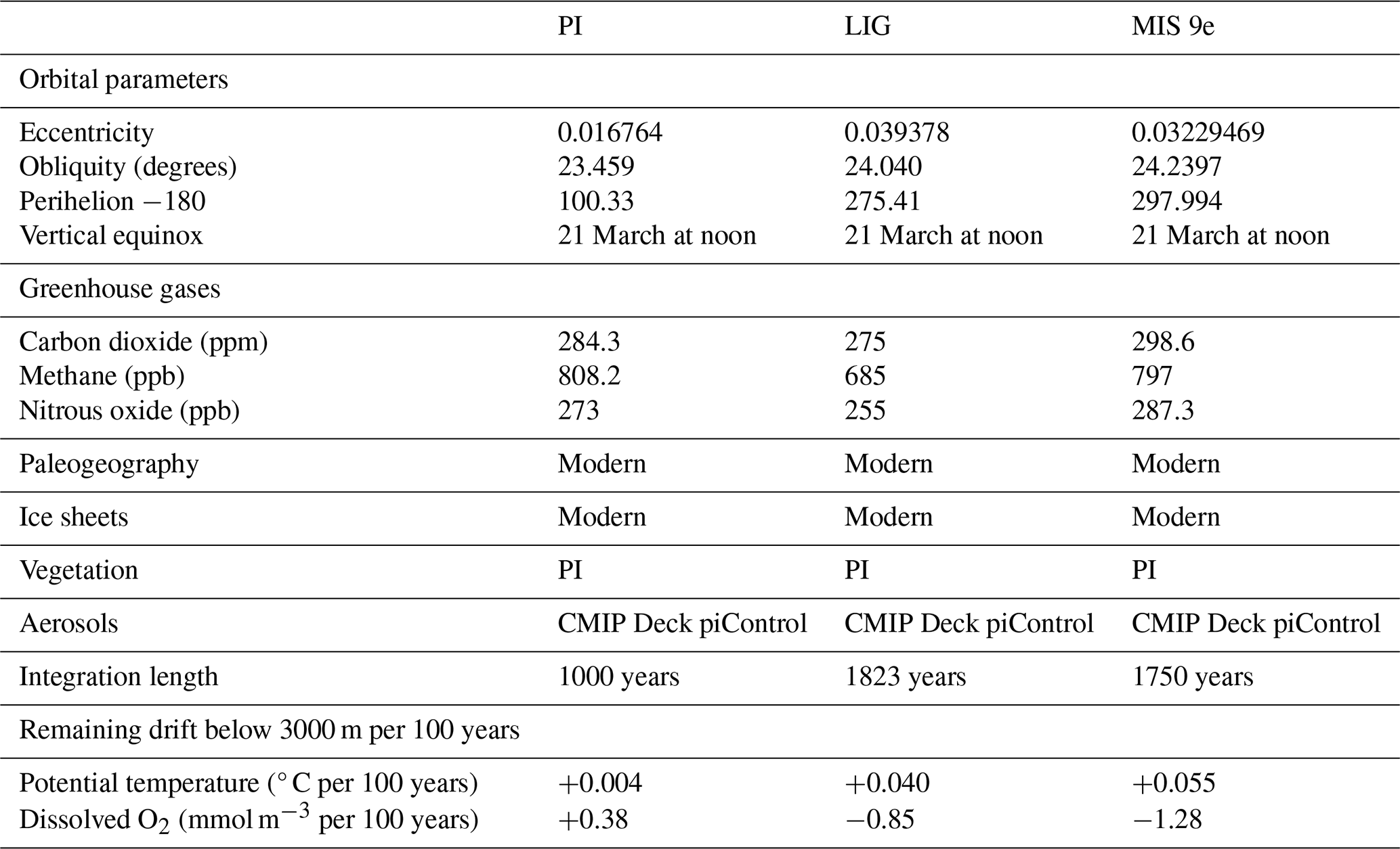
The MIS 9e simulation was set up with boundary conditions corresponding to 333 ka and the same solar constant as for PI and LIG (see Table 1). The Greenland and Antarctic ice sheets and vegetation distribution are the same in all three simulations, but the leaf area index is calculated prognostically. Anomalies in incoming solar radiation are shown in Fig. A1.

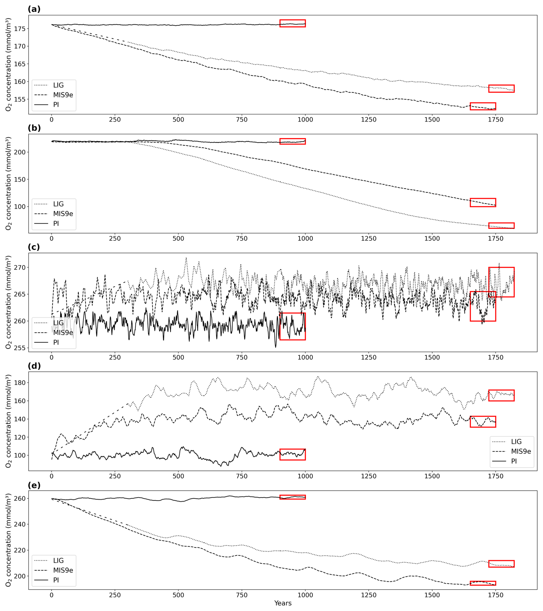
Figure 1 Time series of dissolved O₂ concentration in mmol m⁻³ averaged (a) globally, (b) in the Mediterranean Sea, (c) between 500 and 1200 m depth and 40–60° N (North Atlantic Deep Water), (d) between 250 and 1200 m depth and 40–60° N in the North Pacific, and (e) at 3000 m depth between 60 and 35° S (Antarctic Bottom Water) for PI (solid lines), LIG (dotted lines), and MIS 9e (dashed lines) simulations. Red rectangles designate the last 100 years of each simulation that are analyzed in this paper. The first 372 years of LIG were integrated with PI greenhouse gas concentrations and have been deleted from our file servers; we show therefore interpolations (long dashed lines) over this time span.

Dissolved oxygen is a tracer with very long equilibration times. Figure 1 shows time series of dissolved oxygen for the three simulations analyzed in this study. While oxygen concentrations have reached quasi-equilibrium for North Atlantic Deep Water (NADW), in the intermediate waters of the North Pacific, and in Antarctic Bottom Water (AABW) south of 35° S in all runs, there is still a slight drift in global mean dissolved oxygen in our LIG and MIS 9e simulations and a more substantial drift in the Mediterranean Sea.

In Sect. 3 we partition changes in dissolved oxygen into two components, changes in the saturated concentration of oxygen O${}_{\mathrm{2}}^{\mathrm{sat}}$ and changes in apparent oxygen utilization (AOU). AOU estimates the oxygen consumed during respiration and can be calculated as the difference between dissolved oxygen concentration (O₂) and O${}_{\mathrm{2}}^{\mathrm{sat}}$:

$$\begin{array}{}\text{(1)}& \mathrm{AOU}={\mathrm{O}}_{\mathrm{2}}^{\mathrm{sat}}(T,S)-{\mathrm{O}}_{\mathrm{2}},\end{array}$$

where T is the potential temperature and S salinity. Changes in AOU are therefore a combination of changes in circulation (with sluggish water masses tending to have higher AOU) and changes in remineralization rates, which depend on the vertical export of organic matter (export production) and temperature. Please note that the here used metric AOU assumes that dissolved oxygen in surface waters is in equilibrium with the atmosphere, which might lead to an overestimation of the true oxygen utilization (TOU) (Duteil et al., 2013).

3 Results

3.1 Large-scale oxygenation

All results reported in this section are based on 100-year means, calculated over the last 100 years of each simulation (see rectangles in Fig. 1). The global temperature patterns simulated by ACCESS ESM1.5 under LIG boundary conditions are described elsewhere (Otto-Bliesner et al., 2021; Yeung et al., 2021, 2024). Figure 2 shows annual-mean surface air temperature (SAT) anomalies and sea surface temperature (SST) anomalies for the simulations described in this study. Due to different orbital parameters, and in particular a positive summer insolation anomaly at high northern latitudes and a positive spring anomaly at high southern latitudes (Mitsui et al., 2022; Fig. A1), the annual-mean surface air temperature in our LIG simulation is 1.11 and 1.40 °C higher north and south of 40° N/S, respectively, compared to PI. While the insolation during MIS 9e is similar to LIG (Mitsui et al., 2022), greenhouse gas concentrations are higher (Table 1), with anomalies of ∼ 24 ppm for CO₂, ∼ 112 ppb for CH₄, and ∼ 32 ppb for N₂O, thus leading to globally warmer conditions in our MIS 9e simulation compared to the LIG simulation (Fig. 2). The annual-mean surface air temperature is 0.49 and 1.20 °C higher in the LIG and MIS 9e runs, respectively, compared to PI.

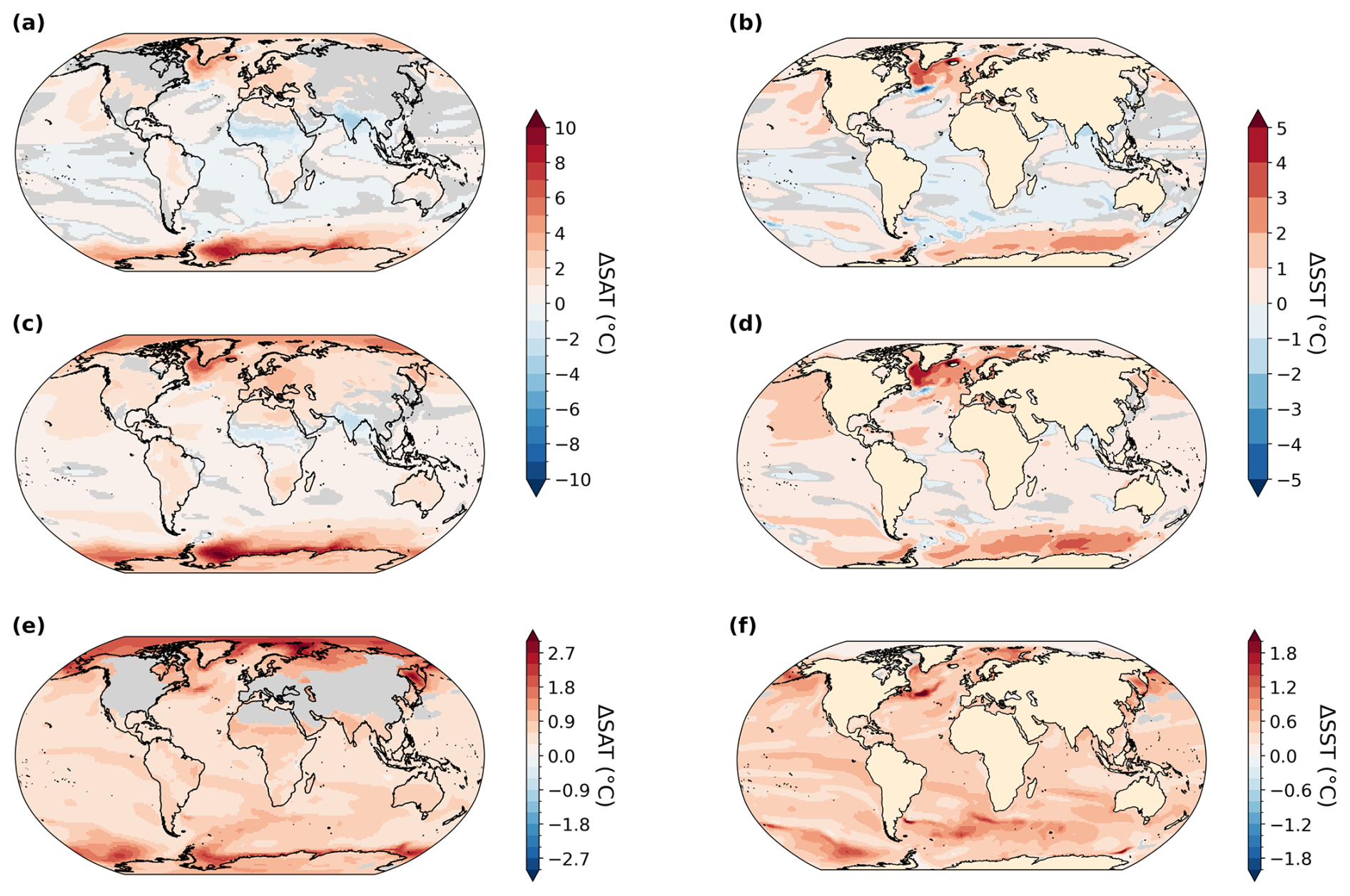
Figure 2 Annual-mean near-surface air temperature (SAT) anomalies (a, c, e) and sea surface temperature (SST) anomalies (b, d, f) in degrees Celsius (°C). Statistically insignificant differences (p value > 0.05) are shaded in gray. (a, b) LIG–PI, (c, d) MIS 9e–PI, (e, f) MIS 9e–LIG.

The PI simulation reproduces observed patterns of dissolved oxygen (World Ocean Atlas, 1965–2020) reasonably well (Ziehn et al., 2020; Fig. 3c and d) but underestimates O₂ in the eastern Pacific Ocean and southeastern Atlantic Ocean. It overestimates O₂ in the Arabian Sea, the Southern Ocean, and the Arctic. The global mean ocean O₂ concentration equals 176.3 mmol m⁻³ in our PI simulation compared to 158.0 and 154.5 mmol m⁻³ in the LIG and MIS 9e simulations, respectively. The largest differences between the simulations are located in the deep ocean (below 2500 m depth) and follow the pathways of Antarctic Bottom Water (AABW; Figs. 3 and 4). Overall, the anomalies in LIG and MIS 9e compared to PI are quite similar, with the loss in AABW O₂ being slightly less pronounced in LIG (Figs. 3 and 4). Significant differences can also be seen in the Mediterranean Sea (Fig. 3, Sect. 3.2).

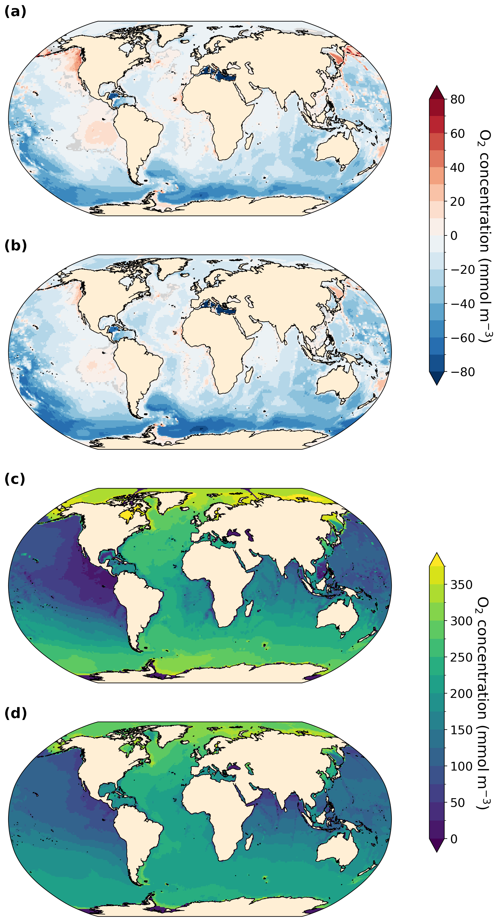
Figure 3 Vertically averaged dissolved O₂ concentration anomalies in mmol m⁻³. Statistically insignificant differences (p value > 0.01) are shaded in gray. (a) LIG–PI, (b) MIS 9e–PI, (c) vertically averaged dissolved O₂ concentration for the PI simulation, and (d) vertically averaged O₂ concentration from World Ocean Atlas (WOA, 1965–2022; Garcia et al., 2024).

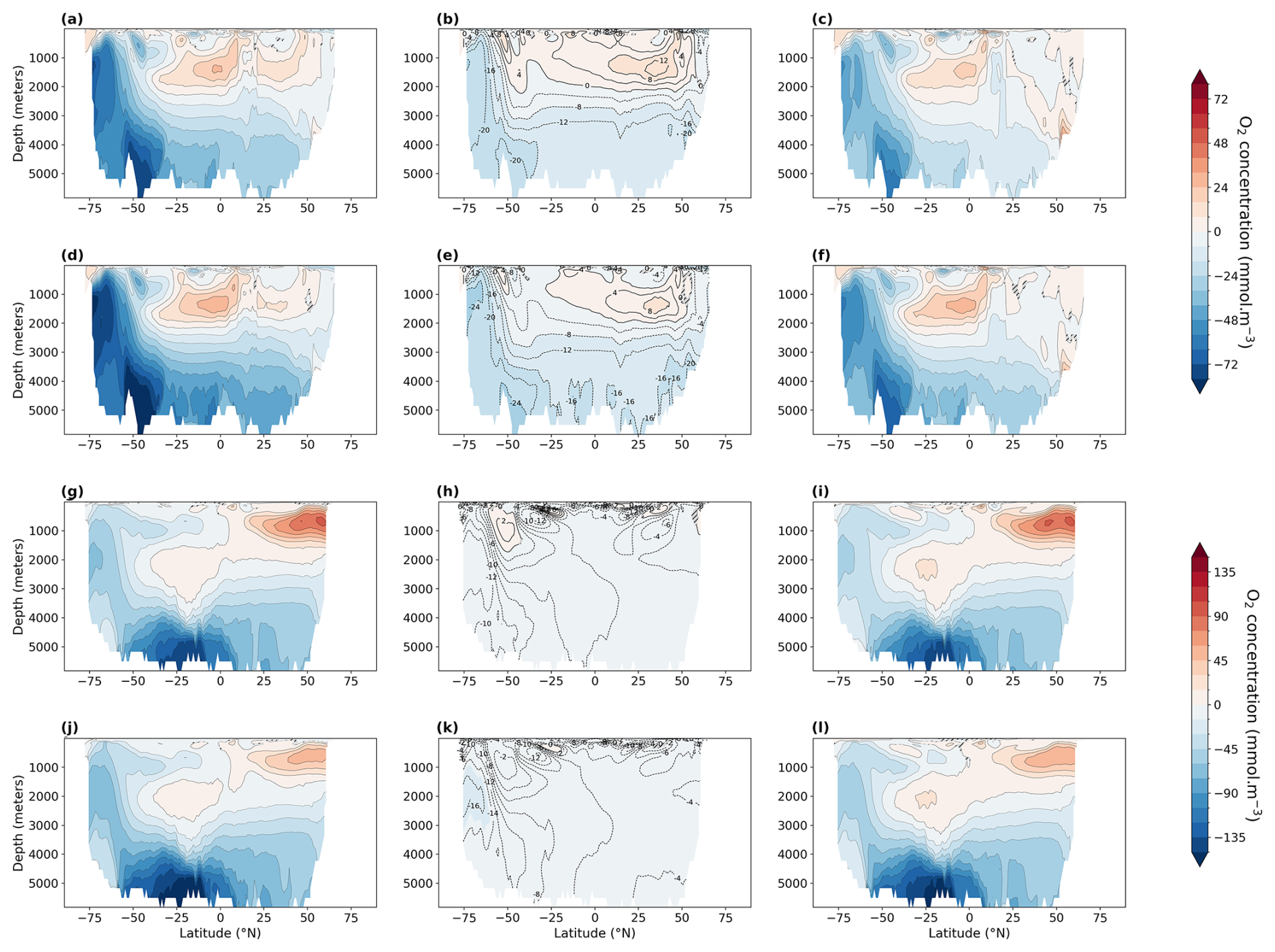
Figure 4 Zonally averaged dissolved O₂ concentration in mmol m⁻³ (left), saturated O₂ concentration (middle), and $-\mathrm{1}\cdot$AOU (apparent oxygen utilization, right). Statistically insignificant differences (p value > 0.01) are hatched and shaded in gray. Atlantic Ocean anomalies: LIG–PI (a–c) and MIS 9e–PI (d–f). Pacific Ocean anomalies: LIG–PI (g–i) and MIS 9e–PI (j–l). To facilitate the comparison between oxygen solubility and oxygen utilization, we multiplied AOU by −1.

The next two subsections analyze changes in the main large-scale bottom and deep water masses, AABW and NADW. We also see significant changes in the oxygenation of North Pacific Intermediate Water, which are described in Sect. 3.1.3. Changes in low-oxygen zones can have a large impact on marine life and biogeochemical cycles. We therefore analyze changes in the simulated oxygen minimum zones in Sect. 3.1.4.

3.1.1 Antarctic Bottom Water – warmer and less ventilated

AABW is warmer and weaker in our LIG and MIS 9e simulations compared to PI (Fig. A2). At 30° S, the maximum absolute value of the streamfunction reaches 3.8 Sv (sverdrups) in LIG and 2.9 Sv in MIS 9e compared to 7.9 Sv in PI (Fig. 5). Bottom water convection sites in the Weddell, Lazarev, and Ross seas are smaller in spatial extent and are also less intense (Fig. A3). This weakening of deep-ocean convection is mainly due to reduced sea ice formation (Yeung et al., 2024; Choudhury et al., 2022) and leads to warmer, less ventilated, and therefore less oxygenated AABW. The relative contribution of changes in apparent oxygen utilization (AOU) is higher than the contribution of changes in solubility (compare middle and right columns in Fig. 4). Export production is enhanced in the Southern Ocean in LIG and MIS 9e compared to PI (Choudhury et al., 2022; Fig. 6), and remineralization rates are higher due to higher temperatures (Choudhury et al., 2022). Changes in dissolved oxygen concentrations in AABW are therefore primarily due to the weakening of Antarctic Bottom Water circulation, together with the increase in export production and higher remineralization rates, and secondarily caused by the temperature-dependent solubility effect.

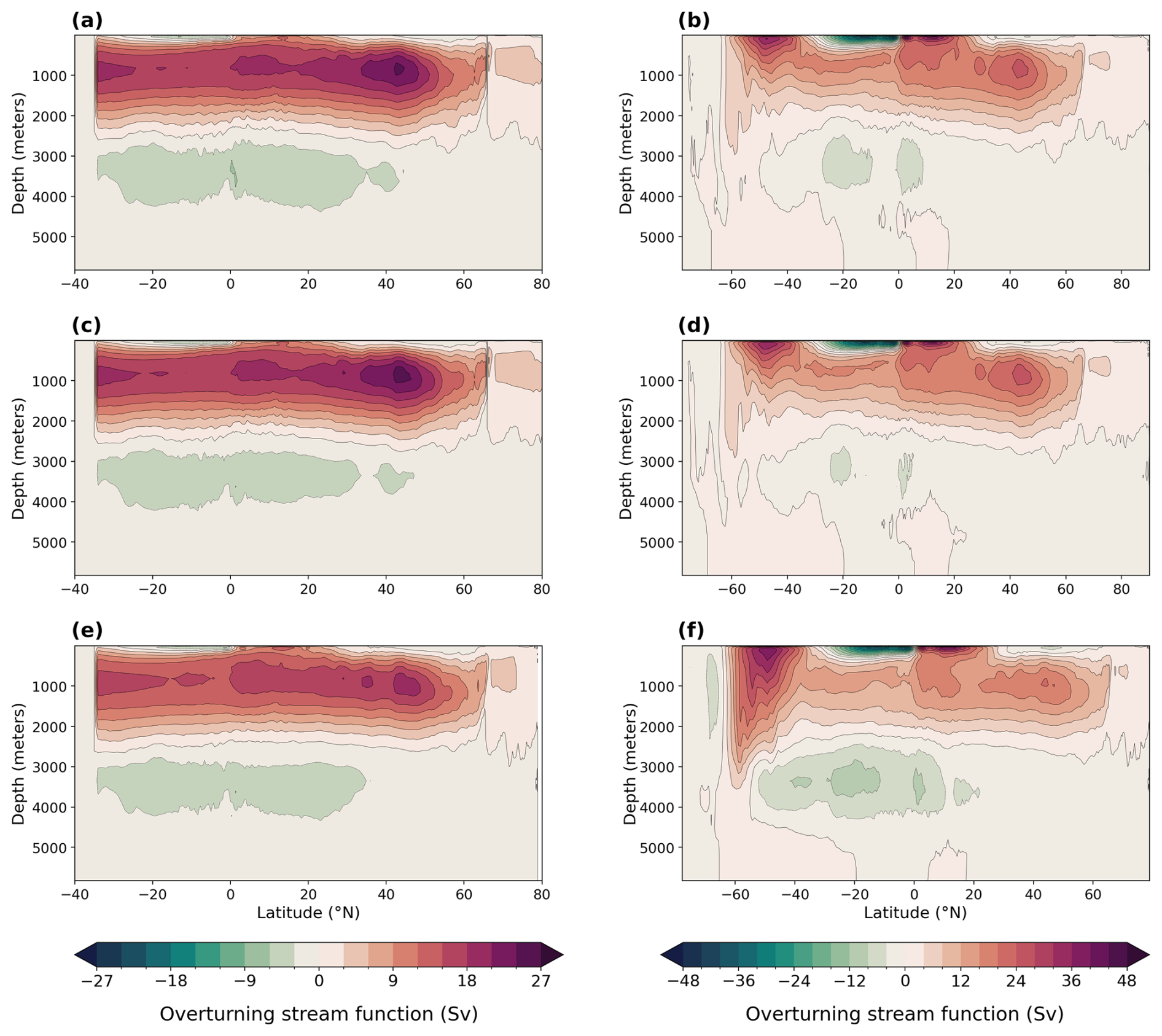
Figure 5 Meridional overturning streamfunction in sverdrups (Sv) for the Atlantic Ocean (a, c, e) and global (b, d, f). (a, b) LIG, (c, d) MIS 9e, and (e, f) PI.

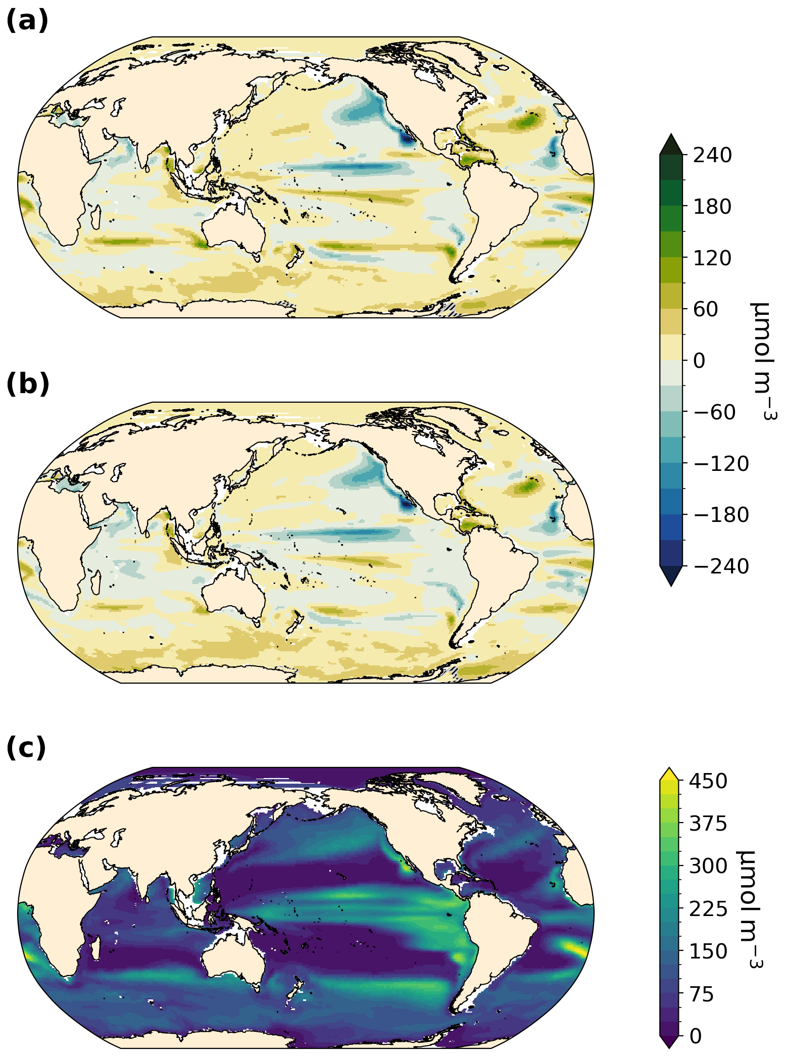
Figure 6 Detrital organic carbon concentration and anomalies in µmol C m⁻³ at 250 m depth. Statistically insignificant differences (p value > 0.01) are hatched and shaded in gray. Regions that are shallower than 250 m are shown in white. (a) LIG–PI, (b) MIS 9e–PI, and (c) PI.

3.1.2 North Atlantic Deep Water – colder and better ventilated

Figure 4a and d show that North Atlantic Deep Water (NADW) is more oxygenated in both MIS 9e and LIG compared to PI, with MIS 9e being more oxygenated than LIG at mid-depth between 40° S and 20° N. This is due to enhanced deepwater formation (Choudhury et al., 2022; Fig. 5) and stronger advection of NADW at depth leading to a decrease in AOU (Fig. 4c and f) and to lower temperatures of NADW in LIG and MIS 9e compared to PI (Figs. A2 and 4, middle column). The maximum value of the streamfunction in the Atlantic at 45° N reaches 23.6 Sv in our LIG simulation and 24.3 Sv in the MIS 9e simulation, compared to 19.9 Sv in the PI simulation. These simulated changes in NADW transport are associated with an advective–convective feedback mechanism involving the Subpolar Gyre (SPG), first described by Levermann and Born (2007). The SPG is stronger in our MIS 9e and LIG simulations than in PI (Fig. A4, left column), with an establishment of a third region of deep convection in the Labrador Sea in addition to the deep convection sites in the Norwegian Sea and south of the Greenland–Scotland Ridge (Fig. A3). During boreal winter (December to February), a stronger SPG results in stronger outcropping of isopycnals and in higher sea surface salinities (Fig. A4, right column) due to enhanced transport of subtropical saline waters. Both are preconditioning the surface waters for convection. The resulting horizontal surface density gradients maintain the strong gyre. The new convection site in the Labrador Sea contributes colder waters to the resulting North Atlantic Deep Water mass, leading to an overall colder NADW compared to PI (Fig. A2). Export production is enhanced over most of the North Atlantic Ocean in LIG and MIS 9e compared to PI and is therefore not one of the drivers of the increase in dissolved oxygen (Fig. 6).

3.1.3 North Pacific Intermediate Water – warmer and better ventilated

The North Pacific ocean above ∼ 2000 m is significantly more oxygenated in our LIG and MIS 9e simulations than in our PI simulation (Fig. 4g and j), with LIG being even more oxygenated than MIS 9e. The potential temperatures of the affected water masses are higher in both simulations compared to PI (Figs. A2 and 4h and k). The oxygenation is therefore solely due to changes in AOU, which shows strong negative anomalies (Fig. 4i and l). We can see a slight increase in ventilation during winter months in both simulations due to higher subduction rates in the western Bering Sea – along the coast of the Kamchatka Peninsula (Fig. A5). This leads to younger and better ventilated waters at 250 m depth circulating across the Pacific and then southward following the California Current (shown in Fig. A6). There is also a significant decrease in export production off the west coast of North America in LIG and MIS 9e compared to PI (Fig. 6). This is due to a weakening of the north-westerly winds causing a weakening of the coastal upwelling zones (Fig. A7, left column) contributing to the gain in oxygen at deeper layers (Fig. 3a and b). Furthermore, better ventilated subsurface waters can lead to a decrease in nutrient concentrations and therefore an overall reduction in nutrients transported to the surface via upwelling (Donald et al., 2024).

3.1.4 Oxygen minimum zones (OMZs) – no significant change

Figure 7 (left column) shows dissolved O₂ concentrations in hypoxic zones at 300 m depth. In our PI simulation, the model represents the large-scale patterns reasonably well in the tropical and subtropical Pacific but overestimates oxygen depletion within these zones (Fig. 7e and g). The simulated OMZ in the Atlantic ocean off the African coast is also overestimated in extent and intensity. Contrarily, oxygen depletion in the North Pacific and the Arabian Sea is underestimated at 300 m depth, but the North Pacific ocean becomes hypoxic at deeper levels (Fig. 7, right column).

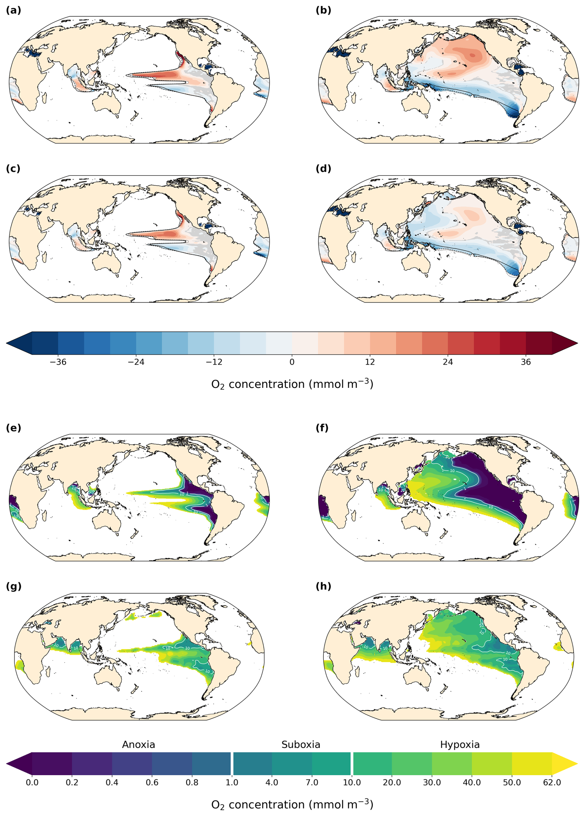
Figure 7 O₂ concentration and anomalies at 300 m depth in hypoxic zones (left) and vertical minimum of O₂ concentration and anomalies in hypoxic zones (right) in (a, b) LIG–PI, (c, d) MIS 9e–PI, (e, f) PI, and (g, h) World Ocean Atlas (WOA, 1965–2022). Black contour lines in panels (a)–(d) indicate the 62 mmol m⁻³ isolines for PI (solid), LIG (dotted), and MIS 9e (dashed). Statistically insignificant differences (p value > 0.01) are shaded in gray. Hypoxic zones are defined as zones where O₂ concentration at 300 m is below 62 mmol m⁻³ for panels (a), (c), (e), and (g) and where the vertical minimum of O₂ concentration is below 62 mmol m⁻³ for panels (b), (d), (f), and (h).

The extent and intensity of OMZs is very similar between the three simulations at 300 m depth (Fig. 7a and c). The Eastern Boundary Upwelling System off the coast of North America is weakened in our LIG and MIS 9e simulations compared to PI (Fig. A7), which leads to a decrease in nutrient availability at the surface (not shown), causing lower primary productivity and export production (Fig. 6). Consequently, AOU is significantly reduced in our LIG and MIS 9e simulations off the coast of California and Baja California (Fig. A8b and d), leading to an increase in oxygen in the northern hemispheric tropical Pacific OMZ that is partially compensated by a decrease in solubility due to higher water temperatures (Fig. A8a and c). The Eastern Boundary Upwelling System off Africa is also weakened (Fig. A7, right column) but does not affect the OMZ, which is situated further south. The OMZs in the southern hemispheric tropical Pacific and South Atlantic are slightly intensified in our LIG and MIS 9e simulations compared to PI, which is due to warmer waters and partially compensated by a decrease in AOU in these regions (Fig. A8).

The right column of Fig. 7 shows the minimum of dissolved oxygen in the water column. The model represents the extent of hypoxic waters well in the Pacific Ocean but underestimates the extent in the Indian Ocean and, again, misses the OMZ in the Arabian Sea. The extent of the South Atlantic OMZ is overestimated. The intensity of oxygen loss is overestimated in the eastern regions of all OMZs (Fig. 7f and h). Differences between the simulations show that the mid- to high-latitude North Pacific is significantly more oxygenated in LIG and, to a lesser extent, in MIS 9e, as discussed in Sect. 3.1.3. The southern and western parts of the Pacific hypoxic zones as well as most of the hypoxic zones in the Atlantic Ocean become more oxygen depleted in LIG and MIS 9e compared to PI. The minimum oxygen concentration in the water column shifts to deeper depths in the northern hemispheric Pacific and to shallower depth in most of the southern hemispheric Pacific (Fig. A9).

Table 2 Total volume (percentage) of oxygen-depleted water masses.

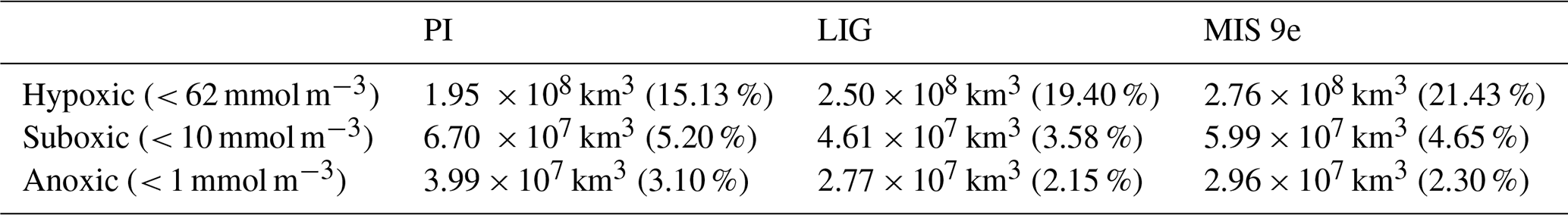
The global ocean is overall less oxygenated in MIS 9e and LIG compared to PI, and this is also reflected in the total volume of hypoxic waters (< 62 mmol m⁻³), which is 5 % larger in these simulations (Table 2). However, the suboxic (< 10 mmol m⁻³) and anoxic (< 1 mmol m⁻³) zones are smaller in our LIG and MIS 9e simulations, mainly due to the oxygenation of the North Pacific Ocean (Sect. 3.1.3).

3.2 Oxygenation of the Mediterranean Sea – large-scale hypoxia

The Mediterranean Sea is a semi-enclosed sea which is linked to the Atlantic Ocean via the relatively narrow and shallow (< 900 m) Strait of Gibraltar. Changes in large-scale circulation therefore impact the Mediterranean Sea only moderately, although the opposite is not true, as the Mediterranean outflow impacts the circulation in the Atlantic Ocean (Barbosa Aguiar et al., 2015). There have been numerous time intervals during past interglacials when some regions of the Mediterranean Sea became anoxic, prompting us to analyze changes in simulated dissolved O₂ in the Mediterranean Sea in this section.

Table 3 Volume (percentage) of oxygen-depleted water masses in the Mediterranean Sea.

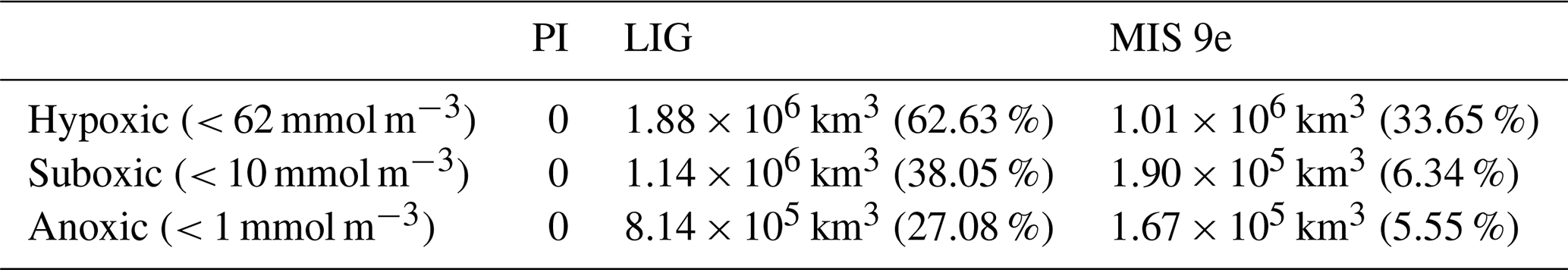
The mean O₂ concentration in the Mediterranean Sea equals 218.7 mmol m⁻³ in our PI simulation compared to 106.2 and 61.6 mmol m⁻³ in our MIS 9e and LIG simulations, respectively. In the LIG simulation 63 % of Mediterranean waters are hypoxic, with dissolved oxygen concentrations below 62 mmol m⁻³, and 27 % are anoxic (less than 1 mmol m⁻³). The MIS 9e simulation is not quite as depleted in oxygen in the Mediterranean Sea, with 34 % of the total volume being hypoxic and 5.6 % anoxic (Table 3).

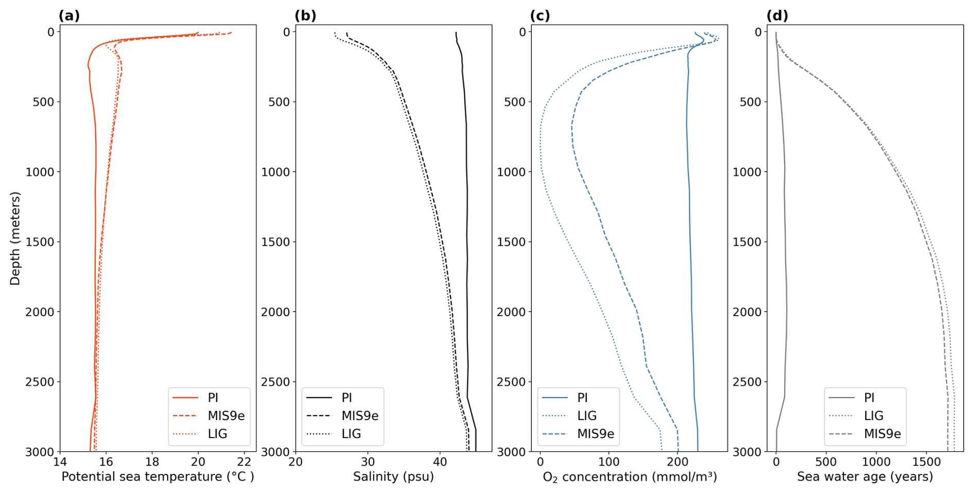
Figure 8 Zonal and meridional mean vertical profiles in the Mediterranean Sea for PI (solid lines), LIG (dotted lines), and MIS 9e (dashed lines). (a) Potential temperature in degrees Celsius (°C), (b) salinity in practical salinity units (psu), (c) O₂ concentration in mmol m⁻³, and (d) seawater age since last surface contact in years. Note that the maximum possible water age equals the length of the simulation and might therefore underestimate the water age for very old water masses.

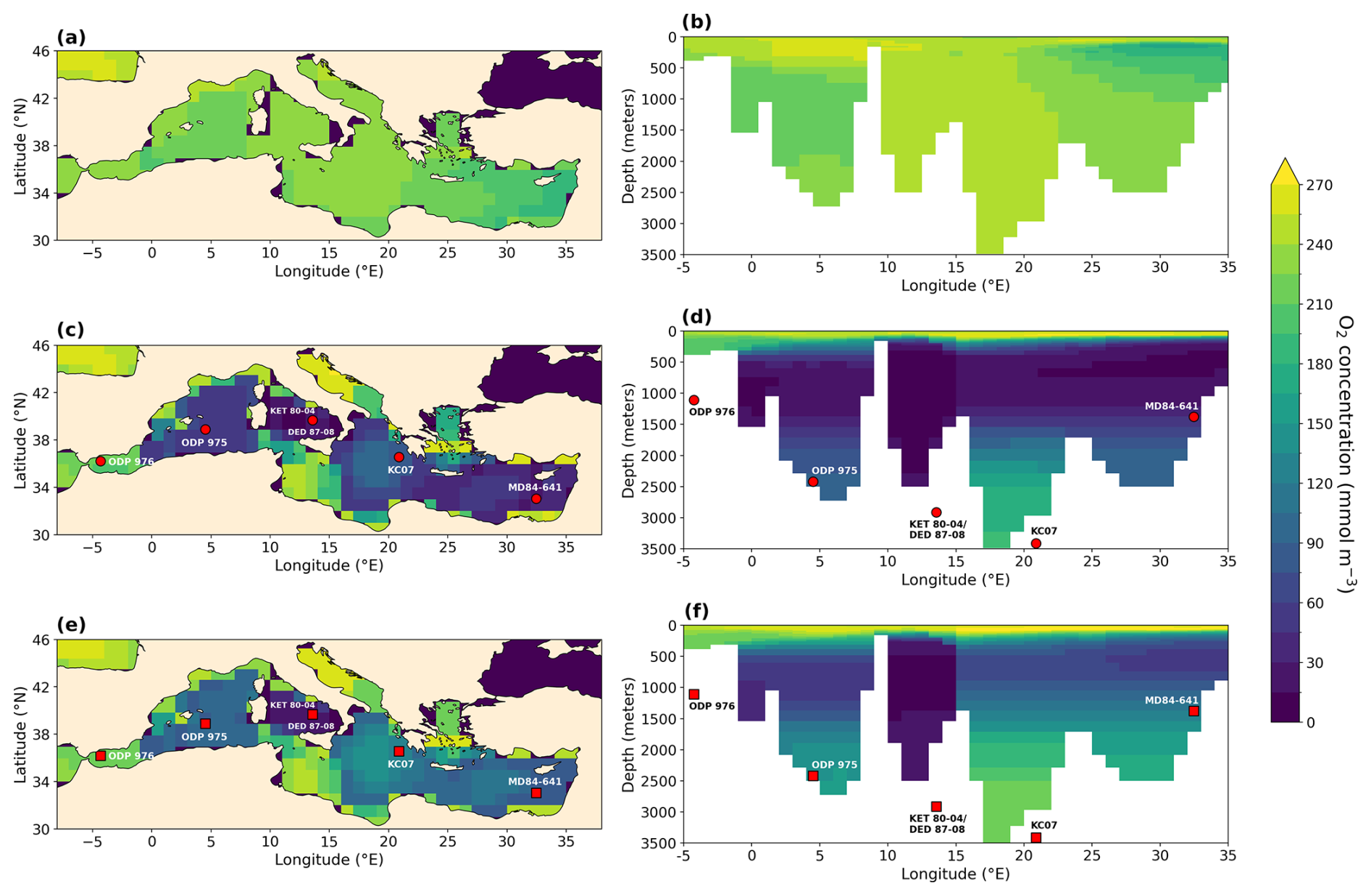
Figure 9 Vertical mean O₂ concentration (a, c, e) and meridional mean O₂ concentration (b, d, f) in the Mediterranean Sea in mmol m⁻³ for PI (a, b), LIG (c, d), and MIS 9e (e, f). Symbols represent core sites discussed in the text.

The depletion of dissolved oxygen in the MIS 9e and LIG simulations is greatest in intermediate water masses (Figs. 8c and 9, right column), with horizontally averaged O₂ concentrations dropping to 50 mmol m⁻³ in MIS 9e and reaching anoxic values in LIG between 500 and 1000 m depth (Fig. 8c). This deoxygenation is caused by a strong pycnocline due to a significant freshening and warming of the surface layers (Fig. 8a and b) that prevents mixing between surface and deeper layers and increases the water ages of intermediate and deep water masses (Fig. 8d). While there is deep water formation in winter months in the Ionian Sea with seasonal mean winter ventilation depth reaching 489 m, and to a lesser extent in the southern Adriatic Sea and east of the Gulf of Lion (west of Corsica) in our PI simulation, winter-mean mixed layer depths do not exceed 97 and 106 m in our LIG and MIS 9e simulations, respectively (Fig. A10).

Figure 9 shows that the central Mediterranean Sea is severely oxygen depleted in both LIG and MIS 9e simulations, with O₂ concentrations dropping to zero in the Tyrrhenian Sea below 100 m depth. This is in qualitative agreement with the appearance of organic-rich dark layers in core DED 87-08 (39°42^′ N, 13°35^′ E; 2965 m; Fontugne and Calvert, 1992; Kallel et al., 2000) during eastern Mediterranean Sapropel events S5 (121.5–128.3 ka; Grant et al., 2016) and S10 (∼ 332 ka; Konijnendijk et al., 2014). Core KET 80-04 (39°40^′ N, 13°34^′ E; 2909 m) also shows evidence of anoxic conditions during S5 in the Tyrrhenian Sea (Kallel et al., 2000).

The eastern Mediterranean basin is also oxygen depleted, especially in our LIG simulation. The simulated oxygen depletion in the Levantine Sea is in agreement with core MD 84-641 (33°02^′ N, 32°38^′ E; 1375 m), which recorded a strong sapropel event (S5) at the LIG (4.52 % total organic carbon (TOC)) and a less strong sapropel event (S10) at MIS 9e (2.5 % TOC) (Fontugne and Calvert, 1992; Melki et al., 2010). Our results are also in agreement with Andersen et al. (2018), who find water mass ages of 1030 (+820/−520 years) in the deep eastern Mediterranean Sea (compared to ∼ 100 years today) at the end of S5, and with Sweere et al. (2021), who find euxinic conditions during S5 in the Levantine Sea.

The Ionian Sea is better oxygenated than the Levantine Sea in our simulations, but conditions at intermediate depths are still hypoxic in the MIS 9e simulation, dropping to 52.4 mmol m⁻³ and reaching anoxic values in the LIG simulation. Core KC07 (20°53^′ N, 36°34^′ E; 3410 m) records rich organic layers during both S5 and S10 (Köng et al., 2017) but is situated at a depth where our simulations show higher oxygen concentrations. It should be noted that oxygen concentrations in the deep waters in the Ionian Sea are still drifting in our simulations and might reach suboxic values if integrated for longer.

In the western Mediterranean, sapropels are less distinctive than in the eastern Mediterranean, but they can still be detected in terms of higher-than-background organic carbon content. ODP leg 161 drilled five sites throughout the western Mediterranean and found that sapropel TOC values decrease to the west and are lowest in the Alboran Sea (Murat, 1999). Cores 975 (38°53.795^′ N, 04°30.595^′ E; 2416 m), 976 (36°12.32^′ N, 04°18.760^′ W; 1108 m), 977 (36°01.907^′ N, 01°957.319^′ W; 1984 m), and 979 (35°43.427^′ N, 03°12.353^′ W; 1062 m) all record higher organic carbon layers between 122 and 128 ka and between 328 and 331 ka, and the S5 event is color-banded in site 975, while the S10 event is homogeneous (Murat, 1999). This east–west gradient is reflected in our simulations, where waters near the Strait of Gibraltar are better oxygenated than waters in the Alboran Sea.

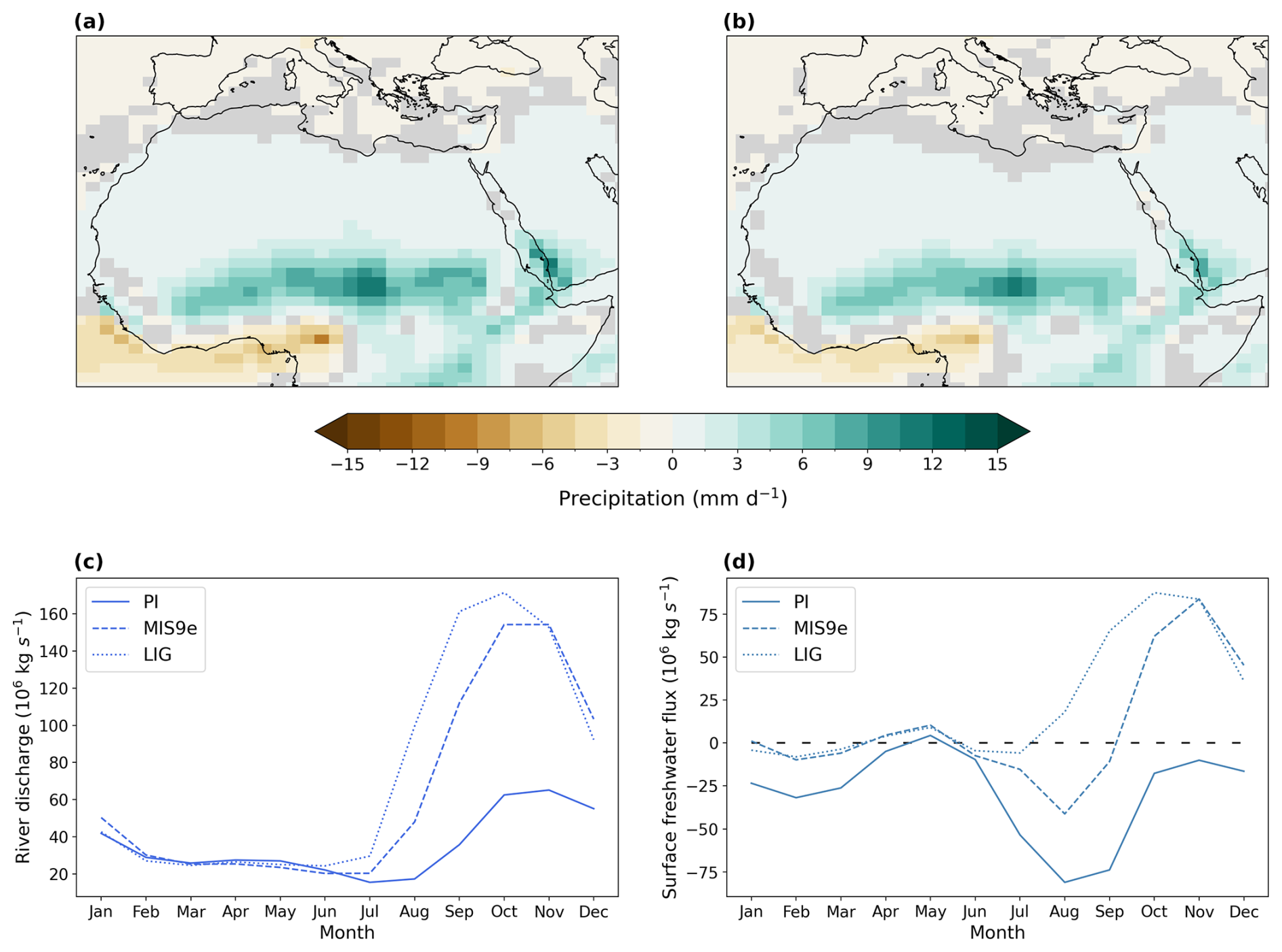
Figure 10 Anomalies of precipitation in North Africa during boreal summer (JJA) in mm d⁻¹ for (a) LIG–PI and (b) MIS 9e–PI; (c) seasonal freshwater discharge from all rivers into the Mediterranean Sea for PI (solid line), LIG (dotted line), and MIS 9e (dashed line) in 10⁶ kg s⁻¹ and (d) seasonal freshwater surface fluxes (precipitation + runoff − evaporation) into the Mediterranean Sea in 10⁶ kg s⁻¹ for PI (solid line), LIG (dotted line), and MIS 9e (dashed line). Statistically insignificant differences (p value > 0.01) are shaded in gray in panels (a) and (b). Monthly values are processed following paleo-seasonal adjustments (Bartlein and Shafer, 2019) with reference dates of 127 and 333 ka for LIG and MIS 9e, respectively. The x axis in panels (c) and (d) represents months according to the present-day calendar.

The North African monsoon expands significantly into the Sahara region in our LIG (Yeung et al., 2021) and MIS 9e simulations, hence causing an intensification of precipitation during the wet season in North Africa (Yeung et al., 2021; Menviel et al., 2021). Rainfall in the Sahara region increases locally by up to +12.0 mm d⁻¹ in LIG and +10.9 mm d⁻¹ in MIS 9e during boreal summer (JJA) compared to PI (Fig. 10a and b). This excess rainfall causes excess freshwater runoff that enters the Mediterranean basin mainly through the Nile Delta. Although North African monsoon intensity peaks between June and August, outflow into the Mediterranean Sea reaches its maximum in autumn between September and November (Fig. 10c and d). This time lag of about 3 months is caused by the river routing timescale embedded in the ACCESS-ESM1.5 model (Total Runoff Integrating Pathways (TRIP) river routing; Oki et al., 1999) and is similar to the observed timescale of river routing.

The annual-mean surface freshwater flux into the Mediterranean Sea (precipitation + river runoff − evaporation) is equal to −344 × 10⁶ kg s⁻¹ in our PI simulation compared to +248 × 10⁶ and +130 × 10⁶ kg s⁻¹ in our LIG and MIS 9e simulations, respectively. These positive fluxes cause freshening of the surface layers, stratification, and eventually deoxygenation of the Mediterranean Sea in our simulations (Fig. 1b). Compared to MIS 9e, the North African monsoon intensification is more pronounced in the LIG simulation (Fig. 10a and b), leading to higher river runoff (Fig. 10c). Sea surface salinities decrease at a faster rate and lead to stratification and deoxygenation earlier than in the MIS 9e simulation (Fig. 1b). The difference in oxygenation between LIG and MIS 9e is thus mainly due to the difference in the length of time during which the Mediterranean Sea is stratified, although small changes in biological productivity and export production (not shown) also contribute. It should be noted that oxygen levels in the Mediterranean Sea are still drifting in both simulations and that the equilibrium values are lower than what is presented here.

4 Discussion

The oxygenation of the world's oceans is very similar in our LIG and MIS 9e simulations and quite different compared to our PI simulation. These differences are primarily due to circulation changes and changes in export production and secondarily due to the solubility effect. The large-scale ocean circulation patterns, including AABW, NADW, and the ventilation of the North Pacific Ocean, are therefore very sensitive to the latitudinal and seasonal distribution of incoming solar radiation in the ACCESS ESM1.5 and less sensitive to changes in greenhouse gas concentrations within the range of these three interglacials. The insolation anomalies are indeed quite similar for LIG and MIS 9e (Fig. A1), while the greenhouse gas forcing is highest for MIS 9e and lowest for LIG, with PI being in the middle (Table 1).

While quantitative records of past oxygenation are difficult to reconstruct with proxies (Hoogakker et al., 2025), qualitative records exist. For the more recent Pleistocene period, most records looking at past ocean oxygenation have focused on glacial–interglacial variations; for summaries see Jaccard and Galbraith (2012) and Moffitt et al. (2015). Stott et al. (2000) used epibenthic foraminifera carbon isotopes to make inferences of intermediate water ventilation and oxygenation in the northeast Pacific and suggested that waters above 2000 m depth were less oxygenated during MIS 5e. If the proposed relationship between benthic foraminifera carbon isotopes and apparent oxygen utilization holds, then overall reduced carbon isotopes during MIS 5e (Bengtson et al., 2021) would imply an overall decrease in global ocean oxygenation, agreeing with our simulations. There is also evidence for reduced AABW formation and a decrease in dissolved oxygen in the Southern Ocean based on redox elements (Hayes et al., 2014; Glasscock et al., 2020).

Oxygen minimum zones (OMZs) have expanded and contracted repeatedly in the past in response to global changes in climate (Jaccard and Galbraith, 2012). To the authors' knowledge, there is no global modeling study analyzing the extent and magnitude of OMZs during MIS 5e and MIS 9e. Simulating OMZs with earth system models is very challenging, because low oxygen concentrations are the result of a subtle balance between two large opposing processes: the physical transport of oxygen-rich waters into the region of interest and the local flux of particulate matter and remineralization. Climate models are not very skilled in representing these dynamics, mostly because their resolution does not resolve equatorial dynamics well enough. Another problem is the simple representation of biology and geochemistry in the majority of current state-of-the-art models. The ACCESS ESM1.5 is not an exception. While the extent of the OMZs in the tropical Pacific is reasonably well represented, there are deficits in other regions. Our results show that relatively small changes in circulation, such as the subtle increase in ventilation of the upper North Pacific Ocean in our LIG and MIS 9e simulations, can have a significant impact on oxygen concentrations, emphasizing the need of a realistic representation of physical circulation when simulating oxygen. For example, cores LV-28-44-3 (52°02.514^′ N, 153°05.949^′ E; 684 m) in the eastern Sea of Okhotsk (Matul et al., 2016) and MR0604-PC07A (51°16^′56^′′​​​​​​​ N, 149°12^′60^′′​​​​​​​ E; 1247 m) in the central Sea of Okhotsk (Jimenez-Espejo et al., 2018) recorded intervals of suboxic conditions during MIS 5e. While our simulation points to suboxic waters east of the Kamchatka Peninsula, the waters west of the peninsula are well oxygenated (Fig. 7). It should be noted that these cores were retrieved from a semi-isolated marginal basin and are influenced by small-scale local circulation patterns that are not well resolved in the ACCESS ESM1.5.

We find that the main Eastern Boundary Upwelling Systems in the North Pacific and Atlantic Oceans are weaker in the LIG and MIS 9e simulations compared to PI. This is consistent with high sea surface temperatures and faunal composition off the Canary Islands during MIS 5e (Muhs et al., 2014; Maréchal et al., 2020) and microfossil assemblages from MIS 5e off the coast of northern California (Poore et al., 2000). However, Si $/$ Ti, Cd $/$ Al, and Ni $/$ Al records from core MD02-2508 (23°27.91^′ N, 111°35.74^′ W; 606 m) suggest that biological productivity was high during MIS 5e further south, off the coast of Baja California (Cartapanis et al., 2014), which is contrary to our results, although some upwelling is still present in our LIG and MIS 9e simulations. Coastal upwelling may have been similar or enhanced during MIS 5e and MIS 9e along the southeast African margin (Pichevin et al., 2005; Ufkes and Kroon, 2012), expanded along the Brazil margin during MIS 5e (Lessa et al., 2017), and increased at higher latitudes during MIS 5e and MIS 9e (Yao et al., 2024). This agrees broadly with the simulated patterns of detrital organic carbon concentration anomalies.

The Mediterranean's sedimentary record is punctuated by periodic deep-sea anoxic events (Sachs and Repeta, 1999; Rohling et al., 2015; Rush et al., 2019) that manifest themselves in layers with elevated organic carbon concentrations (sapropels) and are strongly associated with times of African monsoon intensification. We find monsoon intensification in our LIG and MIS 9e simulations, enhanced river runoff, and a freshening of the surface layers of the Mediterranean Sea. The resulting vertical stratification leads to anoxic conditions in the east Mediterranean Sea in our LIG simulation and hypoxic conditions in our MIS 9e simulation. The Tyrrhenian Sea is anoxic in both simulations, and the west Mediterranean shows an east–west gradient of oxygenation that is qualitatively in agreement with sediment data. It should be noted, however, that the ACCESS ESM1.5 is a global model with relatively coarse horizontal resolution (1° × 1° in the Mediterranean Sea). Such coarse-resolution model cannot be expected to simulate Mediterranean circulation skillfully. There are three main sites of deep water formation in the Mediterranean Sea in today's climate. Western Mediterranean deep water is formed during winter in the Gulf of Lion. Eastern Mediterranean deep water formation occurs in two sites, the Adriatic Sea, where bottom water is formed in winter and exits through the Strait of Otranto, and the Rhodes Gyre in the Levantine Basin. In our PI simulation, the main deep water formation occurs in the Ionian Sea, and to a lesser extent in the southern Adriatic Sea and east of the Gulf of Lion. Our results should therefore be taken as a qualitative indication of enhanced stratification and oxygen loss without putting too much trust into simulated regional changes. For example, Tesi et al. (2024) find shallow water euxinia during S5 on the Adriatic Shelf due to a shutdown of North Adriatic Dense Water formation. This region remains well ventilated in our simulations. In addition, note that Mediterranean oxygen content is still drifting in our LIG and MIS 9e runs. As a result, MIS 9e could reach an oxygen loss similar to LIG on a longer timescale (Fig. 1).

Our study shows that even relatively small changes in boundary conditions can lead to large changes in ocean circulation, upwelling systems, export production, and ocean oxygenation. While our results cannot directly inform on future changes in ocean oxygenation, there might be some similarities. Ocean temperatures and ocean stratification are projected to continue to increase until atmospheric CO₂ concentrations finally plateau. Current ocean deoxygenation is therefore not easily reversible and will persist for centuries (Oschlies, 2021). There will be physiological and morphological impacts on organisms, including reduced growth for a vast range of taxonomic groups (Sampaio et al., 2021). Exposure to low-oxygen conditions has also been associated with a delay in when fish produce eggs, a reduction of the number of eggs fish produce, and blindness (Landry et al., 2007; McCormick and Levin, 2017). The metabolic demand of oxygen increases with water temperature, and when combined with deoxygenation, this can lead to respiratory distress, followed by respiratory failure and death (Clarke et al., 2021). Over 50 mass mortality events due to hypoxia have been recorded in the tropics to date (Altieri et al., 2017). The consequences of deoxygenation for fisheries and the world's future food supply could thus be serious (Oschlies et al., 2018; Rose et al., 2019).

Here we perform a snapshot experiment of the peak LIG and MIS 9e climates with a single model. These simulations thus only represent an equilibrium response to peak interglacial conditions and do not represent potential transient climatic changes associated with the end of deglaciations or abrupt climate changes linked to continental ice-sheet melting. In addition, the dissolved O₂ content simulated in these experiments is very dependent on the simulated oceanic circulation. The state of the ocean circulation during these interglacials is, however, unclear. Transient simulations through whole interglacial and multi-model intercomparisons would be preferable and give a better indication of the robustness and uncertainties of past oxygenation patterns and their variability (Cartapanis et al., 2014). We hope that other modeling groups will consider analyzing ocean oxygenation during past interglacials. Oxygen concentration is a variable with extremely long equilibration times, so caution should be taken when climate models are not integrated for at least 1000 years, preferably longer, and the drift in the deep ocean is still significant.

5 Conclusions

We integrated three equilibrium simulations with Australia's earth system model ACCESS ESM1.5 under preindustrial (PI), Last Interglacial (LIG, 127 ka), and MIS 9e (333 ka) boundary conditions. The LIG and MIS 9e simulations show similar anomalies in large-scale oxygenation pointing to the fact that circulation patterns and oxygen concentrations are more sensitive to the distribution of incoming solar radiation than to greenhouse gas concentrations within the range of these three interglacials. Antarctic Bottom Water (AABW) is weaker and warmer, leading to deoxygenation mostly due to higher oxygen utilization and, to a lesser extent, the solubility effect. North Atlantic Deep Water (NADW) is overall cooler and better ventilated, leading to higher in situ oxygen concentrations. Water masses in the upper 2000 m of the North Pacific are both warmer and higher in oxygen content, due to enhanced subduction in the Bering Sea and a reduction in export production off the coast of North America. These anomalies are more pronounced in the MIS 9e simulation than in the LIG simulation, with the exception of the North Pacific Ocean, where the oxygenation anomaly is strongest in the LIG simulation. While the global ocean is overall less oxygenated in MIS 9e and LIG compared to PI, the volume of suboxic and anoxic waters is smaller in MIS 9e and LIG, mainly due to the oxygenation of the North Pacific Ocean. The Mediterranean Sea is the exception, where oxygen is significantly more depleted in MIS 9e and LIG compared to PI, due to an intensification and expansion of the African monsoon, enhanced runoff, and resulting freshening of surface waters and stratification. In the LIG simulation, 30 % of the total seawater volume in the Mediterranean Sea is anoxic (< 1 mm m⁻³) and 63 % is hypoxic (< 62 mm m⁻³). This deoxygenation is not quite as pronounced in the MIS 9e simulation with 6 % of anoxic waters and 34 % of hypoxic waters. Dissolved oxygen concentrations are still drifting in both simulations, even after integration times of well over 1500 years.

The simulation of ocean oxygen concentrations is challenging, as oxygen levels depend on complex physical and biogeochemical processes that must be represented correctly in a climate model to simulate oxygen realistically. State-of-the-art earth system climate models systematically underestimate the observed rates of oxygen loss and are also not very skillful in reproducing the observed patterns of deoxygenation (Oschlies et al., 2017, 2018). In this study, we confirmed that subtle changes in ocean circulation can have significant impact on oxygen concentrations. For trustworthy future projections, high-resolution ocean models are therefore needed to represent the relevant ocean circulation patterns as well as possible, but these models are computationally expensive. Oceanic oxygen takes centuries to adjust, and we currently lack computer power to run high-resolution models for the timescales needed for initialization and equilibrium responses. Another important challenge is the representation of biogeochemical processes in models, as our knowledge of coupled biogeochemical processes is still incomplete.

Appendix A

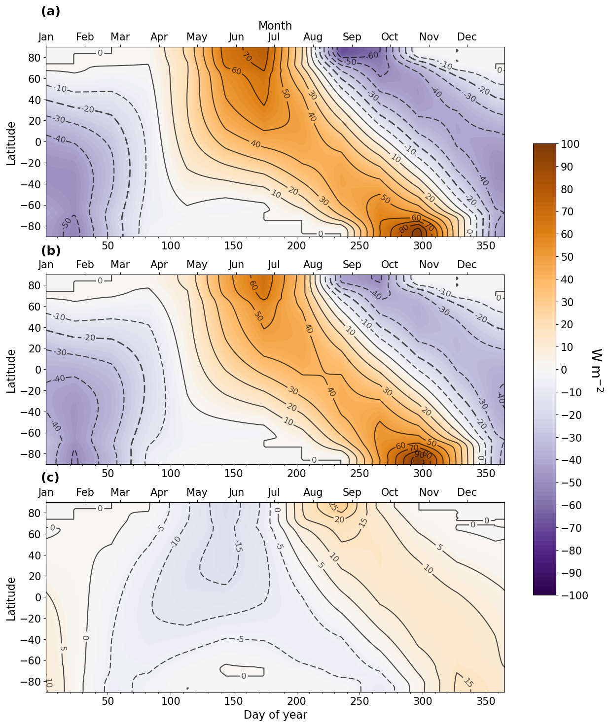
Figure A1 Insolation anomalies (W m⁻²) across latitudes and days of year. (a) LIG–PI, (b) MIS 9e–PI, and (c) MIS 9e–LIG. The bottom x axis represents the day of year, and the top x axis represents months according to the present-day calendar.

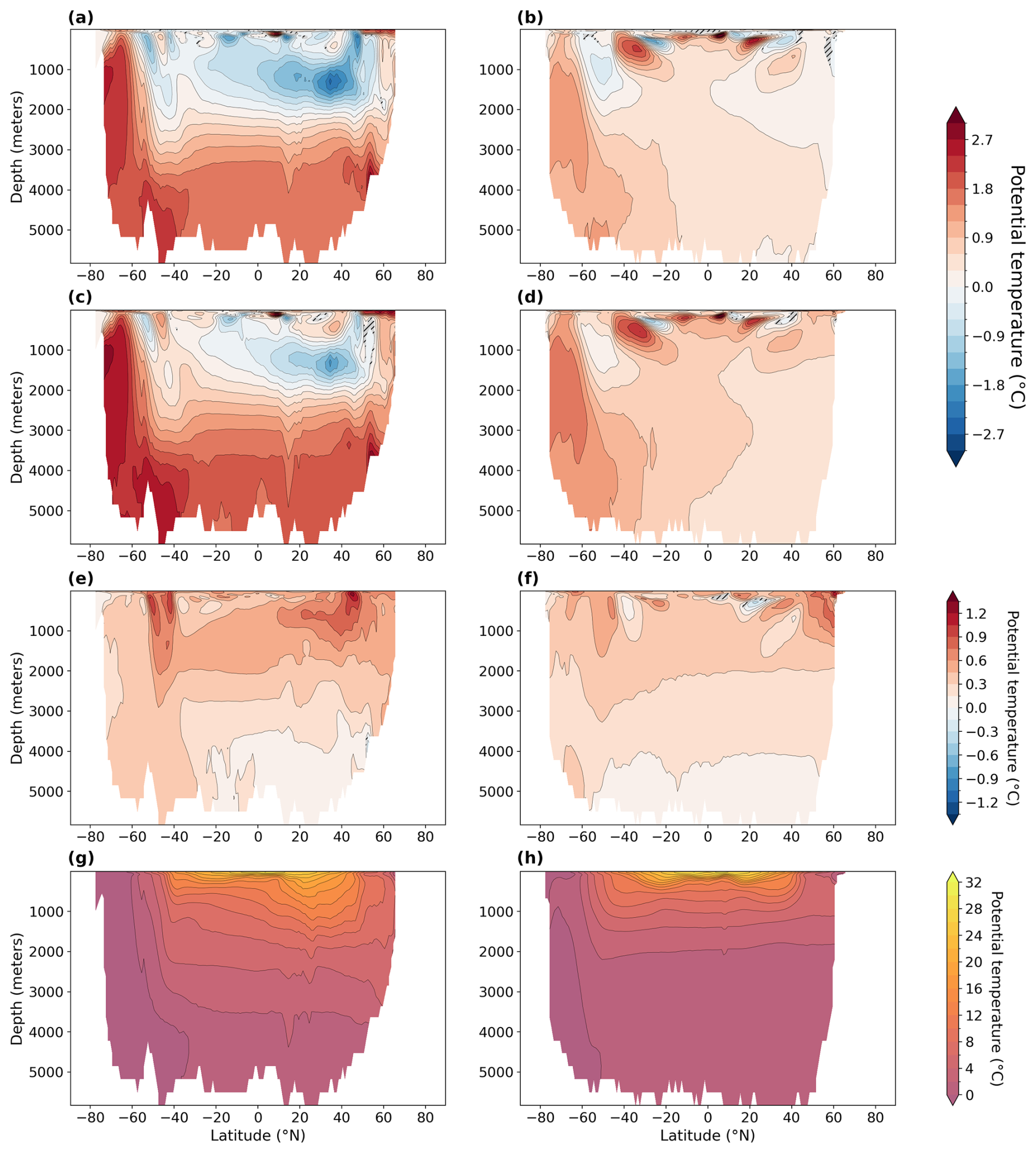
Figure A2 Zonally averaged potential temperature in degrees Celsius (°C) (g, h) and anomalies (a–f) in the Atlantic Ocean (left) and in the Pacific Ocean (right). Statistically insignificant differences (p value > 0.01) are hatched and shaded in gray. (a, b) LIG–PI, (c, d) MIS 9e–PI, (e, f) MIS 9e–LIG, and (g, h) PI.

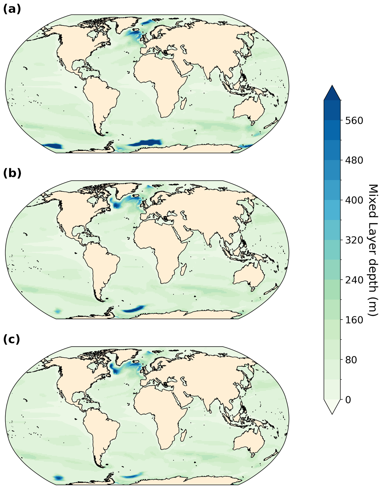
Figure A3 Annual-mean mixed layer depth in meters (m). (a) PI, (b) LIG, and (c) MIS 9e.

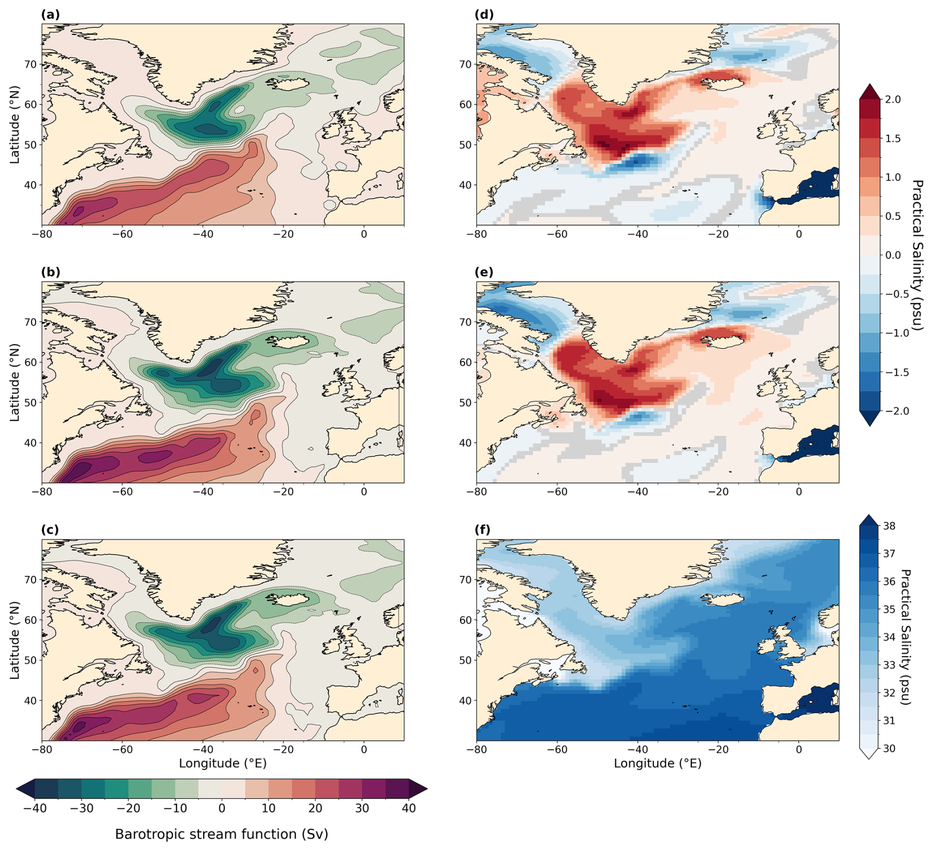
Figure A4 Depth-integrated barotropic stream function in the North Atlantic Ocean averaged during boreal winter in sverdrups (Sv) (DJF; a–c) and sea surface salinity in practical salinity units (psu) (f) and anomalies (d, e) in the North Atlantic Ocean averaged over boreal winter months (DJF). Statistically insignificant differences (p value > 0.01) are shaded in gray. Mean over DJF months is processed following paleo-seasonal adjustments (Bartlein and Shafer, 2019) with reference dates of 127 and 333 ka for LIG and MIS 9e, respectively. (a) PI, (b) LIG, (c) MIS 9e, (d) LIG–PI, (e) MIS 9e–PI, and (f) PI.

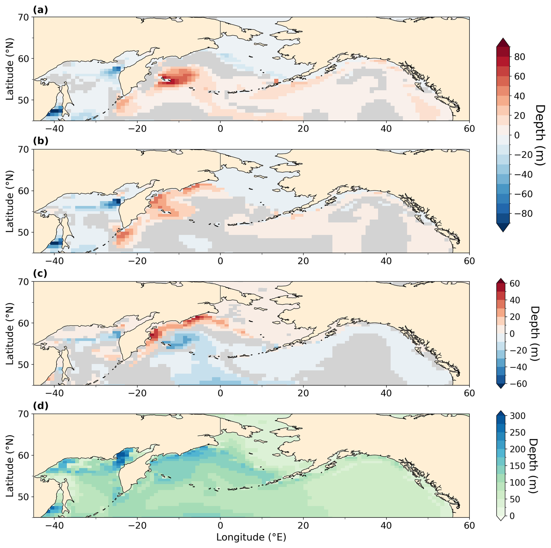
Figure A5 Mixed layer depth and anomalies in the North Pacific ocean averaged during boreal winter (DJF) in meters (m). Statistically insignificant differences (p value > 0.05) are shaded in gray. Mean over DJF months is processed following paleo-seasonal adjustments (Bartlein and Shafer, 2019) with reference dates of 127 and 333 ka for LIG and MIS 9e, respectively. (a) LIG–PI, (b) MIS 9e–PI, (c) MIS 9e–LIG, and (d) PI.

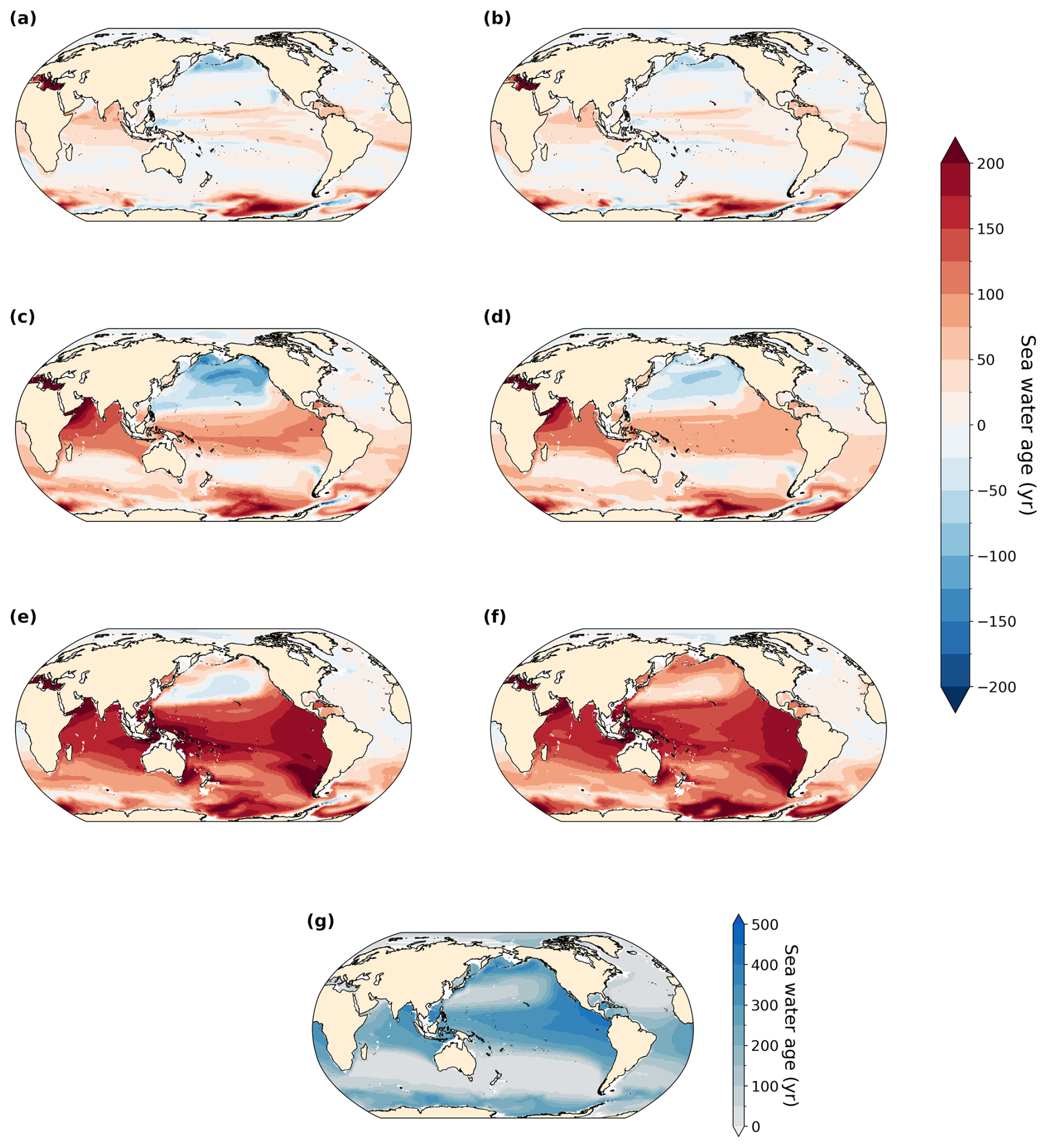
Figure A6 Water age since last surface contact in years (g) and anomalies (a–f) for LIG–PI (a, c, e) and MIS 9e–PI (b, d, f). (a, b) 250 m depth, (c, d) 500 m depth, (e, f) 1000 m depth, and (g) 500 m PI reference. Statistically insignificant differences (p value > 0.01) are shaded in gray.

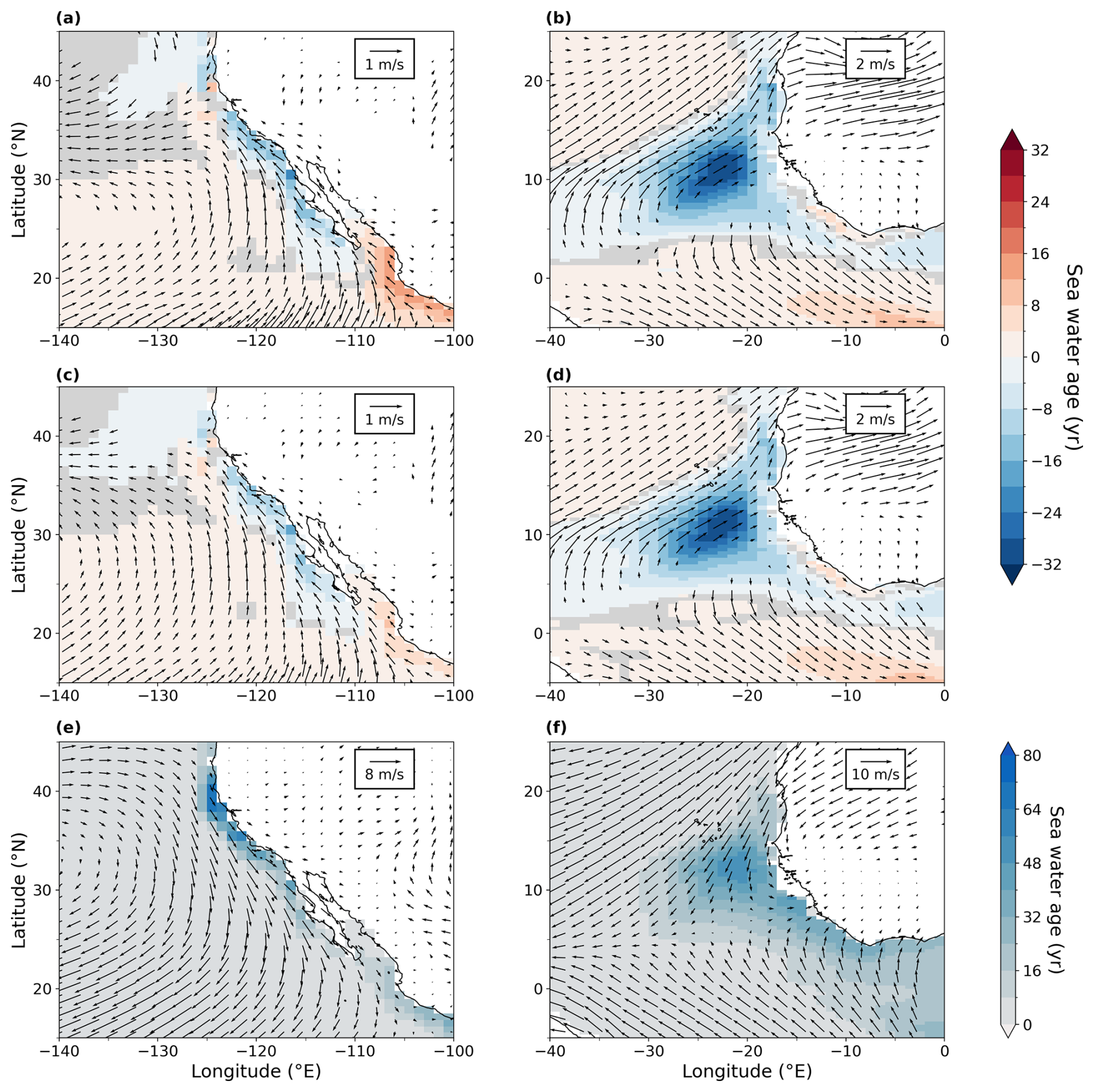
Figure A7 Annual-mean water age since last surface contact at 50 m depth overlaid with annual-mean surface wind at 10 m (e, f) and anomalies (a–d) off the west coast of North America (a, c, e) and off West Africa (b, d, f). (a, b) LIG–PI, (c, d) MIS 9e–PI, and (e, f) PI. Statistically insignificant differences of water age (p value > 0.01) are shaded in gray, and statistically insignificant wind difference vectors are not represented.

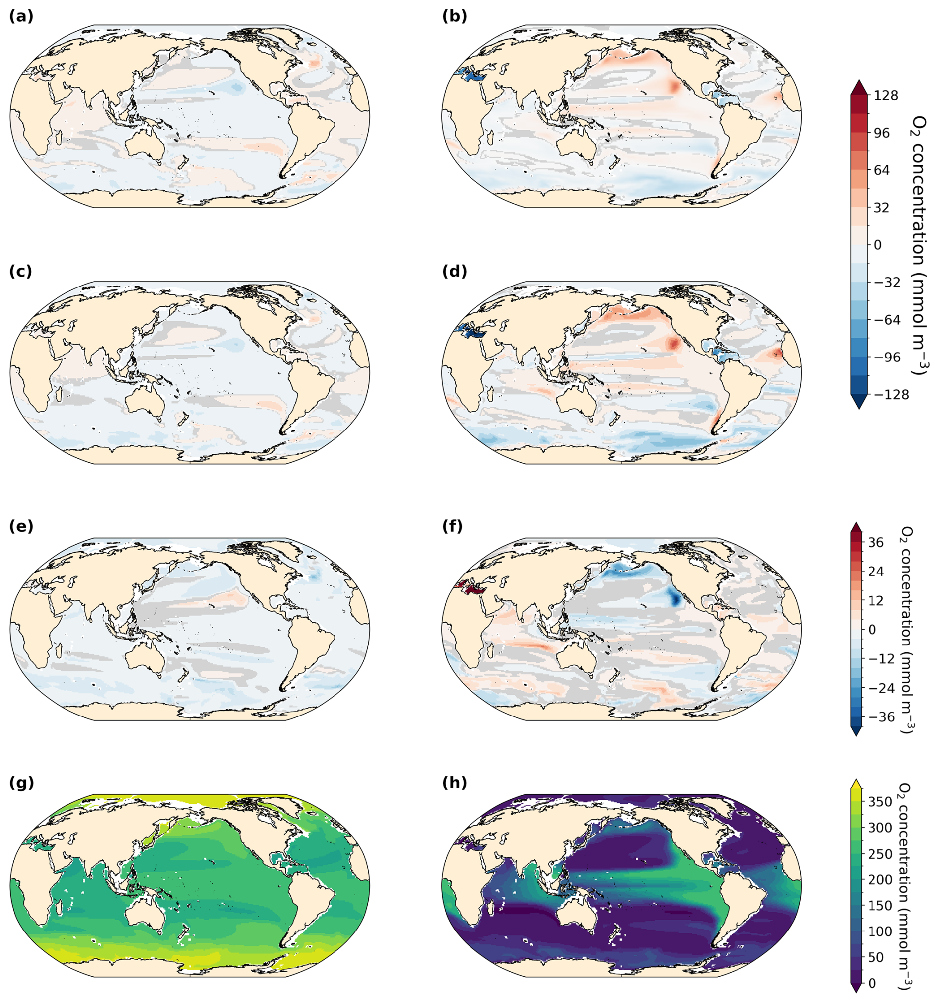
Figure A8 Saturated O₂ concentration (left) and $-\mathrm{1}\cdot$AOU (apparent oxygen utilization, right) at 300 m depth. Statistically insignificant differences (p value > 0.01) are shaded in gray. Anomalies of LIG–PI (a, b), MIS 9e–PI (c, d), and MIS 9e–LIG (e, f). Full fields for PI are shown in panels (g) and (h). To facilitate the comparison between oxygen solubility and oxygen utilization, we multiplied AOU by −1.

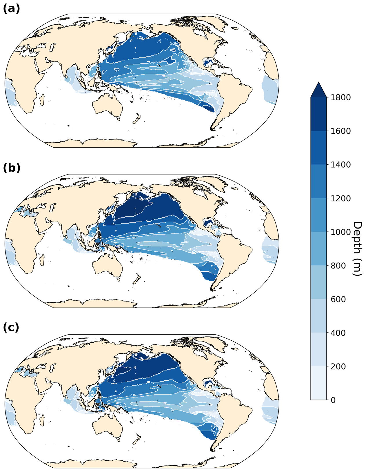
Figure A9 Depth of minimum O₂ concentration in hypoxic zones (< 62 mmol m⁻³). (a) PI, (b) LIG, and (c) MIS 9e.

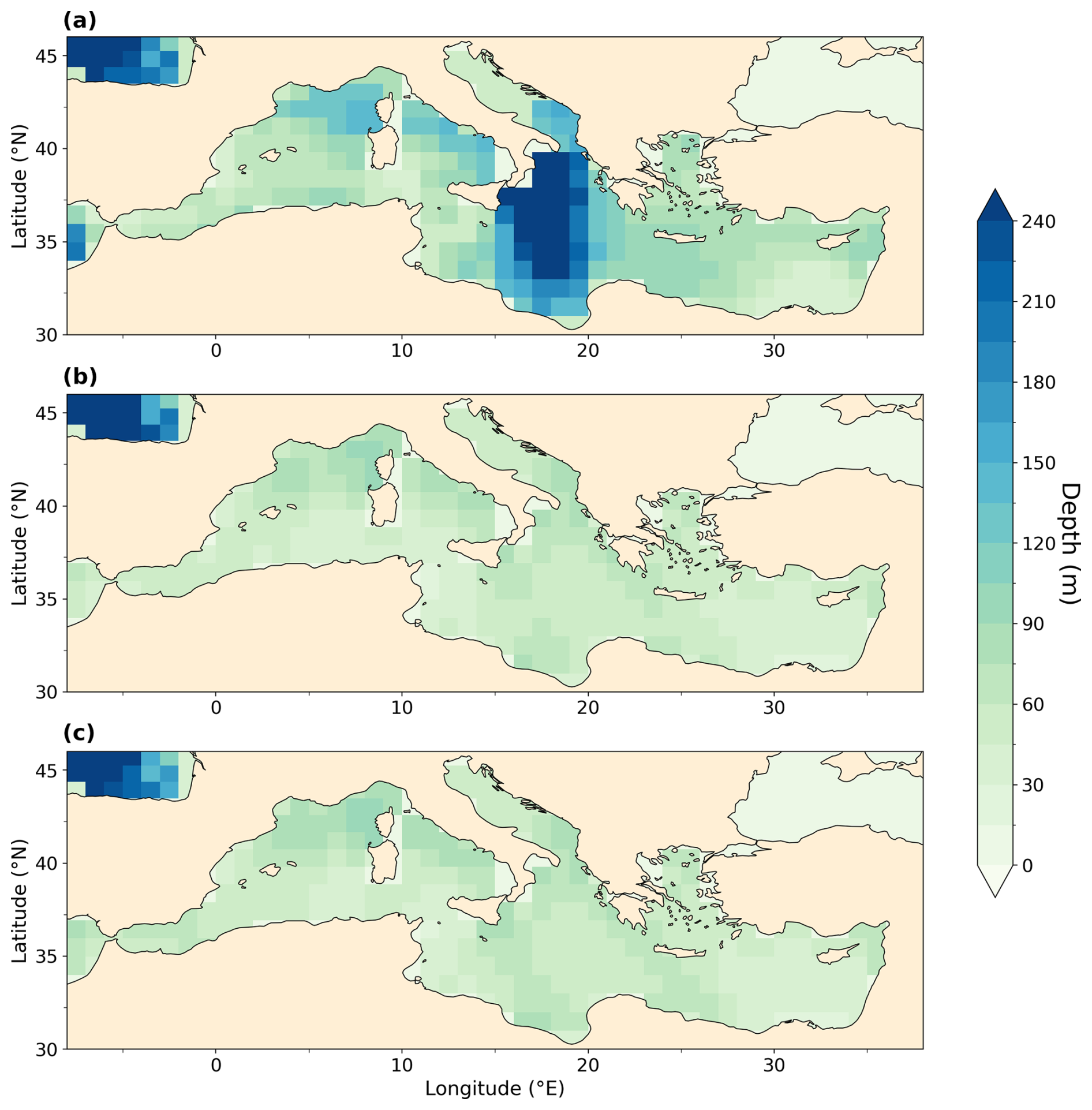
Figure A10 Mixed layer depth in the Mediterranean Sea averaged over boreal winter (DJF) in meters (m). Mean over DJF months is processed following paleo-seasonal adjustments (Bartlein and Shafer, 2019) with reference dates of 127 and 333 ka for LIG and MIS 9e, respectively. (a) PI, (b) LIG, and (c) MIS 9e.