the Creative Commons Attribution 4.0 License.
the Creative Commons Attribution 4.0 License.
 | 24 Apr 2024
An annually resolved chronology for the Mount Brown South ice cores, East Antarctica
Nerilie J. Abram
Alison S. Criscitiello
Camilla K. Crockart
Aylin DeCampo
Vincent Favier
Vasileios Gkinis
Margaret Harlan
Sarah L. Jackson
Helle A. Kjær
Chelsea A. Long
Meredith K. Nation
Christopher T. Plummer
Delia Segato
Andrea Spolaor
Paul T. Vallelonga
Climate reconstructions of the last millennium rely on networks of high-resolution and well-dated proxy records. This study presents age-at-depth data and preliminary results from the new Mount Brown South (MBS) ice cores, collected at an elevation of 2084 m on the boundary of Princess Elizabeth Land and Kaiser Wilhelm II Land in East Antarctica. We show an initial analysis of the site meteorology, mean annual chemical species concentrations and seasonal cycles, including the identification of a seasonal cycle in fluoride concentrations. The annually resolved chronologies were developed from the chemistry data using a site-specific layer-counting methodology that employed seasonally varying trace chemical species and stable water isotopic ratios, combined with alignment to known volcanic horizons. The uncertainty in the determination of annual horizons via layer counting was also quantified. The chronologies developed include the “Main” 295 m record spanning 1137 years (873–2009 CE) and three surface cores spanning the most recent 39–52 years up to the surface age at the time of drilling (austral summer 2017/2018). Mean annual trace chemical concentrations are compared to the Law Dome ice core (located 1130 km east of the Mount Brown South site) and discussed in terms of atmospheric transport. The MBS chronologies presented here – named MBS2023 – will underpin the development of new palaeoclimate records spanning the past millennium from this under-represented region of East Antarctica.
- Article
(7283 KB) - Full-text XML
- BibTeX
- EndNote


The variability of mid- to high-latitude climate over recent millennia is poorly understood in the Southern Hemisphere (Jones et al., 2016). In the Indo-Pacific sector of the Southern Ocean, data sparsity is particularly acute prior to the satellite era in 1979 due to the lack of inhabited land masses and meteorological stations. In addition, there are few millennia-scale, high resolution (seasonally to annually resolved) palaeoclimate records from ice core drilling efforts in the Indo-Pacific sector of East Antarctica (Jones et al., 2016; Stenni et al., 2017; Thomas et al., 2017, 2023). As an example, for the 100° of longitude spanning 50–150° E there is only one existing millennial-length coastal ice core record (Law Dome). This study introduces the Mount Brown South ice cores, which will add new, long, coastal ice core records to this region and contribute to global efforts to expand the network of annually resolved Antarctic ice core records spanning the last 1–2 millennia (see https://pastglobalchanges.org/science/end-aff/ipics/white-papers, last access: 15 May 2023).
This study presents the ice core age-at-depth scales (chronologies) derived from layer counting of seasonally varying chemical species and variations in stable water isotopic ratios for the Mount Brown South (MBS) “Main” ice core, an intermediate length record drilled over austral summer 2017/2018, as well as the three 20–25 m surface cores from the same drilling site and season. The MBS site was chosen after a comprehensive site selection effort that incorporated remote sensing and radar surveys across a number of promising ice core sites in East Antarctica (Vance et al., 2016). Site selection also incorporated data from a network of 30 short (5–15 m) surface cores collected across coastal East Antarctica over the last 3 decades by the Australian Antarctic Program, including in the Mount Brown region (Smith et al., 2002; Foster et al., 2006). The following seven desirable physical criteria were defined to locate multiple prospective East Antarctic sites:
-
ice of up to 2000 years age at 300 m depth,
-
no or minimal likelihood of summer melt (to aid preservation of climate signals),
-
mean annual snowfall accumulation of >0.25 m ice equivalent (to enable sub-annual sample resolution),
-
minimal local surface re-working (to maximize preservation of climate signals),
-
site location on a ridgeline or dome to reduce ice advection through time,
-
an atmospheric link to the mid-latitude circulation of the Indian Ocean,
-
a record complementary (i.e. adds new information) to the existing coastal East Antarctic ice core array.
The Mount Brown South site was identified as one of four promising regions across the 50–120° E sector of coastal East Antarctica that falls within the Australian Antarctic Program's operations region. The chronologies presented here follow two initial studies. The first is of sea salt and snowfall accumulation rates over the 1975–2017 period, which combined data from the upper portion of the intermediate length record and the three 20–25 m surface cores drilled at the Mount Brown South site (Crockart et al., 2021). The second analysed seasonal and event-scale variability in stable water isotopic ratios over the satellite era (Jackson et al., 2023). These prior studies show that for the satellite era, the new MBS ice cores fulfil the stipulations in the site selection study, albeit with a tendency toward higher annual accumulation rates than originally estimated in Vance et al. (2016).
1.1 Mount Brown South drilling site characteristics
The Mount Brown South site is located on the boundary of Princess Elizabeth Land and Wilhelm II Land, East Antarctica, at 69.111° S, 86.312° E, 2084 m a.s.l. (Fig. 1). Ice thickness in the region around the site has a mean value of approximately 2000 m. During site selection, we prioritized sites with minimal elevation change and ice advection over the last millennium (see Fig. 3 in Vance et al., 2016). Mean annual surface air temperatures (T2) for the MBS site derived from the Modèle Atmosphérique Régional (MAR) (Agosta et al., 2019) are −27.9 °C, while mean summer (DJF) surface air temperatures are −18.4 °C. The nunatak of Mount Brown is located 62 km north of the drill site, while the nearest permanently operated Antarctic station (Davis station) is 380 km to the west (Fig. 1). The ice core site is 12.6 km WSW of a 10 m surface core (“MBS99”) drilled in December 1998 (Smith et al., 2002; Foster et al., 2006). The cores described in this study are named “MBS1718” to differentiate them from past and future ice drilling at this site. For simplicity, in this study we will hereafter refer to the 2017/2018 ice cores as “MBS” unless comparing them to the earlier drilling effort.
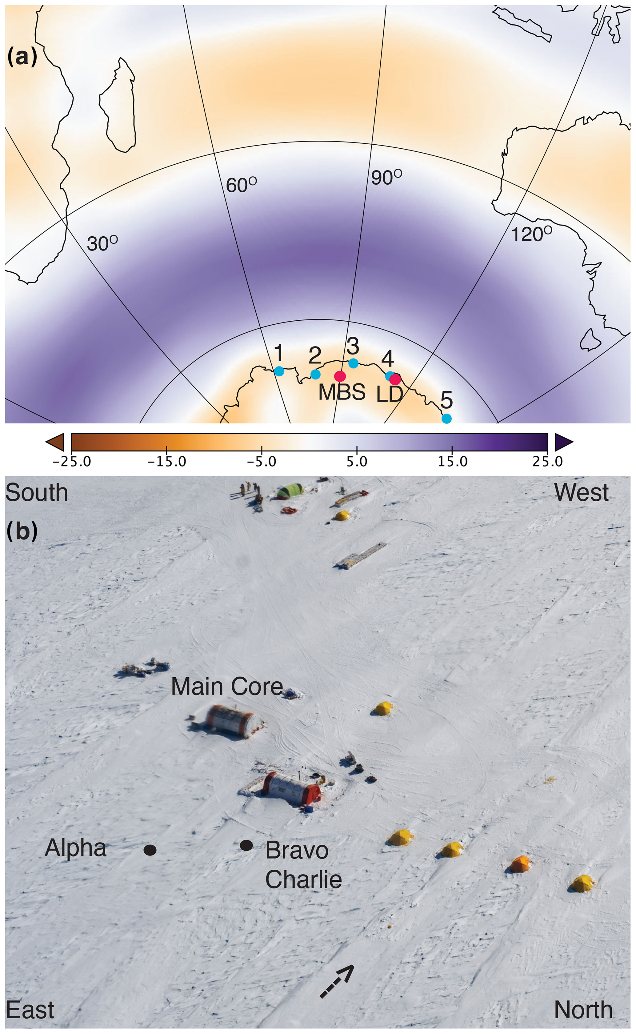
Figure 1(a) The southern Indian Ocean and East Antarctic coast with the Mount Brown South ice core drill site shown (pink dot, MBS). Indian Ocean sector mean zonal wind over the satellite era (1979–2016) indicates the prevailing mid-latitude westerly wind stream (purple shading) and the polar easterlies around the coastline of Antarctica (orange shading) in metres per second. The relative positions of the East Antarctic research stations Mawson (1), Davis (2), Mirny (3), Casey (4) and Dumont D'Urville (5) are indicated from west to east, respectively (blue dots). The Law Dome drill site is approximately 100 km east of Casey station (pink dot, LD). (b) Aerial photo of the Mount Brown South site and drilling camp showing the relative locations of the Main core (drill tent) and surface cores Alpha and Bravo/Charlie, located 94 and 82 m from the Main core and drill tent, respectively. A snow pit (data not considered in this study) was dug within 5 m of the Bravo/Charlie drill location. Large windblown surface features aligned to approximately 80° can be seen across the site, with smaller features aligned to approximately 110°, reflecting the predominant easterly airflow (note arrow at bottom of image showing predominant wind direction). See Crockart et al. (2021) and Jackson et al. (2023) for alternative site maps. Photo credit: Doug Westersund/Kenn Borek Air.
Crockart et al. (2021) and Jackson et al. (2023) found the snowfall accumulation regime at MBS to follow a seasonal cycle of higher precipitation during the polar winter (March–October) and lower precipitation during December and January. Variability between accumulation records across the site was present due to the prevailing easterlies and resulting surface features (Fig. 1), which in some cases were found to be of equivalent height to the satellite era mean annual accumulation rate of 0.3 m i.e. (ice equivalent) (Fig. 2 and Crockart et al., 2021). Coastal East Antarctica is subject to maritime moisture intrusions, which result in intense precipitation events occurring over hours to days, a subset of which reach thresholds to be classified as atmospheric rivers (Gorodetskaya et al., 2014; Turner et al., 2019; Wille et al., 2021). At MBS, intense precipitation events on average account for 44 % of annual accumulation (Jackson et al., 2023). These events are strongly related to mid-latitude blocking in the southern Indian Ocean to the northeast of MBS, which channels warm and moist maritime air masses to the site (Jackson et al., 2023; Pohl et al., 2021; Udy et al., 2021). These episodic links between East Antarctica and mid-latitude variability in the southern Indian and southwest Pacific Oceans comprise a “synoptic bridge” that leads to preservation of regional SW Pacific and subtropical climate signals in East Antarctic ice cores (Udy et al., 2022; Armstrong et al., 2020; Kiem et al., 2020).
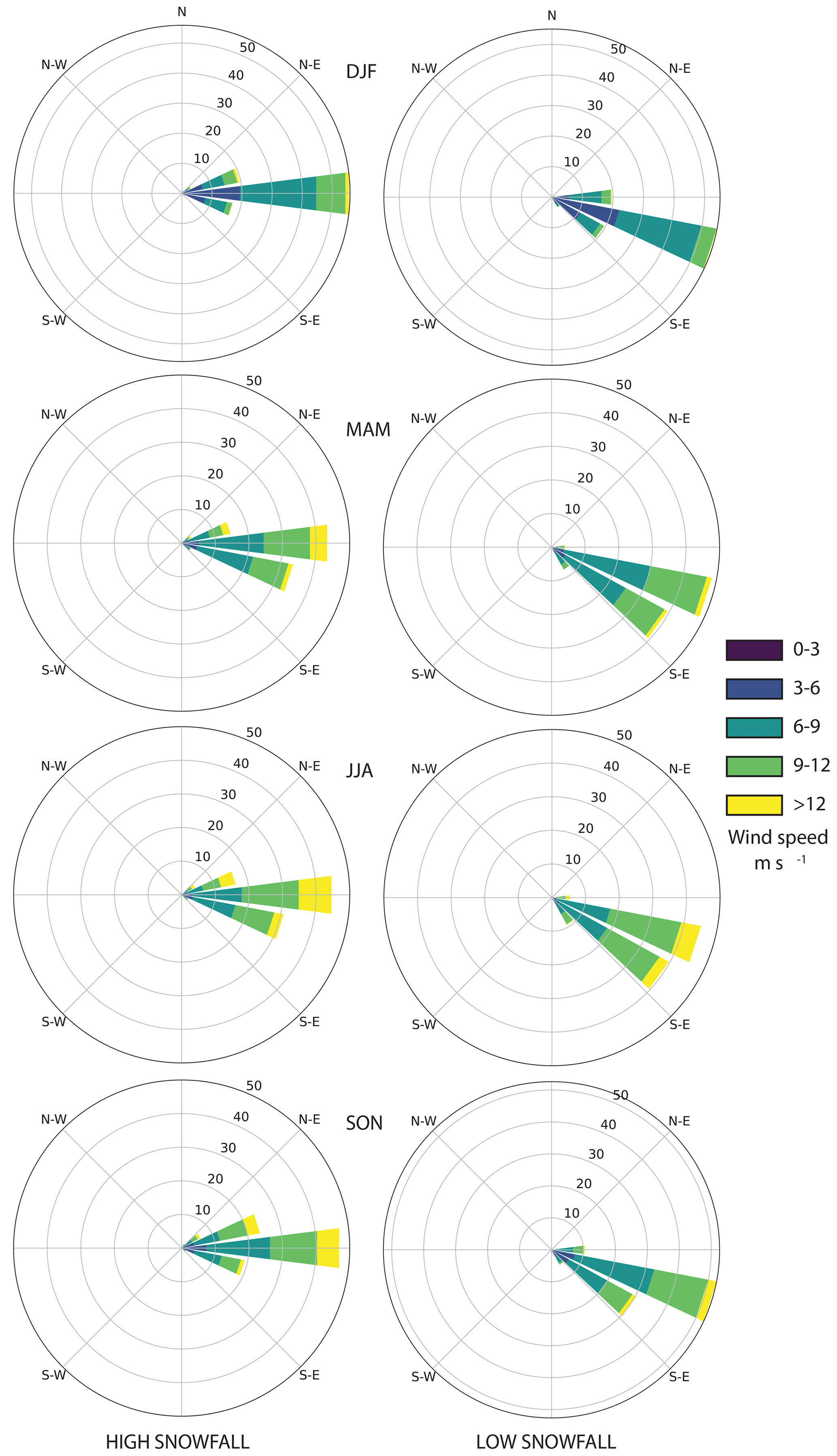
Figure 2Seasonal wind speed (m s−1), frequency (as a percentage of time) and direction at the MBS site during high (>1 mm water equivalent per day) and low (<1 mm water equivalent per day) snowfall regimes from the Modèle Atmosphérique Régional over the satellite era.
We derived estimates of site climatology from the regional climate model, MAR, for the nearest pixel to the MBS drilling site (69.2429° S, 86.4785° E, 2138 m a.s.l.). Only limited variability in prevailing wind speeds and directions occurs during each season. Slower wind speeds occur in DJF, which shows daily wind speeds only rarely exceed 12 m s−1 (Fig. 2). Higher precipitation is associated with winds directly from the east, while lower snowfall occurs when there is a southerly aspect to the easterly flow. At the time of drilling the MBS site showed numerous large surface features which were up to tens of metres wide and hundreds of metres long aligned to approximately 80° (Fig. 1 and Crockart et al., 2021). Other smaller features of a few to tens of metres crossed these larger surface features and were aligned to around 110°, suggesting wind from these directions had occurred in the weeks to months prior to drilling. Given the seasonal cycle of accumulation at MBS displays higher accumulation during the polar winter (March/April to November), this suggests a relationship between accumulation and wind speed. For a deeper analysis of variability in water isotopic ratios, temperature, and wind direction, see Jackson et al. (2023). No particular differences in wind speed and direction were observed between different reanalysis products (e.g. MAR versus ERA 5) or from 1 decade to the next.
2.1 Drilling and field processing
The MBS Main core and the three surface cores, Alpha, Bravo and Charlie, were drilled over 4 weeks in austral summer 2017/2018 (Table 1). A 1.87 m deep snow pit was also excavated, located within 5 m of the Bravo and Charlie surface cores. Snow pit temperatures were taken every 5 cm and ranged between −15 and −24.7 °C.
Table 1Description and locations of the four Mount Brown South ice cores. MBS Alpha, Bravo and Charlie were drilled using a Kovacs surface core system. The MBS Main core was drilled using a Hans Tausen intermediate-depth system.
MBS Main was drilled using the Hans Tausen drill (Johnsen et al., 2007; Sheldon et al., 2014a) from 4.25 m below the surface to the end of drilling at 294.785 m. At 93.6 m depth, wet drilling commenced with the use of ESTISOL 140 as drilling fluid (Sheldon et al., 2014b; Talalay et al., 2014). The three shallow cores were drilled using a Kovacs Mark II ice core drill coupled with a battery-powered electric motor. After drilling, each core sample was cut into 1 m lengths using a handsaw, and the length, diameter and weight were recorded for density calculations before storing in sealed polyethylene (LDPE) bags. Core samples were stored in insulated boxes beneath the snow surface to keep frozen until being flown to freezer storage at Davis Station and then transported by ship to Australia.
2.2 Core processing and sample preparation
Core sectioning and discrete sample preparation occurred in the −18 °C ice core processing freezer laboratories at the Institute for Marine & Antarctic Studies (IMAS) in Hobart. Here, detailed records and drawings, including dimensions, breaks, drilling and transport damage, wind crusts, and other stratigraphic features were made. The cores were then sectioned using a cleaned bandsaw installed in our ice core freezer laboratory according to a planned cutting guide (Fig. 3). Two 34×34 mm ice sticks were taken along the length of the Main core for trace ion analysis: one for discrete trace ion chromatography and one for continuous flow analysis (CFA). Both CFA and discrete chemistry sticks were sectioned from the Charlie core as well, and a discrete chemistry stick and isotopes strip were taken from the Alpha core. A surface strip for isotope analysis was sectioned from the Bravo core, with the remainder preserved for persistent organic pollutant studies. Prior analysis of the Alpha and Bravo cores (which were drilled in close proximity) has shown they have very similar isotope records (Crockart et al., 2021) meaning the age-by-depth scale developed for the Alpha core can be easily mapped to the persistent organic pollutant records that will be developed from the Bravo core.
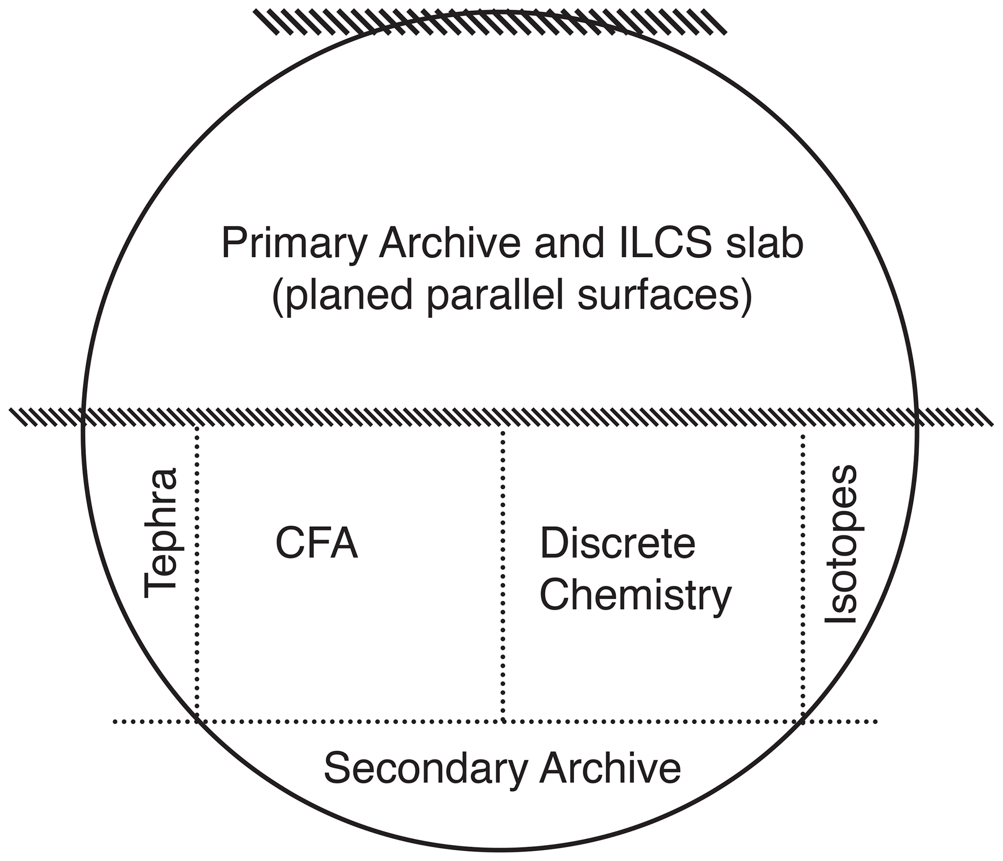
Figure 3Sampling schematic for the primary analyses of the Mount Brown South Main ice core. The core had a nominal diameter of 98 mm, and the CFA and discrete chemistry sticks were cut at a nominal size of 34×34 mm. Dotted lines indicate processing via bandsaw, while dashed lines indicate planed surfaces of the remaining primary archive prior to imaging via an intermediate-layer ice core scanner (ILCS). CFA indicates the analysis stick for continuous flow analysis at the University of Copenhagen. The remaining primary and secondary archive sections have been stored under clean and low-temperature conditions for future analyses.
Discrete trace chemistry samples at 3 cm resolution were produced under laminar flow in an ice core freezer using the clean procedures outlined in Plummer et al. (2012), Sanz Rodriguez et al. (2019) and Crockart et al. (2021). For a standard bag length, the final discrete sample of a 1 m ice core was subsequently 4 cm (isotopes) or 3.5 cm (discrete chemistry), yielding 33 samples per bag (metre) of ice. The slightly shorter discrete chemistry final sample length resulted from the sample cleaning technique, which utilized a vice in a laminar flow hood to restrain the chemistry stick during sample preparation, which resulted in a small remaining portion (typically 0.5 cm) in the vice. Given the accumulation rates calculated for the satellite era in Crockart et al. (2021), this sampling resolution yields a mean discrete sample resolution of 10 samples per year in the ice sections of the MBS record and a mean of 15 samples per year in the firn. We also used proven sample melt–refreeze procedures to preserve methanesulfonic acid concentrations in sample meltwater prior to analysis (Abram et al., 2008; Roberts et al., 2009).
Discrete water isotope samples were sectioned at a resolution of 3 cm, except between 17–35 m of the Main core where samples were taken at 1.5 cm resolution in order to investigate optimal sampling resolution for identifying annual layer horizons. Interlaboratory comparison and calibrations (Jackson et al., 2023) identified that sufficient temporal resolution for annual layer counting was obtained by 3 cm sectioning.
2.3 Trace chemistry and stable water isotope analysis from discrete samples
Trace analyses of chloride (Cl−), nitrate (), sulfate (), methanesulfonic acid (MSA−), fluoride (F−), sodium (Na+), magnesium (Mg2+), calcium (Ca2+) and potassium (K+) were made on the 3 cm discrete samples using suppressed ion chromatography. For detailed methods of discrete analysis, see Jong et al. (2022), and references therein. In brief, we used an Ionpac CS19 (Thermo ScientificTM/DionexTM) cation analytical column to improve detection and separation of magnesium and calcium peaks (Plummer et al., 2012) and an Ionpac AS15 anion column, which greatly improved separation of fluoride and MSA over previous methods and columns (Sanz Rodriguez et al., 2019). During analysis we noticed that the MSA data between 20–93 m of the Main core exhibited unknown contamination affecting peak detection. This organic contamination only affected separation of MSA. An additional 34×32 mm ice stick for this section was prepared for reanalysis, including 5 m of overlap (i.e. 15–93 m) to ensure sample reproducibility.
An additional time series of interest for dating and alignment with volcanic horizons – the sulfate-to-chloride ratio – was derived from the raw trace chemistry data. This ratio produces a clear annual boundary at the MBS site, similar to at Law Dome (Plummer et al., 2012; Jong et al., 2022; Crockart et al., 2021).
Identification of known pre-historical volcanic events is crucial to the analysis of error in layer-counted ice core records. Given the three primary sources of to the Antarctic ice sheet (sea salt aerosol, biogenic activity and volcanic eruptions), we identified volcanic events by estimating the non-sea-salt component of (nss) according to Plummer et al. (2012). We calculated a relative estimate of nss (Eq. 1) using the seawater ratio (R) of total to Na+ concentrations to remove the bulk sea salt component. Note that our analytical outputs are in µEq L−1, and thus R=0.1201.
Importantly, this relative estimate does not quantitatively calculate of volcanic origin at MBS. To do this, we would need to remove the seasonal cycle (in order to estimate and remove the biogenic component) and also account for any local or regional fractionation of the sea salt signal (for example, due to depletion from the formation of frost flowers on sea ice). This fractionation would vary the value of R slightly (see Plummer et al., 2012, and Palmer et al., 2002, for this fractionation estimate at Law Dome) but is unnecessary for the identification of volcanic peaks in this study.
We undertook sequential interlaboratory comparisons of discrete and CFA-derived stable water isotopic ratios at the three water-isotope-capable laboratories involved in this study – AAPP/IMAS in Hobart, Australia; the Australian National University in Canberra, Australia; and the Centre for the Physics of Ice, Climate, and Earth at the Niels Bohr Institute (University of Copenhagen) in Copenhagen, Denmark. For the upper 73 m of the Main core and all surface cores, the water isotopic ratios of δ18O and δD were analysed as discrete samples by cavity ring-down spectroscopy on a Picarro L2130-i water isotope analyser in Hobart. Then, discrete Main core samples from the top to 110 m depth and the Charlie surface core (which included those samples already analysed in Hobart) were shipped to Canberra and were analysed for δ18O, δ17O and δD on a Picarro L2140-i water isotope analyser. These samples provide a large analytical interlaboratory comparison between the Hobart and Canberra laboratories, as well as a 16 m interlaboratory comparison with CFA isotope data analysed in Copenhagen. See Table 2 for details of the water isotope analyses undertaken by depth and laboratory. Jackson et al. (2023) report excellent interlaboratory agreement (r>0.99 for all parameters), suggesting negligible fractionation between melt and refreeze episodes of samples or interlaboratory differences between the various analysis campaigns. A manuscript detailing the full isotope dataset is under preparation.
Table 2Details of sampling and analyses for stable water isotopic ratios over the three laboratories involved in this study, including the overlapping sections allowing interlaboratory and analytical comparisons.
2.4 Continuous flow analysis of trace chemistry, hydrogen peroxide, dust and stable water isotopes
Sample sticks (34×34 mm) for continuous flow analysis (CFA) sectioned from the MBS Main core and the Charlie surface core were shipped frozen to Copenhagen to be analysed via CFA at the Niels Bohr Institute (Kaufmann et al., 2008; Bigler et al., 2011). We used a modified version of the Copenhagen CFA system (Bigler et al., 2011; Kjær et al., 2022) during two campaigns, where the first analysed the dry-drilled sections of the Main core (4–93.6 m) and the Charlie core (CFA1: November 2018), while the second analysed the deeper wet-drilled section (93.6–295 m) of the Main core (CFA2: November 2019).
Prior to melting, sample stick ends and breaks were cleaned by removing around 1 mm of ice using a microtome blade. The cleaned ice was then placed vertically on the melt head inside a small freezer. During melting, depth registration was via a laser (2018) or a cable encoder (2019). In the 2019 campaign the sticks were melted as is. In 2018, the sticks were cut into 50 cm sections to fit the smaller holder frames. The melt head barrier (26×26 mm) ensured separation of the outer (potentially contaminated) sample stream from the inner (clean) melt stream during melting. The inner melt stream was continuously pumped through a buoyancy debubbler to remove air bubbles (see Bigler et al., 2011).
The debubbled melt stream was split into several analytical systems, including insoluble dust (Abakus), conductivity, and several simple fluorescence and absorption methods to analyse ammonium (), sodium (Na+) and calcium (Ca2+) (Bigler et al., 2011), hydrogen peroxide (H2O2), and acid (H+) (Kjær et al., 2016, 2022). Chemical signals were converted to concentrations using a linear regression produced by a set of two (H2O2 and acid) or three (, Na+ and Ca2+) known standards, and the measured flow rate was used to convert the dust concentrations from counts per second to number of particles per millilitre. Calibrations were performed before and after each sample run (approximately 4 hourly). Around 5 m (2018) or 10 m (2019) of ice was melted sequentially, prior to returning the system to ultrapure deionized water (Milli Q, 18.2 MΩ cm−1) to establish a baseline and run calibration standards. At the start and end of each sample run, system blanks of deionized ultrapure water were analysed. Melt speed was maintained at around 3 cm min−1 (2018) or 3.5 cm min−1 (2019), providing slightly higher resolution in the 2018 data. A detailed description of the CFA trace chemistry and impurities set-up and dataset is in preparation.
An additional line of debubbled water for the analysis of stable water isotopes (δ18O, δD) was included for the 2019 CFA campaign which analysed the wet drilled cores. The water isotope line was modified from the one described in Gkinis et al. (2010, 2011). Water was pumped through the system at a rate of 0.4 mL min−1, with the rate controlled by a peristaltic pump. The water sample passed through a 2 µm filter to remove any particulate matter prior to injection into an evaporation oven (set at 170 °C) via a 40 µm fused silica capillary. The evaporated sample was mixed with dry carrier air and transferred to the cavity ring-down spectroscopy (CRDS) optical cavity of a Picarro L2130-i at a humidity level of 15 000 ppm. In-house standards (calibrated to Vienna Standard Mean Ocean Water (VSMOW) and Standard Light Antarctic Precipitation (SLAP)) were used to calibrate the samples. The measurement noise as inferred by the integration of the power spectral density of the δ18O and the δD signals is 0.08 ‰ and 0.43 ‰, respectively. The mean accuracy of the record, calculated using a “check” water standard, is 0.03 ‰ and 0.3 ‰ for δ18O and δD, respectively. A detailed description of the CFA water isotope dataset is in preparation.
2.5 Inductively coupled plasma sector field mass spectrometry of sodium, calcium, iodine and bromine
Discrete subsamples were taken via a dedicated CFA line to a fraction collector every 25 cm during the Copenhagen CFA campaigns. These samples were transported frozen to the Ca' Foscari University (Venice, Italy) and stored at −20 °C. Total Na, Ca, bromine (Br) and iodine (I) concentrations were determined with an inductively coupled plasma sector field mass spectrometer (ICP-SFMS, Thermo ScientificTM ELEMENT2TM) equipped with a cyclonic spray chamber. The discrete samples were not acidified to avoid possible volatilization of I and Br during the analytical sequence. A 10 h cleaning sequence was run before the sample analytical sequence by alternating ultrapure water and a solution of 2 % ultrapure HNO3 until the blanks reached low and stable levels. I and Br analyses are susceptible to instrumental memory effects (Vallelonga et al., 2021). Given the low average concentrations determined for halogens in ice cores and the halogen memory effect, it is essential to ensure minimum background conditions between each sample analysis; thus, the ICP-SFMS was cleaned between samples by drawing 2 % HNO3 and then deionized ultrapure water for 60 s each, respectively. Flowing ultrapure water through the ICP-MS tubing before the sample analysis has two effects. First, it removes any nitrate salts that may be deposited by the nitric acid. Second, it conditions the instrument before introducing the unacidified samples.
Concentrations were calculated by comparison to both external standards and blank correction. External standards were prepared from mono-elemental solutions (TraceCert®, purity grade, Sigma-Aldrich, MO, USA) with concentration ranges of 5 to 300 ng g−1 (Na and Ca), 0.5 to 3 ng g−1 (Br) and 0.05 to 0.3 ng g−1 (I). The calibration curves showed a linear relationship and had a correlation coefficient greater than 0.99 (p value ≤ 0.05). Blanks were measured every 15 samples and the limit of detection (LOD), calculated as 3.3 times the standard deviation of the blanks, was 0.1 ng g−1 (Na), 1.1 ng g−1 (Ca), 0.05 ng g−1 (Br) and 0.002 ng g−1 (I). About 10 % of the samples were reanalysed to ensure repeatability, showing a variability of 2.1 % (Na), 4.5 % (Ca), 3.1 % (Br) and 7.7 % (I) with respect to the original measurement. The paleoenvironmental value of this dataset from the MBS site is under investigation; however, for the purposes of this study, we present the annual mean halogen concentrations at MBS compared to those from the Law Dome ice core.
2.6 Imaging of stratigraphic features via intermediate-layer core scanning (ILCS)
The MBS ice cores contain numerous stratigraphic features, particularly thin crusts. These crusts are qualitatively similar to bubble-free layers identified elsewhere in Antarctica and Greenland, and they are distinct from melt layers in appearance by being thin (1–2 mm thick) and sharply defined rather than thick and ragged in appearance. At the West Antarctic Ice Sheet (WAIS) Divide, such bubble-free layers have been determined to be unrelated to melt events via noble gas analysis (Orsi et al., 2015). The MBS bubble-free layers appear regularly, with multiple instances per annual layer. In order to investigate these features and any climate information they may hold, stratigraphic imaging of the remaining half sections of all MBS ice cores after glaciochemical sampling was undertaken using an intermediate-layer ice core scanner (ILCS, Shåfter & KirchoffTM) and image acquisition system. For the purposes of this study, the ILCS images were used to help align depths across different samples and laboratories due to depth alignment issues we encountered (see below), and thus we describe the processing of ice core slabs for ILCS image acquisition here. The climatological or physical causes of these bubble-free layers in coastal East Antarctic cores and their variability through time are currently under investigation elsewhere (Zhang et al., 2023). An example of an ILCS image of an MBS ice core used to constrain the depth scale is given in Appendix A1.
ILCS is commonly used to image ice cores for analysis or dating of dust or volcanic layers, generally in deeper ice cores drilled from below bubble close-off depths (Svensson et al., 2005; McGwire et al., 2008; Winstrup et al., 2012; Westhoff et al., 2022). The ILCS instrument consists of a frame surrounding a removable carriage that holds the polished ice core slab to be imaged. A camera mounted above the carriage and an indirect light source mounted below at an angle of 45∘ relative to the ice move synchronously from one end of the ice core slab to the other. The image acquired is a greyscale image, which reveals clear ice to be darker or black and impurities and bubbles in the ice as grey or white.
Pre-processing of the ice core surface to be scanned was necessary in order to avoid interference from surface artefacts of core processing (e.g. bandsaw blade marks). We used a modified and cleaned timber planer and thicknesser modelled on a simplified version of the set-up used at the National Science Foundation Ice Core Facility (Colorado, USA) (McGwire et al., 2008). We designed a polypropylene tray system that allowed ice core slabs of varying dimensions to be secured safely in place while passing the tray through the thicknesser. Swarf produced during planing was removed with a clean, commercial vacuum cleaner attached to the dust port of the planer. We also used clean brushes and scrapers similar to those used in our ice core processing freezer to remove any particles of ice or dust remaining after planing that would interfere with image acquisition.
Once planed and microtomed to a smooth surface, the core slabs were left overnight to sublimate slightly, which allowed a polished surface to develop. Each core slab was then scanned multiple times at different focus heights and brightness settings to ensure optimum image quality. We also used multiple changes in focus heights and brightness settings to acquire images of firn cores that would preserve features such as bubble-free layers and crusts in shallower records (Zhang et al., 2023).
2.7 Constructing the MBS depth model
Ideally, the top and bottom depths and individual lengths of ice cores align perfectly to those measured during drilling, yielding insignificant discrepancies between core and sample lengths between laboratories or sampling campaigns. In reality this is not always the case. We found instances where the length of MBS cores and sticks during sample cutting and pre-processing for analysis were different to the field camp lengths. Mostly this appeared due to slanted core ends (see Appendix A1) from imperfect cuts during field processing, as only hand saws were available for post-drilling processing. Additionally, two transport boxes containing MBS Main cores (12 m of ice) experienced major damage during transit from the field site to the Hobart laboratories. These broken cores were difficult to re-assemble, and in one instance this resulted in a length discrepancy of 1.5 cm. Overall, discrepancies between field and laboratory core lengths were usually less than 0.5 cm, but in rare cases they were up to 1.0 cm or even 1.5 cm. Note that these field-to-lab discrepancies are similar to those found in other ice core studies, for example, Erhardt et al. (2022). Where discrepancies in individual core or stick lengths were found, the difference between the laboratory and final accepted lengths was averaged across the sample depths within that core. This approach avoids having the uncertainty accumulate at the bottom of each core, creating an artificial gap between cores.
To solve the length discrepancies and derive a master depth model, we compared field and lab measurements to the ILCS scans to derive the correct length of each core. This painstaking process was then used to determine the full drilled depth of 294.785 m, which is 18.5 cm different from the field measured depth of 294.6 m (i.e. a 0.003 % error). This suggests that despite the discrepancies between field and laboratory measurements, the ultimate depth of the core was measured accurately and individual core discrepancies will have limited impact on sample depth registration. For the CFA analysis of trace impurities and water isotopes, a process of scaling and shift factors is being derived to account for length discrepancies. This was necessary as the length of the CFA analysis sticks sent to the University of Copenhagen were sometimes shorter or longer (by up to 0.5 cm) than the lengths of the original cores, depending on their orientation to any slanted end cuts in the whole core. The scaling and shift factors will be described in detail as the CFA trace chemistry and water isotope datasets are developed and published. For the discrete analyses used for the dating study described here, the depth model derived has been applied to each sample.
2.8 Dating the Mount Brown South Main ice core
We followed an independent plus final consensus approach to dating using the seasonally varying concentrations of multiple trace chemical species and water isotopes for identification of annual layers. An initial study of the satellite era of the MBS Main and surface cores identified that annual horizons adjacent to low-accumulation years could be difficult to detect due to truncated or unclear seasonal cycles, a finding that was reinforced by comparison with modelled precipitation and surface mass balance data for the MBS site (see Fig. 2, Crockart et al., 2021). With this in mind, we developed a methodology to produce the MBS Main core chronology and revisit the age-by-depth chronologies derived for the surface cores and satellite era portion of the Main core, as well as quantifying uncertainty from difficult to detect annual horizons through time.
A “working” age-by-depth scale (hereafter MBSCP) was developed using a layer counting approach similar to that derived for Law Dome (Jong et al., 2022; Vance et al., 2022; Roberts et al., 2015; Plummer et al., 2012). MBSCP relied on sea salt minima, isotope maxima, nss maxima and the summer peak in the sulfate-to-chloride ratio to identify annual horizons, which were assigned a date of 1 January as per Crockart et al. (2021). This is different to Law Dome, where multiple analyses using co-located automatic weather station data compared to ice core isotope records have determined the annual horizon to have a mean date of 10 January (van Ommen and Morgan, 1997; Jong et al., 2022). Constraining the mean date of the annual horizon to this degree is unusual because it requires relatively high and uniform annual accumulation rates and long-term co-located meteorological instrumentation at the site, which is not currently possible at MBS. However, we wish to remind future users of both the MBS and Law Dome records of the difference in the actual date signified by the annual horizons in both records. Preliminary alignment to known volcanic ties for Antarctic ice cores was also undertaken via comparison of nss peak occurrence, shape and relative concentration.
In parallel with the development of MBSCP, a layer-counted-only age-by-depth scale – MBSHK – was produced without reference to MBSCP by a separate investigator on this project. MBSHK used similar species to determine annual horizons to MBSCP with the following clear difference: this investigator identified a possible minimum in fluoride concentrations adjacent to the annual horizon of other species and hypothesized fluoride at MBS may follow a seasonal cycle. The investigator deriving MBSHK did not attempt to locate or incorporate known volcanic age ties, in order to deliberately derive a layer-counted-only age scale that could be used to assess how frequently annual layers were “missed” due to either a different dating approach and/or poor seasonality. Both these interim age scales defined three types of annual layers – certain years, uncertain but counted years (where there is deemed to be an annual horizon but its exact placement is uncertain), and uncertain uncounted years (where there is some evidence for an annual horizon but not enough to include as a counted year in the chronology).
We then formed the MBS dating team (comprising the bulk of the authorship of this study) to incorporate the interim age scales toward a final chronology. We examined MBSCP and MBSHK on the same depth scale (see Appendix B1 for an example section). If MBSCP and MBSHK showed agreement on annual horizons, no change was made. Where horizons differed in number or position, the final decision of annual horizon placement was made by group consensus and applied to MBSCP. Finally, the group consensus version of MBSCP was synchronized to the West Antarctic Ice Sheet (WAIS) Divide WD2014 chronology (WD2014) (Sigl et al., 2016) to produce the chronology described here – MBS2023. In MBS2023, uncertain years are defined as counted or uncounted as above. See Appendix C for a summary of the steps followed.
3.1 MBS2023 – a layer-counted chronology for the MBS ice cores
Our dating approach allowed for the comparison of independent plus consensus efforts by researchers skilled in dating ice cores from Antarctica and Greenland and incorporated a range of experience in the final group assessment of annual horizon category and placement. In addition, we re-examined the dating for the satellite era portion of Main and of Alpha, Bravo and Charlie from Crockart et al. (2021). This re-examination did not result in any changes to the original dating, and thus the analytical time series and findings detailed in Crockart et al. (2021) and Jackson et al. (2023) remain current and are upheld. The time periods covered by the three surface cores are 1977–2017 (Alpha), 1978–2017 (Bravo) and 1965–2017 (Charlie).
For MBS Main, we found the 4.265–294.785 m deep record spanned 873–2009 CE (1137 years), fulfilling the stipulations of the site selection of a millennium-length record. For the majority of MBS Main, annual horizons were relatively easy to discern, but there were periods where seasonal cycles were less pronounced and it was more difficult to define the number or placement of annual horizons. In total, we found 1004 annual horizons to be certain counted years (i.e. the dating team deemed both the evidence pointing to the existence of an annual horizon as well as its exact placement on the depth scale to be unequivocal). The remaining 133 horizons (11.7 %) were uncertain counted years. Finally, we also found 73 instances across the Main record of what we deemed uncertain uncounted years, where there was only partial evidence of an annual horizon. An example would be a minimum in sea salt concentrations that was not matched by a corresponding peak in either isotopes or the sulfate-to-chloride ratio. To reiterate, an uncertain “counted” year constitutes the definite existence of a year, but it is unclear exactly where the annual horizon signifying 1 January should be placed, while an uncertain “uncounted” year constitutes incomplete evidence for a year that is not compelling enough to be included in the chronology. In the former case of uncertain counted years, the annual horizon was placed where the dating team deemed the most evidence for its placement to be.
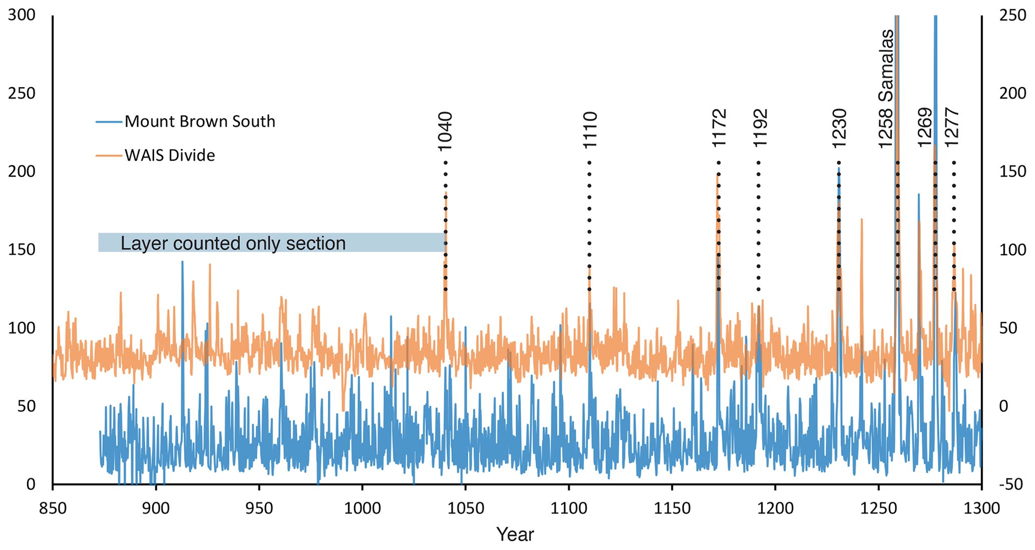
Figure 4The nss record (ppb, left axis) from the deepest third of the MBS Main core (202.4–294.6 m) synchronized to the WAIS Divide non-sea salt sulfur record (ppb, right axis, offset for visual clarity) showing volcanic tie points used to synchronize WAIS Divide and MBS. Refer to Table 3 for the full list of tie points used for synchronization and comparison. The end of the synchronized chronology and commencement of the layer-counted-only chronology for the MBS Main record at 1040 CE to the bottom of the core is indicated.
As with other more coastal Antarctic ice core records, volcanic horizons in the MBS ice core (deviations from the nss background) can be noisier signals compared to inland records due to the dilution of the signal in coastal regions (Plummer et al., 2012). Despite this, the volcanic age ties we identified were clear enough to be very useful in evaluating the uncertainty that unclear annual horizons introduces to the MBS2023 chronology (Table 3 and Fig. 4). We compared and contrasted the likely volcanic signals we discerned in the chemistry record to those of Law Dome (1377 m a.s.l., lower elevation than MBS) (Jong et al., 2022) and the Roosevelt Island Ice Core (79.36° S, 161.71° W, 550 m a.s.l., lower elevation than both Law Dome and MBS) (Winstrup et al., 2019). We also tied the MBS record to the established West Antarctic Ice Sheet (WAIS) Divide chronology, WD2014 (Sigl et al., 2016). Of note is the higher number of matched volcanic horizons in MBS to both the WAIS Divide and Law Dome records compared to the Roosevelt Island record. As Roosevelt Island is a much lower elevation record, the influence of biogenic sulfur made identifying small or short lived volcanic events difficult, leading to fewer matched horizons (Winstrup et al., 2019). Below 256.46 m depth (1040 CE), the MBS2023 chronology is based on layer-counted-only data and not synchronized to WD2014 due to the lack of an identifiable volcanic horizon below this point.
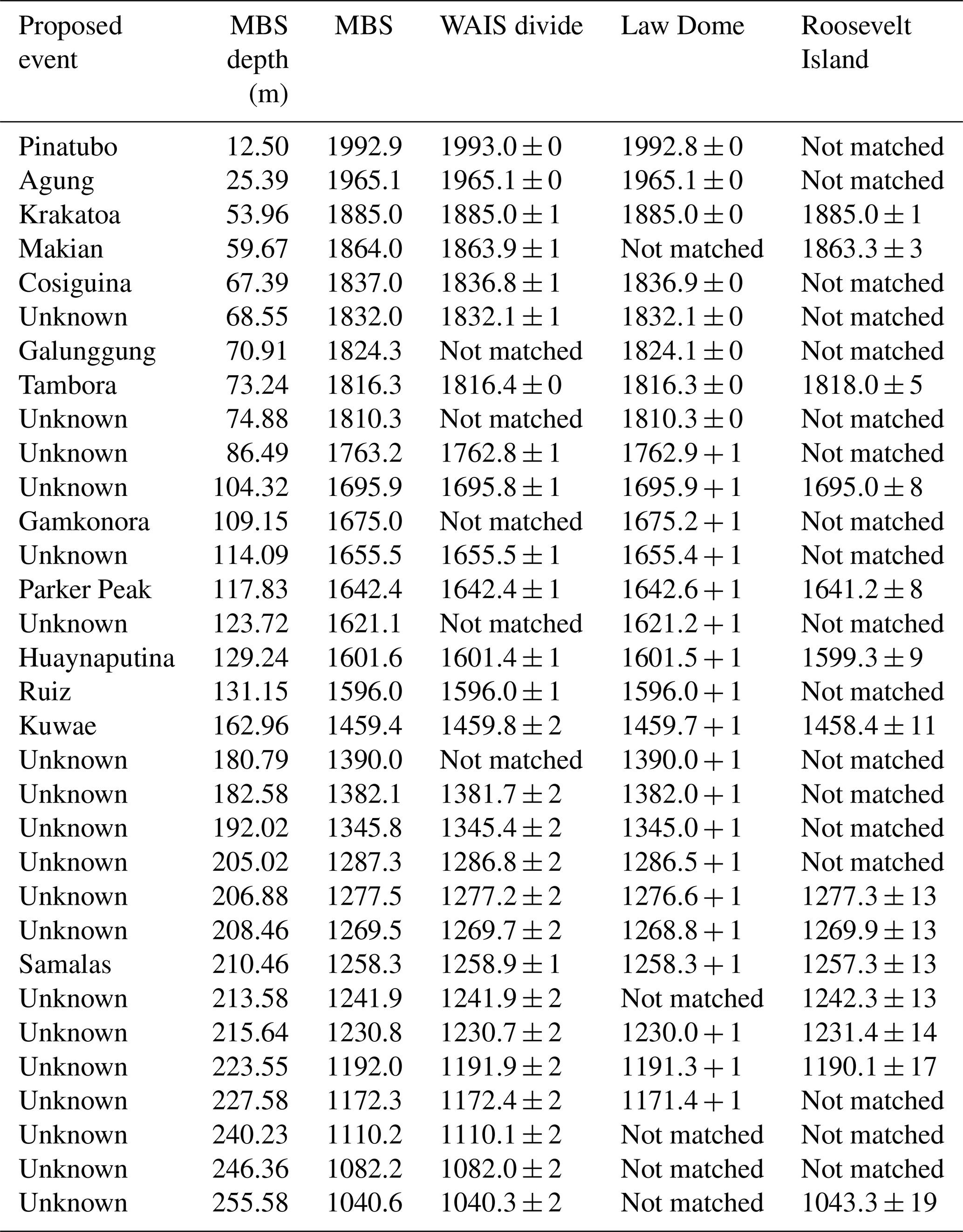
Table 3Proposed volcanic dates and depths from the MBS ice core. The MBS record has been synchronized to the WAIS Divide chronology, WD2014 (Sigl et al., 2016) at the year level, and thus WD2014 errors should be taken into account. Note however, intra-year synchronization has not been performed to illustrate differences in the onset of the volcanic signal. Comparisons with Law Dome (Plummer et al., 2012; Jong et al., 2022) and Roosevelt Island (Winstrup et al., 2019) are also shown. Note the Kuwae date may be disputed depending on which peak is matched in the 1450s (see Plummer et al., 2012); however, this is the equivalent peak matched by peak size.
3.2 Mean annual concentrations and seasonal cycles of key trace chemical species
Mean annual concentrations of key trace chemical species at MBS are generally lower than those reported from Law Dome, except for nitrate and methanesulfonic acid (Table 4). We also examined seasonal cycles for sodium, non-sea-salt sulfate, the sulfate-to-chloride ratio and fluoride (Fig. 5). As is commonly reported, this type of analysis is reliant on an assumption of uniform accumulation through the year at the site due to the lack of within-year dating markers (Winstrup et al., 2019; Kjær et al., 2022). Uniform accumulation has been shown to be not realistic (e.g. Turner et al., 2019), and we know the MBS ice core site has a precipitation bias with lower summer accumulation during the satellite era, as well as episodic inputs of precipitation that comprise a significant proportion of the annual accumulation (Crockart et al., 2021; Jackson et al., 2023). Nonetheless, seasonal cycle analysis is useful for examining the relative mean timing of minima and maxima between individual species at a given ice core site.
Table 4Mean annual concentrations of trace chemical species from the MBS Main core from 873–2009 CE compared to the Law Dome ice core from 1–2017 CE (Jong et al., 2022) except for methanesulfonic acid (1750–1995 CE) (Curran et al., 2003), total bromine, iodine, sodium and calcium (1927–1989 CE) (Vallelonga et al., 2017). The fluoride mean concentration at MBS is an interim calculation. Analytical methods for ion chromatography for the MBS analyses in this work are developed from the methods in Sanz Rodriguez et al. (2019) and Jong et al. (2022). References for the source of the Law Dome data for comparison are indicated. For specific ICP-MS methods, data validation and details around the Law Dome halogen study, see Vallelonga et al. (2017). For standard concentration ranges, mean blank concentrations and detection limits for all species, see Appendix D1.
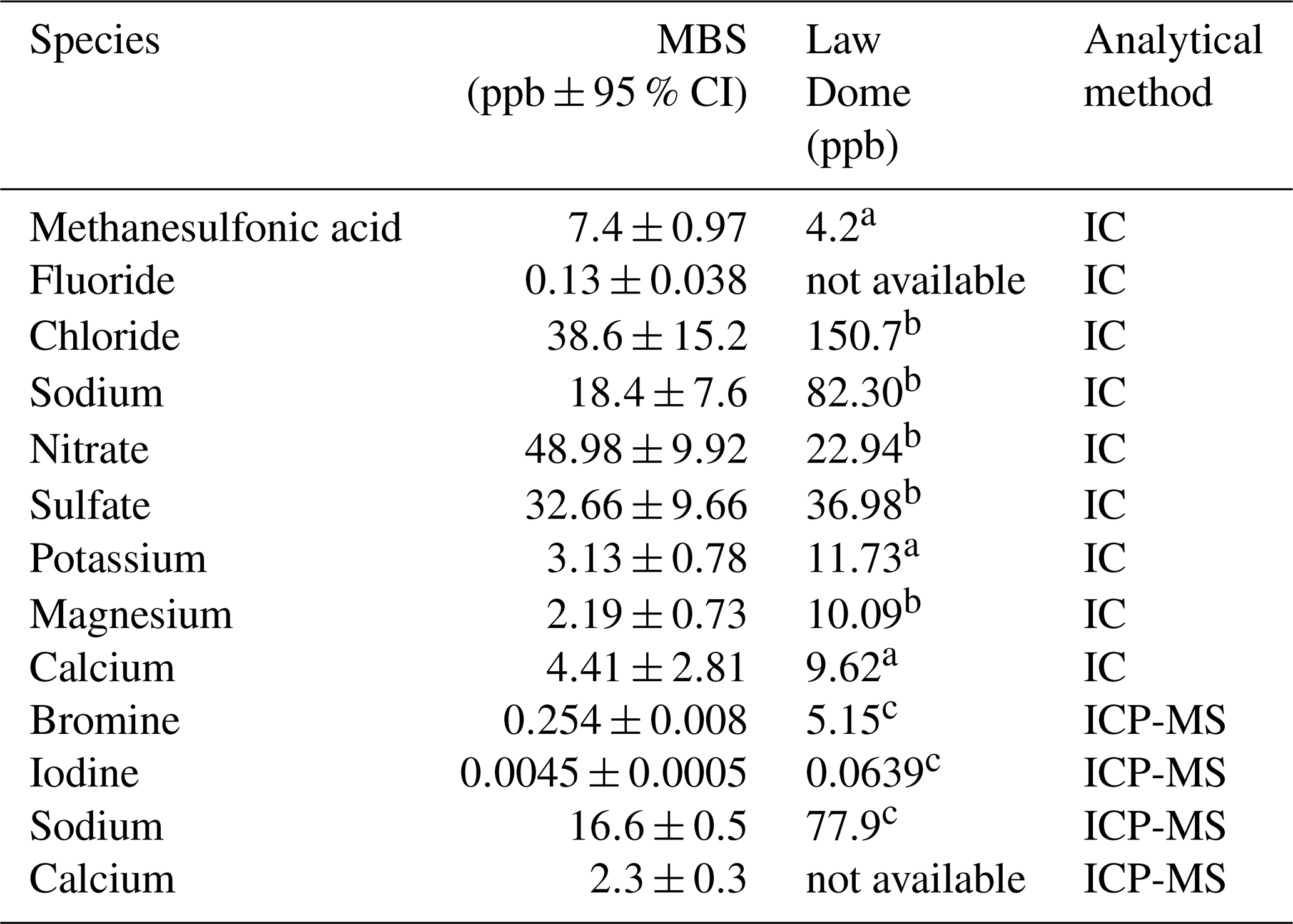
a Curran et al. (1998). b Jong et al. (2022). c Vallelonga et al. (2017).
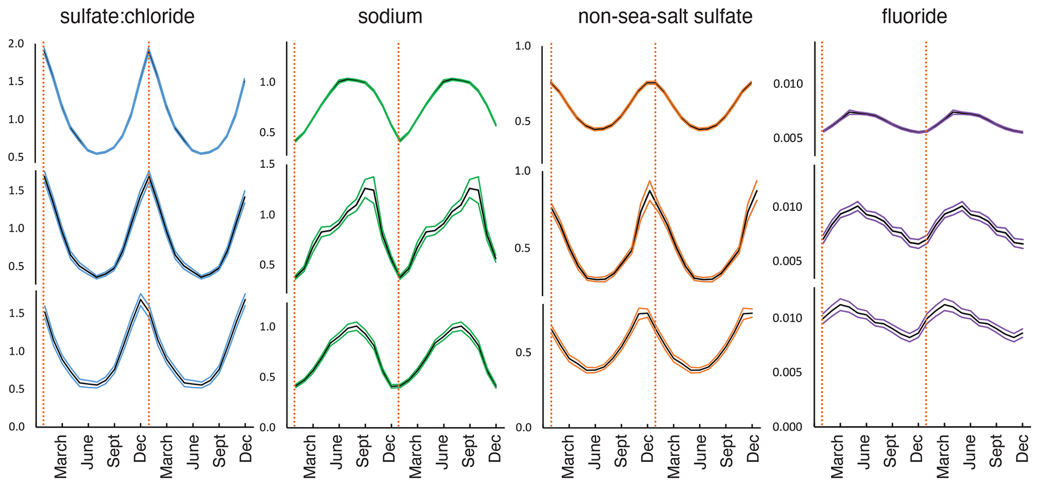
Figure 5Seasonal cycles of key trace chemical species in the MBS ice cores. Shown are seasonal cycles for the Main core during the non-satellite era (top row, 872–1978 CE), the Main core satellite era (middle row, 1978–2008 CE) and the Charlie surface core (bottom row, 1966–2017 CE). For fluoride, seasonal cycles were calculated over 962–1798 CE (Main non-satellite era, top row), 1978–2008 (Main satellite era, middle row) and 1966–2012 (Charlie, bottom row) due to the incomplete dataset available.The sulfate-to-chloride ratio (blue), sodium (green) and non-sea-salt sulfate (orange) concentrations were the primary indicators of annual layers, with fluoride (purple) being a confirmatory species. Concentrations are shown in the units used during layer counting (µEq L−1). The black line in each panel represents the mean value for that month for the time period selected, assuming uniform accumulation. The coloured upper and lower bands are the standard error of the mean. For orientation, vertical dotted orange lines indicate the annual horizon date of 1 January. For detailed analysis of stable water isotope ratios, their relationship to seasonality and the influence of biases due to moisture intrusions, see Jackson et al. (2023).
The MBS fluoride record presented here is an interim dataset, with some missing sections due to variability resulting from the very low concentrations present at MBS and possible losses in the firn section during storage. We present fluoride seasonal cycles covering time periods of adequate sample fidelity from the MBS Main and Charlie cores (Fig. 5). These show that fluoride has a minimum in early summer (November–December) and an autumn maximum (March–April–May). Note that the satellite era fluoride seasonal cycle was derived without reference to fluoride as an indicator of an annual horizon, as the satellite era age scales were developed in Crockart et al. (2021) prior to examination of the fluoride record.
We present chronologies for a new multi-century ice core and three surface ice cores from the boundary of Wilhelm II Land and Princess Elizabeth Land in East Antarctica. The ice core site – Mount Brown South – was drilled in 2017/2018 and spans 873–2009 CE and up to 2017 CE with the inclusion of the surface cores. The chronologies developed here – collectively named MBS2023 – incorporate expertise from an international team with experience in dating both Antarctic and Greenland ice cores.
4.1 Seasonal cycles of trace chemical species and the potential of fluoride as a climate proxy at Mount Brown South
The MBS records display clear seasonality in three primary analytes that are frequently used for layer counting – sea salts (principally sodium and chloride), non-sea-salt-sulfate and the ratio of sulfate to chloride (Fig. 5). Seasonal cycles of sea salt and non-sea salt sulfate exhibit expected maxima in winter (June–September) and summer (December–February), respectively, leading to a summer peak in the ratio of sulfate to chloride. We define the MBS annual horizon to have a nominal date of 1 January in accordance with Crockart et al. (2021). The installation of automatic weather stations at an ice core site over multiple years (as is the case at the Law Dome ice core site) can constrain the mean date of the annual horizon in a site-specific way (see van Ommen and Morgan, 1997). This would be difficult to achieve at MBS given the lack of co-located instrumentation and the more episodic accumulation regime, along with lower accumulation occurring in summer (Crockart et al., 2021). Some evidence that a precise annual horizon date (similar to that derived for Law Dome) would be harder to constrain at Mount Brown is the slight differences in the annual horizon peak shapes in the Charlie surface core compared to the Main core (Fig. 5).
Fluoride is an infrequently investigated species in polar ice core studies; however, it has been known to comprise part of the trace chemistry suite of Antarctic ice cores for some time (Severi et al., 2014; Morganti et al., 2007). It is usually present in low concentrations and has been shown to have multiple sources, including anthropogenic production, sea salts, volcanoes, dust and perhaps forest fires (De Angelis and Legrand, 1994; Preunkert et al., 2001). This study shows fluoride varies seasonally at MBS with a peak in austral autumn. We derived fluoride seasonal cycles for both the satellite era and in the pre-instrumental era (noting there are significant data gaps in the fluoride record). The satellite era layer counting of the Main and Charlie cores was derived without reference to fluoride as a potentially seasonally varying species (as these sections were dated prior to any investigation of fluoride seasonality, and their ages at depth are unchanged in this study). The similarity in seasonal cycle shape between the pre-instrumental era in MBS Main compared to the satellite era periods of MBS Main and Charlie suggests a robust seasonal cycle is present.
Fluoride peaks in March–April–May (austral autumn) at MBS, coincident with neither sea salt sodium that peaks later in winter (June–September) nor non-sea salt sulfate that peaks in summer (probably related to algal blooms and production of dimethylsulfide) (Trevena and Jones, 2006). Thus, fluoride at MBS seems related to neither sea salt aerosol deposition nor biogenic activity. The fluoride minimum occurs during early summer (November–December) before the sea salt minimum in January and approximately 1 month prior to the peak in the sulfate-to-chloride ratio, providing a potentially independent marker of the onset of summer at the MBS site.
We are unaware of any established regional anthropogenic, forest fire or volcanic sources that would lead to the fluoride seasonality observed at MBS. This leaves only two possible sources from the literature. Fluoride could be deposited as part of the dust fraction at MBS (presumably from the Vestfold Hills, the only regional ice-free area that could provide a dust source of any magnitude). There could alternatively be a solar-driven loss cycle to the sea salt fraction from mid-winter (however, the early maxima in March or April makes this hypothesis unlikely based on seasonal cycle shape). A third possibility that has not been canvassed in the literature but that should be investigated based on the shape and timing of the seasonal cycle is that there is a relationship between fluoride deposition and sea ice seasonality, given Antarctic sea ice retreats to its minimum extent in February–March (Raphael and Handcock, 2022). The autumn peak in fluoride could suggest a source related specifically to sea ice formation and production (which may or may not be related to maximum extent). The fluoride seasonal cycle at MBS displays an asymmetry analogous to that of Antarctic sea ice, which has a 7-month growth phase and a 5-month decline phase (Eayrs et al., 2019; Roach et al., 2022). However, establishing a relationship to sea ice formation would require investigating and disentangling any regional dust sources such as the Vestfold Hills. In addition, a closer examination of other known sea ice proxies (e.g. MSA and halogens) at MBS is warranted.
Finally, while the seasonality of the fluoride record from MBS may preserve a climatological signal, its low concentrations make measurement challenging (Sanz Rodriguez et al., 2019), the reliability of the record is variable at different periods and its volatile nature means it is subject to post-depositional modification (Legrand et al., 1996). This means development and interpretation of the fluoride record will need to incorporate possible competing sources in the MBS and East Antarctic region and quantitative analysis of pre- and post-depositional processes in the atmosphere and snow surface.
4.2 Annual mean concentrations of trace chemical species
The mean annual concentrations of the sea salts sodium, chloride, potassium and magnesium at MBS occur at around a quarter of the concentrations at Law Dome (Table 3). Sea salts have short atmospheric residence times of at most a few days (Schüpbach et al., 2018), suggesting the mean trajectory of sea salt aerosol reaching MBS has a less immediate link to maritime air masses than at Law Dome, resulting in relative depletion. This suggests that while MBS is a coastal core geographically, climatologically it is a more inland site than Law Dome. The MBS site is approximately 700 m higher than Law Dome and is thus at a transition zone to plateau records. The depleted concentrations of calcium compared to Law Dome (by around 50 %) are probably similarly related to more continental trajectories occurring at MBS, although the atmospheric residence and transport times of calcium can be longer than sea salts (Schüpbach et al., 2018).
In contrast, sulfate concentrations at MBS are similar to Law Dome, while mean annual concentrations of methanesulfonic acid (MSA) are around double those of Law Dome. This may suggest higher regional production of MSA close to MBS compared to Law Dome. MBS is relatively close to the Vestfold Hills, one of the largest ice-free areas of East Antarctica with a number of field stations, including Davis station (approximately 380 km to the west). Numerous studies of coastal phytoplankton production and seasonality have been conducted at Davis station, including studies of the phytoplankton-synthesized precursor of MSA, dimethylsulfide (DMS), and its biochemical precursor dimethylsulfoniopropionate (DMSP). These studies have detailed exceptionally high seasonal concentrations of DMS and DMSP in late-season sea ice and during and after sea ice breakout (Trevena et al., 2000, 2003; Trevena and Jones, 2006). The high concentrations may be related to rapid sea ice breakout in combination with fertilization due to windblown dust from the Vestfold Hills. This would elicit rapid phytoplankton growth and the increased production of DMS and DMSP in sulfur-producing phytoplankton species (Vance et al., 2013). However, there could be another MSA source further to the northwest of MBS. Air parcel trajectory studies show that MBS is regularly “downstream” of the Kerguelen Plateau (Jackson et al., 2023), another region of episodically very high phytoplankton production (Robinson et al., 2016; Schallenberg et al., 2018). The high concentrations of MSA at the MBS site in combination with the prior study of an earlier MBS short core investigating MSA as a sea ice proxy (Foster et al., 2006) are promising for the development of new sea ice reconstructions from the MBS ice cores (Curran et al., 2003).
The halogens bromine and iodine show far lower concentrations at MBS with respect to Law Dome over the 20th century (Vallelonga et al., 2017). On average, bromine and iodine levels are at least 20 times lower with respect to Law Dome (in the case of iodine, 2 orders of magnitude lower). As noted previously, MBS is located at a higher elevation than Law Dome, which may influence the amount of impurities delivered to the site (Bertler et al., 2005). However the low concentrations of halogens are curious given the coincident higher concentrations of MSA at MBS, as both MSA and halogens are proxies of sea ice in some regions of Antarctica.
The differences in annual concentrations between the two sites may also be related to site-specific factors and local climatology. Law Dome is a small semi-independent ice cap that is only around 100 km from the coast to the west, north and east. During summer this region is essentially sea ice free, and this proximity to the coast and the orographic nature of Law Dome leads to very high accumulation that is comparatively seasonally uniform as tropospheric moisture is advected onto the Dome directly off the ocean (Roberts et al., 2015; Crockart et al., 2021; Udy et al., 2021, 2022). MBS is not significantly further from the coast in a northerly direction, but in terms of its eastern prevailing flow, moisture reaching the MBS site may have to travel over continental East Antarctica for hundreds of kilometres (although this depends on the trajectory of the air mass; see Udy et al., 2022, and Jackson et al., 2023). It is likely the more episodic precipitation at MBS combined with an intermittent continental source trajectory may contribute to the differing concentrations in chemical species.
4.3 Dating the Mount Brown South Main ice core
Sequential layer counting efforts of the annually resolved section of the Law Dome ice core records (surface to 800 m) over the last 3 decades assisted the development of MBS2023 (see van Ommen and Morgan, 1997; Curran et al., 1998; Vance et al., 2022; Jong et al., 2022). Small but key differences during layer counting at MBS compared to Law Dome were noticed. Primarily these differences concerned the relative clarity of the stable water isotopic ratios compared to the trace chemistry records. The summer peak in δ18O is generally the primary determinant of an annual layer at Law Dome, with trace chemical species providing confirmatory evidence (van Ommen and Morgan, 1997; Plummer et al., 2012). In contrast, we found the evidence of annual layers in the sea salt, non-sea salt sulfate and fluoride concentrations and the sulfate-to-chloride ratio were equivalent to the δ18O evidence at MBS, and considering a combination of all species was the best approach. Jackson et al. (2023) determined that temperature biases (and subsequent effects on water isotope ratios) are present in extreme precipitation events at MBS, leading to isotopic maxima that are more related to the moisture source and its synoptic trajectory and less related to site temperature. Additionally, summertime snowfall accumulation at MBS is lower than during the polar winter (March–April to November) (Crockart et al., 2021; Jackson et al., 2023). Given the satellite era mean annual accumulation of 300 kg m2 compared to 690 kg m2 at Law Dome and the tendency toward reduced accumulation during summer (Crockart et al., 2021), it is likely that in some years summertime accumulation may be too low to adequately resolve the isotope peak from our sampling resolution. In contrast, the winter peak in sea salts during higher wintertime accumulation may be more easily discerned. A final comparison between MBS and Law Dome will be to establish whether fluoride concentrations at Law Dome contain a seasonal cycle, as they do at MBS; however, this will rely on the development of a robust fluoride dataset from Law Dome to substantiate differences between the two sites.
During layer counting, we observed periods of multiple years where annual horizons changed from consistently easy to discern to periods with unclear horizons (see Appendix B1). These periods may be related to years with either lower than average snowfall accumulation or higher than average episodic accumulation, resulting in an unclear seasonal cycle. Our approach using interim age-by-depth scales allows the estimation of uncertainty between volcanic tie points as a result of uncertain or unidentified annual layers in the layer counted only interim age-by-depth scale, MBSHK (Fig. 6). Crockart et al. (2021) hypothesized that low or no accumulation periods at MBS would lead to dating error due to the absence of clear seasonal cycles. However, the frequency of identifiable volcanic horizons ensures that we can constrain uncertain horizons between volcanic ties, improve understanding of the episodic nature of accumulation at MBS and potentially identify areas of possible temperature bias in the isotope signal.
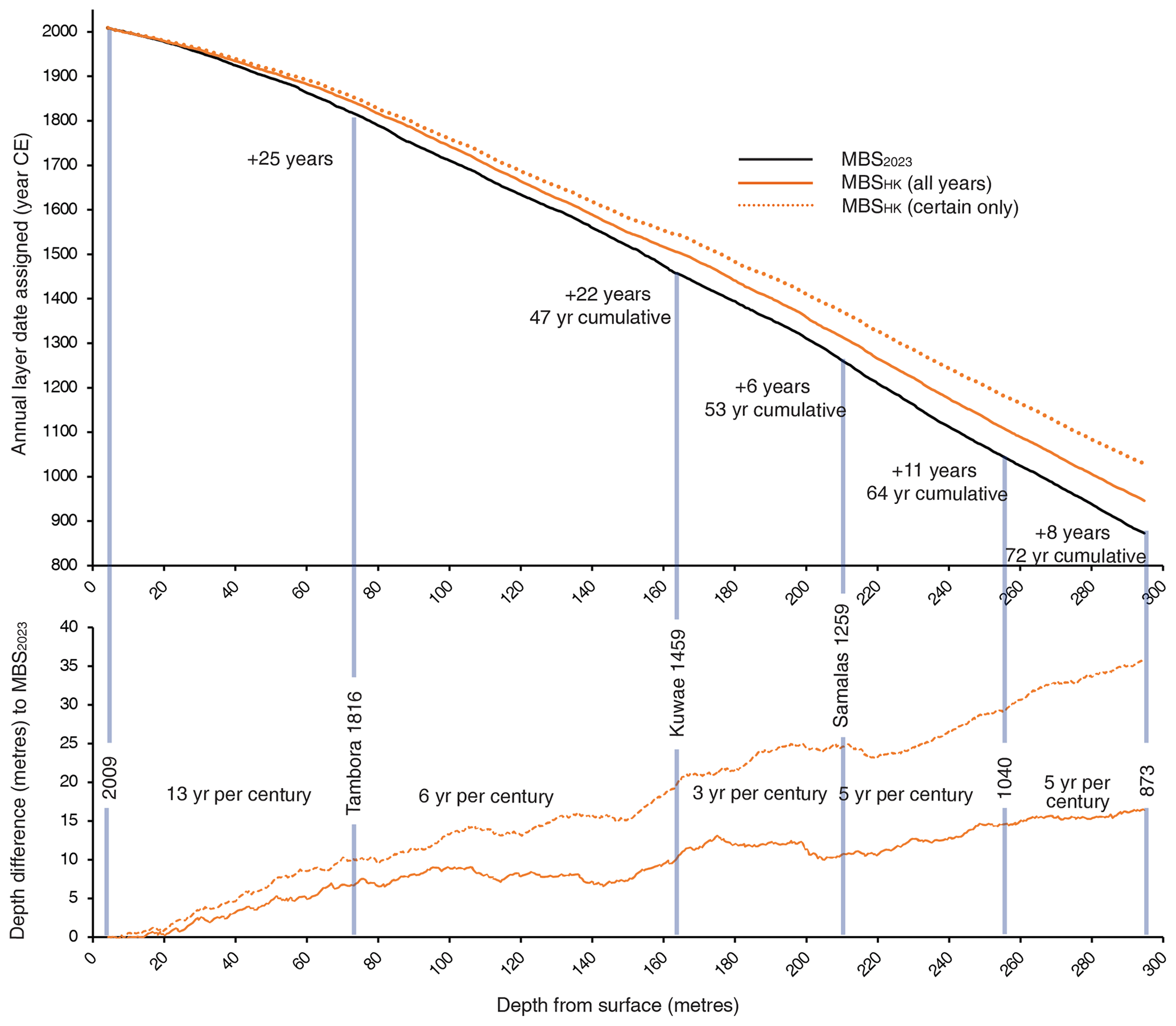
Figure 6Assessing uncertainty from missed annual layers in the MBS ice core records. The upper graph shows the assigned annual layer date by depth between the final Main core chronology (MBS2023, solid black line) compared to layer counting only (MBSHK, solid and dotted orange lines). The layer counting efforts are further distinguished by whether uncertain uncounted annual layers were included or not (solid versus dotted orange lines, respectively). The lower graph illustrates the resultant depth difference in metres for any given assigned annual layer date between the final chronology and the interim age-by-depth scales. Vertical blue lines link assigned annual layer dates at specific volcanic tie points (or the bottom depth at 873 CE or 294.8 m) with their corresponding depth for MBS2023, and link to the depth difference (in metres of ice core) shown in the lower graph. Within each tie point boundary the additional year difference between MBS2023 to MBSHK is indicated, as well as the cumulative difference with increasing depth. For example, from the surface to the 1459 CE Kuwae horizon, there is a depth and age difference of 12.8 m every 47 years, which includes an additional 22 years from the previous tie point at 1816 (Tambora). In the bottom graph, the error rate (in years per century) is indicated for each tie point.
Knowledge that the trace chemistry seasonal cycles deserved at least equal weighting in discerning annual horizons as seasonal variation in the water isotopic ratios became increasingly evident during the group dating process. Ultimately, a cumulative error of 72 uncounted years is accrued in layer counting in MBSHK compared to the synchronized MBS2023, even with uncertain horizons included (Fig. 6). However, we think this error has some mitigating factors. Firstly, the greatest “loss” of annual horizons (25 year) is accrued from the top of the core to the first major tie at Tambora (1816), a rate of 13 years per century. This suggests that this was either a period of “training” for the researcher who produced MBSHK or that the higher number of samples per annual layer in the firn section led to more (rather than less) issues in identifying individual annual horizons. A second reason for the greater error in the upper 200 years is the issues with fluoride analyses in the top 80 m of the MBS Main record (see methods). This meant fluoride was unavailable to assist with dating for this section. After this upper section, the error rate per century drops markedly to 3–6 years per century. We hypothesize that if a new MBS ice core was retrieved and a complete fluoride dataset available, the accumulated knowledge of the inherent idiosyncrasies of the site from this study would result in a much smaller error between a layer-counted-only age-by-depth scale and the final chronology described here.
Curiously, from 1040 CE to the bottom of the core (approximately 40 m), the error rate per century remains similar, despite both efforts comprising layer counting only. We suggest that our four-step dating approach of interim efforts followed by group consensus is thus a robust approach to dating a record with the potential for low and/or episodic accumulation from 1 year to the next as it allows the independent development of age scales that can be compared with a final consensus scale to examine where error is being accrued. In this case, we think that the difference in the age scales from 1040 to the bottom of the core and the lack of a change in the slope of the age scales below 1040 CE indicates development of the dating approach to a new site and the importance of fluoride to the development of the chronology, which has resulted in the robust identification of unclear annual horizons after sequential reviews of the data, even in the absence of volcanic tie points.
4.4 Recommendations arising from this study
We did not make field drawings or take photographs of core orientation, stratigraphic features or drilling damage (e.g. core dog damage) during field processing. Such records would have provided additional physical records of core orientation and features that would have helped solve discrepancies between core lengths measured in the field compared to in the laboratory. In addition, a Japanese pull saw and mitre box or a mechanical drop saw in the field camp would have ensured consistent cuts at 90° to the plane of the core and reduced subsequent errors encountered when constructing the depth model. Nonetheless, the ILCS images of the core we had access to were invaluable in aligning top and bottom depths, and we recommend ILCS image comparisons where possible to ground-truth depth models.
This study provides the individual chronologies (collectively MBS2023) for all MBS cores drilled in 2017/2018 (Main, Alpha, Bravo and Charlie). Given the greater availability of spatial meteorological information since the satellite era in the Southern Hemisphere, users of the MBS ice core records may wish to develop records with as much overlap with the satellite era as possible. In this case, we suggest constructing a composite record using the Main and Charlie (which has a similar range of analyses to the Main core) chronologies to produce a single time series spanning 873–2017 CE. Our suggested compositing point is the annual horizon of 1989/1990 (e.g. the 1 January 1990 horizon). This horizon has a clear and comparatively high peak in δ18O and a correspondingly low and clear summer sea salt minima. It is also prior to the nss signal attributed to the Pinatubo eruption (mid-1991) which can be discerned in all four records (see Fig. 2, Crockart et al., 2021).
Age-by-depth scales and preliminary results from the new Mount Brown South (MBS) ice cores from East Antarctica are presented. We used a four-step approach to develop chronologies for the 295 m “Main” core and three 20–25 m surface cores via layer counting of seasonally varying species and alignment to known volcanic horizons. The MBS “Main” ice core spans 1137±2 years, and the three shallow cores span the recent 4–5 decades up to the surface age at the time of drilling (austral summer 2017/2018). Uncertainty in layer counting is assessed by comparing the final chronology with an interim layer counted only age-by-depth scale to determine the rate of annual horizons missed due to muted seasonal cycles and/or episodic snowfall accumulation. Detection of volcanic horizons is discussed and volcanic sulfate features are compared to other Antarctic ice cores. Mean annual concentrations and seasonal cycles of trace chemistry species are derived and compared to the Law Dome record 1130 km to the east of MBS, with the concentrations of sea salt species and halogens generally less than a quarter of those at Law Dome, probably due to a more continental transport route to the MBS site. Conversely, concentrations of methanesulfonic acid are much higher than at Law Dome, which we attribute to higher local and regional phytoplankton productivity leading to increases in the biogenic precursors of MSA. Finally, we describe a distinct seasonal cycle in fluoride concentrations at MBS that greatly assisted the detection of annual layers and that may contain a climatological signal, which is worthy of future detailed investigation.
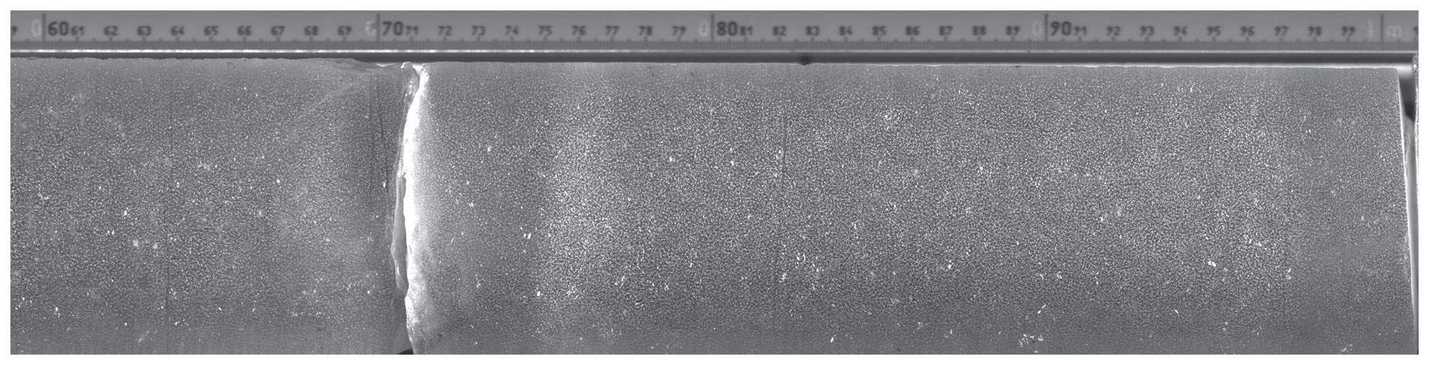
Figure A1An example section of an intermediate-layer ice core scanner (ILCS) image from a deep MBS ice core (core 225, showing a section from 60–100 cm of the core). A slanted cut at the end of the core can be discerned. The ILCS images were used to align and constrain differing core lengths between field and laboratory measurements. A core break (drilling break) can be seen at 71 cm.
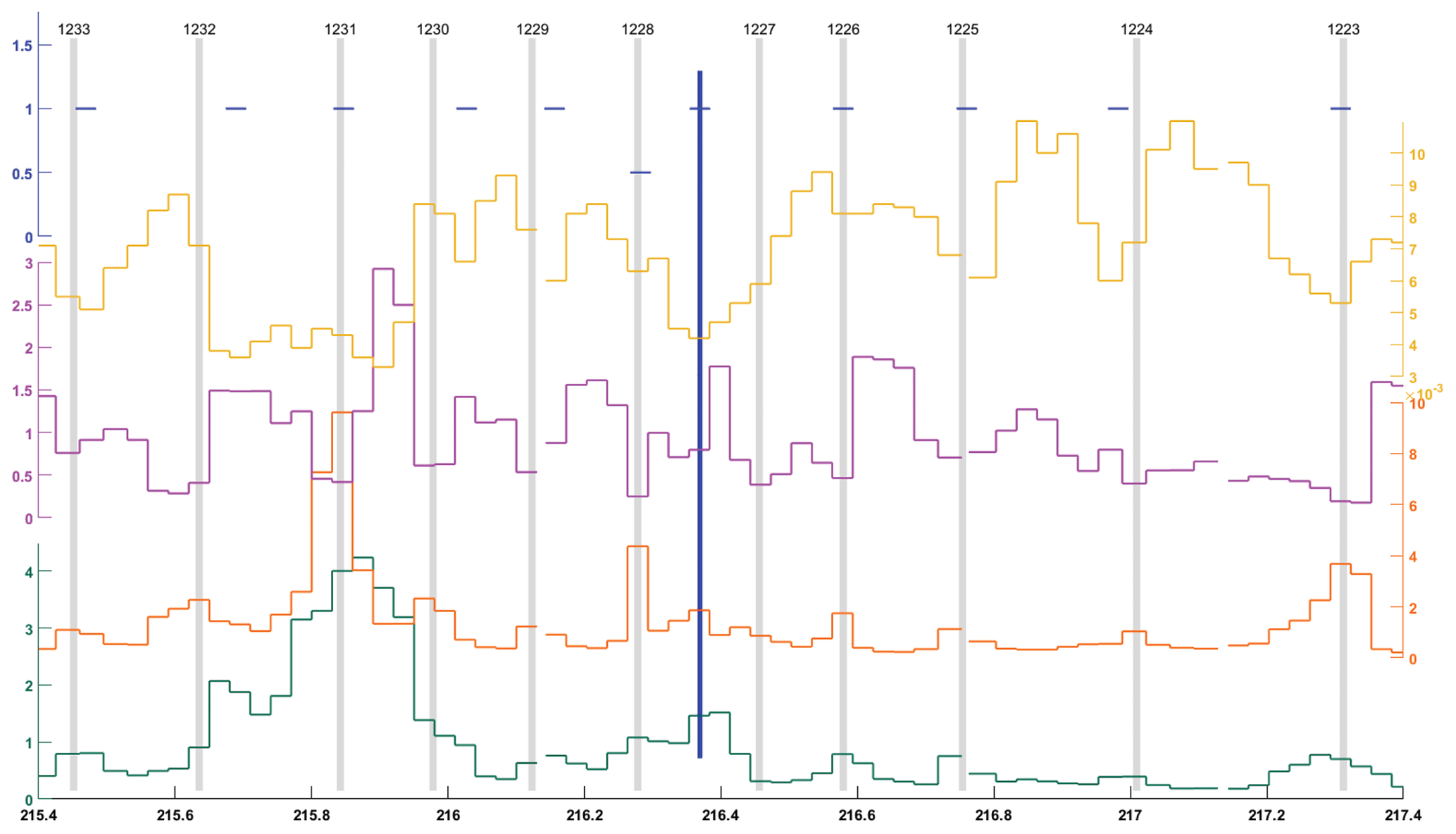
Figure B1An example section of trace chemical data (in µEq L−1) used to identify annual layers in the MBS Main ice core using the Matchmaker program. Ice core depth (m) is on the bottom x axis and the annual horizon placement and year assigned is shown at the top. Trace chemical species used are fluoride (yellow), chloride (pink), sulfate-to-chloride ratio (orange) and non-sea salt sulfate (green). Two different dating efforts are shown – the individual preliminary effort (MBSHK), which has certain years shown as blue horizontal dashes and uncertain years shown as blue dashes at a lower alignment. Vertical lines indicate the final consensus effort of MBS2023, where grey lines represent certain years; bold blue lines represent uncertain counted years (not present in this example); and the thinner, shorter blue line is an example of an uncertain uncounted year. The commencement of a volcanic horizon (unknown) can be seen in the non-sea salt sulfate data at 215.6 m (see Table 3).
The development of MBS2023 followed an initial depth alignment process to develop a final depth scale, followed by individual and group dating efforts. A preliminary step was performed by devising a depth scale incorporating field and laboratory measurements and information from ILCS images. The individual and group dating efforts then followed the steps below.
-
MBSCP-derived layer – an independent interim layer counted age-by-depth scale incorporating alignment to known volcanic horizons.
-
MBSHK-derived layer – an independent interim layer counted only age-by-depth scale incorporating fluoride as a seasonal marker but without alignment to known volcanic horizons.
-
MBSCP- and MBSHK-derived layers were examined together by the dating team, with consensus decisions applied to produce a final age-by-depth scale.
-
FMBS2023 – the final consensus age-by-depth scale after synchronization to WD2014.
Table D1Trace chemistry working standard ranges, representative mean blank values and detection limits for the discrete suppressed ion chromatography analyses performed in Hobart. With the exception of fluoride, detection limits and other analytical parameters are discussed in Curran and Palmer (2001). Detection limits for fluoride were determined in this study according to Armbruster and Pry (2008).
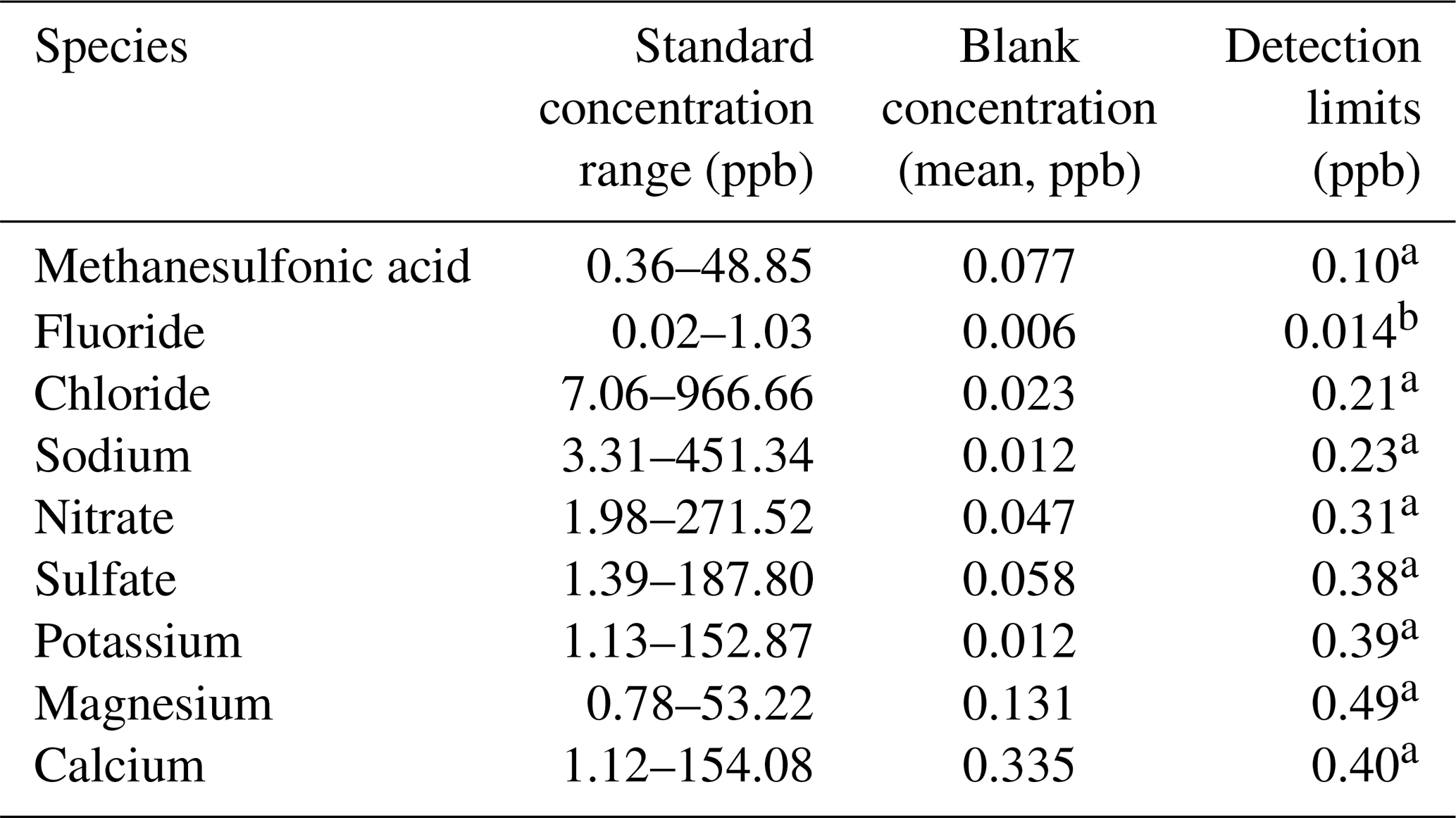
a Curran and Palmer (2001) and b this study.
Annual horizon depths and ages for all Mount Brown South chronologies described here, along with associated data described in this article, are available from the Australian Antarctic Data Centre, https://doi.org/10.26179/352b-6298 (Vance et al., 2024).
TRV designed the study, led the writing with input from all authors, and led the Australian Antarctic Science logistics project to retrieve the ice core. TRV, NJA, ASC, CKC, ADeC, VG, MH, SJ, HAK, CAL, MN, CTP, DS, AS and PTV contributed to drilling, processing, analytical campaigns, production of the depth models, layer counting and data production. VF produced the site climatological data. CTP and HK produced interim age-by-depth scales for comparison.
At least one of the (co-)authors is a member of the editorial board of Climate of the Past. The peer-review process was guided by an independent editor, and the authors also have no other competing interests to declare.
Publisher's note: Copernicus Publications remains neutral with regard to jurisdictional claims made in the text, published maps, institutional affiliations, or any other geographical representation in this paper. While Copernicus Publications makes every effort to include appropriate place names, the final responsibility lies with the authors.
This article is part of the special issue “Ice core science at the three poles (CP/TC inter-journal SI)”. It is a result of the IPICS 3rd Open Science Conference, Crans-Montana, Switzerland, 2–7 October 2022.
We thank Jason Roberts, Sharon Labudda and Bloo Campbell for essential fieldwork contributions and Adam Treverrow for co-designing the ILCS laboratory and planer set-up.
This study was supported by the Australian Government's Antarctic Science Collaboration Initiative (ASCI000002) through funding to the Australian Antarctic Program Partnership. Logistics and analytical funding was provided by an Australian Antarctic Science grant (AAS 4414), the Australian Antarctic Division, the Carlsberg Foundation, and a European Union Horizon 2020 research and innovation grant (TiPES, H2020 grant no. 820970). This study contributes to an Australian Research Council (ARC) Discovery Project (DP220100606) to Tessa R. Vance and Nerilie J. Abram. Nerilie J. Abram was supported by an ARC Future Fellowship (FT160102059), and Nerilie J. Abram and Sarah L. Jackson were supported by the ARC Special Research Initiative Australian Centre of Excellence in Antarctic Science (SR200100008) and the Centre of Excellence for Climate Extremes (CE170100023). Alison S. Criscitiello received support from Polar Knowledge Canada. Vasileios Gkinis acknowledges support from the Villum Foundation (project nos. 00022995, 00028061) and the Danish Independent Research Fund (DFF grant no. 10.46540/2032-00228B). Vincent Favier received support from Agence Nationale de la Recherche, project nos. ANR-20-CE01-0013 (ARCA) and ANR-14-CE01-0001 (ASUMA).
This paper was edited by Alexey Ekaykin and reviewed by Holly Winton and Jacob Chalif.
Abram, N. J., Curran, M. A. J., Mulvaney, R., and Vance, T.: The preservation of methanesulphonic acid in frozen ice-core samples, J. Glaciol., 54, 680–684, https://doi.org/10.3189/002214308786570890, 2008. a
Agosta, C., Amory, C., Kittel, C., Orsi, A., Favier, V., Gallée, H., van den Broeke, M. R., Lenaerts, J. T. M., van Wessem, J. M., van de Berg, W. J., and Fettweis, X.: Estimation of the Antarctic surface mass balance using the regional climate model MAR (1979–2015) and identification of dominant processes, The Cryosphere, 13, 281–296, https://doi.org/10.5194/tc-13-281-2019, 2019. a
Armbruster, D. A. and Pry, T.: Limit of Blank, Limit of Detection and Limit of Quantitation, Clinic. Biochem. Rev., 29, S49–S52, 2008. a
Armstrong, M. S., Kiem, A. S., and Vance, T. R.: Comparing instrumental, palaeoclimate, and projected rainfall data: Implications for water resources management and hydrological modelling, J. Hydrol.: Reg. Stud., 31, 100728, https://doi.org/10.1016/j.ejrh.2020.100728, 2020. a
Bertler, N., Mayewski, P. A., Aristarain, A., et al.: Snow chemistry across Antarctica, Ann. Glaciol., 41, 167–179, https://doi.org/10.3189/172756405781813320, 2005. a
Bigler, M., Svensson, A., Kettner, E., Vallelonga, P., Nielsen, M. E., and Steffensen, J. P.: Optimization of High-Resolution Continuous Flow Analysis for Transient Climate Signals in Ice Cores, Environ. Sci. Technol., 45, 4483–4489, https://doi.org/10.1021/es200118j, 2011. a, b, c, d
Crockart, C. K., Vance, T. R., Fraser, A. D., Abram, N. J., Criscitiello, A. S., Curran, M. A. J., Favier, V., Gallant, A. J. E., Kittel, C., Kjær, H. A., Klekociuk, A. R., Jong, L. M., Moy, A. D., Plummer, C. T., Vallelonga, P. T., Wille, J., and Zhang, L.: El Niño–Southern Oscillation signal in a new East Antarctic ice core, Mount Brown South, Clim. Past, 17, 1795–1818, https://doi.org/10.5194/cp-17-1795-2021, 2021. a, b, c, d, e, f, g, h, i, j, k, l, m, n, o, p, q, r, s, t, u, v
Curran, M. A. and Palmer, A. S.: Suppressed ion chromatography methods for the routine determination of ultra low level anions and cations in ice cores, J. Chromatogr. A, 919, 107–113, https://doi.org/10.1016/s0021-9673(01)00790-7, 2001. a, b
Curran, M. A. J., Ommen, T. D. V., and Morgan, V.: Seasonal characteristics of the major ions in the high-accumulation Dome Summit South ice core, Law Dome, Antarctica, Ann. Glaciol., 27, 385–390, https://doi.org/10.3189/1998AoG27-1-385-390, 1998. a, b
Curran, M. A. J., van Ommen, T. D., Morgan, V. I., Phillips, K. L., and Palmer, A. S.: Ice Core Evidence for Antarctic Sea Ice Decline Since the 1950s, Science, 302, 1203–1206, https://doi.org/10.1126/science.1087888, 2003. a, b
De Angelis, M. and Legrand, M.: Origins and variations of fluoride in Greenland precipitation, J. Geophys. Res.-Atmos., 99, 1157–1172, https://doi.org/10.1029/93JD02660, 1994. a
Eayrs, C., Holland, D., Francis, D., Wagner, T., Kumar, R., and Li, X.: Understanding the Seasonal Cycle of Antarctic Sea Ice Extent in the Context of Longer-Term Variability, Rev. Geophys., 57, 1037–1064, https://doi.org/10.1029/2018RG000631, 2019. a
Erhardt, T., Bigler, M., Federer, U., Gfeller, G., Leuenberger, D., Stowasser, O., Röthlisberger, R., Schüpbach, S., Ruth, U., Twarloh, B., Wegner, A., Goto-Azuma, K., Kuramoto, T., Kjår, H. A., Vallelonga, P. T., Siggaard-Andersen, M.-L., Hansson, M. E., Benton, A. K., Fleet, L. G., Mulvaney, R., Thomas, E. R., Abram, N., Stocker, T. F., and Fischer, H.: High-resolution aerosol concentration data from the Greenland NorthGRIP and NEEM deep ice cores, Earth Syst. Sci. Data, 14, 1215–1231, https://doi.org/10.5194/essd-14-1215-2022, 2022. a
Foster, A. F. M., Curran, M. A. J., Smith, B. T., Ommen, T. D. V., and Morgan, V. I.: Covariation of Sea ice and methanesulphonic acid in Wilhelm II Land, East Antarctica, Ann. Glaciol., 44, 429–432, https://doi.org/10.3189/172756406781811394, 2006. a, b, c
Gkinis, V., Popp, T. J., Johnsen, S. J., and Blunier, T.: A continuous stream flash evaporator for the calibration of an IR cavity ring-down spectrometer for the isotopic analysis of water, Isotop. Environ. Health Stud., 46, 463–475, https://doi.org/10.1080/10256016.2010.538052, 2010. a
Gkinis, V., Popp, T. J., Blunier, T., Bigler, M., Schüpbach, S., Kettner, E., and Johnsen, S. J.: Water isotopic ratios from a continuously melted ice core sample, Atmos. Meas. Tech., 4, 2531–2542, https://doi.org/10.5194/amt-4-2531-2011, 2011. a
Gorodetskaya, I. V., Tsukernik, M., Claes, K., Ralph, M. F., Neff, W. D., and Van Lipzig, N. P. M.: The role of atmospheric rivers in anomalous snow accumulation in East Antarctica, Geophys. Res. Lett., 41, 6199–6206, https://doi.org/10.1002/2014GL060881, 2014. a
Jackson, S. L., Vance, T. R., Crockart, C., Moy, A., Plummer, C., and Abram, N. J.: Climatology of the Mount Brown South ice core site in East Antarctica: implications for the interpretation of a water isotope record, Clima. Past, 19, 1653–1675, https://doi.org/10.5194/cp-19-1653-2023, 2023. a, b, c, d, e, f, g, h, i, j, k, l, m, n, o
Johnsen, S. J., Hansen, S. B., Sheldon, S. G., Dahl-Jensen, D., Steffensen, J. P., Augustin, L., Journé, P., Alemany, O., Rufli, H., Schwander, J., Azuma, N., Motoyama, H., Popp, T., Talalay, P., Thorsteinsson, T., Wilhelms, F., and Zagorodnov, V.: The Hans Tausen drill: design, performance, further developments and some lessons learned, Ann. Glaciol., 47, 89–98, https://doi.org/10.3189/172756407786857686, 2007. a
Jones, J. M., Gille, S. T., Goosse, H., Abram, N. J., Canziani, P. O., Charman, D. J., Clem, K. R., Crosta, X., de Lavergne, C., Eisenman, I., England, M. H., Fogt, R. L., Frankcombe, L. M., Marshall, G. J., Masson-Delmotte, V., Morrison, A. K., Orsi, A. J., Raphael, M. N., Renwick, J. A., Schneider, D. P., Simpkins, G. R., Steig, E. J., Stenni, B., Swingedouw, D., and Vance, T. R.: Assessing recent trends in high-latitude Southern Hemisphere surface climate, Nat. Clim. Change, 6, 917–926, https://doi.org/10.1038/nclimate3103, 2016. a, b
Jong, L. M., Plummer, C. T., Roberts, J. L., Moy, A. D., Curran, M. A. J., Vance, T. R., Pedro, J. B., Long, C. A., Nation, M., Mayewski, P. A., and van Ommen, T. D.: 2000 years of annual ice core data from Law Dome, East Antarctica, Earth Syst. Sci. Data, 14, 3313–3328, https://doi.org/10.5194/essd-14-3313-2022, 2022. a, b, c, d, e, f, g, h, i, j
Kaufmann, P. R., Federer, U., Hutterli, M. A., Bigler, M., Schüpbach, S., Ruth, U., Schmitt, J., and Stocker, T. F.: An Improved Continuous Flow Analysis System for High-Resolution Field Measurements on Ice Cores, Environ. Sci. Technol., 42, 8044–8050, https://doi.org/10.1021/es8007722, 2008. a
Kiem, A. S., Vance, T. R., Tozer, C. R., Roberts, J. L., Pozza, R. D., Vitkovsky, J., Smolders, K., and Curran, M. A. J.: Learning from the past – Using palaeoclimate data to better understand and manage drought in South East Queensland (SEQ), Australia, J. Hydrol.: Reg. Stud., 29, 100686, https://doi.org/10.1016/j.ejrh.2020.100686, 2020. a
Kjær, H. A., Vallelonga, P., Svensson, A., Elleskov, L., Kristensen, M., Tibuleac, C., Winstrup, M., and Kipfstuhl, S.: An Optical Dye Method for Continuous Determination of Acidity in Ice Cores, Environ. Sci. Technol., 50, 10485–10493, https://doi.org/10.1021/acs.est.6b00026, 2016. a
Kjær, H. A., Zens, P., Black, S., Lund, K. H., Svensson, A., and Vallelonga, P.: Canadian forest fires, Icelandic volcanoes and increased local dust observed in six shallow Greenland firn cores, Clim. Past, 18, 2211–2230, https://doi.org/10.5194/cp-18-2211-2022, 2022. a, b, c
Legrand, M., Léopold, A., and Dominé, F.: Acidic Gases (HCl, HF, HN03, HCOOH, and CH3COOH): A Review of Ice Core Data and Some Preliminary Discussions on their Air-Snow Relationships, in: Chemical Exchange Between the Atmosphere and Polar Snow, edited by Wolff, E. W. and Bales, R. C., NATO ASI Series, Springer, Berlin, Heidelberg, 19–43, ISBN 978-3-642-61171-1, https://doi.org/10.1007/978-3-642-61171-1_2, 1996. a
McGwire, K. C., McConnell, J. R., Alley, R. B., Banta, J. R., Hargreaves, G. M., and Taylor, K. C.: Dating annual layers of a shallow Antarctic ice core with an optical scanner, J. Glaciol., 54, 831–838, https://doi.org/10.3189/002214308787780021, 2008. a, b
Morganti, A., Becagli, S., Castellano, E., Severi, M., Traversi, R., and Udisti, R.: An improved flow analysis–ion chromatography method for determination of cationic and anionic species at trace levels in Antarctic ice cores, Anal. Chim. Acta, 603, 190–198, https://doi.org/10.1016/j.aca.2007.09.050, 2007. a
Orsi, A. J., Kawamura, K., Fegyveresi, J. M., Headly, M. A., Alley, R. B., and Severinghaus, J. P.: Differentiating bubble-free layers from melt layers in ice cores using noble gases, J. Glaciol., 61, 585–594, https://doi.org/10.3189/2015JoG14J237, 2015. a
Palmer, A. S., Morgan, V. I., Curran, M. A. J., Ommen, T. D. v., and Mayewski, P. A.: Antarctic volcanic flux ratios from Law Dome ice cores, Ann. Glaciol., 35, 329–332, https://doi.org/10.3189/172756402781816771, 2002. a
Plummer, C. T., Curran, M. A. J., van Ommen, T. D., Rasmussen, S. O., Moy, A. D., Vance, T. R., Clausen, H. B., Vinther, B. M., and Mayewski, P. A.: An independently dated 2000-yr volcanic record from Law Dome, East Antarctica, including a new perspective on the dating of the 1450s CE eruption of Kuwae, Vanuatu, Clim. Past, 8, 1929–1940, https://doi.org/10.5194/cp-8-1929-2012, 2012. a, b, c, d, e, f, g, h, i, j
Pohl, B., Favier, V., Wille, J., Udy, D. G., Vance, T. R., Pergaud, J., Dutrievoz, N., Blanchet, J., Kittel, C., Amory, C., Krinner, G., and Codron, F.: Relationship Between Weather Regimes and Atmospheric Rivers in East Antarctica, J. Geophys. Res.-Atmos., 126, e2021JD035294, https://doi.org/10.1029/2021JD035294, 2021. a
Preunkert, S., Legrand, M., and Wagenbach, D.: Causes of enhanced fluoride levels in Alpine ice cores over the last 75 years: Implications for the atmospheric fluoride budget, J. Geophys. Res.-Atmos., 106, 12619–12632, https://doi.org/10.1029/2000JD900755, 2001. a
Raphael, M. N. and Handcock, M. S.: A new record minimum for Antarctic sea ice, Nat. Rev. Earth Environ., 3, 215–216, https://doi.org/10.1038/s43017-022-00281-0, 2022. a
Roach, L. A., Eisenman, I., Wagner, T. J. W., Blanchard-Wrigglesworth, E., and Bitz, C. M.: Asymmetry in the seasonal cycle of Antarctic sea ice driven by insolation, Nat. Geosci., 15, 277–281, https://doi.org/10.1038/s41561-022-00913-6, 2022. a
Roberts, J., Plummer, C., Vance, T., van Ommen, T., Moy, A., Poynter, S., Treverrow, A., Curran, M., and George, S.: A 2000-year annual record of snow accumulation rates for Law Dome, East Antarctica, Clim. Past, 11, 697–707, https://doi.org/10.5194/cp-11-697-2015, 2015. a, b
Roberts, J. L., Ommen, T. D. V., Curran, M. A. J., and Vance, T. R.: Methanesulphonic acid loss during ice-core storage: recommendations based on a new diffusion coefficient, J. Glaciol., 55, 784–788, https://doi.org/10.3189/002214309790152474,2009. a
Robinson, J., Popova, E. E., Srokosz, M. A., and Yool, A.: A tale of three islands: Downstream natural iron fertilization in the Southern Ocean, J. Geophys. Res.-Oceans, 121, 3350–3371, https://doi.org/10.1002/2015JC011319, 2016. a
Sanz Rodriguez, E., Plummer, C., Nation, M., Moy, A., Curran, M., Haddad, P. R., and Paull, B.: Sub-1 mL sample requirement for simultaneous determination of 17 organic and inorganic anions and cations in Antarctic ice core samples by dual capillary ion chromatography, Anal. Chim. Acta, 1063, 167–177, https://doi.org/10.1016/j.aca.2019.02.014, 2019. a, b, c, d
Schallenberg, C., Bestley, S., Klocker, A., Trull, T. W., Davies, D. M., Gault‐Ringold, M., Eriksen, R., Roden, N. P., Sander, S. G., Sumner, M., Townsend, A. T., Merwe, P., Westwood, K., Wuttig, K., and Bowie, A.: Sustained Upwelling of Subsurface Iron Supplies Seasonally Persistent Phytoplankton Blooms Around the Southern Kerguelen Plateau, Southern Ocean, J. Geophys. Res.-Oceans, 123, 5986–6003, https://doi.org/10.1029/2018JC013932, 2018. a
Schüpbach, S., Fischer, H., Bigler, M., Erhardt, T., Gfeller, G., Leuenberger, D., Mini, O., Mulvaney, R., Abram, N. J., Fleet, L., Frey, M. M., Thomas, E., Svensson, A., Dahl-Jensen, D., Kettner, E., Kjaer, H., Seierstad, I., Steffensen, J. P., Rasmussen, S. O., Vallelonga, P., Winstrup, M., Wegner, A., Twarloh, B., Wolff, K., Schmidt, K., Goto-Azuma, K., Kuramoto, T., Hirabayashi, M., Uetake, J., Zheng, J., Bourgeois, J., Fisher, D., Zhiheng, D., Xiao, C., Legrand, M., Spolaor, A., Gabrieli, J., Barbante, C., Kang, J.-H., Hur, S. D., Hong, S. B., Hwang, H. J., Hong, S., Hansson, M., Iizuka, Y., Oyabu, I., Muscheler, R., Adolphi, F., Maselli, O., McConnell, J., and Wolff, E. W.: Greenland records of aerosol source and atmospheric lifetime changes from the Eemian to the Holocene, Nat. Commun., 9, 1476, https://doi.org/10.1038/s41467-018-03924-3,2018. a, b
Severi, M., Becagli, S., Frosini, D., Marconi, M., Traversi, R., and Udisti, R.: A Novel Fast Ion Chromatographic Method for the Analysis of Fluoride in Antarctic Snow and Ice, Environ. Sci. Technol., 48, 1795–1802, https://doi.org/10.1021/es404126z, 2014. a
Sheldon, S. G., Popp, T. J., Hansen, S. B., Hedegaard, T. M., and Mortensen, C.: A new intermediate-depth ice-core drilling system, Ann. Glaciol., 55, 271–284, https://doi.org/10.3189/2014AoG68A038, 2014a. a
Sheldon, S. G., Popp, T. J., Hansen, S. B., and Steffensen, J. P.: Promising new borehole liquids for ice-core drilling on the East Antarctic high plateau, Ann. Glaciol., 55, 260–270, https://doi.org/10.3189/2014AoG68A043, 2014b. a
Sigl, M., Fudge, T. J., Winstrup, M., Cole-Dai, J., Ferris, D., McConnell, J. R., Taylor, K. C., Welten, K. C., Woodruff, T. E., Adolphi, F., Bisiaux, M., Brook, E. J., Buizert, C., Caffee, M. W., Dunbar, N. W., Edwards, R., Geng, L., Iverson, N., Koffman, B., Layman, L., Maselli, O. J., McGwire, K., Muscheler, R., Nishiizumi, K., Pasteris, D. R., Rhodes, R. H., and Sowers, T. A.: The WAIS Divide deep ice core WD2014 chronology – Part 2: Annual-layer counting (0–31 ka BP), Clim. Past, 12, 769–786, https://doi.org/10.5194/cp-12-769-2016, 2016. a, b, c
Smith, B. T., Ommen, T. D. V., and Morgan, V. I.: Distribution of oxygen isotope ratios and snow accumulation rates in Wilhelm II Land, East Antarctica, Ann. Glaciol., 35, 107–110, https://doi.org/10.3189/172756402781816898, 2002. a, b
Stenni, B., Curran, M. A. J., Abram, N. J., Orsi, A., Goursaud, S., Masson-Delmotte, V., Neukom, R., Goosse, H., Divine, D., van Ommen, T., Steig, E. J., Dixon, D. A., Thomas, E. R., Bertler, N. A. N., Isaksson, E., Ekaykin, A., Werner, M., and Frezzotti, M.: Antarctic climate variability on regional and continental scales over the last 2000 years, Clim. Past, 13, 1609–1634, https://doi.org/10.5194/cp-13-1609-2017, 2017. a
Svensson, A., Nielsen, S. W., Kipfstuhl, S., Johnsen, S. J., Steffensen, J. P., Bigler, M., Ruth, U., and Röthlisberger, R.: Visual stratigraphy of the North Greenland Ice Core Project (NorthGRIP) ice core during the last glacial period, J. Geophys. Res.-Atmos., 110, D02108, https://doi.org/10.1029/2004JD005134, 2005. a
Talalay, P., Hu, Z., Xu, H., Yu, D., Han, L., Han, J., and Wang, L.: Environmental considerations of low-temperature drilling fluids, Ann. Glaciol., 55, 31–40, https://doi.org/10.3189/2014AoG65A226, 2014. a
Thomas, E. R., van Wessem, J. M., Roberts, J., Isaksson, E., Schlosser, E., Fudge, T. J., Vallelonga, P., Medley, B., Lenaerts, J., Bertler, N., van den Broeke, M. R., Dixon, D. A., Frezzotti, M., Stenni, B., Curran, M., and Ekaykin, A. A.: Regional Antarctic snow accumulation over the past 1000 years, Clim. Past, 13, 1491–1513, https://doi.org/10.5194/cp-13-1491-2017, 2017. a
Thomas, E. R., Vladimirova, D. O., Tetzner, D. R., Emanuelsson, B. D., Chellman, N., Dixon, D. A., Goosse, H., Grieman, M. M., King, A. C. F., Sigl, M., Udy, D. G., Vance, T. R., Winski, D. A., Winton, V. H. L., Bertler, N. A. N., Hori, A., Laluraj, C. M., McConnell, J. R., Motizuki, Y., Takahashi, K., Motoyama, H., Nakai, Y., Schwanck, F., Simões, J. C., Lindau, F. G. L., Severi, M., Traversi, R., Wauthy, S., Xiao, C., Yang, J., Mosely-Thompson, E., Khodzher, T. V., Golobokova, L. P., and Ekaykin, A. A.: Ice core chemistry database: an Antarctic compilation of sodium and sulfate records spanning the past 2000 years, Earth Syst. Sci. Data, 15, 2517–2532, https://doi.org/10.5194/essd-15-2517-2023, 2023. a
Trevena, A. J. and Jones, G. B.: Dimethylsulphide and dimethylsulphoniopropionate in Antarctic sea ice and their release during sea ice melting, Mar. Chem., 98, 210–222, https://doi.org/10.1016/j.marchem.2005.09.005, 2006. a, b
Trevena, A. J., Jones, G. B., Wright, S. W., and van den Enden, R. L.: Profiles of DMSP, algal pigments, nutrients and salinity in pack ice from eastern Antarctica, J. Sea Res., 43, 265–273, https://doi.org/10.1016/S1385-1101(00)00012-5, 2000. a
Trevena, A. J., Jones, G. B., Wright, S. W., and van den Enden, R. L.: Profiles of dimethylsulphoniopropionate (DMSP), algal pigments, nutrients, and salinity in the fast ice of Prydz Bay, Antarctica, J. Geophys. Res.-Oceans, 108, 3145, https://doi.org/10.1029/2002JC001369, 2003. a
Turner, J., Phillips, T., Thamban, M., Rahaman, W., Marshall, G. J., Wille, J. D., Favier, V., Winton, V. H. L., Thomas, E., Wang, Z., van den Broeke, M., Hosking, J. S., and Lachlan-Cope, T.: The Dominant Role of Extreme Precipitation Events in Antarctic Snowfall Variability, Geophys. Res. Lett., 46, 3502–3511, https://doi.org/10.1029/2018GL081517, 2019. a, b
Udy, D. G., Vance, T. R., Kiem, A. S., Holbrook, N. J., and Curran, M. A. J.: Links between Large-Scale Modes of Climate Variability and Synoptic Weather Patterns in the Southern Indian Ocean, J. Climate, 34, 883–899, https://doi.org/10.1175/JCLI-D-20-0297.1, 2021. a, b
Udy, D. G., Vance, T. R., Kiem, A. S., and Holbrook, N. J.: A synoptic bridge linking sea salt aerosol concentrations in East Antarctic snowfall to Australian rainfall, Commun. Earth Environ., 3, 1–11, https://doi.org/10.1038/s43247-022-00502-w, 2022. a, b, c
Vallelonga, P., Maffezzoli, N., Moy, A. D., Curran, M. A. J., Vance, T. R., Edwards, R., Hughes, G., Barker, E., Spreen, G., Saiz-Lopez, A., Corella, J. P., Cuevas, C. A., and Spolaor, A.: Sea-ice-related halogen enrichment at Law Dome, coastal East Antarctica, Clim. Past, 13, 171–184, https://doi.org/10.5194/cp-13-171-2017, 2017. a, b, c, d
Vallelonga, P., Maffezzoli, N., Saiz-Lopez, A., Scoto, F., Kjær, H. A., and Spolaor, A.: Sea-ice reconstructions from bromine and iodine in ice cores, Quaternary Sci. Rev., 269, 107133, https://doi.org/10.1016/j.quascirev.2021.107133, 2021. a
Vance, T. R., Davidson, A. T., Thomson, P. G., Levasseur, M., Lizotte, M., Curran, M. A. J., and Jones, G. B.: Rapid DMSP production by an Antarctic phytoplankton community exposed to natural surface irradiances in late spring, Aquat. Microb. Ecol., 71, 117–129, https://doi.org/10.3354/ame01670, 2013. a
Vance, T. R., Roberts, J. L., Moy, A. D., Curran, M. A. J., Tozer, C. R., Gallant, A. J. E., Abram, N. J., van Ommen, T. D., Young, D. A., Grima, C., Blankenship, D. D., and Siegert, M. J.: Optimal site selection for a high-resolution ice core record in East Antarctica, Clim. Past, 12, 595–610, https://doi.org/10.5194/cp-12-595-2016, 2016. a, b, c
Vance, T. R., Kiem, A. S., Jong, L. M., Roberts, J. L., Plummer, C. T., Moy, A. D., Curran, M. A. J., and van Ommen, T. D.: Pacific decadal variability over the last 2000 years and implications for climatic risk, Commun. Earth Environ., 3, 1–9, https://doi.org/10.1038/s43247-022-00359-z, 2022. a, b
Vance, T. R., Abram, N. J., Gkinis, V., Harlan, M., Jackson, S., Plummer, C., Segato, D., Spolaor, A., and Vallelonga, P.: MBS2023 – The Mount Brown South Main ice core chronology and chemistry data and surface core chronologies, Ver. 1, Australian Antarctic Data Centre [data set], https://doi.org/10.26179/352b-6298, 2024. a
van Ommen, T. D. and Morgan, V.: Calibrating the ice core paleothermometer using seasonality, J. Geophys. Res.-Atmos., 102, 9351–9357, https://doi.org/10.1029/96JD04014, 1997. a, b, c, d
Westhoff, J., Sinnl, G., Svensson, A., Freitag, J., Kjær, H. A., Vallelonga, P., Vinther, B., Kipfstuhl, S., Dahl-Jensen, D., and Weikusat, I.: Melt in the Greenland EastGRIP ice core reveals Holocene warm events, Clima. Past, 18, 1011–1034, https://doi.org/10.5194/cp-18-1011-2022, 2022. a
Wille, J. D., Favier, V., Gorodetskaya, I. V., Agosta, C., Kittel, C., Beeman, J. C., Jourdain, N. C., Lenaerts, J. T. M., and Codron, F.: Antarctic Atmospheric River Climatology and Precipitation Impacts, J. Geophys. Res.-Atmos., 126, e2020JD033788, https://doi.org/10.1029/2020JD033788, 2021. a
Winstrup, M., Svensson, A. M., Rasmussen, S. O., Winther, O., Steig, E. J., and Axelrod, A. E.: An automated approach for annual layer counting in ice cores, Clim. Past, 8, 1881–1895, https://doi.org/10.5194/cp-8-1881-2012, 2012. a
Winstrup, M., Vallelonga, P., Kjær, H. A., Fudge, T. J., Lee, J. E., Riis, M. H., Edwards, R., Bertler, N. A. N., Blunier, T., Brook, E. J., Buizert, C., Ciobanu, G., Conway, H., Dahl-Jensen, D., Ellis, A., Emanuelsson, B. D., Hindmarsh, R. C. A., Keller, E. D., Kurbatov, A. V., Mayewski, P. A., Neff, P. D., Pyne, R. L., Simonsen, M. F., Svensson, A., Tuohy, A., Waddington, E. D., and Wheatley, S.: A 2700-year annual timescale and accumulation history for an ice core from Roosevelt Island, West Antarctica, Clim. Past, 15, 751–779, https://doi.org/10.5194/cp-15-751-2019, 2019. a, b, c, d
Zhang, L., Vance, T. R., Fraser, A. D., Jong, L. M., Thompson, S. S., Criscitiello, A. S., and Abram, N. J.: Identifying atmospheric processes favouring the formation of bubble-free layers in the Law Dome ice core, East Antarctica, The Cryosphere, 17, 5155–5173, https://doi.org/10.5194/tc-17-5155-2023, 2023. a, b
- Abstract
- Introduction
- Methods
- Results
- Discussion
- Conclusions
- Appendix A: Example ILCS image
- Appendix B: Annual layer counting example
- Appendix C: Dating procedure summary
- Appendix D: Ion chromatography standard ranges, detection limits and representative blank values
- Data availability
- Author contributions
- Competing interests
- Disclaimer
- Special issue statement
- Acknowledgements
- Financial support
- Review statement
- References