A continental reconstruction of hydroclimatic variability in South America during the past 2000 years

Paleoclimatological field reconstructions are valuable for understanding past hydroclimatic variability, which is crucial for assessing potential future hydroclimate changes. Despite being as impactful on societies as temperature variability, hydroclimatic variability – particularly beyond the instrumental record – has received less attention. The reconstruction of globally complete fields of climate variables lacks adequate proxy data from tropical regions like South America, limiting our understanding of past hydroclimatic changes in these areas. This study addresses this gap using low-resolution climate archives, including speleothems, previously omitted from reconstructions. Speleothems record climate variations on decadal to centennial timescales and provide a rich dataset for the otherwise proxy-data-scarce region of tropical South America. By employing a multi-timescale paleoclimate data assimilation approach, we synthesize climate proxy records and climate model simulations capable of simulating water isotopologs in the atmosphere to reconstruct 2000 years of South American climate. This includes surface air temperature, precipitation amount, drought index, isotopic composition of precipitation amount and the intensity of the South American Summer Monsoon. The reconstruction reveals anomalous climate periods: a wetter and colder phase during the Little Ice Age (∼ 1500–1850 CE) and a drier, warmer period corresponding to the early Medieval Climate Anomaly (∼ 600–900 CE). However, these patterns are not uniform across the continent, with climate trends in northeastern Brazil and the Southern Cone not following the patterns of the rest of the continent, indicating regional variability. The anomalies are more pronounced than in previous reconstructions but match trends found in local proxy record studies, thus highlighting the importance of including speleothem proxies. The multi-timescale approach is essential for reconstructing multi-decadal and centennial climate variability. Despite methodological uncertainties regarding climate model biases and proxy record interpretations, this study marks a crucial first step in incorporating low-resolution proxy records such as speleothems into climate field reconstructions using a multi-timescale approach. Adequately extracting and using the information from speleothems potentially enhances insights into past hydroclimatic variability and hydroclimate projections.

1 Introduction

The climate of the Common Era (CE), which spans the last 2 millennia, is considered the most thoroughly studied preindustrial paleoclimatic period owing to the abundance of records from various paleoclimate archives (PAGES 2k Consortium, 2019) and climate observations. It provides rather stable, close-to-present-day boundary conditions prior to the onset of industrialization, with a relatively constant greenhouse gas concentration and sea level and climate variability due to natural, solar and volcanic forcings. Thus, it represents a well-studied benchmark for climate models (e.g., Jungclaus et al., 2017). Over the last 2 millennia, the global climate has presented itself as an interplay and superposition of various major atmospheric and oceanic modes of variability. As such, different regions of South America are influenced by the El Niño–Southern Oscillation (ENSO), the Pacific Decadal Oscillation (PDO), the Atlantic Multidecadal Oscillation (AMO), the Southern Annular Mode (SAM) and variations in the position of the Intertropical Convergence Zone (ITCZ) (Garreaud et al., 2009). The spatial and temporal variability of the South American Summer Monsoon (SASM) (Zhou and Lau, 1998; Marengo et al., 2010) and its subcomponent, the South Atlantic Convergence Zone (SACZ) (Carvalho et al., 2004), creates a wide range of climate zones across the continent. This makes the South American continent an intriguing test bed for climatological research into the interplay of different phenomena before the onset of the current warming period.

The challenges posed by anthropogenic climate change are particularly pronounced in South America. The implications for water resources are significant, given that South America comprises two of the world's most crucial river basins: the Amazon Basin in the center and north of the continent and the Paraná–La Plata Basin in the center and southeast of the continent. However, the broader effects of anthropogenic climate change on the entire hydrological cycle and its variability, including changes in precipitation extremes and the occurrence of droughts, remain less studied than for temperature. Improving the understanding of the full range of climate variability in South America is imperative, given the high vulnerability of human livelihoods in tropical and subtropical regions to the impacts of climate change. This vulnerability is especially evident in extreme events like droughts and floods due to both geographic and socioeconomic factors (IPCC, 2022), as seen for example in the current megadrought in central Chile (Garreaud et al., 2019).

The climate of the past beyond the instrumental period is studied to enhance our understanding of hydroclimate and contextualize recent changes.

For instance, extreme events and their socioeconomic consequences have been recorded in historical documents (Prieto and García Herrera, 2009), such as a sequence of droughts in northeastern Brazil (Aceituno et al., 2008; Utida et al., 2023), droughts in Bolivia (Gioda and Prieto, 1999) and extreme floods of the Paraná River (Prieto, 2007).

Climate archives are increasingly used to reconstruct and interpret changes in climate beyond the instrumental era. These reconstructions offer statistically robust estimates of the climate, particularly for the CE, the period of interest in our study. In principle, existing global climate field reconstructions of the CE already provide estimates for both surface temperature and hydroclimate variables, including for South America (e.g., Hakim et al., 2016; Franke et al., 2017; Steiger et al., 2018; Tardif et al., 2019; Neukom et al., 2019). However, global CE reconstructions predominantly rely on proxy records from the mid-to-high latitudes, particularly tree rings from the Northern Hemisphere. The climate proxy record density for the CE in tropical and subtropical regions is much lower, in particular for terrestrial locations (Neukom and Gergis, 2012). Terrestrial proxy records are, however, crucial when it comes to reconstructing hydroclimatic variability. Although climate field reconstruction can make use of teleconnections to alleviate data scarcity, the lack of local data limits the viability of global reconstruction in (sub)tropical regions (Anchukaitis and Smerdon, 2022).

For South America, climate field reconstructions are constrained by the scarcity of climate proxy records for all regions except for the central and southern Andes, where tree rings serve as an abundant climate archive. Regional climate field reconstructions have thus primarily focused on southern South America (Neukom et al., 2010, 2011; Boucher et al., 2011; Luterbacher et al., 2011; Morales et al., 2020). However, in recent years, speleothems have emerged as a promising climate archive with the potential to alleviate data scarcity in tropical South America (Vuille et al., 2012). Speleothems are geological cave formations created by accumulating layers of calcium carbonates transported by seepage water. Among the many climate proxies archived in speleothems, the ratio between heavy and light oxygen isotopes (δ¹⁸O) saved in accumulating layers of calcium carbonate reflects the isotopic composition of the precipitation above a cave and, thus, records hydroclimatic changes (Bradley, 2015). The δ¹⁸O signatures of precipitation are sensitive to air temperature; precipitation amount changes; and the geographical location in terms of altitude, latitude and distance from the coast (Dansgaard, 1964).

For South America, particularly in the region influenced by the South American Summer Monsoon (SASM), the primary driver of δ¹⁸O signatures in precipitation is the amount of rainfall during the monsoon season rather than the temperature (Vuille et al., 2003; Moquet et al., 2016). Additionally, the δ¹⁸O signatures are influenced by the location of the moisture source, notably the moisture contribution from the ITCZ region, and the degree of upstream rainout, which captures the precipitation history of the air mass along its trajectory, as demonstrated by cave-monitoring studies (Ampuero et al., 2020; Jiménez-Iñiguez et al., 2022; Moquet et al., 2016) and modeling studies (Vuille et al., 2003; Vuille and Werner, 2005; Vuille et al., 2012) that work with station data from the Global Network of Isotopes in Precipitation (GNIP) (IAEA/WMO, 2020). δ¹⁸O in speleothems in tropical South America is thus closely linked to changes in both regional and large-scale atmospheric circulation patterns.

Tropical South America is an archetypical region for speleothem research, with a growing number of published records in recent years. For instance, single records have been used to demonstrate changes in the intensity of the SASM on millennial to centennial timescales in response to changes in orbital and solar forcing (Novello et al., 2016; Bernal et al., 2016). For the hydroclimate of the last millennium, pronounced anomalies found in speleothem δ¹⁸O values have been associated with the Medieval Climate Anomaly (MCA) and the Little Ice Age (LIA) (Novello et al., 2018; Apaéstegui et al., 2018; Azevedo et al., 2019). Moreover, through the analysis of several South American speleothem records using dimensionality-reduction techniques, Orrison et al. (2022) demonstrated that climate model simulations of the last millennium consistently underestimate centennial climate changes over the South American continent, reinforcing findings by Rojas et al. (2016), who investigated SASM variability in climate model simulations.

It is not clear if existing climate field reconstructions include these insights into South American hydroclimate variability during the CE due to the limited integration of speleothem records. Their incorporation proves difficult for two main reasons. First, reconstructions of the CE are usually attempted at seasonal or annual resolution and, thus, only include proxy records of at least annual resolution. Speleothems are seldom dated annually; dating uncertainties are often on the order of several years. Even so, karst processes above the caves work as smoothing filters for the isotopic variations in precipitation. Thus, speleothem δ¹⁸O time series reflect the mixing of rainfall from different seasons and the transit time through the epikarst to the water dripping point in the cave (for speleothems in Brazil, see Moquet et al., 2016). Second, climate field reconstructions usually require a calibration of the proxy records to instrumental data. This calibration is hampered by the low temporal resolution of speleothem records and the short data overlap with regional instrumental observations. Similar restrictions also apply to many lake and marine sediments, precluding their use in current climate field reconstructions. In this study, we aim to overcome these limitations to explore the information gain associated with including previously excluded climate archives of annual to decadal resolution.

Here, we present the first climate field reconstruction of the hydroclimate of the South American continent for the entire CE, which is achieved by employing speleothems besides more commonly used climate archives such as tree rings, lake sediments, ice cores, corals, sclerosponges, marine sediments and historical documents. We combine proxy records from a multitude of proxy record databases (Emile-Geay et al., 2017; Comas-Bru et al., 2020; Konecky et al., 2020; Morales et al., 2020; Neukom et al., 2009) and individual records provided by original authors. This yields a total of 307 proxy records (see Fig. 1). Our selection currently represents the most spatially complete collection of publicly available proxy record data for the region.

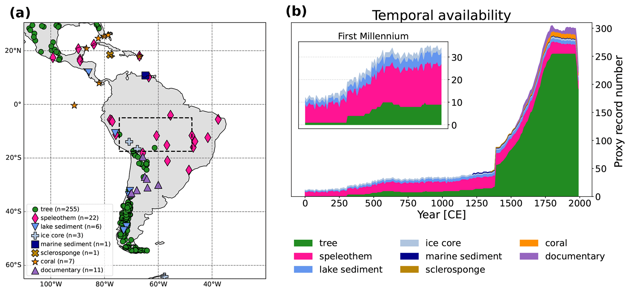
Figure 1 Spatiotemporal availability of the employed proxy records. (a) Spatial distribution of all employed proxy records. Archive types are encoded by shape and color. The represented spatial domain (65° S–35° N, 20–110° W) is the spatial domain reconstructed in this study. In addition, the black box demarcates the core region of the South American Summer Monsoon (SASM) following the definition by Vuille et al. (2012), which we use to reconstruct the SASM index. (b) Temporal availability of proxy archive types, with a zoom of the first millennium.

We choose to use paleoclimate data assimilation (PaleoDA) (Bhend et al., 2012; Steiger et al., 2014) as the climate field reconstruction technique. Based on the principles of DA, which has been successfully applied in weather and ocean forecasting for 3 decades (Evensen et al., 2022), PaleoDA fuses information from climate model simulations and climate observations to provide a best state estimate. In contrast to other regression-based techniques (e.g., principal-component regression, as in Luterbacher et al., 2002; Neukom et al., 2014), PaleoDA does not directly rely on gridded instrumental datasets. The climate simulations provide time series that are long enough to also include proxy records of relatively low resolution, such as speleothems, which cannot be calibrated to instrumental data. We use five state-of-the-art isotope-enabled climate simulations which simulate the isotopic composition of precipitation and which were made publicly available recently (Bühler et al., 2022b). Employing these previously unused simulations in PaleoDA provides a twofold information gain: first, it enables the inclusion of speleothem records in the PaleoDA without the uncertainties associated with instrumental calibration, and second, it facilitates the comparison of multiple simulations of rainfall δ¹⁸O values from different models, thereby mitigating biases stemming from individual proxies and models. In this study, we will focus on surface temperature, precipitation amount, SPEI (standardized precipitation evapotranspiration index, a drought index; Vicente-Serrano et al., 2010; Beguería et al., 2014), and the isotopic composition of precipitation. While, in theory, PaleoDA allows climate fields to be reconstructed for all simulated climate variables, the chosen variables are most closely related to the climate signal recorded by the selected climate archives and, thus, hold the highest potential for reliable reconstructions. To overcome the difficulties posed by proxy records of annual to decadal resolution such as speleothems, we adapt the PaleoDA algorithm to a multi-timescale method, enhancing the concept proposed by Steiger and Hakim (2016).

The structure of this study is as follows. We introduce the proxy record and climate model simulation data on which we base our reconstruction. We then provide a complete description of the multi-timescale PaleoDA methodology, its assumptions and key parameters. We present our obtained reconstruction (for both annual and austral-summer means) and validate it by means of comparison to instrumental data, other reconstructions and non-assimilated proxy record data. As one of several climatological applications of the reconstruction dataset, we study the main centennial hydroclimatological changes in South America during the MCA and the LIA and assess if our reconstruction aligns with insights from other studies. In addition, we investigate the reconstructed intensity and variability of the SASM using a precipitation-based monsoon index, which has not been studied in climate field reconstructions before.

2 Data

2.1 Paleoclimate proxy data

The continental climate field reconstruction provided in this study is based on a selection of different climate archive types. While focusing on climate archives that store information about the hydroclimate, we also include other types of archives to better cover the range of variables. The archives include trees, speleothems, ice cores, lake sediments, corals, sclerosponges and marine sediments. To ensure the best possible spatiotemporal coverage of the region, we have chosen and combined proxy records from three published paleoclimate proxy databases: PAGES2k (Emile-Geay et al., 2017); Iso2k (Konecky et al., 2020); the third version of the database from the Speleothem Isotopes Synthesis and AnaLysis working group, SISALv3 (Atsawawaranunt et al., 2018; Comas-Bru et al., 2020; Kaushal et al., 2024); tree rings used for the South American Drought Atlas (Morales et al., 2020); and historical documentary indices presented by Neukom et al. (2009). We additionally included single proxy records which are currently not included in published proxy record databases (see the individual references in Sect. S1.2 in the Supplement). In contrast to the other proxy record databases, the SISALv3 speleothem database has not been employed in climate field reconstruction previously.

The SISALv3 database provides different sets of chronologies for the different speleothems. For this analysis, we use the authors' original chronology only. Further, age uncertainties, which are only provided for SISALv3, are not explicitly considered, as these are mostly smaller than the time steps in the multi-timescale PaleoDA algorithm (see Sect. 3.2). A description table for each climate archive type that we included, including metadata for the individual proxy records, the proxy variable, the median resolution and methodological choices (proxy system model, assumed noise, seasonality and timescale), is provided in Tables S1.1 to S1.7.

We define four selection criteria for choosing proxy records from the respective databases:

1. The sites where the climate archives were obtained are located in the region 65° S–35° N, 20–110° W (see Fig. 1). Proxy records from Central America are explicitly included as they can provide information for the northern part of South America, for which there are few proxy records for the past 2 millennia.

2. The proxy variable is approximately linearly related to one of the climate variables provided by the climate model simulations (see Sects. 2.2 and 3.3). We follow the recommendations given by the authors in the original publications to decide if such a relationship holds. Note, that speleothem and ice core δ¹⁸O values can also be included in our proxy record collection because the climate model data also includes the simulated isotopic composition of rainfall.

3. The proxy records span at least 200 years and have at least one sample value in the period from 1750 to 1850 CE. This period is used as the reference period for computing anomalies of the proxy records relative to a shared time period. It has the advantage of including crucial records, such as speleothems, that lack data points during the more commonly chosen reference period of the 20th century. At the same time, this excludes many shorter records which would lead to high reconstruction skill during the instrumental era but would not contribute to the reconstruction of centennial-scale hydroclimate changes and are, thus, acceptable to omit.

4. The resolution of the proxy records is better than 10 years (median), as we set the largest reconstruction timescale in the multi-timescale paleodata assimilation approach (described in Sect. 3.2) to 10 years. While decadal to multi-decadal or lower resolution is technically possible, the proxy records that fall into that category are too coarsely resolved to contribute to the skill of the reconstruction of the past 2 millennia on multi-decadal and centennial timescales, which is the focus of this study.

Our selection of proxy records for the South American reconstruction consists of 307 records covering South and Central America (Fig. 1). Due to our selection criteria, the number of available proxy records was highest for the reference period 1750–1850 CE and lowest for the first century (13 records). Despite the decreasing number of available proxy records earlier during the CE, the spatial coverage remains fairly similar throughout time, as the older proxy records are evenly distributed. This is particularly evident for tree rings, which are clustered in the Andes (see also Fig. S1.1 for the spatiotemporal availability of proxy records for each reconstructed century). The temporal availability of proxy records shows a sharp decline in tree ring data in the year 1400 CE, coinciding with the start of the SADA tree ring database. Throughout the reconstruction, we remain attentive to potential artifacts resulting from this decline. Despite this concern, we anticipate only a small impact, given that the tree rings are situated in regions where there are already proxy records. Non-speleothem archives mostly cover the central and southern Andes and coastal regions, while speleothems significantly contribute to the coverage of tropical inner-continental regions over the entire 2 millennia. Regions lacking archive sites for proxy records can be found in the northern part of South America, namely Colombia, the Guianas and the northwestern states of Brazil. Additionally, the western part of the Southern Cone, the cone-shaped area of South America south of the Tropic of Capricorn (∼ 23.4° S), lacks proxy records. However, the South American Drought Atlas has demonstrated that tree ring records from the central and southern Andes can be skillfully used to reconstruct the hydroclimate of that region. The northern part of the Southern Cone is covered by documentary data from the 16th century on.

2.2 Isotope-enabled climate model simulations

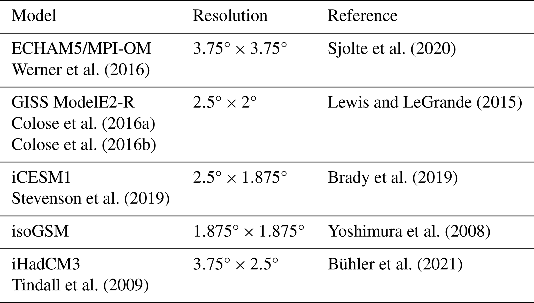
We use five state-of-the-art isotope-enabled climate model simulations of the last millennium (Bühler et al., 2022a and Table 1). Additional information about boundary conditions and forcing parameters can be found in Bühler et al. (2022a). Isotope-enabled climate models are essential for our study as they allow us to bypass the uncertain calibration of speleothem δ¹⁸O records against temperature or precipitation. From the simulations, we use the following variables: surface temperature, total precipitation amount and isotopic precipitation. SPEI (standardized precipitation evapotranspiration index, a drought index; Vicente-Serrano et al., 2010) is computed from simulated precipitation and temperature using the code based on Thornthwaite's method for estimating potential evapotranspiration from the climate-indices package (Adams, 2017). The timescale is set to 12 months. We choose Thornthwaite's method over the more precise Penman–Monteith formula because the available climate model simulation data do not include all the variables required for the latter. In parts of the analysis, we use a multi-model ensemble (MME) by conducting separate reconstructions for each model prior and then computing the mean of the five reconstructions. In PaleoDA, MMEs are used to provide more reliable reconstructions than provided by single-model priors (Parsons et al., 2021; Annan et al., 2022; King et al., 2021, 2023). As we will use the climate model data only as anomalies, the purpose of the MME in this study is not to alleviate the effect of mean-value biases in the models but to provide a more diverse covariance structure, which constitutes the backbone of the PaleoDA reconstruction algorithm (see Sect. 3.1). This covariance structure across models is particularly relevant in our study, as the covariance relationships between δ¹⁸O and other climate variables such as temperature and precipitation vary considerably in the different climate models. An MME requires the regridding of all climate model simulations to the same grid. We choose to interpolate all climate model simulations to the highest resolution provided by one of our input models, isoGSM (1.875° × 1.875°). This allows the spatial information of the higher-resolution models to be kept. Computing the correlation fields for the regridded climate fields, we found that the regridding produces smoothed correlation fields without introducing artifacts (not shown). Note that it is also conceivable to construct an MME by concatenating the model priors before applying the ensemble Kalman filter equations, but this method is not used here.

Sjolte et al. (2020)Werner et al. (2016)Lewis and LeGrande (2015)Colose et al. (2016a)Colose et al. (2016b)Brady et al. (2019)Stevenson et al. (2019)Yoshimura et al. (2008)Bühler et al. (2021)Tindall et al. (2009)

Table 1 Spatial resolutions of and references for the isotope-enabled last-millennium simulations used in this study. The references listed in the Reference column also include the model descriptions. For a detailed description of the boundary conditions and forcing parameters, see Bühler et al. (2022a).

3 Methods

3.1 Data assimilation with the ensemble Kalman filter as a climate field reconstruction technique

Data assimilation (DA), which has been developed mainly for improving numerical weather and ocean fore- and hindcasts, combines two sets of information: (i) a statistical prior state estimate that is provided by an ensemble of estimates from a numerical model and (ii) information from observations (e.g., climate proxy records). The prior estimate is updated conditional on the observations (Evensen et al., 2022). The obtained posterior state is then propagated through time by the numerical model until new observations are available. PaleoDA often simplifies some aspects of DA compared to operational weather- and ocean-forecasting systems, particularly by omitting the model ensemble restart step due to the limited predictability and the computational cost of general circulation models (GCMs) on paleoclimatic timescales (Dirren and Hakim, 2005; Huntley and Hakim, 2010). Figure S2.1 illustrates the main steps of the PaleoDA algorithm. Here, the updating operation is performed by the ensemble Kalman filter (EnKF) (Evensen, 1994), which assumes that the prior and the observations are sampled from the same true but unknown Gaussian distribution. The errors with respect to the true distribution are assumed to be unbiased and normally distributed. The EnKF further assumes that the observations are linearly related to the true distribution. Despite the normality assumptions, it has proven to be also a good estimator in nonlinear cases where the assumptions do not strictly hold, which explains its wide use in real-world applications (Evensen et al., 2022). In the last decade, the EnKF has been introduced into the field of climate field reconstructions (Bhend et al., 2012; Steiger et al., 2014) and has been used to reconstruct the climate of the last 2 millennia (e.g., Hakim et al., 2016; Steiger et al., 2018; Tardif et al., 2019) and older periods such as the Last Glacial Maximum (Tierney et al., 2020; Annan et al., 2022), the last deglaciation (Osman et al., 2021; Erb et al., 2022) and the Paleocene–Eocene Thermal Maximum (Tierney et al., 2022).

The EnKF assimilation equation states that

$$\begin{array}{}\text{(1)}& \mathbf{X}=\widehat{\mathbf{X}}+\mathbf{K}(\mathbf{Y}-\mathcal{H}\widehat{\mathbf{X}}),\end{array}$$

where $\widehat{\mathbf{X}}$ is the prior state (e.g., the surface temperature field over all simulated time steps, which creates an ensemble) and X is the posterior state matrix. Y is the observation vector containing the proxy record values at a specific time step, and ℋ is the observation operator mapping the prior values to the observations (further explained in Sect. 3.3), thus creating $\mathcal{H}\widehat{\mathbf{X}}$, the observation estimates for the simulated values. K is the Kalman gain matrix, a weighting matrix, which blends the prior state estimate and observations according to covariances in the prior ensemble and the proxy record uncertainty. It is computed as

$$\begin{array}{}\text{(2)}& \mathbf{K}=\text{cov}(\mathbf{X},\mathcal{H}(\mathbf{X}\left)\right)\left(\text{cov}\right(\mathcal{H}\left(\mathbf{X}\right),\mathcal{H}\left(\mathbf{X}\right))+\mathbf{R}{)}^{-\mathrm{1}}.\end{array}$$

R is the observation error covariance matrix, which contains the error associated with the proxy records (see Sect. 3.4). We assume that the observation errors of different proxy records are uncorrelated; hence, R is a diagonal matrix. The EnKF assimilation equation can be effectively described as an interpolation process where the model prior provides covariance estimates between observation locations and all simulated locations, which are used to perform the interpolation. Equation (2) follows upon minimizing the posterior error covariance matrix, which is given by

$$\begin{array}{}\text{(3)}& \text{cov}(\mathbf{X},\mathbf{X})=(\mathbf{I}-\mathbf{K}\mathcal{H})\text{cov}(\widehat{\mathbf{X}},\widehat{\mathbf{X}}).\end{array}$$

The uncertainty of the reconstructed variables at each time step can be computed as the standard deviations of the diagonal entries of the posterior error covariance matrix (Eq. 3). The posterior covariance matrix is, by construction, less than or equal to the prior covariance. To solve Eqs. (1), (2) and (3) efficiently, we utilize the ensemble transform Kalman filter (Bishop et al., 2001), as formulated in Vetra-Carvalho et al. (2018). Instead of restarting the model ensemble, the prior covariance matrix $\widehat{\mathbf{X}}$ from already-computed simulations is used and thus represents the climatological covariance. To compute it, we use an ensemble of 100 randomly selected simulation years (see Sect. 3.5). This approach has been named stationary offline PaleoDA (Okazaki et al., 2021) and assumes stationary covariance between climate variables at the grid cells. Each year is reconstructed separately, with the temporal pacing determined by the climate proxy records and the spatial information provided by the covariances from the climate model simulations. Note that by using an MME (Sect. 2.2), we effectively use the mean Kalman gain from the five model priors. The offline PaleoDA concept is similar to computationally efficient optimal/statistical interpolation methods (Evensen, 2003; Oke et al., 2005), although they still forward a single-model simulation in time according to the results of the assimilation.

We reconstruct both annual (April–March, according to the vegetation cycle) and austral-summer (DJF) means separately because the selected proxy records likely represent either annual or summer means (in particular speleothems from the SASM region).

In our reconstruction, the prior ensemble mean for each grid cell and climate variable is always forced to be zero to limit model mean-value biases. We consider this a valid approach as the CE is a relatively stable climatic period. Not performing such debiasing would introduce steplike, unphysical shifts in the reconstructed time series, depending on the availability of a specific proxy record with a strong difference from the prior (as also noted in Franke et al. (2017), for example).

3.2 Multi-timescale paleoclimate data assimilation

The PaleoDA algorithm described in Sect. 3.1 is usually employed for the assimilation of proxy records at a single timescale, e.g., annual or seasonal for the CE. However, the speleothem records that are the backbone of our regional reconstruction have median temporal resolutions of 1 to 8 years and actually represent smoothed climate signals due to mixing effects of the karst system on the cave drip water (Moquet et al., 2016). Therefore, we developed a new multi-timescale adaptation of the EnKF–PaleoDA algorithm, building on the concept proposed by Steiger and Hakim (2016), which allows us to use low- and high-resolution proxy records simultaneously in a computationally efficient manner.

The key idea is to add an additional time dimension for consecutive years to the prior state matrix X, enabling the use of multi-year means and covariances in the PaleoDA algorithm (see Fig. S2.2). The number of years added to the prior state matrix is determined by the largest timescale imposed by the proxy records, which we determine to be the decadal timescale for the employed speleothems. Instead of reconstructing the target time period (1–2000 CE) year by year, we divide it into decadal blocks, as we will use the speleothem values on a decadal timescale only. Additionally, we reconstruct annual and quinquennial timescales as sub-blocks of the decadal block (see Fig. S2.3). The decadal prior block is the same during the entire reconstruction period. For each decadal block, the algorithm computes the assimilation equations for all proxy records that represent the largest timescale, using decadal means in the prior state matrix. The resulting decadal mean value is then exchanged in the prior state matrix. The algorithm continues with the smaller timescales using the corresponding proxy records. Each proxy record is used on a single timescale. This procedure requires resampling the records to the target resolution of the desired timescale prior to the data assimilation. We first bin all the non-annual proxy records to the respective resolution using a simple equidistancing resampling routine, which consists of upsampling the time series values to annual resolution, filtering the time series with a low-pass filter and finally resampling to the targeted resolution (similar to the MakeEquidistant function of the Paleospec R package; Laepple et al., 2023a). We ensure that the resampling does not add spurious data points by choosing target resolutions that are larger than the largest proxy record sampling interval, and we mask longer gaps in the proxy records. The multi-timescale algorithm involves more calculation steps than the single-timescale algorithm due to the repeated calculation of multi-year means and anomalies in the prior state matrix. As such, the algorithm also requires the repeated application of the observation operator ℋ in the Kalman filter equations. However, this is avoided by appending the observation estimates to the prior state matrix such that the algorithm also updates the observation estimates. A multi-timescale paleoclimate data assimilation approach is not only advantageous because it allows for the assimilation of irregular proxy records; it should also improve the reconstruction of multi-decadal to centennial climate variability according to pseudoproxy experiments (Steiger and Hakim, 2016; Choblet et al., 2023). Note that this multi-timescale PaleoDA algorithm differs from the one used in the Holocene temperature reconstruction by Erb et al. (2022), where the multi-timescale prior ensemble is constructed as a moving prior ensemble from transient climate simulations.

3.3 Proxy system models

In PaleoDA, proxy system models (PSMs) (Evans et al., 2013; Dee et al., 2015) are employed for the observation operator ℋ in Eqs. (1) and (2). These were developed to enhance the model–data comparison by encapsulating the physical, geological, biological and biogeochemical processes into mathematical formulas to translate the external climatic conditions into a proxy record signal. These processes are usually divided into three different stages: the sensor, archive and observation stages. In this study, we use PSMs in a one-stage manner, which is common in PaleoDA studies targeting the CE climate (e.g., Hakim et al., 2016; Steiger et al., 2018; Tardif et al., 2019). Within this PaleoDA study, the PSMs translate the signal of the simulated climate to proxy record units (the proxy record variance), accounting for seasonality. We employ three types of PSMs, depending on the nature of the proxy records:

• a.

  For records already calibrated to temperature, such as some lake and marine sediments and sclerosponges, the PSM takes the temperature of the model grid box closest to the proxy record location as the simulated temperature value. Seasonal means or annual means (April to March) are used, depending on the indications in the original publication of the record. In this way, seasonal biases in the reconstruction are constrained.

• b.

  For proxy records that reflect changes in δ¹⁸O of precipitation, such as speleothems, ice cores and some lake sediments, the PSM uses the simulated δ¹⁸O of precipitation values from the closest locations to the proxy records. Annual means of the precipitation-weighted δ¹⁸O values are computed to account for varying precipitation intensity over the year. The values of the two ice core records given in deuterium are divided by 8 to represent the variability in δ¹⁸O according to the Global Meteoric Water Line (Craig, 1961). Although the δ¹⁸O values in these different archives are stored in different materials (e.g., ice, carbonates and trees) and, thus, have different mean values, this is not relevant for our reconstruction because we use proxy record anomalies with respect to a reference period. We assume that temperature-dependent fractionation effects are small compared to the variation in the δ¹⁸O of precipitation values.

• c.

  For proxy records that can be calibrated to instrumental data, such as corals, tree rings and documentary indices, we employ a linear-regression-based PSM, as usually employed in PaleoDA (e.g., Hakim et al., 2016; Steiger et al., 2018; Tardif et al., 2019; King et al., 2021; Sanchez et al., 2021; Valler et al., 2024). While more specific PSMs for corals and tree rings exist, linear-regression-based PSMs yield similar reconstruction results in PaleoDA (Dee et al., 2016). More complex PSMs for corals and tree rings also require environmental variables for sea water and air moisture, which are not available for all of the employed climate model simulations. Furthermore, we consider it preferable to use this type of univariate linear PSM in PaleoDA, as the covariance relationship between observations and the reconstructed climate field remains more tractable. Linear regression equations between the proxy time series and instrumental time series over a calibration period are estimated. The regression parameters are then applied to the model data in the data assimilation. Different predictor variables such as surface temperature, precipitation or SPEI (a drought index) are used, based on the lowest p value for each proxy record. For coral records, we only use surface temperature as a predictor variable. We use the Berkeley Earth dataset for surface temperature (Rohde and Hausfather, 2020), precipitation from CRUTS 4 (Harris et al., 2020b) and the SPEI computed from the temperature and precipitation in CRUTS 4 as instrumental calibration datasets. The temperature calibration is performed over the period 1920–2000 CE. For precipitation and SPEI, we use the period 1950–2000 CE due to the limited local station data in South America before 1950 CE (Garreaud et al., 2009). These spatially highly resolved instrumental datasets have been regridded to the spatial resolution used in the climate field reconstruction to account for the lower spatial resolution of the climate model simulation data. We compute these regressions for both the annual and the seasonal instrumental means and choose the best predictor variable separately (as in Steiger et al., 2018). For the annual reconstruction, 110 tree-ring records were predicted with the temperature, 94 were predicted with the SPEI and 51 were predicted with the precipitation. One historical documentary record was predicted with the temperature, four were predicted with the SPEI and nine were predicted with the precipitation. For the austral-summer reconstruction, 102 tree-ring records were predicted with the temperature, 92 were predicted with the SPEI and 61 were predicted with the precipitation, whereas two historical documentary records were predicted with the temperature, six were predicted with the SPEI and three were predicted with the precipitation.

3.4 The proxy record error

The proxy record error in data assimilation represents the non-climatic noise recorded by proxy records and is challenging to quantify. Measurement noise is considered negligible. For the tree, coral and documentary archives, where calibration could be performed with instrumental data, the proxy error follows directly from the linear regression in the PSM (see Sect. 3.3). The mean of the squared linear-regression residuals is the proxy error variance. For all other records in the non-instrumental era, we express the proxy record error in terms of the signal-to-noise ratio (SNR), assuming Gaussian and timescale-independent noise (Smerdon, 2012). We assume an SNR of 0.5 for all proxy records which we have not calibrated to instrumental variables, following exploratory studies by Wang et al. (2014) and Orrison et al. (2022). The SNR can then be converted into the entries in the observation error matrix R in Eq. (2) by taking into account the variance of the proxy records, var(Y) (see Sect. S2.2 for the derivation):

$$\begin{array}{}\text{(4)}& {\displaystyle }\mathbf{R}=\text{var}\left(\mathbf{Y}\right)/(\mathrm{1}+{\text{SNR}}^{\mathrm{2}}).\end{array}$$

R is computed for each proxy record that cannot be calibrated using its resampled time series (see Sect. 3.2). Given that some proxy records, particularly speleothems, exhibit significant shifts in local climate or environment, we observed that the variance and thus R would be larger compared to those that do not show such local changes. Consequently, the former records exerted less influence during the reconstruction. To address this issue, we used the mean of the variance in a running 200-year window for computing var(Y) to reduce the influence of shifts on the variance and to ensure that noise levels are comparable for all proxy records. We thus assume that for a 200-year window, the statistical assumptions of Gaussian and timescale-independent noise that lead to Eq. (4) hold. We emphasize that the proxy record error should not be considered separately from the variance in the prior ensemble matrix, which represents the model error (see Eq. 1). The relationship between proxy error and prior variance is crucial in PaleoDA. While the static prior variance is usually considered to be too large and is thus reduced by a factor (e.g., Oke et al., 2005) in regular data assimilation via the optimal interpolation method, climate simulations have been allegedly underestimating climate variability – for instance in surface temperature (Laepple and Huybers, 2014; Laepple et al., 2023b) or isotopic variability in precipitation (Bühler et al., 2022a) – which could be used as an argument in favor of inflating the variance in the prior. Instead of adjusting the variance in the prior, we also performed alternative reconstructions in which the proxy error variance for non-calibratable records was set equal to the variance in the prior observation estimates. This approach gives equal weight to the proxy observations and the model prior.

3.5 Further reconstruction refinements

We use a Monte Carlo technique, repeating the reconstructions 50 times with different ensembles of 100 randomly selected simulation years and using 80 % of all proxy records in each repetition, similar to Hakim et al. (2016) and Tardif et al. (2019). Doing so improves the representation of the reconstruction uncertainty and attenuates the effect of outliers in the proxy record selection and the prior ensemble provided by the climate model simulations, as suggested by pseudoproxy experiments. The withheld proxy records are used for the internal validation of the reconstruction. Covariance localization, which is used to suppress spurious long-range covariances, is not employed in this study because the prior ensemble size is considered large. Furthermore, PaleoDA studies that use covariance localization usually do so with very large decorrelation lengths – larger than 12 000 km (e.g., Tardif et al., 2019; Tierney et al., 2020; Osman et al., 2021), exceeding the targeted area in our reconstruction.

4 Validation

We validate our reconstruction using gridded instrumental data sets from the 20th century, independent reconstructions and proxy records withheld from the reconstruction. The focus here is placed on the internal validation using withheld proxy records, as performed in previous PaleoDA studies (e.g., Tardif et al., 2019; King et al., 2021; Tierney et al., 2020; Osman et al., 2021). The reason for doing so is that, although instrumental validations are commonly used in PaleoDA and most are easy to interpret, we do not consider them representative in our case due to the shortness of the instrumental record compared to our decadal and quinquennial climate archives. The instrumental temperature and precipitation time series are too short to validate a decadal-scale reconstruction. The 20th-century validation mainly reflects the reconstruction capability of tree rings, which are the most abundant climate archive in the instrumental period but only provide limited spatial and temporal coverage during the entire CE. The inclusion of speleothems in this study mainly relies on the assumption that their δ¹⁸O signatures capture the monsoon variability, which is locally validated in Moquet et al. (2016) and Jiménez-Iñiguez et al. (2022). Correlation analysis of the model data supports the validity of this assumption in our reconstruction. An extensive validation using gridded instrumental temperature and precipitation data for evaluating the reconstruction regionally and for the SASM precipitation amount is presented in Sects. S3.1 and S3.2. A validation of the reconstructed drought index for the Southern Cone, for which independent reconstructions exist, is presented in Sect. S3.3.

Withholding proxy records in each repetition of the repeated Monte Carlo reconstructions allows us to perform an internal validation of the reconstruction (see Sect. 3.5). The proxy record estimates from the simulation data (e.g., the simulated isotopic composition of precipitation in the grid cell in which a cave is located) remain part of the prior state matrix when a proxy is not used as input data and is therefore updated in the PaleoDA algorithm. We calculate the correlation and coefficient of efficiency (COE) (Nash and Sutcliffe, 1970) of the withheld proxy record time series with respect to their reconstructed counterparts. While the correlation rewards the correct timings of the reconstructed values, the COE is also sensitive to bias and errors in the amplitude as it takes into account the variance of the true signal. The COE can take values in the range [$-\mathrm{\infty },\mathrm{1}$], with positive values indicating skill. However, as pointed out by Cook et al. (1999) and Hakim et al. (2016), the coefficient of efficiency (COE) can misleadingly yield negative skill scores when the proxy records and reconstructions have different mean values, and thus the comparison to the prior can be more meaningful than the raw skill scores. We therefore also compute these scores for the prior model simulations and compare the obtained values to those of our reconstruction. To enable a fair comparison between model priors and reconstructions, the skill scores are computed for the period 850–1850 CE, which is the period covered by the model simulations. The correlation and COE are computed as the mean correlation for all Monte Carlo repetitions in which a proxy record is not used by resampling the reconstructed time series to the respective temporal resolution of each proxy record. As we performed 50 Monte Carlo reconstructions with 20 % of the proxy records withheld, there are on average 10 reconstructions in which a particular proxy record has not been used as input data. This allows us to assess if the reconstruction is in accordance with independent proxy record data and to indirectly identify regions in which proxy data share a common climate signal and are similarly reconstructed. The results are displayed in the form of histograms and on maps in Fig. 2. We obtain predominantly positive correlations (73.29 %), with a median value of 0.17. Almost half of the correlations are positive and significant (45.60 %). As the correlations of the model simulations to the proxy records are negligible, the reconstruction does lead to a clear improvement in correlation, with a median increase of 0.16 and with 71.99 % of the records showing an improvement. However, a few records stand out due to negative correlations in the reconstruction, particularly in geographically isolated areas, while higher correlations are generally obtained in regions with numerous proxy records. For the COE, the obtained median value is −0.01. Yet, 42.02 % of the values result in a positive COE. In comparison to the model priors, there is a notable median increase of 0.37, with 90.23 % of the records demonstrating an improved COE value and thus skill of the reconstruction.

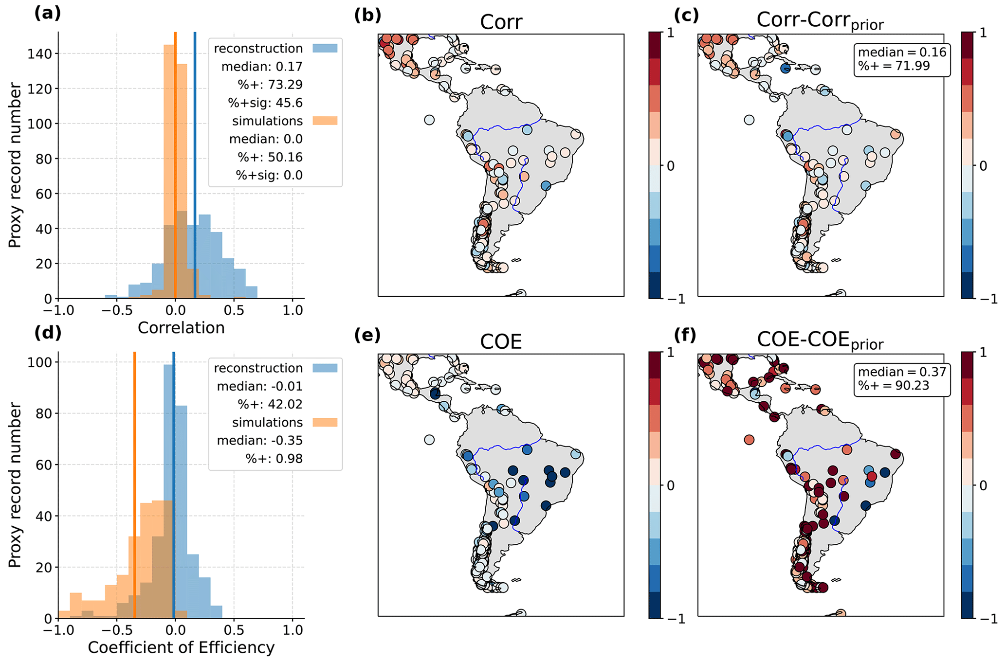
Figure 2 We compute the correlation (a, b, c) and coefficient of efficiency (COE) (d, e, f) of the reconstructed proxy record time series with respect to the true proxy record time series when the proxy records are not used as input data in the reconstruction (withheld proxy records). Panels (a) and (d) show histograms of the skill scores. The box in the upper right corner displays the median value, the percentage of positive values (%+) and the percentage of positive and significant correlations (%+sig, p value <0.05) for the distributions. Panels (b) and (e) display the skill scores for each location. We additionally computed the skill scores for the model simulations (the mean of the five models for each proxy record), which are also included in the histograms and used for a comparison between the reconstruction skill scores and the model simulations (c, f). Note that the COE can also take values smaller than −1. In effect, 25 % of the COE values for the simulations fall outside of the histogram. While all color bars have been limited to the range ($-\mathrm{1},\mathrm{1}$) for clarity, values in (e) and (f) can be more negative than −1, and the difference between the reconstruction and simulations in (f) can also be larger than 1.

The COE score results underscore the high dissimilarity of proxy records for northern and eastern Brazil, which is possibly linked to the climate dipole between northeastern Brazil and the core SASM region (Novello et al., 2018; Campos et al., 2019; Wong et al., 2021), for which speleothem records exhibit opposing δ¹⁸O trends. This spatial homogeneity in the reconstruction may potentially mask this crucial feature of the South American climate. Such homogeneity is expected due to the coarse model grid resolution and the spatial smoothing of the EnKF-based reconstruction method, in contrast to the high spatial variability of the proxy records. While the raw skill values appear low, they are comparable to those obtained in a global multi-proxy reconstruction by Hakim et al. (2016); Tardif et al. (2019); King et al. (2021). The comparison to the skill scores of the prior model simulations emphasizes that the assimilated product represents the climate signal of the proxy records better.

5 Results

5.1 Centennial climate changes

Having examined the potential and limitations of our algorithm, we now examine the climatic features displayed by the reconstruction. As a first application, we analyze the newly reconstructed climate anomalies during the MCA and the LIA. The definition of each of these anomalous climate periods is equivocal, as they did not occur synchronously globally (Neukom et al., 2019). Therefore, to put the anomalies into context, we examine finer intervals, namely the period preceding the MCA (“Pre MCA”, 700–925 CE); the early and late MCA (925–1150 CE and 1150–1350 CE, respectively), as in Azevedo et al. (2019); a transition period (“Trans”, 1350–1500 CE); the LIA (1500–1850 CE); and the Current Warm Period (CWP) (1900–2000 CE). Figure 3 shows the anomalies for the annual reconstruction with respect to the mean of the last millennium (LM, 850–1850 CE). The same figure but for the austral summer (DJF), which overlaps with the monsoon period, is displayed in Fig. S4.1, and that for the alternative proxy error definition is shown in Fig. S4.2. For the precise temporal evolution of the reconstructed variables, the reader is referred to Video Supplement 1 (Choblet, 2024a). The reconstructed patterns are mostly homogeneous over the continent and show a trend towards colder and wetter conditions during the LIA, especially for the central and northern parts of the continent. The Southern Cone, however, experienced warmer and drier conditions during the LIA. Warmer and drier conditions were predominant during the transition period, in particular in the period preceding the MCA, except for in the Southern Cone and the Nordeste (northeastern Brazil). In the reconstruction using the equal-variance proxy error definition (Fig. S4.2), trends with a similar pacing but greater strength are observed. Remarkably, most of the important changes in the hydroclimate state before the CWP are conveyed by the speleothem proxy record information, as revealed by reconstructions that either use only speleothem data or do not use speleothem data (Figs. S4.3 and 4.4).

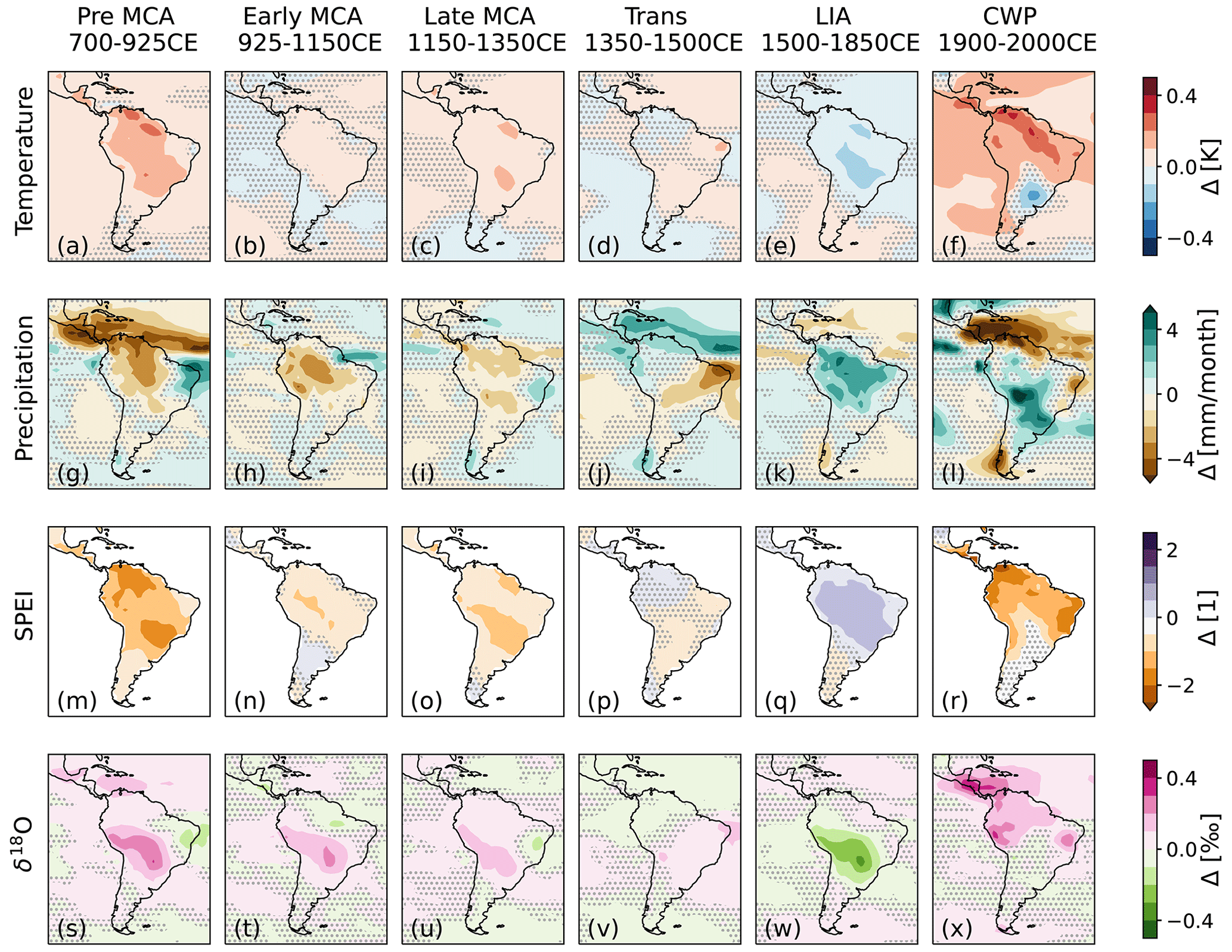
Figure 3 Reconstructed mean anomaly fields for temperature (a–f), precipitation (g–l), SPEI (m–r) and δ¹⁸O (s–x) during five periods with respect to the last-millennium mean (LM, 850–1850 CE). The studied periods are the years preceding the Medieval Climate Anomaly (Pre MCA, 700–925 CE, first column), the early MCA (925–1150 CE, second column), the late MCA (1150–1350 CE, third column), the transition period (Trans, 1350–1500 CE, fourth column), the LIA (1500–1850 CE, fifth column) and the Current Warm Period (CWP, 1900–2000 CE, sixth column). The SPEI values have been standardized using the variance for the period 850–1850 CE. Stippling indicates grid cells where the difference from the last-millennium value is not significant according to Welch’s t test (α>0.01).

We observe in-phase trends for all reconstructed climate variables and studied periods. These generally indicate the simultaneous occurrence of warmer with drier conditions and colder with wetter periods, except during the CWP. Compared to the last millennium mean, the reconstructed CWP anomalies show a more spatially diverse precipitation anomaly field with increased precipitation for the center of the continent. Less precipitation is reconstructed for coastal locations in the north, east and southern margins of the continent. Temperature and SPEI, in contrast, show warmer and drier conditions for the entire continent, except for parts of the La Plata Basin and parts of the Southern Cone. The austral-summer reconstruction (Fig. S4.1), however, shows the largest positive temperature anomaly for the Southern Cone. For both annual and austral-summer reconstructions, the 20th century is warmer and drier than all preceding phases. In terms of spatial homogeneity, the temperature and SPEI anomalies are more extensive compared to the precipitation reconstruction, which has more diverse spatial features. The reconstructed δ¹⁸O of precipitation values for the studied periods change most in the center of the continent, with a trend for the most depleted precipitation to occur during the LIA. The center of the largest changes in the isotopic composition of precipitation is located further to the south than the region with the largest precipitation changes. The δ¹⁸O values of precipitation display a dipole pattern over the Nordeste and central South America except during the more homogeneous MCA–LIA transition period and the CWP, where pronounced δ¹⁸O enrichment is seen for the northern and western parts of the continent.

5.2 South American Summer Monsoon variability

To assess changes in the SASM strength throughout the past 2 millennia, we analyze the mean precipitation anomaly in the core monsoon region as a simplified monsoon index. We use the definition from Vuille et al. (2012), who proposed computing the mean precipitation in the core monsoon region (5–17.5° S/72.5–47.5° W; see the black rectangle in Fig. 1) as an indicator of monsoon strength. Additionally, we further investigate δ¹⁸O, temperature and SPEI changes in the core monsoon region. Figure 4 shows the anomalies from the annual reconstructions in comparison to the reconstructions LMRv2.1 (Tardif et al., 2019) and PHYDA (Steiger et al., 2018). We also performed the reconstruction with subsets of the complete proxy record database, relying on speleothems or tree data only or excluding the speleothems from the complete proxy record database to investigate the effect of using different climate archives.

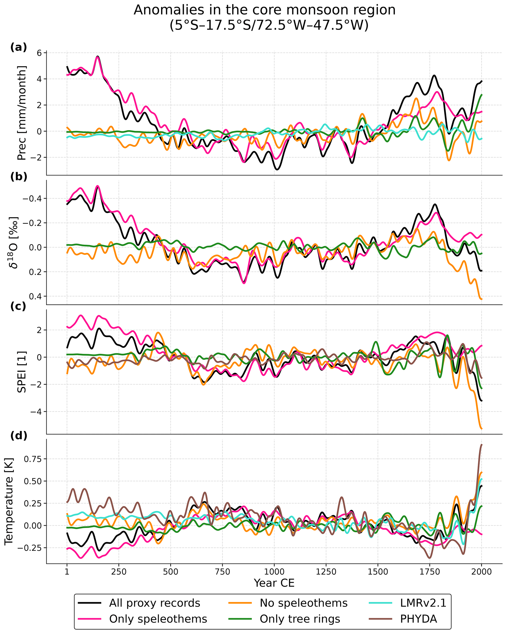
Figure 4 Mean anomalies of precipitation, δ¹⁸O , SPEI and temperature in the core monsoon region (5–17.5° S/72.5–47.5° W). Comparison of reconstructed mean annual precipitation (a), δ¹⁸O (b), SPEI (c) and temperature (d) anomalies in the core monsoon region from reconstructions using all proxy records, excluding the speleothems, using only speleothems or using only trees and from the reconstruction products PHYDA (Steiger et al., 2018) and LMRv2.1 (Tardif et al., 2019). All time series have been smoothed with a 50-year low-pass filter. The anomalies are displayed with respect to the 850–1850 CE mean. Note that the y axis for δ¹⁸O was inverted in order to match the precipitation trend. PHYDA and LMRv2.1 do not include all the variables studied here and are thus partially missing from panels (a), (b) and (c). The SPEI values have been standardized using the variance for the 850–1850 CE period. For the sake of comparability between different reconstructions, we have chosen to display the annual mean reconstruction.

Overall, the reconstructed monsoon index in Fig. 4 and Video Supplements 2 and 3 (Choblet, 2024b and c) show a colder and wetter LIA, particularly after 1500 CE, with anomalies of up to 4 mm per month in the low-pass-filtered curve. The least precipitation is reconstructed for the period from 750–1100 CE, while the SPEI values reach a local minimum earlier (in the period 600–900 CE) and thus seem to more strongly follow the temperature curve, which reaches a local maximum during the same period. Reconstructed temperatures are highest and SASM SPEI values are lowest during the 20th century. This hints that the effects of anthropogenic warming are evident in the core monsoon region on a centennial timescale. Figure 4 shows that the tree-only reconstruction does not reflect the pronounced centennial hydroclimate variability, although the tree ring data represents the dominant climate archive in our proxy record database in terms of numbers. Comparing the reconstruction that exclusively uses speleothem records to the one that excludes speleothems reveals reconstructed hydroclimate changes in the core monsoon region to be largely driven by the speleothem signal. However, wetter LIA conditions are also captured by other archives. The same figure but for the austral-summer reconstruction and the estimates based on all proxies can be found in Fig. S4.5, which exhibits similar trends but larger magnitudes. Furthermore, the smaller reconstruction uncertainty for reconstructions involving speleothems is noticeable, especially compared to the tree-ring-only reconstruction prior to 1400 CE (Fig. S4.6), although the overall uncertainty remains large due to the large spread in the prior ensemble.

Figure 4a additionally displays the LMRv2.1 precipitation reconstruction, which shows lower centennial-scale variations, including no significant changes during MCA, LIA or CWP. Precipitation is not included in the PHYDA reconstruction; however, a comparison of the reconstructed SPEI also indicates less hydroclimate variability during the LIA and the pre-MCA and early-MCA phases. The temperature reconstruction in Fig. 4c shows the largest range of values for the PHYDA reconstruction, followed by the reconstructions of this study and lastly the LMR reconstruction, which shows the least temperature variability. PHYDA shows a constant temperature decline during the CE, with a steep reversal during the 20th century, resulting in the expected hockey-stick-like curve, which is also found in our reconstruction except before 400 CE. The period before 400 CE is peculiar in our reconstruction of all four variables. It shows very wet and cold conditions for the first 2 centuries of the CE and a subsequent transition to more neutral conditions. The reconstructed extremes even exceed the LIA in magnitude.

We note that the presented results draw on the mean values of the MME reconstruction. As is visible in Fig. 5 for the precipitation and Fig. S4.7 for all reconstructed variables, the magnitude of reconstructed change can vary considerably between the single-model reconstructions. It is noticeable that the wet phase prior to 400 CE is particularly pronounced in the isoGSM and ECHAM5 models and is only wetter than the LIA in those two models. For the austral-summer SASM index reconstruction (Fig. S4.5), the range of values for the precipitation anomalies is almost twice as large as for the annual reconstruction, although the overall trends are very similar. Comparing the reconstruction based on all proxy records to the raw prior model simulation without PaleoDA shows that while the model simulations do exhibit larger fluctuations, they do not exhibit clear trends – for instance, a cooler and wetter hydroclimate during the LIA (Fig. S4.8).

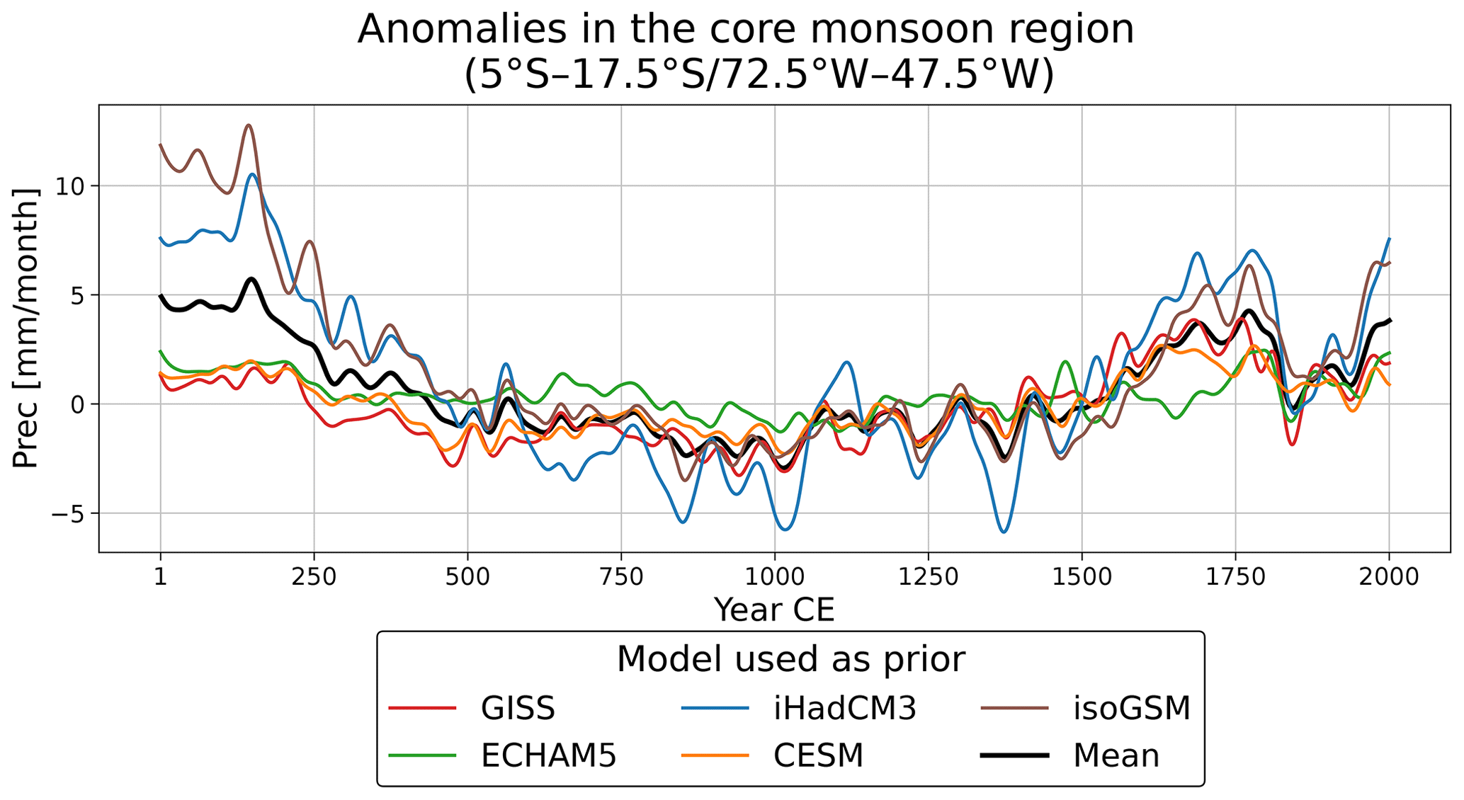
Figure 5 Single-model reconstructions of the monsoon precipitation index using all proxy records, highlighting the prior dependency of the precipitation reconstruction. The black line denotes the multi-model mean, which is used in the multi-model ensemble analysis.

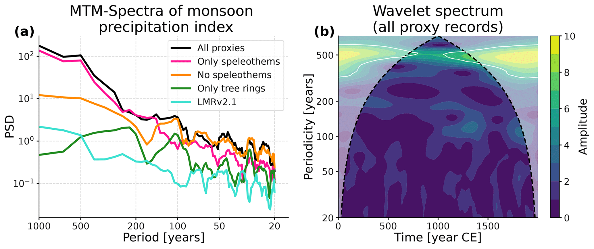
Figure 6 Spectra of the reconstructed monsoon precipitation index. (a) The multitaper method (MTM) – power-spectral densities (PSDs) of the annual reconstructions involving different subsets of the proxy record database. The time series have not been standardized and detrended but have been resampled to 10-year averages to achieve comparability between reconstructions involving different timescales. (b) The continuous-wavelet spectrum for the reconstructed time series involving all proxy records. The dotted black line indicates the cone of influence and the white lines indicate the 95 % significance level for an AR(1) process. All spectra have been computed using the Pyleoclim package in Python (Khider et al., 2022a).

To further study and quantify climate variability in the core monsoon region, we calculated the power-spectral distributions of the precipitation anomaly curves (Fig. 6a). In addition, the continuous-wavelet spectrum of the SASM precipitation reconstruction involving all proxy records was computed to investigate the power variation with time over the Common Era. The same spectral analysis for the reconstructed δ¹⁸O signal in the core monsoon region can be found in Fig. S4.9. The precipitation spectra have typical red-noise characteristics, with the power decreasing exponentially towards higher frequencies, except for the reconstruction based only on tree data, which has a flat power spectrum. The reconstructions that include the speleothems show the highest redness, with a decline in power of over 3 orders of magnitude, as also indicated by the pronounced multi-centennial variability in Fig. 4. Without the speleothems, the power distribution extends over 2 orders of magnitude. The power spectrum of the SASM precipitation anomaly in the LMRv2.1 reconstruction remains flat and is similar to the spectrum for the tree-ring-only reconstruction. The wavelet spectrum of the precipitation reconstruction based on all proxies also exhibits multi-centennial variability of the SASM (Fig. 6b), although it is not above the significance threshold. The spectra for the SASM δ¹⁸O index, which might be represented more directly by the available proxy records, show similar red-noise characteristics (Fig. S4.9). For further comparison, we compared the spectrum of the SASM precipitation index to the spectra of this index in the prior model simulations. To do this, we took into account that the model simulations span a shorter time period than the entire reconstruction period and that they have a higher variance than the reconstruction. The spectra of all five model simulations have a flat shape and thus a smaller variability scaling than the reconstruction (Fig. S4.10).

6 Discussion

6.1 Reconstructed hydroclimate changes

Our climate field reconstruction of the South American hydroclimate during the CE represents a comprehensive synthesis of an encompassing, diverse collection of proxy record data and isotope-enabled climate simulations. The reconstructed centennial climate changes in tropical South America, which transitioned from a drier MCA to a wetter LIA, align well with individual proxy record assessments from the region (Bird et al., 2011; Vuille et al., 2012; Deininger et al., 2019) and proxy record syntheses (Campos et al., 2019; Orrison et al., 2022). This consistency with the conclusions of those studies is expected, given that we used the same (and other) proxy records and the temporal pacing of the reconstruction relies on the information provided by the proxy records within the offline PaleoDA algorithm. We did not perform direct quantitative comparisons between our climate field reconstruction and individual proxy records from single- or multi-proxy studies. This is because speleothem δ¹⁸O values, a proxy for large-scale regional atmospheric behavior, are not expected to agree precisely with the local hydrology. Our reconstruction aims to capture broader regional patterns rather than exact local conditions.

The PaleoDA climate field reconstruction offers the advantage of extrapolating proxy record information to more climate variables, such as temperature from speleothem δ¹⁸O, which in this region is mainly interpreted based solely on precipitation amount changes. The magnitude of reconstructed precipitation amount and SPEI surpass the estimates from the PHYDA and LMRv2.1 reconstructions, while the changes in temperature show similar magnitudes. It is worth noting that the highest temperature anomalies are reconstructed for the period preceding the MCA reference period 950–1250 CE (Fig. 6). This pattern is also observed in the PHYDA and LMR reconstructions (Figs. S4.11 and S4.12), which rely on fewer local proxy record data points from South America for that period. In line with Neukom et al. (2019), South America does not show coherent warming during the MCA compared to other regions globally, which contrasts with the qualitative study by Lüning et al. (2019). Although our reconstruction includes anomalous conditions, their timing might differ from those of the Northern Hemisphere anomalies. Thus, this reference time period should be used with caution in global comparisons.

Another similarity between our reconstruction and PHYDA and LMRv2.1 is the presence of anomalies in the Southern Cone region with opposite signs to those in the northern and central part of the continent. The influence of the Southern Annular Mode in this region may, for instance, cause this distinct opposite climate system. Our reconstruction also reveals a spatial feature over northeastern Brazil, where opposite anomalies in precipitation, drought index and δ¹⁸O are observed compared to the rest of tropical South America. This dipole pattern, previously identified in regional speleothem studies, has been linked to meridional changes in the Hadley cells (Cruz et al., 2009; Novello et al., 2012, 2018) and interhemispheric temperature gradients (Campos et al., 2022). The presence of this dipole pattern in our reconstruction was not necessarily expected, considering the limited number of speleothems from the Nordeste and the relatively coarse spatial resolution of the climate models. In addition, looking into the spatial correlations of the mean δ¹⁸O of precipitation values for that region in the model simulations, we only observe a dipole in two out of the five climate model simulations (Fig. S4.13), thus revealing the benefit of combining proxy and model data with PaleoDA. However, more research for quantifying the extent and possible spatiotemporal variations of the South American δ¹⁸O and the precipitation dipole is required, which should also incorporate additional proxy records from the Nordeste, as we currently only employ two.

A consistent pattern in our hydroclimate reconstruction is the synchronous trend for all variables during most of the CE, except for the 20th century. However, it is essential to acknowledge that the reconstruction technique may also influence this in-phase relationship. Offline PaleoDA with the EnKF, being inherently linear, employs the same static covariance patterns from the simulations at each time step. The in-phase relationship represents the default state of the reconstruction. The increased strength of the SASM during the LIA has been explained by cooler temperatures in the Northern Hemisphere, which result in a southward shift of the ITCZ (Deininger et al., 2019; Vuille et al., 2012). Integrating the proxy records we employed into a global climate field reconstruction and possibly including more atmospheric variables could provide a more in-depth understanding and allow this hypothesis to be tested.

An unexpected finding in our reconstruction is the evidence of wetter and colder conditions prior to 400 CE. The speleothem data mainly support these changes. Upon closer examination of the individual anomalies in the available records in Fig. S4.14, only three records exhibit particularly negative δ¹⁸O anomalies for that period. Furthermore, during that time, proxy records from the margin and outside the core monsoon region are the only available sources. Still, the spatial correlations in the model simulations for the precipitation in the core SASM region prove to be extensive, such that the signal from proxy records outside of the region can influence the reconstructed SASM precipitation (Fig. S4.15). The increased SASM strength stays consistent even after excluding possibly diverging single records that were suspected to cause the anomalies in the reconstruction. While the magnitude of the wet conditions also proved to be model prior dependent, the source of the model differences in reconstruction cannot be directly deduced from the simulated SASM indices and the correlations in the model, requiring further analysis of the topic. In addition to the correlation analysis that we did for the core monsoon region and Nordeste, an optimal sensor placement analysis such as those performed by Comboul et al. (2015) and King et al. (2023) could give insights into how different proxy records influence the reconstruction, depending on the model prior.

6.2 Examining reconstructed trends in relation to single-proxy records

Directing our attention to particularly anomalous proxy records reveals further insights into the nature of our reconstruction. For instance, the record with the strongest negative anomaly, from Paraiso Cave (SISAL-ID 424) in the eastern Amazon Basin (Ward et al., 2019; Azevedo et al., 2019), exhibits a distinctive increase in δ¹⁸O values after 900 CE, resulting in negative δ¹⁸O anomalies during the early Common Era compared to the reference period (1750–1850 CE). This increase may be caused by non-climatic influences, which potentially introduces artifacts into our anomaly reconstruction. The record also stands out in the internal validation procedure (Fig. 2). Nonetheless, this record has been cross-validated with archaeological evidence from the region, which also suggests a shift from wetter conditions in the first millennium to drier conditions in the second millennium (de Souza et al., 2019). In contrast to other speleothem locations in tropical South America, the Paraiso Cave record is additionally influenced by the rainfall of the two distinct systems, SASM and ITCZ. Our PaleoDA approach may not be able to resolve this complex local climate. Different from the drier conditions recorded in Paraiso Cave (Ward et al., 2019), the reconstruction does not show drier conditions during the LIA for the eastern Amazon Basin; it shows wetter conditions, as seen for the entire tropical South America. While this record has a strong influence in the first centuries of the reconstruction, it is outweighed by the multitude of other records during the LIA.

The contrast between the reconstructed wetter and colder climate anomaly fields during the LIA and the information provided by single records highlights the spatial smoothing caused by the PaleoDA method, which we consider the central limitation of our study. The EnKF employs spatial covariances between grid cells and variables in the climate model simulations, which tend to be spatially extensive when computed over the last millennium. As a result, the reconstruction for the eastern Amazon Basin displays wetter conditions because these are the conditions recorded by the majority of the proxy records. While the PaleoDA methodology aims to compute the best climate field estimate from all observations, this example demonstrates that the reconstruction may not always align well with individual observations. This spatial smoothing effect due to the model covariances has been noted in the PaleoDA literature before, e.g., by Sanchez et al. (2021), who focused on the ENSO reconstructed from coral records during the 19th century, or by Erb et al. (2022), who reconstructed the entire Holocene (see the outstanding proxy record anomalies in their Fig. 10). In statistical terms, PaleoDA with the EnKF may cause a loss of spatial degrees of freedom in the reconstruction, which can be expressed in terms of the explained variance of the leading modes obtained via a principal-component analysis (Bretherton et al., 1999). We are not aware of studies investigating climate field reconstructions from the aspect of spatial degrees of freedom, and doing so would be out of scope for this study. However, we note that when investigating spatial temperature correlations of CE reconstructions, Bakker et al. (2022) found larger inter-continental correlations for a PaleoDA reconstruction product compared to other methods (see their Fig. 5). Although our reconstruction product is provided at a spatial resolution of 1.875° × 1.875°, it is more likely to reliably represent spatially extensive regions rather than single grid cells. This aspect is further emphasized by the fact that the climate model simulation data were upsampled to the resolution of the model with the highest spatial resolution. Despite using five different isotope-enabled climate model simulations to mitigate the effect of single-model biases, an ensemble of five models still represents a small ensemble of opportunity. Further, water isotopes have not been included in climate model intercomparison projects, and the number of publicly available simulations is limited to the five models we have employed. The reconstruction would strongly benefit from more isotope-enabled simulations with a variety of models and more up-to-date forcing, such as volcanic forcing (e.g., Sigl et al., 2015). Future PaleoDA reconstructions will also profit from explicitly studying the differences in spatial covariances simulated by the models to potentially discard overly or insufficiently sensitive models (e.g., in the covariance relationship of δ¹⁸O values and precipitation changes). Multi-model reconstructions should further account for similarities between models in the form of weighted ensembles (Eyring et al., 2019). Alternatively, perturbed physics ensembles of isotope-enabled simulations for a single model would allow for larger ensembles and a transient offline PaleoDA approach, as used by Franke et al. (2017) and Valler et al. (2020). The high computational cost of including water isotopes in the simulations currently restrains this type of experiment.

PaleoDA reconstructions that go back deeper in time have also employed prior ensembles that move with time to account for changing boundary conditions and, thus, the non-stationarity of simulated covariances (Osman et al., 2021; Erb et al., 2022). However, the timescales on which covariance patterns of specific hydroclimate variables in the climate system change have not been studied formally yet.

6.3 Multi-decadal hydroclimate variability in the reconstruction

We also studied the reconstructed hydroclimate variability to assess the impacts of different proxy archives, particularly speleothems. The power-spectral distributions of the reconstructed SASM precipitation strength underscore that the use of different climate archives yields distinct hydroclimate variability patterns. Remarkably, the inclusion of speleothems leads to a substantial variability increase on multi-decadal to centennial timescales, contributing to a potentially more realistic reconstruction of the South American hydroclimate.

The significant multi-centennial variability of the SASM (Fig. 6) is comparable to, albeit less pronounced and persistent than, findings in individual speleothem records (Novello et al., 2012; Apaéstegui et al., 2014; Novello et al., 2016; Deininger et al., 2019), where this variability was attributed to solar cycles of 83 and 208 years. However, it is essential to consider that the reconstructed 2000-year time series is probably too short to definitively establish causal relationships for multi-centennial variability. Previous research found only small attributions of solar forcing over the last millennium (Schurer et al., 2013). Future PaleoDA reconstructions using speleothem data may focus on longer reconstruction periods to more thoroughly investigate links to solar forcing. The resemblance between the reconstructed hydroclimate variability in our study and the estimates from single-proxy record studies is expected, given that we use data from these studies as input. However, PaleoDA enables us to underscore the connection between the isotopic composition of precipitation and precipitation amount. Moreover, spectral analyses derived from proxy record compilations generally yield more reliable estimates of hydroclimate variability.

Our study did not explicitly aim to compare the hydroclimate variability in the reconstruction with that in climate model simulations. However, initial analyses reveal a more pronounced multi-decadal to centennial hydroclimate variability in the reconstruction, corroborating previous model–data comparisons for speleothems and isotope-enabled climate models. For tropical South America, Orrison et al. (2022) demonstrated that the GISS and iCESM last-millennium simulations underestimate centennial monsoon intensity changes in the isotopic composition of precipitation. On a global scale, Bühler et al. (2021) found an underestimation of multi-decadal to centennial variability when using climate simulations that were also included in our study. A similar underestimation of multi-decadal to centennial variability was previously found for precipitation in the CMIP5 last-millennium ensemble for tropical South America (Parsons et al., 2018) and globally (Ault et al., 2012; Parsons et al., 2017), where the spectra were shown to resemble the spectrum of white noise. Additionally, for temperature, it is now established that while climate models generally capture the climate variability of global mean temperature, they underestimate regional temperature variability (Laepple et al., 2023b). Our PaleoDA reconstruction, thus, represents a compromise between climate models and climate proxy records, potentially providing a more realistic representation of hydroclimate variability scaling than models alone. We emphasize that the reconstruction of multi-decadal to centennial variability would not have been feasible without the multi-timescale PaleoDA approach, which enables the inclusion of speleothems primarily for technical reasons. It remains to be determined if the use of multi-year covariances, instead of annual ones, in the PaleoDA algorithm also contributed to this, as is suggested by pseudoproxy experiments (Steiger and Hakim, 2016; Choblet et al., 2023). However, this matter is beyond the scope of this publication.

In principle, our reconstruction could be employed to investigate interannual variations in SASM strength, for which the ENSO is considered a driver (Garreaud et al., 2009). However, we only employed the key archive for SASM variability, the speleothems, at decadal resolution, even though many of the records technically have finer resolution. The conservative approach of using decadal timescales for speleothems was adopted to avoid additional complexity arising from dating uncertainty, sampling from age-model ensembles during the reconstruction and the need to take into account the transit time of cave seepage water. Developing a scheme that considers all these factors would enable the influence of the ENSO on SASM variability to be studied. Employing speleothems at higher resolutions might also improve validation results against 20th-century instrumental precipitation in the region.

6.4 Future developments

The PaleoDA reconstruction could be enhanced by exploring more elaborate PSMs that perform absolute-value reconstructions instead of anomaly reconstructions. In previous work leading up to this study, the speleothem PSM proposed by Dee et al. (2015) was tested but did not reduce offsets between models and proxy records. This can result from either model biases, PSMs that do not incorporate processes known to a local cave expert or a lack of physical understanding of the records. Therefore, we compared simulation and proxy record anomalies by taking known seasonality into account or via a linear regression for tree and coral time series. For speleothems, including information from local cave-monitoring studies (e.g., Moquet et al., 2016; Sekhon et al., 2021; Jiménez-Iñiguez et al., 2022), could provide a better understanding of the proxy record and help recognize model biases in simulated δ¹⁸O of precipitation values as well as improve PSMs. However, this usually requires more metadata for individual cave systems, which are not always available, and may reduce the number of usable proxy records.

When employing more elaborate PSMs in PaleoDA, it is essential to test their effect on the covariance patterns, as nonlinear mathematical operations can impact covariances unexpectedly. Applying PSMs of higher complexity to instrumental data could also improve the assessment of the proxy error and SNR. Although we consider the employed SNR of 0.5 reasonable, it remains a broad assumption due to the lack of sufficiently long instrumental time series at the cave locations. Previous PaleoDA reconstructions without clear proxy record errors have used a post hoc adjustment of the error variance (Tierney et al., 2020; Osman et al., 2021). However, we refrain from doing so here, as the tuned errors might be confounded by model biases in the covariances, and the proxy record error should represent a real physical and statistical property rather than a tunable hyperparameter. An alternative reconstruction that set the proxy record variance equal to the prior record variance yielded similar climate fields with more pronounced magnitudes of hydroclimatic changes (Fig. S4.2). Due to this similarity, we have not investigated these reconstructions further, but we emphasize that, in the light of the unclear SNRs of speleothems and other proxy records, an equal prior/proxy weighting approach would be equally legitimate.

7 Conclusion

This study presents the first South American climate field reconstruction for the entire CE and the entire continent. By incorporating speleothems and other non-annually resolved climate archives through a multi-timescale data assimilation approach, we have improved the spatial proxy record coverage for South America compared to previous global reconstructions and eliminated the need for the uncertain calibration of low-resolution isotopic records to temperature and precipitation. Our primary focus was centered on centennial climate changes, with particular attention paid to the intensity of the SASM. The reconstruction reveals compelling evidence of a strengthened monsoon during the LIA, contrasting with a weaker SASM before, in particular during the early phase of the MCA. We also found a strengthening during the first centuries of the CE, which remains more elusive due to the more limited number of proxy records. In our reconstruction, speleothems played a vital role in capturing centennial variability. While this study showcases the potential of the multi-timescale PaleoDA reconstruction approach that includes speleothems, we acknowledge certain limitations that warrant further investigation. Uncertainties in proxy record errors, spatial smoothing of the reconstruction and the necessity for a larger ensemble of isotope-enabled climate model simulations with diverse models are important areas for future research. Particular emphasis must be placed on improving the validation of multi-timescale PaleoDA reconstructions based on low-resolution proxy records such as speleothems, as this proves to be particularly challenging due to a lack of instrumental data. Our work relies on the assumption that speleothem δ¹⁸O values indicate large-scale precipitation changes. This assumption will benefit from further validation, particularly through the analysis of speleothem records that reliably capture SASM fluctuations at sub-decadal timescales. The establishment of validation protocols will further help in better assessing the reconstruction skill of multi-timescale PaleoDA reconstructions. Additionally, the exploration of differences in simulated covariance patterns – which are fundamental to the PaleoDA EnKF reconstruction algorithm – holds promise for refining and enhancing this methodological approach. We make our reconstructed datasets publicly available, providing a foundation for future climatological data analysis, including comparisons to proxy records, other reconstructions and climate simulations. Furthermore, by publishing the code for the multi-timescale PaleoDA algorithm alongside this study, we encourage and enable the application of the multi-timescale PaleoDA method to proxy records of different temporal resolutions. This concept has great potential for global climate field reconstructions, particularly for the CE and older time periods, where speleothems and other non-annually and irregularly resolved proxy records serve as essential indicators of past hydroclimate changes.