Modelling Mediterranean ocean biogeochemistry of the Last Glacial Maximum

We present results of simulations performed with a physical–biogeochemical ocean model of the Mediterranean Sea for the Last Glacial Maximum (LGM) and analyse the differences in physical and biochemical states between the historical period and the LGM. Long-term simulations with an Earth system model based on ice sheet reconstructions provide the necessary atmospheric forcing data, oceanic boundary conditions at the entrance to the Mediterranean Sea, and river discharge to the entire basin. Our regional model accounts for changes in bathymetry due to ice sheet volume changes, reduction in atmospheric CO₂ concentration, and an adjusted aeolian dust and iron deposition. The physical ocean state of the Mediterranean during the LGM shows a reduced baroclinic water exchange at the Strait of Gibraltar, a more sluggish zonal overturning circulation, and the relocation of intermediate and deep-water-formation areas – all in line with estimates from palaeo-sediment records or previous modelling efforts. Most striking features of the biogeochemical realm are a reduction in the net primary production, an accumulation of nutrients below the euphotic zone, and an increase in the organic matter deposition at the seafloor. This seeming contradiction of increased organic matter deposition and decreased net primary production challenges our view of possible changes in surface biological processes during the LGM. We attribute the origin of a reduced net primary production to the interplay of increased stability of the upper water column, changed zonal water transport at intermediate depths, and lower water temperatures, which slow down all biological processes during the LGM. Cold water temperatures also affect the remineralisation rates of organic material, which explains the simulated increase in the organic matter deposition, which is in good agreement with sediment proxy records. In addition, we discuss changes in an artificial tracer which captures the surface ocean temperature signal during organic matter production. A shifted seasonality of the biological production in the LGM leads to a difference in the recording of the climate signal by this artificial tracer of up to 1 K. This could be of relevance for the interpretation of proxy records like, e.g., alkenones. Our study not only provides the first consistent insights into the biogeochemistry of the glacial Mediterranean Sea but will also serve as the starting point for transient simulations of the last deglaciation.

1 Introduction

The Earth climate during the Last Glacial Maximum (LGM) was characterised by much colder climate conditions and the existence of massive ice sheets in the Northern Hemisphere which led to a lowering of the sea level by 70–130 m (Lambeck et al., 2014; Peltier et al., 2015; Tarasov et al., 2012) and significant changes in the atmospheric and oceanic circulation (Löfverström and Lora, 2017), including changes in precipitation and temperature patterns (Kageyama et al., 2021; Löfverström, 2020). These global variations also affect the physical and biogeochemical states of the semi-enclosed Mediterranean Sea (MedSea) which is connected to the global ocean at the Strait of Gibraltar. Today's typical anti-estuarine thermohaline zonal overturning circulation (ZOC) with fresher and nutrient-poor water entering at the Strait of Gibraltar and a salty and nutrient-enriched deeper return flow of primarily Levantine intermediate water masses was slowed down during the LGM (Mikolajewicz, 2011; Colin et al., 2021). Modelling studies indicated that the primary causes of the ZOC variation are the reduced throughflow area at the Strait of Gibraltar at low sea level stands (Mikolajewicz, 2011; Colin et al., 2021) and an increased water column stability hampering the formation of Levantine intermediate water (Rohling, 1991; Mikolajewicz, 2011). Water mass proxy data recorded in foraminiferal authigenic fraction confirm the reduced water exchange during the LGM between the eastern and the western MedSea basins (Duhamel et al., 2020; Cornuault et al., 2018) and point towards a strong salinity increase in the eastern basin (Thunell and Williams, 1989). The globally more arid LGM climate would support higher salinities, but colder conditions also reduce evaporative fluxes. The net water loss of the MedSea for the LGM is approximately only half of that for modern times (Mikolajewicz, 2011). Tendencies of precipitation and river runoff at the LGM are rather uncertain. A multi-model analysis of palaeo-simulations with Earth system models (Kageyama et al., 2021) showed a local precipitation increase over the MedSea, which is also supported by the study of Goldsmith et al. (2017) on long-term water isotopic composition over Israel. In contrast, pollen records concordantly suggest the expansion of steppe vegetation and thus significant aridification during the LGM (Allen et al., 1999; Kotthoff et al., 2008; Koutsodendris et al., 2023), and sediment core data which capture climate changes in the Nile catchment rather indicate arid conditions and reduced river discharge compared to the present (Box et al., 2011; Revel et al., 2014).

While there are a small number of modelling attempts to reconstruct the physical ocean of the MedSea during the LGM (Myers et al., 1998; Rohling and Gieskes, 1989; Mikolajewicz, 2011), there are none at all published for the glacial biogeochemical conditions of the MedSea. Thus, our understanding of the tendencies of biogeochemical tracers between past and present stems solely from the interpretation of sediment core data. Late glacial faunal records from benthic foraminifers indicate that organic matter flux to the seafloor during the LGM was significantly higher than today (Kuhnt et al., 2007; Abu-Zied et al., 2008; Schmiedl et al., 2010). Commonly, it is widely assumed that organic matter fluxes to the seafloor in oligotrophic regions without oxygen limitations are highly correlated to surface primary production (Betzer et al., 1984). As an example, for the present-day MedSea, the decreasing primary production from the western to the eastern basin and the concurrent resulting decrease in food availability at the seafloor is clearly reflected in the benthic foraminiferal composition (Rijk et al., 2000). Consequently, an enhanced organic matter flux during the cold period would point to a higher primary production quantified, for example, for a single sediment core in the western MedSea (Alboran Sea), which shows a 10 % increase in annual primary production (Radi and de Vernal, 2008). Benthic foraminiferal stable carbon isotope records suggest approximately 20 % higher glacial primary productivity in the Ligurian Sea but no significant changes in the Strait of Sicily (Theodor, 2016).

Increased LGM primary production due to upward mixing of nutrients into the euphotic layer was also postulated by Rohling and coworkers (Rohling and Gieskes, 1989; Rohling, 1991), based on theoretical considerations about a shallowing of the pycnocline position in the eastern basin. However, changes in surface nutrient supply during the LGM are still unclear, which impedes also the interpretation of sediment core data. We present the results of a new model framework (medHAMOCC) to investigate the physical and biogeochemical conditions in the MedSea during the LGM. The setup consists of a regional ocean–biogeochemical model for the MedSea which is forced by unique new data sets from an Earth system model (Max Planck Institute Earth System Model, MPIESM) suitable for long-term palaeo-simulations (Kapsch et al., 2022). The MPIESM provides all necessary atmospheric and lateral oceanic physical boundary conditions and river runoff from the last glacial to the present day (26 000 years) for two different ice sheet reconstructions (see Sect. 2.2). With these consistent data sets, we investigate the mean state of the MedSea for two time slices, namely the LGM and present day. We also consider changes in bathymetry and in nutrient river loads for the LGM. The efficient performance of the regional MedSea model allows a 1000-year spin-up run followed by a 1000-year simulation for each time slice. This guarantees a very low model drift and also minimises the impact of initial conditions. Following a model evaluation of present-day conditions (Sect. 3), we address the drivers of circulation changes between past and present and analyse their impact on the biogeochemistry in detail (Sect. 4). An additional sensitivity run is performed to gain further insights into the impact of a changed LGM bathymetry (Sect. 2.3). By introducing a diagnostic tracer to track biological production temperatures, we mimic the information captured in palaeo-proxy data records. This gives us the opportunity to investigate potential biases that may occur when recording the climate signal in marine sediment cores (Sect. 4.4). Future applications and limitations of our model framework will be discussed at the end of this paper (Sect. 5).

2 Methods

2.1 Model setup

We use a regional setup of the primitive equation ocean general circulation model MPIOM (Mikolajewicz, 2011; Jungclaus et al., 2013; Mauritsen et al., 2019) coupled with a comprehensive biogeochemical model HAMOCC (Six and Maier-Reimer, 1996; Ilyina et al., 2013) in an updated version of the one used by Liu et al. (2021). This setup is called medHAMOCC in the following. MPIOM is formulated on an Arakawa C grid in the horizontal and on z levels in the vertical direction using the hydrostatic and Boussinesq approximations. Subgrid-scale parameterisations include lateral mixing on isopycnals (Redi, 1982) and tracer transports by unresolved eddies (Gent et al., 1995). Vertical mixing is realised by a combination of the Richardson-number-dependent scheme of Pacanowski and Philander (1981) and direct wind-driven turbulent mixing in the mixed layer (further details are given in  Jungclaus et al., 2013; Mauritsen et al., 2019). The Mediterranean setup of the MPIOM covers the entire Mediterranean Sea and the Black Sea (Fig. 1). Part of the Atlantic is included as a sponge zone for the open western boundary (see Sect. 2.2). The numerical grid has a mean horizontal resolution of approx. 20 km and 42 unevenly distributed layers in the vertical (9 layers in the upper 100 m and increasing layer thicknesses to a maximum and constant layer thickness of 150 m below 675 m). The bathymetries for the present day and Last Glacial Maximum are derived from ice sheet reconstructions, following the method of Meccia and Mikolajewicz (2018). We consider partial grid cells in the last wet grid cell. Figure 1 shows the present-day land–sea mask and basin depth. The overlaid LGM shoreline indicates a closed Bosporus gateway and the desiccation of the northern Adriatic Sea due to low sea level stands (see Sect. 2.3). The same hydrodynamic processes that are resolved for tracers within MPIOM are applied to all tracers of the biogeochemical component HAMOCC (Six and Maier-Reimer, 1996; Ilyina et al., 2013; Paulsen et al., 2017). HAMOCC includes a description of the full carbon chemistry, the cycling of nutrients (phosphate, nitrate, silicate, and iron) and oxygen, and a plankton dynamics with five tracers (two types of phytoplankton, bulk and nitrogen fixers, one zooplankton type, and dissolved and particulate organic matter, with the latter called detritus). Phytoplankton growth depends on incoming light at the corresponding depth level, the availability of nutrients, and temperature (Paulsen et al., 2017). HAMOCC includes detritus settling and remineralisation of dissolved organic matter and detritus (aerobic and anaerobic), as well as the production, gravitational sinking, and dissolution of opal and calcite shells (Ilyina et al., 2013; Mauritsen et al., 2019). Shell production is linked to plankton concentration changes, with a preference for opal production as long as silicate is available (Ilyina et al., 2013). Organic matter from primary production is composed of carbon, phosphorus, nitrogen, and oxygen, according to a constant stoichiometry (C:N:P:O${}_{\mathrm{2}}=\mathrm{122}:\mathrm{16}:\mathrm{1}:-\mathrm{172}$; Takahashi et al., 1985), and iron (Fe: P$=\mathrm{366}\times {\mathrm{10}}^{-\mathrm{6}}$; Johnson et al., 1997). A sediment module, which consists of solid components (detritus, opal and calcite shells, clay, and sand), includes the same remineralisation and dissolution processes in porewater as in the water column and acts as the lower boundary (Heinze et al., 1999). The sediment module has the same horizontal resolution as medHAMOCC and 12 biologically active levels with increasing layer thickness and decreasing porosity from the water–sediment interface to a diagenetically consolidated burial layer.

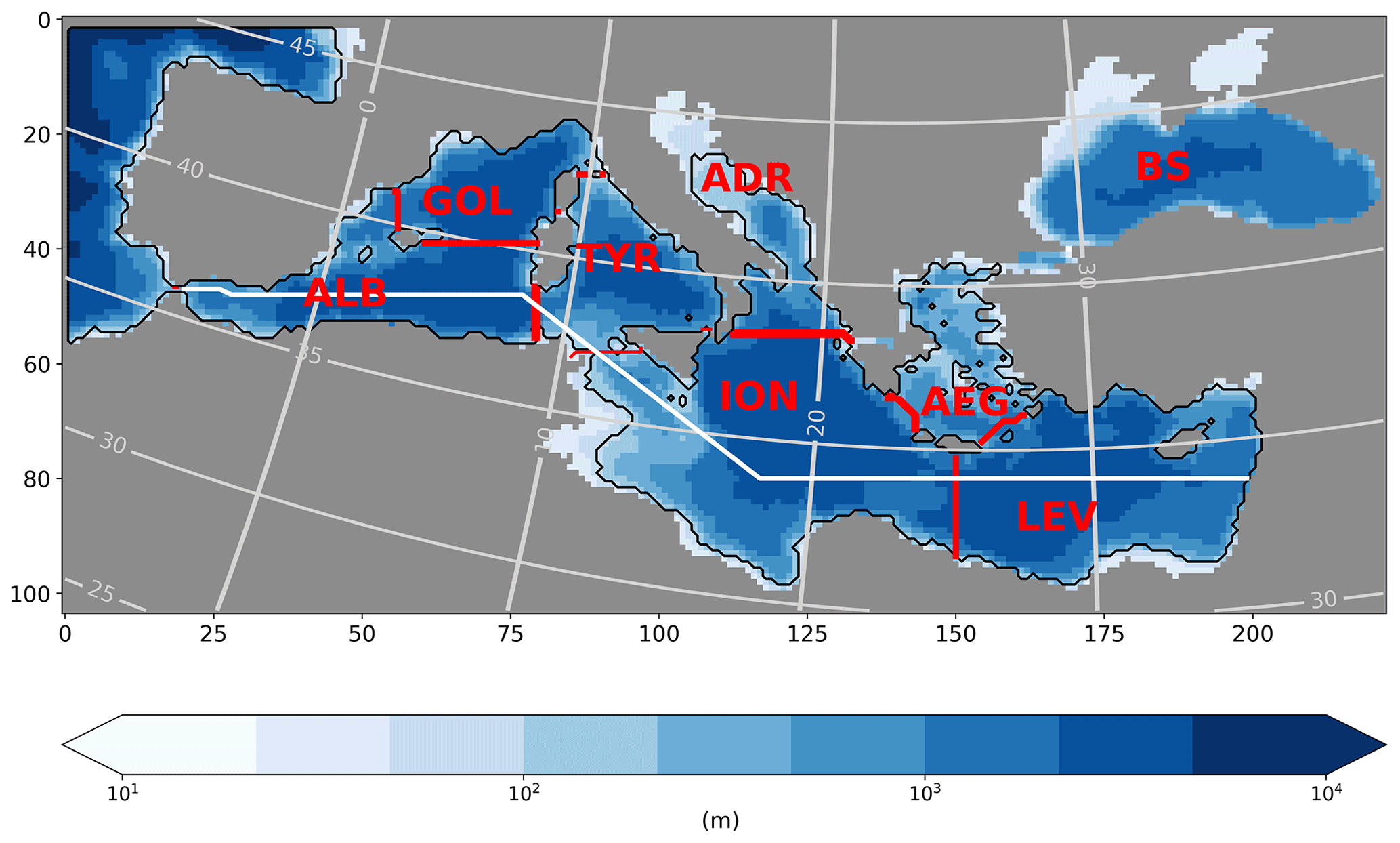
Figure 1 Topography of the present day (depth in m) for the entire model domain (225×104 grid cells). LGM shoreline is given by the black contour line. Light grey lines give the corresponding longitudes and latitudes. Red lines indicate the extension of regions used for basin averages: ALB is for Alboran, GOL is for Gulf of Lion, TYR is for Tyrrhenian Sea, ION is for Ionian Sea, LEV is for Levantine Sea, AEG is for Aegean Sea, ADR is for Adriatic, and BS is for Black Sea. The white line shows the geographical location of the west–east section.

Two major changes have been introduced in the here-applied medHAMOCC compared to the latest version of HAMOCC6 (Mauritsen et al., 2019):

1. A modified sinking and remineralisation process of detritus. In general, gravitationally driven detritus fluxes show the shape of a power law function (Martin et al., 1987). Variations in the settling velocity, which are attributed to disaggregation and aggregation of particles or changes in the intensity of remineralisation, e.g. due to temperature-dependent bacterial activity, form this curve (Kriest and Oschlies, 2008; Laufkötter et al., 2017). As the exponent of the power law function is given by the ratio of the remineralisation rate and the particle settling velocity, a decrease in the remineralisation rate has the same effect on the exponent as an increase in the settling velocity (Kriest and Oschlies, 2008). In HAMOCC6, a depth-dependent detritus sinking speed and a temperature-independent remineralisation rate are applied. In view of the large temperature difference between the LGM and present day, we introduce a temperature-dependent remineralisation rate (Bidle et al., 2002) and a constant detritus sinking speed in medHAMOCC. The control parameters were optimised to obtain an equivalent result between the two parameterisation approaches for the present day. Note that the remineralisation rate is oxygen-dependent in both HAMOCC versions.

2. A sediment resuspension. We implemented the sediment resuspension scheme developed in Mathis et al. (2019). Depending on the grain size, particle density, and bottom-shear stress, all solid particles (except for sand) from the uppermost sediment layer can be remobilised and are relocated or remineralised in the water column.

Additionally, we introduce a tracer (T_org) to track the temperature at which primary production takes place. T_org, a kind of a phytoplankton twin, is treated by the same biological turnover processes and eventually enters the sediment by organic matter settling. It mimics the information which is implicitly carried by proxy data, such as alkenones. T_org gives us the possibility for assessing the potential biases that may occur when climate signals are recorded by proxy data.

2.2 Forcing and boundary conditions

All necessary atmospheric forcing fields are taken from long-term palaeo-simulations with an Earth system model (MPIESM; Kapsch et al., 2022). These transient simulations cover the entire period from the last glacial to present day (26 000 years), but we use only two time slices here, namely the LGM and the preindustrial period (PI). To allow a consistent spin-up, we take 2000 years of transient forcing data for each time slice, LGM (22 000–20 000 yr BP) and PI (2000–0 yr BP; reference year 1950), and we consider the first 1000 years of each time slice simulation as spin-up. Atmospheric forcing data are 2 m temperature, dew point temperature, downward short- and longwave radiation, 10 m wind speed, zonal and meridional wind stress components, and precipitation as monthly averages. The atmospheric model component of MPIESM has a relatively coarse horizontal resolution (approx. 3.75°). Therefore, we applied a simple downscaling procedure with bias correction on the basis of reanalysis data (ERA 20C; Poli et al., 2016). Heat and freshwater fluxes over the water are calculated using the standard bulk formulae (Mikolajewicz, 2011; Liu et al., 2021).

A unique feature of these long-term simulations with MPIESM is an automatic adaptation of the topography/bathymetry due to volume changes in ice sheets and isostatic adjustment which is calculated every 10 simulation years (Kapsch et al., 2022). Corresponding changes in the hydrological discharge and the river routing are also considered (Riddick et al., 2018). For medHAMOCC, we adopt the same automatic adaptation of the topography/bathymetry and consider the transient hydrological discharge to the MedSea. We add freshwater from the river runoff with a corresponding nutrient load (phosphate, nitrate, and silicate). This nutrient load is deduced from simulated freshwater discharge multiplied by a mean river nutrient concentration for individual basins of the Mediterranean Sea and the Black Sea to account for temporal variability in the nutrient supply. We derive the basin mean nutrient concentration from modern nutrient input estimates (Ludwig et al., 2009) divided by the simulated mean basin river discharge of the last 10 years of the MPIESM simulation. This procedure guarantees a realistic nutrient supply for the present day, despite a potential river discharge bias in the parent simulation. Aeolian clay and iron deposition for the PI and the LGM are taken from Albani et al. (2016).

Tarasov et al. (2012)Tarasov et al. (2012)Peltier et al. (2015)Peltier et al. (2015)Tarasov et al. (2012)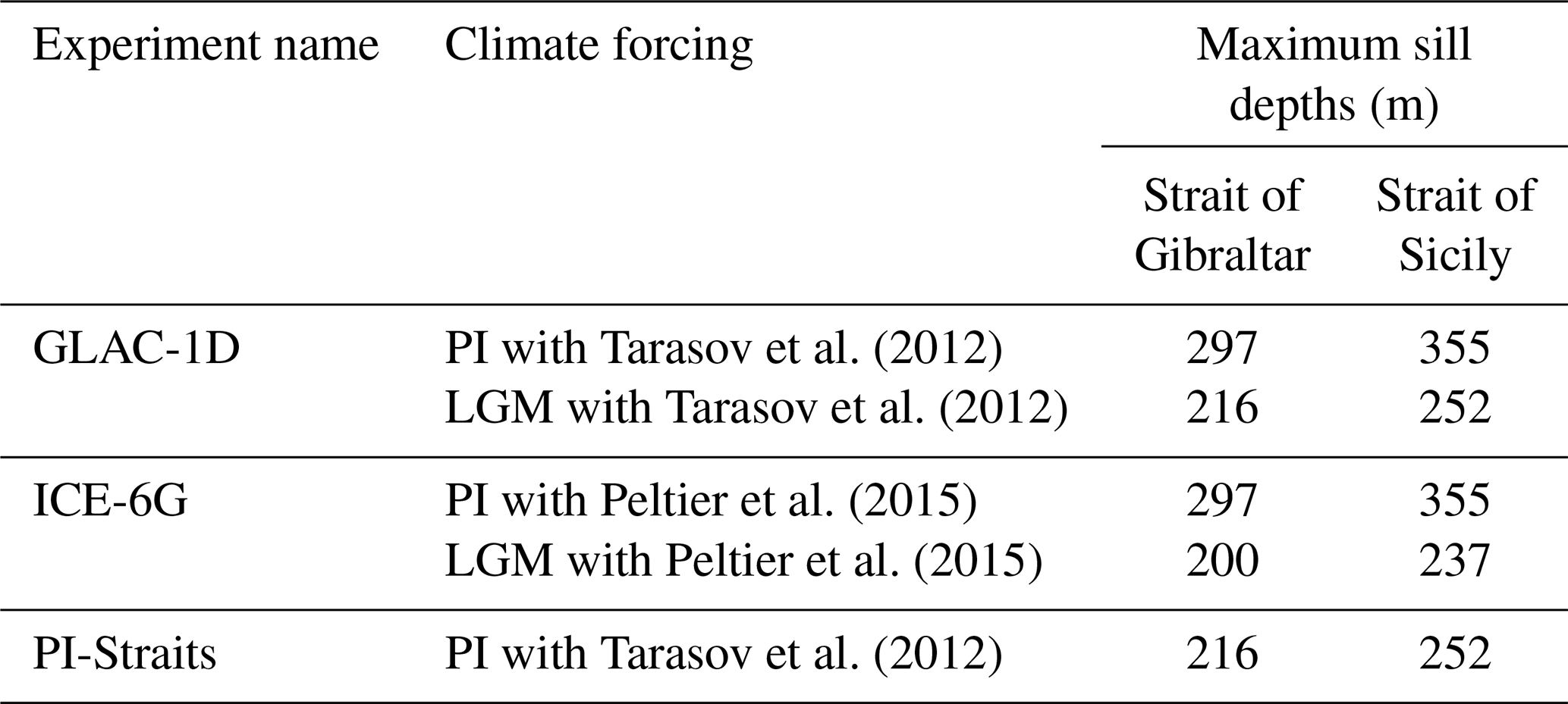

Table 1 List of experiments and their major differences.

The northern/western boundary of the model domain in the Atlantic Ocean is a solid wall with an adjacent sponge zone of about 80 km over which ocean temperatures and salinities are relaxed to the corresponding monthly mean data from the MPIESM simulation with a relaxation time of 1 month. These boundary conditions of MPIESM have been bias-corrected by the difference between the mean of the last 100 years of the MPIESM simulation and the Polar Science Center Hydrographic Climatology for temperature and salinity (Steele et al., 2001). To guarantee a nearly constant water volume in the model domain and a consistent water flux at the Strait of Gibraltar, the sea level is relaxed to zero in the sponge zone. All biological organic components (e.g. phytoplankton) are relaxed to their prescribed minimum concentration. For other biogeochemical tracers, we use climatological monthly mean data from the World Ocean Atlas (phosphate, nitrate, oxygen, and silicate; Garcia et al., 2019a, b) and climatological annual mean data from GLODAPV2 (dissolved inorganic carbon and alkalinity; Lauvset et al., 2021). We are aware of the inconsistency with respect to prescribing modern concentrations in the sponge zone in a LGM simulation. However, estimates of the nutrient concentrations for the LGM remain a challenge. Tamburini and Föllmi (2009) suggested an overall increase in the global phosphate inventory of 17 %–40 % between the LGM and present day. Some sediment records along the Iberian margins (Kohfeld et al., 2005; Radi and de Vernal, 2008) and a few modelling studies (Bopp et al., 2003; Menviel et al., 2008; Palastanga et al., 2013) point towards higher export production in the eastern side of North Atlantic between 0–40° N as a result of enhanced nutrient upwelling and/or nutrient supply from shelf areas due to sea level low stands. However, a higher global phosphate inventory does not imply that surface nutrient concentrations are also higher in the North Atlantic (Bopp et al., 2003; Morée et al., 2021) and that more nutrients would enter the Mediterranean Sea. Therefore, we stick to the present day's values for the prescribed boundary conditions in the sponge zone.

2.3 Set of experiments

From MPIESM, we use forcing data sets from two simulations based on different ice sheet reconstructions (GLAC-1D, Tarasov et al., 2012; ICE-6G, Peltier et al., 2015; see Table 1). Differences in these “parent” simulations arise primarily from the temporal change in ice volume and its impact on the atmospheric circulation, as well as the freshwater discharge from ice melt affecting sea surface salinity and, consequently, ocean meridional overturning circulation in the North Atlantic (Kapsch et al., 2022). Estimates of different ice sheet volumes during the LGM for GLAC-1D and ICE-6G lead to different eustatic sea level changes of about 70 and 100 m, respectively. Consequently, the present-day sill depth at the Strait of Gibraltar (297 m) shallows to 216 m in GLAC-1D and 200 m in ICE-6G. By applying forcings from different ice sheet reconstructions, we capture uncertainties resulting from glacial boundary conditions. Each parent simulation provides 2000 years of a consistent forcing for the LGM (22 000–20 000 yr BP) and preindustrial (2000–0 yr BP, with a reference year of 1950) time slices. Our results are shown as means for the last 1000 years of each simulation, with an exception for the model–data comparison with MEDATLAS (MEDAR Group, 2002) as we use only the last 70 years of the PI simulation of GLAC-1D and ICE-6G.

In addition, we perform a sensitivity study with the present-day GLAC-1D forcing to assess only the impact of shallower sill depths of the Strait of Gibraltar and of the Strait of Sicily on the circulation of the MedSea. To this end, we reduce the sill depth of the Strait of Gibraltar and the Strait of Sicily to LGM values (216 m for the Strait of Gibraltar and 252 m for the Strait of Sicily) in the experiment PI-Straits (Table 1). The remaining bathymetry is unchanged.

3 Assessment of the physical and biogeochemical state of the PI

Before we discuss the LGM results, we briefly assess the performance of the physical and biogeochemical state for the PI simulations. Both simulations show very similar results for temperature and salinity for the PI, which is attributable to the very similar PI states of the parent simulations. The basin-wide average of temperature for the Gulf of Lion (GOL; Fig. 2a) agrees quite well with the data compilation of MEDATLAS (MEDAR Group, 2002), but the model results are slightly too cold for the Levantine basin (LEV; Fig. 2e). Both mean salinities of the basins are fresher (0.2–0.6) compared to the observations, but the simulated surface salinity difference between GOL and LEV (0.76–0.82) is comparable to the observed one (approx. 1). Note that we used only the last 70 years of the PI simulations for this model–data comparison.

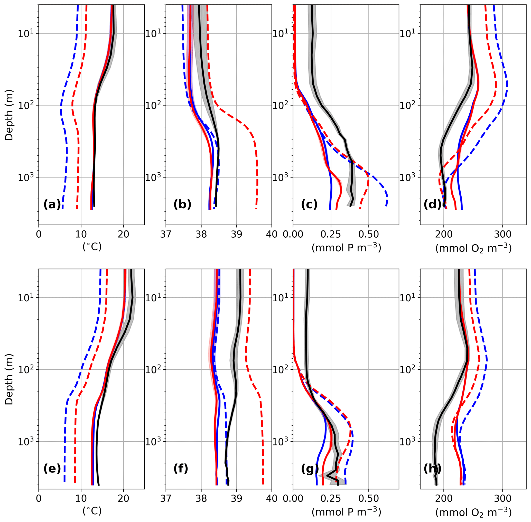
Figure 2 Basin-wide averages for temperature (a, e; °C), salinity (b, f), phosphate (c, g; mmol P m⁻³), and oxygen (d, h; mmol O₂ m⁻³) for the Gulf of Lion (GOL; a–d) and the Levantine (LEV; e–h) for GLAC-1D (blue) and ICE-6G (red). Solid lines refer to the PI and dashed lines to the LGM. The black line indicates basin-wide averages of observations (MEDAR Group, 2002), including their standard deviations (grey shading). For this comparison to observations, we averaged only over the last 70 years of the PI simulations. Note the logarithmic depth axes. See Fig. 1 for basin definitions.

Table 2 Hydrological budget of the Mediterranean Sea for present day from observations (OBS; Sanchez-Gomez et al., 2011) and of PI and LGM for GLAC-1D and ICE-6G. Numbers are given in 1000 m³ s⁻¹. For OBS, numbers are converted (from mm yr⁻¹) for an area of the Mediterranean with 2.5×10¹² m². Numbers in parentheses for river runoff give the Black Sea contribution for PI. The Bosporus gateway is closed during the LGM.

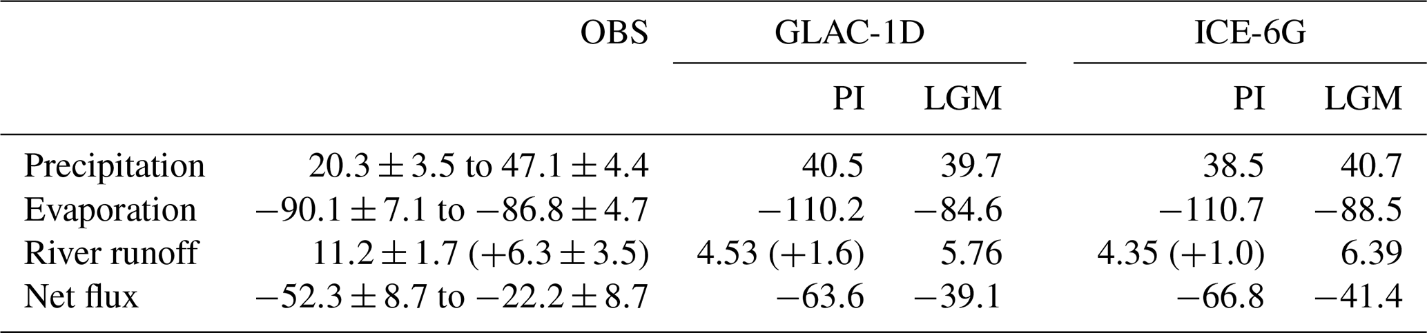
The MedSea is an evaporative basin in which evaporation exceeds precipitation and river input ($\text{PR-E}=\mathrm{precipitation}+\mathrm{river}\mathrm{runoff}-\mathrm{evaporation}$). Surface salinities are the result of the interplay between the net water budget, basin water residence time, and the salinity signal of inflowing North Atlantic water. Simulated absolute PR-E (63–67×1000 m³ s⁻¹ in both PI simulations) is slightly higher than observational estimates (22–52×1000 m³ s⁻¹; Rohling et al., 2015, and references therein; Sanchez-Gomez et al., 2011), and simulated river runoff to the entire MedSea, including the Black Sea contribution at the Bosporus (in total about 5–6×1000 m³ s⁻¹), is much lower than the observational estimates (Dubois et al., 2011: 17.5×1000 m³ s⁻¹; Ludwig et al., 2009: 13.6–23.3×1000 m³ s⁻¹) (Table 2). Our atmospheric parent model, which has a very coarse horizontal resolution (3.75°), potentially underestimates the total runoff to the entire region, as already shown for MPIESM model versions with even higher spatial resolution (Sanchez-Gomez et al., 2011). The net water loss through evaporation is compensated by a net inflow of Atlantic water (+0.06–0.076 Sv; 1 Sv =10⁶ m³ s⁻¹) which is within the range of observational estimates (+0.04–0.11 Sv; Candela, 2001; Tsimplis and Bryden, 2000).

Figure 3 shows the individual in- and outflow contributions for PI which are 1.15–1.25 Sv at the upper end of the range of estimates (e.g. for the outflow; Tsimplis and Bryden (2000): 0.78 Sv; Candela (2001): 0.97 Sv; Lacombe and Richez (1982): 1.15 Sv). The simulated net heat budget (−6 to −4 W m⁻²) compares well to the observational estimates (−7 to −1 W m⁻²; Dubois et al., 2011) (Table 3).

Table 3 Annual mean heat fluxes of the Mediterranean Sea (W m⁻²) from observations (OBS; Sanchez-Gomez et al., 2011) and of PI and LGM for GLAC-1D and ICE-6G.

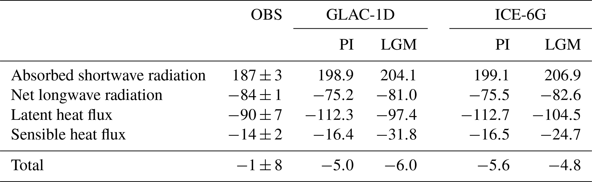
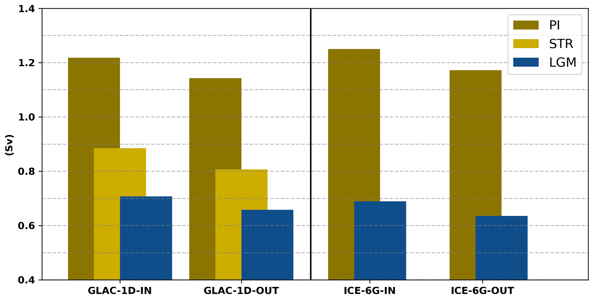
Figure 3 Baroclinic water transport (Sv) at the Strait of Gibraltar separated into in- and outflow components for the PI (brown bars) and LGM (blue bars) of GLAC-1D and ICE-6G. Golden bars indicate the results of PI-Straits (STR). See also the legend in the upper-right corner.

The simulated thermohaline circulation shows the characteristic clockwise zonal overturning pattern between 5° W and 25° E in the upper 1000 m, with a maximum strength of more than 1 Sv for the PI (Fig. 4), which is in line with data estimates from Pinardi et al. (2019) or other regional modelling studies (Mikolajewicz, 2011; Adloff et al., 2011; Sevault et al., 2014; Reale et al., 2022). The second typical feature is an anticlockwise circulation in the deep eastern MedSea between 15 and 32° E which indicates deep-water formation. These intermediate- and deep-water formation areas in the PI are located in the Gulf of Lion, the southern Adriatic Sea, and the southern Aegean Sea, which is indicated by the maximum annual mixed layer depth (Fig. A2). The maximum strength of this deep anticlockwise cell in the PI (0.08–0.095 Sv) is slightly weaker than estimates from the other modelling studies (0.1–0.3 Sv; Mikolajewicz, 2011; Adloff et al., 2011; Sevault et al., 2014; Reale et al., 2022), which is a consequence of the reduced variability in the applied monthly mean forcing and the long averaging period (here over 1000 years).

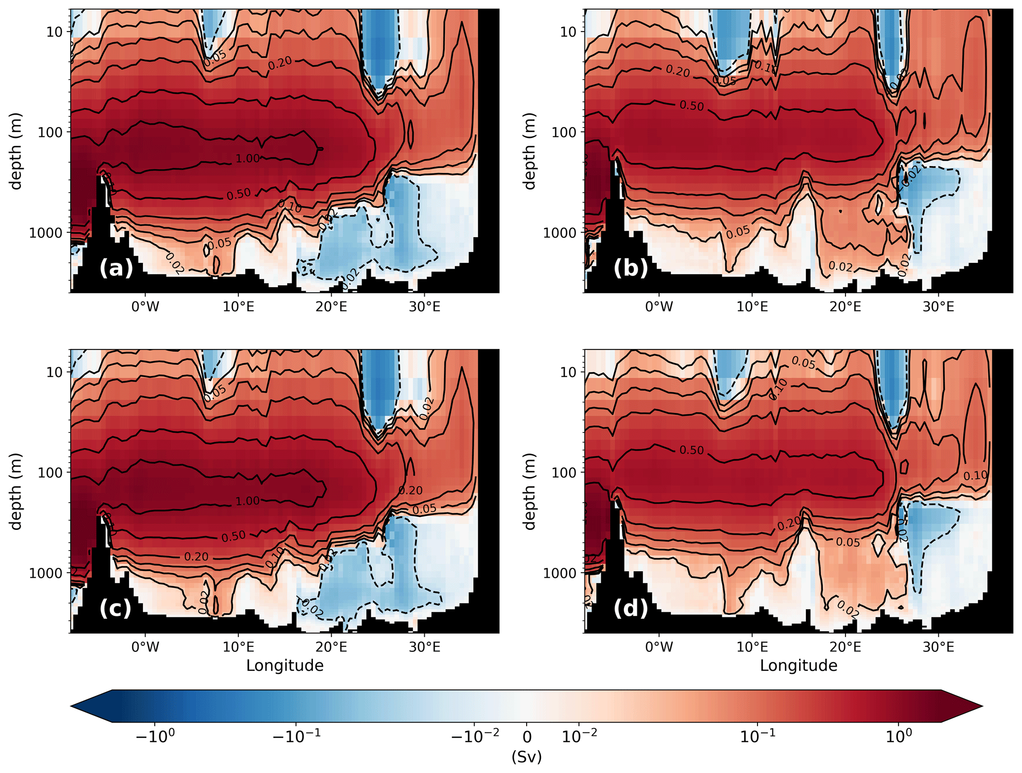
Figure 4 Mean zonal stream function (Sv) of GLAC-1D (a, b) and ICE-6G (c, d) for the PI (a, c) and the LGM (b, d). Contour lines are given as a dashed line for (−0.02) and as solid lines for (0.02), (0.05), (0.1), (0.2), (0.5), and (1.0). Please note the logarithmic depth scale and the logarithmic colour scale.

All simulated biogeochemical patterns of the PI reflect the typical west–east gradient. Higher nutrient surface concentrations and a correspondingly higher net primary production (NPP) are found in the western basin, while more oligotrophic conditions are simulated for the eastern basin, with the exception of the region downstream of the Nile river mouth (Fig. 5a). Note that our simulation is based on conditions prior the construction of the Aswan High Dam in 1964. High NPP is found in the Alboran Sea and in the modified Atlantic water flowing along the coast of Africa into the Ionian Sea. A local high is also found in the GOL, fuelled by nutrient supply due to deep winter mixed layers. The oligotrophic eastern Levantine has the lowest net primary production, about half that of the GOL, which is in line with observational estimates. Compared to satellite-derived estimates from Uitz et al. (2012), our simulated NPP is rather on the low side but fits well within the range of other modelling studies (Table A1). However, the absolute value of the NPP is not so relevant for our study. The amount of exported nutrients from the surface layers below the euphotic zone is more important as it shapes the nutrient profile.

Basin-wide mean phosphate profiles below 100 m fit well to observations (Fig. 2c and g) with sightly lower concentrations below 1000 m. Simulated mean surface concentrations in the euphotic zone (upper 100 m) are rather low compared to MEDATLAS in all basins. However, revisiting the climatological mean concentrations of the upper 150 m for 1981–2017 by Belgacem et al. (2021) showed that the climatology of MEDATLAS has the tendency to overestimate the nutrient concentration, e.g. in the Gulf of Lion. Oxygen concentrations below the euphotic zone are slightly higher than the climatology (20–40 mmol O₂ m⁻³). Part of this discrepancy could be related to the missing anthropogenic nutrient input (riverine and atmospheric) which increased dramatically after 1950 for N and P (Krom et al., 2014). Other nutrient sources like the simulated N fixation show also higher values in the western basin than in the eastern basin, in line with observations (Krom et al., 2014), but they play a negligible role overall (not shown).

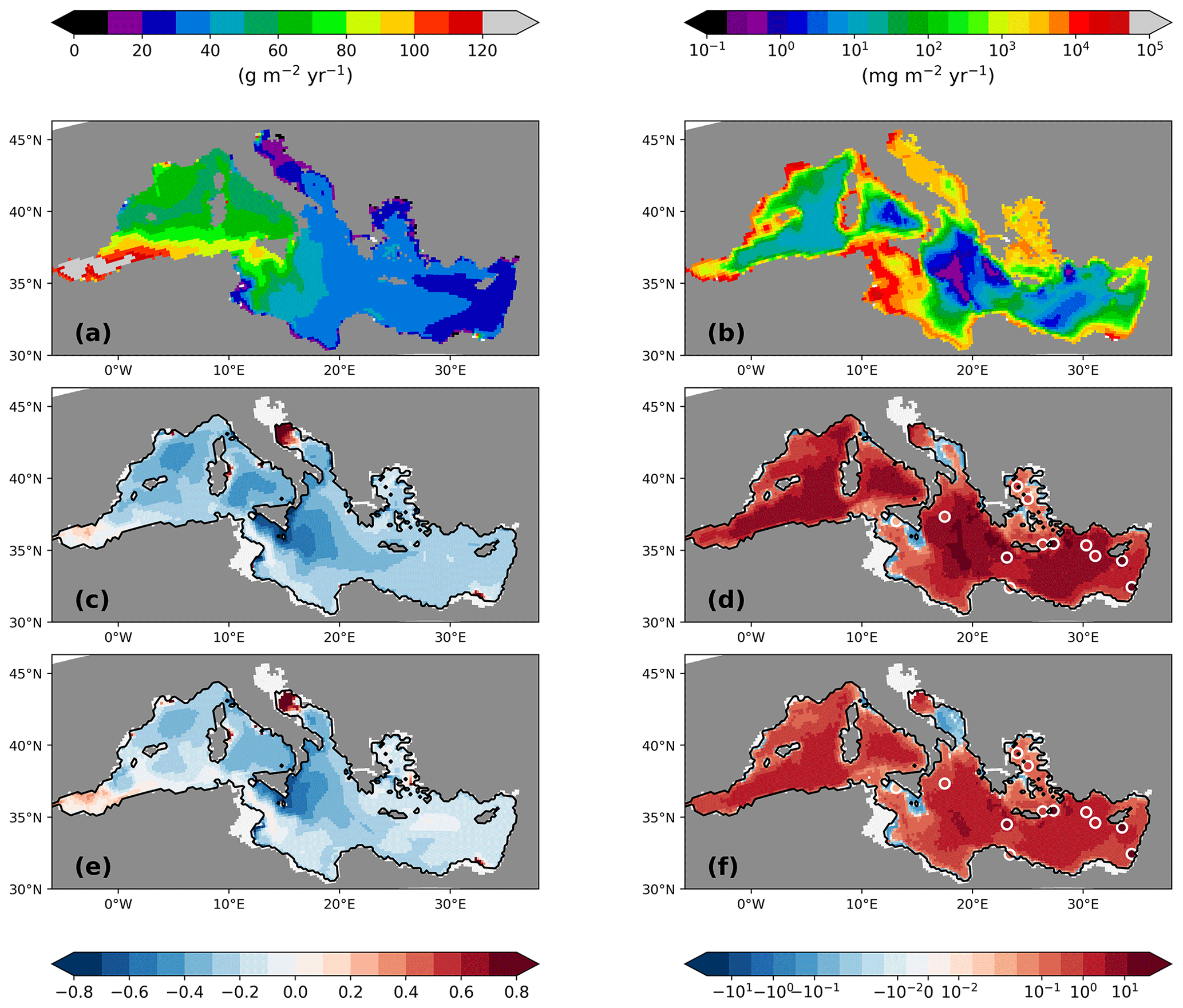
Figure 5 Vertically integrated NPP (a; g C m⁻² yr⁻¹) and settling flux of organic material into the sediment (b; mg C m⁻² yr⁻¹) for the PI of GLAC-1D and the relative changes between the LGM and the corresponding PI for NPP of GLAC-1D (c) and ICE-6G (e) and for the sedimentation rates of GLAC-1D (d) and ICE-6G (f). Note the logarithmic colour scales in panels (b), (d), and (f). The black contour line indicates the LGM coastline. Overlaid circles in panels (d) and (f) are relative changes in benthic foraminiferal numbers between LGM and PI (Schmiedl et al., 2010, 2023).

Biogeochemical settling processes do not only shape the vertical profiles but also leave their imprint in the sediment. The spatial pattern of the sedimentation rate of organic material primarily reflects the local ocean depth (Fig. 5b). In the deep basins of the eastern MedSea, the sedimentation flux is less than 1 mg C m⁻² yr⁻¹ compared to a vertically integrated net primary production of approximately 40 g C m⁻² yr⁻¹. Only the shallower shelf areas receive higher organic matter fluxes, as well as a higher deposition fluxes of opal shells, which are clearly visible in the weight percentage contributions of detritus and opal in the upper 6 mm of the sediment column (first two layers) (Fig. 6). Note that the remaining percentage part consists primarily of calcium carbonate (CaCO₃) and terrigenous material (Fig. A3). The largest weight percentage contribution of 40 %–70 % provides CaCO₃, which displays a pattern very similar to that of NPP. Similar carbonate contents have been documented in sediment cores from different Mediterranean basins (Aksu et al., 1995; Hoogakker et al., 2004; Hamann et al., 2008). The simulated CaCO₃ pattern with lower values in the northeastern Levantine and higher values in the Ionian Sea towards the Strait of Sicily agrees qualitatively well with the data compilation of Venkatarathnam and Ryan (1971). Supersaturation of the entire water column in the MedSea with respect to calcite prevents the dissolution of CaCO₃ shells (Béjard et al., 2023) and maps the pattern of planktic calcite shell production on the seabed. For detritus and opal shells, remineralisation and dissolution reshape the particle settling fluxes which decrease with increasing water depth. The sediment in all deep basins consists of less than 0.01 % detritus or opal shells. Only in the shallower shelf areas are 1 %–2 % weight percent of the sediment detritus and 2 %–10 % opal shells. Given the simplicity of the sediment module and the coarse horizontal resolution of the medHAMOCC, these results fit very well with the few available core-top data for the present day (Pedrosa-Pàmies et al., 2015). Sediment erosion, i.e. resuspension of all solid sediment material with the exception of sand, occurs primarily in the Strait of Gibraltar, the Strait of Sicily, and near the shore on the Tunisian shelf. However, the simulated resuspension is probably underestimated due to the reduced variability in monthly mean forcing data, but observational data are missing, preventing an evaluation of our model results.

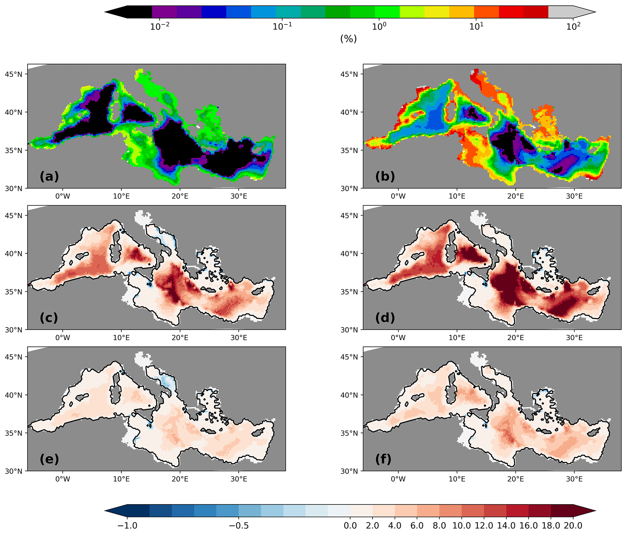
Figure 6 Weight percentage sediment contribution in the upper 6 mm of the sediment column of detritus (a) and opal (b) for the PI of GLAC-1D (in %). Relative changes between the LGM and the corresponding PI are given for detritus (c, e) and opal (d, f) for GLAC-1D (c, d) and ICE-6G (e, f). Note the logarithmic colour scale for panels (a) and (b) above the figure and the nonlinear colour scale for panels (c)–(f) below the figure.

4 Changes in the patterns of the Last Glacial Maximum

4.1 Changes in the physical environment

The sea surface temperatures of the LGM in both simulations are generally about 4–8 K lower than for the PI (Fig. 7a and c), which is in line with palaeo-temperature estimates (Hayes et al., 2005; Kuhlemann et al., 2008). The comparison to sea surface temperature (SST) reconstructions from planktic foraminiferal assemblages (Hayes et al., 2005) shows that model biases are within the range of results for different reconstruction methods (Figs. 8 and 9). Out of the parent simulations, GLAC-1D has a weaker Atlantic overturning circulation and a relatively colder climate over the North Atlantic than ICE-6G (Kapsch et al., 2022), which is reflected in the larger SST anomaly (and larger deviation from the reconstructions; Fig. 9) throughout the entire MedSea.

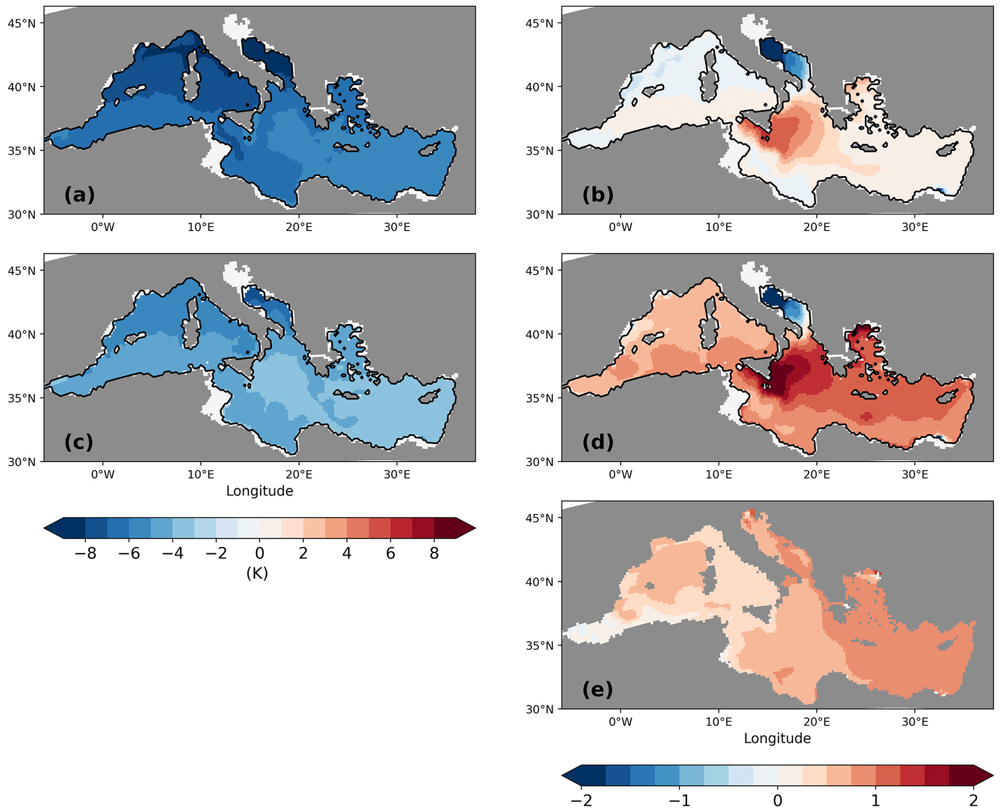
Figure 7 Anomalies of sea surface temperature (K) (a, c) and sea surface salinity (b, d) between LGM and PI for GLAC-1D (a, b) and ICE-6G (c, d). Panel (e) shows the anomaly of sea surface salinity between PI-Straits and PI of GLAC-1D. The anomaly of sea surface temperature between PI-Straits and PI of GLAC-1D is small (not shown).

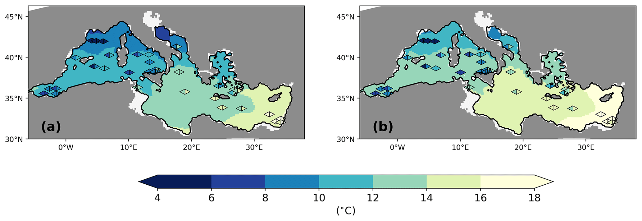
Figure 8 Annual mean sea surface temperature (°C) at the LGM for GLAC-1D (a) and ICE-6G (b). Overlaid data from Hayes et al. (2005) are estimates from two different methods, namely the artificial neural network (left part of the rhombus) and the revised analogue method (right part of the rhombus). See Hayes et al. (2005) for more details.

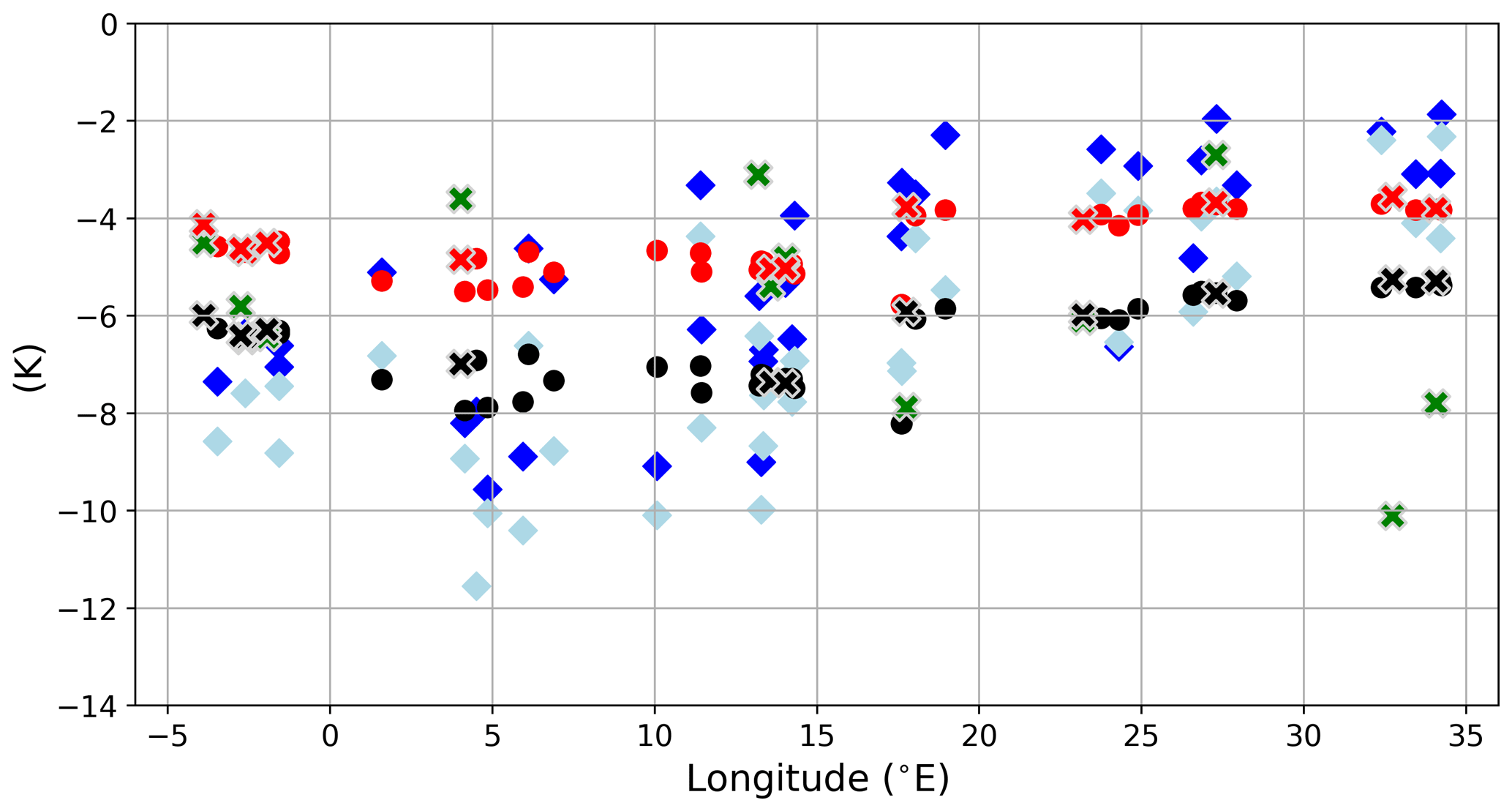
Figure 9 Annual mean SST differences between LGM and PI for GLAC-1D (black circles) and ICE-6G (red circles) against the longitude. Overlaid are the same SST data, as in Fig. 8, using an artificial neural network (blue diamond) or the revised analogue method (light blue diamond) but shown here as the deviation from modern SST (World Ocean Atlas; Locarnini et al., 2018). In addition, SST change estimates based on alkenones from Lee (2004) with updates from the PANGAEA database (Herbert et al., 2018; Rodrigo-Gämiz et al., 2014; Castañeda et al., 2010) are given (green crosses) with the corresponding SST difference for GLAC-1D (black crosses) and ICE-6G (red crosses). Units are in kelvin.

For the Gulf of Lion, the annual SST of the LGM is much higher in both simulations than in the reconstruction, creating a larger deviation in the proxy data compared to the eastern basin (Figs. 8 and 9). As the coarse-resolution atmospheric parent models are missing the permanent ice cover over the Alps, the transport of cold air towards the gulf is potentially underrepresented in the summer season and causes this bias (Fig. A4).

We also find an intensification of the SST gradient between the eastern and western basin during the LGM, as proposed by Hayes et al. (2005). Annual mean temperature differences between GOL and LEV rise from 2 K to about 4.5 K (Fig. 2).

Sea surface salinity (SSS) changes show a very similar spatial pattern for both simulations with a higher SSS change in the eastern basin. GLAC-1D has a lower SSS increase than ICE-6G (Fig. 7b and d). This is partly due to a negative SSS anomaly at the Strait of Gibraltar entrance (Fig. 7d). The water mass boundary of the subpolar gyre in the North Atlantic of the parent simulation of GLAC-1D shifts further to the south compared to ICE-6G during the LGM. Thus, in a colder GLAC-1D climate, less saline subpolar water enters the Gulf of Cádiz and imprints on the SSS anomaly of the MedSea. The most pronounced increase in SSS is found in the Ionian Sea, which is attributable to changes in the circulation linked to the freshening of the Adriatic Sea and the consequential strong reduction in local deep-water formation (see the discussion on pycnocline changes below). The modelling study by Mikolajewicz (2011) demonstrated a similar shift in the area of deep-water formation from the Adriatic Sea to the Ionian Sea that was also accompanied by the largest SSS increase from the present day to LGM. In contrast to Mikolajewicz (2011), the Adriatic Sea keeps a weak anti-estuarine circulation during the LGM in our simulations.

SSS changes between the LGM and present day based on δ¹⁸O reconstructions from planktic foraminifera were estimated to +1.2 (+2.7) in the western (eastern) basin (Thunell and Williams, 1989), which is about 1–1.5 higher than our results. However, these estimates come with an unclear uncertainty. The underlying method combines global δ¹⁸O changes due to ice sheet growth (1.2 ‰ with a potential error of approx. 30 %; Schrag et al., 2002), LGM temperature estimates from alkenone ratios (uncertainty ±1.3 °C⁻¹; Sijinkumar et al., 2016), and a global δ¹⁸O salinity slope regression (0.41 ‰ psu⁻¹, Thunell and Williams, 1989; 0.25 ‰ psu⁻¹–0.45 ‰ psu⁻¹, Emeis et al., 2000). Sijinkumar et al. (2016) performed an error propagation for reconstructed LGM salinities in the Bay of Bengal and calculated an error range of 1.8–2.6 for salinity change estimates of 0.9–3.5 between the LGM and the modern ocean. Given these large uncertainties in the SSS reconstruction, we cannot assess our model results based on these literature estimates. Our simulated SSS changes are at least consistent with the applied forcing. Besides the changing salinity in the Gulf of Cádiz, which is determined by the parent simulation, we find, e.g., that the spatial SSS difference between the Levantine and the Gulf of Lion increases by 0.3 from the PI to the LGM in GLAC-1D (0.5 for ICE-6G) (Fig. 2). This is attributable to a longer residence time of the water within the basins due to a reduced zonal overturning circulation (ZOC), which also means that the surface water is exposed to net evaporative fluxes for a longer time.

The ZOC of both experiments shows that the strong, deep-reaching anti-estuarine circulation (maximal transport of 1.2 Sv; vertical extension to 600–800 m) in the PI is reduced to ∼0.6 Sv and only reaches 400 m depth in the LGM (Fig. 4). The reduction in the ZOC is linked to the change in the outflow at the Strait of Gibraltar due to the lower sill depth (Fig. 3; Table 1), changed freshwater budget (Table 2), and a concurrent increase in the salinity gradient between surface and intermediate layers (0.17–0.265 between 466 m and surface; Fig. 2). The magnitude of the simulated ZOC reduction fits well to the previous estimates of 40 %–65 % from modelling studies (Myers et al., 1998; Mikolajewicz, 2011) and theoretical considerations (Rohling, 1991, and refs within). About two-thirds of the ZOC reduction can be attributed to a reduced cross-sectional area in the Strait of Gibraltar, as demonstrated by the sensitivity study PI-Straits (Fig. 3 and its zonal stream function in the Appendix; Fig. A1).

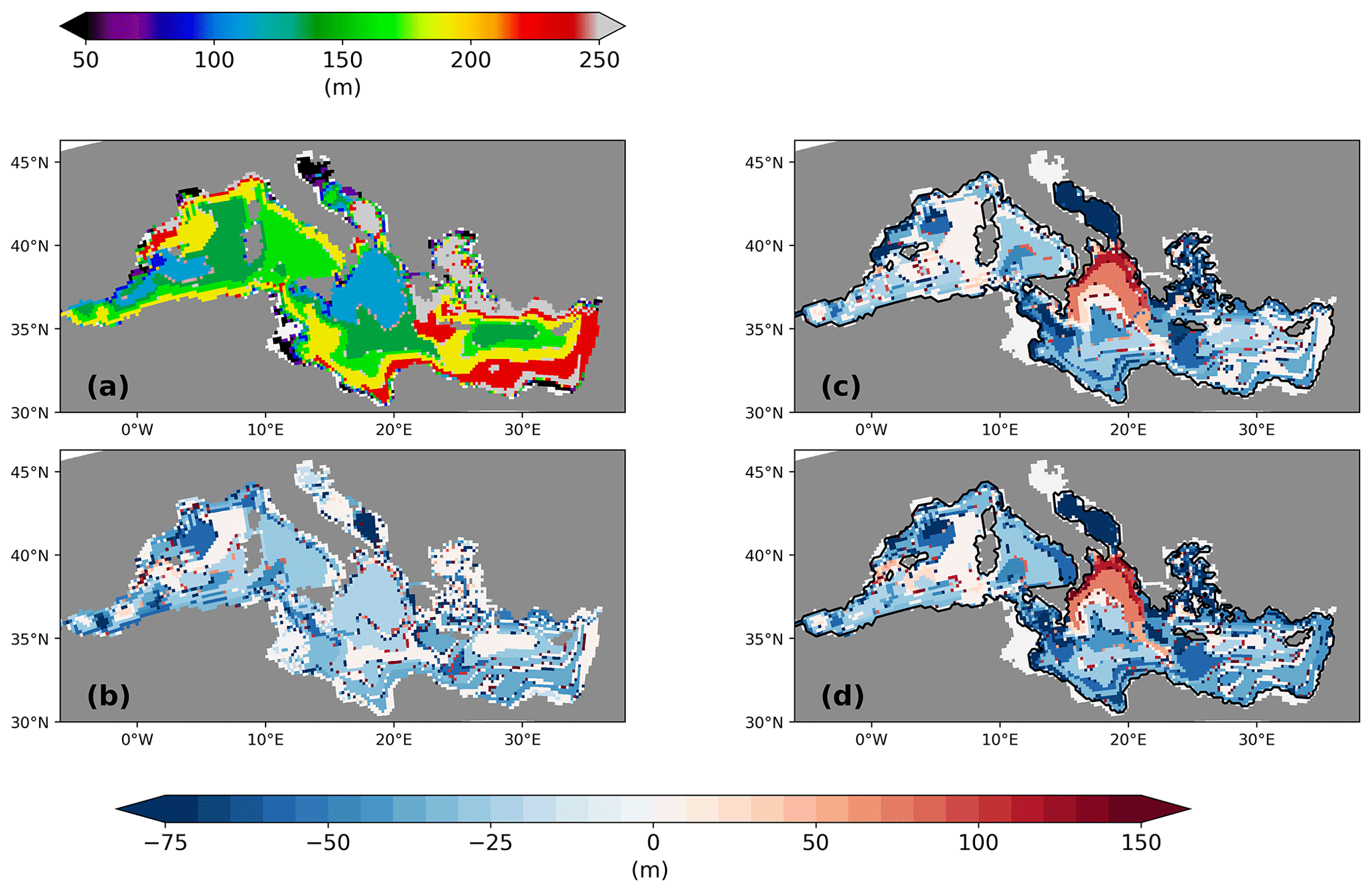
Figure 10 Depth of pycnocline in February for PI of GLAC-1D (a) and the pycnocline depth change between LGM and PI for GLAC-1D (c) and ICE-6G (d). Panel (b) gives the pycnocline depth change between PI-Straits and the PI of GLAC-1D. Units are in metres.

To gain more insight into the combined effects of the LGM changes in SST, SSS, and ZOC on the circulation, we investigate the depth change in the pycnocline in February when a shallower winter pycnocline depth could allow a higher nutrient supply to the productive surface layers, as postulated by Rohling (1991). The pycnocline depth in February for the PI of both experiments is very similar, as a consequence of the similarity of the parent simulations for PI. Figure 10 shows, therefore, only the result of the PI for GLAC-1D. For the LGM, we see a shallowing of the pycnocline by 20–60 m for most areas of the MedSea in both simulations. This corresponds to a relative shallowing to 65 %–85 % of the PI value, which is similar to the estimate of Rohling (1991) and is in line with his theoretical approach. In regions of deep-water formation in the PI (i.e. the Gulf of Lion and the Adriatic Sea; Fig. A2), the shallowing is more pronounced (>60 m) due to an increased water column stability. Only the northern Ionian Sea shows a strong deepening of the pycnocline for the LGM, which is linked to the lack of deep-water formation in the Adriatic Sea (Fig. A2). During the PI, dense water is formed in the Adriatic Sea, flows across the Otranto sill, supplies the deep and intermediate water of the northern Ionian Sea, and, thus, lifts up the density isosurfaces (Liu et al., 2021). This deep-water formation during the PI leaves its imprint on the water masses of the northern Ionian Sea where colder, less saltier, and “younger” water mass properties are found at intermediate water depths in the west of the Ionian basin compared to the east (not shown). At the LGM, water mass properties are very similar across the entire northern Ionian basin, and thus, we find a deepening of the pycnocline primarily along the eastern side of the Ionian basin. In the sensitivity study PI-Straits, the deep-water formation in the Adriatic Sea is slightly reduced but still active (Fig. A2c), and hence, we do not find a corresponding pattern in the pycnocline depth change (Fig. 10). The similarity of the spatial pattern in PI-Straits compared to the LGM simulations underlines that shallower sill depths alone are the largest contributor to the pycnocline anomaly for most areas of the MedSea. The reduced ZOC (Fig. 3) and the consequently longer water residence time within the basins of the MedSea increases the SSS (Fig. 7) and intensifies the water column stratification in all experiments with LGM sill depth (Fig. 2b and f).

4.2 Changes in the biogeochemical distributions in the water column

Following the argument by Rohling (1991), who postulated that a shallower pycnocline provides more nutrients to the production zone and enlarges the NPP, we might expect, according to Fig. 10, an increase in the surface phosphate concentration and NPP. In contrast, the simulated surface phosphate concentration at the LGM decreases remarkably by 20 %–60 % compared to its PI value (Fig. 11b and d). Consequently, the vertical integrated net primary production resembles this pattern change (Fig. 5c and e). The largest changes in surface phosphate and NPP are located in deep-water formation areas and the western Ionian Sea. Suppressed or shallower deep-water formation hampers the supply of phosphate (PO₄) to surface layers. Relative increases in surface phosphate are found only in the Alboran Sea and in the vicinity of rivers. The increased river runoff during the LGM (Table 2) also transports more nutrients (phosphate, nitrate, and silicate) to the MedSea, according to our parameterisation which is based on a basin-wide fixed river nutrient concentration times river discharge. The relative increase in NPP in the vicinity of the Nile river underlines the change in the runoff (Fig. 5c and d). In the northern Adriatic Sea, we see a relocation of the productive area. Bathymetry changes due to the low sea level stand move the coastline and, thus, the river estuaries towards the south. Note that we find a similar overall relative decrease in surface PO₄ for PI-Straits, only missing the extreme changes in deep-water formation areas and the northern Adriatic Sea (Fig. 11c).

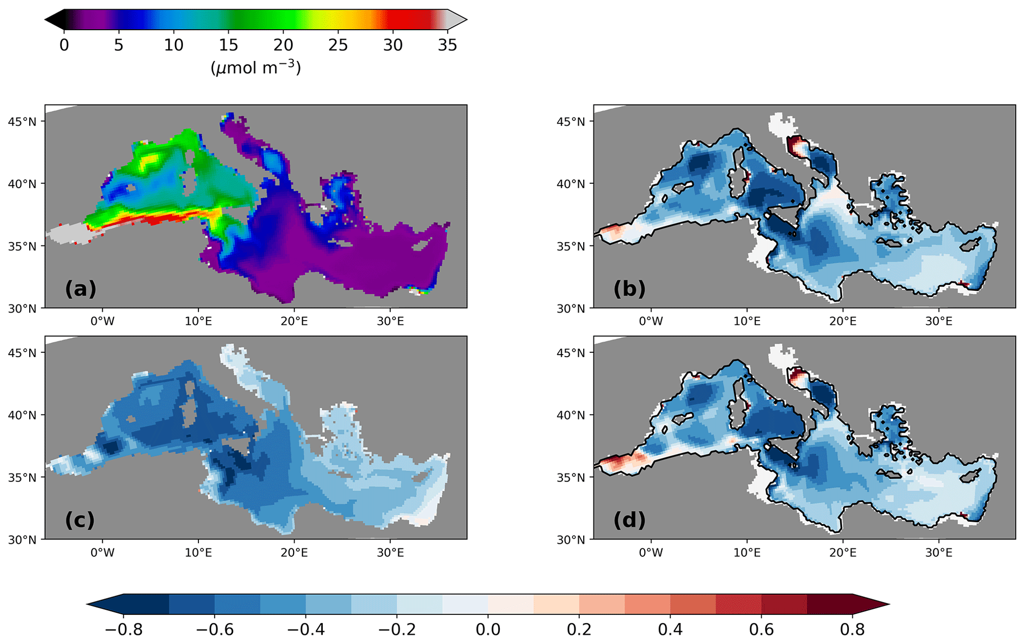
Figure 11 Surface phosphate concentration (µmol P m⁻³) for the PI of GLAC-1D (a; see the colour scale above panel a) and its relative concentration change between the LGM and the PI for GLAC-1D (b) and for ICE-6G (d). Panel(c) shows the relative concentration change between PI-Straits and the PI of GLAC-1D.

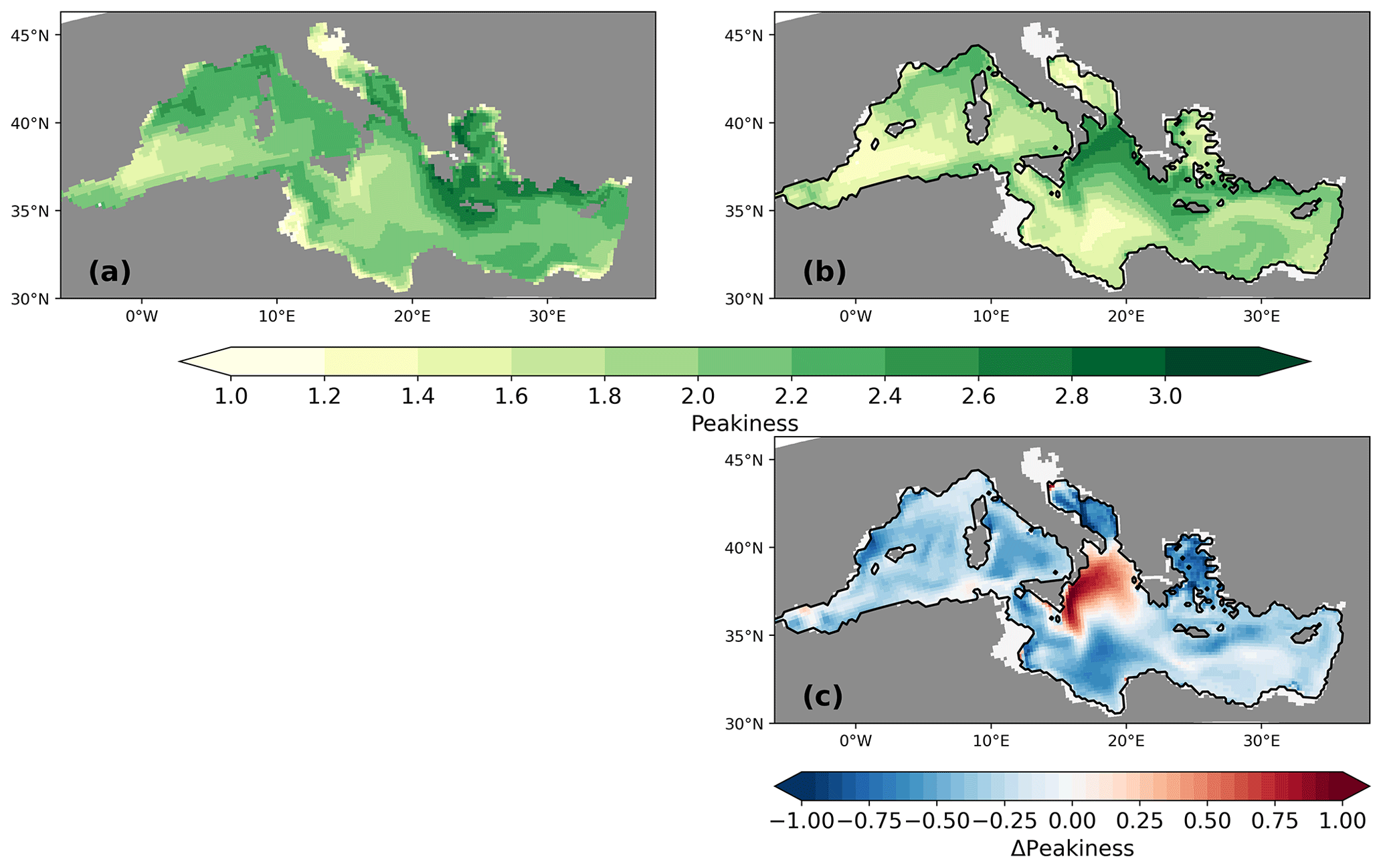
Figure 12 Peakiness P for the PI (a) and the LGM (b) of GLAC-1D and the difference between LGM and PI of P. See the text for a definition of peakiness.

Besides an overall decrease in the annual mean NPP, we also find a flattening of the seasonality of the production. To illustrate the changes in the NPP seasonality, we define the peakiness of the seasonal NPP with

$$\begin{array}{}\text{(1)}& P={\displaystyle \frac{\mathrm{12}{\mathrm{NPP}}_{\max }}{\sum {\mathrm{NPP}}_{\mathrm{ann}}}},\end{array}$$

where NPP_max is the annual maximum of the monthly mean NPP (we use a running mean of 2 months to ensure that we find a correct maximum within our monthly mean data), and ∑NPP_ann is the total annual NPP. In case of the same NPP for each month, P would be exactly 1. For P=3, 50 % of the annual NPP is confined to 2 adjacent months. For the theoretical case of P=6, 100 % of the annual NPP would occur in 2 adjacent months. The peakiness is, thus, a simple measure to characterise the “blooming areas” and “non-blooming areas” independent of the annual mean NPP (see a similar approach by D'Ortenzio and Ribera d'Alcalà, 2009). For the PI, the peakiness is close to 3 in the Aegean and the northern Levantine and well above 2.2 for the Gulf of Lion and large parts of the Levantine, indicating a well-developed seasonal peak in the production, primarily in spring, and a lower production throughout the rest of the year (Fig. 12). Coastal areas, especially in the vicinity of rivers, show a more uniform production seasonality (P close to 1). This pattern for the PI resembles the findings of D'Ortenzio and Ribera d'Alcalà (2009), who characterised the seasonal cycle of surface biomass for different areas of the MedSea based on satellite data. For the LGM, the seasonality of the NPP flattens throughout the entire MedSea. The northern Ionian Sea is the only exception for which we find a shift towards blooming conditions. The pattern change in the peakiness resembles the changes in the pycnocline (Fig. 10), which might explain the changes in the nutrient supply throughout the year.

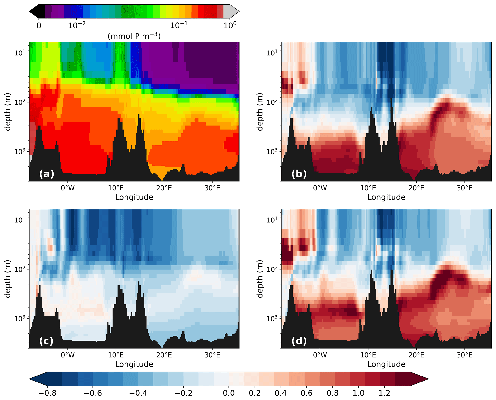
Figure 13 Phosphate concentration (mmol P m⁻³) along the west–east transect (for the location, see Fig. 1) of the PI of GLAC-1D (a) and the relative concentration change between the LGM and the corresponding PI of GLAC-1D (b) and ICE-6G (d) and between PI-Straits and the PI of GLAC-1D (c). Note the logarithmic colour scale in panel (a) and the logarithmic depth scale in all panels.

To understand the fate of the surface nutrients, we first look at the vertical PO₄ distribution. As already visible in the concentration profiles for the GOL and the LEV (Fig. 2), we see a strong accumulation of PO₄ below 100 m during the LGM. The west–east cross section through the MedSea displays sharp vertical gradients around 100 m with relative changes of more than 100 % in both basins and both LGM simulations (Fig. 13). In PI-Straits, an accumulation of PO₄ at depth is missing, and we instead find a nutrient depletion over the entire MedSea. The shallower sill depths in the LGM and PI-Straits lead not only to a more sluggish overturning circulation (Fig. 4) but also to a shift in the centre of the maximum zonal transport to a shallower depth. This causes a very effective lateral export of nutrients and organic material at an intermediate depth from the eastern to the western basin and out of the MedSea and, thus, leads to the depletion of nutrients in PI-Straits. In the LGM simulations, the same process is active but is overcompensated by the effect of an additional change in the remineralisation rate of organic material. The remineralisation rate depends primarily on temperature and oxygen availability. Any potential restrictions by oxygen are negligible in the well-ventilated water of the MedSea during the PI and the LGM (Figs. 2 and A5). Temperatures at the LGM are significantly lower by −8 to −4 K than in the PI (Fig. 2), causing remineralisation rates to drop to 51 %–64 % of the PI values, respectively. In combination with gravitational sinking, more detritus reach intermediate and deep layers and potentially enter the sediment in the LGM simulations. The transfer efficiency of detritus T_eff (Weber et al., 2016) which relates the detritus sinking flux at 1000 m to that of 100 m illustrates the effect of the remineralisation rate (Fig. 14).

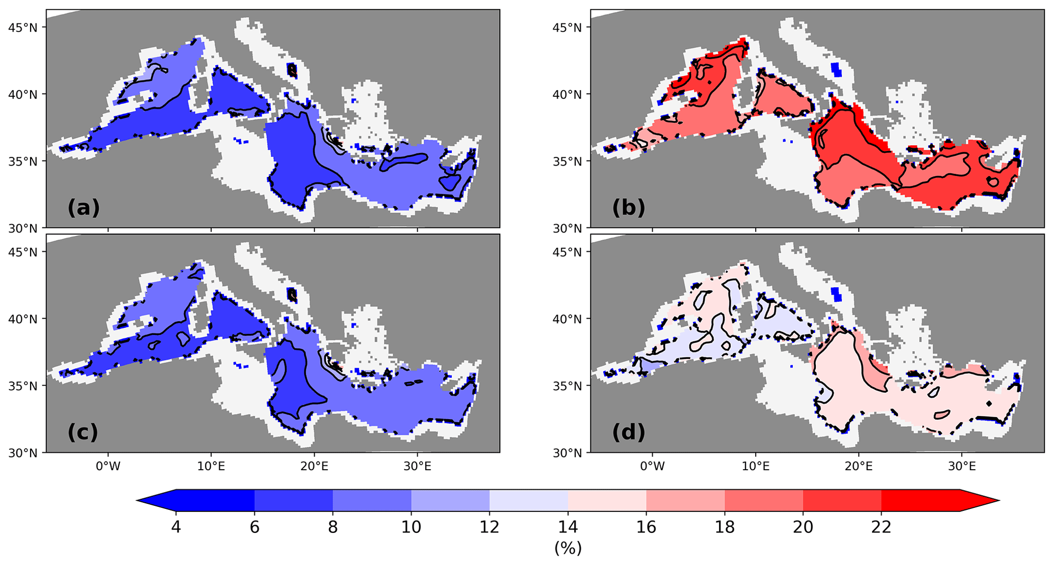
Figure 14 Transfer efficiency of detritus calculated as ratio of the detritus flux at 1000 to 100 m on a percentage basis (%) for the PI of GLAC-1D (a) and for the LGM of GLAC-1D (b) and ICE-6G (d). Panel (c) gives the transfer efficiency for PI-Straits.

In the PI, less than 10 % of the detritus export flux at 100 m reaches the 1000 m depth level. This is also true for PI-Straits which has a nearly identical vertical temperature distribution as the corresponding PI simulation (differences smaller than ±0.5 K between PI-Straits and PI of GLAC-1D; not shown). In contrast, T_eff increases to 14 %–28 % in both LGM simulations. Higher T_eff in the LGM of GLAC-1D than in ICE-6G is attributable to the overall colder conditions in this simulation (Figs. 2 and 7). To further illustrate the combined effects of shallower sill depths and colder temperatures on the nutrient distribution, we present, as an example, the dynamical conditions in the Strait of Sicily for GLAC-1D (Fig. 15). The mean transport of total phosphate (i.e. the sum of dissolved and organically bound phosphate) across the strait is southward in the upper 137 m for the PI, with a corresponding northward return flow below. With the shallower strait depths for GLAC-1D-LGM and PI-Straits, the interbasin exchange fluxes are, as expected, reduced, and the neutral position between the baroclinic flow components shifts to 111 and 97 m, respectively. Below this depth, both simulations show a more effective export of total phosphate from the eastern basin compared to GLAC-1D-PI. In combination with a reduced inflow of total phosphate into the eastern basin, this leads to the simulated nutrient depletion in the upper 200 m of the water column (as seen in Fig. 13). The warmer temperatures in PI-Straits than in the GLAC-1D-LGM allow a higher biological production despite the similar near-surface phosphate concentration indicated by the slightly higher organically bound phosphate concentration in the upper ocean (Fig. A6b). However, the temperature effect on remineralisation manifests in a more rapid decay of detritus and a higher phosphate concentration between 100–200 m in PI-Straits compared to the LGM simulation of GLAC-1D (Fig. A6a), eventually leading to the even larger nutrient depletion of the upper ocean.

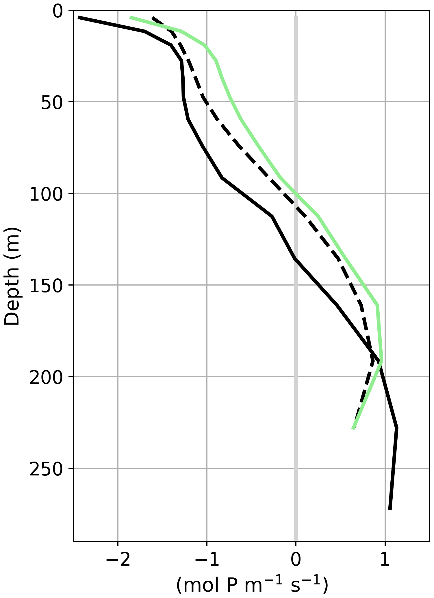
Figure 15 Vertical depth profile of the meridional transport of the sum of the dissolved and organically bound phosphate (mol P m⁻¹ s⁻¹) over the Strait of Sicily for the PI (solid black line) and the LGM (dashed black line) of GLAC-1D and PI-Straits (solid green line). Positive values indicate northward transport, i.e. from the eastern to the western basin of the MedSea.

In brief, the impact of shallower sill depths is primarily a shallowing of the overturning circulation which leads to the more effective zonal export of nutrients from intermediate ocean depths. As seen for PI-Straits, the phosphate inventory of the entire MedSea consequently decreases even under present-day climate conditions. Furthermore, a potential increase in net primary production due to a shallower pycnocline, as proposed by Rohling (1991), is outweighed by this efficient drainage of nutrient from the MedSea. For the colder LGM conditions, we find a comparable decrease in surface PO₄ concentrations (Fig. 5) and NPP (Fig. 13), but the temperature-induced lowering of remineralisation rates leads to a higher T_eff and a phosphate accumulation at greater depths. It is important to emphasise that a higher T_eff during the LGM masks the signal of the lower surface net primary production and leaves its imprint in the sediment. The implications will be discussed in Sect. 4.3.

4.3 Changes in the sediment composition for the LGM

As previously mentioned, changes in the remineralisation rate also modify the deposition flux to the sediment. Relative changes in the settling flux rate, especially in the deep Ionian Sea, are 5–10 times higher than during the PI, while NPP decreases to −0.4 to −0.6 in the same area (Fig. 5). Note that increased deposition fluxes increase the abundance of benthic foramifera in the real world, which is observed for several sediment cores from the eastern basin with a mean relative change in the benthic foraminiferal number of about 7 (range of 0.1 to 30.2; Schmiedl et al., 2010, 2023, and references therein). Hence, our simulated changes in organic matter deposition agree, to the first order, with observed indicators. Figure 6 displays the changes in weight percentage sediment composition between the LGM and the PI. Both LGM simulations show an increased fraction of detritus and opal in the upper 6 mm of the sediment column (first two model layers of the simulated sediment column) with at least a doubling of the local contribution of both components almost over the entire MedSea. Changes in the deep basins are more pronounced due to the higher transfer efficiency at the LGM (factor of 10). Again, the even higher transfer efficiency due to colder temperatures of GLAC-1D is evident from the larger fractional change in detritus and opal. The calcite fraction correspondingly decreases throughout the MedSea, with the largest changes in the Ionian Sea and the Adriatic Sea (<0.5) and more moderate changes in the Alboran Sea (Fig. A3). Sediment core data confirm 20 %–50 % lower-than-modern carbonate contents during the LGM for different areas of the Mediterranean Sea (Aksu et al., 1995; Hoogakker et al., 2004). Please note that in our simulation a large part of the weight percentage change in calcite is related to the higher dust deposition during the LGM, especially in the northern part of the MedSea (Fig. A3; Albani et al., 2016).

Higher accumulation of organic carbon during the LGM compared to the PI is supported by an increased abundance of benthic foraminiferal tests which develops under the elevated food supply of detritus (Schmiedl et al., 2010, and references therein). Hence, our simulated sediment changes are in good agreement with sediment proxies. Moreover, it has to be emphasised that these elevated sedimentary fluxes occur under a simulated lower NPP. Thus, our results link the supposedly contradictory statements of a higher NPP during the LGM, as inferred from benthic proxy data (Schmiedl et al., 2010), and a lower NPP, as derived from the absence of small placoliths, namely Coccolithophoridae, used as a classical indicator of high nutrient availability (Ausín et al., 2015).

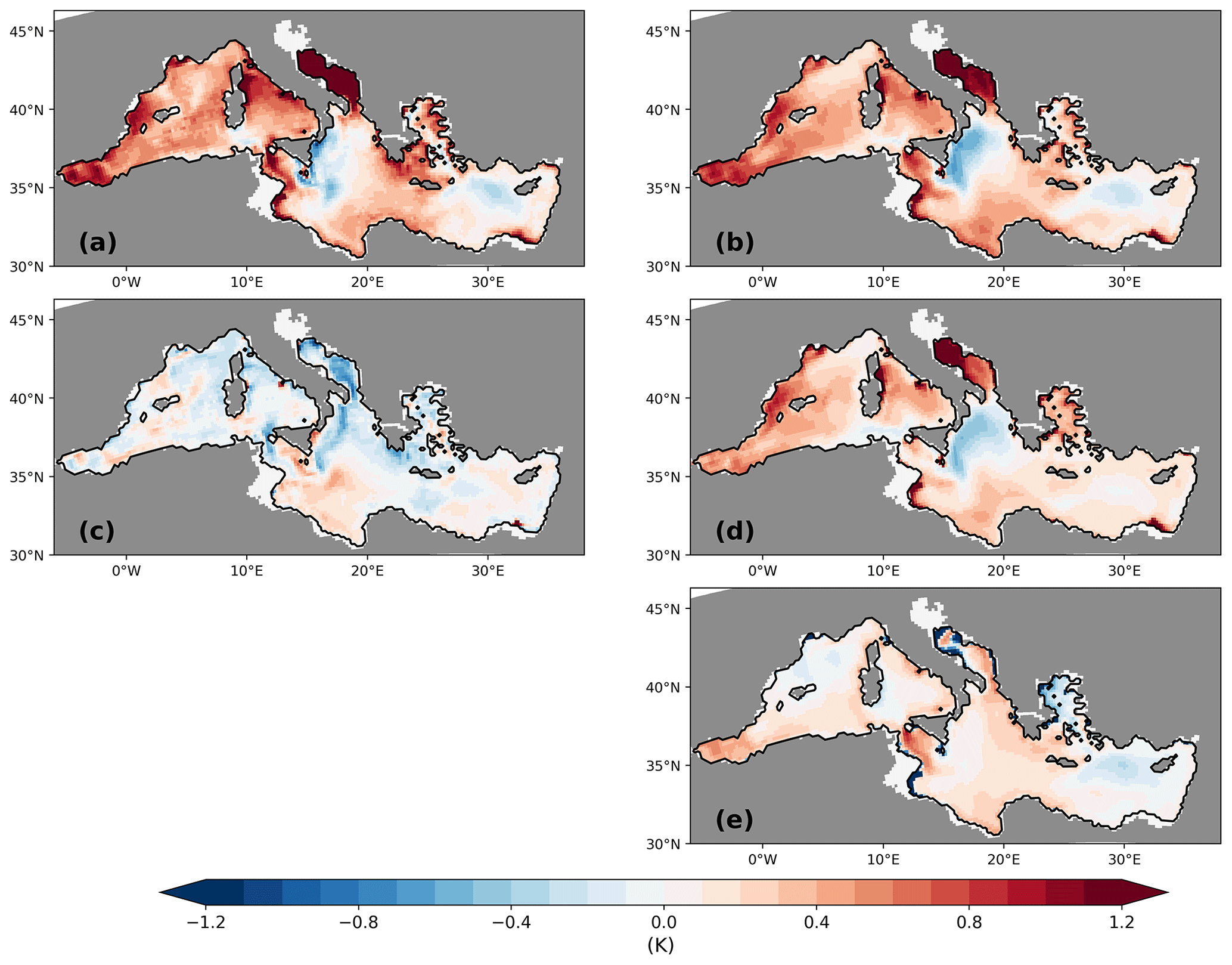
Figure 16 Difference between ΔT_org and ΔT₃₂ (a). Note that both anomalies are negative; thus, positive values in panel (a) indicate a larger absolute ΔT₃₂. Also shown is the difference between ΔPWT and ΔT₃₂ (b) and the difference between ΔPWT and ΔT_org (c). Panel (d) shows ΔPWT_NPP, the NPP-related contribution to ΔPWT, and panel (e) displays ΔPWT_T−ΔT₃₂, the temperature-related contribution. All units are in kelvin. See the text for definitions.

4.4 Assessment of the biological production temperature T_org

The use of the alkenone unsaturation ratio ${\mathrm{U}}_{\mathrm{37}}^{{\mathrm{K}}^{\prime }}$ to estimate the annual mean sea surface temperature is a widely applied palaeoceanographic tool (Müller et al., 1998; Conte et al., 2006). Potential seasonal biases which arise from the marked seasonality in the abundance of primary producers, and the link between primary production and surface ocean temperatures, have been a debatable issue, but for most of the ocean regions, Rosell-Melé and Prahl (2013) concluded that “the integrated sedimentation patterns for ${\mathrm{U}}_{\mathrm{37}}^{{\mathrm{K}}^{\prime }}$ measured in sediment trap time series provide a measure of annual mean SST” and that a seasonal pattern is not apparent in a temperature reconstruction with ${\mathrm{U}}_{\mathrm{37}}^{{\mathrm{K}}^{\prime }}$ in a global application. However, all derived relationships for ${\mathrm{U}}_{\mathrm{37}}^{{\mathrm{K}}^{\prime }}$ are based on modern conditions of spatiotemporal surface ocean temperature patterns and present-day variations in biological production. So far, there are no data or methods to assess these relationships for past climate conditions.

Our diagnostic tracer T_org (see Sect. 2) mimics the information which is obtainable from alkenones without the methodological and physiological uncertainties typical of alkenone undersaturation estimates (Conte et al., 2006). Thus, T_org gives us the opportunity to analyse (i) how well it captures the surface ocean temperature change between past and present and (ii) which processes might contribute to the difference in the signals between T_org and temperature. To tackle these questions, we calculate the change in T_org between the LGM and PI of GLAC-1D (ΔT_org) and the corresponding change in the surface ocean temperature for which we use the annual mean temperature of the upper 32 m (ΔT₃₂; i.e. corresponding to the first four layers of our model), where most of the simulated biological production takes place.

Figure 16a shows the difference between ΔT_org and ΔT₃₂. Note that here we only discuss the analysis for GLAC-1D. The corresponding figure for ICE-6G is given in the Appendix for the sake of completeness (Fig. A7). For most parts of the MedSea, the cooling signal that is captured by ΔT_org is smaller than ΔT₃₂, resulting in an absolute positive difference because both anomalies are negative. In the western MedSea, the absolute value of ΔT_org underestimates that of ΔT₃₂ by 0.4–1 K, and even higher differences are found in a selected areas, e.g. the Adriatic Sea and close to the shelf regions in the western Ionian Sea. Our result indicates that T_org does not just simply reflect T₃₂ but that additional processes must shape T_org. This might be the seasonality of the net primary production or processes within the water column, such as the remineralisation of organic matter during settling. The latter was postulated by Conte et al. (2006), who showed that different remineralisation functions alone led to changes in T_org between 0.4–0.9 K in their hypothetical case studies.

To gain insight into the drivers of T_org, we construct a diagnostic production-weighted temperature (PWT) by integrating the product of the monthly mean NPP and the monthly mean temperature over all layers and all months and dividing the result by the vertically integrated annual NPP. The difference between PWT for the LGM and the PI (ΔPWT) reflects changes in the NPP and its temperature recording without any impact from remineralisation or settling processes. We find a strong similarity between the patterns of (ΔPWT–ΔT₃₂) and (ΔT_org–ΔT₃₂), which underlines that changes in the surface conditions are the major drivers of T_org variations (Fig. 16a and b). This becomes even more obvious when we separate the variations in ΔPWT into a part attributed to the variations in the NPP (ΔPWT_NPP) and a part attributed to temperature variations (ΔPWT_T). For ΔPWT_NPP, we calculate the difference between the present-day temperature times the monthly mean NPP of the LGM and the present-day temperature times the monthly mean NPP of the PI. Thus, we get variations based only on the shift in the NPP seasonality, which results in a changed sampling of the monthly mean temperatures. To calculate ΔPWT_T, we use the present-day NPP times LGM temperatures and present-day NPP times PI temperatures. This gives the contribution from the fact that the annual mean LGM cooling signal is not distributed uniformly over the year. In our GLAC-1D simulation, the Levantine shows a stronger cooling signal than the annual average during February to April, while in the Ionian Sea, the temperatures of July to September primarily contribute to the annual mean LGM cooling signal (not shown).

Figure 16d shows that the pattern of ΔPWT_NPP explains most of the signal found in ΔPWT, including the cooling signal in the northern Ionian Sea. Furthermore, ΔPWT_NPP resembles the pattern of the peakiness change (Fig. 12) with a warming signal in regions with decreasing peakiness, and vice versa. This clearly indicates that the NPP-driven part is the major driver of PWT changes. The temperature-related part ΔPWT_T has a minor contribution to ΔPWT (Fig. 16e), but it explains, e.g., the small cooling signal west of Cyprus. As mentioned before, the absolute spring temperature change in the Levantine is stronger than the annual mean LGM cooling signal. Other potential sampling biases, such as vertical shifts in the production or due to sampling over shallower water depth in the LGM, have no impact on ΔPWT (not shown). The contribution from processes within the water column, e.g. remineralisation or lateral advection, are estimated by the difference between ΔPWT and ΔT_org (Fig. 16c). For most of the MedSea, this contribution is rather small, except for regions in which we also find strong changes in the physical ocean, such as the northern Ionian Sea, the Adriatic Sea, or the Strait of Sicily. A similar pattern for ΔPWT–ΔT_org is seen for ICE-6G (Fig. A7c). We cannot disentangle whether the cause of this signal in T_org is related to the lateral advection of organic material from distant production regions or a temperature-induced remineralisation change or the combination of both.

To summarise, we find that the recorded temperature of ΔT_org underestimates the climate signal which is represented by ΔT₃₂. The shift in the seasonality of the NPP between past and present is a main driver of the difference between ΔT_org and ΔT₃₂, as a more uniform seasonal cycle in NPP tends to sample the relatively warmer temperatures of late spring and summer. Despite the simplicity of our artificial temperature tracer T_org, our simulations might point to the methodological problem of using present-day-derived correlations for palaeo-records. Furthermore, local changes in the biogeochemical patterns increase the uncertainty that is intrinsic to the method (Conte et al., 2006).

5 Summary and discussion

We apply a regional physical–biogeochemical ocean model of the Mediterranean Sea to investigate the biogeochemical state during the LGM. The use of a novel set of atmospheric and oceanic boundary conditions derived from palaeo-simulations over 26 000 years with an Earth system model (MPIESM; Kapsch et al., 2022) allows running consistent time slice simulations for the LGM and the PI. To address uncertainties for the LGM, we take forcing data from two MPIESM runs based on different ice sheet reconstructions (Tarasov et al., 2012; Peltier et al., 2015). The computational efficiency of our calculations enables transient model simulations over 2000 years, which minimises model drift and permits us to attribute the simulated changes to physical and biogeochemical variations during the LGM. Our analysis is supported by a sensitivity study with present-day climate and LGM strait bathymetry (PI-Straits) to disentangle topography-driven and climate-induced changes in the biogeochemistry.

Simulated circulation changes for the LGM are primarily caused by sea level low stands which lead to a weakening of the zonal overturning circulation and an intensification of water column stability. Our model results for the PI and the LGM are in line with previous ocean modelling attempts (Myers et al., 1998; Mikolajewicz, 2011; Sevault et al., 2014; Grimm et al., 2015) and theoretical considerations (Rohling et al., 2015). Simulated changes in sea surface temperature fall into the range of estimated surface cooling (Hayes et al., 2005).

The similarly strong response of the biogeochemistry in both LGM simulations indicates the robustness of the signals, such as the nutrient accumulation below 100 m in the western and eastern basin of the MedSea. A quantitative evaluation of our simulated LGM distributions is still challenging. The evaluation of our results on the changes in the biogeochemistry during the LGM is restricted to the comparison to sediment core data because, to our knowledge, there is no other published modelling study for the MedSea on this topic. As deduced from the sediment archives, an observed increase in the diversity and the proportion of infaunal benthic foraminifera supports a glacial increase in the organic matter fluxes to the seafloor (Schmiedl et al., 1998; Kuhnt et al., 2007; Abu-Zied et al., 2008; Schmiedl et al., 2010). Our model simulations confirm a higher detritus deposition, but this emerges from lower surface net primary production. Nutrient availability at the surface is reduced due to the higher water column stability, a more efficient lateral nutrient export at mid-depths out of the MedSea, and a larger transfer efficiency of detritus at 1000 m under the cold LGM climate. A simulated lower production during the LGM is in agreement with the data of the sediment composition which show an absence of small placoliths, with Coccolithophoridae used as classical indicator for high nutrient availability (Ausín et al., 2015). The occurrence of higher depositional fluxes despite lower primary production may clarify the supposed inconsistencies in the interpretation of sediment data.

Our results emphasise the non-linearity of the response of the biogeochemistry to the hydrodynamical changes at low sea level stands. The assumption that the shallowing of the pycnocline inevitably introduces higher net primary production (Rohling, 1991) must be revised, and the interplay of altered lateral transport and reduced biological turnover rates must be considered for the LGM. This is underlined by the findings of the sensitivity experiment PI-Straits. By only reducing the water inflow from the Atlantic due to a shallower sill depth, most of the biogeochemical pattern changes in the upper ocean, which are found for the LGM, are reproduced under the present-day climate. Our findings clearly point to the need for long-term modelling attempts, ideally with a suite of different ocean biogeochemistry models, to gain further insights into the mean state and the temporal variations in the last glacial.

A noteworthy additional outcome of our simulations is provided by the artificial temperature tracer T_org. Changes in temperature of the upper 32 m between LGM and PI are imprinted on the sediment with a spatial heterogeneous pattern. In the western Mediterranean Sea, the T_org signal underestimates the LGM upper-ocean temperature anomaly by about 1 K, while T_org records a stronger cooling of up to 0.5 K for the northern Ionian Sea. Thus, even within our ideal model world where all physiological and methodological uncertainties in temperature recording by planktic organisms (Conte et al., 2006) are omitted, the T_org signal captures the upper-ocean temperature with a large uncertainty. Please note that we do not claim that we correctly represent alkenone production; we simply track the temperature at the time of phytoplankton growth and the fate of the signal carried by organic material on its way to the sediment.

The newly developed model framework is here used to understand the biogeochemical state of the Mediterranean Sea during the LGM. The resulting distributions will serve as starting points for simulations covering the entire last deglaciation to the present, with a main focus on the formation of sapropels in the eastern Mediterranean Sea during the early Holocene. As has been shown by time slice simulations (Grimm et al., 2015), the occurrence of sapropels does not depend only on “short-term” variations in the biogeochemical and hydrodynamical conditions but requires a long prelude of deep-water stagnation. Our new model framework in combination with the consistent forcing data sets from the MPIESM (Kapsch et al., 2022) provide a good working tool to tackle this topic.

Appendix A: Additional information and figures for GLAC-1D, ICE-6G, and PI-Straits

Table A1 Net primary production (in g C m⁻² yr⁻¹) for the “classic” Mediterranean regions (e.g. see Bosc et al., 2004) from the PI of GLAC-1D and ICE-6G, satellite-derived estimates SAT1 (Uitz et al., 2012), RegCM-ES (Reale et al., 2020), and a range of results from other model studies that are all listed in Reale et al. (2020).

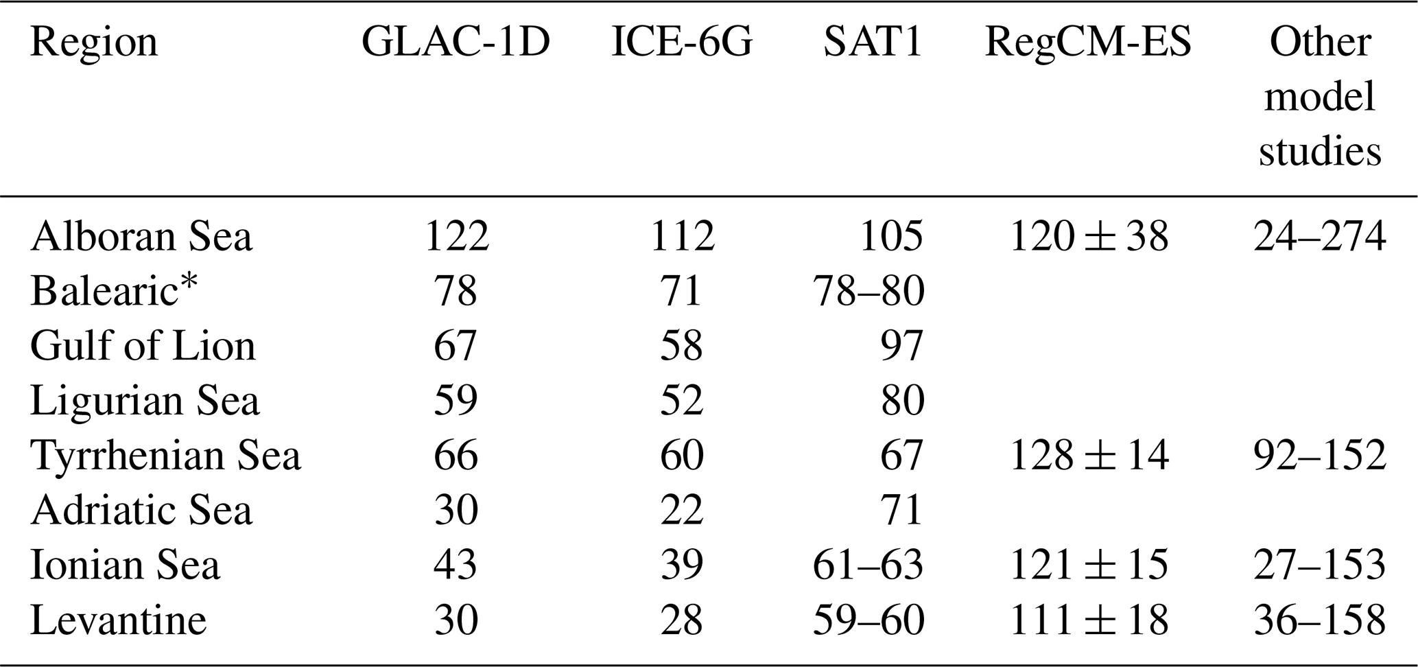
^* Balearic stands for three regions, namely the Balearic Sea, Algerian Basin, and Algero-Provençal Basin.

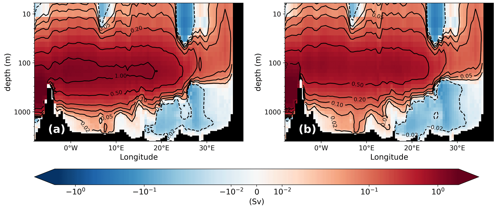
Figure A1 Mean zonal stream function (Sv) of PI of GLAC-1D (a; identical to Fig. 4a but shown again for easier comparison) and PI-Straits (b). Contour lines are given as a dashed line for (−0.02) and as solid lines for (0.02), (0.05), (0.1), (0.2), (0.5), and (1.0). Please note the logarithmic depth scale and the logarithmic colour scale.

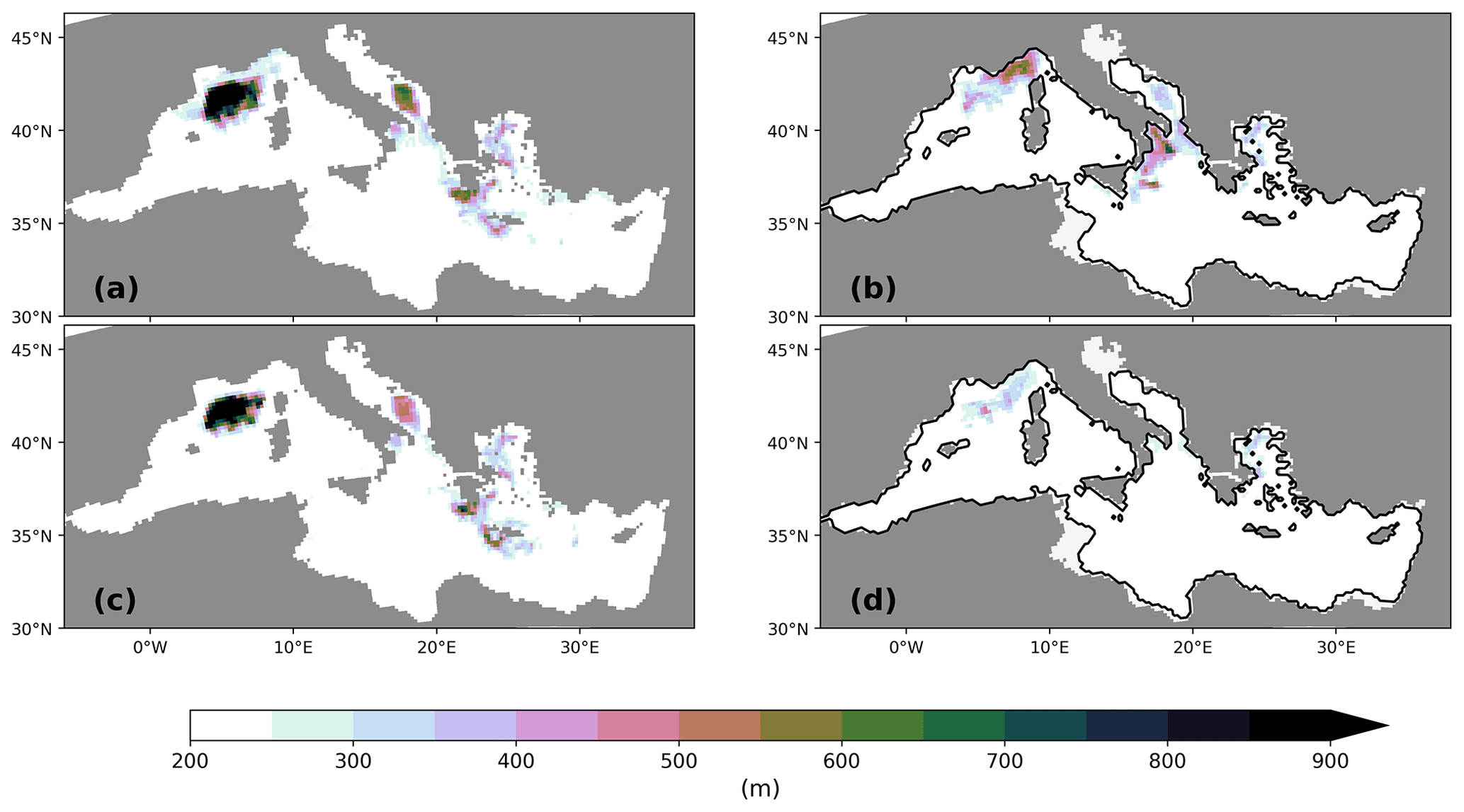
Figure A2 Maximum annual mixed layer depth (m) for the PI of GLAC-1D (a) and for the LGM of GLAC-1D (b) and ICE-6G (d). Panel (c) gives the information for PI-Straits. The contour line indicates the LGM coastline.

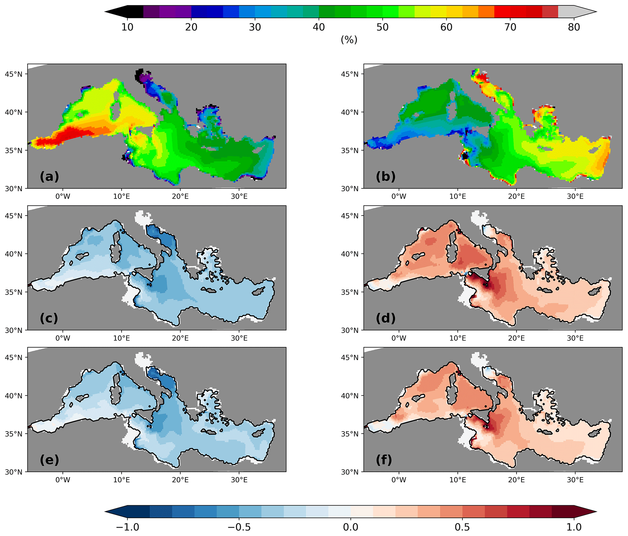
Figure A3 Weight percentage sediment contribution in the upper 6 mm of the sediment column of calcite (a) and terrestrial material, i.e. clay, (b) for the PI of GLAC-1D (in %). Relative changes between LGM and the corresponding PI are given for calcite (c, e) and clay (d, f) for GLAC-1D (c, d) and ICE-6G (e, f).

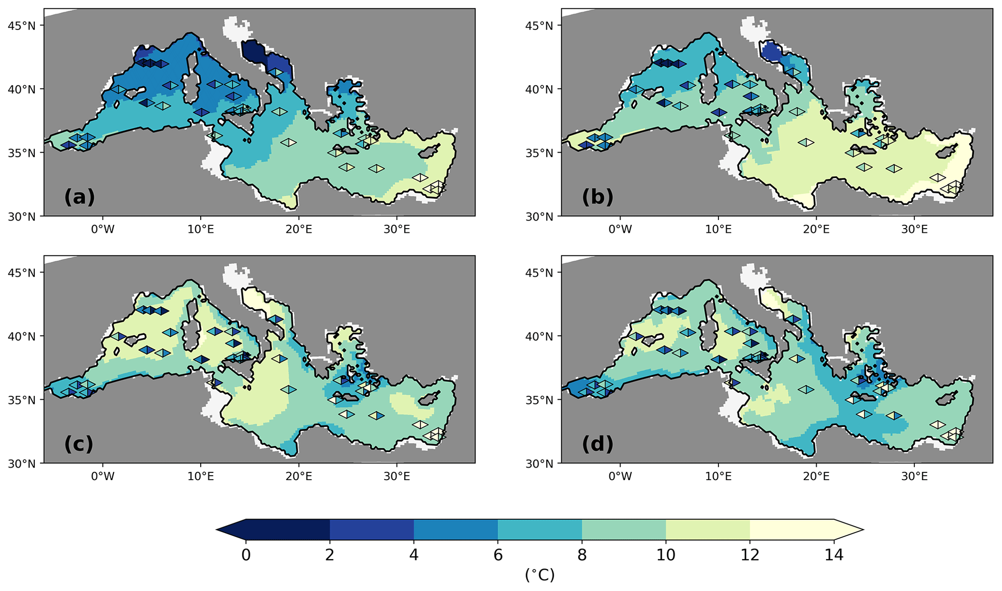
Figure A4 Annual minimum sea surface temperature (SST; a, b) and seasonal amplitude of the SST (c, d) during the LGM for GLAC-1D (a, c) and ICE-6G (b, d). Seasonal amplitude is calculated from annual maximum and annual minimum. All units are in degrees Celsius. Overlaid data from Hayes et al. (2005) for the same quantities estimated with two different methods, namely the artificial neural network (left part of the rhombus) and the revised analogue method (right part of the rhombus). See Hayes et al. (2005) for more details.

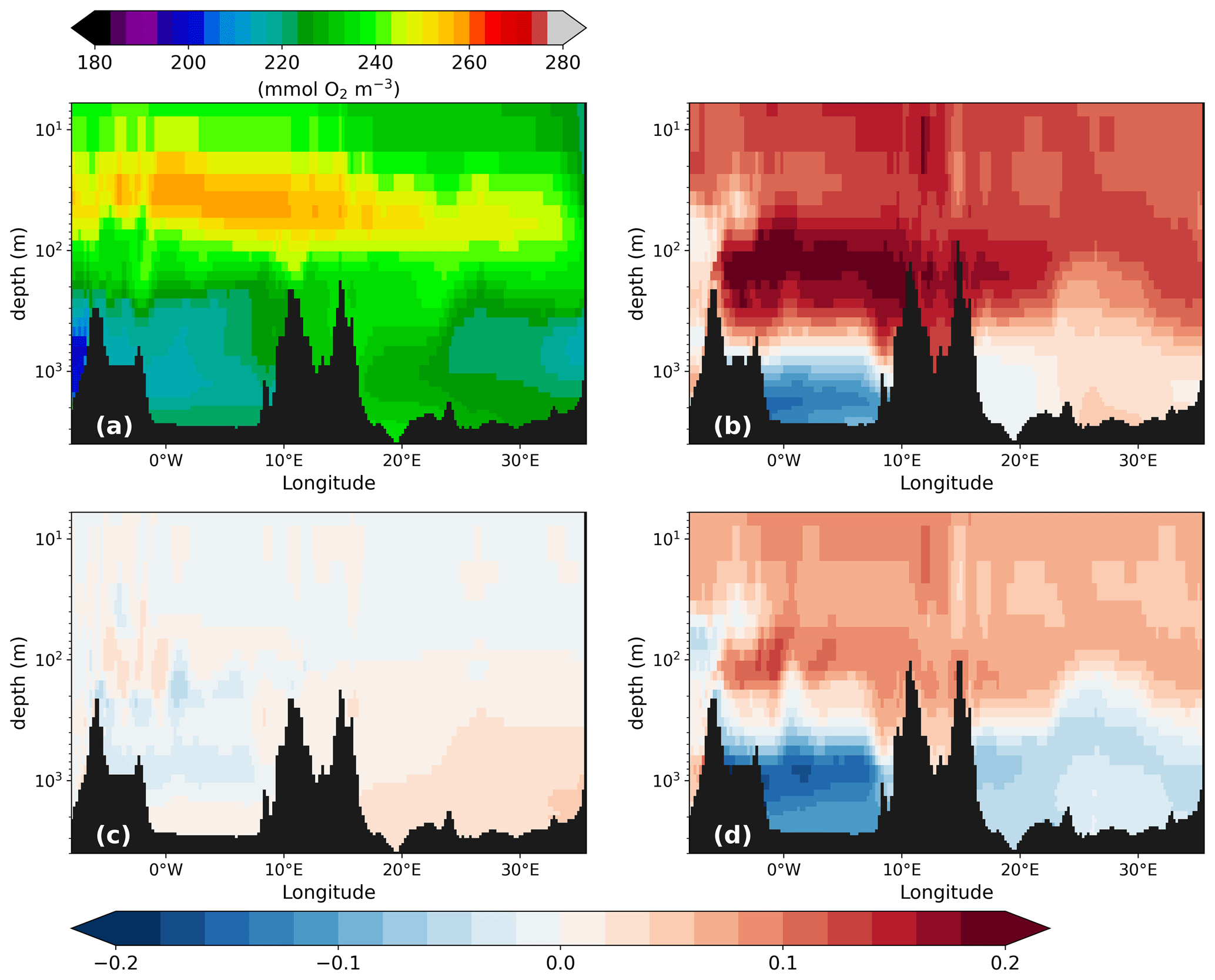
Figure A5 Similar to Fig. 13 but for oxygen concentration (mmol O₂ m⁻³) along the west–east transect (for the location, see Fig. 1) of the PI of GLAC-1D (a) and the relative concentration change between the LGM and the corresponding PI of GLAC-1D (b) and ICE-6G (d) and between PI-Straits and the PI of GLAC-1D (c). Note the logarithmic depth scale in all panels. Colder temperatures during the LGM increase the oxygen concentration in surface waters (b, d). The larger export of organic matter leads to oxygen consumption at depth, but both deep basins are still well ventilated. The almost identical climate in PI-Straits (c) is reflected in a nearly identical oxygen concentration to that in the PI. The small increase in O₂ concentrations in the eastern basin is attributable to a reduced organic matter flux at greater depth.

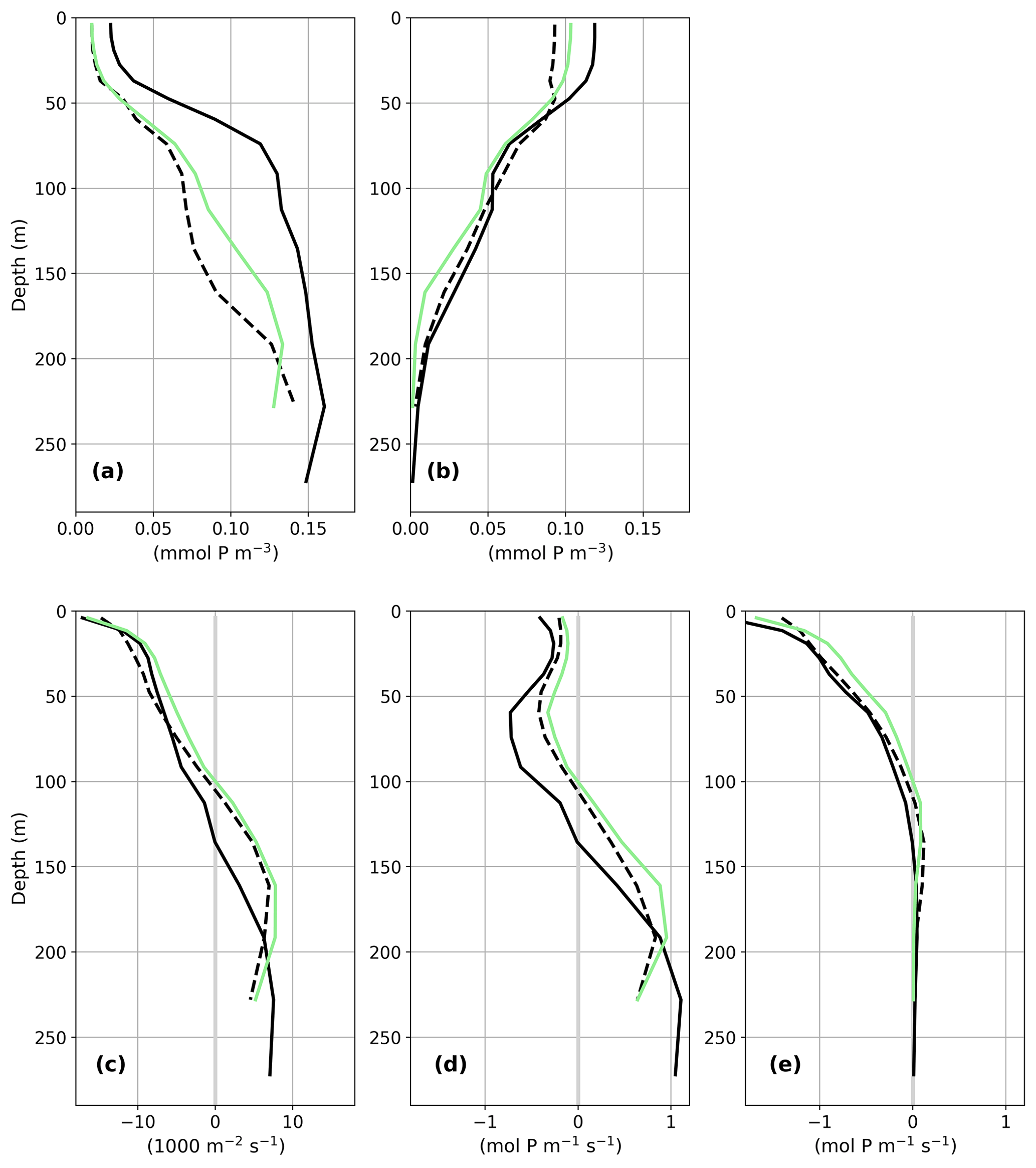
Figure A6 Concentration profiles in the Strait of Sicily for dissolved (a) and organically bound phosphate (b) (both in mmol P m⁻³), the meridional transport through the strait (c; velocity times strait width in 1000 m² s⁻¹), and the transport of dissolved phosphate (d) and of organically bound phosphate (e) (both in mol P m⁻¹ s⁻¹) which is shown as a sum in Fig. 15. Colour coding is the same as in Fig. 15 for GLAC-1D-PI (solid black line), GLAC-1D-LGM (dashed black line), and PI-Straits (green line).

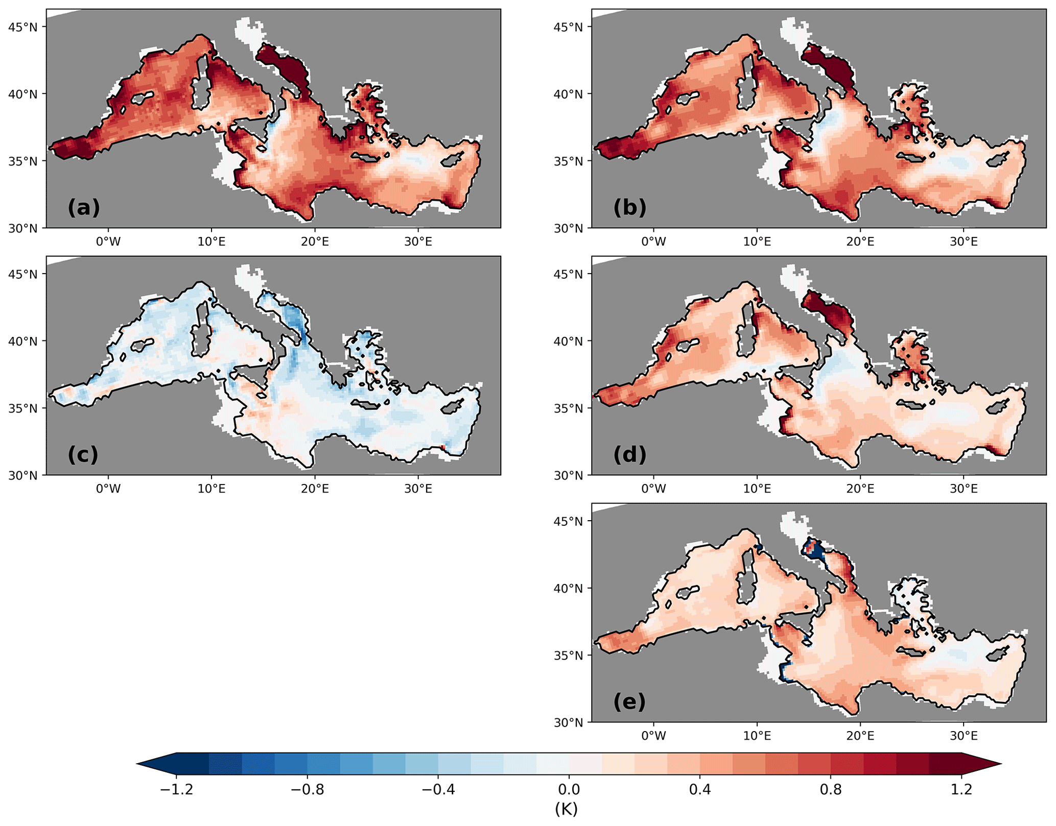
Figure A7 Same as Fig. 16 but for ICE-6G. Shown are the differences between ΔT_org and ΔT₃₂ (a), the differences between ΔPWT and ΔT₃₂ (b), and the difference between ΔPWT and ΔT_org (c). Panel (d) shows ΔPWT_NPP, the NPP-related contribution to ΔPWT, and panel (e) displays ΔPWT_T−ΔT₃₂, the temperature-related contribution. As for GLAC-1D, ΔT_org does not capture the full cooling signal given by ΔT₃₂.