Climate and ice sheet dynamics in Patagonia throughout marine isotope stages 2 and 3

During the Last Glacial Maximum (LGM, ∼ 23 000 to 19 000 years ago), the Patagonian Ice Sheet (PIS) covered the central chain of the Andes between ∼ 38 to 55° S. Existing paleoclimate evidence – mostly derived from glacial landforms – suggests that maximum ice sheet expansions in the Southern Hemisphere and Northern Hemisphere were not synchronized. However, large uncertainties still exist in the timing of the onset of regional deglaciation and its major drivers. Here we present an ensemble of numerical simulations of the PIS during the LGM. We assess the skill of paleoclimate model products in reproducing the range of atmospheric conditions needed to enable an ice sheet growth in concordance with geomorphological and geochronological evidence. The resulting best-fit climate product is then combined with records from southern South America offshore sediment cores and Antarctic ice cores to drive transient simulations throughout the last 70 ka using a glacial index approach. Our analysis suggests a strong dependence of the PIS geometry on near-surface air temperature forcing. Most ensemble members underestimate the ice cover in the northern part of Patagonia, while tending to expand beyond its constrained eastern boundaries. We largely attribute these discrepancies between the model-based ice geometries and geological evidence to the low resolution of paleoclimate models and their prescribed ice mask. In the southernmost sector, evidence suggests full glacial conditions during marine isotope stage 3 (MIS3, ∼ 59 400 to 27 800 years ago), followed by a warming trend towards MIS2 (∼ 27 800 to 14 700 years ago). However, in northern Patagonia, this deglacial trend is absent, indicating a relatively consistent signal throughout MIS3 and MIS2. Notably, Antarctic cores do not reflect a glacial history consistent with the geochronological observations. Therefore, investigations of the glacial history of the PIS should take into account southern midlatitude records to capture effectively its past climatic variability.

1 Introduction

At present, there are only two ice sheets on Earth. The Antarctic ice Sheet is the largest, with an ice volume of 26.04 ± 0.4 ×10⁶ km³ that can be translated into a sea level equivalent (SLE) of 57.0 ± 0.9 m (Morlighem et al., 2020). The Greenland Ice Sheet contains 2.99 ± 0.2 ×10⁶ km³ of ice, which corresponds to a SLE of 7.42 ± 0.05 m (Morlighem et al., 2017). However, during the last glacial period, especially during the global Last Glacial Maximum (LGM, 23 000 to 19 000 years before present, ka), much of North America was buried under the North American Ice Sheet complex, the Eurasian Ice Sheet complex stretched across most of northern Europe, and the Patagonian Ice Sheet (PIS) covered the western part of southern South America. The ice locked away in these former ice sheets represented a SLE of around 113.9 m (Simms et al., 2019). When the contributions from Antarctica and Greenland are added on top, this results in an estimated total sea level drop at of 120–134 m below present levels between 29 and 21 ka (Lambeck et al., 2014). This period was marked by partly exposed continental shelves, strong winds, dry conditions, and a total greenhouse gas concentration lower than during the pre-industrial period (PI; Monnin et al., 2001; Bartlein et al., 2011; Kohfeld et al., 2013; Simms et al., 2019), lowering the global mean surface air temperature by 3.2 to 6.7 °C with respect to the pre-industrial level (Schneider von Deimling et al., 2006; Holden et al., 2010; Annan and Hargreaves, 2013; Tierney et al., 2020; Kageyama et al., 2021).

The PIS was a relatively small ice sheet, comparable in size to the former Celtic Ice Sheet that covered the British Isles during the LGM (Hughes et al., 2016). Its former evolution is still subject to considerable uncertainties regarding ice extent, ice volume, and contribution to sea level variations, mainly due to the scarcity of geological evidence (Hulton et al., 2002; Davies et al., 2020; Wolff et al., 2023). Only recently, Davies et al. (2020) succeeded in building a geochronological data set of a reasonable size and robustness, arriving at the conclusion that the PIS reached its maximum extent during the marine isotope stage (MIS) 3 at ∼ 35 ka. This state remained nearly unchanged until 27 ka, which is much earlier than the global timing estimates for LGM. This is a generic estimate because the evidence suggests that the timing of its maximum extent changed with latitude: the northern sector located between of 38 to 48° S is thought to have reached its largest area between 33 to 28 ka, while its southern counterpart (between 48 to 56° S) peaked much earlier, at around 47 ka. Based on simplifying assumptions, Davies et al. (2020) estimated a uniform maximum PIS extent of 492 600 km² at 35 ka, corresponding to a SLE of around 1.5 m.

Recently, Yan et al. (2022) modeled the PIS extent during the LGM combining the temperature and precipitation from 21 PMIP outputs from phases 2, 3, and 4 to analyze the degree of agreement between their modeled geometries and the PATICE reconstruction (Davies et al., 2020). One of the main findings of their study is that most of the uncertainty in the modeled PIS geometry is associated with the PMIP forcing, producing an overestimation of the ice-covered extent over vast regions, while showcasing an underestimation of ice in other areas. These results reflect the inability of most PMIP model products to provide climate conditions that allow for ice sheet advance in the northernmost sectors of Patagonia during the LGM, even under a somewhat extreme choice of model parameters. Only some of the PMIP4 models seem to present the climate conditions needed to trigger ice sheet inception and growth in this region. However, Yan et al. (2022) did not provide potential reasons for these discrepancies.

In this study, we use the numerical ice sheet model SICOPOLIS (Greve, 1997; Sato and Greve, 2012) to explore the range of climate conditions that leads to a good match between the modeled PIS and field-derived geometries during the global LGM. The resulting best-fitted climate model is then used to perform transient simulations throughout MIS4 and MIS2 to explore the timing of the local maximum ice extension and the consequent deglaciation. Our ice sheet modeling experiments are driven by climate products from phases 3 and 4 of PMIP and employ the glacial index method derived from offshore records and Antarctic cores. Furthermore, we assess the relative performance of our simulations against the geochronological reconstruction of Davies et al. (2020).

2 Methods

2.1 Model setup

All numerical simulations of the PIS in this study are performed using the open source, three-dimensional, thermomechanical ice sheet model SICOPOLIS (SImulation COde for POLythermal Ice Sheets; Greve, 1997; Sato and Greve, 2012) and cover the area between 80 and 62° W and between 36 and 58° S (Fig. 1). This model domain is discretized using an equidistant grid with a horizontal resolution that ranges between 4 and 8 km, for equilibrium and transient simulations, respectively (see Sect. 2.2 and 2.3). In the vertical dimension, the grid is extruded into 81 terrain-following layers that densify towards the base, from which 3 are allocated to accommodate the potential presence of temperate ice. Within this three-dimensional grid, the model discretizes and approximates the full Stokes solution for the ice velocity field, u, using a hybrid combination of the solutions u_SIA and u_SStA from the shallow ice and shelfy stream approximations (SIA and SStA, respectively; see Bueler and Brown, 2009), following the approach described in Bernales et al. (2017):

$$\begin{array}{}\text{(1)}& \mathit{u}=(\mathrm{1}-w)\cdot {\mathit{u}}_{\mathrm{SIA}}+{\mathit{u}}_{\mathrm{SStA}},\end{array}$$

where w is a space- and time-variant weight used to reduce the contribution from the SIA in fast-flowing areas where the assumptions behind the approximation might not hold, which is computed as

$$\begin{array}{}\text{(2)}& w\left(\left|{\mathit{u}}_{\mathrm{SStA}}\right|\right)={\displaystyle \frac{\mathrm{2}}{\mathit{\pi }}}\arctan \left({\displaystyle \frac{{\left|{\mathit{u}}_{\mathrm{SStA}}\right|}^{\mathrm{2}}}{u_{\mathrm{ref}}^{\mathrm{2}}}}\right).\end{array}$$

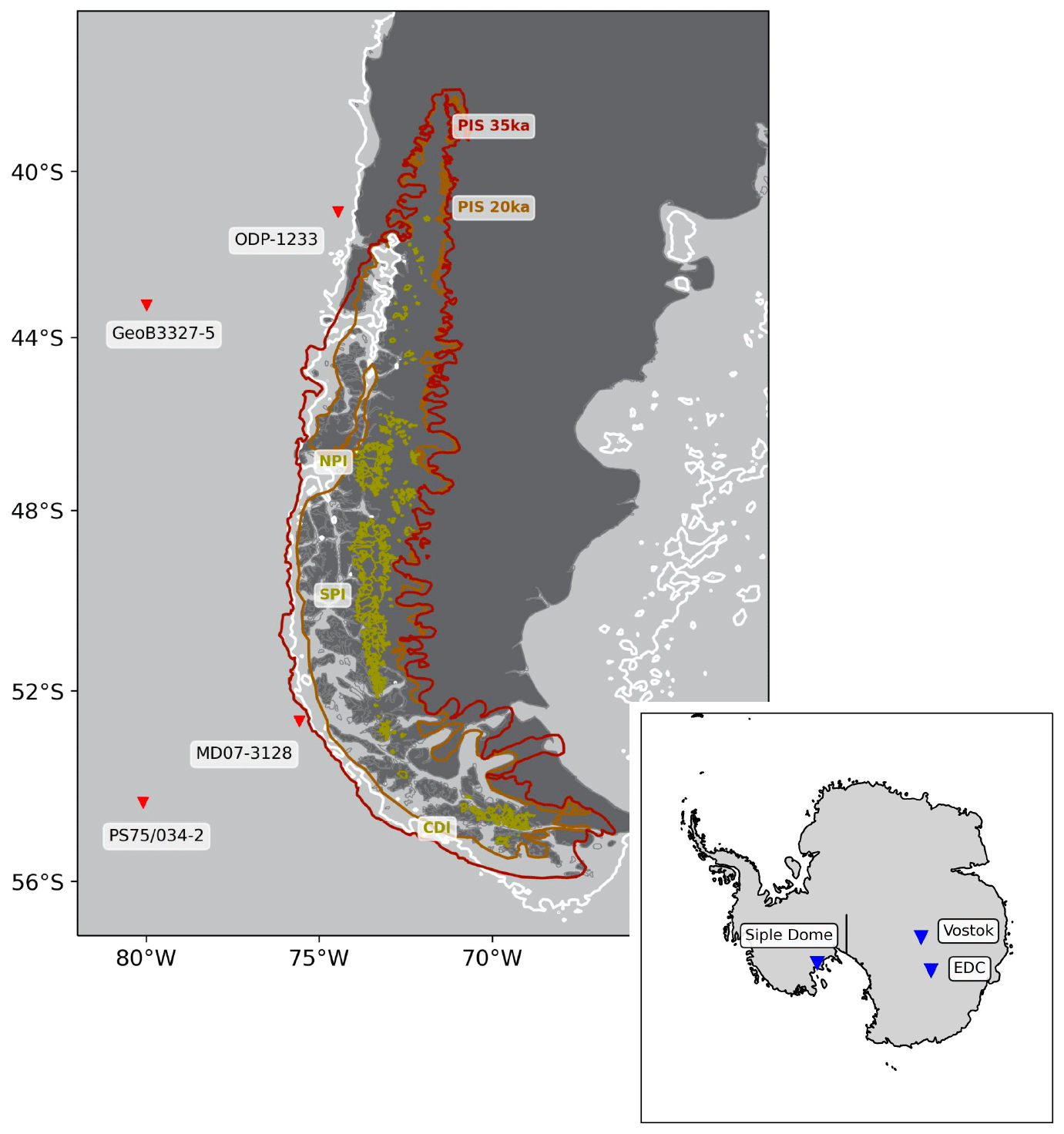
Figure 1 PIS reconstruction of Davies et al. (2020) for 35 and 20 ka. Present-day ice fields are indicated and correspond to the Northern Patagonian Ice Field (NPI), Southern Patagonian Ice Field (SPI), and Cordillera Darwin Ice Field (CDI). LGM coastal lines marking the lower sea level (−120 m) are shown in white.

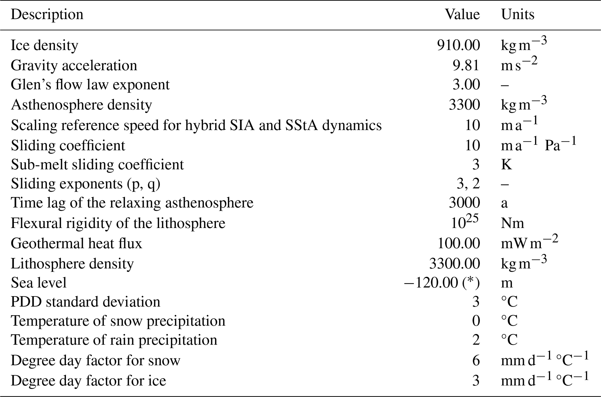
Here, u_ref is a reference ice speed at which the SIA contribution is halved (see Table 1) that is used to roughly represent the onset of significant basal sliding under ice streams. This hybrid model solves for an ice velocity field that corresponds to a given ice geometry, mass balance, and thermal state. The resulting velocity field is then used to compute the evolution of ice within the domain by integrating the model forward in time under a time step that ranges between 0.5 and 1 year, depending on the horizontal grid resolution applied. We use a Weertman-type power law as in Sato and Greve (2012) to enable sliding at the base of the ice at locations where the base is close to its local pressure melting point:

$$\begin{array}{}\text{(3)}& {\mathit{u}}_{\mathrm{b}}=-{\displaystyle \frac{C_{\mathrm{b}}}{N_{\mathrm{b}}^q}}{\left|{\mathit{\tau }}_{\mathrm{b}}\right|}^{p-\mathrm{1}}{\mathit{\tau }}_{\mathrm{b}},\end{array}$$

where u_b and τ_b are basal ice velocity and basal shear stress, respectively; p and q are sliding law exponents (see Table 1); and N_b is the overburden basal pressure exerted by the ice column. In this sliding law, basal hydrology contributes to a reduction in the overburden pressure depending on the difference between the local bedrock elevation and sea level, similar to the approach in Martin et al. (2011). In Eq. (3), C_b is a scaling factor assumed to depend on basal thermal conditions:

$$\begin{array}{}\text{(4)}& C_{\mathrm{b}}=C_{\mathrm{0}}\cdot e^{\frac{T_{\mathrm{m}}}{\mathit{\gamma }}},\end{array}$$

where T_m is the ice temperature relative to the pressure melting point and C₀ and γ are sliding parameters (see Table 1). Grounded ice is allowed to advance until the coast, beyond which any further advance into the ocean is prevented; i.e., we do not allow for the formation of ice shelves. Therefore, potential effects caused by the ocean thermal forcing are not included. Since we utilize a hybrid combination of the shallow ice and shallow shelf approximations, ice streams can form.

Table 1 The most important parameters in the model setup. (^*) For transient simulations, the SPECMAP sea level reconstruction has been used.

At the beginning of each simulation, an ice-free topography is prescribed and mapped onto the horizontal model grid based on the ETOPO1 data set (Amante and Eakins, 2009). Within this bedrock, a lithospheric model layer is represented by an extension of the extruded horizontal grid spanning 41 additional vertical points. At the base of this layer, a constant, spatially homogeneous geothermal heat flux of 100 mW m⁻² is applied, in agreement with averaged values observed in Patagonia (Hamza and Vieira, 2018), which serves as the lower thermodynamical boundary condition for the model. Glacial isostatic adjustment of this bedrock produced by temporal variations in the ice mass load is accounted for through an elastic lithosphere–relaxing asthenosphere (ELRA) model (e.g., Greve and Blatter, 2009) using standard parameter values (see Table 1).

This initialization assumes a global sea level drop of 120 m based on reconstructions for the LGM (Lambeck et al., 2014), which is applied homogeneously over the entire model domain. The ice is only allowed to advance on land, being immediately calved out on the coast. Ocean temperature and dynamics beyond the sea level change have no implication whatsoever in our simulations.

The inception and evolution of the PIS in our model is driven by the surface mass balance (SMB), which is calculated as the difference between applied fields of accumulated precipitation and surface ablation. The latter is computed using a positive-degree-day (PDD) model following Calov and Greve (2005), based on a given near-surface air temperature field and the parameters in Table 1. PDD values have been selected based on contemporary and paleo-studies in the area (Fernández and Mark, 2016; Yan et al., 2022; Cuzzone et al., 2024). Surface mass accumulation is assumed to depend on monthly precipitation and temperature fields, such that the transition between solid and liquid precipitation is linearly proportional to variations in air temperature (Marsiat, 1994). Here we use a transition range of 0 to 2 °C, producing purely solid or purely liquid precipitation below or above this temperature range, respectively. As the model domain surface evolves due to the advance and retreat of the PIS during a simulation, discrepancies between the prescribed (fixed) topography used in the PMIP climate model snapshots and the dynamic one in SICOPOLIS are accounted for by implementing a near-surface air temperature lapse-rate correction of −6.5 K km⁻¹. The precipitation change a 7.3 % for each degree Celsius of air temperature change (Huybrechts, 2002). The resulting atmospheric temperatures near the surface of the ice are then applied as the upper thermodynamical boundary conditions.

2.2 Equilibrium simulations at the global LGM

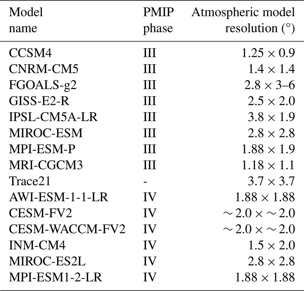
Starting from the ice-free conditions described in Sect. 2.1, an ensemble of model simulations is run forward in time, each member forced by a different pair of matching near-surface air temperatures and total precipitation fields from 15 climate models that participated in the LGM experiments during phases 3 and 4 of PMIP. A list of these climate models is presented in Table 2. The forcing fields contained in a given LGM climate snapshot are applied in a constant manner, i.e., without any temporal variations as the domain evolves, except for the lapse-rate correction and elevation desertification described in Sect. 2.1. In areas where a temperature–precipitation pair results in a positive SMB, inception of ice will occur. The ice mass will then grow and advect outwards, leading to an advance of the emerging PIS. The extent of this advance will be limited by areas where a negative SMB fully compensates for the advected ice from upstream. As the PIS thickens, the amount of ice transported downstream increases, while surface ablation decreases due to the cooling of near-surface temperatures as a result of the lapse-rate correction. This positive feedback is then balanced by a reduction in the available precipitation as elevation desertification sets in. As the model is integrated forward in time, these competing effects shape the advancing PIS until a balance between the accumulation and ablation zones of the entire ice sheet is reached. Each equilibrium simulation in this study spans 10 000 model years, which is enough to bring the domain to a steady state under each of the time-invariant climate conditions. The resulting PIS geometry for each of the ensemble members is evaluated against the LGM snapshot (20 ka) from the PATICE geological reconstruction (Davies et al., 2020) in Sect. 3.

Table 2 Climate models analyzed in the present study.

2.3 Transient simulations through MIS3 and MIS2

The equilibrium simulations described in Sect. 2.2 assume constant, peak glacial conditions from PIS inception to steady state. These assumptions introduce a cold bias in both the internal thermal regime of the ice sheet and the applied SMB. For the former, the influence of warmer or colder past climates on englacial conditions can last for tens of thousands of years after such conditions have disappeared, given the slow response timescales of ice sheets (Rogozhina et al., 2011).

With the aim of reducing the biases mentioned above and explore the glacial history of the PIS before the global LGM, we perform a second ensemble of simulations using transient climate forcing. This forcing is derived by first selecting the best-performing member from the equilibrium ensemble of simulations (see Sect. 3) based on assessments of both area coverage and temporal responsiveness to evolution. Following this, for each climate model the LGM condition is complemented by a corresponding PI, representing peak glacial and interglacial conditions, respectively:

$$\begin{array}{}\text{(5)}& {\displaystyle }T\left(t\right)=T_{\mathrm{PI}}+\mathrm{GI}\left(t\right)\cdot (T_{\mathrm{LGM}}-T_{\mathrm{PI}})\text{(6)}& {\displaystyle }P\left(t\right)=P_{\mathrm{PI}}\cdot \left(\mathrm{1}-\mathrm{GI}\left(t\right)\cdot \left(\mathrm{1}-{\displaystyle \frac{P_{\mathrm{LGM}}}{P_{\mathrm{PI}}}}\right)\right),\end{array}$$

where T and P represent the temperature and precipitation fields through time, respectively. In order to generate a climate state at any given model time, these two snapshots are then subjected to a weighted interpolation following a glacial index (GI) approach

$$\begin{array}{}\text{(7)}& \mathrm{GI}\left(t\right)={\displaystyle \frac{\mathit{\delta }X\left(t\right)-\mathit{\delta }{X}_{\mathrm{PI}}}{\mathit{\delta }{X}_{\mathrm{LGM}}-\mathit{\delta }{X}_{\mathrm{PI}}}},\end{array}$$

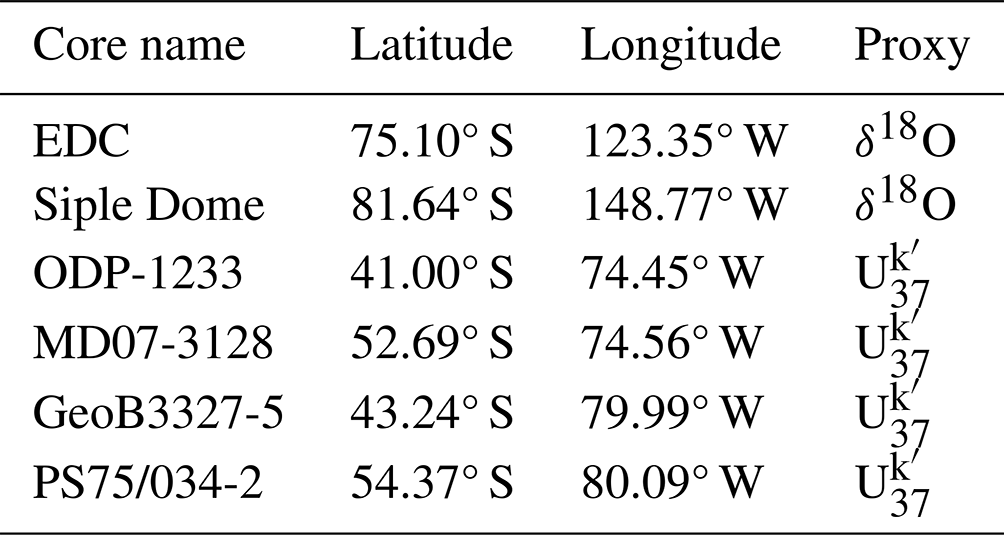
where t is time and X is the sea surface temperature derived from ${\mathrm{U}}_{\mathrm{37}}^{{\mathrm{k}}^{\prime }}$ for the offshore records and δ¹⁸O for the ice core records (e.g., Mas e Braga et al., 2021). Here, the time-dependent weight is in turn derived from a list of ice and offshore sediment cores (see Table 3). For all core records, the computation of the GI uses the 19–23 ka mean of either δ¹⁸O (for ice cores) or sea surface temperature (SST; for sediment cores) to define peak glacial conditions. Likewise, peak interglacial conditions are defined against a near-PI period by averaging over the last 3 ka. The latter is, however, not possible for the GeoB3327-5 and PS75/034-2 sediments cores, which lack late Holocene data. For these two cores, values from the centennial-timescale SST reconstruction COBEV2 (Ishii et al., 2005) have been used to fill the data gap. With this range of far- and near-field core locations, we investigate whether the offshore records along the Pacific margin contain any imprints of an earlier, local glacial maximum in the Patagonian region. Each of the simulations in the transient ensemble is initialized from ice-free conditions and keeping the setup of the equilibrium ensemble as described in Sect. 2.2, except for the climate forcing. Following this, each member is run under a different record-derived GI spanning the period between 70 ka and PI, encompassing both MIS3 and MIS2.

Table 3 Core records used for the glacial indexes.

3 Results

3.1 Performance of the PMIP models at the LGM in Patagonia

Our equilibrium model experiments produce a wide range of PIS geometries, some of which are generally comparable with the geologically constrained ice extents, while others yield considerably reduced and/or overextended ice cover (Fig. 5). We have divided the former PIS extent into three distinct latitudinal ranges based on their model sensitivity and response to the imposed climate. Each of these areas is described and analyzed in detail in the following sections. First, south of 52° S, most ensemble members exhibit an unrealistic buildup of ice in southeastern Patagonia, with a much larger ice-covered area than inferred from the geological evidence. Second, between 44 and 52° S, a continuous ice sheet growth is reached by nearly all ensemble members, with an overall good match for both the eastern and western margin of PATICE. Finally, in the third zone between 38 and 44° S, PIS growth is not uniformly captured by the ensemble members, with most of them failing to build a consistent ice cover.

Among the PMIP climate model products tested in this study, AWI-ESM-1-1-LR and MPI-ESM1-2-LR models (both from PMIP4) produce the most consistent ice sheet extents relative to the PATICE reconstruction (Fig. 1). However, MPI-ESM1-2-LR's near-surface air temperature allows faster growth when compared to AWI-ESM-1-1-LR, having a better performance in the transient experiments. However, they exhibited disparities in their temporal responses to growth. Notably, AWI-ESM-1-LR displayed a slower growth pace attributed to its temperature field. This slower growth response during the LGM has led to an unrealistic configuration of the ice sheet when performing transient simulations under the model configuration chosen in this study. The near-surface air temperature and precipitation patterns derived from these two climate models enable the modeled ice sheet to reach as far north as 39 and 40° S, respectively, and occupy total areas of 467 776 and 564 096 km². This is in broad agreement with the earlier estimations by Davies et al. (2020). Total ice volumes produced by these two simulations are 347 020 and 471 859 km³, corresponding to SLEs of 1.04 and 1.37 m (Fig. 5), respectively. In the following, we zoom in on the drivers of the dissimilar model performances across these three distinct zones.

3.1.1 Excessive Patagonian ice cover in southeastern Patagonia

Our model experiments show that across southern Patagonia (52 to 56° S) most ensemble members exhibit an unrealistic buildup of ice, with a much larger eastern ice extent than inferred from the geological evidence (Fig. 5). In some cases (e.g., ensemble members driven by CCSM4, GISS-E2-R, MIROC-ESM, Trace21ka, CESM2-FV2, and CESM2-WACCM-FV2), this excessive ice cover reaches what is at present the Atlantic coast. We associate the excessive growth towards the eastern side with relatively cold conditions on the leeward side of the Andes (Figs. 2, 4), accompanied by relatively large precipitation amounts when compared with the multi-model mean. These climate conditions reduce the ablation, allowing the ice sheet to advance beyond the margins of the PATICE reconstruction.

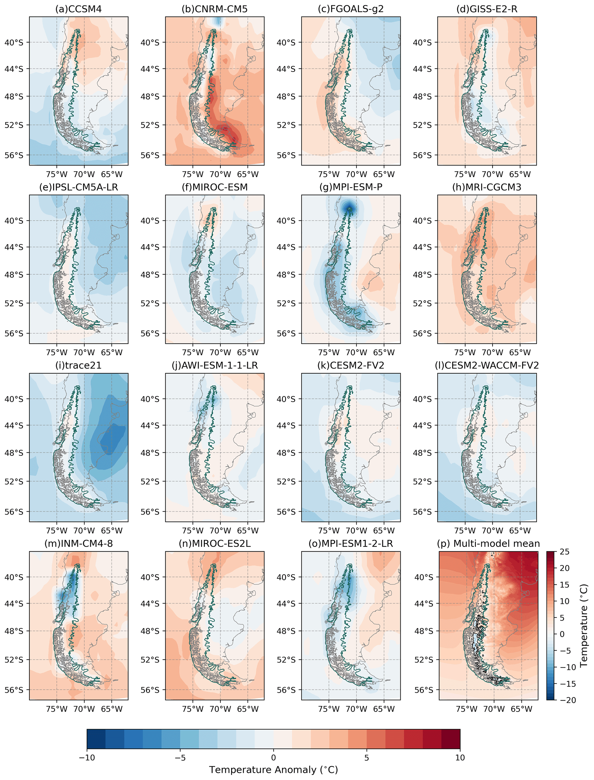
Figure 2 (a–o) LGM summer mean temperature anomaly with respect to the LGM multi-model summer mean temperature shown in (p).

Ensemble members that reproduce an extension comparable with the geological reconstruction of PATICE showcase positive LGM temperature anomalies of around 2 °C, combined with drier conditions with respect to LGM multi-model mean east of the geologically reconstructed margin of the PIS (Figs. 2, 3; see climate models AWI-ESM-1-1-LR, MPI-ESM1-2-LR, and CNRM-CM5).

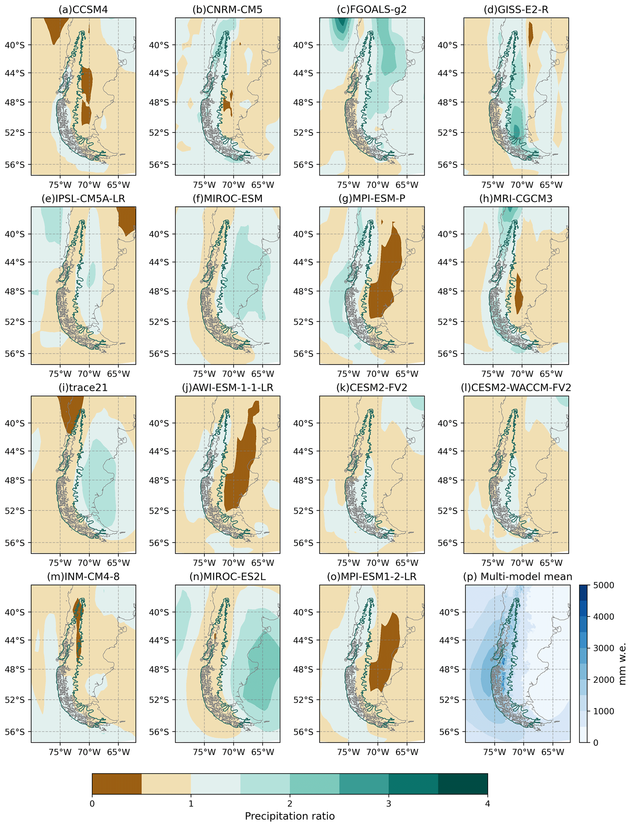
Figure 3 (a–o) LGM total annual precipitation ratio with respect to the LGM multi-model mean of the total annual precipitation shown in (p).

3.1.2 Ice sheet extents and climate uncertainty in central Patagonia

Between 44 and 52° S, the model ensemble shows a relatively low sensitivity to the climatic uncertainty provided by the PMIP models used in this study. A continuous ice sheet buildup is reached by most ensemble members, with an overall good match along both the eastern and western margins constrained by the PATICE data. Although temperature and precipitation within the margins of the geologically reconstructed PIS at these latitudes show a large spread (Figs. 2, 3, 4), this does not lead to drastic changes in the resulting ice sheet extents. The eastern expansion of the modeled PIS seems to be linked to the summer temperature in eastern Patagonia, inhibiting the melting during the summer season, despite the reduced precipitation (Fig. 3). The forcing from MIROC-ES2L generates LGM climate conditions that lead to the smallest PIS in the ensemble. Due to relatively high air temperatures, all snow accumulated during a model year is lost during the ablation season, preventing ice sheet growth and thus an extent that matches the PATICE reconstruction.

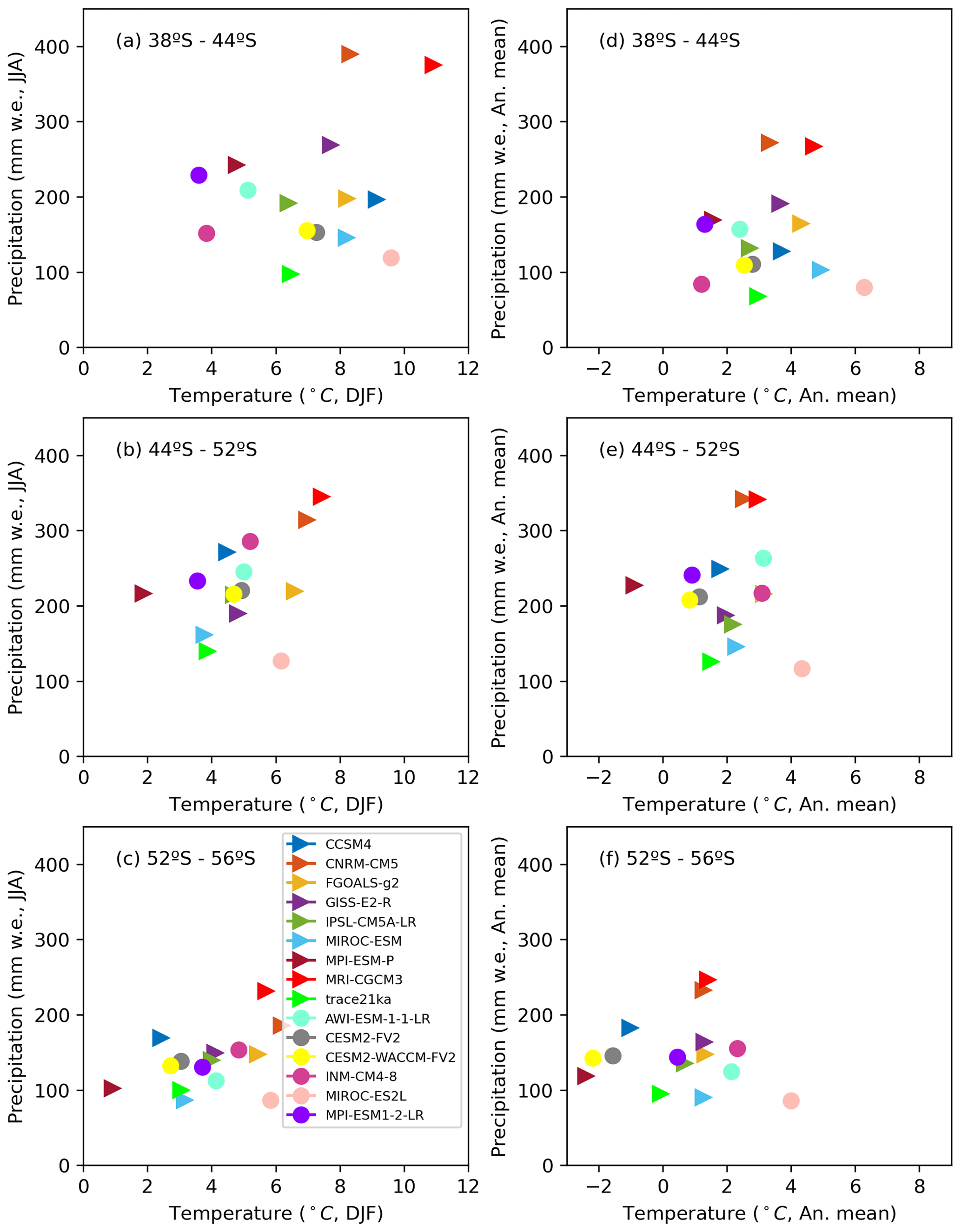
Figure 4 Scatterplot of the summer mean temperature (DJF) and the winter precipitation (JJA) and of the annual mean temperature and annual mean precipitation between (a, d) 38 to 44° S, (b, e) 44 to 52° S, and (c, f) 52 to 56° S. Averages were taken within the geochronologically constrained PIS for 20 ka. (Davies et al., 2020).

3.1.3 Drivers of the lack of ice in northern Patagonia

The PIS growth towards its northern confines is not uniformly captured by the ensemble. Most of the PMIP climate products tested here do not allow for an ice sheet expansion north of 44° S (Fig. 5), while the geologically constrained northern ice sheet margin is placed at 38° S (Davies et al., 2020). As stated earlier, positions of the former PIS margins derived using the AWI-ESM-1-1-LR, INM-CM4-8, MPI-ESM-P, and MPI-ESM1-2-LR products are closer to those inferred from the PATICE data set on its northern margin. However, the forcing from MPI-ESM-P in this area produces a fragmented ice cover that resembles an isolated ice cap disconnected from the main ice sheet (Fig. 5).

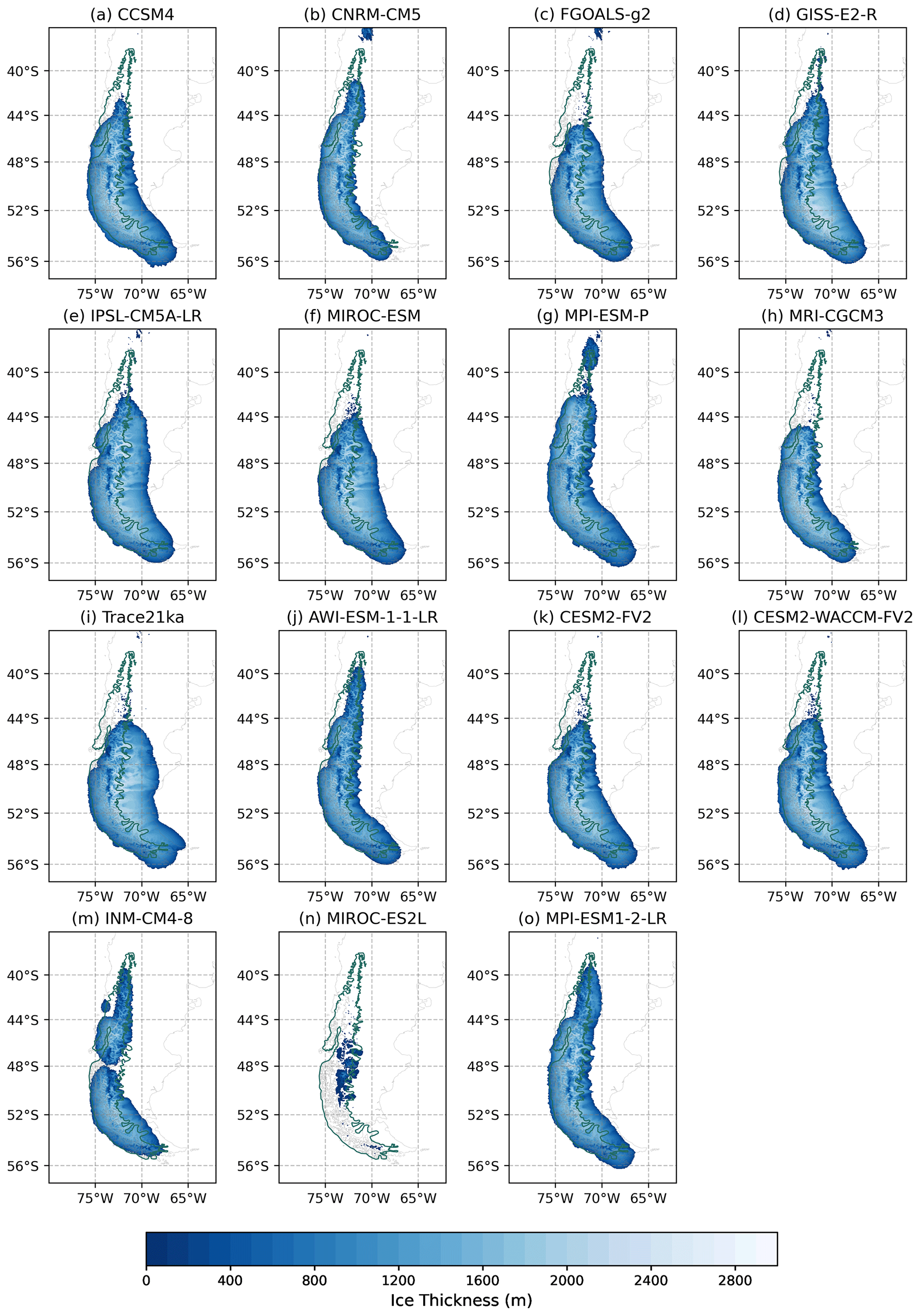
Figure 5 Modeled thickness of the PIS (m). The green line shows the reconstructed glacier extent from the empirical evidence at 20 ka (Davies et al., 2020). The present-day coastline is shown for reference.

The modeled climate from INM-CM4-8 showcases a pronounced reduction in precipitation rates during the LGM, with a decline of up to −50 % around 40° S, leading to significantly drier LGM conditions (Fig. 3). Conversely, AWI-ESM-1-1-LR, MPI-ESM-P, and MPI-ESM1-2-LR indicate relatively wetter conditions than INM-CM-8, accompanied by a comparable ice sheet extent. Meanwhile, MRI-CGCM3 depicts the highest precipitation amounts in the zone, albeit with ice-free conditions. Despite these significantly wetter conditions (25 % to 50 % larger precipitation rates than in the INM-CM4-8 model), these ensemble members fail to initiate an ice sheet in this region.

In the same latitude range, models with ice extent comparable to the geological reconstruction consistently depict colder LGM summer mean temperatures than the multi-model mean, with temperature anomalies ranging from −3 to −6 °C relative to the multi-model mean. INM-CM4-8 shows a much larger temperature anomaly, reaching −10 °C around 40° S. However, this anomaly diminishes towards the northernmost margin of the PIS, preventing ice sheet growth there under precipitation-starved conditions (Fig. 3). In this part of Patagonia, climate forcings from AWI-ESM-1-1-LR, INM-CM4-8, and MPI-ESM1-2-LR thus stand out as the only PMIP model products providing atmospheric conditions that enable the growth of an ice sheet in agreement with the PATICE data set.

Our results highlight the critical role of the summer mean temperatures in the inception and expansion of the PIS over the northern sector. Drier but colder climate states can foster ice sheet advance, while wetter yet warmer climates tend to impede ice accumulation despite relatively high precipitation rates (Figs. 2, 3). These results underscore the importance of minimizing modeled temperature biases for robust model-based reconstructions of Patagonian glacial history.

3.2 Evolution of the PIS through MIS3 and MIS2

The timing of the local maximum in terms of the ice extent and the subsequent deglaciation has been documented at multiple locations in Patagonia and recently compiled in Davies et al. (2020). This data set indicates that the former PIS reached its maximum extent at around 35 ka, preserving relatively stable conditions until 25 ka. Here we use the PMIP4 climate model MPI-ESM1-2-LR as the best-fit model to perform our transient simulations (see Sect. 2.3). For a better spatial comparison, we show the modeled extension of the PIS at 35, 30, 25, and 20 ka to enable a direct evaluation against the corresponding time slices from the PATICE reconstruction (see Sect. 2.3, Fig. 6).

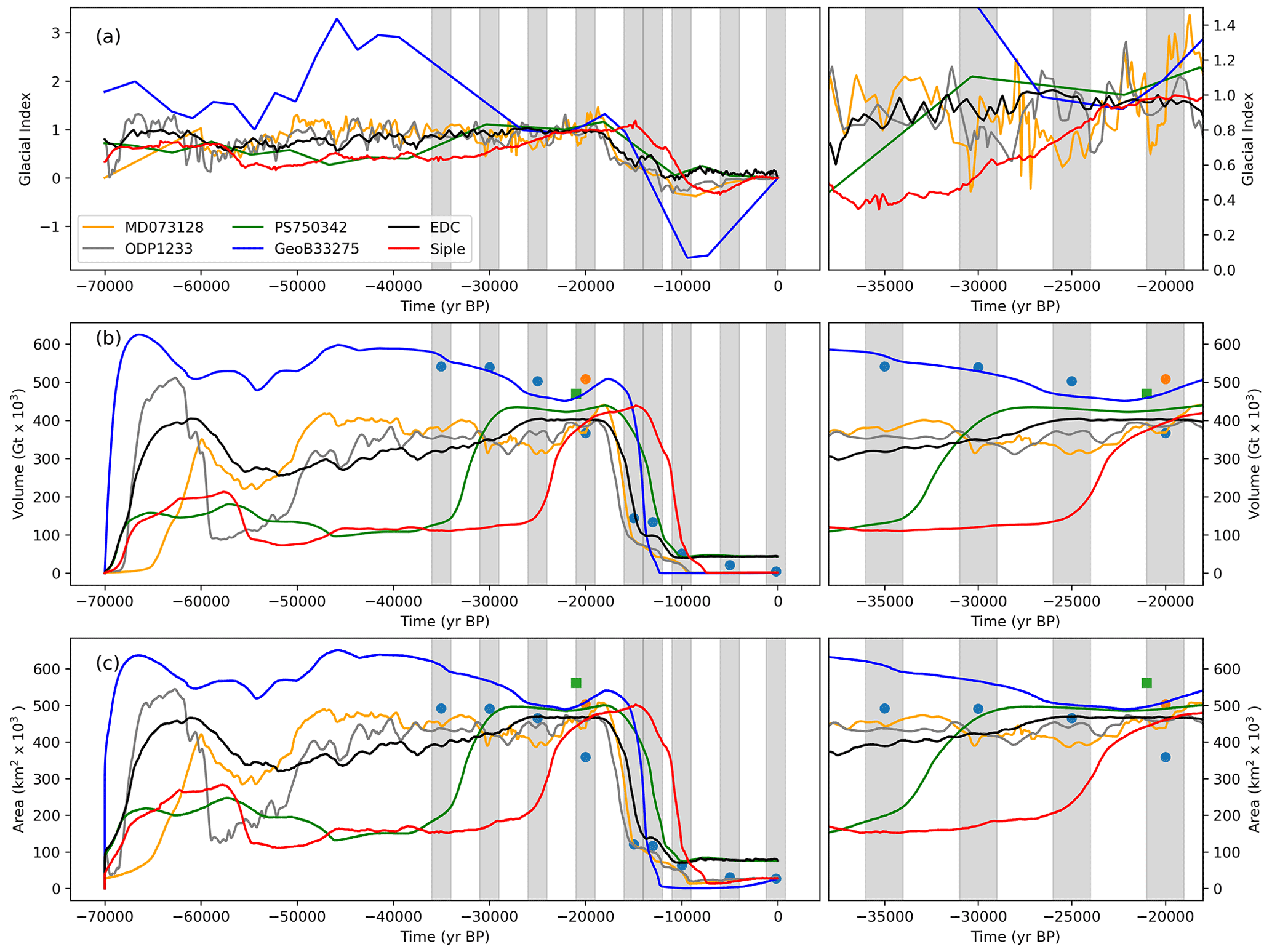
Figure 6 (a) Glacial indexes used in this study. Modeled (b) ice volumes and (c) glaciated area using MPI-ESM1-2-LR combined with the different cores used in this study (Table 3). Blue and orange circles indicate the volume and area obtained by Davies et al. (2020) and Wolff et al. (2023), respectively. Green squares indicate the modeled area and volume using MPI-ESM1-2-LR in the equilibrium simulations.

The cores ODP-1233 and MD07-3128 show quite a similar pattern, with a low glacial index during the beginning of MIS3, and they then reach ∼ 1.3 during 45 and 50 ka, respectively. Subsequently, both records demonstrate local fluctuations ranging between 0.6 to 1.3. The glacial index derived from MD07-3128 exhibits a slightly negative trend from 50 to 25 ka before experiencing an increase, reaching peak values at 20 ka. Despite their geographical separation, both cores depict transitions from glacial to interglacial conditions almost concurrently, indicating a robust regional capture of PIS dynamics (Fig. 6). Both simulations lack ice in northern Patagonia (at the northern tip) and are generally smaller than the geological reconstruction of PATICE at 35, 30, and 25 ka (Fig. 7). Nevertheless, during the LGM (Fig. 6) the ice volume ranges between the estimates by Wolff et al. (2023) and PATICE (Davies et al., 2020).

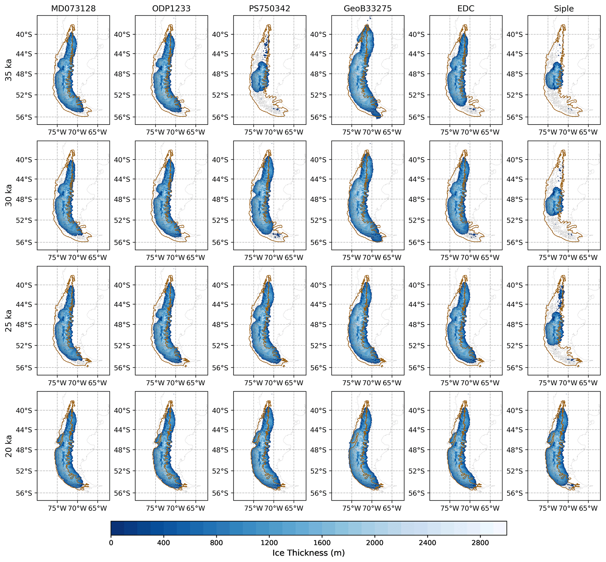
Figure 7 Modeled thickness of the PIS (m) forced by the different cores used in this study. The orange line shows the reconstructed glacier extent from the empirical evidence at 20 ka (Davies et al., 2020). The present-day coastline is shown in grey for reference.

The offshore record GeoB3327-5 shows the highest glacial index prior to the LGM, reaching maximum values of 3.3 at ∼ 45 ka, declining until it reaches values below 1 at around 18 ka (Fig. 6). Our transient simulations forced by this offshore record showcase similar ice volumes for the time slices at 35, 30, and 25 ka to those proposed by PATICE (Fig. 6). However, the region covered by the ice sheet does not completely match the geological reconstruction, overestimating the extent in northeastern Patagonia in several time slices (Fig. 7).

The offshore record PS75/034-2 shows a glacial index in the range of 0.3–0.6 between 70 and 40 ka, with a steady increase between 38 and 30 ka that brings the glacial index to a value above 1, reaching a maximum at ∼ 18 ka, and finally followed by a rapid drop (Fig. 6). These conditions lead to a small ice sheet at 35 ka, which is still growing by 30 ka, with a more stable condition between 25 and 20 ka when it reached a closer extent to the PATICE reconstruction (Fig. 7) with an ice volume of 400 000 km³, which is between the two most recent estimations (Fig. 6).

Our results using Antarctic records (EDC and Siple) suggest a maximum ice volume of the PIS closer to the global LGM, characterized by continuous ice mass growth between MIS3 and MIS2 (Fig. 6). On the one hand, the Siple Dome ice core shows glacial index values below 0.5 during most of MIS3, with an increase that begins at 30 ka, reaching a value of 1 around 20 ka and a maximum even later closer to 15 ka. These conditions lead to a small PIS during MIS3 with an ice volume of 100 000 km³ until 25 ka, when the ice sheet starts to increase, reaching 400 000 km³ at 20 ka. However, the maximum extension and volume are reached even later at 15 ka. On the other hand, EDC shows a glacial index that starts to increase during the beginning of MIS3, reaching a maximum at 25 ka, with values that keep closer to 1 until 18 ka, marking a change in its trend with an abrupt decrease. In terms of ice volume, our simulation achieves stable conditions between 25 to 18 ka with 380 000 km³. While the extension reproduced at 20 ka is reasonable, both cores exhibit a completely different glacial history when compared with the geochronological data set of PIS (Fig. 7).

4 Discussion

4.1 Performance of PMIP models in Patagonia

At the sub-regional scale, most PMIP models fail to reproduce the climate conditions required to simulate the extent of the northernmost sector of the PIS during the LGM as suggested by reconstructions. As we show in Sect. 3, the models that produce the most realistic extents of the PIS between 38–44° S are those that exhibit the coldest LGM climate during the melting season. The models AWI-ESM-1-1-LR, INM-CM4-8, and MPI-ESM1-2-LR generate larger negative temperature anomalies during the melting season when compared with respect to the multi-model mean (Fig. 2). In particular, INM-CM4-8 stands out by producing very cold conditions during the LGM nearly throughout the entire year, with a higher amplitude during January and February (austral summer) (Figs. 2, 8). Lower temperatures inferred from INM-CM4-8 act as a driving mechanism for an ice sheet growth between 38–44° S. Although the forcing fields from other models such as MPI-ESM-P and CNRM-CM5 manage to build up ice towards the north of the domain – again due to relatively colder conditions – the resulting glaciated areas resemble isolated ice caps rather than an extension of the PIS (Fig. 2). Despite colder conditions, the simulations driven by these models are still unable to reconstruct the formerly PIS-covered territories north of 39° S.

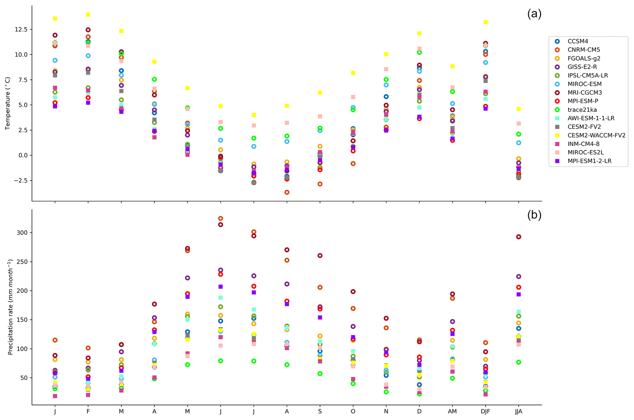
Figure 8 LGM temperatures (a) and precipitation (b) for the monthly output of CMIP5-PMIP3 and CMIP6-PMIP4 calculated of the northernmost sector of the former PIS. Calculations are made over the grid points that match the reconstructed PIS extents by Davies et al. (2020) within the 38–44° S study zone.

Similarly, the eastern expansion is consistently associated with a negative temperature anomaly when compared with respect to the multi-model summer mean (Fig. 2). As shown by the simulation driven by CNRM-CM5, relatively warm conditions are required in the southeastern sector of Patagonia to restrict the extension of the PIS within its geologically reconstructed margins (Fig. 2); this is coincidentally the model that shows the best fit in this zone. Compared to air temperatures, precipitation does not seem to play a dominant role when analyzing the causes for PIS over-expansion in this region.

The forcing from MIROC-ES2L produces the smallest modeled ice sheet geometry among all the climate models considered in this study (Fig. 5). Its summer mean temperature is the warmest, only comparable with MRI-CGCM3. Differences between the two resulting ice sheets can be explained by dissimilar summer and winter temperatures, as well as the precipitation rate (specially in winter), which in the case of MIROC-ES2L restricts accumulation during the cold season, preventing a realistic buildup (Figs. 2, 3, 8).

Previously, Yan et al. (2022) analyzed 21 PMIP model outputs of phases 2, 3, and 4 to infer the climate conditions for ice sheet growth. Despite efforts to fuse PMIP models with present-day data, models struggled to reproduce ice sheet extent accurately, showing a lack of ice in the north and overexpansion in the southeast. Cuzzone et al. (2024) investigated PMIP4 models in a narrower domain, finding similar issues despite higher resolution. Both studies fused paleoclimate anomalies with present-day data, inducing artifacts in heterogeneous climates. However, the lack of ground-based validation data in southern midlatitudes limits the skill of reanalysis data in Patagonia (Masiokas et al., 2020; Sauter, 2020).

Several factors might be responsible for the large regional scattering among model results from different PMIP phases, including significant updates between model versions, the treatment of vegetation, atmospheric dust loading, and prescribed ice thickness and topography (Kageyama et al., 2017). The latter point in particular exposes a circularity problem in which model reconstructions of the PIS are driven by climate conditions that include a poorly resolved (or inexistent) ice sheet (Sect. 4.2). This highlights a need for studies providing a benchmark for the effects of topographic and albedo feedback between the PIS and the regional climate dynamics.

4.2 Impacts of the PMIP topography and resolution

The ice sheet forcing itself is an important component of paleo-experiments, introducing regional-scale climate feedback through additional topographic barriers and the albedo effect (Löfverström et al., 2014; Beghin et al., 2015; Liakka et al., 2016). PMIP participants used different ice sheet reconstructions including composite means of three ice sheet reconstructions: ICE-6G v2, GLAC-1a, and ANU (Abe-Ouchi et al., 2015). Models from PMIP4 use the ice sheet reconstruction from ICE-6G_C (Peltier et al., 2015). The difference between these topographic forcings led to a large spread in climate model results (Abe-Ouchi et al., 2015).

The topographic forcings used by the PMIP4 models considered in this study varies due to their spatial resolution. All models simplified the topography, shifting the position of the Andes and flattening the observed present topography, which at present exceeds 3000 m above sea level in the north (Fig. 9) to a maximum of 1500 m. To compare the native PMIP4 ice sheet thicknesses and coverage, we compute the difference between the LGM and the PI topographies, assuming that LGM sea level was 120 m lower (Fig. 9). Ice sheet geometries prescribed in the AWI-ESM-1-1-LR, INM-CM4-8, and MPI-ESM1-2-LR climate experiments broadly align with the former PIS extent derived from the geological evidence (Davies et al., 2020). However, this alignment does not guarantee an accurate PIS representation in our model simulation. In fact, the warmer summer conditions around 50° S modeled by INM-CM4-8 prevent the ice sheet growth in that region. MIROC-ES2L and CESM-WACCM-FV2, which are the coarsest climate models analyzed, fail to reproduce LGM climate conditions that enable our ice sheet model to build an ice sheet extension consistent with the PIS reconstruction north of 44° S (Fig. 5).

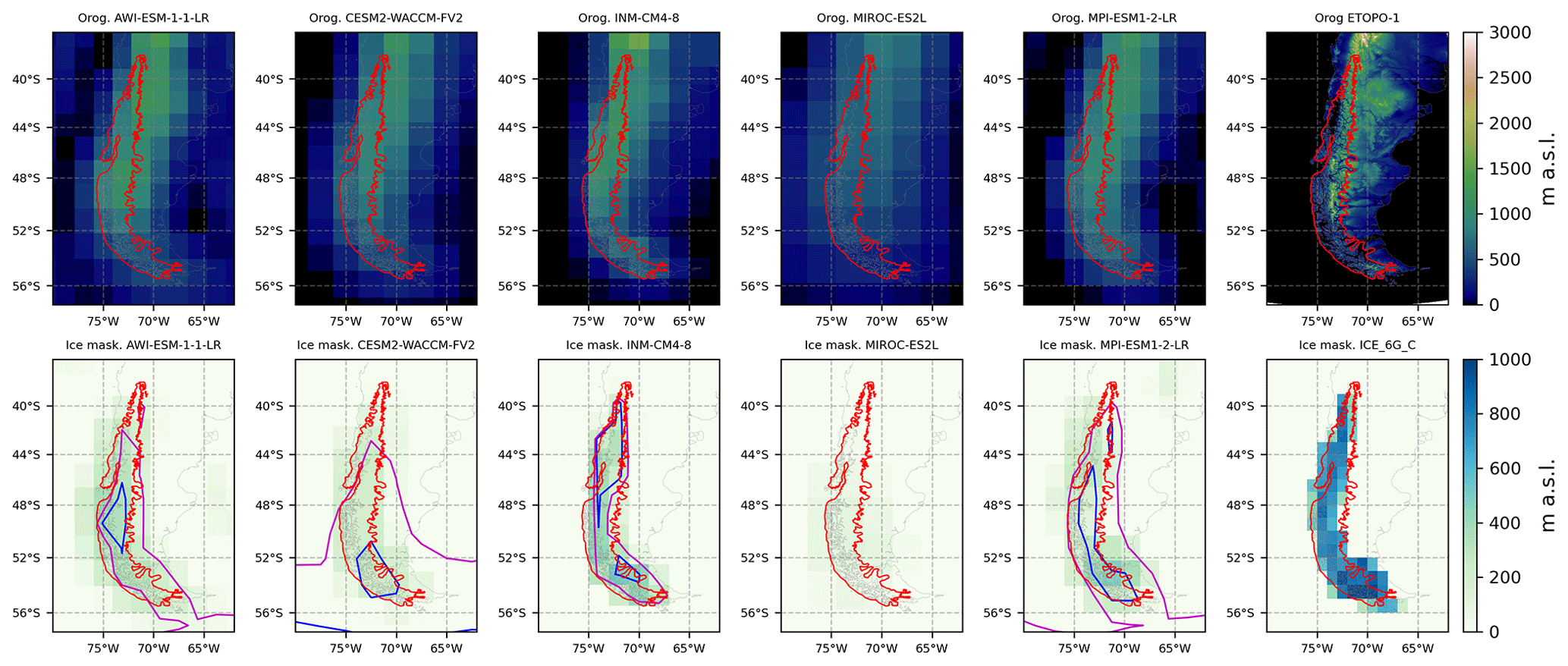
Figure 9 Prescribed topography (top) and ice thickness (bottom) of the PMIP4 models considered in this study. ETOPO1 (Amante and Eakins, 2009) and the ICE-6G_C reconstruction (Peltier et al., 2015) are included, are the ice sheet forcings in PMIP4. The red line shows the PIS extension for 20 ka (Davies et al., 2020). Blue and purple lines show the isotherm 0 °C for summer and the annual mean, respectively. Present-day ocean–continent limits are shown for interpretation.

Towards the southeastern sectors of the PIS, our findings reveal a consistent overestimation of ice sheet extents relative to the geological evidence. We partially attribute this to the discrepancies between the reconstructed PIS coverage and the prescribed topography in climate models. Prescribed ice sheets invade formerly ice-free territories, potentially inducing extra cooling and reduced ablation through a stronger albedo forcing. Inaccurate representation of the orographic effect on precipitation likely exacerbates mismatches between the modeled and reconstructed ice sheets as topographic forcing is flattened (Fig. 9), hindering the imposition of the rain shadow effect under coarse resolutions (Lofverstrom and Liakka, 2018; Bozkurt et al., 2019; Almazroui et al., 2021). This deficiency results in reduced precipitation on the windward side but much higher precipitation on the leeward side of the Andes, fostering PIS expansion beyond its geologically constrained eastern margin.

Studies of former Northern Hemisphere ice masses demonstrate that under the same orbital and greenhouse gas forcings, differences in the ice sheet boundary conditions yield significant impacts on the atmospheric circulation and temperature (Ullman et al., 2014; Löfverström et al., 2014; Bakker et al., 2020; Izumi et al., 2023). PMIP models generally capture temperature and precipitation conditions over South America during the LGM (Berman et al., 2016), yet they lack the resolution needed for detailed regional climate responses (Bozkurt et al., 2019). Thus, coarse resolution impedes modeling of Patagonia's narrow ice sheet. Higher climate model resolution is crucial for studying the influence of the Andean topography on past regional climate dynamics, which requires capturing the longitudinal gradient from the windward to the leeward side.

4.3 Glacial history of southern South America

A recent study has proposed the earlier LGM in Patagonia (Davies et al., 2020) and its consequent earlier deglaciation when compared with the Northern Hemisphere ice masses or Antarctica (Hughes et al., 2016; Batchelor et al., 2019; Gowan et al., 2021). However, the timing of the deglaciation along the PIS is not uniform (Darvill et al., 2015; Peltier et al., 2021; Lira et al., 2022; Hodgson et al., 2023; Peltier et al., 2023). In the northern part, the geochronological reconstruction proposed a relatively stable margin, with several re-advances, between the local LGM and the global LGM (Davies et al., 2020; Leger et al., 2021), with a rapid deglaciation that started at around 20 ka (Moreno et al., 2015; Davies et al., 2020). Conversely, in the southern counterpart, the deglaciation signal is more pronounced before the global LGM, suggesting that an earlier local LGM occurred between 30 and 45 ka (Kaplan et al., 2007; Darvill et al., 2015; Davies et al., 2020; Peltier et al., 2021).

As shown in our transient simulations in Sect. 3, the glacial index signal based on Antarctic ice cores drives a progressive growth of the modeled PIS through MIS3 to MIS2, reaching the maximum extension of the PIS towards the global LGM. In contrast, local offshore records seem to capture a signal that drives the PIS evolution in agreement with the geochronological reconstruction (Davies et al., 2020). On the one hand, ODP-1233, located near the coast of northern Patagonia, reproduces relatively stable climate conditions between 35 and 20 ka. On the other hand, MD07-3128 exhibits a negative trend during the same period, in correspondence with the reconstructed PIS behavior south of 52° S. The offshore record GeoB3327-5 suggests climate conditions that enable a more extensive ice sheet towards MIS3. However, the coarse sampling resolution and consequently poorly resolved history proposed by them should be taken into account. The extreme glacial index factor induces a large drop in the summer mean temperatures during the LGM. The precipitation shows a pronounced decrease in eastern Patagonia, even reaching zero in some places. This combination does not allow the ice sheet to over expand towards the east. The southernmost offshore records analyzed in this study, PS75/034-2, shows a similar behavior to the Antarctic ice core records. We hypothesize that this core captures a transitional signal between the climatic behavior of southern midlatitudes and the Antarctic cores.

4.4 Potential implications of dissimilar LGM timings in the Southern Hemisphere and Northern Hemisphere

The first challenge in this study is related to the assumption of climate and ice sheet equilibrium states during the global LGM. It is, however, an open question whether it is fair to generate PIS model reconstructions assuming that the ice sheet was in a steady state under the global LGM climate conditions and, if not, how to treat the lack of reliable climate forcing for the earlier periods of the last glacial cycle. The second challenge is related to the interpretation of major planetary drivers that enabled an asynchronous glacial response of the two hemispheres to changes in the orbital and greenhouse gas forcings (Doughty et al., 2015).

The geologically constrained gap between the local LGM timings in Patagonia and different parts of the Northern Hemisphere raises an important question about the drivers behind this asynchronicity. These drivers potentially involve climatic feedback mechanisms, hemispheric climate sensitivities to orbital and greenhouse gas forcings, and teleconnections between the two hemispheres (Darvill et al., 2016). The current evidence suggests that the local glacial peak in the southern Andes and Patagonia happened at about 35 ka (Zech et al., 2011; Davies et al., 2020), which is much earlier than the local LGM inferred for most of the paleo-ice sheets in the Northern Hemisphere. Aside from the Barents–Kara Ice Sheet and smaller glaciations in Asia, ice masses of the last glacial cycle attained their maximum extents and were driven towards maximum ice volumes during MIS2, at about 24–18 ka (Hughes et al., 2016; Patton et al., 2016; Gowan et al., 2021), by a strong cooling between 30 and 20 ka. According to the current state of knowledge, these massive ice sheets only began disintegrating at around 18 ka (Patton et al., 2017; Stokes, 2017; Gowan et al., 2021). The situation is different for the Southern Hemisphere. Due to a lack of large-scale paleo-ice sheets and scarce information about past fluctuations of the Antarctic Ice Sheet, it is necessary to look at the existing evidence for the advance and retreat history of smaller ice bodies to contextualize the situation in the Southern Hemisphere during the last glacial cycle. For example, records coming from an ice field located in the Southern Alps in New Zealand indicate that this ice mass reached its maximum extent at around 28 ka (Rother et al., 2014). According to recent studies, its growth towards 28 ka was influenced by a slight decrease in temperatures in the preceding 2 millennia (Darvill et al., 2016). The reconstructed air temperature cooling at this location is estimated to be between 6 and 6.5 °C below present, accompanied by a precipitation reduction of up to 25 % (Golledge et al., 2012b). During the period between 26 and 20 ka, this ice field is thought to have undergone a slow and continuous retreat, followed by a standstill at around 19 ka. This coincides with the time when most of the Northern Hemisphere ice sheets began retreating from their maximum positions due to slowly increasing solar radiation and activation of positive climate feedback mechanisms. Arguably, the Antarctic Ice Sheet seems to have been stable until about 18 ka, after which it experienced an increase in air temperatures synchronized with the increase in CO₂ concentrations (Parrenin et al., 2013; Brook and Buizert, 2018). This triggered the retreat of ice margins in Antarctica, New Zealand, and South America, where the PIS experienced an accelerated retreat starting from 18 ka (Davies et al., 2020). The current evidence of an early local LGM in Antarctica is inconclusive, partly due to an extreme sensitivity of the Antarctic Ice Sheet to the ocean forcing as opposed to the thermal atmospheric forcing playing the largest role in the deglaciation of formerly ice-sheet-covered areas (Golledge et al., 2012a). However, pieces of evidence from Patagonia and New Zealand suggest that the Southern Hemisphere might have responded very differently to the global cooling of the last glacial period compared to the Northern Hemisphere (Darvill et al., 2016; Shulmeister et al., 2019).

5 Conclusions

Using a combination of ice sheet modeling, paleoclimate model outputs, ice and sediment core records, and a recent geomorphological reconstruction, we explore the glacial history of the former ice sheet in Patagonia, with a focus on the timing of its maximum advance. As an initial assessment, we generate an ensemble of ice sheet model simulations driven by downscaled, steady-state paleoclimate reconstructions to get a first-order approximation of the extent the PIS could attain under peak global glacial conditions. By evaluating our ensemble against the PATICE reconstruction, we observe that most paleoclimate model products provide conditions that prevent the inception of the PIS at its northernmost margins while boosting an overestimated growth in the southeast, which is in alignment with earlier studies that implement different modeling choices. We perform a latitudinal analysis that reveals a narrow envelope of air temperature and precipitation rate pairs that foster a northern PIS growth in agreement with PATICE, while PMIP models typically showcase much warmer conditions. In contrast, cold-air summer temperatures in the southern PIS sector and the associated lack of surface ablation prompt an unchallenged advance under too-wet conditions that seem to ignore the Andean topographic barrier. By investigating the original representation of the region within the PMIP models we find that the topography is severely flattened along the Andes, which points to the possibility of a diminished rain shadow effect and subsequent overestimation of precipitation on the leeward side of the mountain range. Our findings highlight the need for a significantly higher climate model resolution to properly capture the complex longitudinal gradients of the Patagonian region.

To account for the seemingly asynchronous peak glacial advance of the PIS relative to the Northern Hemisphere ice sheets, we additionally produce an ensemble of transient ice sheet simulations driven by time-evolving climate conditions derived from a variety of ice core and offshore sediment records. Our results show that the climate forcing based on local sedimentary records is capable of driving a PIS advance that peaks around MIS3. In addition, we find latitudinal differences in the evolution of the PIS between this local peak and the global LGM: southern Patagonia and far-offshore records exhibit a warming trend during this period, whereas the northern sectors remain relatively stable. In a stark contrast, our experiments reveal that none of these patterns can be reproduced by ensemble members driven by climate conditions based on Antarctic records. This strong connection between the glacial history and regional circulation patterns in Patagonia suggests that the local paleoclimatic signal represents a key component in studies of the PIS evolution.