Large-ensemble simulations of the North American and Greenland ice sheets at the Last Glacial Maximum with a coupled atmospheric general circulation–ice sheet model

The Last Glacial Maximum (LGM) was characterised by huge ice sheets covering the Northern Hemisphere, especially over North America, and by its cold climate. Previous authors have performed numerical simulations of the LGM to better understand coupled climate–ice sheet systems. However, the results of such simulations are sensitive to many model parameters. Here, we perform a 200-member ensemble of simulations of the North American and Greenland ice sheets and climate of the LGM with a coupled ice sheet–atmosphere–slab ocean model (FAMOUS-BISICLES) to explore sensitivities of the coupled climate–ice system to 16 uncertain parameters. In the ensemble of simulations, the global mean surface temperature is primarily controlled by the combination of parameters in the large-scale condensation scheme and the cumulus convection scheme. In simulations with plausible LGM global mean surface temperatures, we find that the albedo parameters have only a small impact on the Greenland ice volume due to the limited area of surface ablation associated with the cold climate. Instead, the basal sliding law controls the ice volume by affecting ice transport from the interior to the margin. On the other hand, like the Greenland ice sheet in future climate change, the LGM North American ice sheet volume is controlled by parameters in the snow and ice albedo scheme. Few of our simulations produce an extensive North American ice sheet when the global temperature is above 12 °C. Based on constraints on the LGM global mean surface temperature, the ice volume and the southern extent of the North American ice sheet, we select 16 acceptable simulations. These simulations lack the southern extent of ice compared to reconstructions, but they show reasonable performance on the ice sheet configuration and ice streams facing Baffin Bay and the Arctic Ocean. The strong sensitivities of the North American ice sheet to albedo at the LGM may imply a potential constraint on the future Greenland ice sheet by constraining the albedo schemes.

1 Introduction

The rise in sea level predicted in the next several centuries associated with increasing greenhouse gases and global warming is one of the largest concerns of society and the climate science community. The most recent IPCC WG1 report projects a global mean sea level rise of more than 3 m under the high end SSP5-8.5 scenario for increase in radiative forcing in the next 300 years (IPCC, 2023). However, there are still large uncertainties in projections of sea level rise with the possibility of a much larger magnitude (Edwards et al., 2021). This large uncertainty in the projection of sea level rise reflects the present limited state of knowledge of several important processes, such as non-linear behaviours in the ice sheet system (e.g. Gregoire et al., 2012; Abe-Ouchi et al., 2013; Golledge et al., 2019) and interactions between the climate and the ice sheets, which are expressed in coupled climate–ice sheet models (e.g. Deconto and Pollard, 2016; Golledge et al., 2019; Gregory et al., 2020; Smith et al., 2021a). This uncertainty shows the importance of improving our understanding of the coupled ice sheet–climate system and refining numerical models used for the future projection of climate and sea level rise.

One method of evaluating coupled climate–ice sheet models and improving understanding of the coupled climate–ice sheet system is to simulate conditions of past periods. In this regard, the Last Glacial Maximum (LGM), which corresponds to approximately 21 000 years before present (ka BP; Clark et al., 2009; Kageyama et al., 2021), is useful since both climate conditions and the ice sheet configurations are relatively well documented compared to previous periods of glaciation (Tarasov et al., 2012; Kageyama et al., 2021). It has been suggested that the LGM could be used to constrain climate sensitivity (Tierney et al., 2020), cloud processes (Zhu et al., 2022) and deep-ocean circulation (Sherriff-Tadano et al., 2023), implying that understanding this period has the potential to help constrain climate and ice sheet models and future sea level projections. During this period, weaker summer insolation and lower concentrations of greenhouse gases caused the climate to be colder, allowing ice sheets to expand over North America and northern Europe. As a result, the global climate was colder by 1.7 to 8.3 °C (Holden et al., 2010; Schmittner et al., 2011, Tierney et al., 2020; Paul et al., 2021) and global mean sea level was approximately 120 m lower compared to modern (Clark et al., 2009; Gowan et al., 2021). The mass of the Greenland ice sheet is thought to have been larger by approximately by 2 to 5 m sea level equivalent (SLE) at the LGM (Clark and Mix, 2002; Lecavalier et al., 2014; Bradley et al., 2018; Tabone et al., 2018), while the mass of the Antarctic ice sheet is thought to have been larger by 5.6 to 14.3 m SLE (e.g. Briggs et al., 2014). The Eurasian ice sheet is thought to have attained a volume of 24 m SLE (Hughes et al., 2016), but by far the largest part of the 120 m SLE is attributed to the growth of the North American ice sheet (at least 60 m SLE, e.g. Abe-Ouchi et al., 2015). The position of the margin of the North American ice sheet is constrained reasonably well by geological evidence, and this line of evidence is often used to validate the performance of ice sheet models (e.g. Dyke et al., 2002; Clark et al., 2009).

Studies that simulate LGM climate and ice sheets have primarily treated these components independently using separate numerical models. To investigate the effect of ice sheets on climate, following Manabe and Broccoli (1985), many simulations have been performed and compared, including in studies contributed to the long-running Paleoclimate Model Intercomparison Project (PMIP, Braconnot et al., 2007; 2012, Ivanovic et al., 2016; Kageyama et al., 2017). The ice sheet configuration was specified as a boundary condition in these simulations, which show the important role of the ice sheets on glacial climate, affecting surface temperature, precipitation, and atmospheric and oceanic circulation (Smith and Gregory, 2012; Klockmann et al., 2016; Gregoire et al., 2018; Ivanovic et al., 2018; Sherriff-Tadano et al., 2021). To investigate the effect of climate on ice sheets, simulations of the LGM ice sheets have been performed with ice sheet models, either as full glacial cycle experiments (e.g. Abe-Ouchi et al., 2007) or equilibrium LGM experiments (e.g. Alder and Hostetler, 2019). In these experiments, the ice sheet models were forced with climatic conditions based on outputs from general circulation models (Gregoire et al., 2012; Abe-Ouchi et al., 2013; Alder and Hostetler, 2019; Niu et al., 2019; Blasco et al., 2021). They showed the critical effects of uncertain climatic conditions and albedo in causing a large diversity in the simulated ice sheet configuration (Abe-Ouchi et al., 2007; Alder and Hostetler, 2019; Niu et al., 2019; Blasco et al., 2021) together with uncertainties in basal sliding law (Gandy et al., 2019). These studies highlighted the strong interaction of climate and ice sheets and the importance of performing simulations with coupled climate–ice sheet models to better understand the coupled system.

Recent efforts in the modelling community toward developing complex coupled climate–ice sheet models (e.g. Gregory et al., 2012; Ziemen et al., 2014; Roche et al., 2014; Smith et al., 2021b) mean that higher-complexity coupled climate–ice simulations of the glacial period than have previously been possible may now be performed. Gregory et al. (2012) performed simulations of an ice sheet inception over North America with the coupled climate–ice sheet model FAMOUS-Glimmer. They showed the role of the albedo on the magnitude and speed of the inception. Ziemen et al. (2014) performed simulations of the ice sheet–atmosphere–ocean system with a more complex coupled ice sheet–climate model. Their simulation reproduced the climate and the ice sheets of the LGM reasonably well, while the southern extent of the North American ice sheet was somewhat smaller compared to reconstructions. This is partly due to the relatively coarse resolution of the atmospheric model (Ziemen et al., 2014), which means their model underestimated the stationary wave effect that cools the southern extent of the North American ice sheet and hence underestimates the ice area in that region (Roe and Lindzen, 2001; Abe-Ouchi et al., 2007). Lofverstrom et al. (2015) performed simulations of the North American ice sheet and climate with a coupled atmosphere–ice sheet–slab ocean model in an idealised framework and showed the importance of interactions between atmospheric circulation, the Rocky Mountains and the ice sheet in shaping the ice sheet's zonally asymmetric features. Willeit and Ganopolski (2018) presented simulations of the last glacial cycle with an ice sheet model coupled to an Earth system model of intermediate complexity and discussed the role of the darkening effect of snow. Quiquet et al. (2021) performed simulations of the ice sheets and climate of the LGM and the last deglaciation with a coupled climate–ice sheet model. They managed to reproduce the overall characteristics of the evolution of climate and ice sheets and showed the effects of modulations in the oceanic circulation.

These previous studies provide very useful insight into the physical interactions within the coupled system, but the inherent uncertainty and sensitivity in the simulations to the selection of model inputs (including physical parameterisations) are not tested in any of these studies because they each use a single version of a given model.

Perturbed parameter ensembles of simulations are a powerful way to estimate uncertainties originating from particular parameter values in a single model (Murphy et al., 2004; Sanderson, 2011; Shiogama et al., 2012). For example, Rougier et al. (2009) analysed results from an ensemble performed under modern and future climate conditions with a coupled atmosphere–slab ocean general circulation model (HadSM3) and showed the critical role of entrainment rate in the cumulus cloud scheme and its interaction with a large-scale condensation scheme on global climate. Gregoire et al. (2011) performed an ensemble of simulations with a coupled atmosphere–ocean general circulation model, FAMOUS, and found that the mid-latitude cloud parameters and sea ice albedo exert an important influence on global cooling at the LGM. Furthermore, they used their results to identify combinations of parameter values that optimise model skill in simulating both the pre-industrial and LGM, thus improving model flexibility. Gandy et al. (2023) recently performed ensemble simulations of the North American ice sheet and climate with a coupled atmosphere–ice sheet model FAMOUS-Ice (Smith et al., 2021a). They showed the importance of ice and snow albedo in building the ice sheet due to strong summer insolation at the southern margin of the North American ice sheet. In this study, however, the sea surface temperature and the global temperature were fixed. As a result, the role of clouds on the climate and the effects of global mean surface temperature (GMST) on the ice sheet volume could not be examined.

Here, we perform a large ensemble of simulations of the North American and Greenland ice sheets and climate of the LGM with a version of the FAMOUS-Ice coupled atmosphere–ice sheet model, including a more sophisticated ice sheet model, BISICLES (Method, e.g. Smith et al., 2021b). With this ensemble, we estimate the impact of uncertainty in the choice of parameter values implemented in the atmosphere and ice sheet components of the model, and we test the ability of the model to simulate ice sheets and climates very different from today. The results are evaluated against the LGM GMST, ice volume and southern extent of the North American ice sheet. Through these experiments, we aim to address the following questions.

• How do uncertain parameters affect the climate and ice sheets at the LGM?

• Is there a difference in important parameters between the North American and Greenland ice sheets?

• How well are the ice sheets simulated in this experiment, e.g. in terms of North American ice sheet volume, the southern extent of the North American ice sheet and the position of the ice streams?

The remainder of the paper is structured as follows. Section 2 gives a description of the model, the experimental design and the integration procedure. Section 3 reports on the results of the large ensemble. Section 4 discusses the results and the effect of biases in the model. Lastly, Sect. 5 gives the conclusions.

2 Method

2.1 Model

Our simulations of the climate and ice sheets are performed with the coupled atmosphere–ice sheet–slab ocean model FAMOUS-Ice (Smith et al., 2021a; Gregory et al., 2020). FAMOUS is a low-resolution version of the atmosphere–ocean general circulation model (AOGCM) HadCM3; the horizontal resolution is 7.5° in longitude and 5° in latitude (Smith et al., 2008). Due to the lower resolution, FAMOUS runs 10 times faster compared to HadCM3 while retaining a reasonable performance for the modern and the LGM climates (Smith et al., 2008; Smith and Gregory, 2012). Benefitting from much cheaper computational cost, it is feasible to run multi-millennial simulations (Smith and Gregory, 2012; Gregory et al., 2020) and large ensembles (Gregoire et al., 2011), as required to meet our objectives.

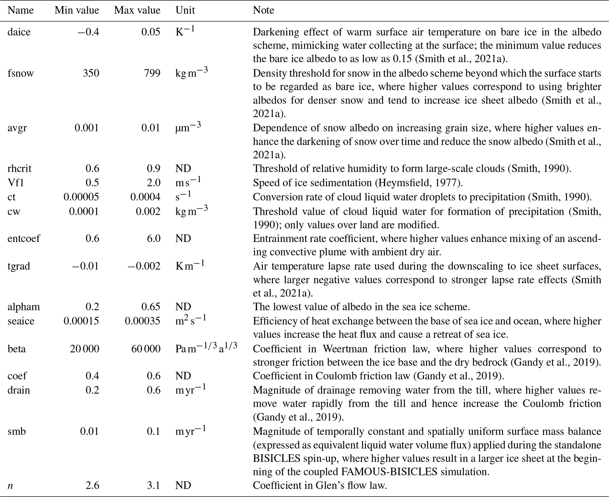
Table 1 Summary of parameters modified in the ensemble simulations. ND stands for non-dimensional.

The latest version of FAMOUS (FAMOUS-Ice, Smith et al., 2021a) incorporates a downscaling scheme for the calculation of the surface mass balance (SMB) over ice sheets. In the downscaling scheme, 10 additional vertical tiles are added to better represent the elevation dependence of surface temperature and downward longwave radiation, following the method first used in Vizcaino et al. (2013). The downscaled temperature and longwave radiation are then utilised with downward shortwave radiation to calculate the SMB based on a surface energy budget and a multi-layer snow scheme, together with precipitation from the original FAMOUS grid. The model also incorporates an updated snow and ice albedo scheme, which accounts for albedo changes associated with modifications in surface air temperature (daice), grain size (avgr) and density of the snow (fsnow) (Smith et al., 2021a, Table 1). As a result, the atmospheric model reproduces the general pattern of SMB over the modern Greenland ice sheet reasonably well (van de Wal et al., 2012; Smith et al., 2021a) with some overestimation of the elevation of equilibrium-line altitude (ELA; Smith et al., 2021a; see also Sect. 4.3).

Previous work with FAMOUS-Ice used prescribed climatological sea surface temperatures (SSTs) and sea ice instead of an interactive ocean model (Gregory et al., 2020; Smith et al., 2021a; Gandy et al., 2023). In the present study, we use a slab ocean model with the same horizontal resolution as the atmosphere. Inclusion of a slab ocean model allows the local and global SST and sea ice to vary in response to changes in climate, which in our experiments are caused by modifications in parameters and the advance and retreat of ice sheets. In the slab ocean model, sea ice is advected by the climatological monthly surface seawater velocity of the HadCM3 pre-industrial control experiment, with sea ice convergence prevented when the local thickness exceeds 4.0 m. The local thickness of sea ice evolves due to snowfall, sublimation and melting at the surface and melting and freezing at the base in response to heat exchange with the slab ocean. The SST is the temperature of a layer of water 50 m thick and evolves in response to surface energy exchange with the atmosphere and heat transport within the slab ocean. Since the slab ocean does not simulate ocean dynamics, climatological heat transport is prescribed within it as a monthly climatological field of heat convergence. The heat convergence field is obtained from a calibration experiment (Sect. 2.2) in which the model calculates the heat flux necessary to maintain a reference climatological state of SST and sea ice.

The slab ocean model is essentially the same as described by Williams et al. (2001), where it is used with the HadCM3 AOGCM, but the present study is the first to use it with the atmosphere resolution of FAMOUS. For this configuration, grid boxes that are partly land and partly sea were implemented in the slab ocean, as in the AOGCM. In order to prevent unstable surface temperature feedbacks in coastal grid boxes with small sea fraction, we found that horizontal diffusion of heat in the slab ocean was needed (diffusivity 10 000 m² s⁻¹); unlike the prescribed heat convergence, diffusive heat divergence responds to the time-dependent slab temperature gradient and thus dissipates local anomalies, but usually it is much smaller than the heat convergence. In order to prevent local build-up of excessively thick coastal sea ice, we allow horizontal diffusion of sea ice thickness (diffusivity 5000 m² s⁻¹) when the local thickness exceeds 4.0 m. To improve the reproduction of the reference sea ice climatology, we adjusted the coefficients for sea ice basal melting.

Instead of the Glimmer ice sheet model that was used in the previous studies of FAMOUS-Ice (Gregory et al., 2020; Smith et al., 2021a; Gandy et al., 2023), we use the more complex and computationally demanding BISICLES model (Cornford et al., 2013) for the ice sheet component of FAMOUS-Ice (hereafter referred to as FAMOUS-BISICLES). BISICLES is a vertically integrated ice sheet model, which has been mainly used for simulations of modern and future Greenland (Lee et al., 2015; Smith et al., 2021b) and Antarctica (Martin et al., 2019; Smith et al., 2021b) and has recently been used to simulate past ice sheets over North America (Matero et al., 2020) and northern Europe (Gandy et al., 2018, 2019, 2021). Whereas Glimmer uses the shallow ice approximation, BISICLES applies a L1L2 approximation, which allows more flexibility in sliding and flowing of the ice sheet, especially at the ice shelf area (Cornford et al., 2013). In addition, the model is capable of changing spatial resolution according to the flow regime of the ice. In this study, a horizontal base resolution of 32 km is chosen, with refinement to 16 km at ice sheet margins. The choice of the resolution was made based on practical reasons regarding the computational expense. We show that this resolution is adequate for simulating large-scale glaciers in the northern area of the North American ice sheet (see Sect. 4.2).

We utilise a basal drag scheme introduced by Gandy et al. (2019), which explicitly expresses the thermodynamic interaction of the ice sheets and the underlying till. This scheme combines the Coulomb friction law and Weertman friction law depending on the water pressure in the bedrock sediment (Tsai et al., 2015). The basal drag follows the Weertman law under cold ice basal temperature and dry bedrock sediment. Under warm ice basal temperature and wet bedrock sediment, the basal drag follows the Coulomb friction law. Depending on the depth of till water in the sediment, the friction of ice and bedrock changes. The depth of the till water is controlled by the balance of basal melting of the ice sheet and a parameter (drain) that controls the vertical till-stored drainage rate. Using this basal scheme in BISICLES simulations, Gandy et al. (2019) reproduced the features of known ice streams in the LGM British ice sheet.

Changes in ice sheet geometry and the subsequent redistribution of the Earth's surface mass load result in deformation of the Earth's topography through a series of interconnected processes known as glacial isostatic adjustment (GIA). An important impact of GIA for the purpose of ice sheet modelling is the subsidence of the bedrock topography beneath an ice sheet. The rate of the solid Earth response towards isostatic equilibrium, which can range from centuries to millions of years, is viscoelastic in nature as a result of the rheological structure of the Earth and specific pattern of ice loading. In order to simulate the first-order effects of GIA on bedrock topography, we couple the ice sheet model to a simple elastic lithosphere relaxing asthenosphere (ELRA) model that approximates this response by assuming a fully elastic lithosphere above a uniformly viscous asthenosphere (Kachuck et al., 2020). A relaxation time of 3000 years is applied in this model based on previous studies (Pollard and Deconto, 2012).

In running FAMOUS-BISICLES, a 10-times acceleration factor is applied to the ice sheet model to save computational cost (Gregory et al., 2012; Ziemen et al., 2014). In this method, the ice sheet model is integrated for 10 years for every 1 year of climate simulation by FAMOUS. Gregory et al. (2012) and Gregory et al. (2020) show that 10-times acceleration has a small to negligible impact on the simulated ice sheet evolution in FAMOUS, supporting the use of this technique.

2.2 Experimental design

Our experiments mainly follow the protocol of PMIP4 LGM simulations (Kageyama et al., 2017, 2021), which specifies the insolation, atmospheric concentration of greenhouse gases (CO₂ = 190 ppm, CH₄ = 375 ppb, NO₂ = 200 ppb, all by volume) and configurations of continental ice sheets. The Eurasian and Antarctic ice sheets are fixed to the reconstruction of GLAC-1D (Tarasov et al., 2012) in our setup, while the North American and Greenland ice sheets are simulated with BISICLES. While the protocol specifies the insolation forcing of 21 ka BP, here we use the insolation of 23 ka since the ice sheet at the LGM is likely still adjusting to earlier forcing (Abe-Ouchi et al., 2013).

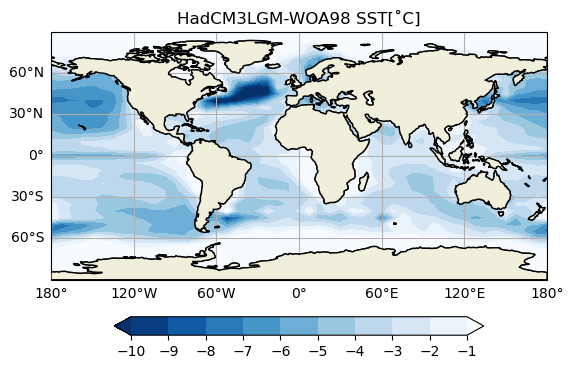
Figure 1 Annual mean sea surface temperature anomaly fields (K, colour) between a HadCM3 LGM simulation and modern observation World Ocean Atlas 1998 (Levitus and US National Oceanographic Data Center, 2012). The sea surface temperature field from HadCM3 is used as the target sea surface condition for our prescribed slab ocean setup.

For calibrating the slab ocean heat convergence (Sect. 2.1), we use the SST and sea ice climatology from a previous LGM simulation performed with HadCM3, shown in Fig. 1 (Izumi et al., 2023). Their simulated GMST exhibits a cold LGM climate, having a global cooling of 6.5 K. This value is similar to Tierney et al. (2020), who estimate 6.5 to 5.7 K. For simplicity of design and clarity of interpretation, the oceanic heat flux is fixed among all the ensemble simulations, thus assuming no changes in the oceanic heat transport in response to the different parameter values in each member.

We perform 200-member ensemble simulations by varying 16 parameter values associated with climate and ice dynamics, as summarised in Table 1, using a Latin hypercube sampling method (Williamson, 2015), assuming a uniform value probability across each parameter range, in order to explore the full range of the 16-dimensional parameter space. The Latin hypercube sampling technique is useful as it allows exploration of all the uncertain parameter spaces in an efficient way. While some cancellations among parameters can cause lower correlation values between inputs and outputs, the method also provides quantitative insights on the complex interactions among different parameters (e.g. Figs. 6 and S7 in the Supplement in this study).

The choice and the range of the parameter values in FAMOUS are modified following Gregoire et al. (2012) and Gandy et al. (2023). In BISICLES, the range of sliding law parameters are modified following sensitivity experiments of Gandy et al. (2019). For drain, which specifies the vertical till-stored drainage rate, the value is very uncertain, and hence we varied it to ensure that the till of the interior of the ice sheet remains dry. Much lower values for drain, as used in Gandy et al. (2019) in their simulation of the much smaller British–Irish ice sheet, result in unphysically wet basal conditions and fast sliding in our simulations, so we used a higher range. For n, which specifies the coefficient in Glen's flow law, the range is selected in a practical way: applying a high value increases the calculation time by more than 10 times due to very large ice velocities and the resulting refinement in several locations. Hence, the range of n is necessarily capped for its upper limit at 3.1, where our technical tests indicated that the simulations will most likely complete within a feasible run length (2 months of wall-clock time). During the ice sheet spin-up phase (see Sect. 2.3), we specify a constant SMB. The value of this “smb” is varied across the ensemble so that the ice volume at the initiation of FAMOUS-BISICLES coupling has a spread of 25 m SLE, which is similar to the uncertainty in the global ice volume estimates at the LGM (e.g. Abe-Ouchi et al., 2015). For simplicity, we apply spatially uniform basal heat fluxes of 158 mW m⁻² and 100 W m⁻² under the grounded and floating ice, respectively, without testing other values. However, these choices need to be reassessed in the future because the basal heat flux over both the continent (e.g. Margold et al., 2018) and the ocean can vary spatially.

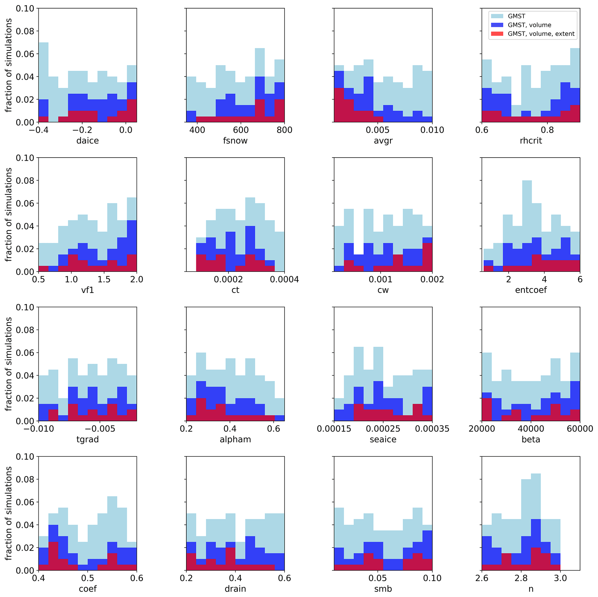
Figure 2 Fraction of the 200 simulations that satisfy the constraints as a function of each of the parameters. A total of 200 members are uniformly distributed in each parameter range based on the Latin hypercube sampling method (approximately 20 simulations per parameter bin). Light blue shows ensemble members satisfying the global mean surface temperature (GMST) constraint, dark blue shows ensemble members satisfying both the GMST and the North American ice volume constraints, and red shows ensemble members satisfying the southern North American ice sheet margin constraints in addition to the GMST and the North American ice volume constraints.

2.3 Integration procedure

Model simulations are all initiated from a static, isothermal (ice temperature 253 K) ice sheet and bedrock topography of 21 ka BP of GLAC-1D (Fig. 3a and f, Tarasov et al., 2012). The simulations have two phases. First, there is an initial spin-up of 5000 ice sheet years with standalone BISICLES, where the ice sheet model parameter values are chosen according to the ensemble Latin hypercube sampling, but the associated climate parameter values are not used because there is no climate model. In place of the climate model, a constant-in-time surface mass balance (smb, Table 1) and atmospheric surface temperature of 253 K are applied uniformly over the ice. Note that the ice temperature is allowed to evolve in the simulation. The smb value is varied across the ensemble to produce a variety of total ice volumes (Fig. S1) because total ice volume is highly uncertain in reconstructions and could be important given the dependence of ice sheet simulation on initial conditions (Abe-Ouchi et al., 2013). The spin-up phase also gives the ice sheet model physics time to adjust from the prescribed initial condition, i.e. it allows BISICLES to smooth out the blocky surface of the ice sheet reconstruction, providing some stability to the simulations when they are subsequently coupled to the climate (FAMOUS) in the second phase. By the end of the spin-up phase, 200 unique ice sheets have been modelled, providing the starting condition for simulations with BISICLES coupled to FAMOUS in the second phase. In FAMOUS-BISICLES, smb is redundant and the climate parameters chosen by Latin hypercube are used in FAMOUS, with the same ice sheet parameter combinations as in the spin-up phase. In the second phase, the simulations run for 5000 ice sheet (500 climate) years, which is insufficient to reach a quasi-equilibrium state but sufficiently long to see the effects of important parameters on the climate and ice sheets. For some of the best-performing simulations, the integration is extended for another 5000 ice years, during which the configuration of the ice sheet shows only modest further changes (Fig. S2).

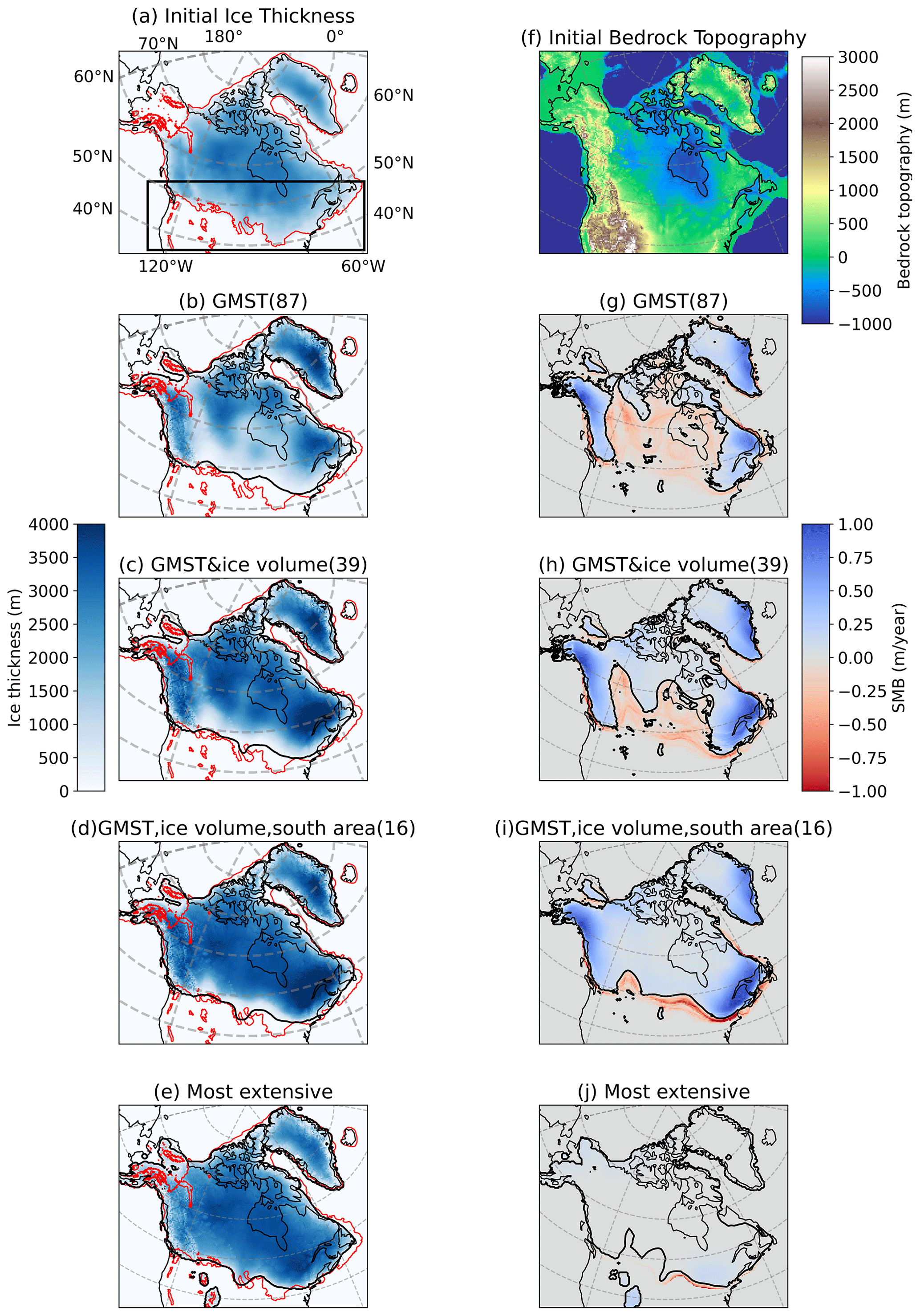
Figure 3 Spatial maps of the initial condition for the ice sheet model and results from the FAMOUS-BISICLES ensemble after 5000 ice sheet years. (a) Ice topography (m) and (f) bedrock topography (m) from Tarasov et al. (2012). (b–e, top) Spatial maps of ice thickness (m) and (g-j, bottom) surface mass balance (SMB) (m yr⁻¹) from ensemble means. (b, g) A total of 87 members satisfying the global mean surface temperature (GMST) constraint, (c, h) 39 members satisfying both GMST and ice volume constraints, (d, i) 16 members having the largest southern extent of North American ice sheet that satisfies GMST and volume constraints, and (e, j) the member with most extensive southern ice area in the ensemble simulations. The thin black contour corresponds to the modern coastline, whereas the thick black contour in (g–j) corresponds to the zero line of SMB. Red contours in (a–e) correspond to the ice extent of Dalton et al. (2020). Black contours in (b–e) correspond to the ice extent of the ensemble mean defined as 100 m ice thickness. The black rectangle in (a) shows the region where the southern extent of the North American ice sheet is calculated (e.g. Fig. 11).

2.4 Constraints

Three metrics are used to evaluate the large-scale feature of the ensemble simulations. These are the annual mean LGM GMST, the ice volume of the North American ice sheet and the southern extent of the North American ice sheet.

Figure 4 Evolution of GMST in the FAMOUS-BISICLES ensemble of simulations. Each grey line represents one ensemble member. Results from the first 300 ice years (30 climate years) are shown. The uncertainties in GMST are shaded blue (3 standard deviations for light blue and 2 standard deviations for dark blue). Histograms on the right show the number of simulations in each temperature bin.

For the global temperature, we create our LGM constraint by adding estimates of the LGM global cooling to the pre-industrial GMST of 13.7 °C (1880–1900; NOAA National Centers for Environmental Information, 2023) with an uncertainty of ± 0.1 °C (1 standard deviation of global temperature during this period). According to previous studies, the LGM global cooling relative to the pre-industrial period has a range of −1.7 to −8.3 °C (e.g. −1.7 to −3.7 °C with a probability of 90 % in Schmittner et al. (2011) and −4.6 to −8.3 °C with a probability of 90 % in Holden et al. (2010); see Fig. 4a in Tierney et al., 2020). To objectively cover all the possibilities, we take into account all of these studies to define our range of plausible LGM GMST. Assuming the LGM cooling is normally distributed, this gives a mean cooling of 5 °C ± 3.3 °C with a probability of 90 % (1 standard deviation is ± 2.0 °C). Combining the uncertainties associated with the pre-industrial GMST and the LGM global cooling gives 1 standard deviation of the uncertainty of

$$\begin{array}{}\text{(1)}& \sqrt{(\mathrm{0.1}{)}^{\mathrm{2}}+(\mathrm{2.0}{)}^{\mathrm{2}}}=\pm \mathrm{2.0}\mathrm{°}\mathrm{C},\end{array}$$

in the actual LGM GMST (66 % probability). To be conservative and take into account model uncertainty, we apply 3 standard deviations (± 6.0 °C) as the uncertainty ranges. This gives an actual LGM GMST of approximately 2.7 to 14.7 °C (8.7 °C ± 6.0 °C), with a probability of at least 99 % (Pukelsheim, 1994).

For the ice volume constraint, previous studies have suggested that the volume of the North American ice sheet was likely to be larger than 70 m sea level equivalent (cf. Abe-Ouchi et al., 2015). To account for model uncertainty and to be conservative, we apply a minimum reasonable North American ice volume of 60 m SLE as a constraint. Applying an upper ice volume limit may also be important in constraining the parameter space. However, in general, equilibrium LGM simulations tend to overestimate the ice volume if once the simulation has a net positive SMB (e.g. Alder and Hostetler, 2019). In this regard, setting an upper limit can be tricky, and it therefore needs to be examined in a different experimental set-up.

The southern extent of the North American ice sheet is used to select the best-performing simulations, rather than as a strict constraint, because all ensemble members show a smaller southern area of the ice sheet than reconstructions (see Sect. 4.1). Areas of grid cells covered by the ice sheet in the box shown in Fig. 3a are calculated. This area corresponds to the south of Hudson Bay. Simulations with the southern area covering 60 % of the reconstructed area (Dalton et al., 2020) are considered to satisfy our constraint.

In the end, 16 simulations simultaneously satisfy our constraints on temperature, ice volume and extent.

Figure 5 Relationship between GMST averaged over ice years 200–290 (climate years 20–29) and each parameter value. Correlation values are displayed above each panel. The uncertainties in GMST are shaded blue (3 standard deviations for light blue and 2 standard deviations for dark blue).

3 Results

3.1 Response of the GMST

Figure 4 summarises the temporal evolution of annual mean GMST in the ensemble of simulations. After the first 300 ice sheet years, climates reach a quasi-equilibrium. The results show a wide variety of simulated global temperatures, ranging from −10 to 40 °C. Such a wide range is frequently observed under parameter ensemble simulations (e.g. Joshi et al., 2010; Gregoire et al., 2011). The diverse response of GMST is largely explained by two parameters in the cloud schemes; ct in the large-scale condensation scheme and entcoef in the cumulus convection scheme (Fig. 5). The correlation coefficients of these parameters with the global temperature at ice years 200–290 are 0.622 for ct and −0.574 for entcoef, respectively. In contrast, other parameters appear to have a smaller effect, according to the correlation analysis (Fig. 5). For the sea ice albedo, this relatively muted sensitivity may be related to the use of a slab ocean model, which underestimates the strong interactions between sea ice and oceanic heat transport over the Southern Ocean that amplifies the surface cooling at high latitudes (Ogura et al., 2004; Zhu and Poulsen, 2021). Including a dynamical ocean may increase the importance of sea ice albedo on the GMST, as shown by Gregoire et al. (2011).

Roles of ct and entcoef in governing GMST are further explored by means of a pair plot in Fig. 6, which compares the relationship of these two parameters to GMST. The results show a positive correlation between global-scale warming and ct, which is associated with an increase in precipitation efficiency, reducing the life cycle of mid-latitude clouds, causing a decrease in the cloud cover and a decrease in the planetary albedo. As a result, more shortwave radiation is absorbed and the planet warms (Joshi et al., 2010; Sherriff-Tadano et al., 2023). Conversely, global-scale warming occurs with decreasing entcoef (Fig. 6), as the entrainment rate of ambient dry air in the tropics reduces and the vertical transport of moisture to the high troposphere and lower stratosphere enhances. The planet then warms up due to the strong greenhouse gas effect of the water vapour (Joshi et al., 2010). Similar responses are observed in Joshi et al. (2010), who performed ensemble simulations under modern and future climates and showed that low values of entcoef were unrealistic based on the amount of water vapour in the lower stratosphere. Consistently, ensemble members with very low values of entcoef are more likely to be ruled out for producing implausible GMSTs, depending on the effect of the combinations of the other parameters (Fig. 6). For ensemble members satisfying the temperature constraint (black-outlined coloured dots in Fig. 6), the overall cooling and warming effects of ct and entcoef are largely cancelled out by each other.

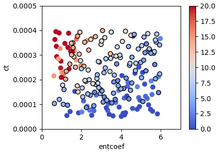
Figure 6 Pair plot analysis exploring the combined effects of ct (precipitation efficiency in the large-scale condensation scheme) and entcoef (entrainment rate in the cumulus convection scheme) on GMST (colours, °C). Filled circles outlined in black are those satisfying the temperature evaluation criterion.

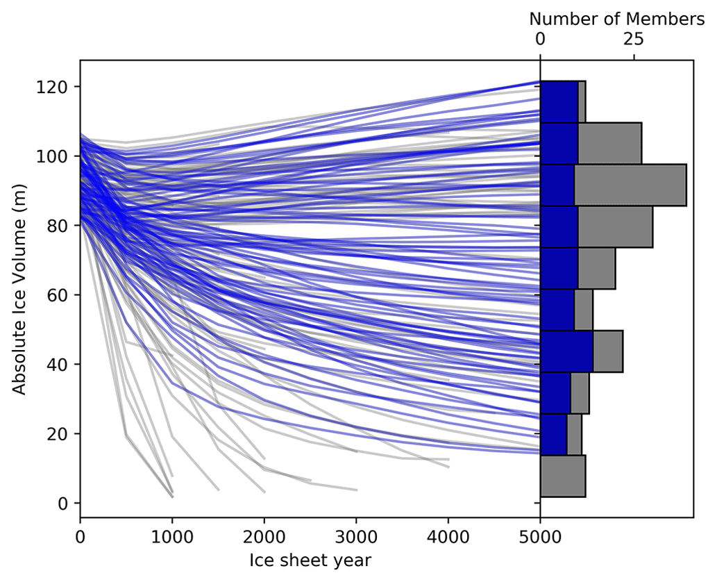
Figure 7 Evolution of the North American and Greenland combined SLE ice volume in the FAMOUS-BISICLES LGM ensemble. Note that the modern ice volume of 7.3 m SLE on Greenland is included; the ice volume is not the difference between LGM and present. Each grey line represents one ensemble member. Blue lines are the members satisfying our chosen GMST evaluation criteria. Histograms on the right show the number of simulations in each temperature bin, with grey indicating all members and blue members satisfying the GMST constraint.

3.2 Response of the North American ice sheet

Similar to the diversity in simulated GMST, the evolution of the ice sheet after the coupling to FAMOUS shows a wide range of responses (Fig. 7). Starting from combined ice sheet volumes of 80 to 105 m SLE (sum of North American and Greenland ice sheets), the ensemble members produce combined ice volumes between 0 and 120 m SLE at the end of the 5000-ice-year integration. In some simulations, even the Greenland ice sheet disappears completely associated with the very high global temperature (Fig. 4). Note that some simulations with high n values or very warm climates (that cause all of the ice to rapidly disappear) crash during the integration. In total, 139 members (∼ 70 % of the ensemble) complete the entire 5000 ice years. A total of 87 members satisfy the global temperature constraint (Figs. 5 and 6), and 39 members also satisfy the North American ice volume constraint of at least 60 m SLE. The additional constraint on the southern extent of the North American ice sheet selects the 16 best-performing simulations (Fig. 2).

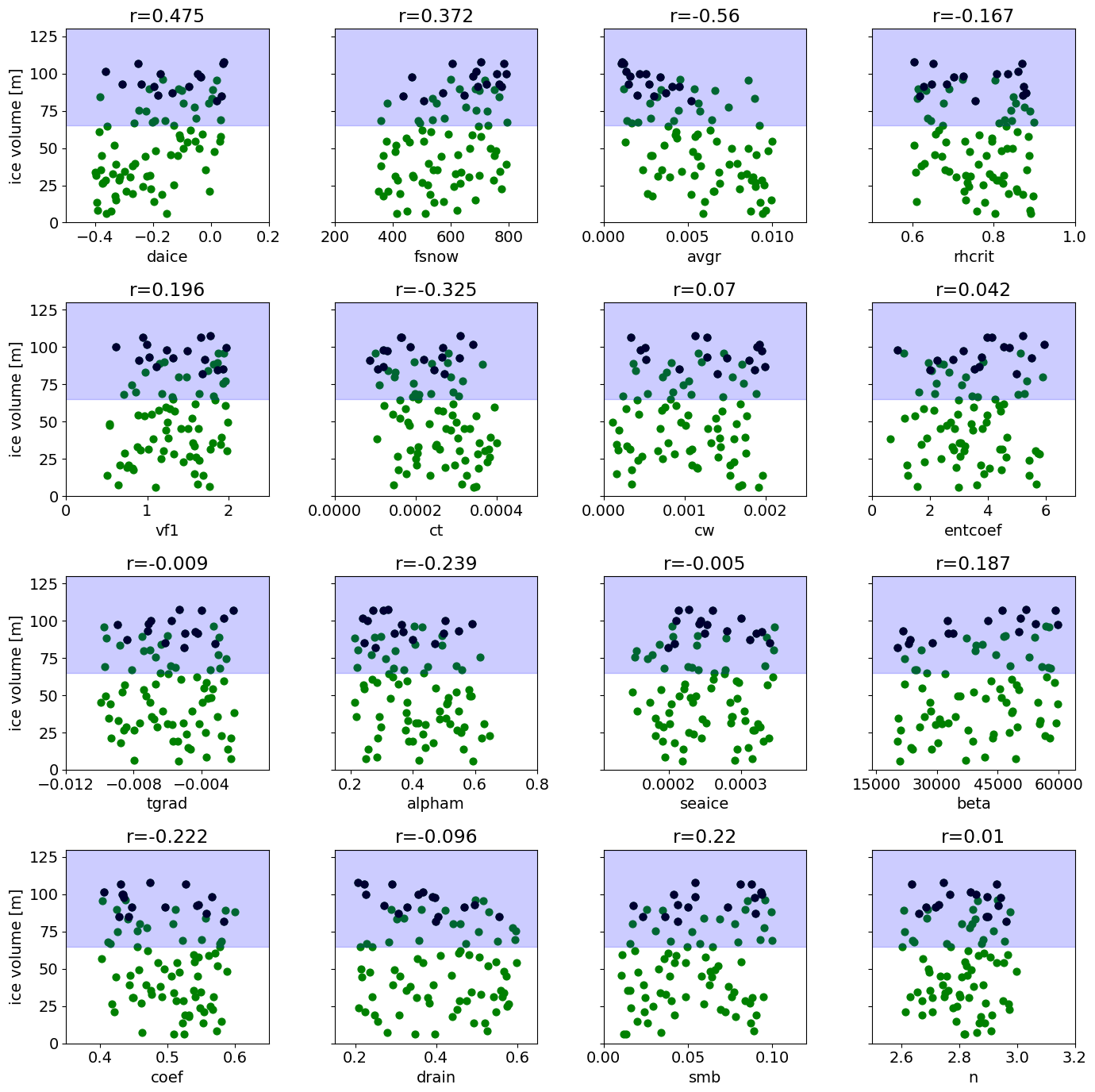
Figure 8 Relationship between North American ice volume at 5000 ice years in FAMOUS-BISICLES and each perturbed parameter. Only those ensemble members that satisfy the GMST constraint are used. Correlation values are displayed above each panel. Black dots correspond to the best 16 members. The uncertainties in the North American ice volume constraint are shaded blue.

To explore which parameters are causing the variety of outcomes for the simulated North American ice volume, scatter plot and correlation analyses are performed (Fig. 8). Here, the ensemble members that both satisfy the GMST constraint and have completed 5000 ice years are used (87 members). The analysis shows important impacts from parameters in our ice sheet surface albedo scheme that have a direct influence on the albedo that is diagnosed for bare ice or uncompacted snow surfaces: avgr (snow ageing effect), daice (melt pond effect) and fsnow (the weighting of snow and ice albedo based on the density of snow) showing correlations of −0.56, −0.475 and 0.372, respectively, with ice volume (see Table 1 for the effects of each parameter). Similar results are obtained for the analysis on the southern extent of the North American ice sheet (Fig. S4).

Additional analysis exploring the combined effect of three parameters in the albedo scheme reveals a strong dependence between daice and fsnow (Fig. S7); the ice volume is less sensitive to daice when fsnow has a large value. This is reasonable as a large value of fsnow means that most of the snow and ice will be diagnosed as snow due to the high value of the density threshold. As a result, the darkening effect for the old ice (daice) has only a minor influence.

The effects of other climate parameters are weaker compared to those of albedo parameters. Among these, ct shows the largest correlation value of −0.325. This is reasonable since the low value of ct corresponds to a colder global climate (Fig. 5) and hence a colder local climate over the ice sheet, allowing the large ice sheet to be sustained (see also Sect. 3.4 and Fig. 11). On the other hand, the 87 not-ruled-out-yet simulations are relatively insensitive to entcoef (Fig. 8). This may in part be due to the screening out effect of ensemble members with low values of entcoef that causes drastically warm climates. We should also note that the cloud parameters exert some local influences on accumulation patterns, e.g. over the Gulf Stream region (Fig. S6); larger values of ct and cw correspond to an increase in the amount of snowfall in this area. However, the overall low correlation values between cw and the ice volume of North America shows a relatively weak effect of accumulation on the simulated ice volume.

Correlation analysis shows a very weak effect from basal drag parameters (beta and coef) on the ice volume (Fig. 8) and the southern extent (Fig. S4). The correlation value of smb, which controls the initial ice volume when the coupled climate–ice sheet phase of each simulation starts, is also low (r = 0.22). This suggests only a weak connection between final ice sheet volume at 5000 years and its initial volume at the beginning of the coupled simulations (similar results are also obtained for ice volume changes in the first 500 years, Fig. S3). This is due to the large modifications in snow and ice albedo in our ensemble design, which is capable of drastically altering the magnitude of absorbed solar radiation over the ice sheet (e.g. Abe-Ouchi et al., 2013). For other dynamical ice sheet parameters (drain and n), the correlations are generally even lower. Overall, the North American ice sheet volume is much less sensitive to uncertainty in ice sheet dynamics than ice sheet albedo and climate in our parameter space.

Interestingly, we find that the main results showing the importance of albedo parameters can be found in the first 500 ice sheet years by analysing the relation of ice volume changes and each parameter (106 members, Fig. S3). Similar results are also obtained by Gregory et al. (2020), who show that the SMB of the first 100 years can be a good predictor of the final steady-state ice sheet mass of modern and future Greenland. These results suggest that significant computational cost could be saved for at least an initial exploration of model sensitivity to uncertain parameter values (e.g. if designing a multi-wave ensemble experiment).

To explore our preferred parameter space that produces good climate and ice sheets at the LGM, the distributions of parameters satisfying the applied constraints are examined (Fig. 2). Results show that some of the parameter ranges may be ruled out due to their poor resulting simulation performance, such as values below 400 of fsnow, values above 0.006 of avgr, values below 0.00008 of ct and values above 3.0 of n. Additionally, from Fig. S7, a combination of low values in both daice and fsnow may be ruled out. Runs that satisfy the constraints tend to have parameters that lead to higher albedo values. For other parameters, it is shown that values across any individual parameter range in the ensemble can produce reasonable GMSTs and ice sheets, depending on their combination with others.

The performance of the simulated ice extent in the best 16 simulations (Fig. 3d) is further evaluated against the ice extent reconstruction from Dalton et al. (2020, red contour in Fig. 3d). In general, the average of the best 16 simulations reproduces the overall ice extent of the North American ice sheet reasonably well; e.g. performances over the northern margin and the southern margin west of 110° W and east of 80° W are reasonable. Also the performance is much better compared to means of members that satisfies the GMST and the ice volume constraints but not the southern North American ice margin criterion (Fig. 3b and c). In contrast, the main differences between the best 16 simulations and the reconstruction appear over the southern margin at 110–80° W, where the model underestimates the area of the ice sheet. Another difference can be found over Alaska, where the model overestimates the ice sheet area and thickness (Fig. 3d). These features are commonly observed in ice sheet model simulations coupled to a low-resolution atmospheric model and will be discussed in Sect. 4.1.

Away from the southern margin, the best-performing FAMOUS-BISICLES simulations tend to lack sufficient ice at the eastern margin, where an ice shelf should exist (Fig. 3d). This is associated with the strong and uniform basal ice shelf melting applied in this study. The basal melting around the coastal area largely depends on the configuration of the continental shelf and the ambient ocean temperature, as shown by studies on the Antarctic ice sheet (e.g. Obase et al., 2017). Future work could undertake additional sensitivity experiments changing the magnitudes and patterns of the basal melting to further explore this point.

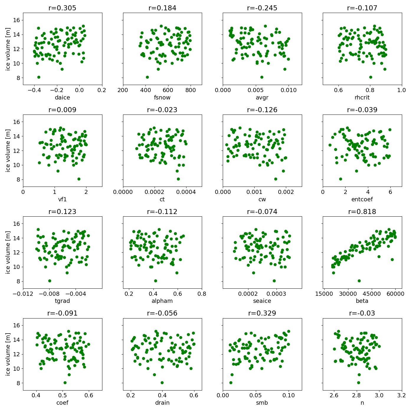
Figure 9 Relation between ice volume of Greenland at 5000 ice years in FAMOUS-BISICLES and each parameter. Ensemble members satisfying the GMST constraint are used. Correlation values are displayed on the top of each panel.

3.3 Responses of the Greenland ice sheet

The Greenland ice sheet also shows various responses to modifications in the parameters in the ensemble of simulations, ranging from 8 to 15 m SLE (Fig. 9). The simulated range is similar to the range in the reconstructions, suggesting 9.3 to 12.3 m SLE (7.3 m + 2 ∼ 5 m SLE, Clark and Mix, 2002; Lecavalier et al., 2014; Bradley et al., 2018; Tabone et al., 2018), while the model overestimates the higher band.

Interestingly, the results show a different sensitivity to the model parameters we vary compared to the North American ice sheet (Fig. 9). The variations in the ice volume are mostly explained by changes in beta, where higher values increase the friction between the ice sheet and the bedrock at a cold ice base. This acts to increase the ice volume by reducing the amount of ice transported to its margin, which then calves at the continental shelf, and hence by inducing thickening of the ice sheet interior.

The lower sensitivity of the Greenland ice sheet to albedo parameters comes from different climatic conditions compared to North America. In North America, the large area is covered by negative surface mass balance (Fig. 3g) as the summer temperature can be close to freezing point in the simulations (Fig. 10). Hence, albedo parameters cause a drastic difference since they control the magnitude of the negative SMB over North America (Fig. 8). In contrast, the Greenland ice sheet is covered by colder conditions in summer (Fig. 10); hence, most surface areas have positive surface mass balance (Fig. 9). Under this condition, the amount of the ice loss is determined by the amount of ice transported from the interior to its edge, which then calves. As a result, the ice volume is mainly driven by beta since it controls the transport of ice under the cold ice base.

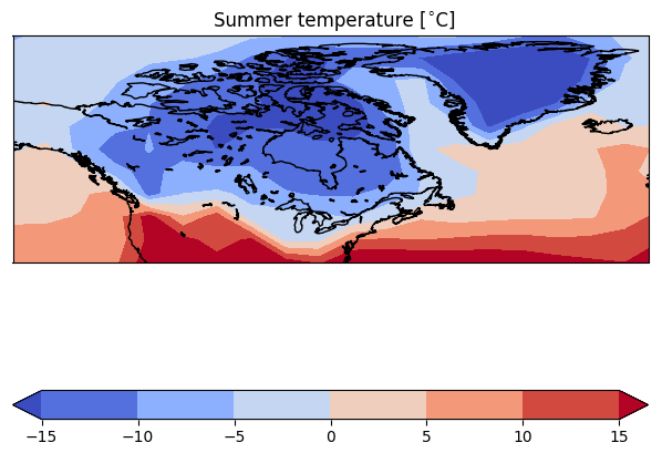
Figure 10 Summer surface air temperature (°C) over North America and Greenland, averaged over all ensemble members satisfying the GMST constraint.

Previous studies have shown that basal melting of ice shelves by the underlying ocean is also important in controlling Greenland ice sheet volume at the LGM in their coupled ice shelf–ice sheet models (Bradley et al., 2018; Tabone et al., 2018). In this study, however, a constant value was given for the ice shelf basal melting. Conducting ensemble simulations with variations in the amount of ice shelf melting may enable us to explore their relative importance.

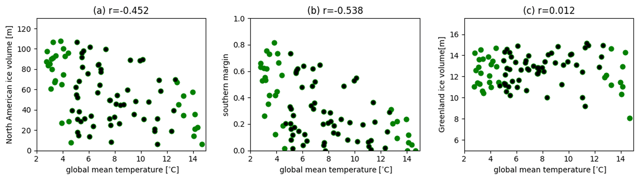
Figure 11 Relationship between GMST (°C) and ice sheet variables. (a) North American ice sheet volume (m), (b) ratio of southern extent of the North American ice sheet compared to Dalton et al. (2020) and (c) Greenland ice sheet volume (m). Ensemble members that satisfy the GMST constraint and have run 5000 ice sheet years are used (87 members). Correlation values are also shown in each figure. Black dots show results within the 2σ uncertainty in the LGM GMST (8.7 °C ± 4.0 °C).

3.4 Effects of global mean surface temperature (GMST) on ice sheet volume

The sensitivity of the ice sheets to the reasonable LGM GMST range (2.7–14.7 °C) is explored to see the relationship between them (Fig. 11). The results show a high correlation between the GMST and North American ice volume and southern extent; colder climates correspond to larger and more extensive ice sheets (Fig. 11a and b). This is not a surprise since a large uncertainty of ± 6.0 °C is applied to the GMST. Reducing the uncertainty level to 2σ (8.7 °C ± 4.0 °C, black dots in Fig. 11) weakens the correlation between the GMST and the North American ice volume and southern extent to −0.193 and −0.285, respectively. Nevertheless, the correlation analysis still shows some sensitivity of the southern extent of the North American ice sheet to GMST (Fig. 11b), where a colder global climate tends to produce a more extensive ice sheet in the south. In other words, it can also be said that it is hard to get an extensive southern North American ice sheet under warm LGM GMST (above 12.0 °C), irrespective of the albedo parameters, which demonstrates the value of constraining the upper band of real LGM temperatures for simulating the North American ice sheet well.

The Greenland ice sheet appears to be insensitive to the reasonable LGM GMST range (2.7–14.7 °C), which is consistent with the dominant role of basal sliding in controlling the ice volume. Reducing the uncertainty level to 2σ (8.7 °C ± 4.0 °C, black dots in Fig. 11) increases the correlation value to 0.259, possibly associated with an increase in snowfall following the warming climate; however, the effect is much weaker compared to the effect of basal sliding.

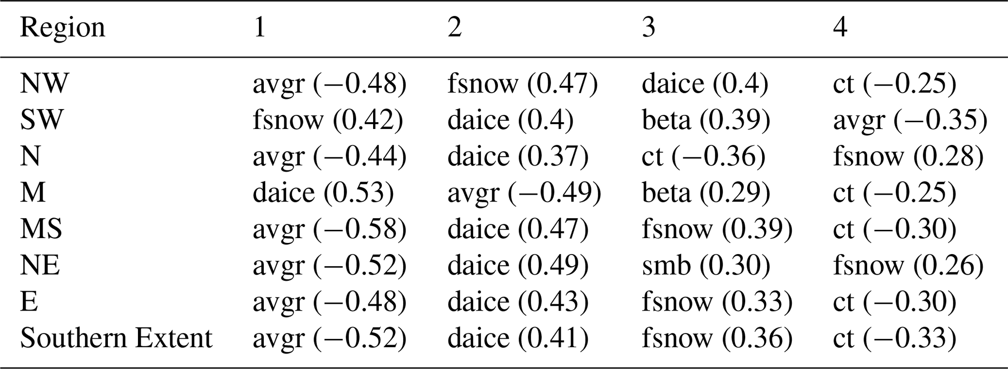
Table 2 Four most influential parameters on ice volumes at different regions. Values in the bracket show the correlation. For the Southern Extent, results from Fig. S4 are used.

3.5 Localities in the effect of parameters

The different sensitivities to parameters between the North American and Greenland ice sheets imply that similar variations in sensitivity to parameters may exist between different local regions within the huge North American ice sheet. To explore this point, we separate the North American ice sheet into seven different sectors (NW, SW, N, M, MS, NE, E) where a substantial amount of ice remains in the ensemble mean of members satisfying the GMST constraint (Fig. 12). Results are summarised in Table 2. While the albedo parameters remain the most important ones (daice and avgr) in each region, we find that beta has an increased influence in SW and M. These areas either exhibit a mountainous bedrock topography or have very thick ice, and hence they can be more affected by the basal sliding parameters. Additionally, we find that ct has a relatively strong influence on the northern (N) and eastern (E) parts of the North American ice sheet. Our analysis indicates some variation in regional sensitivities to climate and ice sheet parameters in different sectors of the ice sheet sectors. Further analysis beyond the scope of this study would be required to explore this regional dependency in detail.

Figure 12 Six different areas (NW, SW, N, M, NE and E) of the North American ice sheet used for the additional analysis (black rectangle). Blue shades show the mean ice thickness (m, colour) of members satisfying the GMST constraint.

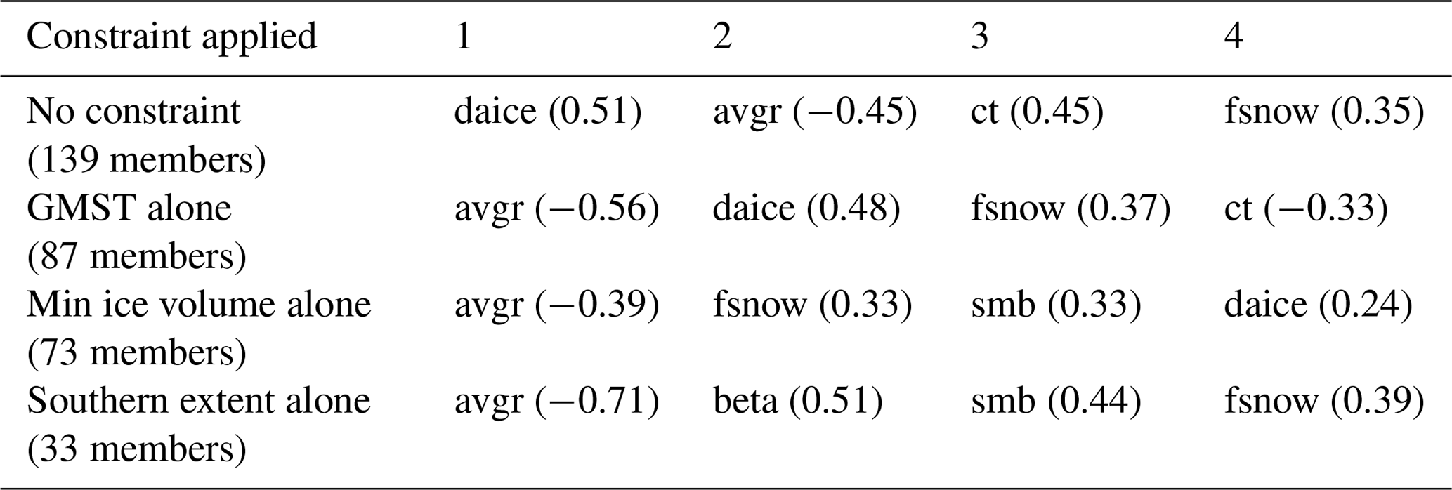
Table 3 Effects of constraints on the relation between parameters and North American ice sheet volume at year 5000. The four most influential parameters on ice volumes are shown.

3.6 Sensitivity of influential parameters to individual constraints

Applying our three simulation constraints simultaneously may be hiding relationships that exist between model parameters and simulation behaviour. We perform additional analyses to explore how each constraint individually affects the relationship between our model parameters and North American ice sheet volume. In the case of no constraints (139 members), the albedo parameters are important, but the influence from ct becomes more important (Table 3). This is due to the increased range of GMST allowed by varying ct (Fig. 5). Having a much colder or warmer climate allows the ice sheets to grow or melt, and the resulting feedback further enhances the role of ct. In contrast, most members with extremely warm climates crashed during the 5000-year simulation. This means that entcoef does not appear to have so large an effect on ice sheet volume directly, unlike its importance in setting the GMST.

In the case of applying only the ice sheet volume constraint (73 members), avgr and fsnow still show relatively high correlations with ice sheet volume. However, their influence is less than when GMST constraint alone is applied (Table 3). The ice volume constraint alone results in a preferred selection of members exhibiting colder climates (46 members have a GMST below 4 °C). As a result, the members are less sensitive to albedo related parameters.

When the southern extent constraint alone is applied, 33 members remain. Similar to above, members satisfying this condition tend to have very cold climates, where 24 members have GMST colder than 4 °C and 14 members colder than 0.63 °C. In this case, avgr and beta appear to be most influential. This may imply that snow albedo and basal conditions play an important role in maintaining an extensive ice sheet once the climate allows the ice sheet to reach this size. Further discussion on the maintenance of the southern margin of the North American ice sheet is in Sect. 4.1.

4 Discussion

4.1 How could FAMOUS-BISICLES be made to reproduce the southern extent of the North American ice sheet?

A recent study by Gandy et al. (2023) performed a similar ensemble simulation with FAMOUS-Ice but with fixed SSTs and with the simpler Glimmer ice sheet model rather than BISICLES. Our findings here are consistent with theirs in that the ice extent is sensitive to choices of parameters in the snow and ice albedo scheme and that both models underestimate the southern extent of the North American ice sheet, especially the so-called “lobe” characteristics. To investigate the possibility of the model being able to reproduce the full extent of the southern margin of the North American ice sheet, we analyse in detail the ensemble member that has the most extensive southern margin, disregarding our imposed climate plausibility constraints (Fig. 3e). In this simulation, the performance of the southern extent of the North American ice sheet is closer to the reconstructed area due to the very cold climate simulated, whose absolute GMST is −7.4 °C. Yet even in this very cold simulation, the model cannot maintain the “lobe” characteristics of the North American ice extent as far south as the reconstructions.

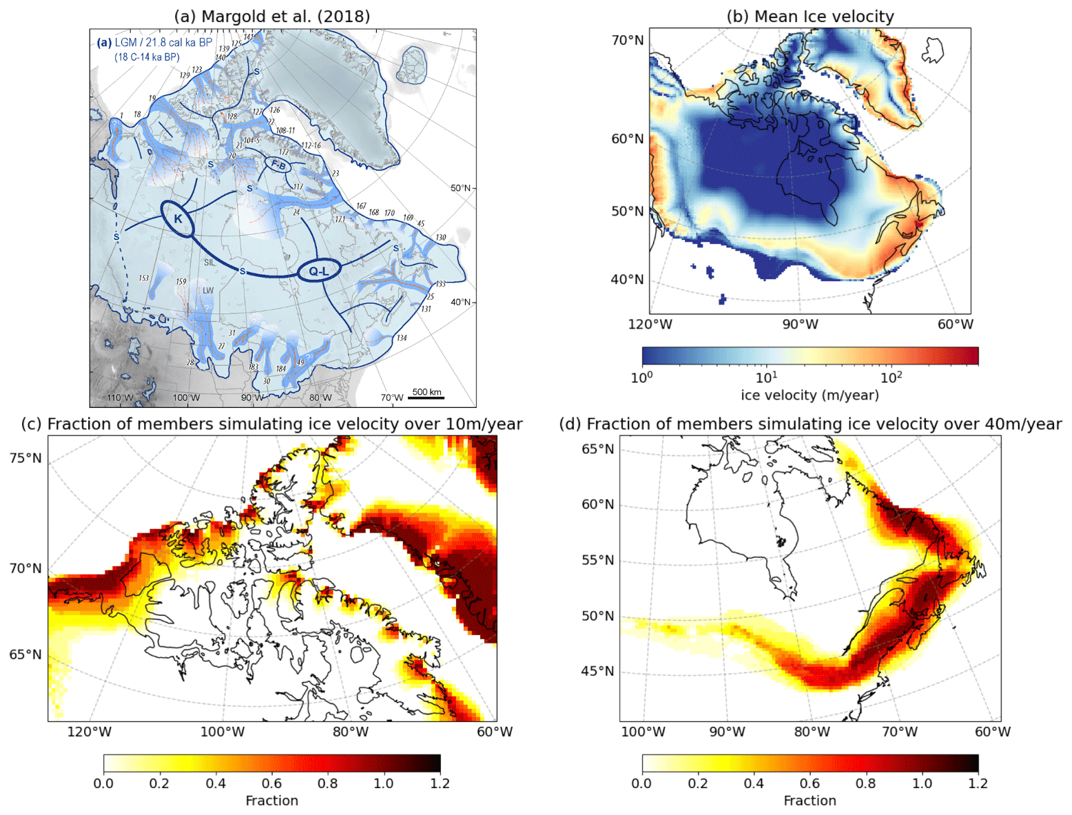
Figure 13 Comparison of ice velocity (m yr⁻¹, colour) between (a) reconstruction (Margold et al., 2018, adapted from Fig. 5 of Margold et al., 2018) and (b) the mean of the best 16 members. Panels (c) and (d) show the fraction of numbers of members simulating ice velocity beyond 10 m yr⁻¹ and 40 m yr⁻¹, respectively. Fraction of 1.0 means all of the 16 members simulate ice velocities of those values.

So, how might we reproduce the southern margin of the North American ice sheet in our simulations? There are several possibilities.

• Finer horizontal resolution in the climate model. During the simulations, FAMOUS-BISICLES loses the thin ice sheet at the south margin abruptly in the first 1000 ice sheet years due to the very large negative SMB simulated in the atmospheric model (e.g. Fig. 13b). Applying a high-resolution atmospheric model might be better able to sustain a more southerly ice margin through a stronger stationary wave effect that cools the area (Abe-Ouchi et al., 2007).

• Representation of clouds. Gregory et al. (2012) pointed out the importance of changes in cloud cover over the southern margin of the North American ice sheet on its SMB during the glacial inception. Having a larger cloud cover at the southern margin may help to maintain the ice sheet by reducing the very large negative SMB, although a careful analysis on the physical plausibility of creating this feature would need to be done.

• Improvements in the downscaling scheme. Including the effect of strongly stratified boundary layer on the surface temperature during the downscaling may allow a colder surface temperature over ice, which can help sustain the ice sheet at its margin. Incorporation of downscaling of accumulation in FAMOUS-BISICLES can increase the snowfall at the southern margin, which increases the SMB and surface albedo and may help to sustain the ice sheet at the southern margin (e.g. Yamagishi et al., 2005).

• Higher initial surface elevation. The simulation could be started with a higher initial surface elevation, which can be obtained by giving a thicker ice or a higher bedrock topography at the southern margin, allowing for lower surface temperatures due to the higher elevation, although this may not be physically plausible.

• Paleo-vegetation. The choice of vegetation type for the unglaciated region near to the ice sheet may be relevant. The modern vegetation distribution used in this study may tend to give a warmer condition in this area, unlike tundra, which grows under cold climates and causes a surface cooling (O'ishi and Abe-Ouchi, 2013).

• Bedrock conditions. Creating a slippery bedrock condition would enhance ice flow from the ice sheet interior towards the margin, and thus they may be instrumental in redistributing ice outwards. In this regard, adding a scheme that allows the generation of proglacial lakes and increases ice flow at the southern margin would help advance the lobe (Hinck et al., 2022).

• Longer integration of the model. Extending the integration of FAMOUS-BISICLES may help to redistribute the thick ice in the interior to the southern margin. In fact, some of the members that have been extended for additional 5000 years show some southward expansion (Fig. S2).

It is also possible that the concept of the southern margin being in a quasi-equilibrium state with the LGM forcing may not be valid, and it may instead be the case that several transient ice advance events occurred during the recent glacial period (and preceding the LGM) (e.g. Pico et al., 2017; Gowan et al., 2021; Bradley et al., 2024). We speculate that such earlier southward ice advance may allow a more expansive southern ice sheet to establish before rebalancing with the insolation forcing. In this case, running a long transient simulation, rather than performing equilibrium-type LGM simulations, may be essential for achieving the target southern margin extent.

4.2 Performances of ice streams

The positions of our simulated ice streams in the best 16 ensemble members are evaluated against the reconstruction by Margold et al. (2018) (Figs. 13 and S5). The figure shows that BISICLES shows regions of relatively high ice velocities (or ice streams) at various sites, despite the relatively low resolution of the model (16 km at finest grid) and the relatively short integration period. Specifically, most members reproduce high ice velocities at the margin over the Baffin Bay area. In addition, the simulation of ice streams facing the Arctic Ocean is encouraging (Figs. 13 and S5). However, once again the southern margin is tricky to get right, and our ice stream behaviour there is somewhat diffuse, not picking up the characteristic “lobe” structure of the reconstructions (Margold et al., 2018). Over the eastern North American ice sheet, the model captures some large glaciers, such as the Laurentian Channel (25), Placentia Bay–Halibut Channel (133) and Hopedale Saddle (168), while none of the best 16 ensemble members simulate the large ice stream that flows to the Labrador Sea from the present-day Hudson Bay area. These poorly represented ice stream features may be caused by the low resolution of the smallest ice sheet refinement (16 km, e.g. Gandy et al., 2019), too-short integration and misrepresentation of the surface type of till (Gowan et al., 2019). With the last point, the amount of till water calculated prognostically in the simulations appears small; hence, most areas use the Weertman sliding law. An increase in the basal melting, a choice of a smaller value for drain or incorporating a spatially variable Weertman coefficient map based on geological evidence may help to improve the performance of the ice streams. Nevertheless, the model does show some reasonable potential in simulating North American ice streams considering the relatively low resolution and the explicit calculation of basal drag.

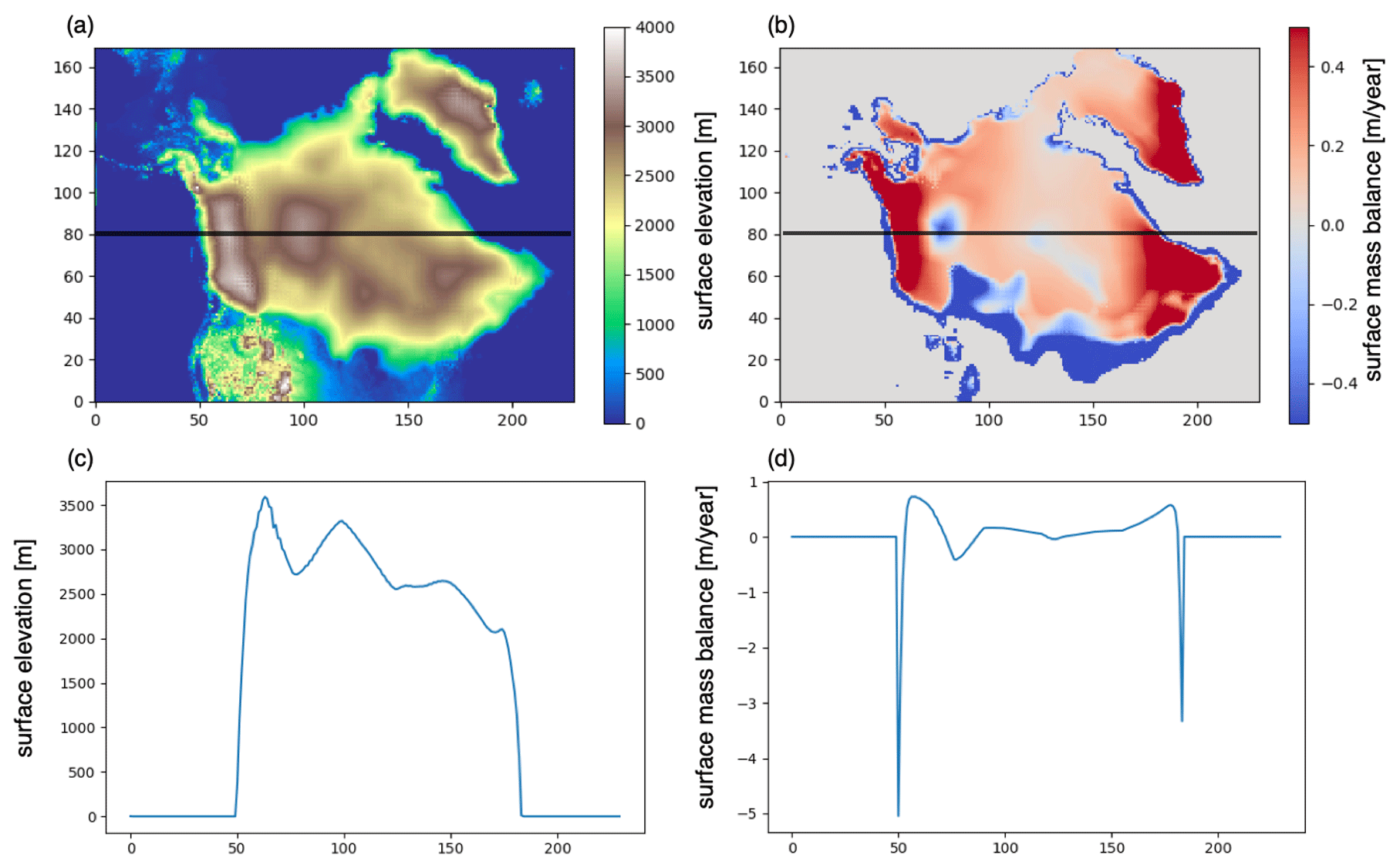
Figure 14 An example of local ice melting in the interior of the ice sheet using ensemble member xplji, which has a GMST of 9.9 °C and North American ice sheet volume of 88.4 m SLE. (a) Surface topography (m), (b) surface mass balance (m yr⁻¹), and height zonal cross-section of (c) surface topography and (d) surface mass balance at y = 80 are shown.

4.3 Effects of biases in the simulated climate

Some of the simulations in the ensemble exhibit a local melting of the ice sheet from parts of the interior outwards, which is unusual as ice sheets usually melt from their margins, where the surface temperature is close to the freezing point (e.g. Figs. 3c and 14). This phenomenon is caused by biases in the atmospheric model, which are amplified by the downscaling method and a positive feedback from the coupling. In these simulations, the model has a warm summer temperature bias over the ice sheet interior. As a result, large parts of the central North American ice sheet have a temperature above −10 °C despite the surface elevation exceeding 2000 m (Fig. 10). A similar feature was pointed out by Smith et al. (2021a) using the same model under the modern Greenland ice sheet, which produced a higher ELA (around 2 km in height in places) compared to a high-resolution regional atmospheric model (at about 1 km in height). Second, because the downscaling of SMB strongly depends on the elevation, a local change in surface elevation can induce a local negative surface mass balance if the surface temperature calculated in the FAMOUS grid points are close to the freezing point. This example is shown in Fig. 14, where a negative SMB can be found at the local minima of surface elevation, despite the elevation exceeding 2000 m. The initial negative SMB then kicks in a strong positive feedback where melting of snow reduces the albedo and results in more energy absorption. As a result, the ice elevation starts to decrease and causes additional positive feedback similar to saddle node collapse (Gregoire et al., 2012). The strong dependence of SMB on temperature and altitude implied by this way of downscaling the climate model output works well for modern Greenland, especially at low elevation where the SMB is observed to have a very strong elevation dependence. However, at the higher altitudes achieved by the LGM North American ice sheet, SMB may be more greatly affected by other factors such as wind speeds, as suggested by studies on Antarctica (Van Liefferinge et al., 2021). Hence, further improvements in the downscaling method at higher elevation could help to reduce the impact of the climate biases.

5 Conclusion

In this paper, we have presented a large ensemble of simulations of the North American and Greenland ice sheets and climate of the LGM, performed with a coupled atmosphere–ice sheet–slab ocean model FAMOUS-BISICLES, a version of the FAMOUS-Ice model developed by Smith et al. (2021a). The experiment consists of a 200-member perturbed parameter ensemble, where the values of 16 parameters associated with climate and ice dynamics were varied using a Latin hypercube sampling method. The simulated results are evaluated against the LGM GMST, the North American ice volume and the southern extent of the North American ice sheet. In the ensemble, the GMST is controlled by a combination of precipitation efficiency in the large-scale condensation and entrainment rate in the cumulus convection, consistent with previous FAMOUS simulations of modern climate (Joshi et al., 2010). Under reasonable LGM GMST conditions, we find that the surface albedo exerts the strongest control on North American ice volume. In contrast, the ice volume of Greenland is found to be mainly controlled by the Weertman coefficient in the basal sliding law. The different sensitivity of these ice sheets to the model's physical parameter values mainly comes from different climatic conditions. The North American ice sheet, being generally warmer, has a larger area of negative SMB, which is affected by the albedo. In contrast, most parts of the Greenland ice sheet are covered by a very cold atmosphere, meaning that the ice sheet volume is more affected by the calving at its margin, the total amount of which is controlled by the magnitude of the basal sliding law that affects the amount of ice transported to the margins. These differences between the North American and Greenland ice sheets provide an important take-home message on model performance, suggesting that for the best flexibility (i.e. the ability to simulate conditions very different from today), simulators should be calibrated under a range of climate and ice sheet conditions and tested in an out-of-sample manner.

Analysis of the relationship between the North American southern ice extent and GMST with the uncertainty level of 2σ (8.7 °C ± 4.0 °C) shows a slightly weak relation. Nevertheless, we find that it is hard to get an extensive southern North American ice sheet under warm LGM global temperature (above 12.0 °C), irrespective of the albedo parameters in our model. This demonstrates the value of constraining the upper band of real LGM temperatures for simulating the North American ice sheet well.

Based on our plausibility constraints, the model produces 16 “acceptable” simulations with reasonable GMST and North American ice sheet values. These simulations show the most extensive southern margin under reasonable LGM temperature and ice volume, but, like LGM ice sheet simulations by other authors, they overestimate ice volume in Alaska and do not expand far enough at the southern margin (even after 5000 years, with the absolute global temperature as cold as −7.4 °C). Both of these features are likely attributable to the underestimation of the stationary wave effect (Roe and Lindzen, 2001; Abe-Ouchi et al., 2007), which might be improved upon or overcome by increasing the climate model resolution. It is also possible that more accurate representation of the palaeo vegetation, different treatments of ice sheet sliding and downscaling method of the SMB, or a different spin-up procedure could improve the simulated southward ice sheet extension.

Our results show that warm summer temperature biases in the interior of the ice sheet and the downscaling method of SMB based on elevation can cause strong local melting of the ice sheet from the interior outwards. More complex treatment of the atmospheric conditions and surface mass balance in the ice sheet interior could improve this, and may be especially important when applying the model to the Antarctic ice sheet.

Lastly, the strong sensitivities of the North American ice sheet to albedo at the LGM may imply a potential constraint on the future Greenland ice sheet by constraining the formulation and behaviour of albedo schemes for climate and ice sheet models under relatively warm climates. Running similar ensemble simulations with a directly comparable version of this model for the modern and future Greenland ice sheet will provide an important data set to directly connect the simulations of past climates and ice sheets to those of modern and future conditions. Using such data, we will be able to explore how simulations of past climate–ice sheet conditions can more tightly constrain or increase confidence in projections of future sea level rise.