Continuous synchronization of the Greenland ice-core and U–Th timescales using probabilistic inversion

This study presents the first continuously measured transfer functions that quantify the age difference between the Greenland ice-core chronology 2005 (GICC05) and the U–Th timescale during the last glacial period. The transfer functions were estimated using an automated algorithm for Bayesian inversion that allows inferring a continuous and objective synchronization between Greenland ice-core and East Asian summer monsoon speleothem data, and a total of three transfer functions were inferred using independent ice-core records. The algorithm is based on an alignment model that considers prior knowledge of the GICC05 counting error but also samples synchronization scenarios that exceed the differential dating uncertainty of the annual-layer count in ice cores, which are currently hard to detect using conventional alignment techniques. The transfer functions are on average 48 % more precise than previous estimates and significantly reduce the absolute dating uncertainty of the GICC05 back to 48 kyr ago. The results reveal that GICCC05 is, on average, systematically younger than the U–Th timescale by 0.86 %. However, they also highlight that the annual-layer counting error is not strictly correlated over extended periods of time and that within the coldest Greenland Stadials the differential dating uncertainty is likely underestimated by up to ∼13 %. Importantly, the analysis implies for the first time that during the Last Glacial Maximum GICC05 may overcount ice layers by ∼10 % – a bias possibly attributable to a higher frequency of sub-annual layers due to changes in the seasonal cycle of precipitation and mode of dust deposition to the Greenland Ice Sheet. The new timescale transfer functions provide important constraints on the uncertainty surrounding the stratigraphic dating of the Greenland age scale and enable an improved chronological integration of ice cores as well as U–Th-dated and radiocarbon-dated paleoclimate records on a common timeline. The transfer functions are available as a Supplement to this study.

1 Introduction

The Greenland ice-core chronology 2005 (GICC05; Rasmussen et al., 2006; Svensson et al., 2008) and the U–Th timescale (e.g., Cheng et al., 2016) are among the most widely used independently dated chronological frameworks of the last glacial period. The timescales not only provide the backbone of some of the most unique and detailed records of global climate change, but their robustness makes them exceptionally suited for resolving the temporal structure of Dansgaard–Oeschger (DO) events and other abrupt climate shifts.

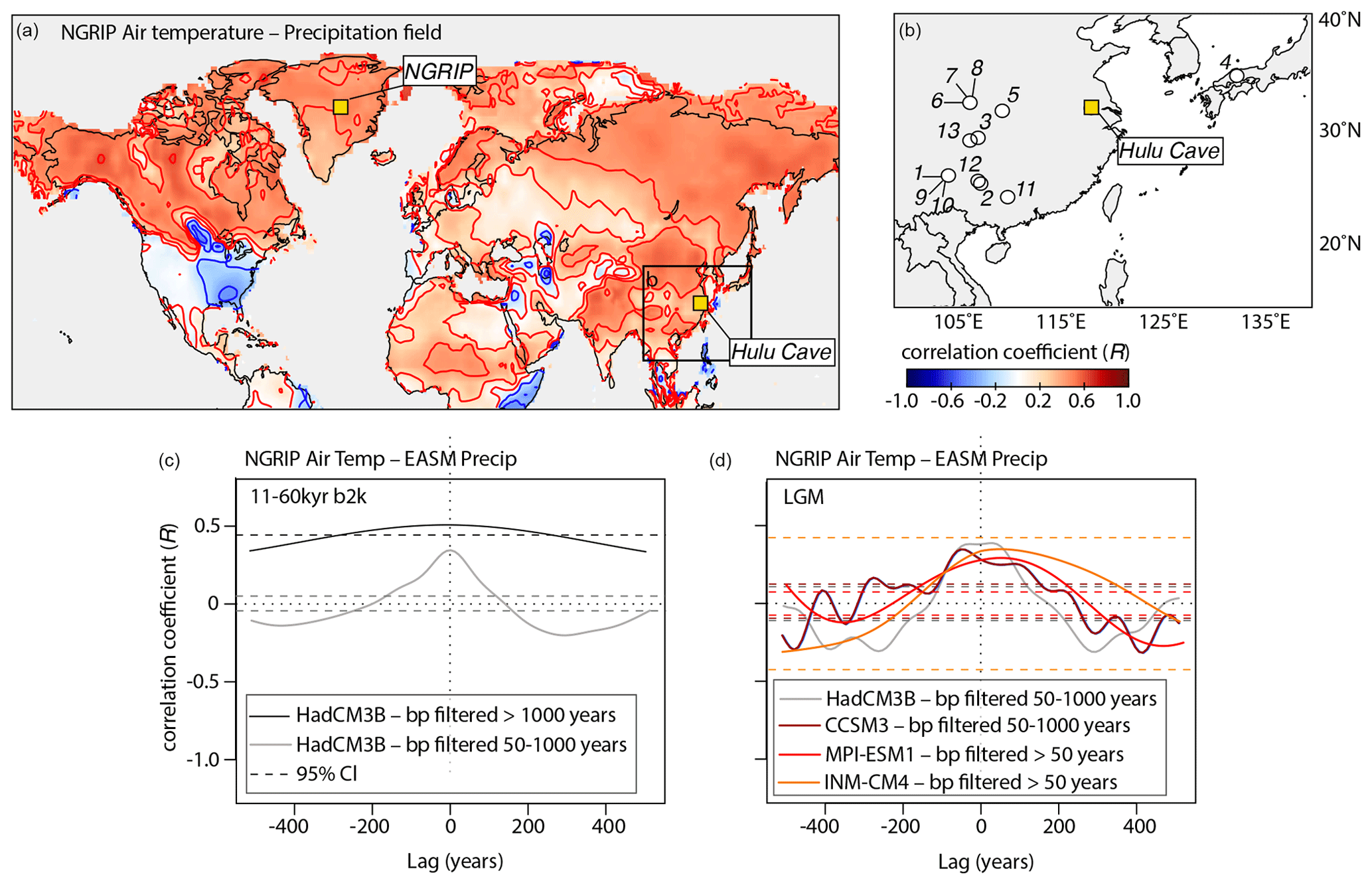
Figure 1 (a) Instantaneous (lag 0) spatial correlation between mean decadal surface air temperature at the NGRIP site and mean decadal land surface temperatures during the last glacial period (11–60 kyr b2k) as simulated with the HadCM3B-M2.1 coupled general circulation model (Armstrong et al., 2019). The simulation incorporates Dansgaard–Oeschger cycles, Heinrich events, and shorter-term variability, with a spatial climate fingerprint derived from a Last Glacial Maximum (LGM) freshwater hosing experiment applied over the North Atlantic Ocean. The locations of NGRIP, the East Asian summer monsoon (EASM) region, and Hulu Cave are also shown. (b) EASM domain showing the location of speleothem records compiled by Corrick et al. (2020) and used in this study. 1. Dashibao; 2. Dongge; 3. Furong; 4. Maboroshi; 5. Sanbao; 6. Shizi; 7. Songjia1; 8. Songjia3; 9. Wulu3; 10. Wulu32; 11. Xiaobailong; 12. Yamen; 13. Yangkou. Reference to the cave site is provided in Corrick et al. (2020). (c) Cross-correlation between simulated NGRIP air temperature and EASM precipitation between 11 and 60 kyr ago. The EASM region is defined here as the average of 10–40° N and 95–125° E. The time series were bandpass-filtered to quantify leads and lags at millennial and shorter timescales, respectively. (d) Same as (c) but for the LGM using transient climate model simulations (Armstrong et al., 2019; Liu et al., 2009) and equilibrium experiments from CMIP6 (Kageyama et al., 2021). Results from HadCM3B and CCSM3 span the interval ∼17.5–21 kyr b2k, whereas for CMIP6 only simulations longer than 200 years were considered for the cross-correlation analysis. Dashed lines reflect the 95 % significance level against first-order autoregressive (AR1) noise.

The GICC05 is based on annual-layer counting back to 60 kyr before 2000 CE (b2k) and due to the incremental nature of the counting uncertainty, it provides high internal consistency that enables accurate relative age estimates of climate events. The Greenland ice-core timescale underpins a number of high-resolution ice-core records of North Atlantic climate and atmospheric composition. These records have become established Northern Hemisphere templates for the last glacial period and have shaped our understanding of the physical mechanisms driving rapid climate shifts (Andersen et al., 2004; Dahl-Jensen et al., 1998; Legrand and Mayewski, 1997; Schüpbach et al., 2018) and their rates of change (Jansen et al., 2020). By contrast, the U–Th timescale is constructed using high-precision U–Th dating, which yields much smaller uncertainty in the absolute ages than GICC05 during the last glacial. The U–Th timescale provides a temporal framework for speleothem δ¹⁸O data, which are largely dominated by records falling into the East Asian summer monsoon (EASM) domain (Corrick et al., 2020) (Fig. 1); altogether, records from this region constitute a key blueprint of low-latitude hydroclimate variability, integrating intensity changes in East Asian monsoon and meridional shifts of the Intertropical Convergence Zone (ITCZ; Wang et al., 2001, 2006).

Both the GICC05 and U–Th timescales serve to test, improve, and constrain chronologies for a wide range of paleoclimate archives and proxy records. These age scales have been used to validate and benchmark Antarctic ice-core chronologies (e.g., Buizert et al., 2015; Sigl et al., 2016), which ultimately enable resolving the interhemispheric phasing of DO events (Buizert et al., 2018) and the rate of greenhouse gas emissions during the last glacial period (Bauska et al., 2021). They are also widely used to constrain paleoceanographic records with poor independent age control (Bard et al., 2013; Hughen and Heaton, 2020; Waelbroeck et al., 2019). To build a chronology for deep-sea sediment cores, proxy signals are commonly correlated with abrupt cooling and warming events observed in ice-core proxies or speleothem δ¹⁸O under the assumption of direct synchrony of climate changes. These climatically tuned chronologies, despite limiting our ability to test leads and lags between oceanic and atmospheric processes (Henry et al., 2016; Hughen and Heaton, 2020), still lay the foundations for deriving “best-guess” temporal constraints on a variety of fundamental boundary conditions of glacial ocean circulation and its coupling with the atmosphere system.

Because the Greenland ice-core and U–Th chronologies are constructed independently, the occurrence of systematic timescale offsets and dating biases of the order of hundreds of years complicates the comparisons of events integrated in the proxy records that hinge on these timescales. Perhaps more importantly, the chronology that forms the older portion of the new IntCal20 radiocarbon calibration curve is dominantly reliant on the Hulu Cave speleothem U–Th timescale (Cheng et al., 2016, 2018; Reimer et al., 2020; Southon et al., 2012). During the period spanning ∼14–54 kyr b2k, a wealth of ¹⁴C datasets have been placed on the Hulu Cave U–Th timescale either indirectly via stratigraphic tuning of paleoclimate data to the high-resolution Hulu δ¹⁸O record (Bard et al., 2013; Darfeuil et al., 2016; Hughen and Heaton, 2020) or more directly by means of ¹⁴C wiggle matching (e.g., Bronk Ramsey et al., 2020; Turney et al., 2010, 2016). As a result, potential differences between the timescales – if not quantified and corrected for – can hinder a proper assessment of ¹⁴C-dated environmental and archeological records within the ice-core climatic framework.

Furthermore, knowledge of the existing timescale offsets is important for high-resolution studies of marine ¹⁴C (e.g., Muschitiello et al., 2019). This is crucial for reconstructions whose chronologies are more conveniently anchored to ice-core records rather than the Hulu Cave speleothems, as is often the case for North Atlantic sediment cores that integrate common regional climatic changes (Skinner et al., 2019; Thornalley et al., 2015; Waelbroeck et al., 2019) or sites where isochronous tephra deposits can be traced between ice cores and marine records (e.g., Ezat et al., 2017; Sadatzki et al., 2019). In these instances, potential discrepancies between the GICC05 and U–Th timescales can lead to an imprecise assessment of ocean Δ¹⁴C relative to those of the atmosphere inferred from the IntCal datasets, thus affecting the estimation of ocean radiocarbon inventories.

In turn, resolving the differences between the GICC05 and U–Th timescales can help to reduce and characterize their absolute dating uncertainty and facilitate the comparison of ice cores and radiocarbon-dated records on a common timeline. Altogether, this is pivotal to advancing our understanding of the physical mechanisms behind abrupt climate change and to harmonizing climate, environmental, and archeological records of the last glacial cycle.

There are two main types of synchronization to integrate the GICC05 and U–Th timescales: (i) synchronization of climate records and (ii) synchronization of cosmogenic radionuclide data. The first is based on correlation of climatic signals integrated in Greenland ice-core records and speleothem δ¹⁸O that are assumed to be synchronous. The second is based on the correlation of externally forced and essentially climate-independent variations in ice-core ¹⁰Be and Hulu Cave ¹⁴C records.

Despite the circularity that climate synchronization entails, such as precluding testing the synchronicity of teleconnections between Greenland and the East Asian monsoon system, the concerns about a potentially large climate phasing between polar ice-core and EASM speleothem records during the last glacial period have been put to rest. Unlike other regions where there are potentially complex site-specific responses to large-scale change (Adolphi et al., 2018), currently there is ample evidence that the North Atlantic and Asian monsoon climates are coupled on short atmospheric timescales (e.g., Adolphi et al., 2018; Corrick et al., 2020; Cvijanovic et al., 2013) – i.e., likely shorter than the mean resolution of the proxy records used for climate synchronization. The teleconnection mechanism, which is likely modulated by variations in the Atlantic Meridional Overturning Circulation, is well documented and involves coherent meridional shifts of the midlatitude storm tracks, the ITCZ, and the related monsoon systems (e.g., Ceppi et al., 2013; Kageyama et al., 2013; Zhang and Delworth, 2005). This is further supported by climate model simulations, which demonstrate that this atmospheric coupling synchronizes the North Atlantic and EASM region down to multidecadal timescales – a teleconnection that is robust under different glacial boundary conditions (Fig. 1c and d).

Since the construction of the GICC05 chronology, climate synchronizations between Greenland and EASM speleothem records (e.g., Hulu Cave) have been derived by identification of tie points marking sharp transitions in both the ice-core and speleothem stratigraphies (e.g., DO events). The synchronization approach has been performed either by manual, qualitative comparison of the climate records (Corrick et al., 2020; Svensson et al., 2006, 2008; Weninger and Jöris, 2008) or using reproducible, quantitative methods for detecting change points (Adolphi et al., 2018; Buizert et al., 2015). While tie points associated with sharp climate transitions are suitable for proxy synchronization as they typically have a high signal-to-noise ratio, at present, the main methodological drawback of this approach is that it relies on only a discrete set of stratigraphic markers, which prevents quantifying the alignment uncertainties in a continuous fashion.

The approach for synchronizing cosmogenic radionuclide records involve sliding window techniques, such as cross-lagged regression (Muscheler et al., 2014) or more commonly Bayesian wiggle matching (BWM; Adolphi and Muscheler, 2016). The techniques aim at matching relative changes in ¹⁰Be and ¹⁴C concentrations over a series of time windows and focusing on centennial to multi-centennial variations that are typically dominated by solar-induced – and largely periodic – changes in production rates (Vonmoos et al., 2006). Synchronization using BWM offers high precision and has proved effective during the Holocene when the offsets between the ice-core and ¹⁴C timescales are mostly systematic (Adolphi and Muscheler, 2016; Sigl et al., 2016). However, these matching techniques depend heavily on the predefined window length (e.g., Schoenherr et al., 2019) and can lead to biased conclusions about synchrony if the timescale offsets change faster than the time window used for matching. Specifically, BWM only produces a single point of match for each window analysis, which generally spans 1000 to 5000 years, thus averaging out any short-term, nuanced fluctuations in the timescale difference (Adolphi et al., 2018; Adolphi and Muscheler, 2016). As the method leans on analyzing overlapping windows, on one hand it can lead to neighboring offset estimates of the BWM being positively correlated, which results in smoothing out the timescale transfer function. On the other hand, it may lead BWM to identify wrong correlation, thus yielding sudden – and potentially spurious – jumps in the timescale offsets (Muscheler et al., 2014; Muschitiello et al., 2019).

With climate synchronizations standing on a limited number of stratigraphic tie points and the latest alignment of cosmogenic radionuclides on only five BWM estimates (Muscheler et al., 2020), a new continuous synchronization between the GICC05 and U–Th timescales for the last glacial period is urgently required. In particular, the recent revision of the high-resolution Hulu Cave δ¹⁸O record (H. Cheng et al., 2016, 2021) with an updated U–Th chronology (H. Cheng et al., 2018, 2021) provides further motivation for re-assessing the synchronization between the Greenland ice-core and U–Th timescales. Lastly, there is a need for improved constraints during the Last Glacial Maximum (LGM), i.e., when the timescales reach their largest offset according to cosmogenic radionuclides (Adolphi et al., 2018; Sinnl et al., 2023), and assess possible fast changes in the timescale difference that are currently challenging to detect.

In this study, some of these limitations are addressed by applying an automated probabilistic synchronization method to produce the first continuous transfer functions that quantify the offset between the GICC05 and U–Th timescales. The method minimizes the misfit between ice-core and speleothem proxy records while accounting for prior knowledge of the uncertainty in annual-layer identification in ice cores using a Bayesian inversion of the GICC05 maximum counting error (MCE) (Rasmussen et al., 2006; Svensson et al., 2008). To minimize noise due to site-specific environmental factors and U–Th dating uncertainties, the speleothem records are integrated using a Monte Carlo principal component analysis procedure that isolates the common EASM hydroclimatic pattern and estimates uncertainties. The new timescale transfer functions considerably improve the precision of earlier estimates and reduce the absolute dating uncertainty of GICC05 in the interval ∼11–48 kyr b2k. The results also indicate large and fast fluctuations in the timescale difference during the LGM and other cold stadial periods, suggesting previously unrecognized biases in the ice-core annual-layer counting. The implications of these findings are discussed.

2 Data and methods

2.1 Proxy data and Monte Carlo principal component analysis

The offsets between the GICC05 and U–Th timescales were estimated by performing three synchronizations based on independent Greenland ice-core climate proxy records (CLIM). The proxy data used in this study are presented in Fig. 2. The CLIM synchronizations were established over the period ∼11–48 kyr b2k using high-resolution Ca²⁺ concentrations of mineral dust from NGRIP (CLIM1) (Erhardt et al., 2019), δ¹⁸O data from NGRIP (CLIM2) (Andersen et al., 2004) and GRIP (CLIM3) (Johnsen et al., 1997), respectively (all on the GICC05 timescale), and revised δ¹⁸O data from EASM speleothems on their independent U–Th chronologies (Corrick et al., 2020). As discussed above, the focus on speleothem records from the EASM domain is motivated by (i) the well-established in-phase climate coupling between the North Atlantic and the EASM system, (ii) the overwhelmingly large number of records from this region, and (iii) the key importance of the Hulu Cave U–Th chronology in the calibration of the radiocarbon timescale.

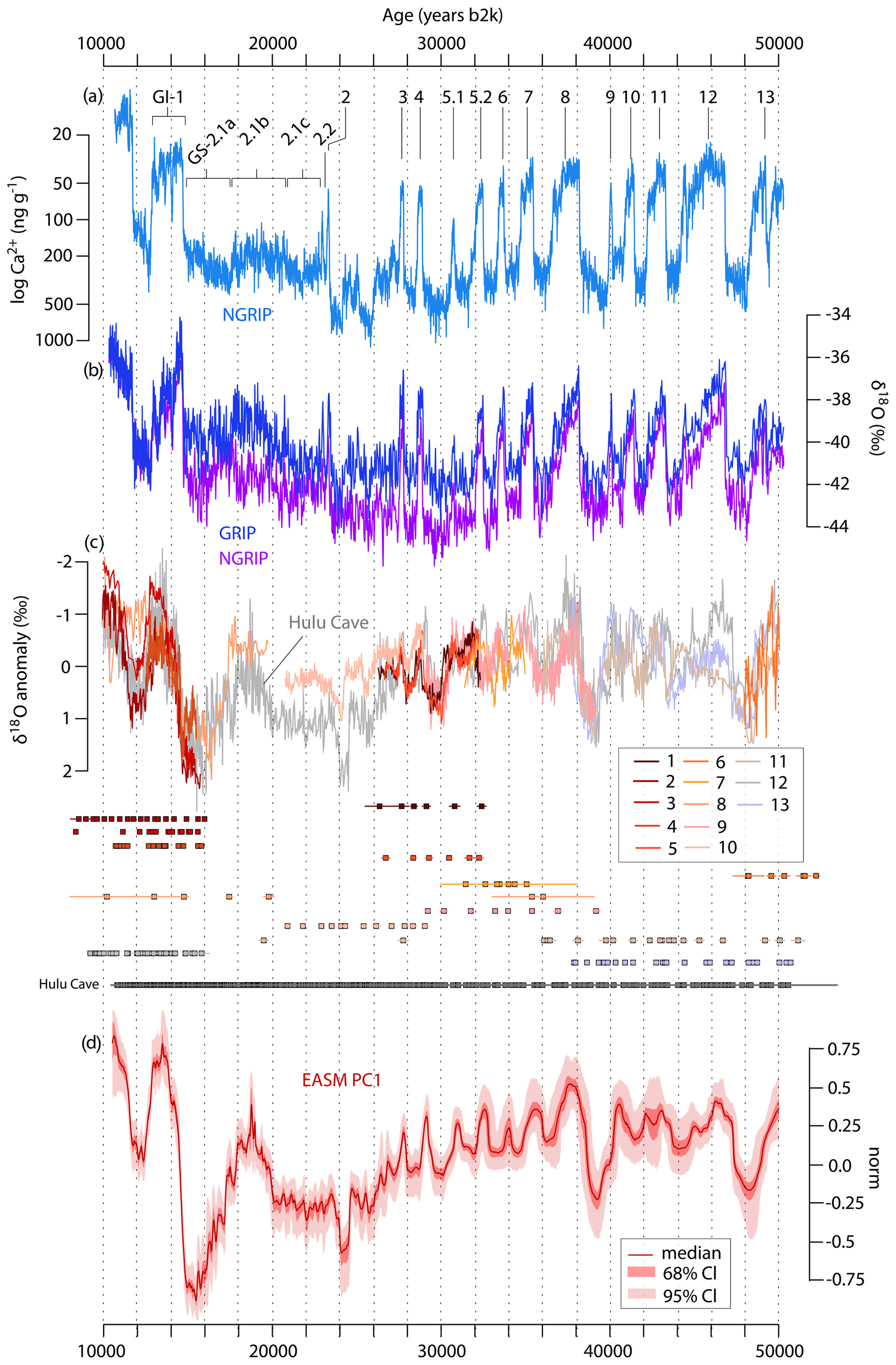
Figure 2 Proxy climate data used for the synchronizations presented in this study and shown on their original timescale. (a) Mineral-dust-derived Ca²⁺ ion concentration record from NGRIP (Erhardt et al., 2019) on the GICC05 timescale (Rasmussen et al., 2006; Svensson et al., 2008). Partitioning of Greenland Interstadials (GIs) and Greenland Stadial (GS) 2 is indicated. (b) NGRIP and GRIP δ¹⁸O record (Andersen et al., 2004; Johnsen et al., 1997) also on the GICC05 timescale. (c) Speleothem δ¹⁸O records from the East Asian summer monsoon (EASM) region presented in Corrick et al. (2020) and used in this study. The high-resolution Hulu Cave δ¹⁸O record (H. Cheng et al., 2016, 2021) on its revised U–Th timescale (H. Cheng et al., 2018, 2021) is shown in gray. δ¹⁸O values are expressed as anomalies from the record mean. Individual U–Th measurements associated with each record are also presented with their ±2σ uncertainty. Numbering refers to the location of cave sites shown in Fig. 1b. (d) First principal component (PC1) of the 14 EASM speleothem records presented in (c) from the MCPCA procedure used in this study (see Sect. 2.1 for details). The solid line indicates the median from the 10 000-member ensemble, while shading reflects the empirical 68 % and 95 % confidence intervals from the ensemble.

Mineral dust aerosol in Greenland ice cores reflects both source strength and transport conditions from terrestrial sources and primarily originates from Asian deserts (Svensson et al., 2000). Its emissions are strongly dependent on Asian hydroclimate via concerted shifts in the latitudinal position of the ITCZ and the EASM system (Nagashima et al., 2011; Schiemann et al., 2009). Because NGRIP Ca²⁺ indirectly registers lower-latitude hydroclimate changes mediated by latitudinal migrations of the ITCZ, it is suitable for direct comparison to EASM δ¹⁸O data, which integrate ITCZ-related shifts in monsoon rainfall over East Asia (Wang et al., 2001, 2006) with comparable durations (Fig. 3). In addition, we performed independent alignments using NGRIP and GRIP δ¹⁸O data – an established proxy for Greenland climate – to assess the sensitivity of our synchronization approach and the coherence across different Greenland ice-core proxy records.

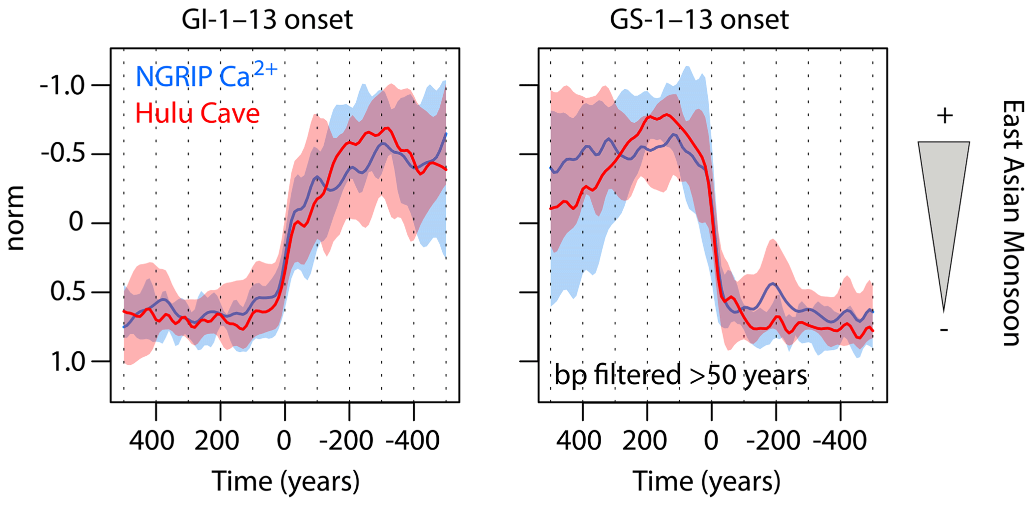
Figure 3 Stack of NGRIP Ca²⁺ and Hulu Cave δ¹⁸ records using a technique in which 13 individual events are centered at the midpoint of their abrupt transition, i.e., either DO warming (onset of GIs) or DO cooling (onset of GSs). The events were normalized and averaged to highlight the shared climatic signal at multidecadal and centennial timescales (>50-year low-pass-filtered) and compare the duration of the abrupt DO transitions between Greenland ice cores and Hulu Cave speleothems. Shading reflects the variability across the events used for stacking. The midpoints of the abrupt transitions were identified using a Bayesian change-point analysis method (Erdman and Emerson, 2007).

As for EASM speleothems, the proxy data are based on a compilation of 14 δ¹⁸O records including the U–Th age determinations underlying each speleothem chronology (Corrick et al., 2020) (Figs. 1a, b and 2b, c). The original compilation included 17 records and we removed 3 low-resolution and scarcely dated records, i.e., whose median age resolution was less than 50 years and had on average less than one U–Th age determination per thousand years. The dataset from Hulu Cave was updated here to incorporate recently published higher-temporal-resolution δ¹⁸O measurements and additional U–Th dates (H. Cheng et al., 2016, 2021). To integrate all the δ¹⁸O data into a single record representative of the EASM region, a Monte Carlo principal component analysis (MCPCA) was used (Fig. 2d). The method follows Anchukaitis and Tierney (2013) and is presented and tested in detail therein. In brief, the procedure allows isolating the common large-scale pattern of hydroclimate variability while accounting for age modeling uncertainties. The MCPCA method uses iterative age modeling of the available U–Th ages and eigen-decomposition of the δ¹⁸O records to produce a reduced set of orthogonal modes that reflect common patterns of δ¹⁸O variability and estimate uncertainties.

In order to perform MCPCA, the different δ¹⁸O records were linearly interpolated to a common time step of 25 years. For this study 10 000 iterations of the MCPCA procedure were generated. In line with Anchukaitis and Tierney (2013), each Monte Carlo iteration consists of the following steps: (1) the U–Th dates of each speleothem record are randomly resampled within their probability distribution imposing that depositional ages increase monotonically with depth; (2) for each record an age–depth model is fit to the resampled U–Th ages using a monotonic piecewise cubic hermite spline; (3) the leading PCA mode (PC1) of the 14 δ¹⁸O proxy records is calculated using probabilistic PCA (Tipping and Bishop, 1999) and ensuring that the sign of the eigenvector is consistent across iterations. The resulting 10 000 ensemble members of the PC1 were used to estimate median and confidence levels, which were ultimately employed as a target record for the synchronization method described below (hereafter referred to as EASM PC1).

2.1.1 Probabilistic algorithm for proxy data synchronization

As discussed in Sect. 1, tie-point and wiggle-matching synchronizations have inherent problems that limit estimating the alignment of proxy time series in a continuous fashion. Although tie-point synchronization is an established and conservative approach, its alignment uncertainty is poorly characterized, tie points can be difficult to reproduce, and even when they are defined statistically the synchronization still does not account for potential shared signal structures in between consecutive ties.

Probabilistic alignment methods have a unique and underexploited potential to correlate proxy time series and move away from pointwise and wiggle-matching synchronization techniques. They are especially well suited for establishing continuous alignments and can help match previously untapped common structures in the signal of climate and cosmogenic radionuclide records. These methods are fully automated and have the advantage of ensuring reproducibility, deriving credible bands associated with the alignment process, and inferring the probability of synchronization solutions based on prior constraints on accumulation rates (e.g., Lin et al., 2014; Muschitiello et al., 2020; Parrenin et al., 2015).

In this study, a continuous synchronization of the GICC05 to the U–Th timescale is established using an appositely developed automated algorithm for probabilistic inversion. The inverse problem is formulated using a Bayesian framework in order to sample the full range of possible GICC05–U–Th synchronization scenarios and explicitly builds in prior ice-core chronological constraints. Assuming that the U–Th timescale is absolute, our inverse scheme simulates the age offset history between GICC05 and the EASM PC1 (i.e., see Sect. 2.1) in response to changes in compaction versus expansion of the Greenland ice-core timescale. The link requires a likelihood function, which quantifies how probable the alignment between ice-core and speleothem records is given a particular simulated ice-layer miscount history.

The numerical approach builds upon previous work using a hidden Markov model for automated synchronization of paleoclimate records (Cutmore et al., 2021; Muschitiello et al., 2019, 2020; Sessford et al., 2019; West et al., 2019, 2021). The model employed here uses constraints imposed by the MCE, i.e., the accumulated absolute annual-layer counting error of the Greenland ice-core chronology, to deform the entirety of an input time series (on the GICC05 timescale) onto a target (on the U–Th timescale). The method minimizes the misfit between the input and the target and finds a sample of alignments between Greenland ice cores and the EASM PC1 record that are physically coherent with the absolute dating uncertainty of GICC05 and some of its counting error properties. However, it should be borne in mind that the model used in this study does not provide a fully comprehensive representation of the complexity that characterizes the ice-core layer counting procedure and its uncertainty (Rasmussen et al., 2006; Svensson et al., 2006). Rather, our approach aims at approximating the counting structure of GICC05 in order to infer estimates of the synchronization uncertainty. The method is also adaptable to a variety of formulations of the inverse problem and to using multiple input and target records simultaneously when determining the alignment.

2.1.2 Inverse modeling approach

In order to establish a continuous alignment between the GICC05 and U–Th timescale, we need to define an alignment function, which relates the GICC05 age of the given input ice-core record (i.e., NGRIP Ca²⁺, NGRIP δ¹⁸O, or GRIP δ¹⁸O) to unknown U–Th ages associated with the target EASM PC1 record. The function is defined here by a mathematical representation of the GICC05–U–Th age relationship that effectively allows linearly stretching and compressing the ice-core chronology relative to the U–Th timescale. To estimate this alignment function, we propose a piecewise linear function (τ(⋅)) with K equally spaced sections within the domain, where the slopes at each section are m_i>0 (note that the slopes, unlike other parameters in the model which are expressed in years, are dimensionless). This ensures no time reversals by guaranteeing that the function is monotonically increasing. The function is also influenced by the initial shift of the alignment. If τ(⋅) represents the alignment function, this initial shift can be defined a τ₀=τ(t₀). Hence, the parameters of τ(⋅) are defined as (τ₀,m), where m is a K-dimensional vector containing the slopes of each evenly spaced section. The model can then be expressed as

$$\begin{array}{}\text{(1)}& \mathit{\tau }\left(t\right)={\mathit{\tau }}_{\mathrm{0}}+\sum _{i=\mathrm{1}}^j\left(m_j\mathrm{\Delta }c\right)+m_{i+\mathrm{1}}\left(t-c_i\right),\end{array}$$

where $c_i\le t<c_{i+\mathrm{1}}$, $\le i<K$, and $c_{\mathrm{0}}<c_{\mathrm{1}}<\mathrm{\cdots }<c_K$ represent evenly spaced time intervals along the GICC05 timeline with length Δc. The slopes $m=(m_{\mathrm{1}},m_{\mathrm{2}},\mathrm{\dots },m_K)$ correspond to the linear sections within each interval. This function is analogous to the one employed to construct age–depth models (Blaauw and Christen, 2011), i.e., a piecewise linear function with positive slopes, which prevents time reversals but preserves the shifts (m_jΔc) from younger to older sections. It is important to note that the piecewise linear technique adopted here provides a key advantage compared to a simple global linear function in its ability to accommodate local variations, i.e., approximating the nonlinear nature of the alignment. While a linear model imposes a single linear trend across the entire dataset, the piecewise linear model allows for different shorter linear behaviors within each segment, thereby providing a more nuanced and accurate representation of the alignment. The parameter space created by the piecewise linear model is of size K+2. This structure facilitates effective posterior exploration and global optimization as it offers control over the model's parameterization and allows users to adjust its flexibility. This balance enables a thorough yet efficient examination of the parameter space, ensuring the optimal selection of the number of parameters without the computational complexity and overfitting risks associated with a larger number of sections.

However, it should be noted that our proposed method for calculating the alignment function, τ(t), significantly differs from the one presented by Blaauw and Christen (2011), which employs an autoregressive gamma process for simulating sedimentation rates with downcore dependence. Unlike their method, ours restricts such information exchange, thereby preserving the independence of each section. This feature is suitable given our data context, which underlie very different proxy measurements. It is important to note that since the input and target records are provided on their own independent chronologies, we do not need to model the autocorrelation associated with each timescale. Therefore, our approach, which maintains the independence of each section, is better suited for these datasets.

Our goal is to deploy a method for inferring the alignment function τ(t), which minimizes the misfit between the ice-core data on the GICC05 timescale t^′ and the EASM PC1 on the U–Th timescale t. Let us define the ith data point in the input ice-core record associated with time $t_i^{\prime }$ on the GICC05 timescale as g_i. Therefore, the vector g denotes the input signal, containing the NGRIP Ca²⁺, NGRIP δ¹⁸O, or GRIP δ¹⁸O measurements on the GICC05 timescale. Analogously, for the EASM PC1 record, each data point, defined as u_j, represents the target signal at time t_j on the U–Th timescale. The vector u houses this target signal and contains the data from the EASM PC1 record on the U–Th timescale.

With this notation, we regard each datum in u and g as an observation of the proxy at a specific point in time (t_i), following a normal distribution where the mean corresponds to the “true” value of the proxy at time t_i (U and G). In this case, the input record is reported without errors, so it can be assumed that G=g. On the other hand, the target record is accompanied by uncertainty (${\mathit{\sigma }}_{u_i}^{\mathrm{2}}$), so we assume $u_i\sim N(U_i,{\mathit{\sigma }}_{u_i}^{\mathrm{2}})$, where ${\mathit{\sigma }}_{u_i}^{\mathrm{2}}$ denotes the variance of each data point u_i. It should be noted that u_j is associated with a time t_i, and thus the appropriate notation is u_j(t_i). Assuming that both the input and target are adequately synchronized by the alignment function τ(t), $\forall u\left(t_i\right)\approx g\left(\mathit{\tau }\right(t_i\left)\right),t_i\in \mathit{t}$ holds true. It should be borne in mind that this assumption does not imply a perfect fit between u and g, but rather the existence of a τ(t) that maximizes the similarity across the whole records. To evaluate the goodness of the fit between u and g, and given that the uncertainty associated with u can be considered a random variable, here we use the approach devised by Christen and Pérez (2009). Accordingly, we define u_i as follows:

$$\begin{array}{}\text{(2)}& u_i|{\mathit{\tau }}_{\mathrm{0}},m,t_i,\mathit{G},{\mathit{\sigma }}_{u_i}^{\mathrm{2}}\sim t\left(G\left(\mathit{\tau }\left(t_i\right)\right),{\mathit{\sigma }}_{u_i}^{\mathrm{2}},a,b\right),\end{array}$$

where a and b are the parameters of the t distribution (Christen and Pérez, 2009). It is important to stress that G is set only at discrete times, t^′, which may not necessarily match an observed U–Th age on the target EASM PC1 record (t). To obtain values for G(τ(t_i)) at any specific time, we employ linear interpolation using the observations from GICC05. This method enables us to compute G(t) for any given $t\in (t_{\mathrm{0}}^{\prime },t_m^{\prime })$, where ($t_{\mathrm{0}}^{\prime },t_m^{\prime }$) is the time window of the input ice-core record on the GICC05 timescale, whereby $t_{\mathrm{0}}^{\prime }=\mathrm{10.75}$ kyr b2k and $t_m^{\prime }=\mathrm{48}$ kyr b2k. Finally, it is also important to note that before synchronization, the input and target records are scaled between −1 and 1. Despite the potential for scaling to introduce alignment biases when dealing with outliers or extreme maxima and/or minima, our synchronization method employs a continuous function with constraints on the stretching and compression of the input (see Sect. 2.2.3). This approach addresses potential mismatches by considering the overall structure of the data and the assumption of continuity. Moreover, our methodology quantifies the alignment uncertainty by evaluating the quality across the entire record, accounting for the inherent uncertainty in aligning all of the data, ensuring reliable synchronization. Finally, the uncertainty of the target is assigned an overly conservative value of 0.2, and bearing in mind that we allow for a heavy tailed t-distribution error, this effectively ensures covering 60 % of the observable window in the data. By overestimating the variance of the input, we thus augment the model's ability to identify similarities between the target and input, especially over intervals with a clear offset between the two datasets.

2.1.3 Model's likelihood, parameters, and priors

Since the synchronization process is fundamentally uncertain, we apply a Bayesian approach to infer the optimal alignment between u and g that accounts for glaciological information on unobserved changes in the annual-layer miscount of Greenland ice cores. For the correct implementation of this approach we require a likelihood function. This likelihood function evaluates the previously mentioned assumption (U(t_i)≈G(τ(t_i))) of the aligned ice-core record and the target speleothem data given a particular set of parameter values $\mathrm{\Phi }=({\mathit{\tau }}_{\mathrm{0}},m,\mathit{G},{\mathit{\sigma }}_{u_i}^{\mathrm{2}})$. The model is defined by Eq. (3), which allow us to calculate the log-likelihood of the data as

$$\begin{array}{}\text{(3)}& l\propto \sum _{i=\mathrm{0}}^n\left[-\log \left({\mathit{\sigma }}_{u_i}\right)-{\displaystyle \frac{a}{\mathrm{2}}}\log \left(b+{\displaystyle \frac{{\left(G\mathit{\tau }\left(t_i\right)-u_i\right)}^{\mathrm{2}}}{\mathrm{2}{\mathit{\sigma }}_{u_i}^{\mathrm{2}}}}\right)\right].\end{array}$$

In the synchronization problem posed here, the likelihood function determines the goodness of the fit by minimizing the mismatch between the input and the target at every data point on the U–Th timescale, i.e., by optimizing the function τ(⋅). τ₀ and m are model parameters, whereas G, ${\mathit{\sigma }}_{u_i}^{\mathrm{2}}$, and t_i are related to the data. G refers to the input data on the GICC05 timescale, and ${\mathit{\sigma }}_{u_i}^{\mathrm{2}}$ refers to the reported variance of the target record on the U–Th timescale. To provide a more conservative measure of the uncertainty surrounding G, we use the t distribution (Christen and Pérez, 2009). Lastly, t_i represents the time of the ith target signal on the U–Th timescale.

The model estimates the probability of a given alignment that relates GICC05 and U–Th ages by evaluating the log-likelihood function described in Eq. (3) together with prior distributions for τ₀ and m. To avoid sampling outside a physically reasonable range and to identify a sample of optimal synchronizations, this probability is based on prior knowledge that the alignment between the input and target is largely limited by the constraints imposed by the absolute counting error of GICC05. Given that the parameters τ₀ and m are largely unknown and must be inferred from the model, we assign uninformative priors to ensure that the posterior alignment is mainly influenced by the data. For τ₀, which defines the initial timescale offset at time t₀, we apply a prior distribution of ${\mathit{\tau }}_{\mathrm{0}}\sim {\mathrm{1}}_{(-\mathrm{MCE}<m_i<\mathrm{MCE})}N(t_{\mathrm{0}},{\mathit{\sigma }}_{\mathrm{0}})$, where ${\mathit{\sigma }}_{\mathrm{0}}=\frac{\mathrm{MCE}}{\mathrm{2}}$, and MCE is the maximum counting error of GICC05 at t₀.

Since one of the objectives of this study is to infer changes in the GICC05–U–Th timescale difference (hereafter expressed as $\mathrm{\Delta }T=t^{\prime }-t$), we invert the relative counting error (RCE) of GICC05, which is defined as the rate of change of the MCE. The decision to use RCE is justified because it reflects the speed at which the counting error changes, thus making it a suitable metric for constraining the slopes of the function τ. To account for changes in ΔT brought about by possible unaccounted biases in the ice-core annual-layer counting, the prior knowledge should allow sampling an RCE greater than the nominal values imposed by the GICC05, which during the last glacial period range ∼5 %–10 % (Svensson et al., 2006, 2008). In our model, each slope within the vector m is independent and strictly positive. The slopes reflect the rate at which the age relationship between the GICC05 and U–Th timescales changes over two adjacent sections, whereby m_i>1 implies a linear stretching of GICC05, and $\mathrm{0}>m_i>\mathrm{1}$ implies a compression. With this understanding, we assigned m_i a truncated normal distribution $m_i\sim {\mathrm{1}}_{(\mathrm{0}<m_i<\mathrm{5}\mathrm{RCE})}N(\mathrm{0},{\mathit{\sigma }}_m^{\mathrm{2}})$, which ensures that m_i remains positive. This effectively allows the model to explore RCE values up to 5 times greater than nominal and consider GICC05–U–Th synchronizations that exceed the range allowed by the MCE, as well as accommodating propagation of the age errors associated with the U–Th timescale. To ensure that m_i follows the GICC05 counting error, ${\mathit{\sigma }}_m^{\mathrm{2}}$ is fixed to be half the RCE at a given time t. In our implementation, we have set the value of K to 200, which implies that the time span of U(t_i) is divided into 200 sections (i.e., ∼180 years per section). This division provides a reasonable compromise between computational performance and alignment resolution, ensuring that each section contains enough data for meaningful results.

In order to calculate a posterior sample of the parameters and optimize the function τ(⋅), a Markov chain Monte Carlo methodology is used (see Sect. 2.2.4). This approach not only aims to find the best parameter values but also generates samples of the posterior distributions for each parameter. These samples are valuable for inferring credible intervals related to the alignment and can even be utilized to propagate the latter into the aligned proxies.

2.1.4 MCMC: determining the posterior distribution

Because of the nonlinear nature of the synchronization problem and the fact that there are far too many alignments to calculate all their probabilities, a stochastic Monte Carlo method is required to explore the posterior distribution in a computationally efficient way. Calculation of the posterior probability proceeds by sampling an initial value for each unknown model parameter from the associated prior distributions using Markov chain Monte Carlo (MCMC). MCMC techniques play a key role in statistical analysis, providing a systematic method for sampling from complex, multidimensional posterior distributions. The principles of MCMC algorithms are based on the concept of a Markov chain, where the future state solely depends on the current state, not on the series of previous states. Beginning from an arbitrary point, the MCMC algorithm initiates a sequence of steps or “leaps” across the parameter space. The direction and magnitude of each leap are governed by a set of predefined rules specific to each MCMC method. Over time, this sequence of leaps effectively samples the target distribution. Regardless of where it starts, the algorithm ensures that it will converge to and accurately sample from the target distribution, provided it completes enough iterations (Brooks et al., 2011). The time or number of iterations required for the algorithm to stabilize and accurately reflect the posterior distribution is commonly referred to as the “burn-in” period. This convergence is what allows us to obtain accurate samples from the posterior distribution, enabling us to infer the model's parameters.

In this study, MCMC is driven by a differential evolution Markov chain (DE-MCz) sampler (Ter Braak and Vrugt, 2008), which is particularly effective in dealing with multi-modal posterior probability distributions. The DE-MCZ method is designed to update various segments of the Markov chain simultaneously, which significantly speeds up the processing time for large multidimensional datasets. Additionally, DE-MCz's inherent adaptability makes it an excellent choice for tackling complex problems and an ideal MCMC for our implementation.

The sampler was run for 1.5×10⁶ MCMC iterations after disregarding a burn-in time of 0.5×10⁶ steps and only retaining every 10th iteration to mitigate the statistical dependence of the model parameters. This was deemed to be a sufficiently long MCMC run for the simulation to reach convergence, as monitored by a multivariate potential scale reduction factor less than 1.1 (Brooks and Gelman, 1998). The sample from the remaining iterations was used to estimate the posterior distribution of each random variable in the model (τ₀ and m). By leveraging samples from these parameters, we computed a posterior sample of alignment functions τ(⋅). This posterior sample of functions then allows us to evaluate metrics such as the median and credibility intervals. However, note that this is a simplification of the process behind it: because the resulting output is a sample of random variables, the most appropriate way to report these results is the ensemble of samples from τ(⋅). Nevertheless, in order to simplify the output and follow common practice, we reported the median and 95 % credible intervals.

3 Results and discussion

3.1 Synchronization and timescale transfer functions

The leading mode of the MCPCA procedure – i.e., the EASM PC1 – provides the target record for the CLIM synchronizations and is presented in Fig. 2d. The PC1 is dominated by the characteristic EASM hydroclimate signal, and even though the Monte Carlo approach results in some temporal smoothing, the millennial-scale trends and shorter events that punctuated the last glacial period in this region are reasonably well captured. The Hulu Cave record has the largest loading on PC1 as it is the dataset with the highest temporal resolution and the only one stretching over the whole synchronization interval. It loads highly especially between ∼16 and 28 kyr b2k where there are fewer speleothem records.

The inverted CLIM synchronizations and related GICC05–U–Th timescale transfer functions are presented in Figs. 4–6. Before we interpret the timescale transfer functions, a consideration should be made. As outlined in Sect. 2.2, the entirety of the input and the target are scaled between −1 and 1 before synchronization. This scaling may introduce a systematic alignment bias when either the input or target features extreme maxima or minima, as these will affect the structure of the records by introducing artificial trends. To test for the sensitivity to scaling, we conducted additional synchronization experiments on NGRIP δ¹⁸O by performing localized alignments against the EASM PC1 using shorter intervals of ∼10 kyr and after scaling the input and target segments (Fig. S1 in the Supplement). These sensitivity tests reveal that the localized and global alignments are largely coherent throughout the interval ∼11–48 kyr b2k and thus support the robustness of our approach. More importantly, they highlight the advantage of estimating a global alignment, whereby the synchronization uncertainty is estimated by jointly considering all the linear sections of the input and target and their respective errors.

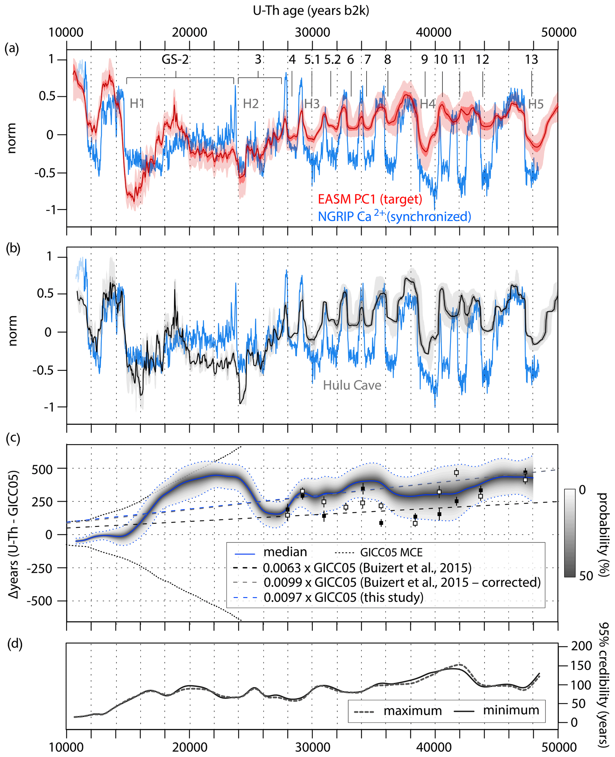
Figure 4 CLIM1 synchronization of GICC05 to the U–Th timescale and resulting timescale transfer function. (a) Synchronized NGRIP Ca²⁺ data on the U–Th timescale using the posterior median estimate of the MCMC synchronization. The synchronization was derived from stratigraphic alignment of the NGRIP Ca²⁺ data to the East Asian summer monsoon (EASM) PC1 (see Sect. 2.1 for details). Shading reflects the empirical 68 % and 95 % confidence intervals from the 10 000-member ensemble. Greenland Stadials (GSs) and the timing of Heinrich events (H) are indicated at the top. (b) Comparison between the synchronized ice-core data and the Hulu Cave δ¹⁸O record with its associated age uncertainty (gray shading: light, 68 %; dark, 95 %). All proxy records are shown in normalized units. (c) Posterior median (blue continuous line) and pointwise 95 % credible intervals (shading and blue dashed lines) of the difference ΔT between the GICC05 and U–Th timescales. The black squares are the Hulu–NGRIP age offsets presented in Buizert et al  (2015), and the white squares reflect the same offsets corrected using the updated U–Th chronology presented in Cheng et al. (2018). The corrected offsets were estimated using a cross-correlation analysis of the Hulu Cave δ¹⁸O data on the previous and the latest timescale, respectively (Fig. S2). The linear fit through these data and that estimated from our ΔT values are also shown. Note that the linear models are forced to intersect the origin. (d) Posterior credible intervals of the transfer function shown in (c). Gray dashed and black lines reflect the maximum and minimum bound of the credible intervals, respectively.

Figure 5 Same as Fig. 4 but for CLIM2, i.e., using NGRIP δ¹⁸O data.

Figure 6 Same as Fig. 4 but for CLIM3, i.e., using GRIP δ¹⁸O data.

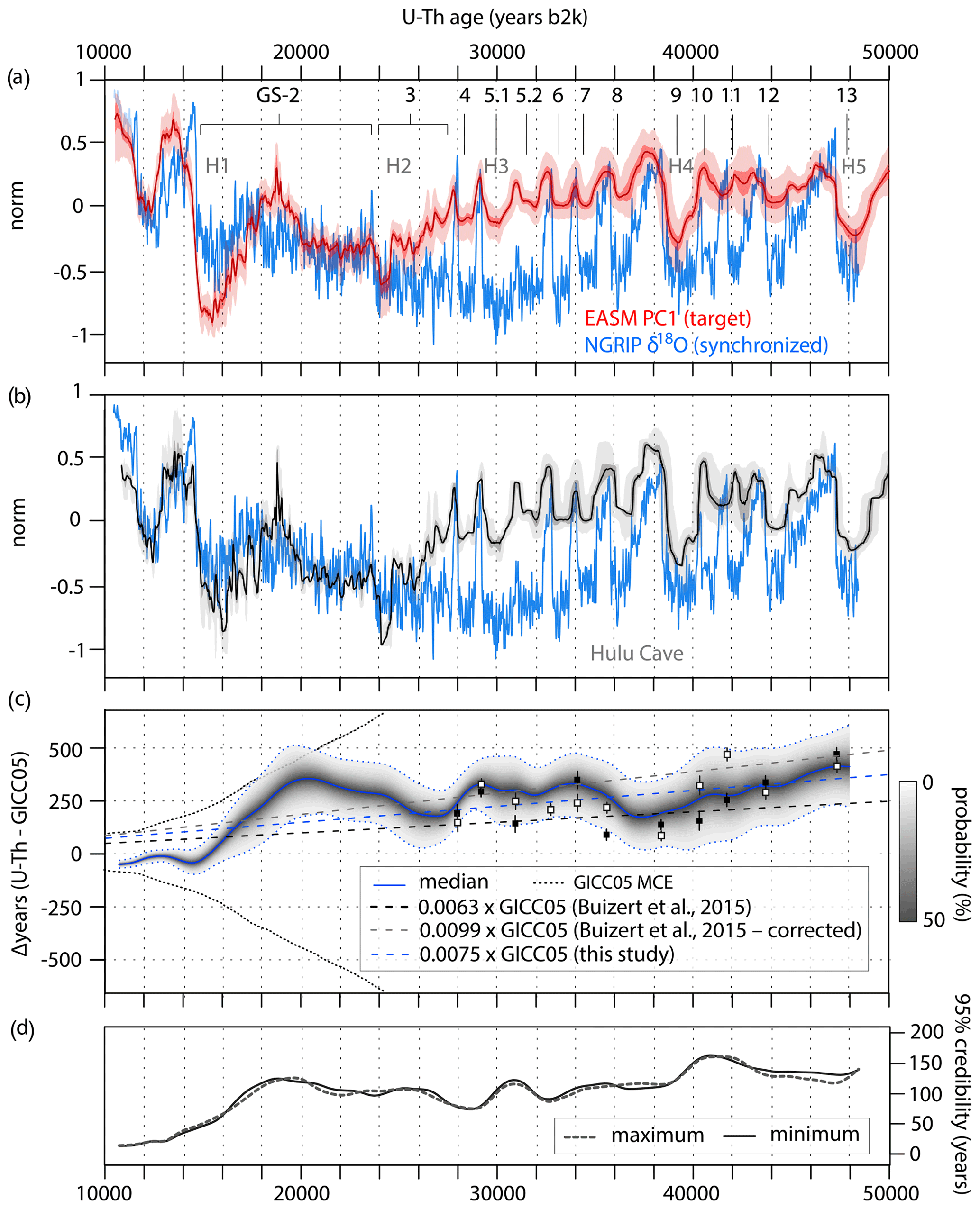
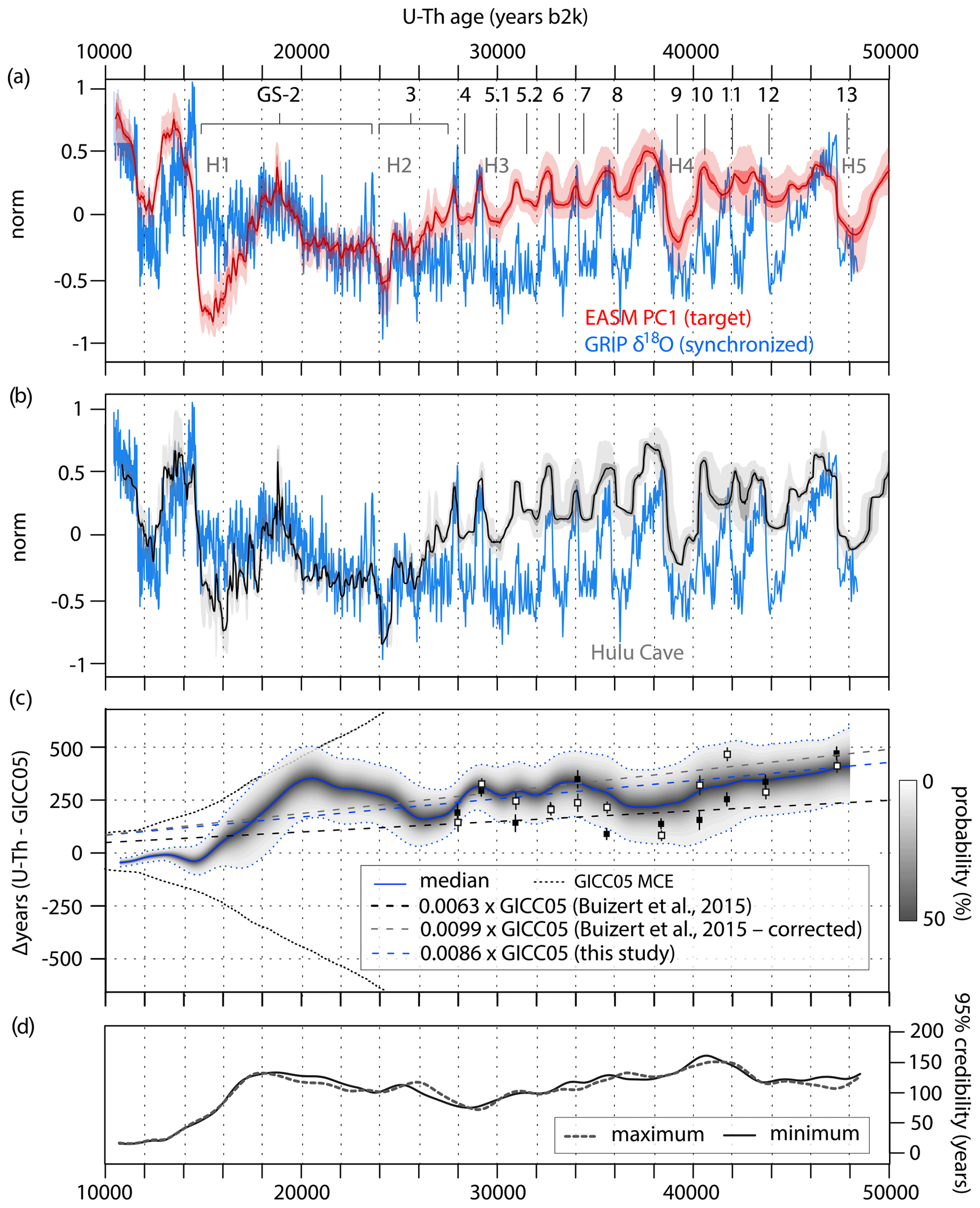
Assuming that our methodological approach is adequate, that the U–Th timescale is accurate and considering the age uncertainties associated with EASM PC1, it can be observed that throughout the last glacial period the timescale difference ΔT is well within the MCE limits of GICC05. Notably, GICC05 is systematically younger than the U–Th timescale and the age difference increases with time, indicating, on average, a stretch of 0.97 % for CLIM1, 0.75 % for CLIM2, and 0.86 % for CLIM3 (mean = 0.86 %) during the construction of GICC05, which is comparable to the 0.99 % linear scaling bias estimated by Buizert et al. (2015) after correcting for the new U–Th chronology presented in Cheng et al. (2018) (Fig. S2).

The CLIM synchronizations are broadly coherent, and superimposed upon this upward trend there are a number of consistent shorter-term ΔT fluctuations. The CLIM results indicate that at the onset of the Holocene, GICC05 is slightly older than the U–Th timescale, yielding a consistent ΔT of $-{\mathrm{45}}_{-\mathrm{65}}^{-\mathrm{25}}$ years (95 % credible range) for CLIM1 (Fig. 4c), $-{\mathrm{45}}_{-\mathrm{55}}^{-\mathrm{30}}$ years for CLIM2 (Fig. 5c), and $-{\mathrm{45}}_{-\mathrm{55}}^{-\mathrm{30}}$ years for CLIM3 (Fig. 6c), which is remarkably similar to previous independent estimates based on correlation of ¹⁴C and ¹⁰Be records (i.e., −65 years; Muscheler et al., 2008). In the interval ∼15–24 kyr b2k, corresponding to the early stage of GS-2, GICC05 is steadily stretched faster than allowed by the annual counting error, reaching a maximum ΔT between ∼20 and 22 kyr b2k of $+{\mathrm{450}}_{+\mathrm{355}}^{+\mathrm{550}}$ years for CLIM1, $+{\mathrm{360}}_{+\mathrm{245}}^{+\mathrm{465}}$ years for CLIM2, and $+{\mathrm{355}}_{+\mathrm{230}}^{+\mathrm{465}}$ years for CLIM3 (mean = ∼390 years), which is as large as or a little larger than the MCE permits. Again, this is in good agreement with recent estimates based on BWM of cosmogenic radionuclides (i.e., 375 years; Sinnl et al., 2023) and climate synchronization (i.e., 320 years; Dong et al., 2022), respectively. From ∼24 to 27 kyr b2k, which corresponds to GS-3 and is approximately in phase with the global LGM ice-volume peak (Hughes and Gibbard, 2015), again the GICC05 annual-layer count changes faster than the counting error allows, highlighting a possible compression of the timescale with ΔT values dropping to $+{\mathrm{160}}_{+\mathrm{55}}^{+\mathrm{250}}$ years for CLIM1, $+{\mathrm{180}}_{+\mathrm{90}}^{+\mathrm{270}}$ years for CLIM2, and $+{\mathrm{160}}_{+\mathrm{70}}^{+\mathrm{270}}$ years for CLIM3 (mean = ∼165 years). Between ∼28 and 29.5 kyr b2k, another short-term stretch of GICC05 is observed, when ΔT values raise to $+{\mathrm{320}}_{+\mathrm{210}}^{+\mathrm{420}}$ years for CLIM1, $+{\mathrm{330}}_{+\mathrm{245}}^{+\mathrm{415}}$ years for CLIM2, and $+{\mathrm{315}}_{+\mathrm{235}}^{+\mathrm{285}}$ years for CLIM3 (mean = ∼320 years). Thereafter, ΔT values exhibit – within the uncertainty bounds – stable and gradually increasing values until 48 kyr b2k, reaching a maximum of $+{\mathrm{430}}_{+\mathrm{250}}^{+\mathrm{600}}$ years for CLIM1, $+{\mathrm{415}}_{+\mathrm{280}}^{+\mathrm{555}}$ years for CLIM2, $+{\mathrm{410}}_{+\mathrm{280}}^{+\mathrm{535}}$ years for CLIM3 (mean = ∼420 years).

The largest ΔT excursions between ∼15 and 28 kyr b2k are primarily controlled by the millennial-scale and shorter-term variability recorded in the Greenland ice-core data and EASM PC1 (Figs. 4a, 5a, and 6a). The overall match is driven by the alignment between the GS-3 dust peaks and coolings in the Greenland ice cores (Rasmussen et al., 2008) and the well-defined declines in monsoon strength observed in EASM PC1, as well as by a few marked proxy excursions during GS-2 (Figs. 4a, 5a, and 6a). However, the transfer function errors are relatively large during GS-2 (Figs. 4d, 5d, and 6d). This is mainly due to the relatively lower signal-to-noise ratio in the climate records across the late glacial and LGM, where the alignment is less robust. In the case of the LGM, further work and independent age constraints would therefore be desirable to improve the match between the GICC05 and U–Th timescales. Before ∼28 kyr b2k, the ΔT results are largely constrained by the match between stadial–interstadial transitions in Greenland ice cores and the corresponding monsoon events integrated in the EASM PC1 (Figs. 4a, 5a, and 6a), with the exception of the interval surrounding GS-10 and GI-10 at ∼42 kyr b2k when the speleothem δ¹⁸O data underpinning the EASM PC1 exhibit some temporal inconsistencies, thus resulting in a larger synchronization error (Figs. 4d, 5d, and 6d).

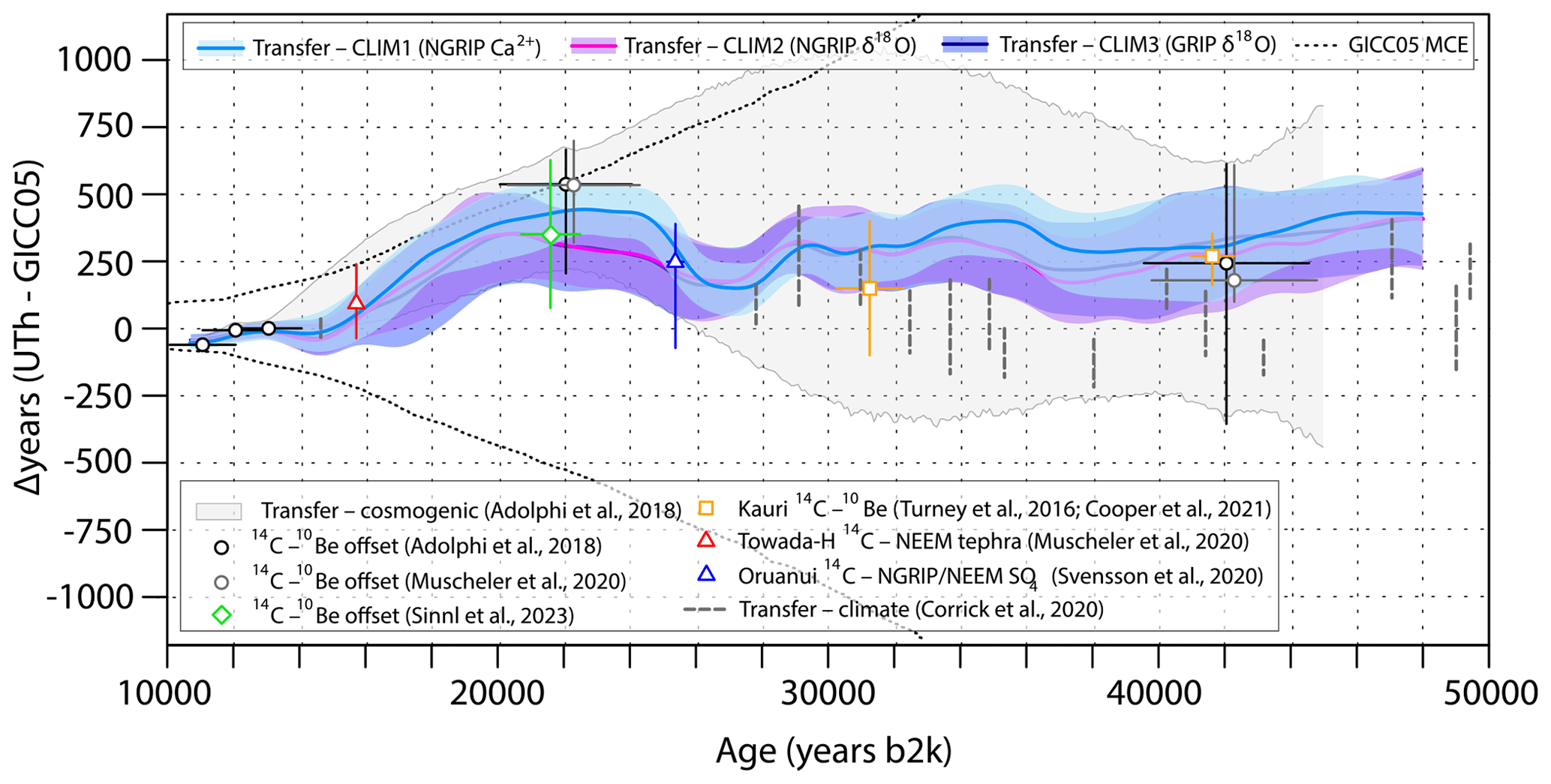
Figure 7 Posterior timescale transfer function based on the CLIM MCMC synchronizations presented in this study. Positive values indicate that the U–Th timescale is older than GICC05. The transfer function is presented with its median (thick lines) and pointwise 95 % credible intervals (shading). The results are compared to the transfer function presented in Adolphi et al. (2018) (gray shading), which is based on a compilation of U–Th-dated ¹⁴C records, including the low-resolution and less precisely dated Hulu Cave data (Southon et al., 2012). The markers with error bars (±2σ) show discrete match points inferred from comparison of ice-core ¹⁰Be records and absolutely dated ¹⁴C data (Adolphi et al., 2018; Cooper et al., 2021; Muscheler et al., 2020; Sinnl et al., 2023; Turney et al., 2016), ¹⁴C-dated volcanic eruptions identified in Greenland ice cores (Muscheler et al., 2020; Svensson et al., 2020), and climate tie points (Corrick et al., 2020). The dashed lines highlight the maximum counting uncertainty of GICC05.

A comparison of the CLIM timescale transfer functions alongside published ΔT estimates is presented in Fig. 7. The inferred timescale offset history is in good agreement with independent ΔT estimates based on BWM of cosmogenic radionuclide records and match points between GICC05 and the ¹⁴C timescale. The uncertainty bounds are overall ∼52 % narrower than previous estimates based on BWM (Adolphi et al., 2018; Muscheler et al., 2020) for CLIM1, ∼47 % for CLIM2, and ∼45 % for CLIM3 (mean = 48 %). Uncertainties are on average ∼30 % smaller during deglaciation and LGM (i.e., after 28 kyr b2k) for CLIM1, ∼24 % for CLIM2, and ∼19 % for CLIM3 (mean = 24 %), whereas the precision is improved by up to ∼73 % during Marine Isotope Stage 3 (i.e., prior to 28 kyr b2k) for CLIM1, ∼70 % for CLIM2, and ∼70 % for CLIM3 (mean = 71 %).

It is interesting to note that, during the interval 32–40 kyr b2k, we did not find a compelling match with the ΔT estimates based on climate tie points presented in Corrick et al. (2020). These tie points are also systematically different from the cosmogenic radionuclide ΔT values and the scaling bias estimated by Buizert et al. (2015). Corrick et al. (2020) suggested that such mismatch may stem from their methodological approach, including the application of a revised detrital thorium correction to U–Th dates and/or their depth–age modeling procedure. Additionally, and more fundamentally, Corrick et al. relied on visual identification of the abrupt climate transitions in speleothem δ¹⁸O that involved different degrees of subjectivity. This is in contrast with our methodology as well as the statistical approaches adopted for BWM of cosmogenic radionuclides and identification of the match points presented in Buizert et al. (2015), respectively. We hope that these considerations will stimulate further work to reconsider and reconcile these age discrepancies.

In conclusion, not only are the new timescale transfer functions considerably more precise, but the continuous synchronization also brings to light a more complex GICC05–U–Th age difference history than previously assumed. Moreover, our synchronization model allowed identifying a number of potential fast changes in the timescale difference – i.e., features that would have gone undetected had the model been more tightly constrained by the nominal RCE of GICC05.

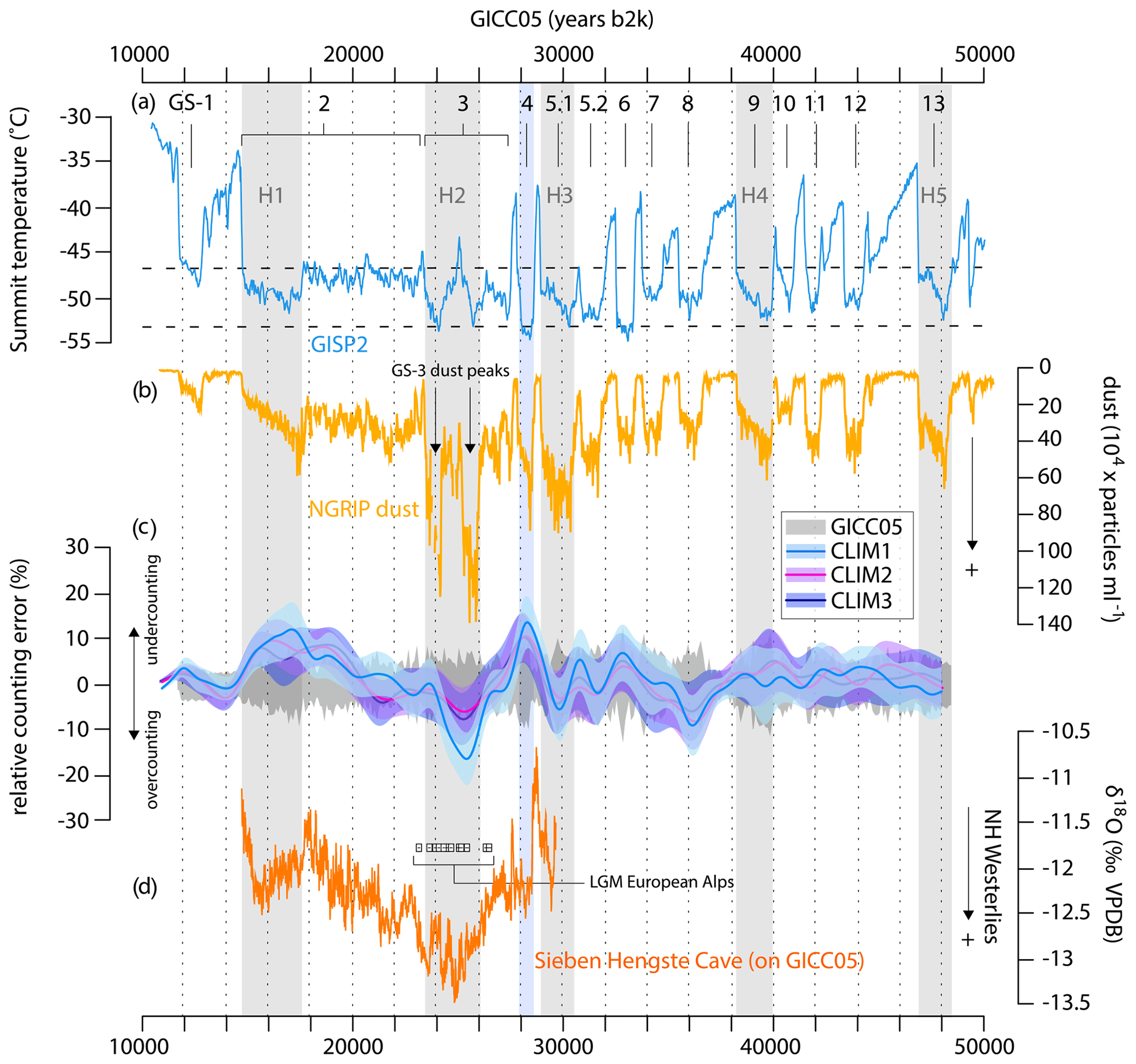
Figure 8 Inferred estimates of the relative annual-layer counting error for the GICC05 chronology based on MCMC synchronization to the U–Th timescale. (a) GISP2 temperature reconstruction (Martin et al., 2023) presented with partitioning of Greenland Stadials (GSs) and the timing of Heinrich events (H; gray vertical bars). Underlying dashed levels show the ±2σ temperature range of stadials GS-1 to GS-13. Interstadial–stadial transitions were identified using a Bayesian change-point procedure (Erdman and Emerson, 2007). The blue vertical bar denotes GS-4, i.e., the coldest stadial (∼3.3 °C colder than the average). (b) NGRIP insoluble dust concentration record (Ruth et al., 2003) (note the reverse scale). (c) Comparison between the maximum relative counting error of the GICC05 (gray shading) and the differential dating uncertainties inferred from the CLIM synchronizations presented in this study, respectively, shown with their posterior median (thick lines) and pointwise 68 % credible intervals (shading). Positive (negative) values indicate an undercount (overcount) of ice layers in Greenland ice cores. To emphasize the longer-timescale variance, the data are smoothed to remove variability shorter than 2000 years. (d) U–Th dated climate records of the Last Glacial Maximum (LGM) in the European Alps after synchronization to the GICC05 timescale by applying the CLIM1 transfer function presented in this study. U–Th ages of cryogenic cave carbonates (Spötl et al., 2021) with their ±2σ uncertainty (white squares) indicating the timing of the maximum mountain glacier extent over the European Alps and δ¹⁸O values of precipitation from the Sieben Hengste stalagmite record (Luetscher et al., 2015) (orange). The Sieben Hengste record reveals a maximum strengthening and southerly displacement of the westerly winds during GS-3. All records are presented on the GICC05 timescale.

3.2 Differential dating uncertainty of GICC05

It should be noted that a major assumption of our methodology is that the U–Th timescale is reliable. While this is certainly reasonable, the timescale may be problematic in certain intervals such as between ∼40 and 44 kyr b2k (Fig. 2c and d), and results over this period should therefore be treated with caution. Assuming that the U–Th timescale is absolute outside this brief interval, a new picture emerges showing that the identification of uncertain annual layers in the GICC05 is potentially less accurate than previously thought (Figs. 7 and 8). The GICC05 timescale appears to be either missing or gaining time beyond its RCE during some of the longest and coldest stadials (Fig. 8). Most notably, too few annual layers have been identified within H1/GS-2 and GS-4, whereas too many layers have been counted over H2/GS-3, i.e., the LGM. In principle, these results – which are largely consistent across the three CLIM synchronizations – challenge the layer counting method and uncertainty estimates and imply that the bias in the GICC05 layer counting does not systematically depend on accumulation rates.

The observation that GICC05 likely undercounts ice layers during H1/GS-2 is quantitatively comparable to previous results based on BWM of cosmogenic radionuclides (Adolphi et al., 2018; Sinnl et al., 2023) (Fig. 7) and recent estimates based on climate synchronization (Dong et al., 2022). Specifically, the synchronizations highlight that GICC05 counts on average ∼12 % too few annual layers in the interval ∼15–18 kyr b2k for CLIM1, ∼10 % for CLIM2, and ∼9 % for CLIM3 (mean = ∼10 %). Similarly, during GS-4, which represents the coldest period recorded in Greenland ice cores (Fig. 8a), we observe an undercount of ∼14 % centered at ∼28 kyr b2k for CLIM1, ∼12 % for CLIM2, and ∼12 % for CLIM3 (mean = ∼13 %).

Perhaps a more interesting result is that throughout most of LGM/GS-3 there is an increasing tendency to count too many years in the GICC05 stratigraphy, which is particularly evident in CLIM1. The overcount starts at ∼24 kyr b2k and reaches a maximum rate of change at ∼26 kyr b2k, when the GICC05 timescale counts on average ∼16 % too many layers (Fig. 8c). This is less pronounced in CLIM2 and CLIM3 but still evident, indicating an overcount of ∼6 % and ∼9 %, respectively (mean = ∼10 %). The LGM/GS-3 interval is one of the coldest sections of the last glacial period (Fig. 8a and b) and an overcount of annual layers is seemingly at odds with the general assumption that fewer years have been detected during stadials, i.e., when low accumulation rates and thinner ice layers make the identification of annual layers more difficult (Rasmussen et al., 2006; Svensson et al., 2006, 2008). However, a bias towards counting too many ice years during LGM/GS-3 is not unexpected as there are some weak indications that additional annual layers have been counted in other cold sections of the GICC05 stratigraphy (Andersen et al., 2006; Rasmussen et al., 2006; Svensson et al., 2006).

This finding requires further consideration. During LGM/GS-3, the RCE inferred from CLIM maps onto the dust concentration profile in Greenland ice cores (Fig. 8b and c). This interval features the two most distinct and pronounced dust peaks of the last glacial period, in which dust levels increase by a factor of 3 in NGRIP ice cores (Ruth et al., 2003). Since high dust content in the ice is notoriously liable to complicate the annual-layer counting in a number of ways, this correspondence suggests a possible impact of dust deposition on the identification of the annual layers.

The layer counting in the coldest climatic events of the GICC05 stratigraphy relies mostly on the visual identification of annual variations in two parameters over the NGRIP ice cores. Since the chemical records do not resolve the thin stadial layers, counting is constrained using the high-resolution visual stratigraphy (VS) grayscale refraction profile (Svensson et al., 2005) and the electrical conductivity measurement (ECM) on the solid ice (Dahl-Jensen et al., 2002; Hammer, 1980). The VS profile represents the depositional history at NGRIP. Inspections of the VS data throughout the glacial period highlights a strong correlation between the frequency of visible layers and dust concentration, suggesting that the intensity (i.e., the gray value) of each layer is related to its impurity content representing an individual dust depositional event (Svensson et al., 2005). This may result in the VS record containing multiple visible large layers per year, which can complicate the counting and lead to a misinterpretation of the actual annual signal. On the other hand, the ECM is strongly dominated by variations in dust (e.g., Taylor et al., 1997). The ECM profile is attenuated in sections with high concentrations of dust due to the increased alkalinity, thus subduing the annual cycle in the ECM signal and making the resolution of this parameter marginal for the identification of annual layers (Andersen et al., 2006; Rasmussen et al., 2008). For these reasons, greater dust deposition rates may limit the use of the VS and ECM data for direct counting of annual layers.

Moreover, accurate counting over the cold sections that feature multiple depositional events depends on the untested assumption that clusters of peaks in the VS and ECM profiles reflect seasonal variations in dust deposition resembling those observed in the shallower parts of the NGRIP ice core. Modern dust emissions from Asian deserts peak in the Northern Hemisphere spring. This peak is generally associated with enhanced flux of dust to the ice (Beer et al., 1991; Bory et al., 2002; Whitlow et al., 1992) – a signature consistent with that of the warmest sections of the GICC05 stratigraphy and coinciding with layers of high refraction in the VS record (Ram and Koenig, 1997; Rasmussen et al., 2006; Svensson et al., 2008). However, an altered atmospheric circulation and precipitation pattern during the LGM may have caused fundamental changes in the seasonality, magnitude, frequency, and mode of deposition of dust impurities to the Greenland Ice Sheet.

Model simulations of the dust cycle under glacial climate conditions show a prolongation of the dust emission season with a twofold to threefold increase in atmospheric emissions and deposition rates in the high northern latitudes during the LGM compared to modern times (Werner et al., 2002). The dominant factor driving the higher dust emission fluxes at the LGM appears to be increased strength and variability of glacial winds over the dust source regions. Evidence from general circulation models (Kageyama and Valdes, 2000; Li and Battisti, 2008; Löfverström et al., 2016; Ullman et al., 2014) and proxy reconstructions (L. Cheng et al., 2021; Kageyama et al., 2006; Luetscher et al., 2015; Spötl et al., 2021) consistently points towards stronger northern westerlies at the LGM. In particular, GS-3 stands out in the context of the last glacial period as the phase when this altered flow pattern was most extreme (Fig. 8d), i.e., in conjunction with the maximum extent of the Laurentide Ice Sheet, which caused a strengthening and southward deflection of the westerlies (e.g., Löfverström and Lora, 2017).

Increased emissions and transport to Greenland provide an explanation for the high dust concentrations in the ice observed during LGM/GS-3. However, to justify the fact that GICC05 contains ∼10 % too many annual layers during GS-3, additional factors have to be invoked. For example, changes in the seasonality and mode of precipitation can play a key role in increasing the number of dust depositional events that ultimately control the frequency of sub-annual layers observed in the VS profile. Model simulations suggest that at the LGM Greenland experienced a marked reduction in winter and spring precipitation and a shift to a precipitation regime with a pronounced summer maximum – in contrast to the characteristic modern springtime peak (Krinner et al., 1997; Merz et al., 2013; Werner et al., 2002). It has been shown that lower precipitation rates and a shift in seasonality of precipitation inhibit wet deposition of dust during glacial winter and spring. This leads to a substantial increase in the contribution of dry deposition processes at Summit, which produces dust spikes in ice cores that are less evenly distributed over depth than modern ones (Werner et al., 2002). Dry deposition commonly occurs through gravitational settling and turbulent redistribution of snow to the surface and is thus more conducive to increasing the frequency of annual dust depositional events registered in ice-core records. Hence, the increased seasonality of LGM precipitation and enhanced dry deposition over Greenland may explain the higher frequency of sub-annual layers in the VS signal and the resulting overcount of annual layers in GICC05 during GS-3. A complete understanding of the physical processes that led to the overcount during GS-3 is, however, beyond the scope of this work and requires more detailed investigations using climate model experiments of dust transport and deposition.

4 Conclusions

The first continuous climate synchronizations between the Greenland ice-core chronology 2005 (GICC05) and the U–Th timescale are presented. Three synchronizations were established using an automated alignment algorithm for Bayesian inversion of the annual-layer counting uncertainty of GICC05. The algorithm quantifies the probability of alignments between Greenland ice-core and East Asian summer monsoon speleothem signals and infers the age difference between the underlying timescales. The synchronization method evaluates possible shifts in the timescale difference that exceed the differential dating uncertainty of GICC05, which are not easily quantifiable using traditional tie-point correlation or wiggle-matching techniques.

The new synchronizations, which are internally coherent, are consistent with independent reconstructions and improve the average precision of the GICC05–U–Th timescale transfer function by 48 % relative to previous estimates. Based on the assumed accuracy of the U–Th timescale, the results significantly reduce the absolute dating uncertainty of the Greenland timescale back to 48 kyr b2k and indicate that the MCE is generally a conservative uncertainty measurement.

Yet, our analysis shows that the relationship between the GICC05 and the U–Th timescale is potentially more variable than previously assumed and that the annual-layer counting error of the ice-core chronology is not necessarily correlated over long periods of time. It is found that within the coldest stadials, GICC05 is either missing or gaining time faster than allowed by its nominal differential dating uncertainty. The annual-layer count identifies on average ∼10 % and ∼13 % too few ice years within H1/GS-2 and GS-4, respectively. In contrast ∼10 % too many ice years may have been counted within GS-3, i.e., in conjunction with the LGM.

The results imply a major shift in the differential counting within the interval ∼24–27 kyr b2k, when the difference between the GICC05 and the U–Th timescale drifts from +390 to +165 years. The reason for this marked overcount is attributed to a misinterpretation of the annual-layer record over GS-3. This is likely due to an increased occurrence of multiple-layer years resulting from a higher frequency of dust depositional events at the LGM in response to changes in seasonality of precipitation and a greater contribution of dry deposition processes. This is an important point, as a large counting bias within GS-3 may explain why it has been difficult to identify a robust bipolar volcanic match between Greenland and Antarctic ice cores during the LGM (Svensson et al., 2020).

This study illustrates the utility of probabilistic inversion methods to infer continuous and objective synchronizations of paleoclimate records. The new timescale transfer functions presented here set important constraints on the biases that accompany the stratigraphic dating of GICC05 and will facilitate the comparison of ice cores as well as U–Th-dated and radiocarbon-dated records on a common timeline.