On the climatic influence of CO₂ forcing in the Pliocene

Understanding the dominant climate forcings in the Pliocene is crucial to assessing the usefulness of the Pliocene as an analogue for our warmer future. Here, we implement a novel yet simple linear factorisation method to assess the relative influence of CO₂ forcing in seven models of the Pliocene Model Intercomparison Project Phase 2 (PlioMIP2) ensemble. Outputs are termed “FCO₂” and show the fraction of Pliocene climate change driven by CO₂.

The accuracy of the FCO₂ method is first assessed through comparison to an energy balance analysis previously used to assess drivers of surface air temperature in the PlioMIP1 ensemble. After this assessment, the FCO₂ method is applied to achieve an understanding of the drivers of Pliocene sea surface temperature and precipitation for the first time.

CO₂ is found to be the most important forcing in the ensemble for Pliocene surface air temperature (global mean FCO₂=0.56), sea surface temperature (global mean FCO₂=0.56), and precipitation (global mean FCO₂=0.51). The range between individual models is found to be consistent between these three climate variables, and the models generally show good agreement on the sign of the most important forcing.

Our results provide the most spatially complete view of the drivers of Pliocene climate to date and have implications for both data–model comparison and the use of the Pliocene as an analogue for the future. That CO₂ is found to be the most important forcing reinforces the Pliocene as a good palaeoclimate analogue, but the significant effect of non-CO₂ forcing at a regional scale (e.g. orography and ice sheet forcing at high latitudes) reminds us that it is not perfect, and these additional influencing factors must not be overlooked. This comparison is further complicated when considering the Pliocene as a state in quasi-equilibrium with CO₂ forcing compared to the transient warming being experienced at present.

1 Introduction

1.1 Pliocene climate modelling and PlioMIP

The mid-Piacenzian Warm Period (mPWP, previously referred to as the mid-Pliocene Warm Period), 3.264–3.025 Ma, is of great interest to the palaeoclimate community as a potential analogue for future climate change (Haywood et al., 2011a; Burke et al., 2018). It was the most recent period of sustained warmth above pre-industrial (PI) temperatures, is recent enough to have a continental configuration similar to modern, and has a similar-to-modern atmospheric CO₂ concentration at ∼400 ppm (Pagani et al., 2010; Seki et al., 2010; Bartoli et al., 2011; de la Vega et al., 2020).

Given its potential as a palaeoclimate analogue, the study of the Pliocene has been central to palaeoclimate modelling efforts over the past 3 decades. In 2008, the Pliocene Model Intercomparison Project (PlioMIP) was introduced as a working group of the Palaeoclimate Model Intercomparison Project (PMIP) to further our understanding of the Pliocene climate and, in turn, its accuracy and usefulness as a palaeoclimate analogue.

PlioMIP1 focused on a climatically distinct “time slab” spanning 3.29–2.97 Ma with temperatures that were generally warmer than present (Dowsett et al., 1999; Dowsett, 2007). PlioMIP1 comprised two experiments: seven modelling groups completed Experiment 1 with atmosphere-only climate models (Haywood et al., 2010), and eight modelling groups completed Experiment 2 with fully coupled atmosphere–ocean climate models (Haywood et al., 2011b). The large-scale feature results from PlioMIP1 were presented in Haywood et al. (2013). The ensemble showed a global mean surface air temperature (SAT) Pliocene–PI anomaly of 1.97–2.80 and 1.84–3.60 ^∘C in Experiment 1 and Experiment 2, respectively, associated with an increase in precipitation of 0.04–0.11 and 0.09–0.18 mm d⁻¹. Equilibrium climate sensitivity (ECS) varied between models, with an ensemble mean of 3.36 ^∘C and an Earth system sensitivity (ESS)-to-ECS ratio of 1.5.

The second phase, PlioMIP2, saw the implementation of new boundary conditions in response to data–model comparison (DMC) studies of PlioMIP1, as well as the move from a time slab approach to a time slice that focuses on a specific marine isotope stage within the mPWP with similar-to-modern orbital forcing, MIS KM5c, at 3.205 Ma. From here, when we refer to the Pliocene, we are specifically referring to the MIS KM5c time slice. PlioMIP2 also saw the introduction of forcing factorisation experiments (Sect. 1.2), which allowed the influence of different climate forcings to be assessed, and also an explicit “Pliocene4Future” element, which enabled results to be directly relevant to discussions on climate sensitivity and the Pliocene as a palaeoclimate analogue (Haywood et al., 2016). A total of 14 model groups contributed to PlioMIP2, including 7 that contributed to PlioMIP1 (CCSM4, COSMOS, HadCM3, IPSLCM5 A, MIROC4m, MRI-CGCM 2.3, and NorESM-L).

The large-scale feature results from PlioMIP2 were presented in Haywood et al. (2020). Global mean SAT was higher than that found in PlioMIP1, with an ensemble mean 3.2 ^∘C warmer than the PI (range 1.7–5.2 ^∘C), partly due to the addition of models more sensitive to the Pliocene CO₂ forcing; the ensemble mean ECS was 3.7 ^∘C, with an ESS-to-ECS ratio of 1.67. The increase in precipitation was also greater than that seen in PlioMIP1, ranging from 0.07–0.37 mm d⁻¹.

The anomalies seen in PlioMIP2 are comparable to some of the shared socioeconomic pathways (SSPs) shown in the Sixth Assessment Report of the Intergovernmental Panel on Climate Change (IPCC AR6; Fig. 1), reinforcing the potential to use the Pliocene as a palaeoclimate analogue. The magnitude of global mean warming relative to the PI is comparable between the Pliocene (3.2 ^∘C; Haywood et al., 2020) and the end-of-the-century (2081–2100) estimates for SSP2-4.5 (2.7 ^∘C) and SSP3-7.0 (3.6 ^∘C; Lee et al., 2021), though the latter may look even more comparable to the Eocene (Burke et al., 2018; Lee et al., 2021). There are also comparable spatial patterns of climate anomalies between the end of the century and PlioMIP2 in the form of polar amplification and the land warming more than the ocean (Fig. 1a–c). The differences in polar amplification, and precipitation over Africa and the Middle East, can largely be explained by the differences in other boundary conditions, particularly ice sheet volume and extent, and the impact this has on atmospheric circulation (e.g. Sun et al., 2013; Corvec and Fletcher, 2017).

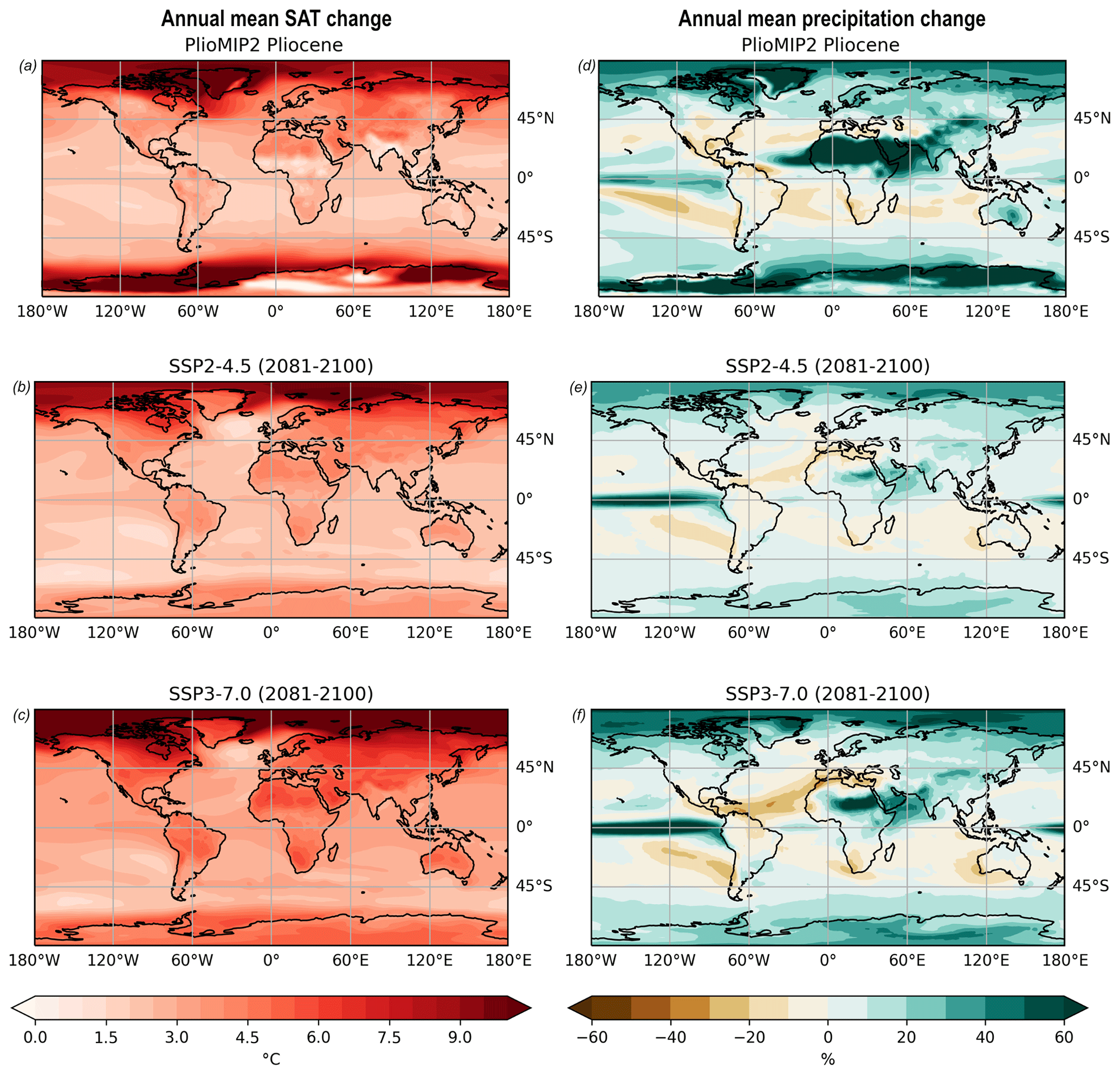
Figure 1 PlioMIP2 ensemble MIS KM5c SAT (a) and precipitation (d) anomalies relative to the PI compared to equivalent CMIP6 anomalies for 2081–2100 under SSP2-4.5 (b, e) and SSP3-7.0 (c, f). The PlioMIP2 ensemble includes all 16 models in Haywood et al. (2020) plus HadGEM3 (Williams et al., 2021). The CMIP6 data are from the IPCC WGI Interactive Atlas (Gutiérrez et al., 2021). CMIP6 SAT anomalies (b, c) are relative to 1850–1900, and precipitation anomalies (e, f) are relative to the standard CMIP6 base period (1995–2014). Note that the models included in PlioMIP2 are not all included in CMIP6.

From the water cycle projections in the IPCC AR6 (Table 8.1 in Douville et al., 2021), it is clear that the global mean percentage change in precipitation is also comparable between 2081–2100 under SSP2-4.5 (4.0 %) and under SSP3-7.0 (5.1 %) relative to the CMIP6 base period (1995–2014) and the Pliocene (7 %; Haywood et al., 2020). Similar spatial features include the wetting of the Sahara and polar regions and the drying of the Caribbean, off the western coast of South America (Fig. 1d–f).

However, caution must be applied when referencing the Pliocene as a palaeoclimate analogue given the importance of – continually changing – anthropogenic greenhouse gas forcing in present day.

Here, we begin to assess the role of CO₂ forcing in the Pliocene compared to other drivers of climate and changes in boundary conditions. The non-CO₂ forcing we refer to includes changes to ice sheets and “orography”, the latter of which also includes changes to prescribed vegetation, bathymetry, land–sea mask, soils, and lakes, as per the experimental design of PlioMIP2 (Haywood et al., 2016).

1.2 Drivers of Pliocene climate

Though there are similarities in large-scale climate features between the Pliocene and end-of-century projections in AR6, the similarity in the causes and drivers of some of these features is yet to be fully assessed.

Previous studies on the drivers of Pliocene temperature change have used energy balance analyses. These are commonly applied in palaeoclimate studies to understand changes in temperature by separating out individual forcing components (e.g. Lunt et al., 2012; Hill et al., 2014, and references therein).

Lunt et al. (2012) combined a novel factorisation methodology with energy balance analysis to assess the causes of Pliocene warmth in HadCM3 using the PRISM2 boundary conditions (Dowsett et al., 1999). CO₂ was found to cause 36 %–61 % of Pliocene warmth, orography was found to cause 0 %–26 %, ice sheets were found to cause 9 %–13 %, and vegetation was found to cause 21 %–27 %. These drivers were found to have spatial variation in importance, with changes in orography and ice sheets being particularly important in driving polar amplification in the northern high latitudes and orography being particularly important in the southern high latitudes. The energy balance analysis also highlighted how surface albedo changes and direct CO₂ forcing contributed more than cloud feedbacks, with surface albedo changes dominating at middle and high latitudes and CO₂ forcing dominating at low latitudes.

Hill et al. (2014) developed the methodology of Lunt et al. (2012) and conducted the first multi-model energy balance analysis using the eight models included in PlioMIP1 Experiment 2, forced with the PRISM3 boundary conditions (Dowsett et al., 2010). Greenhouse gas emissivity was found to be the dominant cause of warming in the tropics. There were large uncertainties between models in the high latitudes, but all energy balance components were important, and clear-sky albedo was the dominant driver of polar amplification through reductions in ice sheets, sea ice, and snow cover and through changes to vegetation. The relative influence of the energy balance components was more uncertain in the northern mid-latitudes, particularly in the North Atlantic and Kuroshio Current regions, where warming was also simulated differently between models (Haywood et al., 2013).

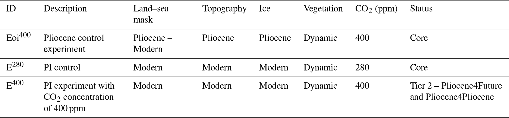
Developing from PlioMIP1, forcing factorisation experiments were included in PlioMIP2 to enable the explicit assessment of forcing components (Haywood et al., 2016). These experiments included Pliocene simulations with PI ice configuration (experiment Eo⁴⁰⁰) and PI orography configuration (experiment Ei⁴⁰⁰), as well as a PI simulation with Pliocene-level CO₂ concentration (experiment E⁴⁰⁰); the PlioMIP2 experimental design and naming conventions were shown in Haywood et al. (2016). These forcing factorisation experiments were in Tier 2 of the experimental design, meaning they were optional and completed by a smaller number of model groups.

The impact of various mechanisms on Pliocene climate has been studied using energy balance analysis in individual PlioMIP2 models. Using the PlioMIP2 forcing factorisation experiments and methodology proposed in Haywood et al. (2016), Chandan and Peltier (2018) assessed the mechanisms of Pliocene climate in the CCSM4-UoT model. They found that around 1.67 ^∘C (45 %) of warming was attributable to CO₂ forcing, 1.54 ^∘C (42 %) of warming was attributable to changes in orography, and 0.47 ^∘C (13 %) of warming was attributable to a reduction in ice sheets. Using the same factorisation methodology for the COSMOS model, Stepanek et al. (2020) found that 2.23 ^∘C (∼66 %) of warming was attributable to CO₂ forcing, 0.91 ^∘C (∼25 %) of warming was attributable to orography, and 0.38 ^∘C (∼13 %) of warming was attributable to changes in the ice sheets.

An updated methodology of Lunt et al. (2012) and Hill et al. (2014) is used to explore drivers of northern high-latitude warmth in the CCSM4 model in Feng et al. (2017). Changes to regional topography, Arctic sea ice and the Greenland ice sheet, and the North Atlantic Meridional Overturning Circulation were found to explain the amplification of SAT in the northern high latitudes. Greenhouse gas emissivity was also found to be important, particularly with the subsequent positive feedbacks which have a more distributed effect. This updated methodology is also used in Feng et al. (2019), where it is demonstrated that a seasonally sea-ice-free Pliocene Arctic Ocean can be simulated in CESM1.2 by including aerosol–cloud interactions and by excluding industrial pollutants.

To date, there has been no systematic study comparing multiple models in the PlioMIP2 ensemble to spatially quantify the importance of different climate forcings, nor have climate variables other than SAT been previously assessed in multiple models in a single study. Here, we present the relative spatial influence of CO₂ forcing on SAT across multiple PlioMIP2 models and, for the first time, on sea surface temperature (SST) and precipitation. We employ the forcing factorisation experiments of PlioMIP2 and a novel, simple linear factorisation method with outputs we term “FCO₂”.

2 Methods

2.1 Model boundary conditions

Standardised boundary conditions are used by all model groups for the core Pliocene control experiment in PlioMIP2, derived from the US Geological Survey PRISM4 reconstruction (Dowsett et al., 2016) and implemented as described in Haywood et al. (2016). These boundary conditions include spatially complete gridded datasets at $\mathrm{1}{}^{\circ }\times \mathrm{1}{}^{\circ }$ of latitude–longitude for land–sea distribution, topography and bathymetry, vegetation, soil, lakes, and land ice cover; all models analysed here use the enhanced version of the boundary conditions, meaning they include all reconstructed changes to the land–sea mask and ocean bathymetry (Haywood et al., 2020).

The configuration of the Greenland ice sheet in PRISM4 is based upon the results from the Pliocene Ice Sheet Modelling Intercomparison Project (PLISMIP); it is confined to high elevations in the eastern Greenland mountains and covers an area of around 25 % of the modern ice sheet (Dolan et al., 2015; Koenig et al., 2015). Ice coverage over Antarctica has been debated (see Levy et al., 2022), but the PRISM3 Antarctic ice configuration – in which there is a reduction in the ice margins in the Wilkes and Aurora basins in eastern Antarctica, while western Antarctica is largely ice free (Dowsett et al., 2010) – is supported and so retained in the PRISM4 reconstruction (Dowsett et al., 2016). Later modelling studies further support the potential for ice retreat in similar areas in Antarctica under the warmer temperatures of the Pliocene (e.g. DeConto and Pollard, 2016).

The palaeogeography is broadly similar to modern except for the closure of the Bering Strait and the Canadian Arctic Archipelago; the changes in the Torres Strait, Java Sea, South China Sea, and Kara Strait; and the presence of a western Antarctic seaway (Haywood et al., 2016). PRISM4 also includes, for the first time, dynamic topography and glacial isostatic adjustment to inform the representation of local sea level (Dowsett et al., 2016).

The atmospheric CO₂ concentration is set to 400 ppm, and in the absence of proxy data, all other trace gases are set to be identical to the concentrations in the PI control experiment for each individual model group (Haywood et al., 2016).

2.2 Participating models

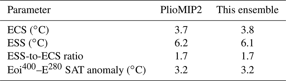
A total of 7 of the 17 models of the PlioMIP2 ensemble are included in this study, as they conducted the necessary experiments for an application of our novel FCO₂ method, namely Eoi⁴⁰⁰, E⁴⁰⁰, and E²⁸⁰ (see Sect. 2.3). This subgroup is also found to be representative of the wider PlioMIP2 ensemble in terms of modelled ECS, ESS, and global mean Eoi⁴⁰⁰–E²⁸⁰ SAT anomaly (Table 1).

Table 1 A comparison of climate parameters between the PlioMIP2 ensemble and the subgroup of PlioMIP2 models used here.

The models are of varying ages and resolutions. Summaries of details relevant to PlioMIP2 are shown in Haywood et al. (2020) and in individual model papers for the PlioMIP2 experiments, which are cited in Table 2.

Table 2 Details of the climate models used in the FCO₂ analysis (adapted from Haywood et al., 2020).

Table 3 Details of the PlioMIP2 experiments included in the FCO₂ analysis (adapted from Haywood et al., 2016). Note that dynamic vegetation was optional in the experimental design; only COSMOS ran with dynamic vegetation, and all other models ran with the prescribed vegetation of Salzmann et al. (2008). As COSMOS ran with dynamic vegetation, some vegetation feedback in this model will be included in the E⁴⁰⁰-E²⁸⁰ anomaly.

2.3 FCO₂ method

Taking advantage of the forcing factorisation experiments included in the PlioMIP2 experimental design, here we propose a novel, simple linear factorisation method to assess the influence of CO₂ forcing with outputs we term FCO₂. We apply the FCO₂ method to all seven models for SAT and precipitation and to six models for SST; IPSLCM5A2 is excluded for analysis of the latter, as only 10 model years of data were available.

The method uses three PlioMIP2 experiments: the two core experiments (E²⁸⁰ and Eoi⁴⁰⁰) and one Tier 2 experiment (E⁴⁰⁰; Table 3). Core experiments were completed by all PlioMIP2 modelling groups, and Tier 2 experiments were submitted by a smaller number of modelling groups. The seven models included here were the only ones to have reported E⁴⁰⁰ results by the time of compiling this study.

We define FCO₂ as an approximation of the relative influence of CO₂, calculated by the following:

$$\begin{array}{}\text{(1)}& {\mathrm{FCO}}_{\mathrm{2}}={\displaystyle \frac{({\text{E}}^{\mathrm{400}}-{\text{E}}^{\mathrm{280}})}{({\text{Eoi}}^{\mathrm{400}}-{\text{E}}^{\mathrm{280}})}},\end{array}$$

where E⁴⁰⁰–E²⁸⁰ represents the change in climate caused by the change in CO₂ concentration from 280 to 400 ppm alone, and Eoi⁴⁰⁰–E²⁸⁰ represents the change in climate as a result of implementing the full Pliocene boundary conditions.

FCO₂ is therefore a fractional quantity where a value of 1.0 denotes that the signal of change is wholly dominated by CO₂ forcing, and a value of 0.0 denotes the contrasting case where the climate signal is wholly dominated by non-CO₂ forcing. Here, non-CO₂ forcing is defined as changes to ice sheets and orography, the latter of which includes changes to prescribed vegetation, bathymetry, land–sea mask, soils, and lakes, as per the PlioMIP2 experimental design (Haywood et al., 2016). Our full interpretation of the range of FCO₂ values is shown in Table 4.

Table 4 Interpretation of FCO₂ values.

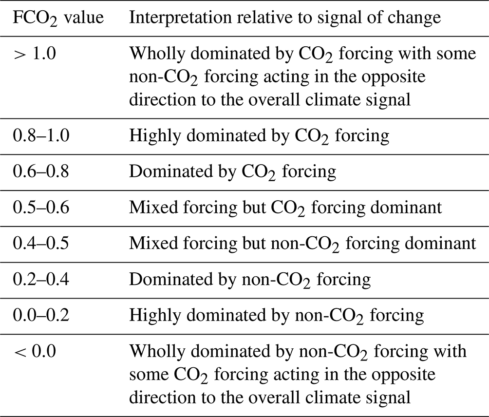
FCO₂ values are not limited to values between 0.0 and 1.0. FCO₂ values above 1.0 represent a climate that is wholly dominated by CO₂ forcing, where non-CO₂ forcing creates an opposing climatic effect. Similarly, FCO₂ values below 0.0 represent a climate that is wholly dominated by non-CO₂ forcing, where CO₂ forcing creates an opposing climatic effect.

This becomes clear if one considers FCO₂ in the case of SAT and SST. The Pliocene climate is characterised as having elevated temperature and CO₂ concentration compared to the PI (e.g. Dowsett et al., 2016; Haywood et al., 2020); so, given that the predominant effect of CO₂ forcing is warming, an FCO₂ value below 0.0 is rare. An exception is provided by higher-order effects where CO₂ leads to a cooling (see Sherwood et al., 2020). FCO₂ values below 0.0 for SAT are limited to central Antarctica, where the overall Pliocene climate change is a cooling with respect to the PI (see Sect. 3.2), and there are no FCO₂ values below 0.0 for SST.

We consider uncertainty in the FCO₂ method in terms of whether there is consistent agreement between the individual models on whether CO₂ forcing or non-CO₂ forcing is the most important driver (i.e. whether FCO₂>0.5 or FCO₂<0.5). In this paper, we deem FCO₂ to be uncertain if four or fewer models agree on the dominant forcing (see Fig. 7, Sect. 4.1).

In checking for non-linearity, we consider an additional PlioMIP2 simulation that tests the effect of Pliocene boundary conditions with PI-level CO₂ concentration (Eoi²⁸⁰). The sum contributions of CO₂ and non-CO₂ factors relative to the total Eoi⁴⁰⁰–E²⁸⁰ anomaly is close to zero (Eq. 2; Fig. S1 in the Supplement), meaning that any factors not considered in these experiments – i.e. anything other than CO₂ concentration, changes to ice sheets, orography, and/or vegetation – are unlikely to be a dominant cause of change. Non-linearity is tested for in the four models which had reported Eoi²⁸⁰ results by the time of compiling this study, namely CCSM4-UoT, COSMOS, HadCM3, and MIROC4m. Additional checks with the other models would likely further confirm the linearity, highlighting the utility in more modelling groups completing the forcing factorisation experiments in PlioMIP2 and future phases.

$$\begin{array}{}\text{(2)}& ({\text{Eoi}}^{\mathrm{400}}-{\text{E}}^{\mathrm{280}})-\left[\right({\text{E}}^{\mathrm{400}}-{\text{E}}^{\mathrm{280}})+({\text{Eoi}}^{\mathrm{280}}-{\text{E}}^{\mathrm{280}}\left)\right]\approx \mathrm{0}\end{array}$$

2.4 Energy balance analysis

Results from the FCO₂ method are compared to an energy balance analysis using the methodology of Hill et al. (2014). This methodology was developed from the factorisation methodology of Heinemann et al. (2009) and Lunt et al. (2012) and assumed that the change in SAT was largely driven by CO₂, orography, ice sheets, and vegetation and that any other changes (such as soils or lakes) had a negligible impact.

$$\begin{array}{}\text{(3)}& \mathrm{\Delta }T=\mathrm{d}{T}_{{\mathrm{CO}}_{\mathrm{2}}}+\mathrm{d}{T}_{\text{orog}}+\mathrm{d}{T}_{\text{ice}}+\mathrm{d}{T}_{\text{veg}}\end{array}$$

In the Hill et al. (2014) methodology, the temperature at each latitude in a GCM experiment is given by the following:

$$\begin{array}{}\text{(4)}& T={\left({\displaystyle \frac{{\text{SW}}_{\text{TOA}}^{\downarrow }(\mathrm{1}-\mathit{\alpha })-H}{\mathit{\epsilon }\mathit{\sigma }}}\right)}^{\mathrm{1}/\mathrm{4}}\equiv T(\mathit{\epsilon },\mathit{\alpha },H),\end{array}$$

with the temperature anomaly approximated by a linear combination of contributions from changes in emissivity (ΔT_ε), albedo (ΔT_α), and heat transport (ΔT_H). Temperature changes due to emissivity and albedo can be further separated to include changes attributed to the impact of atmospheric greenhouse gases (ΔT_ggε), clouds (through impacts on emissivity, ΔT_cε, and albedo, ΔT_cα), and clear-sky albedo (ΔT_csα). The effect of changes in temperature due to topography (ΔT_topo) is also important to consider when comparing the Pliocene to the PI, where specific details differ (Dowsett et al., 2016).

$$\begin{array}{}\text{(5)}& \mathrm{\Delta }T\approx \mathrm{\Delta }{T}_{\text{gg}\mathit{\epsilon }}+\mathrm{\Delta }{T}_{\mathrm{c}\mathit{\epsilon }}+\mathrm{\Delta }{T}_{\mathrm{c}\mathit{\alpha }}+\mathrm{\Delta }{T}_{\text{cs}\mathit{\alpha }}+\mathrm{\Delta }{T}_{\mathrm{H}}+\mathrm{\Delta }{T}_{\text{topo}},\end{array}$$

where

$$\begin{array}{}\text{(6)}& \mathrm{\Delta }{T}_{\text{gg}\mathit{\epsilon }}=T({\mathit{\epsilon }}_{\text{cs}},\mathit{\alpha },H)-T({\mathit{\epsilon }}_{\text{cs}}^{\prime },\mathit{\alpha },H)-\mathrm{\Delta }{T}_{\text{topo}},\end{array}$$

and

$$\begin{array}{}\text{(7)}& \mathrm{\Delta }{T}_{\text{topo}}=\mathrm{\Delta }h\cdot \mathit{\gamma },\end{array}$$

in which Δh is the change in topography (Pliocene–PI), and γ is a constant atmospheric lapse rate (≈5.5 K km⁻¹; Yang and Smith, 1985; Hill et al., 2014).

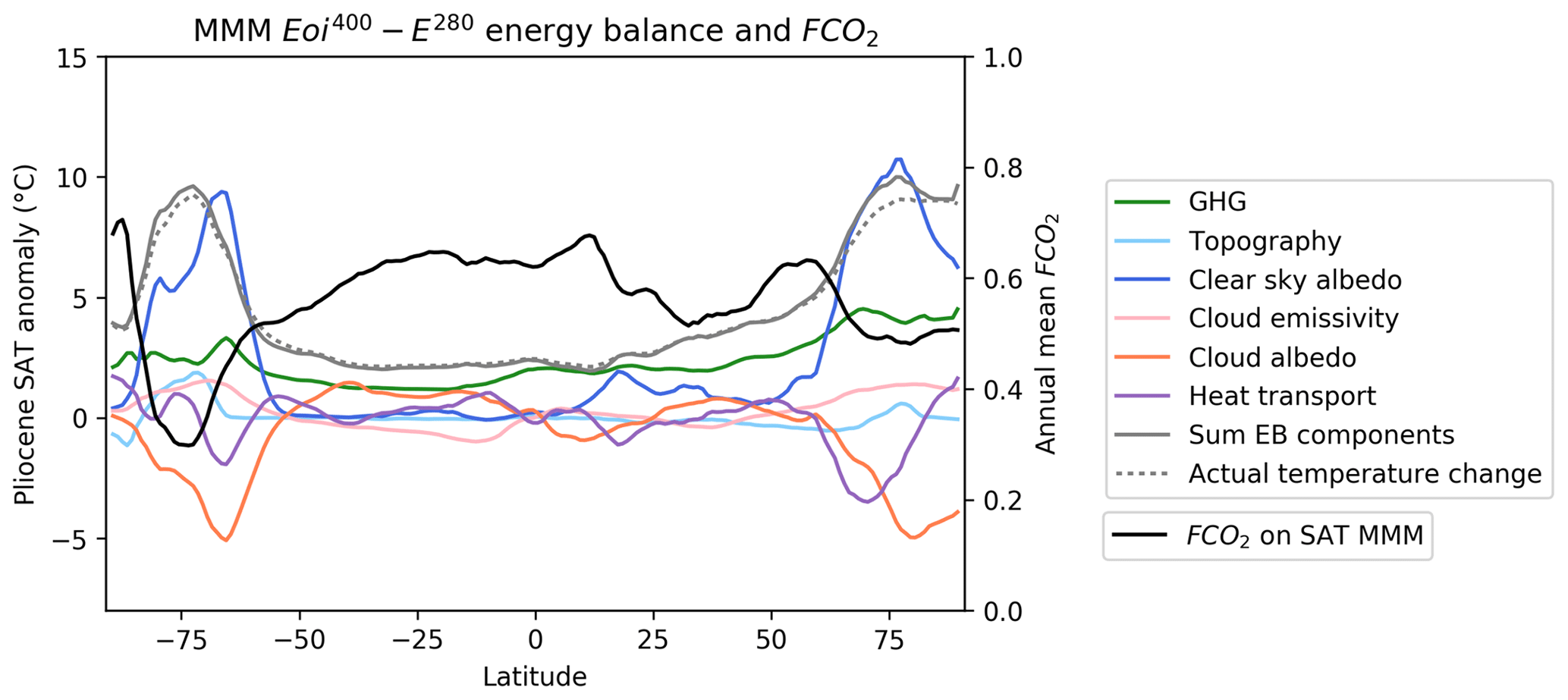
Figure 2 The MMM Eoi⁴⁰⁰–E²⁸⁰ energy balance with the FCO₂ of the SAT MMM. The MMM includes HadCM3, COSMOS, CCSM4-UoT, CESM2, MIROC4m, and NorESM1-F for both the energy balance and FCO₂ (IPSLCM5A2 is excluded because the required fields were not available for the energy balance analysis). The degree of Pliocene warming attributable to each energy balance component at each degree of latitude is shown, and the sum of the energy balance terms (solid grey line) agrees well with the simulated temperature change (dashed grey line). The FCO₂ of the SAT at 0.70 MMM is shown in the solid black line with a separate axis to compare to the energy balance.

This more approximate methodology is chosen over the further-modified methodology of Feng et al. (2017) – in which an amended approximate partial radiative perturbation method was applied to calculate cloudy-sky albedo more accurately in polar regions, and zonal heat transport was separated into atmosphere and ocean components – as it was used to assess the PlioMIP1 ensemble and thus provides directly comparable outputs.

Six of the seven models for which FCO₂ is quantified are considered in the energy balance analysis; IPSLCM5A2 is excluded because the required fields were not available for this model. Model-specific topography files are used as they were implemented in the individual model E²⁸⁰ and Eoi⁴⁰⁰ experiments to minimise uncertainties that may arise due to different implementation methods, and the energy balance components are compared to the simulated temperature change and outputs of the FCO₂ method. The multi-model mean (MMM) energy balance is calculated using the MMM of each of the individual components as follows:

$$\begin{array}{}\text{(8)}& \stackrel{\mathrm{‾}}{\mathrm{\Delta }T}\approx \stackrel{\mathrm{‾}}{\mathrm{\Delta }{T}_{\text{gg}\mathit{\epsilon }}}+\stackrel{\mathrm{‾}}{\mathrm{\Delta }{T}_{\mathrm{c}\mathit{\epsilon }}}+\stackrel{\mathrm{‾}}{\mathrm{\Delta }{T}_{\mathrm{c}\mathit{\alpha }}}+\stackrel{\mathrm{‾}}{\mathrm{\Delta }{T}_{\text{cs}\mathit{\alpha }}}+\stackrel{\mathrm{‾}}{\mathrm{\Delta }{T}_{\mathrm{H}}}+\stackrel{\mathrm{‾}}{\mathrm{\Delta }{T}_{\text{topo}}}.\end{array}$$

Comparing the SAT outputs of the energy balance analysis with outputs of the FCO₂ method on SAT allows the accuracy of our novel method to be assessed and also aids in the interpretation of, and adds nuance to, the FCO₂ results. In order to assess the accuracy of the simple linear estimate and to further validate the FCO₂ method, we compare ΔT_ggε to the E⁴⁰⁰–E²⁸⁰ SAT anomaly, and we compare the sum of ΔT_cε, ΔT_cα, ΔT_csα, ΔT_H, and ΔT_topo to the Eoi⁴⁰⁰–E⁴⁰⁰ SAT anomaly.

3 Results

3.1 Energy balance analysis

The Eoi⁴⁰⁰–E²⁸⁰ energy balance analysis unravels the relative contributions of CO₂, topography, cloud emissivity, clear-sky albedo, and heat transport to the Eoi⁴⁰⁰–E²⁸⁰ SAT anomaly (Fig. 2). The energy balance analysis for the sub-group of PlioMIP2 models presented here supports the findings of the PlioMIP1 ensemble presented in Hill et al. (2014): clear-sky albedo is the dominant driver of warming and polar amplification in the high latitudes, and greenhouse gas emissivity is the dominant driver in the low latitudes. The zonal influence of CO₂ on Pliocene warming also appears relatively consistent across latitudes, as in Hill et al. (2014); there is some amplification at high latitudes, particularly in the Northern Hemisphere, but this amplification is smaller than that seen for other energy balance components.

The FCO₂ method provides an alternative estimate for the relative contribution of CO₂ to changes in SAT compared to the energy balance analysis. FCO₂ is lower than the greenhouse gas contribution as computed in the energy balance analysis at the high latitudes (with the exception of the very high latitudes in the Southern Hemisphere) where there is a greater contribution from clear-sky albedo and topography. Conversely, it is higher in the middle and low latitudes where CO₂ is the dominant energy balance component.

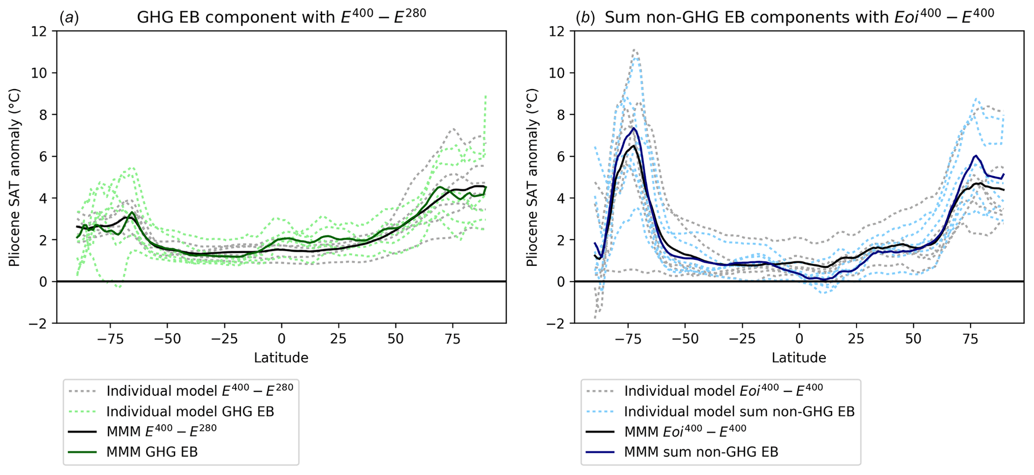
Figure 3 Comparison of the greenhouse gas (GHG) energy balance component (ΔT_ggε) and the E⁴⁰⁰–E²⁸⁰ SAT anomaly (a) and equivalent comparison of the sum of non-greenhouse gas energy balance components and the Eoi⁴⁰⁰–E⁴⁰⁰ anomaly (b). The MMM is shown in a solid line, and individual models are shown by dotted lines, representing uncertainty between models.

The energy balance analysis provides more nuance with regard to the specific drivers of change than the FCO₂ method, which only indicates whether warming is due to CO₂ forcing or non-CO₂ forcing. Using the energy balance analysis in tandem with FCO₂, we are able to understand which component(s) within the encompassing non-CO₂ category is (are) most influential. For example, the energy balance analysis highlights how clear-sky albedo has the largest influence on Pliocene warming in the high latitudes, whereas the FCO₂ method suggests that non-CO₂ factors are important. Furthermore, the energy balance analysis helps to explain the reasons for FCO₂ values above 1 for SAT; for example, although only at a zonal scale, the energy balance analysis shows that topography acts to lower SAT at the South Pole. However, the FCO₂ method provides spatial nuance not possible with the energy balance analysis (see Sect. 4.1).

The energy balance analysis can also be compared with the E⁴⁰⁰–E²⁸⁰ and Eoi⁴⁰⁰–E⁴⁰⁰ SAT anomalies (Fig. 3). The greenhouse gas energy balance component (ΔT_ggε) is seen to be in good agreement with the E⁴⁰⁰–E²⁸⁰ SAT anomaly (Fig. 3a), with global mean increases in SAT of 1.97 and 1.85 ^∘C, respectively. The energy balance component shows more variability and uncertainty between models than the E⁴⁰⁰–E²⁸⁰ anomaly, and it also shows more zonal variation.

The sum of the non-greenhouse-gas energy balance components is also seen to be in good agreement with the Eoi⁴⁰⁰–E⁴⁰⁰ anomaly (Fig. 3b), with global mean increases in SAT of 1.38 and 1.49 ^∘C, respectively. There is more uncertainty between models for the Eoi⁴⁰⁰–E⁴⁰⁰ anomaly, highlighting the different implementations of ice sheets and land–sea masks in the Eoi⁴⁰⁰ experiment.

That the absolute anomalies and energy balance components agree provides an additional argument for the accuracy and usefulness of the simple linear estimations used in the FCO₂ method and hence enables the first estimates of the drivers of SST (Sect. 3.3) and precipitation (Sect. 3.4), as well as more spatially detailed estimates of the drivers of SAT (Sect. 3.2).

3.2 Surface air temperature

The MMM Eoi⁴⁰⁰–E²⁸⁰ global mean SAT anomaly is 3.2 ^∘C, equal to the anomaly of the PlioMIP2 ensemble (Haywood et al., 2020). The range is also equal to that of the PlioMIP2 ensemble, with end members NorESM1-F and CESM2 simulating the smallest (1.7 ^∘C) and largest (5.2 ^∘C) Eoi⁴⁰⁰–E²⁸⁰ anomalies, respectively (Haywood et al., 2020). Warming occurs in all regions and is amplified in the high latitudes, except for an isolated region of cooling in central Antarctica (Fig. 4a).

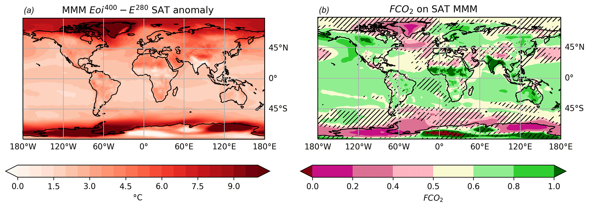
Figure 4 MMM Eoi⁴⁰⁰ minus E²⁸⁰ SAT anomaly (a) and FCO₂ of the MMM for SAT (b). The hatching in (b) represents where there is no consistent agreement between models on whether CO₂ forcing or non-CO₂ forcing is the most important (i.e. whether FCO₂>0.5 or FCO₂<0.5).

The MMM global mean FCO₂ is 0.56 (individual model range 0.40–0.70; Fig. S2), meaning 56 % of the SAT change is due to CO₂ forcing. FCO₂ varies around the globe (Fig. 4b); CO₂ is the most important forcing in large areas of the low latitudes and, predictably, becomes less important in the high latitudes due to the significant changes in ice sheets and orography in the Pliocene. FCO₂ is found to be similar over land and ocean, with mean values of 0.58 and 0.56, respectively.

Many areas of highly dominant CO₂ forcing (FCO₂ 0.8–1.0) are found on land, specifically over central Africa, the Indian subcontinent, and parts of Australia, Antarctica, and North America. Parts of these areas have FCO₂ values above 1.0, indicating that non-CO₂ forcing acts in the opposite direction to the overall signal. However, high FCO₂ is also seen in the Pacific Ocean off the western coast of North America and in the Barents Sea south of Svalbard.

There is a small region in the North Atlantic off the eastern coast of North America where non-CO₂ forcing is dominant (FCO₂ 0.2–0.4), but regions where non-CO₂ forcing is highly dominant (FCO₂ 0.0–0.2) are mostly limited to Antarctica and Greenland, evidencing the role of changes to orography and ice sheets in polar amplification in the Pliocene. In central Antarctica, there is also a region where FCO₂ is below 0.0, indicating that CO₂ forcing acts to warm the climate against an overall signal of cooling.

The FCO₂ method shows CO₂ to be the most important forcing overall, but there is also a significant contribution from non-CO₂ forcing which should not be overlooked, particularly if we are to learn from the Pliocene as an analogue for the future. Regions of uncertainty are generally found where the dominant forcing is mixed (FCO₂ 0.4–0.6), but there is also uncertainty in some regions of dominant and highly dominant CO₂ forcing (FCO₂ 0.6–1.0), including central and eastern Antarctica, the Barents Sea, and isolated regions of central Africa and of the Indian subcontinent (Fig. 4b). Other notable regions of uncertainty include the North Atlantic and northwest Pacific, consistent with the findings of Hill et al. (2014); however, in our analysis of PlioMIP2 simulations, we find that the northern mid-latitudes appear to have more certainty than in the PlioMIP1 ensemble.

3.3 Sea surface temperature

The MMM Eoi⁴⁰⁰–E²⁸⁰ global mean SST anomaly is 2.3 ^∘C, which is again equal to the global mean anomaly of the PlioMIP2 ensemble. The anomaly also sits relatively centrally in relation to the PlioMIP2 ensemble range of 1.3–3.9 ^∘C (Haywood et al., 2020). Warming is seen in all ocean basins, with amplification in the high latitudes, particularly in the Labrador Sea and the North Atlantic (Fig. 5a).

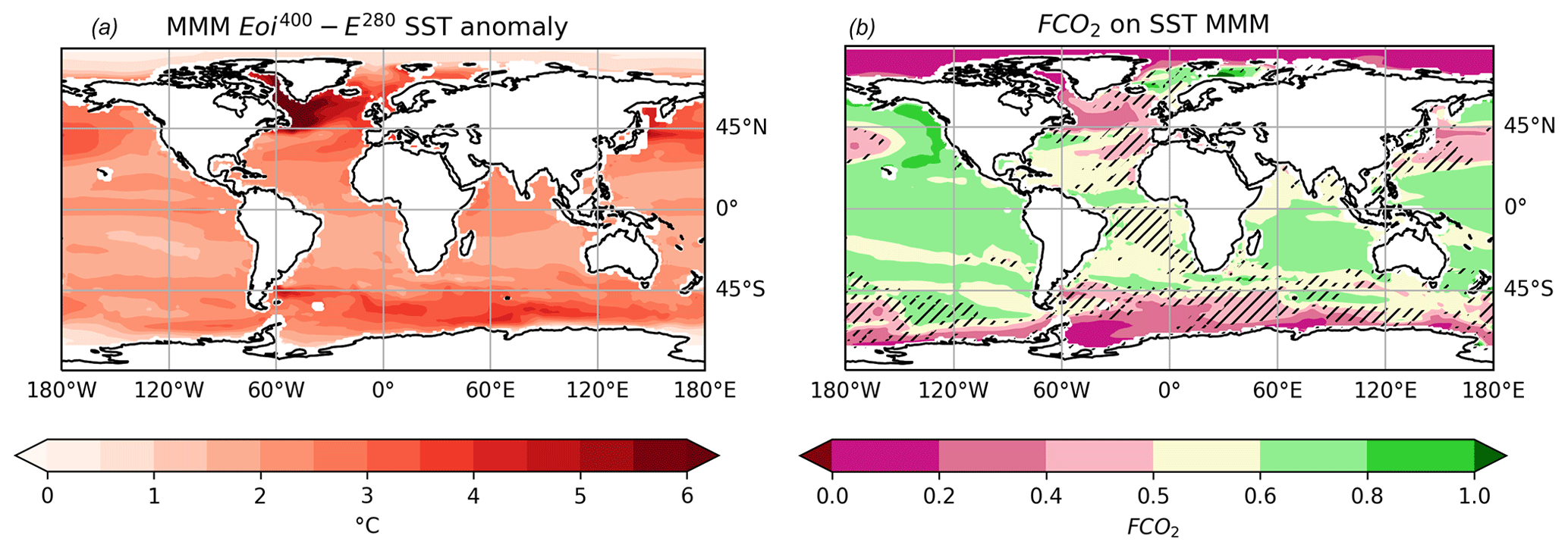
Figure 5 MMM Eoi⁴⁰⁰ minus E²⁸⁰ SST anomaly (a) and FCO₂ of the MMM for SST (b). IPSLCM5A2 is excluded from SST analysis due to limited data availability. The hatching in (b) represents where there is no consistent agreement between models on whether CO₂ forcing or non-CO₂ forcing is the most important (i.e. whether FCO₂>0.5 or FCO₂<0.5).

The MMM global mean FCO₂ is 0.56 (individual model range 0.40–0.76; Fig. S3), meaning 56 % of the SST change is due to CO₂ forcing. The MMM global mean FCO₂ on SST is the same as the MMM global mean FCO₂ on SAT, and there are comparable spatial features at low and mid-latitudes. On the other hand, FCO₂ on SST is significantly lower than on SAT at high latitudes (Fig. 5b), indicating that changes in orography and ice sheets, and feedbacks including sea ice, have a much larger influence on SST than on SAT.

Non-CO₂ forcing is dominant or highly dominant (FCO₂ 0.0–0.4) in the Arctic Sea, and it is dominant in much of the Southern Ocean. SST in the South Atlantic is also more strongly driven by non-CO₂ forcing compared to SAT in the region, perhaps indicating a change in ocean circulation driven by these non-CO₂ forcings consistent with previous work (e.g. Hill et al., 2017). No regions of FCO₂ below 0.0 are seen.

The amplified warming seen in the Labrador Sea and the North Atlantic appears to be predominantly driven by non-CO₂ forcing (FCO₂ 0.2–0.4), but the warming pattern also extends to regions where forcing is mixed (FCO₂ 0.4–0.6) or, south of Svalbard, where forcing is even dominated by CO₂ (FCO₂ 0.6–0.8).

Regions of uncertainty in FCO₂ on SST largely mirror those for SAT over the sea surface and are predominantly found in regions of mixed forcing (FCO₂ 0.4–0.6) and in the middle and southern high latitudes. Unlike for SAT, SSTs in the Arctic Ocean show good agreement that non-CO₂ forcing is highly dominant (FCO₂ 0.0–0.2). This difference in consistency between FCO₂ on SAT and FCO₂ on SST might relate to the different distributions of sea ice between models.

3.4 Precipitation

The MMM Eoi⁴⁰⁰–E²⁸⁰ precipitation anomaly is 0.18 mm d⁻¹ or 6.4 % compared to the PlioMIP2 ensemble value of 7 % (range 2 %–13 %; Haywood et al., 2020).

Particularly large increases in precipitation are seen in northern Africa and in the Middle East, as well as over Greenland and parts of Antarctica (Fig. 6a). The MMM spatial pattern of precipitation change is more complex than that seen for SAT and SST but is representative of the whole PlioMIP2 ensemble (Figs. 6a and 1d).

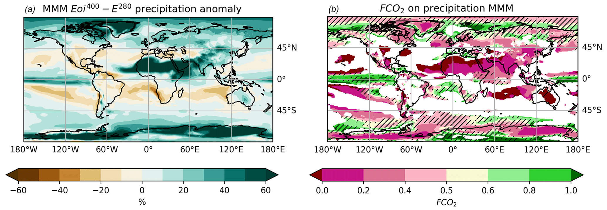
Figure 6 MMM Eoi⁴⁰⁰ minus E²⁸⁰ precipitation anomaly (a) and FCO₂ of MMM for precipitation (b). In (b), regions of Eoi⁴⁰⁰–E²⁸⁰ precipitation change of less than 10 % are masked (white), and hatching represents where there is no consistent agreement between models on whether CO₂ forcing or non-CO₂ forcing is the most important (i.e. whether FCO₂>0.5 or FCO₂<0.5).

The spatial pattern of FCO₂ on precipitation is also more complex than that seen for SAT and SST; areas with a percentage change of less than 10 % are masked in white to increase clarity and to reduce noise (Fig. 6b). The MMM global mean FCO₂ is 0.51 (individual model range 0.39–0.69; Fig. S4), meaning CO₂ forcing causes 51 % of the change in global mean precipitation, and so non-CO₂ forcing plays a slightly more important role in changes in precipitation than is the case for SAT and SST. For precipitation, there is a large difference in FCO₂ over land compared to oceans, with mean values of 0.23 and 0.58, respectively; non-CO₂ forcing is much more important over land.

The largest increases in precipitation are generally driven by non-CO₂ forcing, seen over northern Africa and the Indian subcontinent (see Feng et al., 2022), Greenland, and parts of eastern and western Antarctica. Parts of northern Africa have FCO₂ values below 0.0, indicating that CO₂ is acting to limit this increase in precipitation. FCO₂ values below 0.0 are also seen in central Australia, central North America, and parts of the tropical Indian, Atlantic, and Pacific oceans, where the signals in precipitation anomaly are both positive and negative.

Non-CO₂ forcing is also dominant (FCO₂ 0.2–0.4) or highly dominant (FCO₂ 0.0–0.2) in some regions of precipitation decrease, including the tropical South Pacific, and in the regions west of the maritime continent and off the eastern coast of North America.

There are also regions where FCO₂ is above 1.0 in parts of central and eastern Antarctica, the tropical Pacific, the Barents Sea, and a small area in both the Bering Sea and the Arctic Ocean north of Alaska. These are mostly regions of small precipitation increase, indicating that non-CO₂ forcing acts to decrease precipitation despite the overall increase.

Spatial changes appear to be predominantly driven by non-CO₂ forcing, whereas CO₂ forcing has a more muted and widespread effect. The overall effect of CO₂ is an increase in global mean precipitation, although we see both increases and decreases in precipitation regionally, which appear to be attributable to non-CO₂ forcing such as changes in orography, ice sheets, and/or vegetation. That such local changes have a notable effect on the Pliocene precipitation anomaly may limit the degree to which we can use the Pliocene as a precipitation analogue for our warmer future.

There is more uncertainty between models for FCO₂ on precipitation than for SAT and SST. Uncertainty is seen in regions of both mixed forcing (FCO₂ 0.4–0.6) and of dominant or highly dominant CO₂ forcing (FCO₂ 0.6–1.0). Regions predominantly driven by non-CO₂ forcing (FCO₂ 0.0–0.4) show better agreement between models, suggesting that the impact of non-CO₂ forcing is more robustly represented in the PlioMIP2 ensemble than the impact of CO₂ on precipitation.

4 Discussion

4.1 FCO₂ method

The FCO₂ method has been validated by comparing outputs to the energy balance analysis, and it presents a great opportunity to expand our understanding of climate drivers in the Pliocene and beyond.

We devised a novel method to quantitatively estimate the drivers of Pliocene SST and precipitation. This method can be applied to other climate variables with relative ease and little computational cost and also to other ensembles of models beyond PlioMIP2.

Aided by comparison to the energy balance analysis, the FCO₂ method provides a complete view of drivers of Pliocene climate at both global and regional scales; in particular, the contributions of CO₂ vs. non-CO₂ forcing to SAT, SST, and precipitation on local and regional scales are revealed. We also show how comparison to the energy balance analysis adds insight into feedbacks and other such indirect effects of CO₂ forcing which the FCO₂ method does not capture.

This work has also highlighted the value and accuracy of using the E⁴⁰⁰–E²⁸⁰ and Eoi⁴⁰⁰–E⁴⁰⁰ SAT anomalies as estimates for ΔT_ggε and the sum of the non-greenhouse gas components in energy balance analyses, respectively. This shows that, while exact information on the drivers of temperature still depend on the application of a more elaborated and computationally expensive set of sensitivity simulations, a good degree of knowledge may be derived by applying a much smaller number of simulations. Not only is this more economic, but it may also increase the number of modelling groups that take part in future model intercomparison studies of the kind that we have presented here. The FCO₂ method, requiring a smaller number of simulations compared to the energy balance analyses, has allowed for a larger ensemble of models to be assessed than previously possible in PlioMIP2.

The FCO₂ method also allows for an assessment of the uncertainty between models with regard to the drivers of the different climate variables by comparing where there is (not) consistent agreement on the forcing, i.e. whether FCO₂>0.5 or FCO₂<0.5 (Fig. 7).

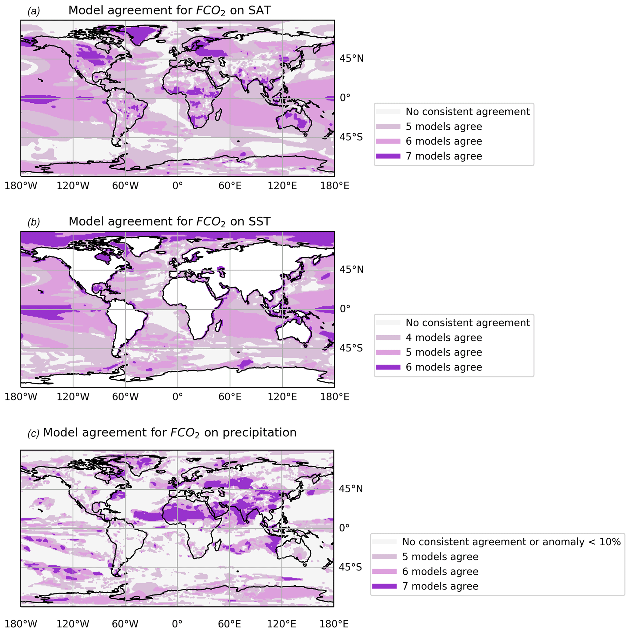
Figure 7 The level of agreement between models included in the FCO₂ analysis, showing where models agree on the dominant forcing shown by the FCO₂ method (i.e. whether FCO₂>0.5 or FCO₂<0.5). All seven models (CCSM4-UoT, CESM2, COSMOS, HadCM3, IPSLCM5A2, MIROC4m, and NorESM1-F) are included for the SAT and precipitation analysis; IPSLCM5A2 is excluded from the SST analysis, as only 10 model years of data were available – hence, a maximum of six models in agreement for SST. For precipitation, agreement is only assessed in regions where the Eoi⁴⁰⁰–E²⁸⁰ precipitation anomaly is greater than 10 % for consistency.

There is consistent agreement between five or more models on the dominant forcing of SAT over 74.8 % of the Earth's surface (Fig. 7a), of SST over 46.5 % of the ocean surface (Fig. 7b), and of precipitation over 66.8 % of regions with an Eoi⁴⁰⁰–E²⁸⁰ anomaly greater than 10 % (Fig. 7c). If the criteria for consistency are extended to four or more models for SST – for which only six models are assessed – the area in agreement increases to 83.1 %.

Although FCO₂ on precipitation is not the most consistent, in regions of agreement it is more common for all seven models to agree: all seven models agree on the dominant forcing over 13.8 % of the area assessed for precipitation compared to 4.6 % for SAT. All six models agree on the dominant forcing for SST over 11.4 % of the ocean surface.

4.2 Drivers of Pliocene climate

Using the FCO₂ method, CO₂ forcing was found to be the largest cause of SAT, SST, and precipitation change in the Pliocene, with global mean MMM FCO₂ values of 0.56, 0.56, and 0.51, respectively.

The percentage of SAT change predominantly driven by CO₂ using the FCO₂ method, 56 %, is comparable to estimates from previous studies, including specific comparisons for HadCM3 (Lunt et al., 2012), CCSM4-UoT (Chandan and Peltier, 2018), and COSMOS (Stepanek et al., 2020), as well as the PlioMIP1 ensemble (Hill et al., 2014).

Lunt et al. (2012) concluded that 48 % of warmth simulated in HadCM3 was caused by CO₂ when the atmospheric concentration was set to 400 ppm, decreasing to 36 % at 350 ppm and increasing to 61 % at 450 ppm. Exploring the effect of different atmospheric CO₂ concentrations in this way would be possible using the FCO₂ method but is constrained by the experiments set out in the PlioMIP2 experimental design; further division of forcing factorisation experiments and/or more models conducting these experiments (particularly the separated Eo⁴⁰⁰ and Ei⁴⁰⁰ experiments) may be a fruitful addition to PlioMIP3.

Using the FCO₂ method, 59 % of the Pliocene SAT anomaly is caused by CO₂ in HadCM3 (global mean FCO₂=0.59; Fig. S2d). This is higher than the estimate of 48 % in Lunt et al. (2012), but it is important to note the development in boundary conditions from PRISM2 (used in Lunt et al., 2012) to PRISM4 (used in PlioMIP2), which will account for some of the difference, as well as the difference in methodology.

The percentage of warming predominantly caused by CO₂ using the FCO₂ method in CCSM4-UoT, 52 % (global mean FCO₂=0.52; Fig. S2a), is also higher than the ∼45 % estimated in Chandan and Peltier (2018) using the nonlinear factorisation methodology of Lunt et al. (2012).

On the other hand, the FCO₂ method slightly underestimates the contribution of CO₂ in COSMOS compared to the full factorisation in Stepanek et al. (2020). The global mean FCO₂ for COSMOS is found to be 0.64 (64 % CO₂ contribution equivalent; Fig. S2c) compared to 66 % in Stepanek et al. (2020). This may reflect the incorporation of some vegetation feedback in the E⁴⁰⁰–E²⁸⁰ anomaly used to calculate FCO₂, given that COSMOS ran with dynamic vegetation, but additional simulations of COSMOS using prescribed vegetation would be needed to explore this further.

In validating the FCO₂ method, this paper has also presented the first energy balance results for a subgroup of models in the PlioMIP2 ensemble. By using the same methodology as Hill et al. (2014) in the framework of PlioMIP1, our results based on PlioMIP2 experiments become directly comparable, and similar trends are seen: greenhouse gas emissivity is dominant in driving warming in the tropics, while all forcing components become important in the high latitudes, with polar amplification particularly driven by clear-sky albedo. The relative dominance of CO₂ forcing in the low and mid-latitudes compared to in the high latitudes is also seen in the FCO₂ results.

We find notable variation of results based on the FCO₂ method between individual climate models, although the level of variation is consistent between the three climate variables assessed. Despite having the highest ECS value in the PlioMIP2 ensemble (5.3 ^∘C; Gettelman et al., 2019; Haywood et al., 2020), CESM2 has the lowest FCO₂ for all three variables at 0.40 for SAT and SST and 0.39 for precipitation (Figs. S2b, S3b, and S4b, respectively). This further highlights the sensitivity of CESM2 to all changes in boundary conditions and not just to CO₂ (Feng et al., 2020).

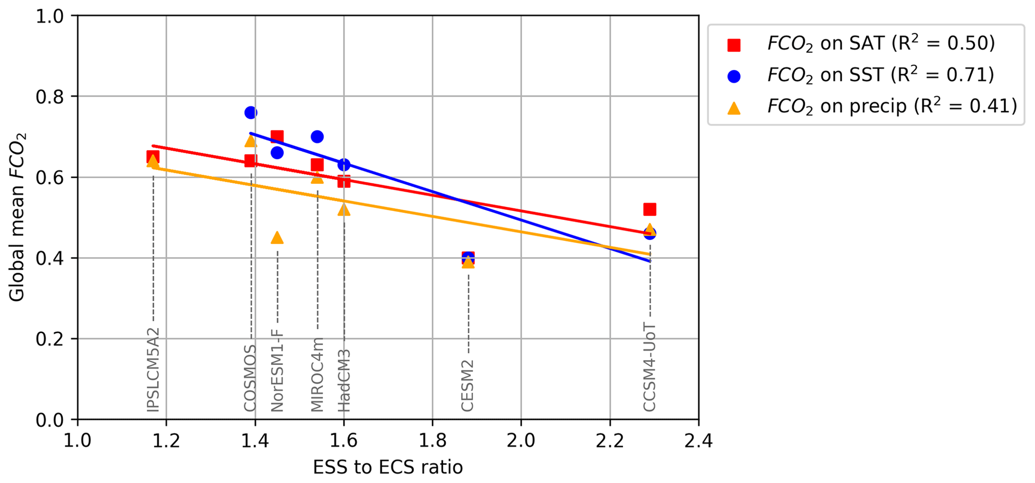
Figure 8 The relationship between the ESS-to-ECS ratio and global mean FCO₂. IPSLCM5A2 is excluded from the SST analysis due to limited data availability.

The model with the highest global mean FCO₂ differs between variables. NorESM1-F has the highest FCO₂ on SAT at 0.70 (Fig. S2), while COSMOS has the highest FCO₂ on SST and precipitation at 0.76 and 0.69, respectively (Figs. S3 and S4, respectively). NorESM1-F has the lowest ECS value in the PlioMIP2 ensemble (2.3 ^∘C), but COSMOS has the third highest (4.7 ^∘C; Haywood et al., 2020). Though it might seem intuitive that models with a higher ECS would also have a higher FCO₂, the relationship between FCO₂ and climate sensitivity can be better described by the ESS-to-ECS ratio, which captures the relatively short-term influence of CO₂ compared to longer-term responses of the Earth system (Fig. 8). Perhaps an artefact of the reduced sample size (six models compared to seven), the ESS-to-ECS ratio correlates best with the global mean FCO₂ on SST (R²=0.71), followed by SAT (R²=0.50) and precipitation (R²=0.41). This relationship would be better explored with a greater sample size, again reinforcing the usefulness of model groups completing the forcing factorisation experiments ahead of PlioMIP3.

4.3 The Pliocene as an analogue for the future?

A significant motivation behind studying the Pliocene is its use as a potential palaeoclimate analogue for the near-term future. If the Pliocene is to be an accurate and useful analogue for the future, it stands that the drivers of its climate should also be analogous to those driving current anthropogenic climate change alongside its large-scale climate features.

The FCO₂ method allows us to answer the question of how analogous the drivers of Pliocene climate are to those of the near-term future in more detail than has been possible previously. It also allows us to consider this question in terms of SST and precipitation change for the first time.

Current warming is predominantly driven by anthropogenic greenhouse gas emissions (Eyring et al., 2021). The FCO₂ results presented here show that, although CO₂ was the most important forcing in the Pliocene, it drove only 56 % of SAT and SST change and 51 % of precipitation change in the ensemble of PlioMIP2 models considered in this study. Therefore, 44 % of SAT and SST change and 49 % of precipitation change were driven by non-CO₂ forcing.

While we are already experiencing some shifts towards a Pliocene-like state for some of these non-CO₂ components – such as the greening of the Arctic (e.g. Myers-Smith et al., 2020) – other changes will take longer to fully materialise as the system equilibrates to higher levels of anthropogenic CO₂ forcing, with implications for the accuracy and utility of the Pliocene as a palaeoclimate analogue for near-term future climate. Regions of high FCO₂ in the Pliocene are likely to be more analogous for the immediate and near-term future for as long as the atmospheric CO₂ concentration remains similar to Pliocene levels (∼400 ppm), whereas regions of lower FCO₂ may become more analogous in the longer-term future as the full, equilibrated effects of changes to ice sheets and vegetation are experienced.

This raises two important points. The first highlights the importance of understanding the broader Earth system feedbacks of an atmospheric CO₂ concentration similar to modern, particularly as anthropogenic greenhouse gas emissions continue to increase (Dhakal et al., 2022), with the likelihood of soon moving beyond Pliocene levels (∼400 ppm; Meinshausen et al., 2020). The E⁴⁰⁰–E²⁸⁰ SAT anomaly shows that, for the subgroup of seven PlioMIP2 models assessed here, CO₂ forcing alone was responsible for 1.8 of the total 3.2 ^∘C increase seen in the Eoi⁴⁰⁰–E²⁸⁰ global mean SAT anomaly. We have experienced around 1.1 ^∘C of warming relative to the PI, with an atmospheric CO₂ concentration of around 410 ppm (Gulev et al., 2021). The Pliocene – being around 3 ^∘C warmer than the PI in quasi-equilibrium with a CO₂ concentration ∼400 ppm (e.g. Haywood et al., 2020) – shows that more warming is to come as the system equilibrates with the anthropogenic greenhouse gas forcing that has already been emitted, even if greenhouse gas emissions were to stop immediately.

The second point highlights the need to define what we mean by palaeoclimate analogue in the situation of our research. This should include consideration of the climate variable(s), region(s), and time frame(s) of interest (including whether the system is in a transient or equilibrium state, with implications for modes of variability, e.g. Bonan et al., 2022), as well as the level of accuracy deemed to be analogous. Our results also highlight the need to consider the nature of the climate forcing.

Burke et al. (2018) explore the spatial and temporal variations of past warm periods as analogues for different potential climate futures by comparing six geohistorical periods (PI, Historical, Holocene, Last Interglacial, Pliocene, and Eocene) to representative concentration pathway (RCP) 4.5 and RCP8.5. They find the Pliocene to be the best analogue for our near-term future under RCP4.5, although just because the Pliocene is one of the best palaeoclimate analogues does not necessarily mean that it is a perfect analogue without constraints or limitations.

Future work could expand the work of Burke et al. (2018) using the FCO₂ method to incorporate additional climate variables, which would also allow for discussion on the analogous nature of the drivers of these variables.

The results presented here highlight that, although there may be similarities in large-scale features of Pliocene and near-term future climate, the drivers of these features may be less similar or analogous, and drawing any such conclusions must be done with caution and should account for the significant contributions of non-analogous forcings.

5 Summary and future work

We have introduced a novel method for assessing the influence of different forcing factors in the Pliocene. The FCO₂ method only requires a small subset of forcing factorisation experiments of PlioMIP2 and can be applied to multiple climate variables and to a large ensemble of models with little computational complexity and cost. We have validated the FCO₂ method by comparing the results for SAT to an energy balance analysis using the methodology of Hill et al. (2014), which was originally used to assess the drivers of warming in the PlioMIP1 ensemble.

For the first time, we have quantitatively estimated the effect of CO₂ forcing on Pliocene SST and precipitation. CO₂ is found to be the most important forcing of global mean SAT, SST, and precipitation, with global mean FCO₂ values of 0.56 (individual model range 0.40–0.70), 0.56 (individual model range 0.40–0.76), and 0.51 (individual model range 0.39–0.69) respectively. Although CO₂ is the most important forcing, there remains significant contributions from non-CO₂ forcing, and such changes in orography, ice sheets, and/or vegetation are found to have a greater impact on driving regional spatial changes. The influence of these non-CO₂ forcings must not be overlooked, particularly in the context of using the Pliocene as an analogue for the near-term future.

Outputs from the FCO₂ method also provide new insights relevant to the palaeo-data community which could aid the interpretation of proxy data and data–model comparison efforts and could also inform estimates of climate sensitivity. These insights will be explored in a future paper. The FCO₂ method shows us which regions of the world are most (and least) influenced by CO₂ forcing, with direct implications for the interpretation of proxy data at these sites and any biases they may present. Additionally, we can also use the outputs from the FCO₂ method to suggest regions from which additional proxy data would be useful to further refine our interpretation of Pliocene climate, such as where there is uncertainty between models.

As we look towards the planning of PlioMIP3, our work clearly highlights the usefulness and importance of including forcing factorisation experiments that can provide us with a more detailed view of the drivers of Pliocene climate, with direct relevance to the discussion on using the Pliocene as an analogue for our warmer future.