the Creative Commons Attribution 4.0 License.
the Creative Commons Attribution 4.0 License.
 | 31 Mar 2023
How changing the height of the Antarctic ice sheet affects global climate: a mid-Pliocene case study
Xiaofang Huang
Shiling Yang
Alan Haywood
Julia Tindall
Dabang Jiang
Yongda Wang
Minmin Sun
Shihao Zhang
Warming-induced topographic changes of the East Antarctic ice sheet (EAIS) during the Pliocene warm period could have a significant influence on the climate. However, how large changes in the EAIS height could theoretically affect global climate have yet to be studied. Here, the influence of possible height changes of the EAIS on climate over the East Antarctic ice sheet region versus the rest of the globe is investigated through numerical climate modeling using the Pliocene as a test case. As expected, the investigation reveals that the reduction of ice sheet height leads to a warmer and wetter East Antarctica. However, unintuitively, both the surface air temperature and the sea surface temperature decrease over the rest of the globe. These temperature changes result from the higher air pressure over Antarctica and the corresponding lower air pressure over extra-Antarctic regions with the reduction of EAIS height. This topography effect is further confirmed by energy balance analyses. These findings could provide insights into future climate change caused by warming-induced height reduction of the Antarctic ice sheet.
- Article
(13999 KB) - Full-text XML
-
Supplement
(1259 KB) - BibTeX
- EndNote


The Antarctic ice sheet (AIS) is the largest component (by volume) of Earth's cryosphere (Gasson and Keisling, 2020). It accounts for almost 70 % of the world's freshwater, representing a potential sea level rise of 56.6 m (Shum et al., 2008). Its evolution has received considerable attention in climate research, as it determines the surface mass balance that has a major impact on both regional and global climate (DeConto et al., 2007; Bintanja et al., 2013; Goldner et al., 2014; Colleoni et al., 2018; Golledge et al., 2019; Tewari et al., 2021a). The size of the present-day AIS is known to impinge substantially on synoptic- and planetary-scale atmospheric flow (Parish and Bromwich, 2007; Schmittner et al., 2011; Hakuba et al., 2012; Goldner et al., 2013; Grazioli et al., 2017), and in turn, the warming-induced topographic changes of the AIS have a significant influence on the climate (Orr et al., 2008; Tewari et al., 2021a, b). However, the effect of the AIS height changes on future predictions of climate is still uncertain. One method of investigating this effect in a warmer-than-modern climate is to look back at past warm periods of Earth's history, for example the Pliocene.
The mid-Pliocene warm period (∼3.3–3.0 Ma) is the most recent period of relatively warm and stable climate in Earth's history, during which atmospheric CO2 concentrations were approximately 400 ppmv (Pagani et al., 2010; Lunt et al., 2012b; Yang et al., 2018; De La Vega et al., 2020; Huang et al., 2021), and models have suggested that the global mean annual temperature was 1.7–5.2 ∘C warmer than today (Haywood et al., 2020). This period is similar to today in terms of the continent–ocean configuration and atmospheric CO2 concentrations (Haywood et al., 2016), and it has often been proposed as a climatic analog for the end of this century (Burke et al., 2018). The present atmospheric CO2 concentration is over 410 ppmv and has reached the Pliocene level. However, due to the large thermal inertia of the oceans (Levitus et al., 2000; Back et al., 2013), the atmosphere–ocean system is still in a nonequilibrium state, and the global mean temperature is projected to rise to the level of the Pliocene as early as the 2040s (Zhang, 2012; Ding et al., 2014; Burke et al., 2018; Tierney et al., 2020). In this scenario, about 30 % of the Antarctic mass loss amounts will occur in coming centuries (Grant et al., 2019). Therefore, we use climate model simulations of the Pliocene to investigate how large, hypothetical changes in East AIS (EAIS) height would affect the climate.
Numerical experiments have emerged as an efficient means of understanding past climates on regional and global scales (Huang et al., 2019). Based on simulations, the dynamic behavior of the AIS and its stability in relation to climate change have been analyzed (Raymo et al., 2006; Naish et al., 2009; Cook et al., 2013; Patterson et al., 2014; Austermann et al., 2015; Boer et al., 2015; Yamane et al., 2015; Scherer et al., 2016; Dolan et al., 2018). Here, we design sensitivity experiments using a coupled climate model to investigate how perturbations in the EAIS height would interact with the atmospheric flow and influence the temperature and precipitation dynamics over the East Antarctic ice sheet region and the rest of the globe.
2.1 Model description
The Hadley Centre coupled climate model version 3 (hereafter referred to as HadCM3) was used for this study. This model has been used extensively for studies of the Pliocene within the Pliocene Model Intercomparison Project experiments (Haywood et al., 2010, 2011; Bragg et al., 2012; Hunter et al., 2019). HadCM3 consists of two main components: an atmospheric component (HadAM3) and an oceanic component (HadOM3; Gordon et al., 2000; Pope et al., 2000; Valdes et al., 2017). The horizontal resolution of the atmosphere model is 2.5∘ in latitude by 3.75∘ in longitude, and it consists of 19 layers vertically. The atmospheric model has a time step of 30 min and includes a radiation scheme that can represent the effects of major and minor trace gases (Edwards and Slingo, 1996). The spatial resolution of the HadOM3 oceanic model is 1.25∘ latitude by 1.25∘ longitude, with 20 vertical layers. The ocean model is a rigid-lid model, which has a time step of 1 h and incorporates a thermodynamic–dynamic sea ice model with primitive (ocean drift) dynamics. The HadCM3 has been shown to represent well the broad-scale features of the Antarctic and Arctic atmospheric and oceanic circulation (Turner et al., 2006; Chapman and Walsh, 2007). The fact that the HadCM3 consistently performs well in tests against other coupled atmosphere–ocean models (Lambert and Boer, 2001; Hegerl et al., 2007; Dolan et al., 2011) increases our confidence in its paleoclimate simulations.
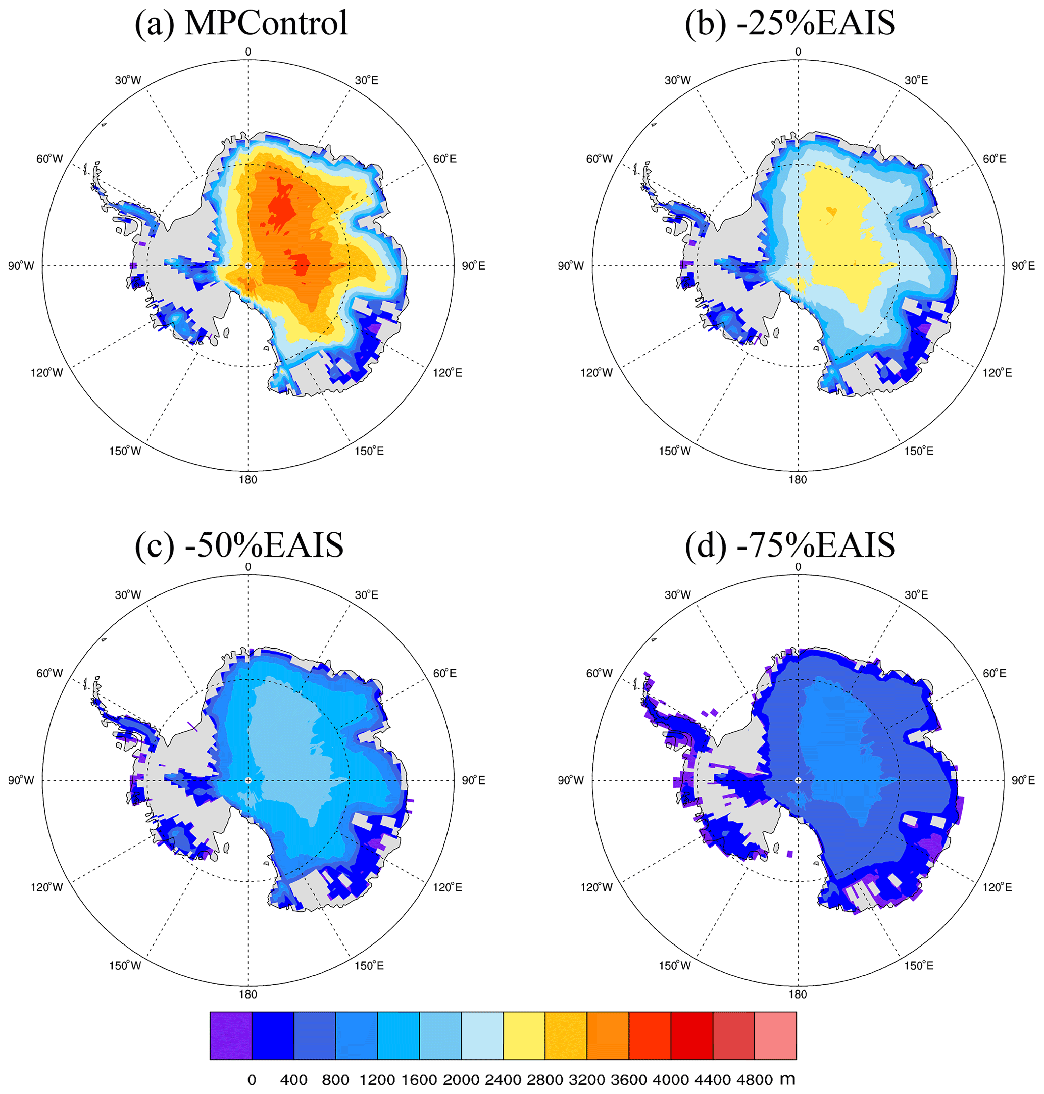
Figure 1The height of the East Antarctic ice sheet for the (a) mid-Pliocene control experiment, (b) −25 % EAIS sensitivity experiment, (c) −50 % EAIS sensitivity experiment, and (d) −75 % EAIS sensitivity experiment. It should be noted that, for the −100 % EAIS sensitivity experiment, the height of the East Antarctic ice sheet has been set to zero, while the surface type is still snow.
2.2 Pliocene boundary conditions and experimental designs
For this study, the required mid-Pliocene boundary conditions were supplied by the US Geological Survey Pliocene Research Interpretations and Synoptic Mapping Group's (PRISM) dataset, specifically the latest iteration of the reconstruction known as PRISM4 (Dowsett et al., 2016). They include topography and bathymetry, coastlines, land surface properties (i.e., vegetation, soil type, and ice sheet coverage), and atmospheric composition with respect to pre-industrial conditions. The Greenland ice sheet and the West Antarctic ice sheet, which currently store ∼13 m of sea-level-equivalent ice (Dolan et al., 2011; Yamane et al., 2015), are thought to have largely melted during the mid-Pliocene warm period (Lunt et al., 2008; Naish et al., 2009). Therefore, our experiments focus on changing the East Antarctic ice sheet height (Fig. 1) in relation to its reconstructed Pliocene value. It should be noted that the surface type is still snow, and so there will still be high albedo in this region.
Our control simulation is started from the end of the HadCM3 contribution to the PlioMIP2 simulation (Hunter et al., 2019). There is a difference between our control simulation and the PlioMIP2 simulation; namely, we use dynamic vegetation, while Hunter et al. (2019) use fixed vegetation from PRISM4. we manipulate the height of the ice sheet for each sensitivity simulation on the basis of the control experiment. To evaluate the regional and global climate sensitivity to the EAIS height changes, five Pliocene modeling experiments are presented in this paper. These experiments were identical except with regard to the height of the EAIS – specifically, we present one mid-Pliocene control run (hereafter MPControl) and four sensitivity simulations with the EAIS height reduced by 100 % (hereafter −100 % EAIS), 75 % (hereafter −75 % EAIS), 50 % (hereafter −50 % EAIS), and 25 % (hereafter −25 % EAIS) of the Pliocene height. All these sensitivity experiments are hypothetical scenarios and are not intended to correspond to projected future scenarios. Instead, they are designed to isolate how changes in the elevation of the EAIS would affect a warmer world.
To provide a more realistic −100 % EAIS experiment, we further performed an experiment in which the EAIS is still at −100 %, but the land topography (away from Antarctica) is reduced by 60 m (hereafter −100 % EAIS and −60 m land) to artificially raise the sea level. Locations where the land was below 60 m are set to 0 m to maintain the mid-Pliocene land–sea mask, which means that there are no ocean gateway changes that could affect ocean dynamics.
The mid-Pliocene control experiment uses the East Antarctic ice sheet configuration (and all other boundary conditions) specified in the USGS PRISM4 data set. The EAIS volume is smaller during the mid-Pliocene than at present, and the reduced EAIS is equivalent to 15 m sea level rise (Dowsett et al., 2010). All experiments (including the ice sheet sensitivity experiments) are started from the end of the HadCM3 PlioMIP2 simulation and are continued for another 500 model years, allowing the modeled climate to be equilibrated to the boundary conditions. Climate statistics are based on time averages of the final 30 years for each run. The results are presented as anomalies of the control for the sensitivity experiments.
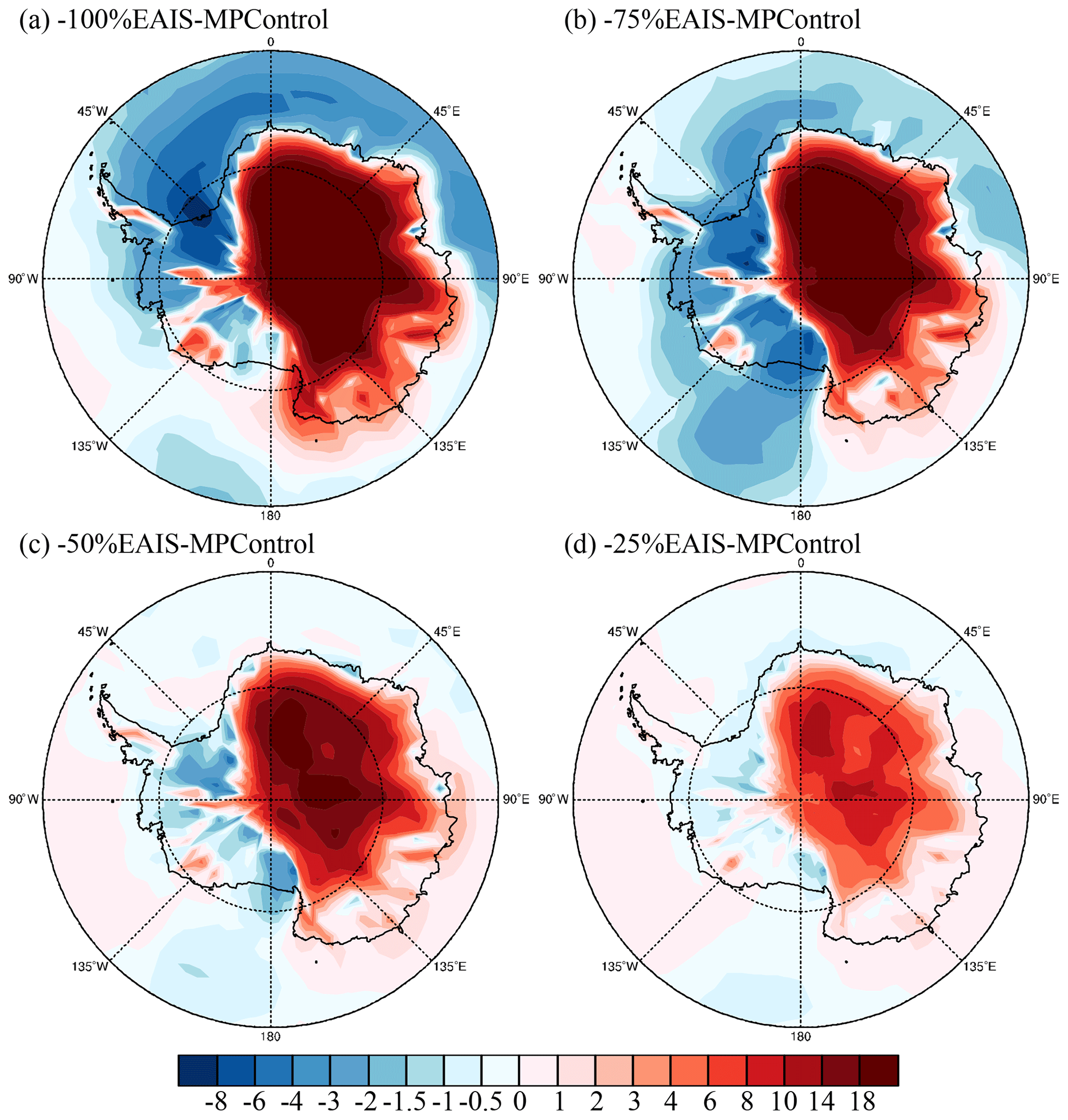
Figure 2Spatial distribution of the annual mean surface temperature anomalies (units: ∘C) over Antarctica between sensitivity experiments and MPControl experiments.
3.1 Surface air temperature changes
Reducing the height of the EAIS in our experiments results in a dramatic annual mean warming over East Antarctica relative to the MPControl experiment (Fig. 2). Compared with the MPControl experiment, the East Antarctic annual mean surface temperature increases by about 5, 10, 15, and 18 ∘C with height reductions of 25 %, 50 %, 75 %, and 100 %, respectively (Fig. 2). Based on Fig. 1a, the average height of the EAIS is ∼3.2 km, which means that every 25 % reduction of the height equates to ∼0.8 km. Clearly, this surface warming occurs at a rate of ∼6 of EAIS height lost, which is confirmed by the change in temperature due to changing surface height (Fig. S1 in the Supplement) and is accompanied by a prominent surface cooling over western Antarctica and the Southern Ocean.
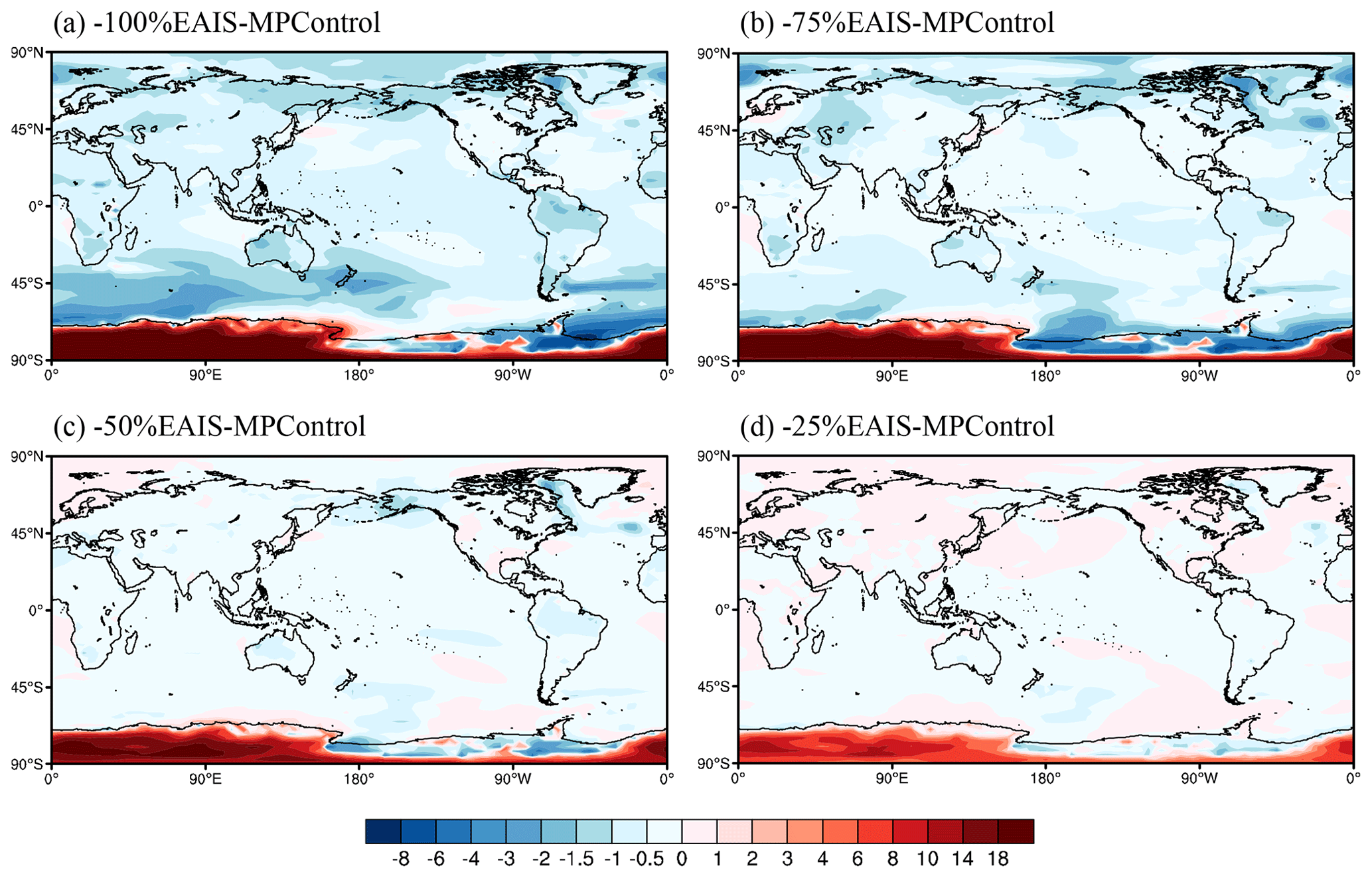
Figure 3Spatial distribution of the annual mean surface air temperature anomalies (units: ∘C) over the globe between sensitivity experiments and MPControl experiments.
Contrary to Antarctic warming, reducing the height of the EAIS leads to annual mean surface cooling over the rest of the globe (Fig. 3). The inclusion of the −100 % EAIS set of boundary conditions results in a ∼1–2 ∘C mean cooling over the rest of the globe (Fig. 3a). In low and equatorial regions, temperatures decrease by a minimum of 0.5–1 ∘C, and cooling is at its greatest (∼3 ∘C) over Southern Ocean. For the −75 % EAIS and −50 % EAIS experiments (Fig. 3b and c), annual mean values for surface air temperature decrease by ∼0.5 and ∼1 ∘C, respectively. Compared with the MPControl experiment, the surface air temperature in the −25 % EAIS experiment changes little (the mean value is near zero; Fig. 3d).
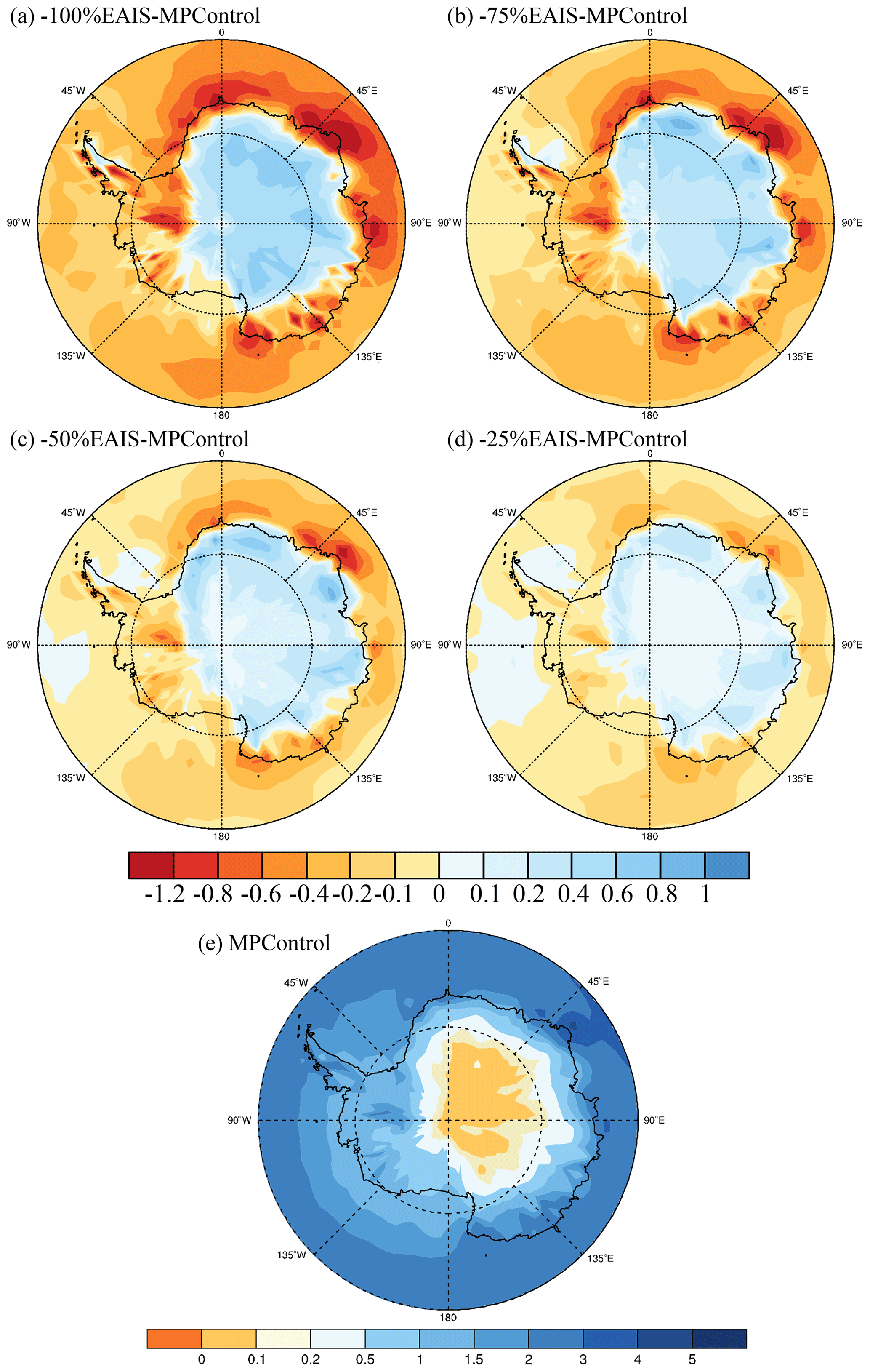
Figure 4Spatial distribution of the annual mean precipitation anomalies (units: mm d−1) over Antarctica between sensitivity experiments and MPControl experiments (a–d), and spatial distribution of the annual mean precipitation over Antarctica for the MPControl experiments (e).
3.2 Precipitation changes
The numerical simulations show that, with the height reduction of the EAIS, the annual precipitation increased over East Antarctica and decreased over the rest of the Southern Hemisphere (Fig. 4). Precipitation enhancements are greatest in −100 % EAIS (∼0.4 mm d−1; Fig. 4a) and smallest in −25 % EAIS (∼0.1 mm d−1; Fig. 4d). Based on Fig. 4e, the annual mean precipitation of the MPControl experiment over the EAIS is ∼0.4 mm d−1, which means that the precipitation increases by ∼25 % with every 25 % reduction of the height. Clearly, this precipitation enhancement over East Antarctica occurs at a rate of approximately 5 % per degrees Celsius, which is accompanied by a precipitation deficit over western Antarctica and the Southern Ocean. With respect to the MPControl experiment, precipitation reduces significantly over western Antarctica and the Southern Ocean (∼0.3–0.8 mm d−1; Fig. 4a) in the −100 % EAIS experiments but decreases slightly over those areas (∼0.1–0.2 mm d−1; Fig. 4d) in the −25 % EAIS experiments.
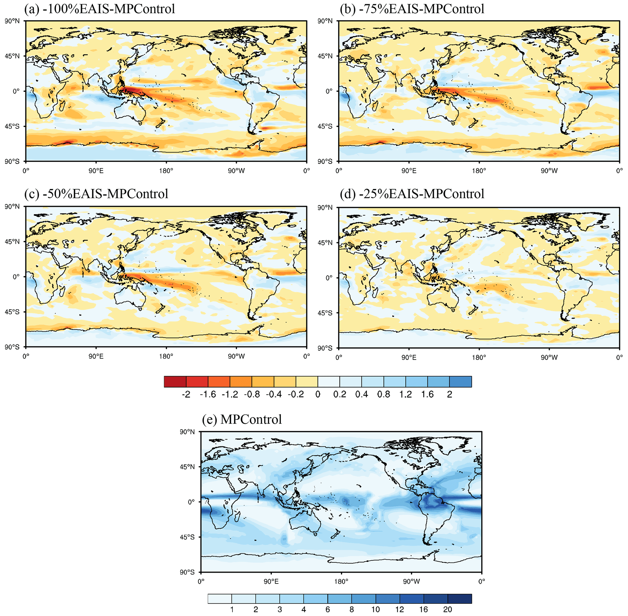
Figure 5Spatial distribution of the annual mean precipitation anomalies (units: mm d−1) between sensitivity experiments and MPControl experiments (a–d), and spatial distribution of the annual mean precipitation for the MPControl experiments (e).
Annual precipitation decreases consistently over most areas globally in all the sensitivity experiments compared to in the MPControl experiments (Fig. 5). This is consistent with the decreased air temperatures (Fig. 3), which reduce the moisture-carrying capacity of the air and lead to less precipitation. The experiment that shows the greatest sensitivity in terms of precipitation response is −100 % EAIS, with the anomaly varying from −2 to 0.8 mm d−1 (Fig. 5a), while the experiment that shows the least sensitivity is −25 % EAIS, with a narrow anomalous range of −0.4–0.4 mm d−1 (Fig. 5d). The spatial patterns (Fig. 5a–d) show that the enhanced precipitation is focused over parts of the tropics and the 45th parallel south, while the deficit is focused over northern high latitudes and the Antarctic periphery. The largest precipitation anomaly is found in the tropics, which are dominated by the Intertropical Convergence Zone (ITCZ). In general, for most areas except the Southern Ocean, the simulations that display the largest surface air temperature sensitivity to the prescription of EAIS height changes also exhibit the largest precipitation anomalies.
4.1 Cause of the precipitation changes over Antarctica
Earlier studies have shown a clear relationship between the atmospheric circulation and precipitation dynamics, arguing that precipitation over polar regions is mostly due to orographic effects acting upon the circulation pattern passing over the region (Schmittner et al., 2011; Hakuba et al., 2012; Goldner et al., 2013; Tewari et al., 2021a). The mechanical obstruction by the ice sheet prevents the moisture-laden winds from penetrating inland (Parish and Bromwich, 2007; Grazioli et al., 2017; Tewari et al., 2021b). The gravity-driven katabatic flow, which carries dense cold air masses out from the polar plateau, impedes a poleward shift of the moisture-laden winds (Goldner et al., 2013; Tewari et al., 2021b). Therefore, the weakened katabatic flow, due to the successive topographic reduction, leads to an elevated moisture transport into the continent (Fig. 7), thereby increasing precipitation over the EAIS (Fig. 4).

Figure 6Annual mean wind circulation at 850 hPa over the Southern Hemisphere (a; units: m s−1) and its corresponding anomalies in −100 % EAIS, −75 % EAIS, −50 % EAIS, and −25 % EAIS, respectively (b–e; units: m s−1).
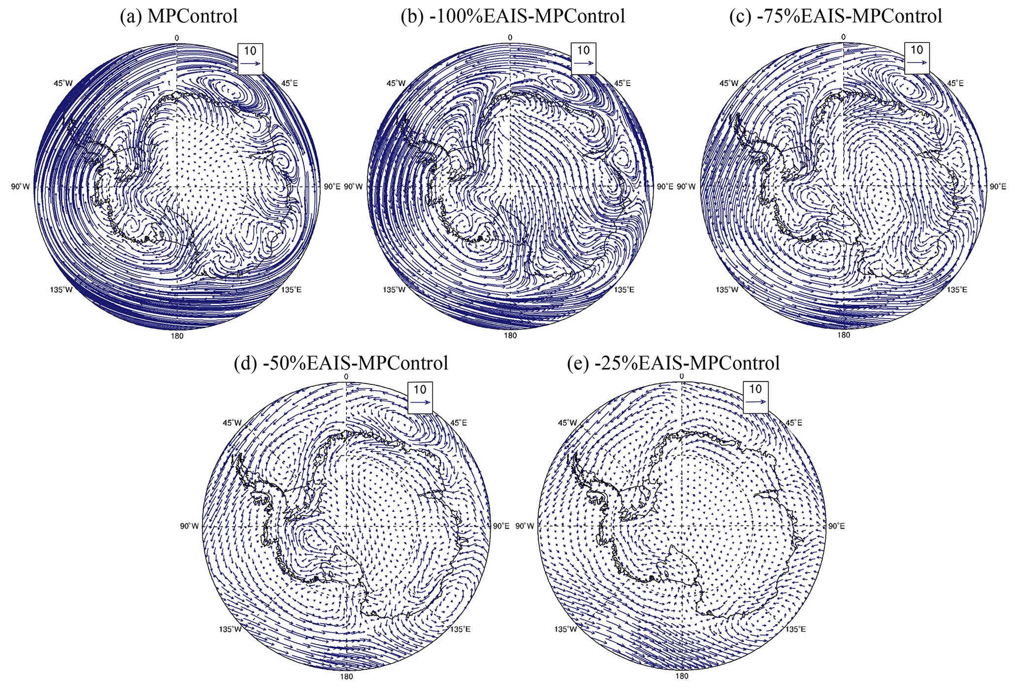
Figure 7Vertically integrated water vapor flux over Antarctica (arrows; units: ) for (a) the MPControl, and the anomalies (arrows; units: ) for (b) the −100 % EAIS relative to the MPControl, (c) the −75 % EAIS relative to the MPControl, (d) the −50 % EAIS relative to the MPControl, and (e) the −25 % EAIS relative to the MPControl.
Figure 6 shows the magnitude and direction of the low-level winds at 850 hPa over the Southern Hemisphere and the corresponding changes observed in their strength due to orographic perturbations in individual simulations. In the MPControl experiment, strong surface westerly winds encircle the East Antarctic continent, extending from ∼60∘ S to the continental periphery (Fig. 6a), indicating the blocking effect of the EAIS (Tewari et al., 2021b).
Upon successive reduction of the EAIS height (Fig. 6b–e), the westerly flow becomes weaker between 60 and 90∘ S and penetrates gradually into the eastern continent. The EAIS height reductions of 100 % and 75 % cause a poleward shift in the surface flows (Fig. 6b and c), which even circulate around the South Pole. In contrast, reductions by 50 % and 25 % cause little change in the surface winds. In this context, sustained attention needs to be paid to changes in the height of the AIS in relation to future warming, as well as to the effect of these changes on atmospheric circulation and precipitation dynamics over the region.
To further investigate the mechanism for the precipitation changes over Antarctica, we analyzed the annual water vapor flux over this region. The results show that, in the MPControl experiment, strong westerly flows encircle the East Antarctic continent, extending from ∼60∘ S to the continental periphery (Fig. 7a). In contrast, with the height reduction of the EAIS, the anomalies show easterly flows that encircle the East Antarctic continent, extending from ∼60∘ S to the continental periphery (Fig. 7b–e). These flows mean that the water vapor flux decreases over the region, from ∼60∘ S to the continental periphery, which is consistent with the decreased precipitation over this region (Fig. 4). Over East Antarctica, upon successive reduction of the EAIS height, the westerly flow penetrates gradually into the eastern continent and brings more and more water vapor into this region (Fig. 7b–e), which is consistent with the increased precipitation over the eastern continent (Fig. 4).
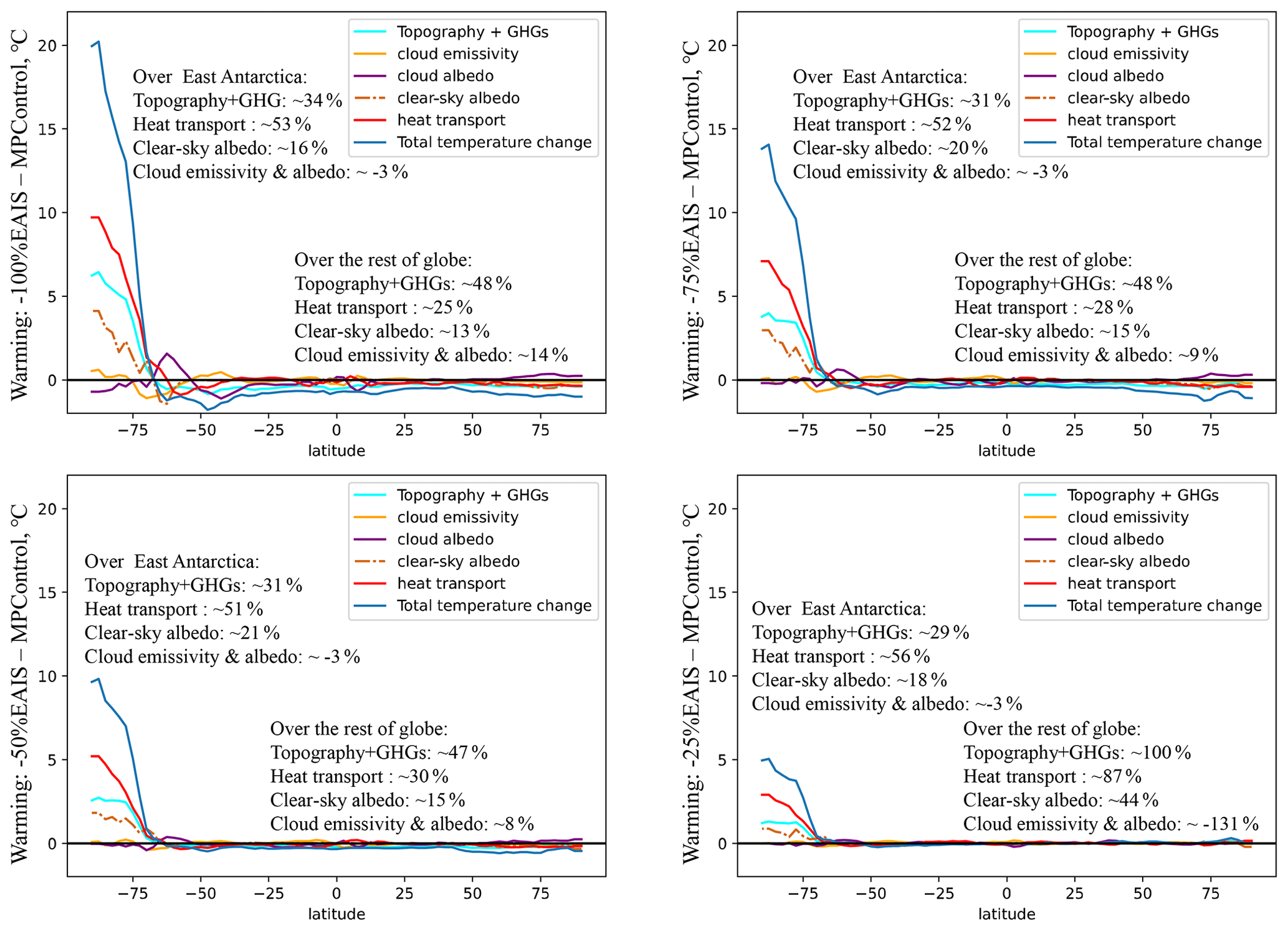
Figure 8Energy balance analysis between the sensitivity experiments and the MPControl. Plot shows the zonal mean warming and cooling at each latitude from each of the energy balance components. GHGs stands for greenhouse gases. The percentage value represents the contribution of each energy balance component to the temperature changes over East Antarctica and the rest of globe.
4.2 Causes of global temperature changes
In order to identify factors controlling the air temperature changes with the height reductions of the EAIS, energy balance analyses (Heinemann et al., 2009; Lunt et al., 2012a; Hill et al., 2014) between the sensitivity experiments and the MPControl experiment have been completed. This approach has been used in paleoclimate simulations to understand the simulated temperature changes (Donnadieu et al., 2006; Murakami et al., 2008; Hill et al., 2014; Lunt et al., 2021; Baatsen et al., 2022), and more details about how to conduct this energy balance analysis can be found in Hill et al. (2014). The results show that the heat transport from the rest of the globe, especially from the proximal Southern Ocean, to Antarctica is the primary factor influencing the temperature changes over Antarctica, with its contribution rate reaching ∼52 % (Fig. 8). However, over the rest of the globe, the heat transport is the secondary factor influencing the temperature decrease (Fig. 3), and except in the case of the −25 % EAIS experiment, its contribution in other sensitivity experiments reaches ∼25 % (Fig. 8).
The secondary factor controlling the Antarctic temperature is topography and GHGs (greenhouse gases), with their contribution rate reaching ∼30 % (Fig. 8). In contrast, over the rest of the globe, the primary factor influencing the temperature changes is topography and GHGs, with their contribution being ∼48 %. All experiments were forced with the same trace gases; therefore the “Topography + GHGs” factor in Fig. 8 represents both the direct effect of ice sheet height changes on temperature and some indirect effects via GHG feedbacks.
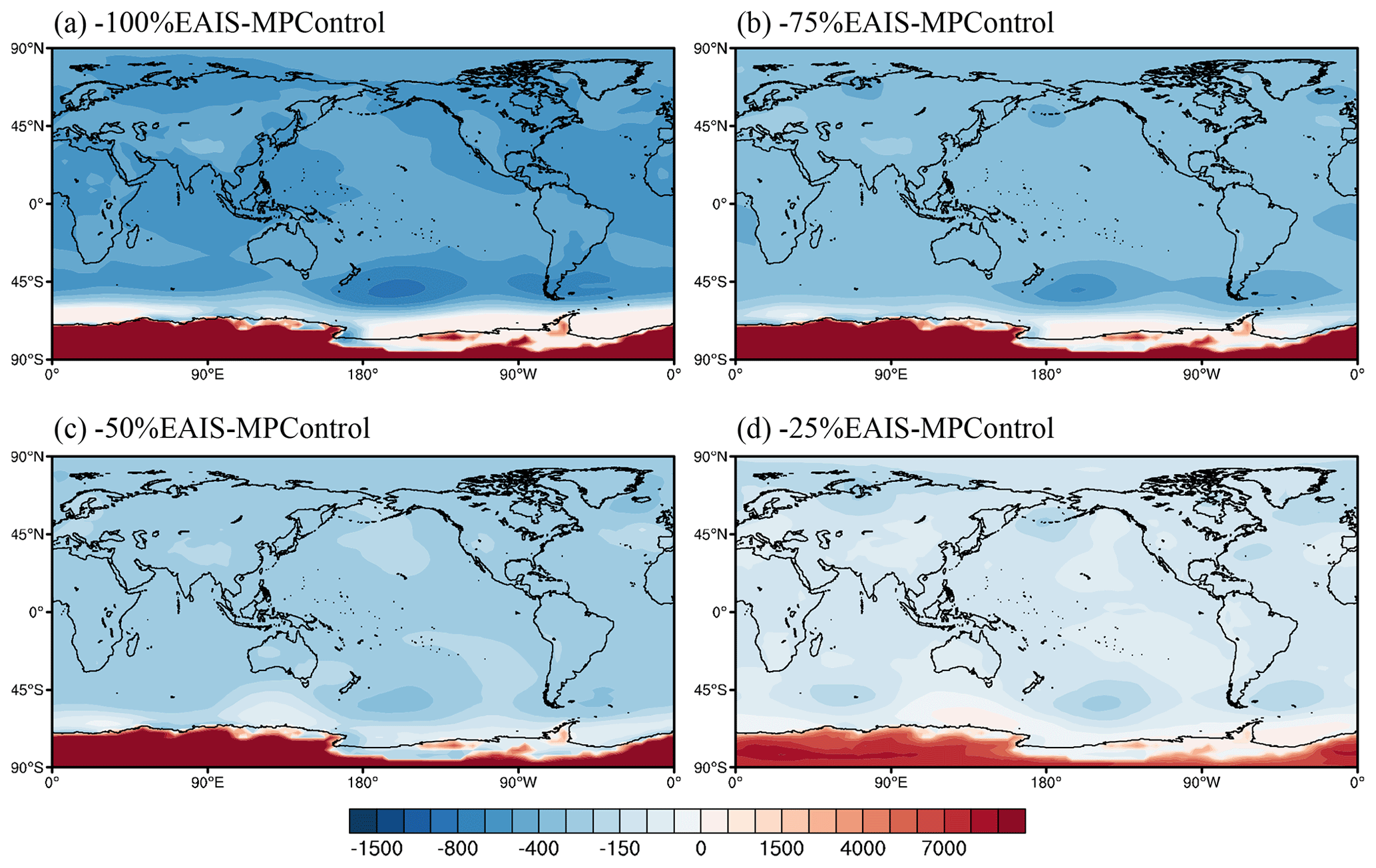
Figure 9Spatial distribution of the annual mean surface air pressure anomalies (units: Pa) between sensitivity experiments and the MPControl experiment.
The direct effect of ice sheet height changes on temperature can be explained by the surface air pressure changes. As shown in Fig. 9, the surface air pressure increases over Antarctica and decreases elsewhere, which is similar to the spatial pattern of the air temperature changes (Fig. 3). With the reduction of the EAIS height, the air mass increases over Antarctica at the expense of that over the rest of the globe, leading to higher air pressure over Antarctica and lower air pressure over extra-Antarctic regions (Fig. 9). According to the ideal gas law (Clapeyron, 1834), lower air pressures correspond with lower air temperatures, which may explain the temperature contrast between Antarctica and extra-Antarctic regions.
The possible indirect effects include the following: (1) when the EAIS is reduced, the atmosphere will become thicker in this region, which will lead to more greenhouse gases in the column and hence to more warming; and (2) the warmer atmosphere will be able to hold more water vapor. Our results are useful for a better understanding of the effect of the AIS height changes on climate.
4.3 Modeling methodological limitations
In the present study, the HadCM3 model was used to investigate the influence of the height reduction of the EAIS on temperature, precipitation, atmospheric circulation, surface air pressure, and the energy transport at regional and global scales. The objective of these simulations was to quantify how the existence of the EAIS would affect the mid-Pliocene climate. It can be concluded from the present findings that a reduction in the EAIS height during the mid-Pliocene warm period induces warming and wetting over East Antarctica and cooling over the extra-Antarctica regions. The Antarctic surface warming and coastal cooling due to the height reduction of the Antarctic ice sheet were also observed in the modern Antarctic height reduction sensitivity experiments using the CAM5.1 model (Tewari et al., 2021a). It should be noted that the effects of changes in the surface albedo, sea level, and continental margins, which would undoubtedly occur with such orographic variations, have not been explicitly taken into account in the present idealized simulations. Despite these caveats, we expect that the dynamical influence of the EAIS over the Antarctic presented herein will persist even in their presence.
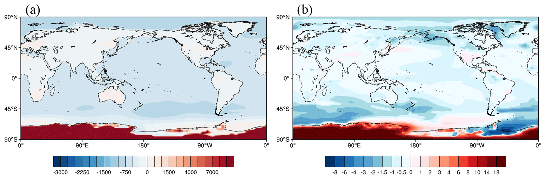
Figure 10Spatial distribution of (a) the annual mean surface air pressure anomalies (units: Pa) and (b) the annual mean surface air temperature (units: ∘C) between the new sensitivity experiment and the MPControl experiment. The new sensitivity experiment is similar to the −100 % EAIS experiment, except the sea level is artificially raised by a reduction of the land level (away from Antarctica) by 60 m.
Another modeling limitation is that the water contained in Antarctica did not get redistributed over the ocean when we reduced the EAIS height. This is because the HadCM3 is a rigid-lid model, which means the sea level is essentially fixed. The −100 % EAIS and −60 m land experiment enables an assessment of how pressure changes due to the loss of the EAIS will affect the global temperature (Fig. 10). The changes between this experiment and the MPControl experiment show that the surface air temperature and surface air pressure (Fig. 10) both show a similar spatial pattern to the changes between the −100 % EAIS and MPControl experiments. However, the results also show that (1) the pressure difference over the land (Fig. 10a) is much smaller than that in Fig. 9a, but there is still a pressure difference over the ocean; and (2) the temperature over the land away from Antarctica is still colder (Fig. 10b), although not by as much as that in Fig. 3a. Clearly, the cooling away from Antarctica is robust and would occur even if sea level changes were accounted for. Therefore, global temperature changes are likely to result from changes in the height of the EAIS.
The sensitivity of climate to the height changes of the East Antarctic ice sheet during the mid-Pliocene warm period has been assessed using the HadCM3 model. The results show that, due to a successive topographic reduction in the East Antarctic ice sheet, (i) the surface air temperature over the EAIS increases at a rate of approximately 6 of EAIS height lost, (ii) the precipitation over the EAIS increases at a rate of approximately 5 % per degree Celsius, (iii) the surface air temperature and the sea surface temperature both decrease over the rest of the globe, and (iv) the surface air pressure increases over East Antarctica and decreases elsewhere. Energy balance analyses show that the heat transport, which results from the topography changes of Antarctica, is mainly responsible for the temperature changes.
The data presented in the figures can be downloaded from the server located at the School of Earth and Environment of the University of Leeds. Contact Julia Tindall (j.c.tindall@leeds.ac.uk) for access.
The supplement related to this article is available online at: https://doi.org/10.5194/cp-19-731-2023-supplement.
XH contributed to the experiments, data analysis, conceptualization, and drafting of the paper. SY provided the funding acquisition. AH contributed to the experiment designs. JT assisted in performing the experiments. All the authors made contributions to the paper discussions and helped in revising the drafting of the paper.
The contact author has declared that none of the authors has any competing interests.
Publisher's note: Copernicus Publications remains neutral with regard to jurisdictional claims in published maps and institutional affiliations.
This study was supported by the National Natural Science Foundation of China (grant nos. 41725010 and 42107472), the Strategic Priority Research Program of the Chinese Academy of Sciences (grant nos. XDB26000000 and XDB31000000), and the Key Research Program of the Institute of Geology & Geophysics, CAS (grant no. IGGCAS-201905). The authors thank Steven Phipps, Michiel Baatsen, and one anonymous reviewer for their critical comments.
This research has been supported by the National Natural Science Foundation of China (grant no. 41725010), the National Natural Science Foundation of China (grant no. 42107472), the Strategic Pioneer Research Projects of Defense Science and Technology (grant no. XDB26000000), the Strategic Pioneer Research Projects of Defense Science and Technology (grant no. XDB31000000), and the Key Research Program of the Institute of Geology & Geophysics, CAS (grant no. IGGCAS-201905).
This paper was edited by Steven Phipps and reviewed by Michiel Baatsen and one anonymous referee.
Austermann, J., Pollard, D., Mitrovica, J. X., Moucha, R., Forte, A. M., DeConto, R. M., Rowley, D. B., and Raymo, M. E.: The impact of dynamic topography change on Antarctic ice sheet stability during the mid-Pliocene warm period, Geology, 43, 927–930, https://doi.org/10.1130/G36988.1, 2015.
Baatsen, M. L. J., von der Heydt, A. S., Kliphuis, M. A., Oldeman, A. M., and Weiffenbach, J. E.: Warm mid-Pliocene conditions without high climate sensitivity: the CCSM4-Utrecht (CESM 1.0.5) contribution to the PlioMIP2, Clim. Past, 18, 657–679, https://doi.org/10.5194/cp-18-657-2022, 2022.
Back, L., Russ, K., Liu, Z., Inoue, K., Zhang, J., and Otto-Bliesner, B.: Global hydrological cycle response to rapid and slow global warming, J. Climate, 26, 8781–8786, https://doi.org/10.1175/jcli-d-13-00118.1, 2013.
Bintanja, R., van Oldenborgh, G. J., Drijfhout, S. S., Wouters, B., and Katsman, C. A.: Important role for ocean warming and increased ice-shelf melt in Antarctic sea-ice expansion, Nat. Geosci., 6, 376–379, https://doi.org/10.1038/ngeo1767, 2013.
Bragg, F. J., Lunt, D. J., and Haywood, A. M.: Mid-Pliocene climate modelled using the UK Hadley Centre Model: PlioMIP Experiments 1 and 2, Geosci. Model Dev., 5, 1109–1125, https://doi.org/10.5194/gmd-5-1109-2012, 2012.
Burke, K. D., Williams, J. W., Chandler, M. A., Haywood, A. M., Lunt, D. J., and Otto-Bliesner, B. L.: Pliocene and Eocene provide best analogs for near-future climates, P. Natl. Acad. Sci. USA, 115, 13288–13293, https://doi.org/10.1073/pnas.1809600115, 2018.
Chapman, W. L. and Walsh, J. E.: Simulations of Arctic temperature and pressure by global coupled models, J. Climate, 20, 609–632, https://doi.org/10.1175/jcli4026.1, 2007.
Clapeyron, É.: Mémoire sur la puissance motrice de la chaleur, Journal de l'École polytechnique, 14, 153–190, 1834.
Colleoni, F., De Santis, L., Siddoway, C. S., Bergamasco, A., Golledge, N. R., Lohmann, G., Passchier, S., and Siegert, M. J.: Spatio-temporal variability of processes across Antarctic ice-bed–ocean interfaces, Nat. Commun., 9, 1–14, https://doi.org/10.1038/s41467-018-04583-0, 2018.
Cook, C. P., Van De Flierdt, T., Williams, T., Hemming, S. R., Iwai, M., Kobayashi, M., Jimenez-Espejo, F. J., Escutia, C., González, J. J., Khim, B., McKay, R. M., Passchier, S., Bohaty, S. M., Riesselman, C. R., Tauxe, L., Sugisaki, S., Galindo, A. L., Patterson, M. O., Sangiorgi, F., Pierce, E. L., Brinkhuis, H., Klaus, A., Fehr, A., Bendle, J. A. P., Bijl, P. K., Carr, S. A., Dunbar, R. B., Flores, J. A., Hayden, T. G., Katsuki, K., Kong, G. S., Nakai, M., Olney, M. P., Pekar, S. F., Pross, J., Röhl, U., Sakai, T., Shrivastava, P. K., Stickley, C. E., Tuo, S., Welsh, K., and Yamane, M.: Dynamic behaviour of the East Antarctic ice sheet during Pliocene warmth, Nat. Geosci., 6, 765–769, https://doi.org/10.1038/NGEO1889, 2013.
de Boer, B., Dolan, A. M., Bernales, J., Gasson, E., Goelzer, H., Golledge, N. R., Sutter, J., Huybrechts, P., Lohmann, G., Rogozhina, I., Abe-Ouchi, A., Saito, F., and van de Wal, R. S. W.: Simulating the Antarctic ice sheet in the late-Pliocene warm period: PLISMIP-ANT, an ice-sheet model intercomparison project, The Cryosphere, 9, 881–903, https://doi.org/10.5194/tc-9-881-2015, 2015.
DeConto, R., Pollard, D., and Harwood, D.: Sea ice feedback and Cenozoic evolution of Antarctic climate and ice sheets, Paleoceanography, 22, PA3214, https://doi.org/10.1029/2006pa001350, 2007.
De La Vega, E., Chalk, T. B., Wilson, P. A., Bysani, R. P., and Foster, G. L.: Atmospheric CO2 during the mid-Piacenzian warm period and the M2 glaciation, Sci. Rep.-UK, 10, 1–8, https://doi.org/10.1038/s41598-020-67154-8, 2020.
Ding, Y., Si, D., Sun, Y., Liu, Y., and Song, Y.: Inter-decadal variations, causes and future projection of the Asian summer monsoon, Eng. Sci., 12, 22–28, https://doi.org/10.1002/joc.1759, 2014.
Dolan, A. M., Haywood, A. M., Hill, D. J., Dowsett, H. J., Hunter, S. J., Lunt, D. J., and Pickering, S. J.: Sensitivity of Pliocene ice sheets to orbital forcing, Palaeogeogr. Palaeocl., 309, 98–110, https://doi.org/10.1016/j.palaeo.2011.03.030, 2011.
Dolan, A. M., De Boer, B., Bernales, J., Hill, D. J., and Haywood, A. M.: High climate model dependency of Pliocene Antarctic ice-sheet predictions, Nat. Commun., 9, 1–12, https://doi.org/10.1038/s41467-018-05179-4, 2018.
Donnadieu, Y., Pierrehumbert, R., Jacob, R., and Fluteau, F.: Modelling the primary control of paleogeography on Cretaceous climate, Earth Planet. Sc. Lett., 248, 426–437, https://doi.org/10.1016/j.epsl.2006.06.007, 2006.
Dowsett, H., Dolan, A., Rowley, D., Moucha, R., Forte, A. M., Mitrovica, J. X., Pound, M., Salzmann, U., Robinson, M., Chandler, M., Foley, K., and Haywood, A.: The PRISM4 (mid-Piacenzian) paleoenvironmental reconstruction, Clim. Past, 12, 1519–1538, https://doi.org/10.5194/cp-12-1519-2016, 2016.
Dowsett, H. J., Robinson, M., Haywood, A. M., Salzmann, U., Hill, D., Sohl, L. E., Chandler, M., Williams, M., Foley, K., and Stoll, D. K.: The PRISM3D paleoenvironmental reconstruction, Stratigraphy, 7, 123–139, 2010.
Edwards, J. M. and Slingo, A.: Studies with a flexible new radiation code. I: Choosing a configuration for a large-scale model, Q. J. Roy. Meteor. Soc., 122, 689–719, https://doi.org/10.1002/qj.49712253107, 1996.
Gasson, E. G. and Keisling, B. A.: The Antarctic Ice Sheet, Oceanography, 33, 90–100, https://doi.org/10.5670/oceanog.2020.208, 2020.
Goldner, A., Huber, M., and Caballero, R.: Does Antarctic glaciation cool the world?, Clim. Past, 9, 173–189, https://doi.org/10.5194/cp-9-173-2013, 2013.
Goldner, A., Herold, N., and Huber, M.: Antarctic glaciation caused ocean circulation changes at the Eocene–Oligocene transition, Nature, 511, 574–577, 2014.
Golledge, N. R., Keller, E. D., Gomez, N., Naughten, K. A., Bernales, J., Trusel, L. D., and Edwards, T. L.: Global environmental consequences of twenty-first-century ice-sheet melt, Nature, 566, 65–72, https://doi.org/10.1038/s41586-019-0889-9, 2019.
Gordon, C., Cooper, C., Senior, C. A., Banks, H., Gregory, J. M., Johns, T. C., Mitchell, J. F. B., and Wood, R. A.: The simulation of SST, sea ice extents and ocean heat transports in a version of the Hadley Centre coupled model without flux adjustments, Clim. Dynam., 16, 147–168, https://doi.org/10.1007/s003820050010, 2000.
Grant, G. R., Naish, T. R., Dunbar, G. B., Stocchi, P., Kominz, M. A., Kamp, P. J., Tapia, C. A., McKay, R. M., Levy, R. H., and Patterson, M. O.: The amplitude and origin of sea-level variability during the Pliocene epoch, Nature, 574, 237–241, https://doi.org/10.1038/s41586-019-1619-z, 2019.
Grazioli, J., Madeleine, J. B., Gallée, H., Forbes, R. M., Genthon, C., Krinner, G., and Berne, A.: Katabatic winds diminish precipitation contribution to the Antarctic ice mass balance, P. Natl. Acad. Sci. USA, 114, 10858–10863, https://doi.org/10.1073/pnas.1707633114, 2017.
Hakuba, M. Z., Folini, D., Wild, M., and Schär, C.: Impact of Greenland's topographic height on precipitation and snow accumulation in idealized simulations, J. Geophys. Res.-Atmos., 117, D09107, https://doi.org/10.1029/2011JD017052, 2012.
Haywood, A. M., Dowsett, H. J., Otto-Bliesner, B., Chandler, M. A., Dolan, A. M., Hill, D. J., Lunt, D. J., Robinson, M. M., Rosenbloom, N., Salzmann, U., and Sohl, L. E.: Pliocene Model Intercomparison Project (PlioMIP): experimental design and boundary conditions (Experiment 1), Geosci. Model Dev., 3, 227–242, https://doi.org/10.5194/gmd-3-227-2010, 2010.
Haywood, A. M., Dowsett, H. J., Robinson, M. M., Stoll, D. K., Dolan, A. M., Lunt, D. J., Otto-Bliesner, B., and Chandler, M. A.: Pliocene Model Intercomparison Project (PlioMIP): experimental design and boundary conditions (Experiment 2), Geosci. Model Dev., 4, 571–577, https://doi.org/10.5194/gmd-4-571-2011, 2011.
Haywood, A. M., Dowsett, H. J., and Dolan, A. M.: Integrating geological archives and climate models for the mid-Pliocene warm period, Nat. Commun., 7, 1–14, https://doi.org/10.1038/ncomms10646, 2016.
Haywood, A. M., Tindall, J. C., Dowsett, H. J., Dolan, A. M., Foley, K. M., Hunter, S. J., Hill, D. J., Chan, W.-L., Abe-Ouchi, A., Stepanek, C., Lohmann, G., Chandan, D., Peltier, W. R., Tan, N., Contoux, C., Ramstein, G., Li, X., Zhang, Z., Guo, C., Nisancioglu, K. H., Zhang, Q., Li, Q., Kamae, Y., Chandler, M. A., Sohl, L. E., Otto-Bliesner, B. L., Feng, R., Brady, E. C., von der Heydt, A. S., Baatsen, M. L. J., and Lunt, D. J.: The Pliocene Model Intercomparison Project Phase 2: large-scale climate features and climate sensitivity, Clim. Past, 16, 2095–2123, https://doi.org/10.5194/cp-16-2095-2020, 2020.
Hegerl, G. C., Zwiers, F. W., Braconnot, P., Gillett, N. P., Luo, Y., Marengo Orsini, J. A., Nicholls, N., Penner, J. E., and Stott, P. A.: Understanding and attributing climate change, in: Climate Change 2007: The Physical Science Basis, Contribution of Working Group I to the Fourth Assessment Report of the Intergovernmental Panel on Climate Change, edited by: Solomon, S., Qin, D., Manning, M., Chen, Z., Marquis, M., Averyt, K. B., Tignor, M., and Miller, H. L., Cambridge University Press, Cambridge, United Kingdom, 2007.
Heinemann, M., Jungclaus, J. H., and Marotzke, J.: Warm Paleocene/Eocene climate as simulated in ECHAM5/MPI-OM, Clim. Past, 5, 785–802, https://doi.org/10.5194/cp-5-785-2009, 2009.
Hill, D. J., Haywood, A. M., Lunt, D. J., Hunter, S. J., Bragg, F. J., Contoux, C., Stepanek, C., Sohl, L., Rosenbloom, N. A., Chan, W.-L., Kamae, Y., Zhang, Z., Abe-Ouchi, A., Chandler, M. A., Jost, A., Lohmann, G., Otto-Bliesner, B. L., Ramstein, G., and Ueda, H.: Evaluating the dominant components of warming in Pliocene climate simulations, Clim. Past, 10, 79–90, https://doi.org/10.5194/cp-10-79-2014, 2014.
Huang, X., Jiang, D., Dong, X., Yang, S., Su, B., Li, X., Tang, Z., and Wang, Y.: Northwestward migration of the northern edge of the East Asian summer monsoon during the mid-Pliocene warm period: Simulations and reconstructions, J. Geophys. Res.-Atmos., 124, 1392–1404, https://doi.org/10.1029/2018JD028995, 2019.
Huang, X., Yang, S., Haywood, A., Jiang, D., Wang, Y., Sun, M., Tang, Z., and Ding, Z.: Warming-Induced Northwestward Migration of the Asian Summer Monsoon in the Geological Past: Evidence from Climate Simulations and Geological Reconstructions, J. Geophys. Res.-Atmos., 126, e2021JD035190, https://doi.org/10.1029/2021JD035190, 2021.
Hunter, S. J., Haywood, A. M., Dolan, A. M., and Tindall, J. C.: The HadCM3 contribution to PlioMIP phase 2, Clim. Past, 15, 1691–1713, https://doi.org/10.5194/cp-15-1691-2019, 2019.
Lambert, S. J. and Boer, G. J.: CMIP1 evaluation and intercomparison of coupled climate models, Clim. Dynam., 17, 83–106, https://doi.org/10.1007/pl00013736, 2001.
Levitus, S., Antonov, J. I., Boyer, T. P., and Stephens, C.: Warming of the world ocean, Science, 287, 2225–2229, https://doi.org/10.1126/science.287.5461.2225, 2000.
Lunt, D. J., Foster, G. L., Haywood, A. M., and Stone, E. J.: Late Pliocene Greenland glaciation controlled by a decline in atmospheric CO2 levels, Nature, 454, 1102–1105, https://doi.org/10.1038/nature07223, 2008.
Lunt, D. J., Dunkley Jones, T., Heinemann, M., Huber, M., LeGrande, A., Winguth, A., Loptson, C., Marotzke, J., Roberts, C. D., Tindall, J., Valdes, P., and Winguth, C.: A model–data comparison for a multi-model ensemble of early Eocene atmosphere–ocean simulations: EoMIP, Clim. Past, 8, 1717–1736, https://doi.org/10.5194/cp-8-1717-2012, 2012a.
Lunt, D. J., Haywood, A. M., Schmidt, G. A., Salzmann, U., Valdes, P. J., Dowsett, H. J., and Loptson, C. A.: On the causes of mid-Pliocene warmth and polar amplification, Earth Planet. Sc. Lett., 321–322, 128–138, https://doi.org/10.1016/j.epsl.2011.12.042, 2012b.
Lunt, D. J., Bragg, F., Chan, W.-L., Hutchinson, D. K., Ladant, J.-B., Morozova, P., Niezgodzki, I., Steinig, S., Zhang, Z., Zhu, J., Abe-Ouchi, A., Anagnostou, E., de Boer, A. M., Coxall, H. K., Donnadieu, Y., Foster, G., Inglis, G. N., Knorr, G., Langebroek, P. M., Lear, C. H., Lohmann, G., Poulsen, C. J., Sepulchre, P., Tierney, J. E., Valdes, P. J., Volodin, E. M., Dunkley Jones, T., Hollis, C. J., Huber, M., and Otto-Bliesner, B. L.: DeepMIP: model intercomparison of early Eocene climatic optimum (EECO) large-scale climate features and comparison with proxy data, Clim. Past, 17, 203–227, https://doi.org/10.5194/cp-17-203-2021, 2021.
Murakami, S., Ohgaito, R., Abe-Ouchi, A., Crucifix, M., and Otto-Bliesner, B. L.: Global-scale energy and freshwater balance in glacial climate: A comparison of three PMIP2 LGM simulations, J. Climate, 21, 5008–5033, https://doi.org/10.1175/2008jcli2104.1, 2008.
Naish, T., Powell, R., Levy, R., Wilson, G., Scherer, R., Talarico, F., Krissek, L., Niessen, F., Pompilio, M., Wilson, T., Carter, L., DeConto, R., Huybers, P., McKay, R., Pollard, D., Ross, J., Winter, D., Barrett, P., Browne, G., Cody, R., Cowan, E., Crampton, J., Dunbar, G., Dunbar, N., Florindo, F., Gebhardt, C., Graham, I., Hannah, M., Hansaraj, D., Harwood, D., Helling, D., Henrys, S., Hinnov, L., Kuhn, G., Kyle, P., Läufer, A., Maffioli, P., Magens, D., Mandernack, K., McIntosh, W., Millan, C., Morin, R., Ohneiser, C., Paulsen, T., Persico, D., Raine, I., Reed, J., Riesselman, C., Sagnotti, L., Schmitt, D., Sjunneskog, C., Strong, P., Taviani, M., Vogel, S., Wilch, T., and Williams, T.: Obliquity-paced Pliocene West Antarctic ice sheet oscillations, Nature, 458, 322–328, https://doi.org/10.1038/nature07867, 2009.
Orr, A., Marshall, G. J., Hunt, J. C., Sommeria, J., Wang, C. G., Van Lipzig, N. P., Cresswell, D., and King, J. C.: Characteristics of summer airflow over the Antarctic Peninsula in response to recent strengthening of westerly circumpolar winds, J. Atmos. Sci., 65, 1396–1413, https://doi.org/10.1175/2007JAS2498.1, 2008.
Pagani, M., Liu, Z., Lariviere, J., and Ravelo, A. C.: High Earth-system climate sensitivity determined from Pliocene carbon dioxide concentrations, Nat. Geosci., 3, 27–30, https://doi.org/10.1038/NGEO724, 2010.
Parish, T. R. and Bromwich, D. H.: Reexamination of the near-surface airflow over the Antarctic continent and implications on atmospheric circulations at high southern latitudes, Mon. Weather Rev., 135, 1961–1973, https://doi.org/10.1175/mwr3374.1, 2007.
Patterson, M. O., McKay, R., Naish, T., Escutia, C., Jimenez-Espejo, F. J., Raymo, M. E., Meyers, S. R., Tauxe, L., and Brinkhuis, H.: Orbital forcing of the East Antarctic ice sheet during the Pliocene and Early Pleistocene, Nat. Geosci., 7, 841–847, https://doi.org/10.1038/ngeo2273, 2014.
Pope, V. D., Gallani, M. L., Rowntree, P. R., and Stratton, R. A.: The impact of new physical parametrizations in the Hadley Centre climate model: HadAM3, Clim. Dynam., 16, 123–146, 2000.
Raymo, M. E., Lisiecki, L. E., and Nisancioglu, K. H.: Plio-Pleistocene ice volume, Antarctic climate, and the global δ18O record, Science, 313, 492–495, https://doi.org/10.1126/science.1123296, 2006.
Scherer, R. P., DeConto, R. M., Pollard, D., and Alley, R. B.: Windblown Pliocene diatoms and East Antarctic Ice Sheet retreat, Nat. Commun., 7, 1–9, https://doi.org/10.1038/ncomms12957, 2016.
Schmittner, A., Silva, T. A., Fraedrich, K., Kirk, E., and Lunkeit, F.: Effects of mountains and ice sheets on global ocean circulation, J. Climate, 24, 2814–2829 https://doi.org/10.1175/2010jcli3982.1, 2011.
Shum, C. K., Kuo, C. Y., and Guo, J. Y.: Role of Antarctic ice mass balance in present-day sea-level change, Polar Sci., 2, 149–161, https://doi.org/10.1016/j.polar.2008.05.004, 2008.
Tewari, K., Mishra, S. K., Dewan, A., Dogra, G., and Ozawa, H.: Influence of the height of Antarctic ice sheet on its climate, Polar Sci., 28, 100642, https://doi.org/10.1016/j.polar.2021.100642, 2021a.
Tewari, K., Mishra, S. K., Dewan, A., and Ozawa, H.: Effects of the Antarctic elevation on the atmospheric circulation, Theor. Appl. Climatol., 143, 1487–1499, https://doi.org/10.1007/s00704-020-03456-1, 2021b.
Tierney, J. E., Poulsen, C. J., Montañez, I. P., Bhattacharya, T., Feng, R., Ford, H. L., Hönisch, B., Inglis, G. N., Petersen, S. V., Sagoo, N., Tabor, C. R., Thirumalai, K., Zhu, J., Burls, N. J., Foster, G. L., Goddéris, Y., Huber, B. T., Ivany, L. C., Turner, S. K., Lunt, D. J., McElwain, J. C., Mills, B. J. W., Otto-Bliesner, B. L., Ridgwell, A., and Zhang, Y. G.: Past climates inform our future, Science, 370, 1–9, https://doi.org/10.1126/science.aay3701, 2020.
Turner, J., Connolley, W. M., Lachlan-Cope, T. A., and Marshall, G. J.: The performance of the Hadley Centre Climate Model (HadCM3) in high southern latitudes, Int. J. Climatol., 26, 91–112, https://doi.org/10.1002/joc.1260, 2006.
Valdes, P. J., Armstrong, E., Badger, M. P. S., Bradshaw, C. D., Bragg, F., Crucifix, M., Davies-Barnard, T., Day, J. J., Farnsworth, A., Gordon, C., Hopcroft, P. O., Kennedy, A. T., Lord, N. S., Lunt, D. J., Marzocchi, A., Parry, L. M., Pope, V., Roberts, W. H. G., Stone, E. J., Tourte, G. J. L., and Williams, J. H. T.: The BRIDGE HadCM3 family of climate models: HadCM3@Bristol v1.0, Geosci. Model Dev., 10, 3715–3743, https://doi.org/10.5194/gmd-10-3715-2017, 2017.
Yamane, M., Yokoyama, Y., Abe-Ouchi, A., Obrochta, S., Saito, F., Moriwaki, K., and Matsuzaki, H.: Exposure age and ice-sheet model constraints on Pliocene East Antarctic ice sheet dynamics, Nat. Commun., 6, 1–8, https://doi.org/10.1038/ncomms8016, 2015.
Yang, S., Ding, Z., Feng, S., Jiang, W., Huang, X., and Guo, L.: A strengthened East Asian Summer Monsoon during Pliocene warmth: Evidence from “red clay” sediments at Pianguan, northern China, J. Asian Earth Sci., 155, 124–133, https://doi.org/10.1016/j.jseaes.2017.10.020, 2018.
Zhang, Y.: Projections of 2.0 ∘C warming over the globe and China under RCP4.5, Atmos. Oceanic Sci. Lett., 5, 514–520, https://doi.org/10.1080/16742834.2012.11447047, 2012.