Quantifying effects of Earth orbital parameters and greenhouse gases on mid-Holocene climate

The mid-Holocene (MH) is the most recent typical climate period and a subject of great interest in global paleocultural research. Following the latest Paleoclimate Modeling Intercomparison Project phase 4 (PMIP4) protocol and using a fully coupled climate model, we simulated the climate during both the MH and the preindustrial (PI) periods and quantified the effects of Earth orbital parameters (ORBs) and greenhouse gases (GHGs) on climate differences, focusing on the simulated differences in the Atlantic meridional overturning circulation (AMOC) between these two periods. Compared to the PI simulation, the ORB effect in the MH simulation led to seasonal enhancement of temperature, consistent with previous findings. In the MH simulation, the ORB effect led to a markedly warmer climate in the mid–high latitudes and increased precipitation in the Northern Hemisphere, which were partially offset by the cooling effect of the lower GHGs. The AMOC in the MH simulation was about 4 % stronger than that in the PI simulation. The ORB effect led to 6 % enhancement of the AMOC in the MH simulation, which was, however, partly neutralized by the GHG effect. Transient simulation from the MH to the PI further demonstrated the opposite effects of ORBs and GHGs on the evolution of the AMOC during the past 6000 years. The simulated stronger AMOC in the MH was mainly due to the thinner sea ice in the polar oceans caused by the ORB effect, which reduced the freshwater flux export to the subpolar Atlantic and resulted in a more saline North Atlantic. This study may help us quantitatively understand the roles of different external forcing factors in Earth's climate evolution since the MH.

1 Introduction

The mid-Holocene (MH; 6 ka) is a period of profound cultural transition worldwide, particularly in the arid–semiarid belt of ∼ 30^∘ N (Sandweiss et al., 1999; Moss et al., 2007; Roberts et al., 2011; Warden et al., 2017). The MH climate, which belongs to the Holocene climatic optimum (Rossignol-Strick, 1999; Chen et al., 2003; Zhang et al., 2020), differs notably from that of the subsequent period. Many studies have shown that the development of human civilization during this period was influenced by the climate, which was closely related to external factors such as the Earth's orbital parameters (ORBs), greenhouse gases (GHGs), and solar constants (Jin, 2002; Wanner et al., 2008; Warden et al., 2017). Therefore, it is of great interest to study the MH climate for a better understanding of the influence of external forcing factors on human civilization.

As the key benchmark period of the Paleoclimate Modeling Intercomparison Project (PMIP) program (Joussaume and Taylor, 1995; Kageyama et al., 2018), the MH experiment was designed to examine climate response to a change in the seasonal and latitudinal distribution of incoming solar radiation caused by known changes in Earth orbital forcing. As the program evolved, the GHG concentrations used in the MH experiments are closer to the true values (Monnin et al., 2001, 2004). However, most studies focused on the general climate differences between the MH and preindustrial (PI) periods; the individual effects of the ORBs and GHGs on the climate itself are not isolated. Some studies examined the role of GHGs by comparing different PMIP programs. Otto-Bliesner et al. (2017) found that the change in the experimental protocol between PMIP phase 4 and PMIP phase 3 (hereafter PMIP4 and PMIP3, respectively), with a reduction in the CO₂ concentration from 280 to 264.4 ppm, would reduce the GHG forcing by about 0.3 W m⁻². This change can produce an estimated global mean cooling in surface air temperature (SAT) of about 0.28 ^∘C, based on the climate sensitivity of difference models in PMIP4 (Brierley et al., 2020). The GHG contribution to temperature change is small but not negligible. Quantifying the effects of ORBs and GHGs on the difference between the MH and PI has important implications for a deeper understanding of the roles played by external forcing factors in the past climate.

The Atlantic meridional overturning circulation (AMOC) is considered to be an important heat transmitter of the Earth's climate system, which affects global climate on various timescales (Rahmstorf, 2006). Paleoclimate studies showed that the weakening or stopping of the AMOC can result in substantial cooling across the Northern Hemisphere (NH; Brown and Galbraith, 2016; Yan and Liu, 2019). In recent years, predictions concerning future behavior of the AMOC by the Intergovernmental Panel on Climate Change (IPCC) are accompanied by notable uncertainties, particularly due to the substantial variability in anticipated AMOC changes under different emission scenarios (Fox-Kemper et al., 2021). Therefore, simulating past AMOC changes and exploring the effects of different forcing factors on its behavior will help us understand the nature of abrupt climate change in the past and mitigate uncertainties in future climate projections. In previous MH simulations of the PMIP, the AMOC was generally stronger than that of the PI (Găinuşă-Bogdan et al., 2020); this change in the AMOC is related to sea ice feedback, and the simulation results may be slightly different due to model or resolution differences (Shi and Lohmann, 2016; Shi et al., 2022). Recent studies suggested that the difference in the AMOC between the MH and PI periods in PMIP4 ensemble simulation is not significant (Brierley et al., 2020). By comparing the strength of the AMOC during the interglacial period, it was found that the variation in the range of the AMOC in the MH is within the internal variability range of all models, and the ORBs do not seem to have played a role (Jiang et al., 2023a). By examining multimodel transient simulations that all include two or more external forcing factors, Jiang et al. (2023b) reported that the AMOC did not change much from the MH to the PI, which is consistent with some proxy reconstructions.

In this paper, we further study the mechanism of the weak difference in the AMOC between the MH and PI periods. The effects of different external forcings on the AMOC are quantified through several sensitivity experiments. Multiple transient experiments are also performed to verify the roles of different forcing factors in long-term climate evolution. This paper is structured as follows. An introduction to the fully coupled climate model is given in Sect. 2, along with experimental design. In Sect. 3, we present the effects of ORBs and GHGs on the MH climate and their effects on the Hadley cell and AMOC. The changes in the North Atlantic Ocean buoyancy between the MH and PI periods in both equilibrium and transient experiments are described in Sect. 4. The summary and discussion are given in Sect. 5.

2 Model and experiments

The coupled model used in this study is the National Center for Atmospheric Research (NCAR) Community Earth System Model version 1.0 (CESM1.0). It includes atmospheric, oceanic, sea ice, and land model components. The atmospheric model consists of 26 vertical levels and T31 horizontal resolution (roughly 3.75^∘ × 3.75^∘). The land model shares the same horizontal resolution as the atmospheric model. The ocean model has 60 vertical levels and employs a gx3v7 horizontal resolution. In the zonal direction, the grid has a uniform 3.6^∘ spacing. In the meridional direction, the grid is nonuniformly spaced; it is 0.6^∘ near the Equator, gradually increases to the maximum 3.4^∘ at 35^∘ N, 35^∘ S, and then decreases poleward. The sea ice model has the same horizontal resolution as the ocean model. More details on these model components can be found in a number of studies (Smith and Gent, 2010; Hunke and Lipscomb, 2010; Lawrence et al., 2012; Park et al., 2014).

To quantify the effects of ORBs and GHGs on climate differences between the MH and PI periods, we designed three sensitivity experiments (Exps), following the PMIP4 protocol (Table 1). Exp MH uses the ORBs and GHGs in the MH period. Exp MH_ORB uses the ORBs in the MH period and the GHGs in the PI period. Exp PI uses the ORBs and GHGs in the PI period. Note that our simulations do not intend to compare climate states between PMIP3 and PMIP4; we want to isolate the individual effects of ORBs and GHGs within the framework of the PMIP4. There are differences between PMIP3 and PMIP4 in solar constant and GHG concentration. By tightly controlling the external forcings in the different experiments, our simulations effectively isolate the external forcing component compared to PMIP3 and not just the ORBs. The solar constant in the three experiments is set to 1360.75 W m⁻². The specific values of the ORBs are listed in Table 1 (Berger and Loutre, 1991); and the GHG data come from the ice core records of Antarctica and Greenland (Otto-Bliesner et al., 2017). The vernal equinox is set to noon on 21 March. Exps MH and MH_ORB start from the PI condition, and each of the three experiments is integrated for 2 kyr and reaches the equilibrium by then (Fig. 5a). The effect of ORBs is obtained by subtracting Exp PI from Exp MH_ORB, and the effect of GHGs is obtained by subtracting Exp MH_ORB from Exp MH. The combined effect of ORBs and GHGs is obtained by subtracting Exp PI from Exp MH. In this paper, we use the monthly mean data of the last 500 years of each model simulation for analysis (Fig. 5a).

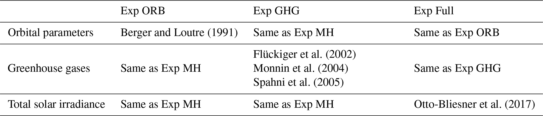
To enhance the rigor of our study and confirm the effects of ORBs and GHGs on the climate evolution from the MH to the PI, we conducted three additional transient experiments (Table 2). Each transient experiment starts at the MH and concludes at the PI, spanning a total of 5900 model years. Exp ORB represents the transient experiment for ORBs; Exp GHG is the transient experiment for GHGs; and Exp Full is the experiment where ORBs, GHGs, and total solar irradiance are applied concurrently. The ORB data in the transient experiments are from Berger and Loutre (1991), the GHG data are interpolated from GHG data reconstructed from Antarctic ice cores, and the total solar irradiance data are from the PMIP4 SATIRE-M solar forcing data (Otto-Bliesner et al., 2017). We use model years 1–500 to represent the MH climate (stage 1) and model years 5401–5900 to represent the PI climate (stage 2), and then compare the difference between stage 1 and stage 2 to the results of the equilibrium experiments (Fig. 5b). The settings for forcing information in the transient experiments are listed in Table 2.

Table 1 Forcings and boundary conditions in equilibrium experiments. More details can be found in Otto-Bliesner et al. (2017).

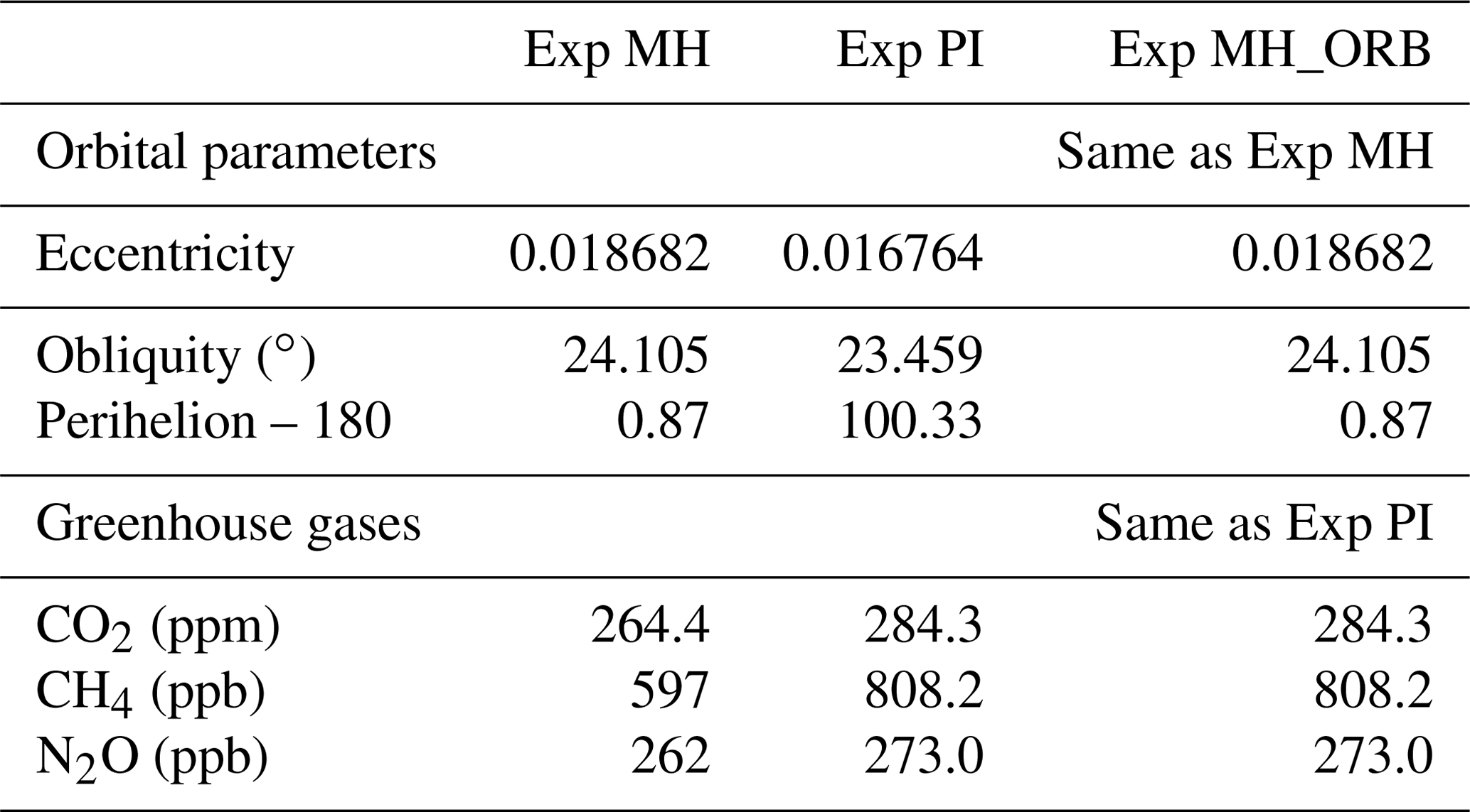
Table 2 Forcing and boundary conditions in transient experiments.

Orbital parameters include eccentricity, precession, and obliquity. In the past 6 Myr, both eccentricity and obliquity have not changed much. The main change came from precession, which is influenced by eccentricity and the longitude of perihelion. As a result, perihelion is close to the NH autumn equinox in the MH period and close to the NH winter solstice in the PI period. Therefore, with respect to Exp PI, the solar energy received at the top of the atmosphere (TOA) in Exp MH changed seasonally and latitudinally, as shown in Fig. 1a. Compared to Exp PI, Exp MH had higher NH summer radiation and lower winter radiation, and the difference during June–August (JJA) reached 30 W m⁻² in the high latitudes. Smaller precession led to more radiation received in the NH summer in the MH period. Figure 1b shows the meridional variation in the annual mean shortwave radiation at the TOA, which is greater than 4 W m⁻² poleward of 45^∘ N (S), but negative and smaller than 1 W m⁻² between 45^∘ S and 45^∘ N. This situation is associated with the larger obliquity in the MH (Otto-Bliesner et al., 2006; Williams et al., 2020). In addition, the difference in the GHGs between the MH and PI periods can lead to an effective radiative forcing of 0.3 W m⁻² (Otto-Bliesner et al., 2017).

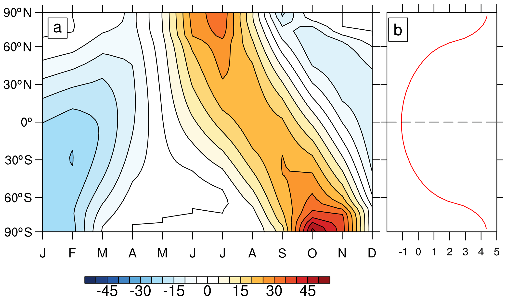
Figure 1 (a) Latitude–month distribution of solar radiation change at the TOA in Exp MH and (b) annual mean solar radiation change, with respect to Exp PI. The units are given in watts per meter squared (W m⁻²).

3 Results

3.1 Surface air temperature and precipitation

Compared to Exp PI, Exp MH has warmer annual mean temperatures in the NH high latitudes and cooler temperatures in the rest of the globe (Fig. 2a), while Exp MH_ORB has a warmer surface at mid–high latitudes in both the NH and SH, with a greater range and magnitude than Exp MH (Fig. 2b). Figure 2b shows the direct response to the meridional change in the annual mean solar radiation. The lower GHGs in the MH contributed to a lower global surface temperature, which is clear in the mid–high latitudes (Fig. 2c). In the NH summer (JJA), Exp MH shows a general warming of more than 1 ^∘C at 30^∘ N, which is more significant in Greenland and Eurasian continent, and a cooling belt in northern India and central Africa (Fig. 2d), which is associated with increased rainfall due to the enhanced monsoon (Fig. 2d). The magnitude and extent of warming due to the ORB effect are apparently greater, with warming of up to 3 ^∘C in central Asia (Fig. 2e). The GHG cooling is more pronounced over the Southern Ocean (Fig. 2f). In the NH winter (December–February or DJF), only the NH polar latitudes remain the warming. There is strong cooling (up to 3 ^∘C) in the African and Eurasian continents (Fig. 2g). The patterns under the ORB and GHG forcing are similar to their annual mean situations, except for the enhanced cooling in South Asia and central Africa (Fig. 2h) and over the subpolar Atlantic (Fig. 2i). Most figures show polar amplification, which may be related to the change in the sea ice (Otto-Bliesner et al., 2017; Williams et al., 2020).

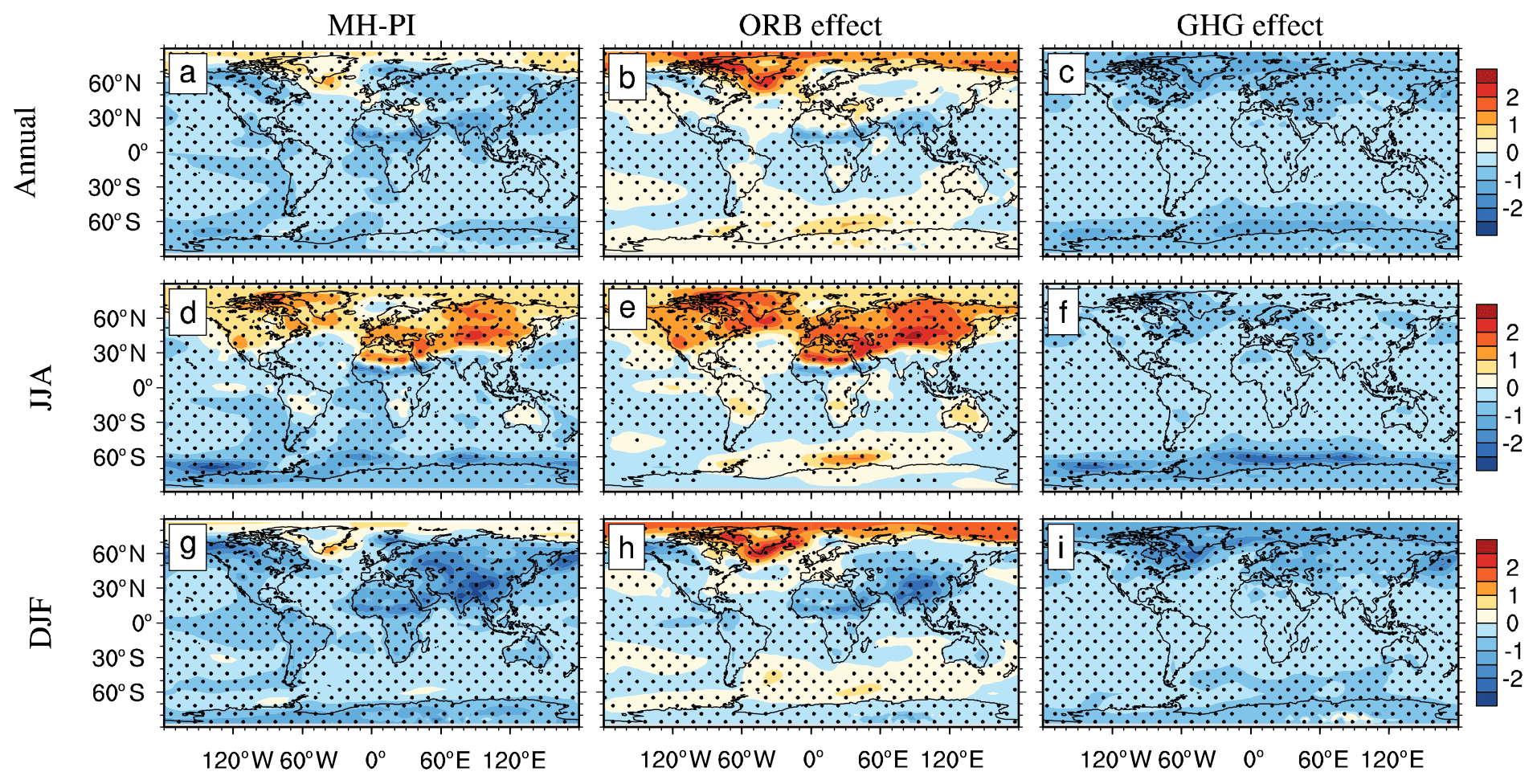
Figure 2 (a, d, g) Changes in SAT in Exp MH with respect to Exp PI and the contributions from (b, e, h) the ORB effect and (c, f, i) the GHG effect. Panels (a)–(c) show the annual mean. Panels (d)–(f) show the NH JJA. Panels (g)–(i) show the NH DJF. Stippling shows significance over the 90 % level calculated by Student t test. The units are given in degrees Celsius (^∘C).

Differences in precipitation between the MH and PI simulations are shown in Fig. 3. Consistent with the latitudinal and seasonal differences in the insolation (Fig. 1), the largest difference in precipitation between the two periods also occurs in the NH summer, with significantly more precipitation in the monsoon regions of northern India and equatorial African and drier conditions in the equatorial Atlantic and Pacific regions in Exp MH (Fig. 3d). The difference between Exps MH and PI is mainly in the global tropics and is contributed predominantly by the ORB effect (Figs. 3e, h), as the GHG effect is very weak (Figs. 3f, i).

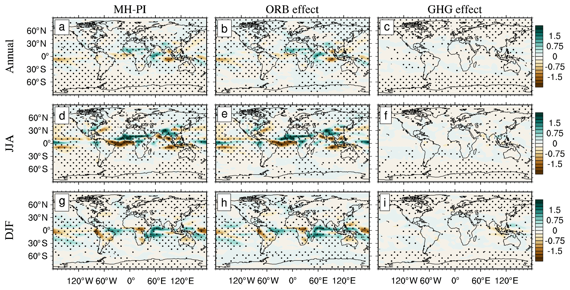
Figure 3 Same as Fig. 2 but for precipitation change. The units are given in millimeters per day (mm d⁻¹).

Although the numerical values may be slightly different due to different models or resolutions, in general the annual and seasonal climatology differences in the temperature and precipitation between Exps MH and PI are in good agreement, according to recent studies (Williams et al., 2020; Q. Zhang et al., 2021). The ORB effect dominates the changes in global surface temperature and precipitation. Thus, Exp MH has a warmer climate than Exp PI, particularly in NH high latitudes.

3.2 Meridional atmospheric circulation

The meridional atmospheric circulation, namely the Hadley cell, in Exp MH is about 10 % weaker than that in Exp PI (Fig. 4a), which is consistent with the weaker meridional atmospheric temperature gradient in Exp MH than in Exp PI. The weaker Hadley cell in Exp MH is mainly due to the ORB effect (Fig. 4b, e, h). The GHG effect can be neglected (Fig. 4c, f, i). The Hadley cell is weaker due to the strong warming of the high-latitude temperatures in the NH summer (Fig. 4d). The strengthening of the Hadley cell in the NH winter (Fig. 4g) corresponds to an increasing temperature gradient between the tropics and midlatitudes (Fig. 2g). The weaker Hadley cell also leads to a weaker meridional atmospheric heat transport from low to high latitudes, which will be discussed in Sect. 3.4.

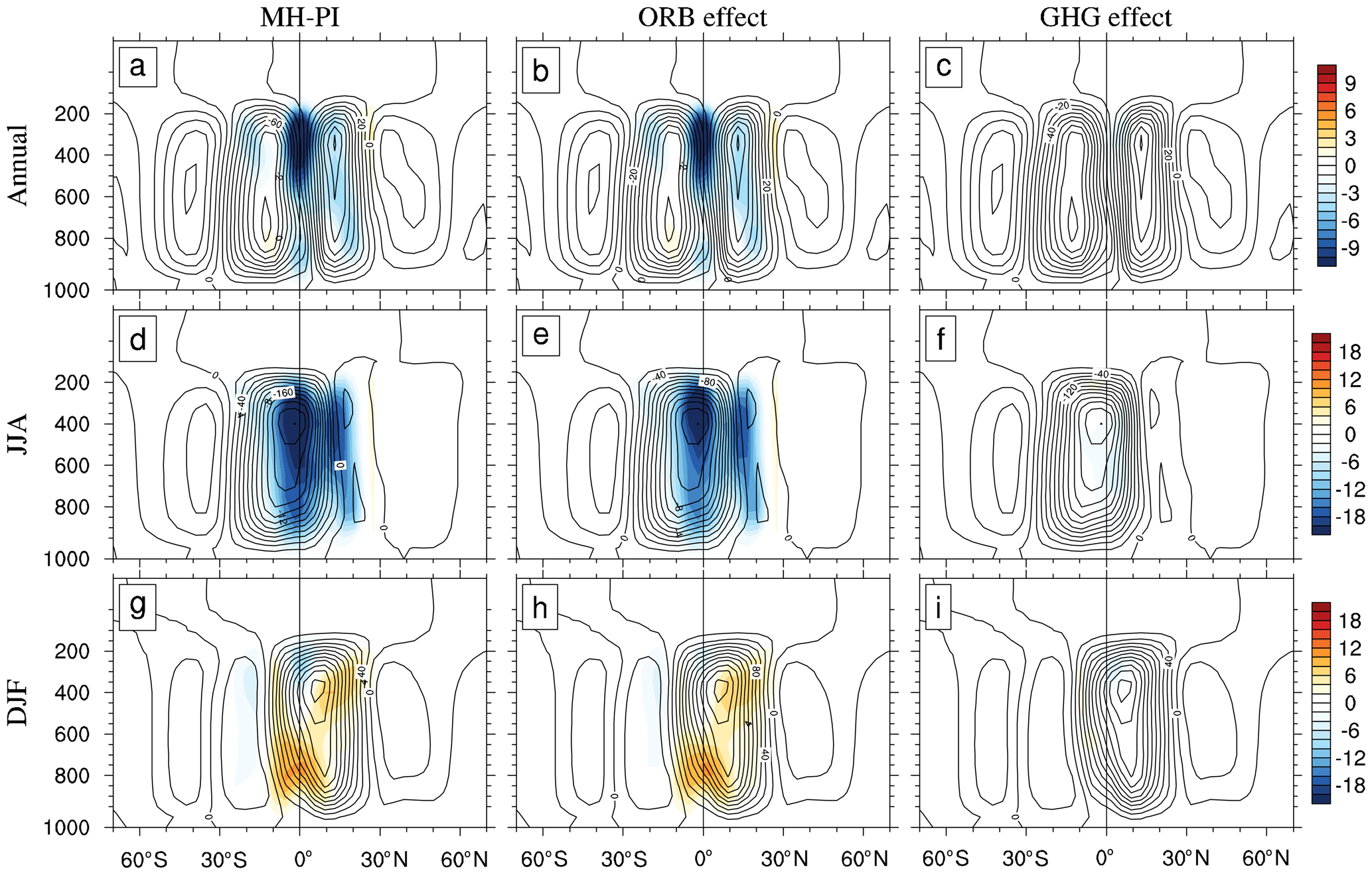
Figure 4 Same as Fig. 2 but for the mean Hadley cell in Exp PI (contour) and its changes (shading) in Exp MH. The units are 10⁹ kg s⁻¹.

3.3 Atlantic meridional overturning circulation

The AMOC strength, defined as the maximum streamfunction between 0 and 2000 m and between 20 and 70^∘ N in the North Atlantic, is 19.4 and 18.3 Sv in Exps MH and PI, respectively. Figure 5a shows the time series of the AMOC of the three equilibrium experiments, all of which reached the equilibrium state. The AMOC in Exp MH_ORB (dark blue line) is 1 Sv stronger than that in Exp PI (dark red line), while the AMOC in Exp MH (dark black line) is roughly the same as that in Exp MH_ORB. Figure 5b shows the evolution of the AMOC in the three transient experiments. In Exp ORB, the AMOC strength shows a downward trend (dark blue line). In Exp GHG, the AMOC strength exhibits a slight increase with an indistinct trend (dark red line). In Exp Full, the trend of AMOC strength is essentially between Exps ORB and GHG, indicating a combined effect of external forcing factors (dark black line).

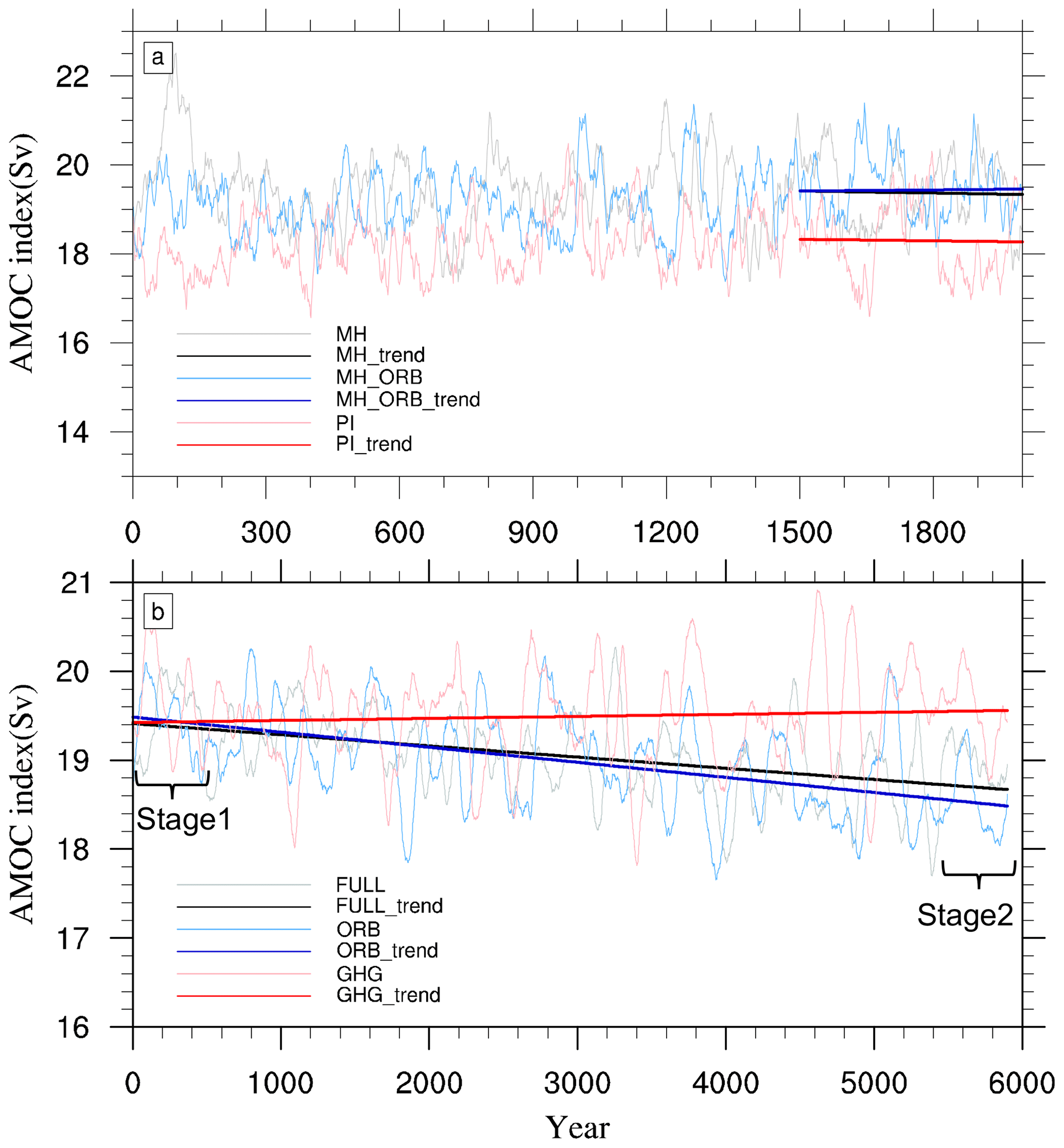
Figure 5 (a) Evolutions of the AMOC in Exp MH (gray and black lines), Exp MH_ORB (blue lines), and Exp PI (red lines). (b) Evolutions of the AMOC in Exp Full (gray and black lines), Exp ORB (blue lines), and Exp GHG (red lines). The thick lines indicate the linear trends of the AMOC in different experiments. The units are given in Sverdrups (1 Sv = 10⁶ m³ s⁻¹).

The patterns of the AMOC are shown in Fig. 6; the depth of the maximum AMOC in all experiments occurs near 1000 m. The AMOC patterns in Exps MH and PI are similar (Fig. 6a, c), which suggests that the combined effect of the ORBs and GHGs on the AMOC is small (Fig. 6d). This is similar to some recent studies, even though there are slight differences north of 45^∘ N (Brierley et al., 2020; Williams et al., 2020). Individual effects of the ORBs and GHGs are not negligible (Fig. 6e, f). In fact, the ORB effect leads to 6 % stronger AMOC in Exp MH than in Exp PI (Fig. 6e). The deep overturning is significantly enhanced south of 45^∘ N, but slightly weakened north of 45^∘ N. However, at the same time the GHG effect leads to a slight decline in AMOC strength in Exp MH, especially above 1500 m south of 45^∘ N (Fig. 6f). The ORBs and GHGs have opposite effects on the AMOC, which make the AMOC in Exp MH roughly the same as that in Exp PI. Figure 6g–i further shows the effects of different forcing factors on the AMOC patterns in the transient experiments, which are similar to the changes in the equilibrium experiments (Fig. 6d–f), although there are differences in intensity. The offset effect between ORBs and GHGs in the transient experiments is the same as that in the equilibrium experiments. Some scholars have suggested that the change in the AMOC in Exp MH may come from internal variability (Williams et al., 2020), but it is clear from our simulations that changes in response to external forcings are the main reason for the variations that occur in Exp MH.

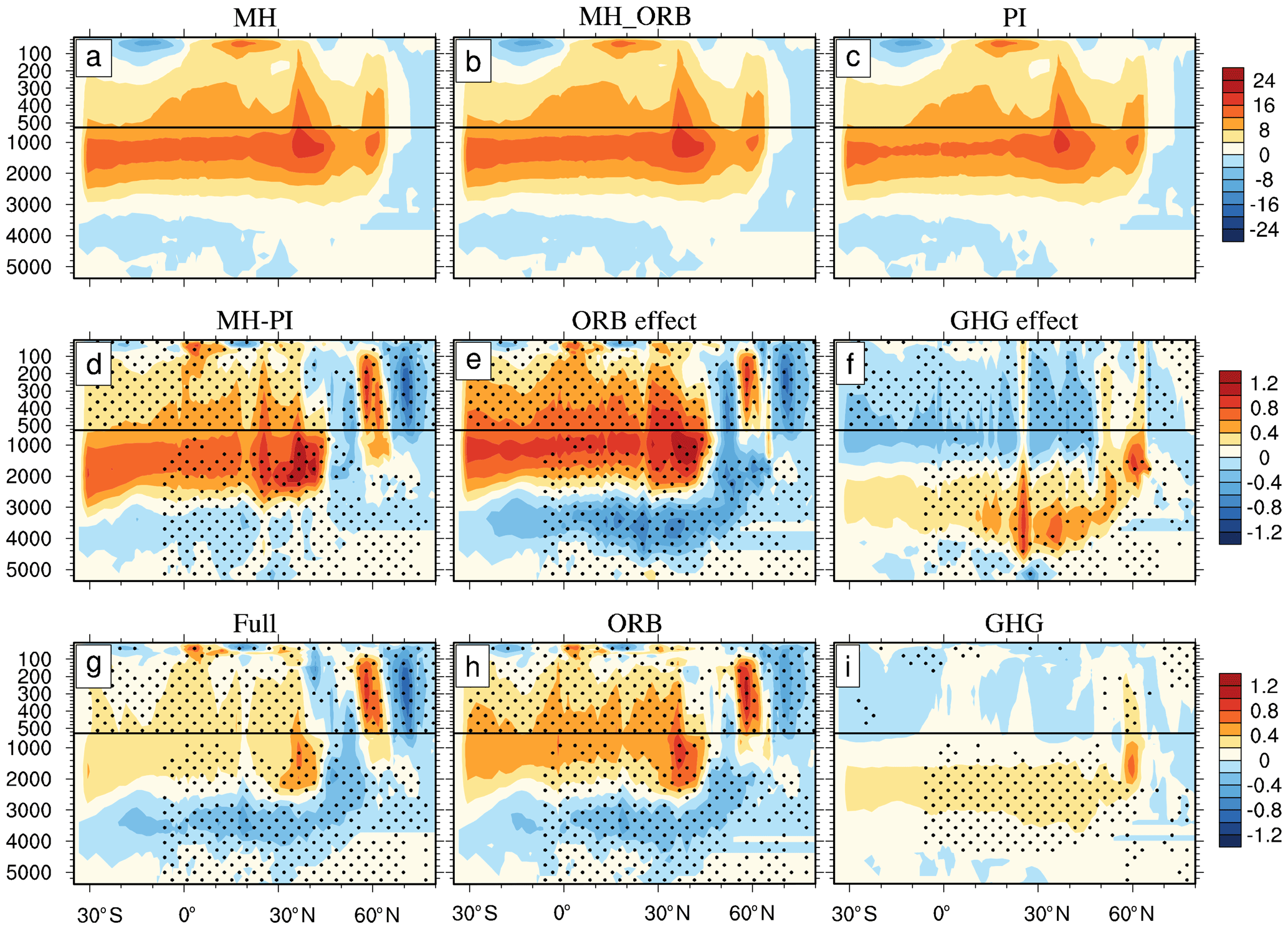
Figure 6 Patterns of mean AMOC in (a) Exp MH, (b) Exp MH_ORB, and (c) Exp PI. (d) The AMOC change in Exp MH, with respect to Exp PI. Panels (e) and (f) show AMOC changes due to the ORB effect and GHG effect, respectively. Panels (g), (h), and (i) represent the AMOC changes between the two stages (stage 1–stage 2) in Exps Full, ORB, and GHG, respectively. The AMOC index is defined as the maximum streamfunction in the range of 0–2000 m at 20–70^∘ N in the North Atlantic. Stippling shows significance over the 90 % level calculated by Student t test. The units are given in Sverdrups.

3.4 Meridional heat transport

Meridional heat transport (MHT) plays an important role in maintaining energy balance of the Earth's climate system. Figure 7a shows the annual MHT in different experiments, which are nearly identical. The climate differences between Exps MH and PI hardly change the integrated heat transport in both the atmosphere and ocean. Consistent with previous studies (Trenberth and Caron, 2001), the annual mean MHT shows an antisymmetric structure near the Equator, with the peak value of about 5.5 PW (1 PW = 10¹⁵ W) at 40^∘ N, 40^∘ S. Compared with ocean heat transport (OHT), the atmosphere heat transport (AHT) dominates at most latitudes, which is also consistent with previous studies (Held, 2001; Wunsch, 2005; Czaja and Marshall, 2006).

However, the MHT changes caused by the ORB and GHG effects appear to be nonnegligible. The ORBs cause an increase in OHT in the NH, with the maximum change of about 0.10 PW near the Equator, which is roughly 10 % of the mean OHT there. This is due to the enhanced AMOC and is the main cause of the temperature increase in the NH high latitudes (Fig. 2b). The northward AHT is reduced, with a maximum change of about 0.10 PW. This is due to the weakened Hadley cell. The AHT change compensates for the OHT change very well in the deep tropics, while the former overcompensates the latter in the NH off-equatorial regions (Fig. 7b). The GHG effect on the MHT is very weak, with a maximum MHT change of no more than 0.04 PW near 5^∘ N (Fig. 7c), which is just one-third of the ORB-induced MHT change (Fig. 7b).

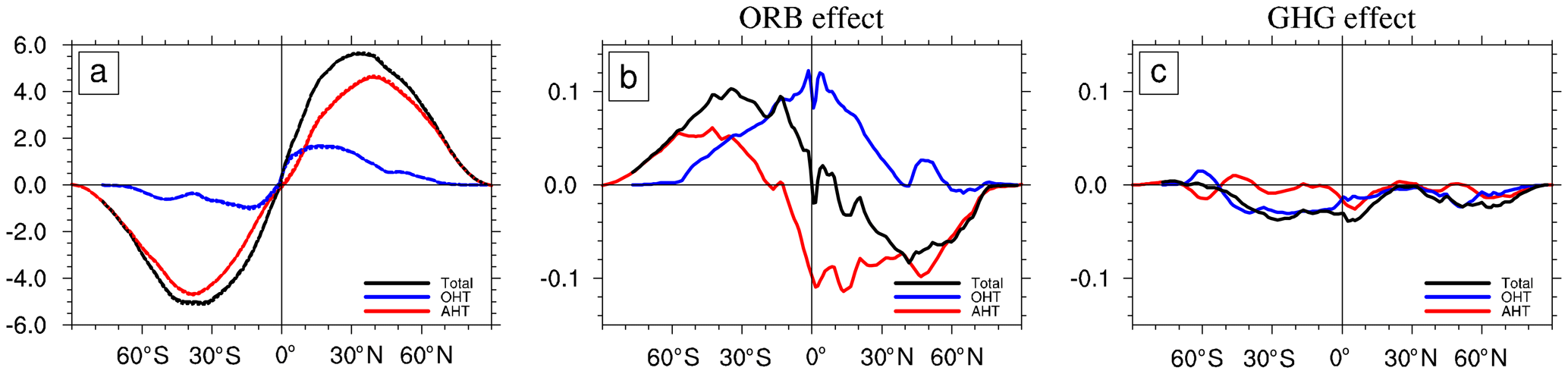
Figure 7 (a) Annual mean meridional heat transport (MHT). Black, red, and blue lines indicate the total MHT, AHT, and OHT, respectively. Solid, dashed, and dotted lines are for Exps MH, MH_ORB, and PI, respectively. Panels (b) and (c) show changes in the total MHT, AHT, and OHT due to ORB and GHG effects, respectively. The units are given in petawatts (1 PW = 10¹⁵ W).

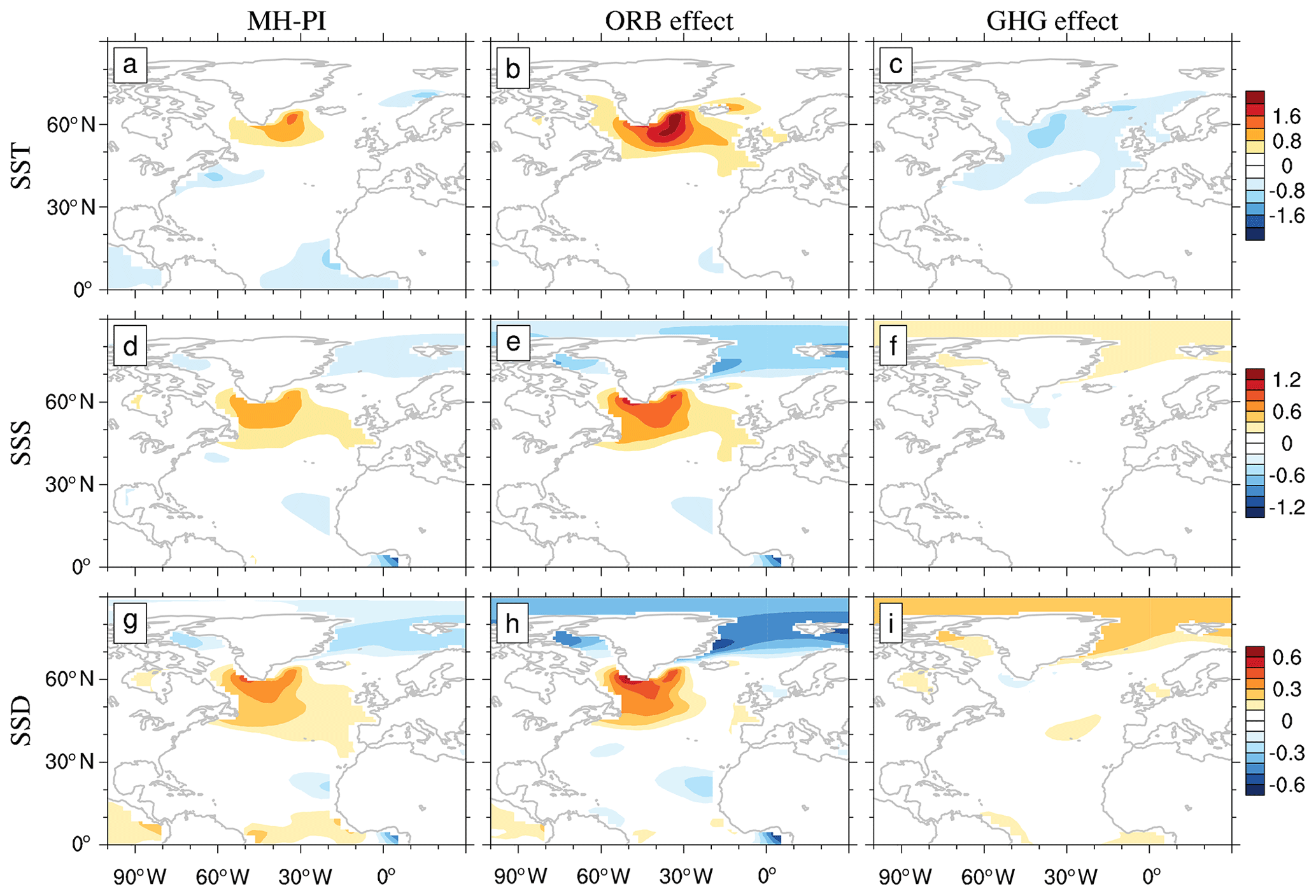
Figure 8 Changes in the (a)–(c) sea surface temperature (SST), (d)–(f) sea surface salinity (SSS), and (g)–(i) sea surface density (SSD) of the North Atlantic in Exp MH, with respect to Exp PI. Panels (a), (d), and (g) show the total changes. Panels (b), (e), and (h) show the changes due to the ORB effect. Panels (c), (f), and (i) show changes due to the GHG effect. The units are given in degrees Celsius (^∘C) for SST, practical salinity units (psu) for SSS, and kilograms per meter cubed (kg m⁻³) for SSD.

4 Changes in North Atlantic Ocean

4.1 Changes in sea surface temperature, salinity, and density

The strength of the AMOC is largely determined by the North Atlantic deepwater formation, which is in turn determined by upper-ocean density. Figures 8 and 9 show the differences in the sea surface temperature (SST), salinity (SSS), and density (SSD) in the North Atlantic between Exps MH and PI and the two stages in the transient experiments, respectively. The SST difference is characterized by a warming up to 1.6 ^∘C in the subpolar Atlantic and a cooling of about 1 ^∘C near the Nordic Seas and Gulf Stream extension region (Fig. 8a). The surface ocean warming in the North Atlantic is due to the ORB effect (Fig. 8b), which causes a strong and extensive warming in the North Atlantic, with the maximum warming in the subpolar Atlantic. This is in contrast to the warming hole shown by observations, which are dominated by the cooling of the North Atlantic in the context of global warming. The GHG effect causes a general cooling in the North Atlantic (Fig. 8c), partially offsetting the ORB-induced warming and leaving a cooling in the Nordic Seas and Gulf Stream extension (Fig. 8a). The North Atlantic SST change in Exp Full (Fig. 9a) is consistent with that of Exp MH (Fig. 8a), although the magnitude is slightly smaller. Exp ORB also exhibits stronger warming than Exp Full (Fig. 9b), consistent with Fig. 8b. Exp GHG shows a slight cooling (Fig. 9c), consistent with Fig. 8c. Overall, the SST change in the transient experiments is the same as that in the equilibrium experiments.

The patterns of the SSS difference between Exps MH and PI are similar to those of SST difference. In general, the North Atlantic is more saline in Exp MH than in Exp PI (Fig. 8d), mainly due to stronger evaporation over precipitation in Exp MH than in Exp PI (Fig. 12d), which is in turn due to the warmer SST forced by the ORB effect (Fig. 8e). The polar oceans are fresher in Exp MH than in Exp PI (Fig. 8d, e), mainly due to more freshwater flux coming from sea ice in Exp MH (Fig. 12a, b), consistent with the warmer climate in the MH due to the ORB effect. The SSS difference caused by the GHG effect is roughly opposite to that caused by the ORB effect, but with much weaker magnitude (Fig. 8f), because the cooling effect of the GHGs makes less evaporation in the subtropical–subpolar Atlantic and more sea ice in the polar oceans (Fig. 12c). Similar to the equilibrium experiments, the SSS changes in the transient experiments show similar characteristics (Fig. 9d, e, f).

The patterns of SSD difference (Fig. 8g–i) resemble those of both SSS and SST differences, while the polarity is determined by SSS difference. The higher SSD in the North Atlantic is favorable for a stronger deepwater formation and thus a stronger AMOC in Exp MH. Forced by the ORB effect, the North Atlantic surface ocean can be 0.5 kg m⁻³ denser in Exp MH than in Exp PI (Fig. 8h), which could have resulted in a 1.2 Sv stronger AMOC in Exp MH than in Exp PI (Fig. 6e). However, the GHG effect, although weak, has an opposite effect on SSD, and thus the AMOC (Fig. 8i), and eventually mitigates the ocean change in Exp MH. Similar patterns of SSD are shown in the transient experiments, with increased North Atlantic density in Exp ORB, and the opposite and weaker effect in Exp GHG (Fig. 9g, h, i), corresponding to changes in the AMOC (Fig. 6). These suggest that the mechanisms of ORBs and GHGs on climate change in the equilibrium and transient experiments are consistent.

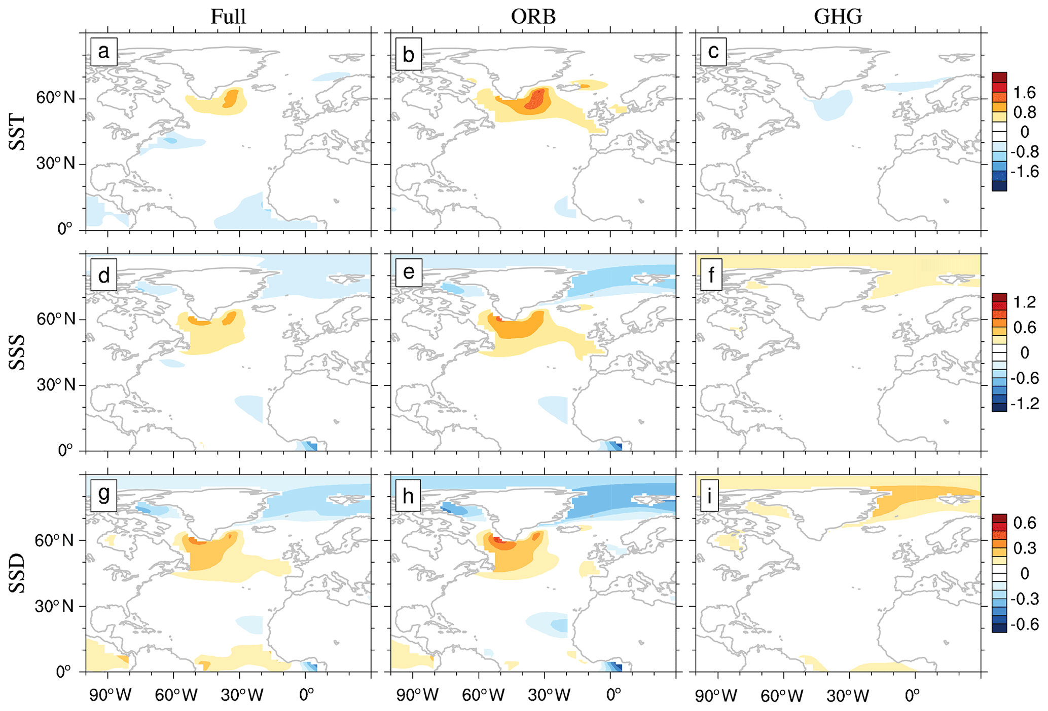
Figure 9 Similar to Fig. 8 but for Exps Full, ORB, and GHG, respectively. All variables represents changes between the two stages (stage 1–stage 2).

4.2 Change in surface freshwater flux

Sea surface freshwater flux includes both sea ice formation (melting) and net evaporation (i.e., evaporation minus precipitation or EMP). Figure 10 shows the change in the annual mean sea ice thickness in the Arctic. The Arctic sea ice thickness in Exp MH is about 1.0 m thinner than that in Exp PI (Fig. 10a). The largest sea ice difference, which is about 3.0 m thinner in Exp MH, occurs in Baffin Bay. When forced by the ORB effect only, the Arctic sea ice would be more than 1.5 m thinner (Fig. 10b), which is consistent with the stronger insolation and the warming in the NH high latitudes (Fig. 1, 2e). The GHG effect leads to a slight increase in the sea ice in the Arctic (Fig. 10c) in Exp MH, which is less than 0.5 m in thickness. Changes in Arctic sea ice thickness can affect sea ice transport to the subpolar Atlantic. The loss of sea ice in the central Arctic Ocean can reduce its export through the Fram Strait, which can lead to an increase in salinity in the associated subpolar regions (Shi and Lohmann, 2016), as shown in Fig. 8d and e. Similar changes in sea ice thickness also occur in the transient experiments because the Arctic sea ice thickness is decreased significantly in Exp ORB, while it is nearly unchanged in Exp GHG (Fig. 10e, f), thus reflecting the consistency of the effects of ORBs and GHGs in both equilibrium and transient experiments.

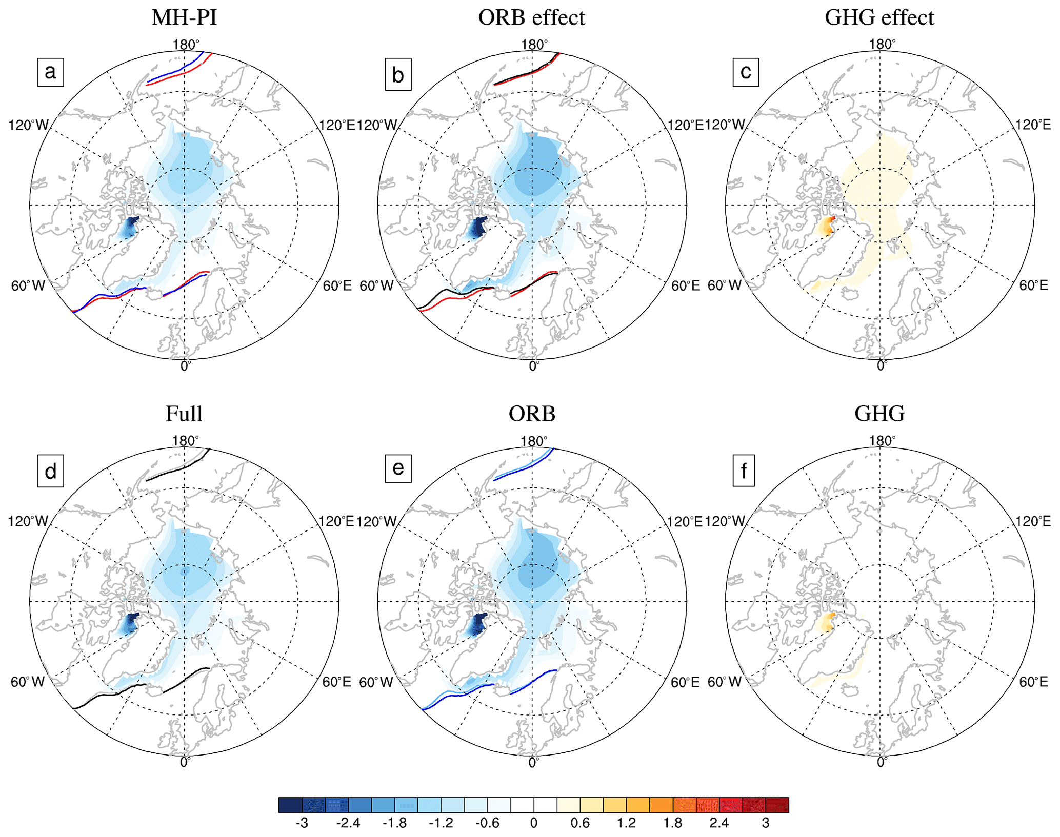
Figure 10 (a)–(c) Changes in Arctic mean sea ice thickness in Exp MH, with respect to Exp PI. The positive (negative) value represents sea ice formation (melting). Panel (a) shows the total change. Panels (b) and (c) show changes due to ORB and GHG effects, respectively. Solid blue, black, and red curves show the sea ice margin in Exps MH, MH_ORB, and PI, respectively. Panels (d)–(f) are the same as panels (a)–(c), except for Exps Full, ORB, and GHG, respectively. The solid gray and light blue curves indicate the sea ice margin of stage 1 in Exps Full and ORB, respectively. The solid black and dark blue curves represent the sea ice margin of stage 2 in Exps Full and ORB, respectively. The sea ice margin is defined by the 15 % sea ice fraction. The units are in meters.

The sea ice margin in the North Atlantic in Exp MH is slightly more northward compared to that in Exp PI (solid blue curve; Fig. 11a). The curves in Fig. 11 show sea ice margin in different experiments. The northward displacement of the sea ice margin and the decrease in sea ice volume in the Arctic favor the decrease in freshwater flux in the North Atlantic, helping a more saline North Atlantic, which contributes about 0.9 psu per decade to the SSS tendency between 40 and 60^∘ N (Fig. 11a). The EMP flux is small, and the upper ocean is refreshed at a steady rate of about 0.09 psu per decade in the North Atlantic (Fig. 11d). The contributions of sea ice change and EMP flux to SSS in the transient experiments are also about 0.9 and 0.09 psu per decade, respectively (Fig. 11g, j). Overall, for the North Atlantic, the change in the sea ice plays a dominant role, and its contribution to SSS tendency is about 10 times that of EMP.

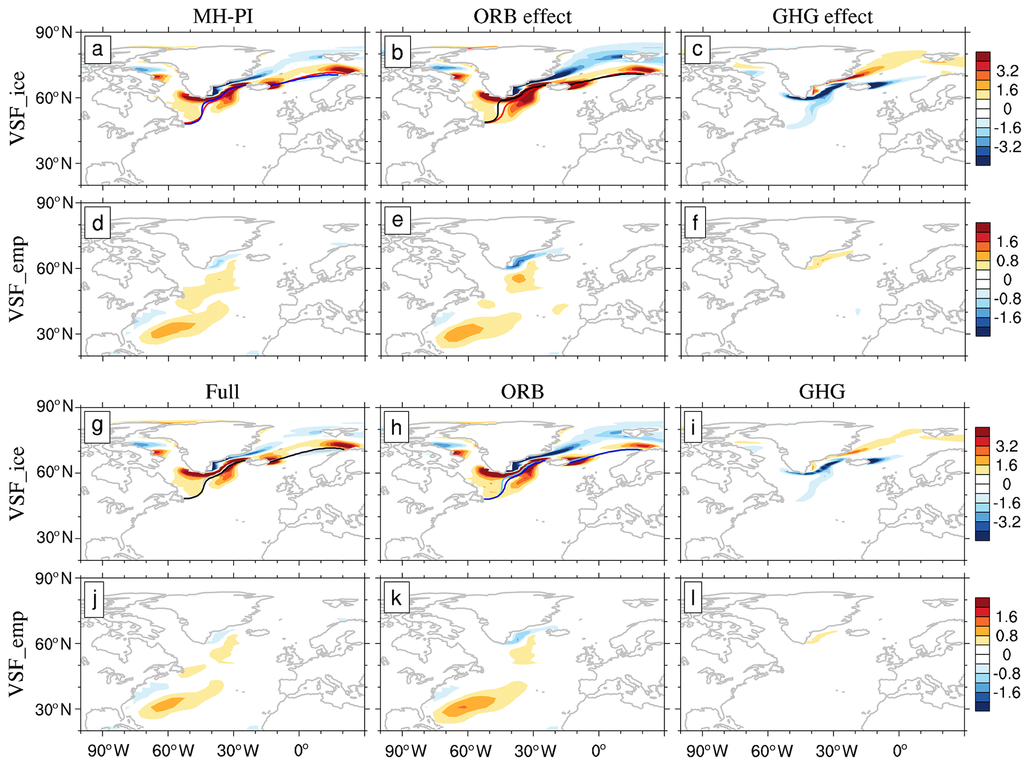
Figure 11 Changes in panels (a)–(c), with virtual salt flux (VSF) due to sea ice, and in panels (d)–(f), with VSF due to EMP in Exp MH (with respect to Exp PI). The positive (negative) value represents sea ice formation (melting) or evaporation that is larger (smaller) than precipitation. Panels (a) and (d) show the total changes. Panels (b) and (e) show the changes due to the ORB effect. Panels (c) and (f) show the GHG effect. Panels (g)–(l) are the same as panels (a)–(f) but for Exp Full, Exp ORB, and Exp GHG, respectively. The solid gray and light blue curves indicate the sea ice margin of stage 1 in Exps Full and ORB, respectively. The solid black and dark blue curves represent the sea ice margin of stage 2 in Exps Full and ORB, respectively. The sea ice margin in panels (a)–(b) is defined the same way as that in Fig. 8. The units are given in practical salinity units per decade.

The sea ice margin in Exp MH is controlled by the ORB effect. In the individual forcing experiment, the sea ice margin forced by the ORB effect is almost the same as that in Exp MH (solid black curve; Fig. 11b). The contributions of the ORB and GHG effects to changes in virtual salt flux (VSF) due to sea ice are 1.3 and −0.4 psu per decade, respectively (Fig. 11b, c), and those due to the EMP flux are 0.06 and 0.03 psu per decade, respectively (Fig. 11e, f). In the transient experiments, the contributions of ORB and GHG effects to the VSF due to sea ice are 1.1 and −0.2 psu per decade, respectively (Fig. 11h, i), and those due to EMP flux are 0.05 and 0.03 psu per decade, respectively (Fig. 11i, l). This suggests that the sea ice change caused by the ORB effect plays an important role in the enhancement of the AMOC in Exp MH.

In general, the modeling results suggest that the stronger AMOC in the MH period resulted from more saline North Atlantic, which was contributed mainly by smaller freshwater flux coming from the Arctic. The contribution of EMP to salinity change was small, which was only $\mathrm{1}/\mathrm{10}$ of the sea ice contribution. ORBs and GHGs consistently play opposite roles in the deepwater formation of the subpolar Atlantic. Their combined effect resulted in little change in the AMOC in the MH period, which is less than 1 Sv enhancement in both equilibrium and transient experiments.

5 Summary and discussion

In this study, six experiments using the CESM1.0 were conducted to quantify the contributions of ORB and GHG effects to the MH climate. Most of our attention was paid to the AMOC, and the mechanism of the insignificant difference in the AMOC between the MH and PI periods was explored. This study is the first attempt to separate the ORB and GHG effects on the MH climate. Simulations showed that the NH climate exhibits much greater regional and seasonal variability due to the seasonal enhancement of insolation caused by changes in ORBs, and these contrasting seasonal responses lead to little change in the annual mean climate. Lower GHGs in Exp MH have a global cooling effect, with greater temperature decreases at higher latitudes associated with feedbacks from sea ice and snow cover. The combined effect of these two forcing factors leads to a weak warming at the NH high latitudes and cooling elsewhere, which is similar to the temperature changes in the PMIP4 ensemble (Brierley et al., 2020).

The weakening meridional atmospheric temperature gradient in Exp MH leads to the Hadley cell being weakened by about 10 % in the NH. At the same time, due to the change in the sea surface buoyancy in the North Atlantic, the AMOC is slightly enhanced by about 4 %. As far as the changes in MHT magnitude in the NH are concerned, the effect of ORBs is about 5 times that of GHGs. Our experiments also showed that the change in the AMOC is mostly determined by the freshwater flux change in the North Atlantic, which is in turn closely related to the Arctic sea ice change related to the ORB effect. GHGs have the opposite effect to ORBs, which mitigates the enhancement of the AMOC (Fig. 9b, c).

The conclusions drawn in this paper may be dependent on the model. Shi and Lohmann (2016) simulated a stronger MH AMOC in the high-resolution version of the ECHAM, with a maximum change of more than 2 Sv. Most of the models in the CMIP5 reveal a positive AMOC change in the MH period. Some previous studies (Ganopolski et al., 1998; Otto-Bliesner et al., 2006) showed that the AMOC in the MH is weaker than that of the PI period. The main reason for the inconsistency is that the simulated ocean salinity in the North Atlantic is different. Therefore, it is necessary to carry out simulations with multiple models to reduce model dependence. Our simulations of the AMOC in the MH are similar to those of Jiang et al. (2023a), both showing no significant changes in the AMOC in the MH compared with the PI; however, their study did not explain the mechanism behind this phenomenon. Our study reveals the competitive relationship between the two forcing factors through multiple-equilibrium state simulations and transient simulations, supporting the popular conclusions about the AMOC change from the MH to the PI periods.

Our study focuses on the effects of ORB and GHG, and the simulated cooler annual mean temperature in most areas of the NH differs from the warming record revealed by most proxy data (Wanner et al., 2008; Liu et al., 2014) but is similar to the conclusions from the PMIP4 simulations. It is unclear whether these differences originate from the model, the data record, or a combination of the two. Some proxy data suggested that the climate of northern Africa was wetter in the MH period, which was known as the green Sahara (Larrasoaña, 2012). Jiang et al. (2012) analyzed the simulation results of six coupled models in PMIP2 for the MH period. They found that the dynamic vegetation effect led to a decrease in annual cooling over China in five of these models during the MH period, although its impact on the MH temperature was minimal. Braconnot et al. (2021) and M. Zhang et al. (2021) studied the effect of dust reduction on climate due to the greening of the Sahara desert, using the CESM and IPSL models, respectively, showing global mean surface temperature increased by about 0.1 ^∘C. Although there are other forcing factors in the MH period, such as vegetation, dust, and topography, overall, our simulations are representative of the most important forcing factors and provide quantified estimates of the contributions of ORB and GHG effects on the MH climate.