Synchronizing ice-core and U ∕ Th timescales in the Last Glacial Maximum using Hulu Cave ¹⁴C and new ¹⁰Be measurements from Greenland and Antarctica

Between 15 and 27 kyr b2k (thousands of years before 2000 CE) during the last glacial, Greenland experienced a prolonged cold stadial phase, interrupted by two short-lived warm interstadials. Greenland ice-core calcium data show two periods, preceding the interstadials, of anomalously high atmospheric dust loading, the origin of which is not well understood. At approximately the same time as the Greenland dust peaks, the Chinese Hulu Cave speleothems exhibit a climatic signal suggested to be a response to Heinrich Event 2, a period of enhanced ice-rafted debris deposition in the North Atlantic. In the climatic signal of Antarctic ice cores, moreover, a relative warming occurs between 23 and 24.5 kyr b2k that is generally interpreted as a counterpart to a cool climate phase in the Northern Hemisphere. Proposed centennial-scale offsets between the polar ice-core timescales and the speleothem timescale hamper the precise reconstruction of the global sequence of these climatic events. Here, we examine two new ¹⁰Be datasets from Greenland and Antarctic ice cores to test the agreement between different timescales, by taking advantage of the globally synchronous cosmogenic radionuclide production rates.

Evidence of an event similar to the Maunder Solar Minimum is found in the new ¹⁰Be datasets, supported by lower-resolution radionuclide data from Greenland and ¹⁴C in the Hulu Cave speleothem, representing a good synchronization candidate at around 22 kyr b2k. By matching the respective ¹⁰Be data, we determine the offset between the Greenland ice-core chronology, GICC05, and the Antarctic chronology for the West Antarctic Ice Sheet Divide ice core (WDC), WD2014, to be 125 ± 40 years. Furthermore, via radionuclide wiggle-matching, we determine the offset between the Hulu speleothem and ice-core timescales to be 375 years for GICC05 (75–625 years at 68 % confidence) and 225 years for WD2014 (−25–425 years at 68 % confidence). The rather wide uncertainties are intrinsic to the wiggle-matching algorithm and the limitations set by data resolution. The undercounting of annual layers in GICC05 inferred from the offset is hypothesized to have been caused by a combination of underdetected annual layers, especially during periods with low winter precipitation, and misinterpreted unusual patterns in the annual signal during the extremely cold period often referred to as Heinrich Stadial 1.

1 Introduction

Well-dated paleoclimatic archives, such as ice cores or speleothems, are essential for reconstructing the mechanisms of past climate change. Independent chronologies for each climatic archive are necessary for studying the recorded signals and are determined via, for example, counting annual layers or based on U $/$ Th measurements. However, the uncertainties in each timescale and a lack of matching horizons hamper the global comparison of climatic proxy records.

During the Last Glacial Maximum (LGM) the ice sheets were at their largest extent (defined as ca. 23.3–27.5 ka by Hughes and Gibbard, 2015, although other definitions exist), and extreme climatic shifts were recorded in the Greenland and Antarctic ice cores, as well as in Asian speleothems such as the ones from Hulu Cave, China (Wang et al., 2001). To advance our knowledge of the LGM as recorded in the archives, we need to estimate the leads and lags between these shifts, but a climatic synchronization is not always possible and not free of interpretation caveats. A lack of secure tie points over the LGM by most synchronization studies (Svensson et al., 2020; Corrick et al., 2020; WAIS project members, 2015) makes the reconstruction of a global sequence of events difficult to assess.

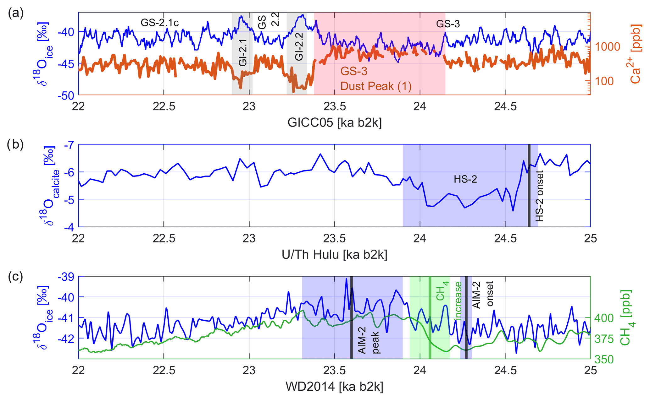
Figure 1 Climate signals on their original timescales. The time direction is from right to left. The references to all datasets are summarized in Table 1. Notice the relative position of onsets and terminations of the climate shifts. (a) Greenland stable oxygen isotopes (GRIP) and calcium (log scale, NorthGRIP), showing the alternating signals of interstadials (GIs) and stadials (GSs), as defined by Rasmussen et al. (2014), and the dust peak during GS-3. (b) Hulu Cave stable oxygen isotopes, on a reversed y axis, showing the cold phase attributed to HS-2. (c) Antarctic (WDC) stable oxygen isotopes showing the Antarctic Isotope Maximum 2 (AIM-2; EPICA community members, 2006) and the methane record showing a rapid increase.

In Greenland ice cores, the water stable isotope data (e.g. δ¹⁸O_ice) record two unusually short and small Greenland interstadials, GI-2.1 and GI-2.2 (Rasmussen et al., 2014), briefly interrupting the long cold period formed by the two Greenland stadials GS-2 and GS-3 (Fig. 1a). Despite other periods of interstadial climate conditions being recorded widely across the Northern Hemisphere, there is no counterpart of the brief GI-2.1 and GI-2.2 in the Hulu δ¹⁸O_calcite (Fig. 1b), which hampers the comparison of Greenland ice cores and Asian speleothems.

Around the same time, the δ¹⁸O_ice in several Antarctic ice cores reaches a maximum (AIM-2; EPICA Community Members, 2006), interrupting a warming trend (Fig. 1c). Greenland and Antarctic δ¹⁸O_ice records are hypothesized to be coupled by the bipolar seesaw mechanism (Stocker and Johnsen, 2003), by which a Greenlandic transition to an interstadial will initiate cooling in Antarctica with a small delay. According to the current chronologies, however, the onset of the Antarctic cooling, i.e. the peak of the AIM-2, leads the onset of the GI-2.2 by about 260 years. The average delay, or signal transmission time, from the North Atlantic to Antarctica is estimated to be 1 to 2 centuries, as shown by ice-core measurements (Svensson et al., 2020; WAIS project members, 2015) and in line with modelling experiments (Pedro et al., 2018), but the lead-lag dynamic appears to be reversed for AIM-2.

During GS-2 and GS-3, at least two massive discharge events of icebergs from the Laurentide Ice Sheet were inferred from the ice-rafted debris content of North Atlantic marine sediments, defining the occurrence of the Heinrich Events 1 and 2 (HE-1 and HE-2; Bard et al., 2000; Peck et al., 2006), which are now each thought to consist of 2 pulses. Heinrich events occurred during Greenland stadials and added a large amount of fresh water to the surface ocean, likely causing an extreme shutdown of the Atlantic Overturning Meridional Circulation (AMOC) and, thereby, prolonged climatic conditions of severe cold (McManus et al., 2004). The term Heinrich Stadial (HS) is often used to indicate the period affected by the Heinrich events.

Signatures of climatic change likely related to HS-1 and HS-2 are recorded in the δ¹⁸O_calcite of the Hulu speleothems (Fig. 1b; Cheng et al., 2018), but no counterpart is found in the Greenland δ¹⁸O_ice. Possible reasons include the high-latitude areas around the ice sheet not being strongly affected by the cooling or the isotopes reacting non-linearly (Guillevic et al., 2014). It has also been suggested that, during HS-1, changes in the precipitation seasonality influenced the annual mean δ¹⁸O_ice in a way that obscured the relation of δ¹⁸O_ice and annual average temperatures (He et al., 2021). This may also apply to HS-2. While δ¹⁸O_ice does not show a clear imprint of the Heinrich events, Greenland ice-core calcium data show two periods of heightened concentration during GS-3 (Fig. 1a; Rasmussen et al., 2014) that could be related to atmospheric reorganization around HE-2 (Adolphi et al., 2018), although there is debate about this attribution (Hughes and Gibbard, 2015). Since mineral dust aerosols in Greenland originate mostly from the Eurasian continent (Schüpbach et al., 2018), and the dust record therefore should reflect climate variability in Asia, Dong et al. (2022) synchronized the youngest Greenland calcium peak to the HS-2 signal of an Asian speleothem (Cherrapunji, India). Based on the assumption of synchronous climate signals, they inferred a multi-centennial dating offset between the Greenland ice-core chronology, GICC05, and the U $/$ Th-dated speleothem record that is consistent with earlier estimates based on cosmogenic radionuclides (Adolphi et al., 2018).

In addition to the Antarctic warming indicated by AIM-2, an abrupt rise in methane levels (Fig. 1c) indicates a likely response of the tropical methane emission sources to a period of climate change (Rhodes et al., 2015), which is suggested to correspond to HS-2. The phasing of the methane signal and the Heinrich Stadial 2 is still unresolved because of possible offsets in the respective chronologies.

The unclear causal relationships between the mentioned signals challenge the interpretation of the climate dynamics of the LGM. The timescale uncertainties in each archive, on the order of centuries for the ice-core chronologies (Svensson et al., 2008; Sigl et al., 2016), mask any absolute inference of the climatic leads and lags. Non-climatic synchronization horizons such as volcanic eruptions or solar events are needed to obtain solid estimates of the relative timescale offsets. For example, Svensson et al. (2020) compared the two layer-counted polar chronologies GICC05 (Greenland ice-core chronology; Svensson et al., 2008) and WD2014 (chronology of West Antarctic Ice Sheet Divide ice core, WDC; Sigl et al., 2016) via bipolar volcanic tie points. They found a negligible offset at 16 ka and only 80 years at 24.6 ka. However, they lack tie points within this entire interval.

Traces of cosmogenic radionuclides (e.g. ¹⁴C and ¹⁰Be) allow for global synchronizations because of their common production history and widely recorded signals. So far, the only radionuclide-based tie point in the LGM between ice-core and Hulu Cave records was found by Adolphi et al. (2018). Around 22 ka, they measured an offset of 550 years (95 % probability interval: 215–670 years) between GICC05 and the Hulu timescale, the latter being oldest.

This offset is unexpected considering the good agreement between the two chronologies measured both before and after the LGM; the climate synchronization between speleothems and GICC05 by Corrick et al. (2020) found small offsets of 4 years at GI-1 (15 ka) and of 92 years at GI-3 (27.5 ka). Nonetheless, the climatic synchronization by Dong et al. (2022) suggests that GICC05 is too young compared to the Cherrapunji speleothem U $/$ Th ages and estimates the offset to be 320 years (with a 2σ uncertainty of 90 years) around 24.5 ka. In addition, the WD2014 and Hulu timescales are offset by 167 years around GI-3 (Sigl et al., 2016), suggesting that the Antarctic ice-core chronology may also be diverging from U $/$ Th ages.

In this study, to better determine the sequence of events during the LGM, we aim at establishing strong ties between the three chronologies: GICC05 and WD2014, both dated by annual-layer counting, and Hulu Cave, dated by U $/$ Th measurements. Since the WD2014 chronology in the LGM was never compared against the Hulu and GICC05 chronologies, new Antarctic ¹⁰Be measurements are needed to fill the gap. Further, new ¹⁰Be measurements from Greenland are needed to strengthen the statistical significance of the 22 ka tie point by Adolphi et al. (2018), which presents a low signal-to-noise ratio. The Hulu Cave ¹⁴C_calcite and δ¹⁸O_calcite measurements were updated in recent years (Cheng et al., 2018) and directly included in the radiocarbon calibration curve (IntCal20; Reimer et al., 2020), used to date radiocarbon from organic samples worldwide. We therefore aim to evaluate the tie point by Adolphi et al. (2018) using new measurements of ¹⁰Be and the recent ¹⁴C_calcite. We use a combination of carbon-cycle modelling and statistical wiggle-matching (Siegenthaler, 1983; Adolphi and Muscheler, 2016) to directly compare proxy records from both polar ice sheets and the Hulu Cave.

In this work, we confirm the existence of centennial offsets in the LGM between the three chronologies, and we position the mentioned global climatic shifts in relation to each other. The question of why chronological offsets quickly develop remains open, but we suggest that difficulties with annual-layer identification in the very cold parts of the last glacial are the likely source of the observed offsets.

2 Data and methods

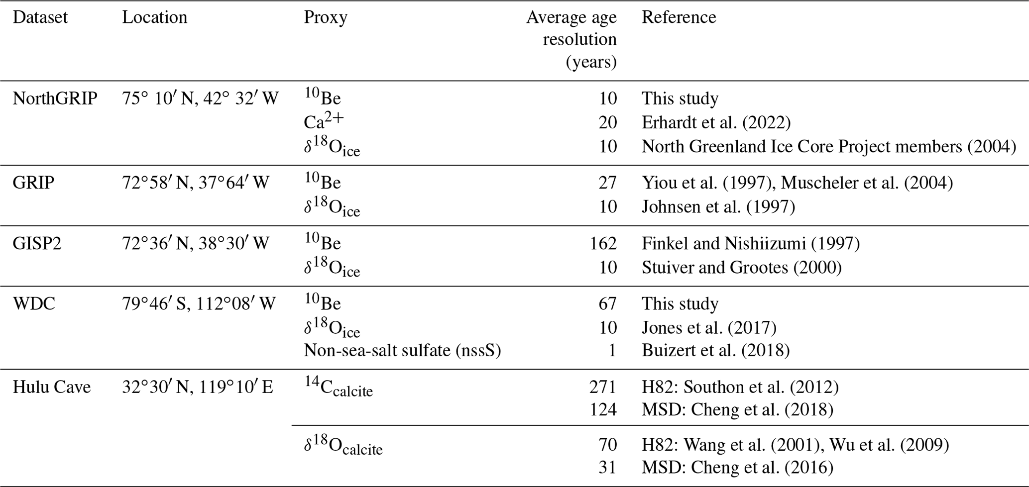
In this study, we aim at comparing the new cosmogenic radionuclide data with other datasets from Greenland, Hulu Cave, and Antarctica. We also analyse water stable isotope, methane, and calcium data to assess climatic changes. We summarize the relevant datasets, age resolutions, and citations in Table 1. In this work, we refer to years b2k (years before 2000 CE) because they are commonly used for the GICC05 timescale; when necessary, we have converted from years BP (before 1950 CE) by adding 50 years.

Table 1 Datasets used in this study. Age resolutions represent the period 20 to 25 kyr b2k. For the Hulu Cave, ¹⁴C_calcite data from two speleothems from the cave, labelled H82 and MSD, were published in two separate studies.

2.1 Preparation and measurement of the NorthGRIP samples

The 322 new Greenland ¹⁰Be measurements were performed at ETH Zurich on samples from the NorthGRIP ice core between 1726.45 and 1816.51 m depth, which according to GICC05 correspond to ages between 20 039 and 24 774 years b2k (Andersen et al., 2006). The samples have a variable temporal resolution between 7.5 and 14 years with some smaller gaps (see Appendix, Sect. A2) and are so far the best-resolved available radionuclide dataset for the LGM. The extraction of ¹⁰Be followed protocols by Nguyen et al. (2021); see Appendix, Sect. A3. The measured ¹⁰Be concentrations are shown in Fig. 2a.

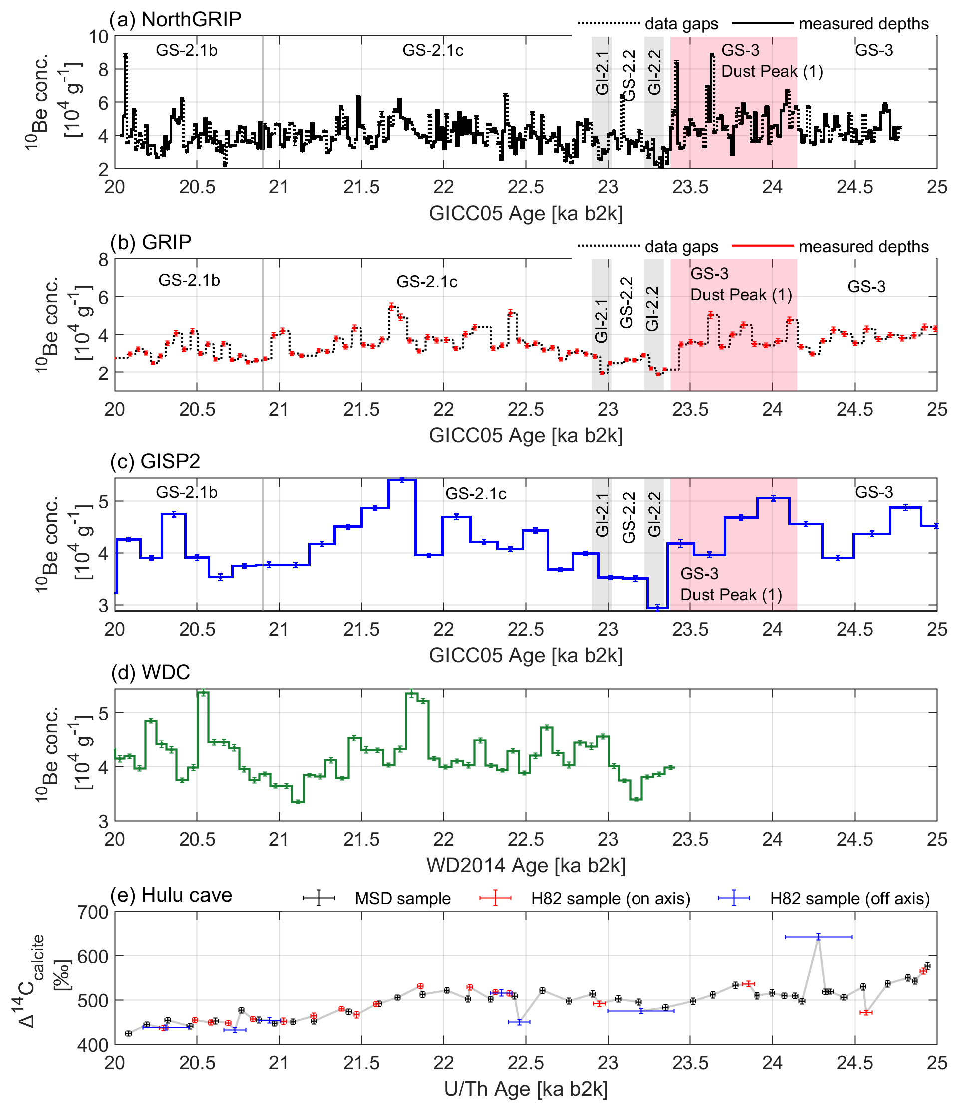
Figure 2 Cosmogenic radionuclide data used in this study (see Table 1 for references). On the GICC05 timescale: ¹⁰Be concentrations in (a) NorthGRIP, (b) GRIP, and (c) GISP2. Dotted lines in the GRIP data indicate discontinuities between every 55 cm resolved sample. On the WD2014 timescale: (d) WDC ¹⁰Be concentrations. On a U $/$ Th-based timescale: (e) Hulu Cave Δ¹⁴C_calcite data as reported in three separate datasets. In the following, we exclude the off-axis H82 measurements (blue), as they show more outliers and wider dating uncertainties.

2.2 Preparation of the WDC samples and measurement

A total of 73 samples in the West Antarctic ice sheet (WAIS) Divide 06A ice core (WDC-06A), from 2453 to 2599 m depth, were analysed for ¹⁰Be concentrations at Purdue University. These samples represent continuous ice-core sections with a cross-section of ∼ 2 cm², varying from 1.89 to 2.12 m in length (∼ 60–75 years of snow accumulation per sample). The extraction followed established protocols (Woodruff et al., 2013); see Sect. A1 for more details. Figure 2d shows the measured WDC ¹⁰Be concentrations.

2.3 Conversion of ¹⁰Be concentrations to fluxes

To account for the first-order correction of climatic influences on the ¹⁰Be signal (Adolphi et al., 2018), we need to convert the ¹⁰Be concentrations to fluxes, which requires knowledge of accumulation rates (see Sect. A3). Accumulation rates for the ice cores are reconstructed using the annual-layer thicknesses and an appropriate model for the layer thinning. The thinning in the LGM portion of the ice cores can be approximated by a linear function of depth, although there may be uncertainties that relate to the timescale itself.

For the NorthGRIP ice core, the layer thickness was directly derived from the annual layers of the GICC05 (Andersen et al., 2006), while the thinning was modelled by Johnsen et al. (2001). For WDC, the accumulation rate (Fudge et al., 2016) was inferred from the WD2014 layer thicknesses and modelled thinning (Buizert et al., 2015). The new ¹⁰Be fluxes are shown in Fig. 2, together with the modelled accumulation rates. The fluxes of NorthGRIP are clearly less affected by changing snow accumulation rates than ¹⁰Be concentrations, as seen in the absence of GI-/GS-related changes in ¹⁰Be, which is like other Greenland ice-core ¹⁰Be records (e.g. Muscheler et al., 2004). To show that the flux conversion largely removes the climatic influence on ¹⁰Be deposition in Greenland, we checked the residual correlations with other climate proxies in Fig. S3 in the Supplement.

Over the LGM, the GRIP and GISP2 ice cores were tied to NorthGRIP by identification of volcanic tie points and biomass burning events, and GICC05 was extended to these ice cores by interpolation (Rasmussen et al., 2008; Seierstad et al., 2014). The annual-layer thickness is thus less certain for GRIP and GISP2 and, due to a scarcity of volcanic tie points across the LGM, the accumulation difference across the short interstadials GI-2.1 and GI-2.2 may be at risk of misinterpretation. We used the most recent versions of GRIP and GISP2 thinning functions to calculate fluxes (Lin et al., 2022; Hvidberg et al., 1997), but we actively modified the accumulation history using new ¹⁰Be tie points, as delineated in Sect. 3.2. The ¹⁰Be measurements recently performed in the LGM on the NEEM ice core (Zheng et al., 2021) have similar resolution to the GISP2 dataset. The NEEM dataset does not resolve the ¹⁰Be features we are studying well, and we therefore do not consider this dataset further on.

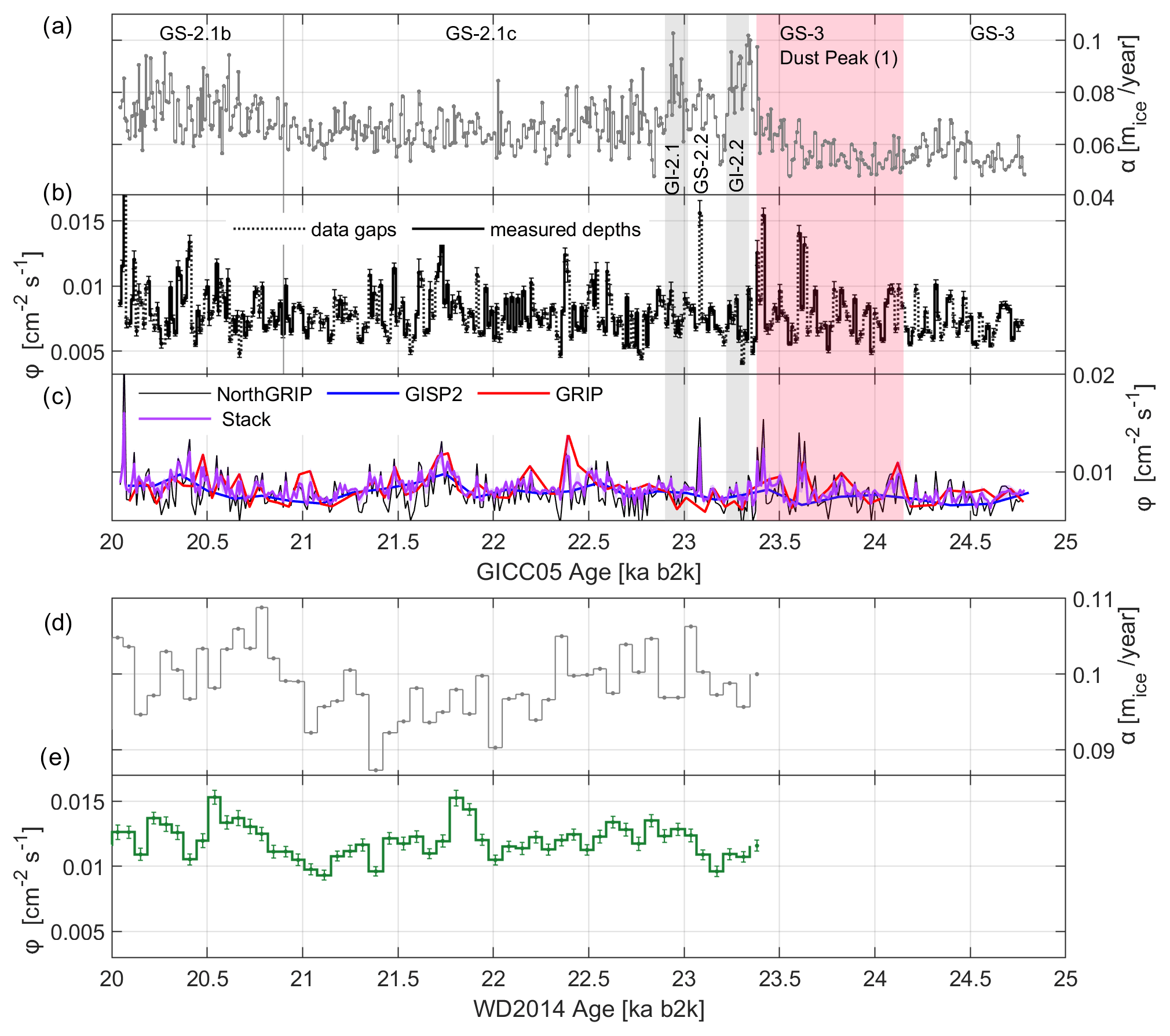
Figure 3 (a) The accumulation rate of NorthGRIP, downsampled to the same depth resolution of each ¹⁰Be data point. (b) The ¹⁰Be fluxes of NorthGRIP have an average of 0.008 ± 0.002 atoms cm⁻² s⁻¹. (c) Stack of the fluxes of the three Greenland ice cores, at 10-year resolution. (d) The published accumulation rate of WDC (Fudge et al., 2016), downsampled to the age resolution of the ¹⁰Be concentrations. (e) The ¹⁰Be fluxes of WDC average at 0.011 ± 0.001 atoms cm⁻² s⁻¹, higher than in Greenland, because of either depositional differences between the poles (Heikkilä et al., 2013) or accumulation rate inaccuracies.

Finally, an average of the ¹⁰Be fluxes of the three Greenland ice cores was calculated by stacking the NorthGRIP, GRIP, and GISP2 fluxes using Monte Carlo bootstrapping (Adolphi et al., 2018). The assumption behind averaging fluxes is that local accumulation effects are mostly removed by the conversion to fluxes and that the climatic effects on ¹⁰Be deposition are the same over Greenland. For each iteration, three of the data series are selected with resampling, and each dataset is perturbed within its uncertainties and averaged. The stack is shown in Fig. 3c.

2.4 Carbon-cycle modelling and uncertainties

The interaction of galactic cosmic rays (GCRs) with the atmospheric parent atoms (N, O) of ¹⁰Be and ¹⁴C is modulated by the time-varying helio- and geomagnetic fields. The radionuclides recorded in climatic archives ideally show synchronizable features in their production history (Steinhilber et al., 2012; Adolphi et al., 2018). The ¹⁴C atoms enter the carbon cycle, which causes delay and smoothing of the atmospheric ¹⁴C concentration relative to the production signal. However, the connection with the rapidly deposited ¹⁰Be in ice cores (1–2-year depositional delay; Raisbeck et al., 1981) can be made using a carbon-cycle model. Here, the box-diffusion model by Siegenthaler (1983) is applied to derive the atmospheric Δ¹⁴C signal, i.e. the decay and fractionation-corrected ratio of ¹⁴C $/$ ¹²C relative to a standard (Stuiver and Polach, 1977), from the measured ice-core ¹⁰Be. This model was used extensively in works by Muscheler et al. (2000, 2004, 2014), Muscheler (2009), Adolphi et al. (2014, 2018), and Adolphi and Muscheler (2016).

We assume here that any variations in ¹⁰Be in ice cores can be converted to a global ¹⁰Be production rate, proportional to the global ¹⁴C production rate. This assumption may, however, lead to uncertainties. For example, changes in the balance between wet and dry deposition or changes in the transport of ¹⁰Be to the ice sheet are possible factors that might alter the signal recorded in ice cores from the true production rate.

The ice-core ¹⁰Be is normalized relative to its mean, amplified by 20 % (as estimated below), and provided as input signal to the model. The model should run with parameters that best represent the state of the carbon cycle and its changes through time, with the assumption that any remaining variability will be related purely to production effects. However, as we do not know these carbon-cycle changes well enough, we keep in mind that the measured ¹⁴C may have been affected by changes in the carbon cycle that are not considered in the model, adding additional signals that are not related to production rate changes.

In the period 20–25 kyr b2k, the Hulu Cave Δ¹⁴C_calcite is about 500 ‰ (Fig. 2e), which is higher than early Holocene values, which are below 200 ‰ (Reimer et al., 2020). These higher values may be related to one or more of the following factors: a lower ocean diffusivity during the LGM or any process that similarly reduces the carbon uptake by the ocean (Muscheler et al., 2004), a lower atmospheric ¹²C inventory resulting in higher ¹⁴C $/$ ¹²C ratios (Köhler et al., 2022), or a weaker geomagnetic field. For instance, Muscheler et al. (2004) expect the ¹⁰Be production rates in the LGM to have been about 20 % higher than today, due to the lower geomagnetic field intensity during the LGM.

To determine the most appropriate model parameters, we repeat the calibration by Adolphi et al. (2018) around the Laschamps geomagnetic excursion at 41 kyr b2k, since the available ¹⁴C data have been updated since then (Reimer et al., 2020). We run the model with different ocean ventilation values (Fig. S1), finding that, for values of ocean diffusivity between 25 %–40 % of the pre-industrial Holocene value, the modelled Δ¹⁴C matches the IntCal20 data best. This is in agreement with Muscheler et al. (2004), who performed a time-dependent adjustment of the ocean diffusivity parameter between 10–25 kyr b2k. In their study, the LGM ocean diffusivity was set to ∼ 1000 m² yr⁻¹, about 25 % of the pre-industrial Holocene value.

In summary, we find that a 20 % production rate amplification of the normalized ¹⁰Be and an ocean diffusivity of 25 % of the pre-industrial Holocene value produce modelled outputs of about 500 ‰, in agreement with the Hulu Cave measurements, although the model fails to capture the decreasing trend. We note that this is not necessarily a realistic parametrization of the state of the carbon cycle, but it allows us to match some of the main features seen in the data. We associate no uncertainty with the model parameters since no set-up realistically explains all the Δ¹⁴C_calcite features.

To compare the measured and the modelled Δ¹⁴C, in this study we make use of linear detrending, as this largely removes the systematic offsets associated with the unknown carbon-cycle history and inventories. The detrending is performed by first selecting data in the 20–25 kyr b2k time frame and then using the MATLAB function “detrend”, which subtracts the best-fit line from the data. Some residual effect of the parametrization is observable in the amplitude of detrended Δ¹⁴C, but not in the timing of the changes, which is most important here.

Sensitivity tests: ocean diffusivity changes, accumulation rate uncertainties, measurement uncertainties

To provide an uncertainty boundary for the detrended modelled Δ¹⁴C curves, we performed three separate sensitivity tests. As a first test, we investigated how short-term changes in the ocean diffusivity affect the modelled output because during the LGM there likely have been changes in the carbon cycle around the GIs and the HS-2 (Bauska et al., 2021).

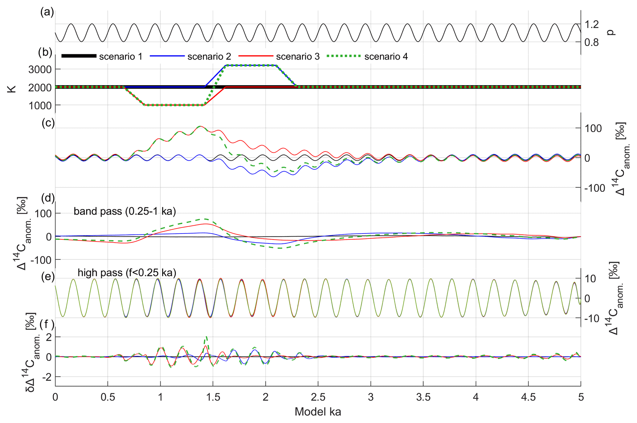
Figure 4 Sensitivity tests for time-dependent ocean diffusivity changes. (a) Normalized production rate input shaped as a periodic wave with an amplitude of ±25 % and a period length of 200 years, broadly consistent with typical solar de Vries cycle variability observed in ¹⁰Be (e.g. Wagner et al., 2001). (b) Scenarios of ocean diffusivity, as described in the text. (c) Model output, after linear detrending. (d) Long-term variations in the output (band-pass-filtered with periodicity of 250–1000 years). (e) High-pass-filtered output, up to 250-year periodicity, with amplitudes of around 20 ‰. (f) Differences in the high-pass-filtered curves in (e) between the control scenario 1 and the other three scenarios (similar to Adolphi and Muscheler, 2016).

A time-dependent change in ocean diffusivity was induced using three scenarios, as shown in Fig. 4b. The control scenario is set at 50 % of the pre-industrial value. We induce an abrupt increase in ocean ventilation (to 80 % of the pre-industrial value), an abrupt decrease (to 25 %), or a sequence of both. The duration of the events is chosen to reflect changes in the NorthGRIP calcium record, while the transition time was set to 200 years.

Figure 4c shows that the effects of the perturbations in ocean diffusivity on Δ¹⁴C span several tens of per mille after detrending. Thus, any feature in the ¹⁴C records that is in the proximity of an abrupt climate change and has a comparable duration is uncertain and should not be used for matching. On the other hand, Fig. 4e shows that short-term variations in the modelled Δ¹⁴C signal are less affected by the diffusivity perturbation. At least in principle, signals exceeding 10 ‰–20 ‰ that are much shorter than the climatic transitions could be used for wiggle-matching, since Fig. 4f shows that the different ocean diffusivity scenarios affect the high-passed Δ¹⁴C only within 2 ‰, hardly above measurement uncertainties.

A second sensitivity test was performed to investigate the effect of accumulation uncertainties related to the strain model. We performed two experimental model runs where we shifted the thinning function (inverse strain) by ±20 % of the mean value between 20 and 25 kyr b2k, which is a realistic modelling uncertainty between independent studies of the accumulation rate (Rasmussen et al., 2014; Gkinis et al., 2014). Changing the strain rate creates an uncertainty of about 3 ‰ between the modelled and detrended Δ¹⁴C curves, as shown in Fig. 5b. Furthermore, with a similar approach, we quantify the impact of ¹⁰Be measurement uncertainty on the modelled Δ¹⁴C to be 1 ‰ (Fig. S2). Adding these independent contributions in quadrature, we set an uncertainty for our modelled Δ¹⁴C of 5 ‰. This uncertainty serves as an initial parameter for the wiggle-matching algorithm, described in the next section; it furthermore agrees with the uncertainty adopted for the comparison of centennial variations in ¹⁴C and ¹⁰Be during the stable climate of the Holocene (Adolphi and Muscheler, 2016). However, as we have verified with our test, Δ¹⁴C changes in the vicinity of climate perturbations bear a considerably higher uncertainty.

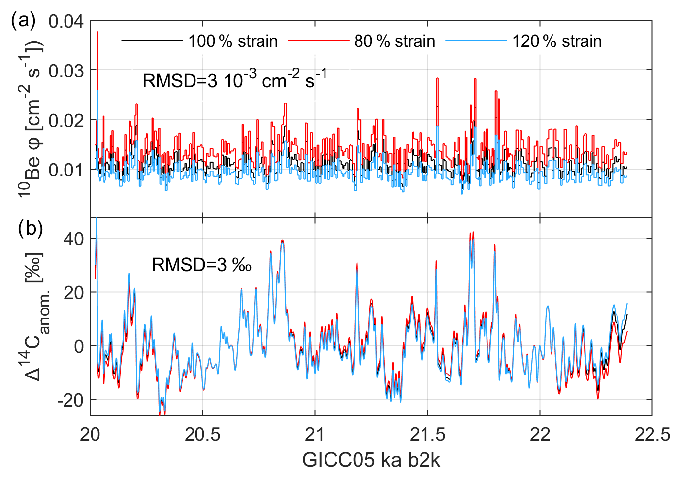
Figure 5 Sensitivity test of the effects of accumulation-related uncertainties on the carbon-cycle modelling. (a) Two strain-model scenarios produce different flux values. (b) The modelled Δ¹⁴C curves are detrended, which largely removes the differences between the scenarios. However, the RMSD between the curves, 3 ‰, represents the remaining variability.

2.5 The wiggle-matching algorithm reproduced from Adolphi and Muscheler (2016) and its uncertainty

A wiggle-matching algorithm, adapted by Adolphi and Muscheler (2016) from the original formulation by Bronk Ramsey et al. (2001), represents an important tool for the quantification of offsets between timescales, along with visual inspection. The first input for the algorithm is the detrended Δ¹⁴C modelled from the ice-core ¹⁰Be. The second input is the detrended Δ¹⁴C_calcite data from the Hulu Cave stalagmite samples. The output of the algorithm is a probability density of the timescale offsets, t_offset.

Following the approach by Adolphi and Muscheler (2016), we do not allow for stretching of the underlying chronologies. We investigated the offset probability within partially overlapping time windows W, spaced every 50 years, obtaining a two-dimensional probability matrix P(W, t_offset). We summarize the algorithm settings in the Appendix.

The most likely offset, $t_{\mathrm{offset}}^{\ast }\left(\mathit{W}\right)$, is defined here as the maximum of P. We identify the boundaries T1 and T2 between which $t_{\mathrm{offset}}^{\ast }\left(\mathit{W}\right)$ is stable, and we calculate an average offset.

After shifting each ice-core dataset by the proposed offset, we computed the χ² test between the Δ¹⁴C curves. If the p value was outside the 0.01–0.99 interval, we repeated the wiggle-matching using the standard deviation of the residuals (RMSD in ‰) as the uncertainty for the modelled Δ¹⁴C curve. We re-evaluated the boundaries T1 and T2 and re-averaged the $t_{\mathrm{offset}}^{\ast }$ curves, obtaining a final estimation for the offset.

We aim to establish an uncertainty in the offset that considers the uncertainties in both ice-core and speleothem timescales, as well as resolution limitations. We therefore applied a Monte Carlo protocol to estimate the uncertainty and conducted the following steps:

1. For each modelled Δ¹⁴C dataset and window W^∗, we approximate the $\mathbf{P}(W^{\ast },{\mathit{t}}_{\mathrm{offset}})$ as a Gaussian distribution, with 1σ as the average lower and upper width at half maximum of $\mathbf{P}(W^{\ast },{\mathit{t}}_{\mathrm{offset}})$. By arbitrarily choosing the mode of P as the best offset, we can disregard any other lobe of probability as spurious, with high confidence given by our visual inspection of the data.

2. For each dataset and window W^∗, we sample randomly from the Gaussian 10 000 times to derive an ensemble of timescale offsets.

3. By iterating steps 1 and 2 across all datasets and all windows within the established time boundaries T1 and T2, we compute the overall histogram of the sampled offsets.

4. We evaluate the 68 % confidence interval of this histogram around the best offset established as the mode.

This procedure is repeated separately for WD2014 and GICC05 and also for the Hulu H82 and MSD datasets. The algorithm is available in the Supplement.

3 Results

3.1 A promising inter-ice-core tie point for ¹⁰Be synchronization

Previously used for the matching by Adolphi et al. (2018), a ¹⁰Be increase at 21.7 kyr b2k (GICC05 age) is visible in the new NorthGRIP data as well as in the WDC dataset (Fig. 2). This radionuclide increase resembles the ¹⁰Be signal associated with the Maunder Solar Minimum (1645–1725 CE), which was a period of low solar activity and consequent increase in the global radionuclide production (Berggren et al., 2009; Eddy, 1976). In Fig. 6, we compare the Holocene and LGM counterparts of ¹⁰Be at NorthGRIP, finding similar shapes and duration. This supports the attribution of the ¹⁰Be increase to a solar minimum during GS-2, which could explain the co-registration across ¹⁴C_calcite and ¹⁰Be datasets.

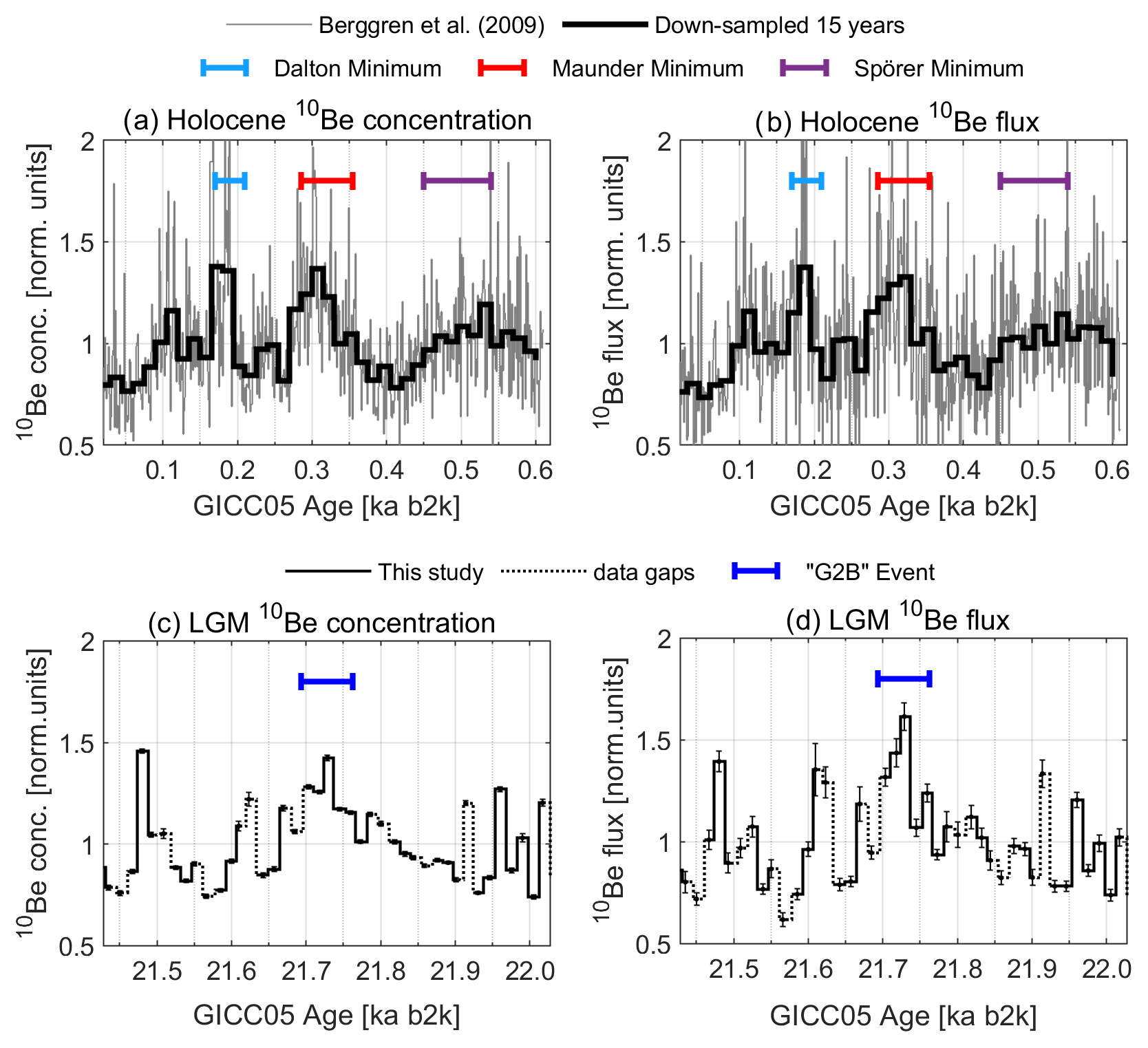
Figure 6 Comparison of ¹⁰Be ice-core data in the Holocene, around the Maunder Minimum, and in the LGM, around the G2B event. Data were divided by the mean within ±300 years of the central event. (a, b) In the Holocene, the NorthGRIP ¹⁰Be data by Berggren et al. (2009) compare well to the defined durations of the grand solar minima, which were independently recorded in the sunspot observations. An increase in the ¹⁰Be production rate by about 40 %–50 % from the average is produced by the solar minimum. The fluxes show a more abrupt increase in time, while concentrations record a more gradual increase. (c, d) In the LGM, the similarity of shape and duration to the Maunder Minimum supports the identification with a solar minimum.

Based on the observed similarities in Fig. 6, we call the 21.7 kyr b2k increase the “GS-2.1c ¹⁰Be event” (abbreviated G2B event in the following). To support the bipolar synchronization, after resampling the NorthGRIP ¹⁰Be data at the resolution of WDC, we observe that the two ice cores register similar ¹⁰Be amplitudes around the G2B event. The flux increases by 0.003 atoms cm⁻² s⁻¹ at both sites, which represents an increase of 40 % and 30 %, respectively, from the flux average values at NorthGRIP and WDC. The ¹⁰Be concentration, on the other hand, increased only 30 % (1.3 × 10⁴ atoms g⁻¹) and 20 % (0.9 × 10⁴ atoms g⁻¹), respectively, from the concentration average values at NorthGRIP and WDC.

3.2 Synchronization between ice cores using ¹⁰Be

Having established the G2B event as a radionuclide production feature, we can synchronize Greenland ice cores by inserting new ¹⁰Be tie points between NorthGRIP, GRIP, and GISP2. Furthermore, the G2B event can be used to improve the bipolar matching to Antarctica (Fig. 7).

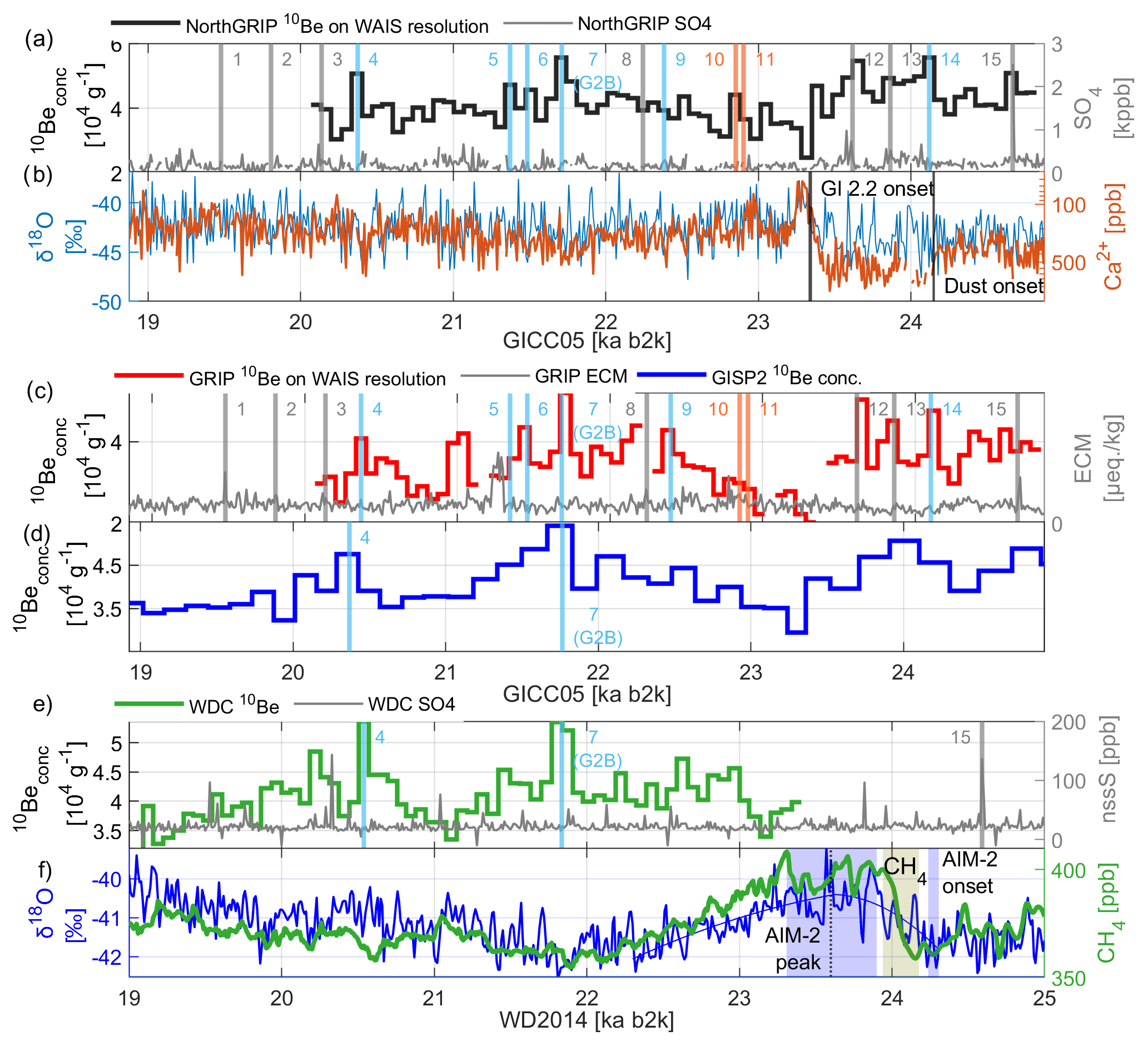
Figure 7 Bipolar tie points and climatic proxies. Vertical bars indicate the type of tie points (grey: volcanic; blue: ¹⁰Be; orange: ammonium). The data were aligned using tie point 7 (G2B event), without stretching the chronologies. (a) The NorthGRIP tie points are based on ¹⁰Be (black), sulfate data (grey), and ammonium data (not shown). (b) NorthGRIP δ¹⁸O_ice and Ca²⁺ (inverted log scale) qualitatively represent the climate in the LGM. (c) The GRIP tie points are based on ¹⁰Be (red), electrical conductivity measurement (ECM; grey), sulfate (not shown), and ammonium (not shown). (d) The ¹⁰Be data of GISP2 (blue) have a low resolution. Tie point nos. 4 and 7 are however sufficiently visible in the data. (e) WDC ¹⁰Be data (green) and nssS (grey; no. 15 by Svensson et al., 2020). (f) WDC climatic proxies, with CH₄ presented in the gas chronology by Buizert et al. (2015). The ages of the AIM-2 onset and peak and of the methane increase are described in the text.

We decided to compare the ¹⁰Be data at similar resolutions to facilitate the identification of other common production features. Hence, we downsampled the high-resolution data of NorthGRIP to the same resolution as GRIP and WDC, since ice-core ¹⁰Be measurements are averages over the sampling depth intervals and lose variability with decreasing resolution.

Figure 7 shows the ¹⁰Be concentrations from NorthGRIP, GRIP, and WDC on their respective chronologies, together with a set of published tie points (Seierstad et al., 2014; Svensson et al., 2020). Between NorthGRIP and GRIP, we observe important similarities in the ¹⁰Be data, which leads us to suggest six new ¹⁰Be tie points: a peak at 20.4 kyr b2k, a double peak at 21.5 kyr b2k, the G2B event at 21.7 kyr b2k, a single peak at 22.4 kyr b2k, and a triple peak structure between 23.5 and 24.2 kyr b2k. These tie points cover the previously tie-point-free section across GS-2.1b/c.

Table 2 ¹⁰Be tie point ages between NorthGRIP, GRIP, and WDC. The internal difference between the Greenland ice cores (δ) reaches 27 years at the G2B event. Likewise, the difference between WDC and NorthGRIP ages (Δ) indicates older ages for WDC at the G2B event and the youngest no. 4 tie point.

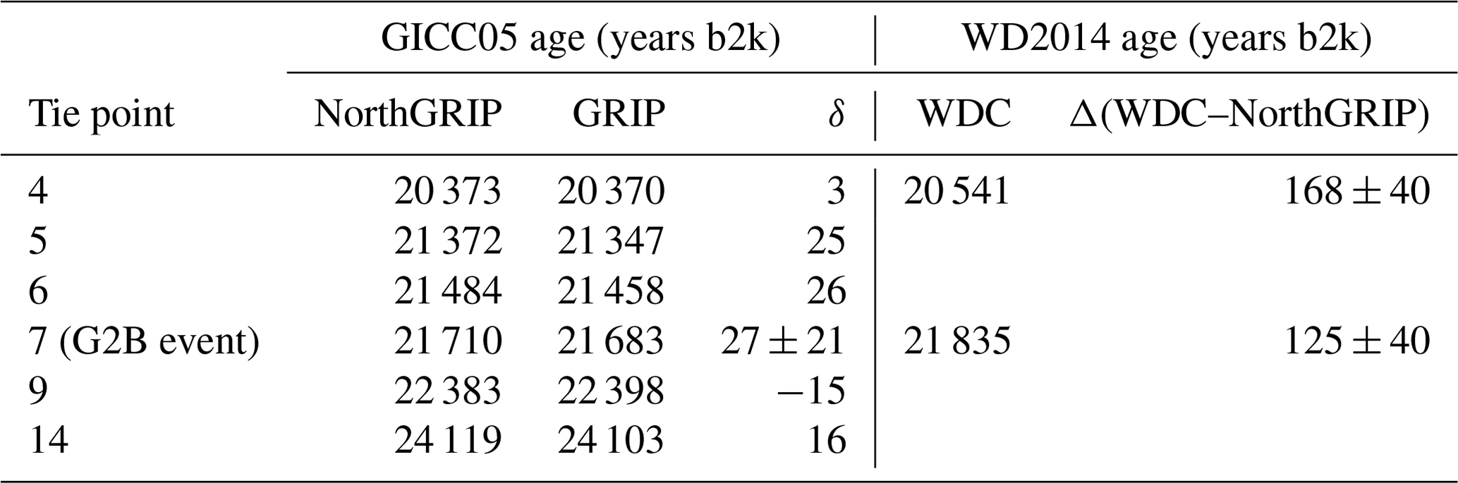
The tie points to WDC, of which Svensson et al. (2020) published the oldest (no. 15), are extended with the aid of two additional ¹⁰Be tie points (nos. 4 and 7/G2B). The choice of no. 4 as a bipolar tie point is motivated by a similar layer count of ∼ 1300 years from G2B and a similar shape of the signals. The ages of the tie points are summarized in Table 2 and derived from the mid-depth of the highest peak.

The timescales of GRIP and NorthGRIP are slightly misaligned between 21 and 23 kyr b2k by up to 27 years at the G2B event, probably because GRIP ages were interpolated between widely spaced tie points. The uncertainty in this misalignment can be estimated as half the sum of the resolutions of NorthGRIP and GRIP measurements (±21 years, 1σ), as this is likely to limit our matching precision in each direction. Therefore, ¹⁰Be measurements cannot be said to resolve matching issues between Greenland ice cores with very high precision; nonetheless we use the new ¹⁰Be tie points in the following to produce an updated accumulation rate for GRIP. Furthermore, WD2014 and GICC05 are misaligned by 125 ± 40 years at the G2B event, WD2014 being older; the uncertainty in this offset is given as half the sum of the resolutions of WDC and NorthGRIP data.

The fact that the G2B event is 27 years older in NorthGRIP than GRIP means that the GRIP timescale and the accumulation rate need to be corrected because the new tie points induced a change in the layer thickness. Hence, we calculated a new depth–depth interpolation between the two Greenland ice cores, and we assigned an updated age scale to the GRIP depths. The corrected accumulation of GRIP was computed by multiplying its layer thickness by a correction function of the relative change between the tie points. For example, since NorthGRIP has 1235 layers between tie point nos. 4 and 7, while GRIP only has 1210 layers, the correction factor for the accumulation rate between these tie points is 1.02. Due to these relatively small corrections, we do not find it necessary to apply any smoothing to the correction function. In the following, we denote fluxes of GRIP that were corrected in this way as “corrected fluxes” when we need to distinguish them from the previous version used by Adolphi et al. (2018). Although the effect of the accumulation correction is small, it has an impact on the amplitude of the G2B event signal in GRIP, making the NorthGRIP- and GRIP-modelled Δ¹⁴C curves look more alike. At the resolution of the GISP2 dataset, ¹⁰Be appears to be sufficiently aligned around the G2B event and the peak at 20.4 kyr b2k; hence no age correction was applied to GISP2.

In Fig. 7b and f, selected climatic proxies are shown to illustrate that a bipolar match across the LGM is already sufficient to change the timing between the two GIs and the AIM-2, bringing the AIM-2 closer to the GI-2.2 onset (a “before version” of the alignment of the climatic proxies is shown in Fig. 1).

In the WDC isotope data, we fit a curve to the δ¹⁸O_ice record over the AIM-2 period to determine both the likely age for the onset of the warming slope and the peak – all on the original WD2014 chronology. We used the MATLAB function “WDC_breakpoint” provided by WAIS project members (2015), which fits the AIM with a double-polynomial fit, to identify the maximum. However, the fit is sensitive to the starting guess for the position of the maximum; by varying the starting guess between 23 and 25 kyr b2k, we observed that the fit finds several maxima. This fact is attributed to the shape of the signal being ambiguous and very broad. Moreover, a visual maximum of the AIM-2 is clearly identifiable at 23.6 kyr b2k. Taking this as the central estimate, we estimate the location of the AIM-2 peak as 23 600 ± 300 years b2k (1σ). On the other hand, the onset of the AIM-2 is more easily defined to be 24 272 ± 35 years b2k (1σ).

Table 3 Event onsets and terminations discussed in this work, corrected for the timescale offsets, with 1σ confidence intervals. In the “Original calendar age” column, the onset of GIs and dust terminations are based on the original definition by Rasmussen et al. (2014) with reported uncertainties related to the event definition only. The dating uncertainty is dominated by the uncertainty in GICC05, which is about 600 years at this age. The ages of the AIM-2 and CH₄ increase in WDC were assessed as described in the main text. In the column “Age according to wiggle-matching synchronization”, GICC05 has been shifted by ${\mathrm{375}}_{-\mathrm{300}}^{+\mathrm{250}}$ years, while the WD2014 ages were shifted by ${\mathrm{225}}_{-\mathrm{250}}^{+\mathrm{200}}$ years, both towards older ages. The uncertainty in the new age was propagated from the original uncertainty and the offset uncertainty, using the asymmetric 1σ boundaries of the offset.

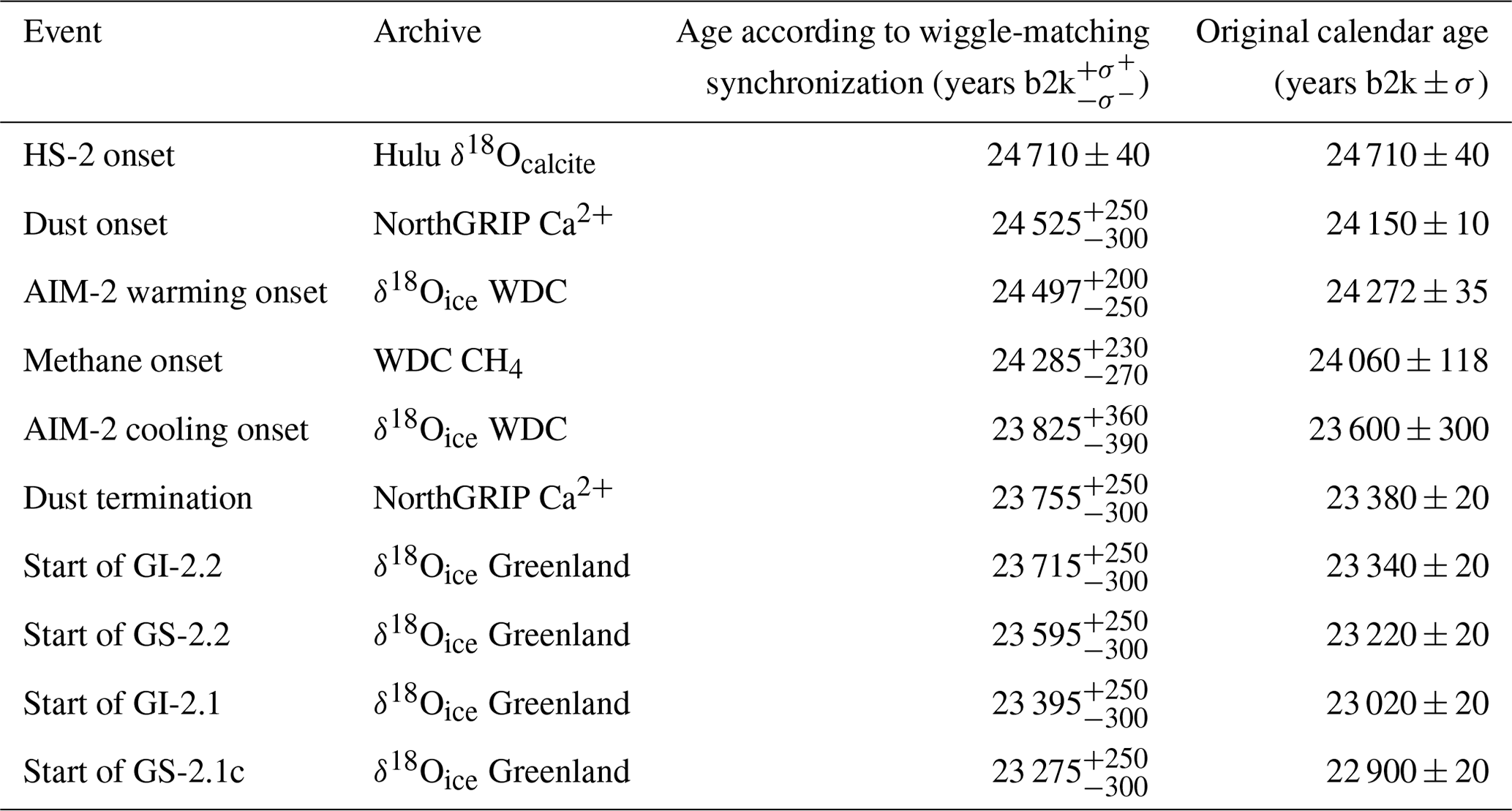
The onset of the CH₄ increase at 24 060 ± 118 (1σ) years b2k is defined as the instant at which the signal becomes higher (and remains higher) than 1 standard deviation from the average baseline of the period 24.5–25.5 kyr b2k. The uncertainty in the CH₄ onset is quoted from the gas age uncertainty in WD2014 (Buizert et al., 2015), which is mostly useful to compare CH₄ to the δ¹⁸O_ice signal of the same ice core, WDC. All values are summarized in Table 3.

By aligning the two ice-core timescales at the G2B event, and without stretching the chronologies, we shift the GICC05 data by 125 years compared to WD2014 data. We observe that the AIM-2 peak now happens 125 years before the onset of GI-2.2, instead of 250 years before, as was the case on the original timescales. The alignment at the G2B event is not sufficient to alter the order of the GI-2–AIM-2 sequence. What the new alignment shows is that the AIM-2 warming occurs within the dust peak and that the AIM-2 cooling occurs with the dust peak termination in Greenland, with potential influence of the GIs.

3.3 Carbon-cycle modelling and wiggle-matching

Inspection of the measured Δ¹⁴C_calcite (Fig. 8a) and the ¹⁰Be-based Δ¹⁴C (Fig. 8b, c, e) confirms the expectation that a shift in the two ice-core chronologies towards older ages is required for a better alignment with the Hulu Cave ¹⁴C_calcite record.

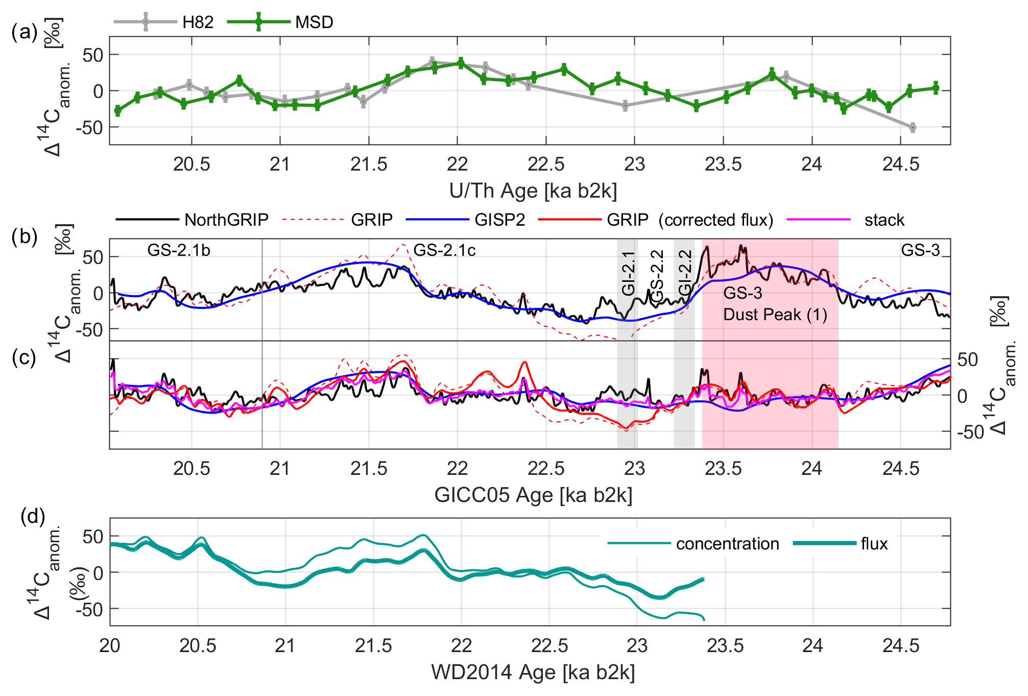
Figure 8 Carbon-cycle-modelled Δ¹⁴C compared to measured Hulu Cave data, before synchronization. (a) Hulu Cave Δ¹⁴C_calcite. (b) Modelled Δ¹⁴C from Greenland ¹⁰Be concentrations. (c) Modelled Δ¹⁴C from Greenland ¹⁰Be fluxes, including the flux stack (magenta). The effect of the flux correction of GRIP is mostly visible around the G2B event, where the corrected data (solid red line) show a better agreement with the other cores. (d) Δ¹⁴C modelled from WDC ¹⁰Be fluxes and concentrations.

We observe two non-climatic tie points between all Δ¹⁴C curves:

1. A relatively abrupt increase of 30 ‰ is observed in the modelled Δ¹⁴C at 21.7 kyr b2k (GICC05 ages). The most likely equivalent of this event is observed in the Hulu Cave data at around 22 kyr b2k (U $/$ Th ages), where an increase of about 25 ‰ happens abruptly between two data points, which is followed by a slow decrease. In the H82 data by Southon et al. (2012), the increase is much less abrupt and spans four data points.

2. A 40 ‰ peak is observed in the ice-core Δ¹⁴C at 20.4 kyr b2k (GICC05). In Hulu Cave data, one elevated data point at 20.8 kyr b2k (U $/$ Th) is visible in the MSD dataset, but the H82 record does not show this peak.

We assume that the modelled and the measured Δ¹⁴C should, after detrending, be dominated by the same production signal and that the differences we observe in the datasets can be explained by noise, modelling uncertainties, and dynamics affecting the deposition rather than the production of the radionuclides. Therefore, we proceed with the wiggle-matching despite the observed differences.

Based on these considerations, we run the wiggle-matching algorithm exclusively in the 20.5–22.5 kyr b2k range (U $/$ Th ages), using data windows of 1300 years with an overlap of 50 years between successive windows. The 1300-year choice is motivated by a compromise between enough signal inclusion in each window and more precision, since preliminary tests showed that this value returned the most stable results, compared to windows of 1000 or 1500 years. For the U $/$ Th timescale, we use both Hulu datasets, but we separate our treatment for the H82 and the newer MSD data (Southon et al., 2012; Cheng et al., 2018) because of the different resolution and the slightly different signals recorded. For the WD2014 timescale, we use both the WDC ¹⁰Be concentrations and fluxes, modelled to Δ¹⁴C, since they are similar after carbon modelling. For the GICC05 timescale, we use all available Δ¹⁴C modelled from concentrations, fluxes, and the flux stack, since they are similar at least around the production features we are going to match.

By averaging the obtained offset curves across the datasets and the interval (Fig. S4), we estimate the chronological offset to be 375 years for GICC05 and 225 years for WD2014, using the MSD dataset exclusively. We do not give an uncertainty boundary for these offsets just yet, as we first perform a χ² test, following the protocol outlined in the Methods section. We evaluated the χ² and the associated p value between each shifted Δ¹⁴C curve and the Hulu dataset. For the flux-based datasets, the p values were within the 0.01–0.99 threshold, except for the GRIP “uncorrected” fluxes. This last exception motivates the exclusion of “uncorrected” fluxes in the following, as we do not need to keep both GRIP flux-based curves once we have ascertained that the “corrected fluxes” satisfy our χ² test, possibly because of the improved chronological spacing of the samples.

In the case of all Greenlandic concentration-based curves, because of very low p values of the χ² (p ≪ 0.01), we decided to set the modelled-Δ¹⁴C uncertainty to the RMSDs of each dataset, which are between 12 ‰ and 21 ‰, less than the amplitude of the matched features. We repeat the wiggle-matching for these cases and base our offset estimation on the full Greenland dataset with the uncertainty method outlined above.

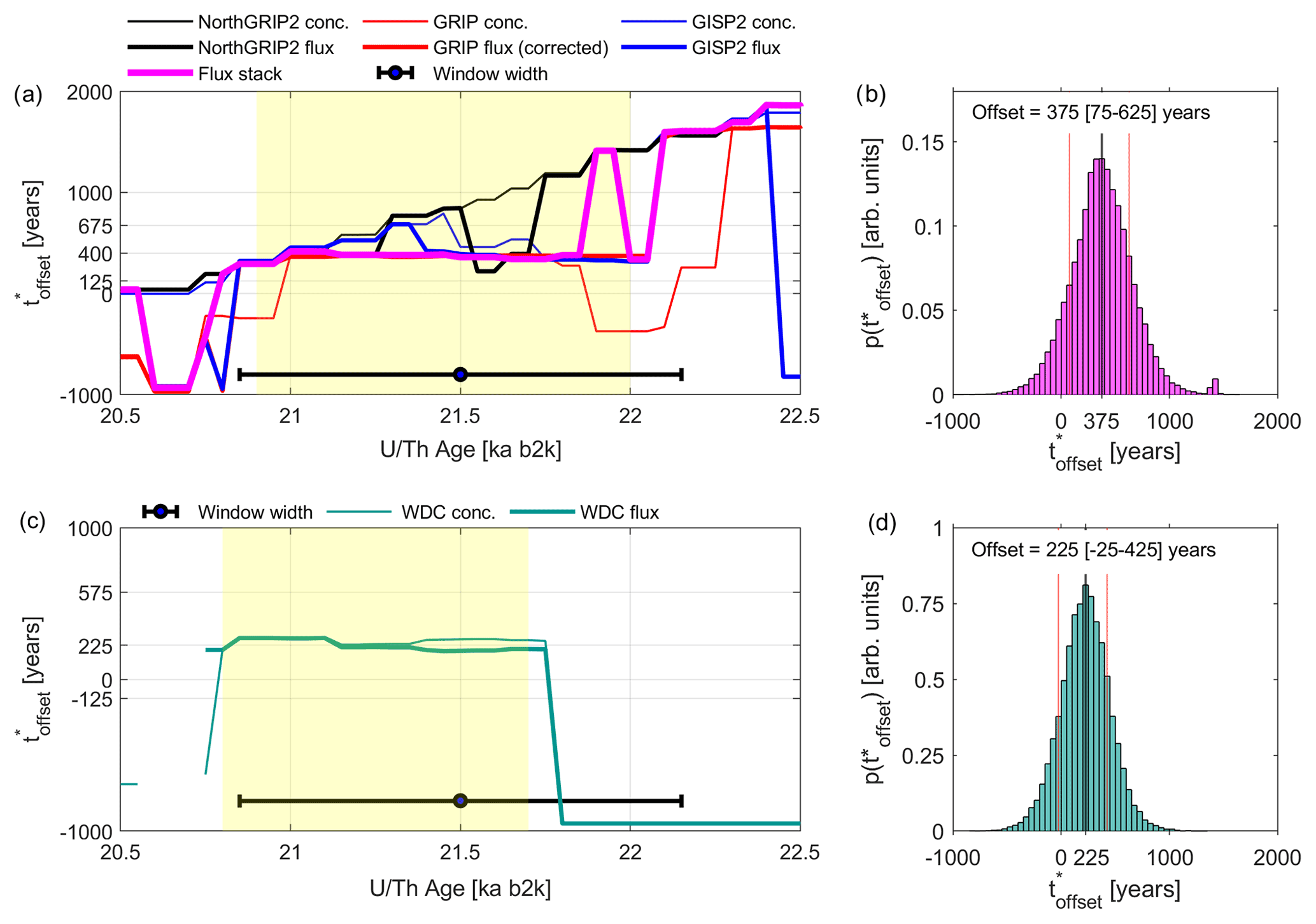
Figure 9 Wiggle-matching and Monte Carlo results around the G2B event for Greenland (a, b) and the WDC core (b, c). MATLAB code is provided in the Supplement. The curves in the left panels are the timescale offset $t_{\mathrm{offset}}^{\ast }\left(\mathit{W}\right)$ of each ice-core dataset. The yellow area delimits the time intervals for averaging (T1 and T2), outside of which curve instability is caused by the lack of appropriate matching features in the data. (b) Distribution of the Greenland offset. From the histogram, we compute the 68 % confidence interval of the offset (red lines). (d) Distribution of the WDC offset, with 68 % confidence bars.

We therefore repeat the averaging of the timescale offset (Fig. 9) between the MSD dataset and the GICC05 ensemble, and we apply the Monte Carlo iteration outlined in the Methods, between 21 and 22.1 kyr b2k (the range highlighted in yellow in Fig. 9a, where edge effects can be avoided). We obtain the offset estimate of 375 years, a 68 % confidence interval from 75 to 625 years, and a 95 % confidence interval from −300 to 1000 years. One assumption behind this approach is that the offset should only change slowly with time, which is supported by the flatness of most curves in Fig. 9 (with some exception by the concentration-based offsets of NorthGRIP and GISP2).

For the WDC datasets, both flux- and concentration-based curves were shifted by 225 years. Upon performing the χ² test against the Hulu Cave data, the p values were within the 0.01–0.99 tolerance interval; hence the uncertainty in the modelled Δ¹⁴C data did not need to be re-evaluated. We compute the average timescale offset (Fig. 9) between the MSD dataset and the WD2014 ensemble of flux- and concentration-based curves, and we apply the Monte Carlo iteration outlined in the Methods section, between 20.8 and 21.75 kyr b2k (the range highlighted in yellow in Fig. 9b). We obtain the offset estimate of 225 years, a 68 % confidence interval from −25 to 425 years, and a 95 % confidence interval from −350 to 750 years.

The difference between the ice-core offsets represents another indirect estimate of the offset between the Greenland and Antarctic chronologies, which in this way is determined to be 150 years, close to the offset of 125 ± 33 years directly obtained by synchronizing the G2B event in the ¹⁰Be fluxes.

Our result for GICC05 is smaller than the 550-year offset obtained by Adolphi et al. (2018) but fully consistent within the uncertainties in their estimate (95 % probability interval: 215–670 years). For the H82 dataset, our analysis leads to offsets of about 500 ± 200 and 220 ± 500 years, for GICC05 and WD2014, respectively, which more closely reproduces the Adolphi et al. (2018) finding.

4 Discussion

4.1 Climate compared after synchronization

In Fig. 10 we show the radionuclide and climatic data after the synchronization proposed in Sect. 3.3.

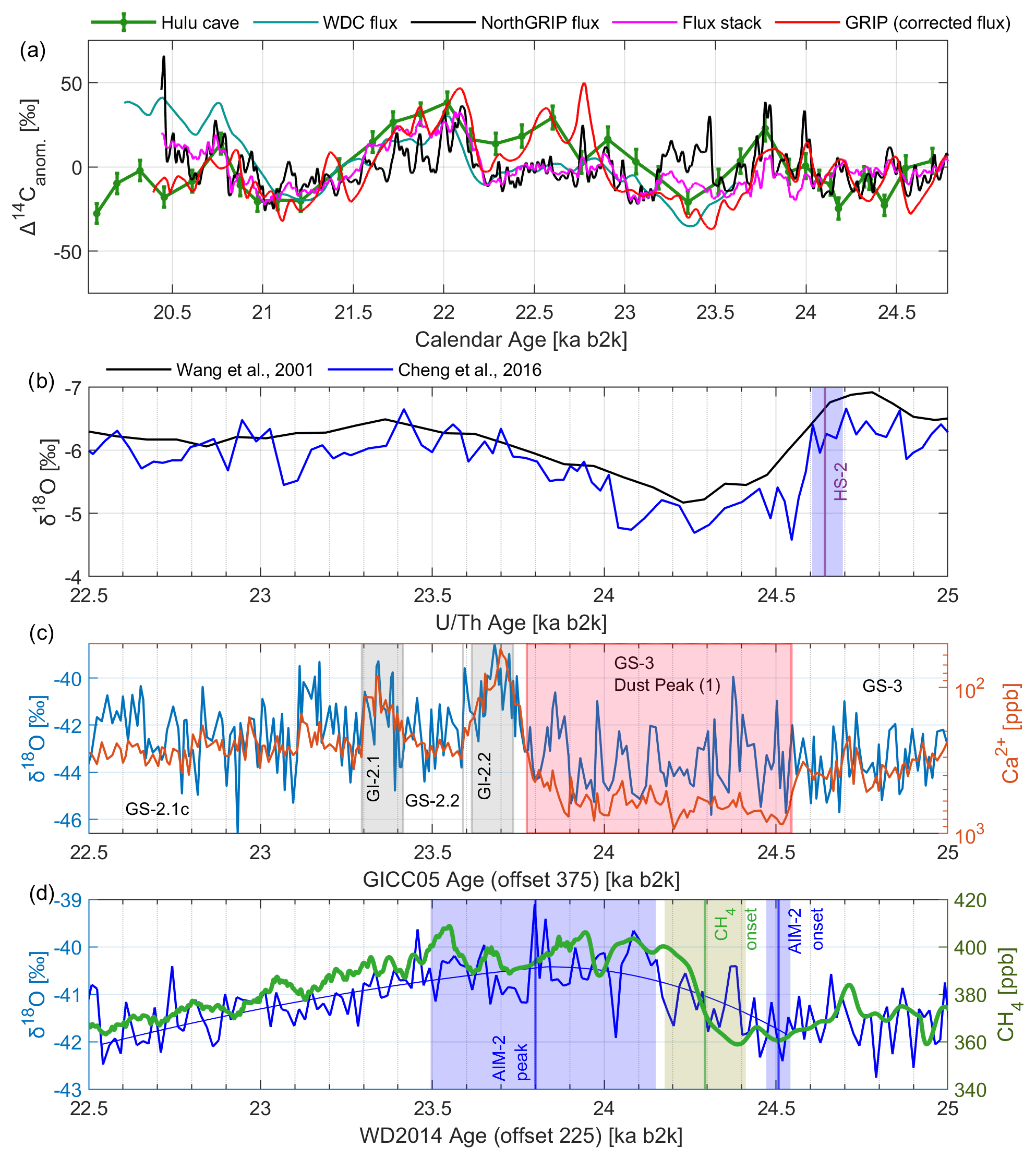
Figure 10 Radionuclide and climatic data after the synchronization. The Greenlandic records were shifted by 375 years towards older ages; the WDC records were shifted by 225 years towards older ages. (a) Radionuclide data used for wiggle-matching plotted on the synchronized timescales. (b) Hulu Cave isotopes (reversed y axis) highlight the suggested onset of HS-2 (Cheng et al., 2016). A lower-resolution dataset is also plotted for comparison (Wang et al., 2001). The termination of HS-2 is not defined, as multiple possibilities arise by comparing the two datasets. (c) Greenlandic proxy data on the shifted GICC05. (d) WDC proxy data on the shifted WD2014.

To reconstruct the sequence of events during the LGM, we need to estimate the onset and termination of HS-2. We suggest the onset of HS-2 to be defined by the δ¹⁸O_calcite slope in Asian speleothems (Fig. 10b; Cheng et al., 2021). Here, we identify the onset of the HS-2 signal at Hulu Cave by the same methods used for the AIM-2, combining the WDC_breakpoint function with a Monte Carlo iteration. By averaging the onset in the two δ¹⁸O_calcite onsets at Hulu Cave, one for each dataset, we obtain the HS-2 onset to be 24.71 ± 0.04 kyr b2k. This is earlier than an HS-2 onset at around 24.48 ± 0.08 kyr b2k (albeit compatible within 2σ with the definition by Li et al., 2021, thereof), based on another speleothem (Furong, China). The Hulu onset is also earlier than the Cherrapunji HS-2 onset at 24.47 ± 0.04 kyr b2k (Dong et al., 2022).

With the timescale correction for WD2014, the onset of the AIM-2 warming occurs synchronously with the HS-2 onset, within the uncertainties determined by both the wiggle-matching and the AIM-2 fit. A delay could be expected given the centennial-scale response of Antarctic climate to Northern Hemisphere changes (Pedro et al., 2018; Svensson et al., 2020).

The AIM-2 maximum (i.e. the peak of δ¹⁸O_ice in Antarctica) was defined here by considering only the data from WDC. By visual inspection, the peak of the AIM-2 signal could be identified either as two marked δ¹⁸O_ice peaks at around 23.8 kyr b2k (shifted WD2014 age) or as a prolonged plateau between 23.5 and 24.2 kyr b2k. We observe that the 23.8 kyr b2k peak in WDC occurs together with or slightly before GI-2.2, which is a similar result to that one obtains by merely synchronizing the data using the G2B event tie point (Fig. 7).

The shape of the AIM-2 signal differs across Antarctic ice cores (EPICA Community members, 2006), possibly because of registration differences across the continent. A comparative study of all Antarctic deep ice cores would improve our identification of the AIM-2, but the WD2014 timescale was only tied to few ice cores so far. At least we can compare the recent South Pole ice core (SPICE), chronologically tied to the WD2014 (Winski et al., 2019). The shape of the AIM-2 in SPICE is similar to WDC (Fig. S5). While the onset occurs at the same age, the maximum is reached earlier in SPICE, at 24.1 kyr b2k in the shifted WD2014 ages. This indicates that careful consideration of the geographic factors of the Antarctic continent are needed for an ultimate climate reconstruction of the AIM-2. In the meantime, we suggest that caution is exercised when interpreting minor isotopic signals.

The methane increase in WDC is registered ∼ 210 years after the AIM-2 warming started and after the HS-2 onset. This supports the theory by Rhodes et al. (2015) of an increased southern biogenic methane production as a delayed response to extreme northern-hemispheric cooling. The high methane levels appear to last between 460 and more than 1000 years, depending on how one defines the end of the methane plateau.

4.2 Discussion on causes of the offset for GICC05

In recent work by He et al. (2021), it was suggested that, although not reflected by Greenlandic water isotope records, a shutdown of the AMOC likely occurred during Heinrich Stadial 1, which was stronger than the AMOC shutdown of a “regular” GS, producing a period of extreme winter cooling. They concluded that, rather than Greenland not experiencing any additional cooling during HS-1 (as proposed by Landais et al., 2018), the imprint of the cooling in the δ¹⁸O_ice signal was cancelled by the effect of having less winter snow and by an increase in the δ¹⁸O_ice level of summer snow, due to the first warming of the deglaciation. The flatness in the water isotope data is, in their analysis, the result of these counteracting effects of Greenland cooling: the HS-1-specific reduction in winter precipitation and the ¹⁸O-enriched summer precipitation.

As far as the GICC05 layers are concerned, He et al. (2021) model a possible scenario over Greenland with a drastic decrease in winter precipitation by about 50 % at the onset of HS-1. On the other hand, they predict the summer precipitation to increase steadily as the deglaciation progresses, which is largely unaffected by the AMOC shutdown. This could potentially have produced thin and irregular layers at the onset of HS-1, with the summer part of the layer gradually increasing over time.

Acknowledging the 125-year offset between GICC05 and WD2014 at 22 kyr b2k and the 375-year offset between GICC05 and the U $/$ Th chronology, we proceed by discussing where the offset could have originated. According to Adolphi et al. (2018), the transfer function from GICC05 to IntCal is near zero at 13 kyr b2k, the closest tie point younger than the G2B event. Occurring between these two time horizons, the HS-1 period lasted from about 18 to 14.7 kyr b2k and is most often regarded as ending at the onset of GI-1. The authors of GICC05 retained the prior subdivision of the corresponding stadial, GS-2.1, in three sections (termed a, b, and c), of which GS-2.1a starts at 17.48 kyr b2k and ends at the onset of GI-1 (Björck et al., 1998; Rasmussen et al., 2014). The onset of GS-2.1a was originally defined by a second-order water isotope dip but occurs synchronously with an increase in the Greenland ice-core calcium profiles at roughly 17.6–17.4 kyr b2k.

If GICC05 missed a large number of annual layers across HS-1, the age of the onset of GS-2.1a would move towards older ages by a similar amount. We speculate that the onset of GS-2.1a could correspond to the onset of HE-1 (and thus the HS-1 period) and that calcium could be used as a signature of the change in atmospheric circulation influencing dust transport to Greenland during HS-1 as well as HS-2.

Part of the undercounted layers could have contributed to the uncertainty in GICC05. This was assessed by identifying so-called “uncertain annual layers”, that is, features that could be annual layers but are not clearly identified as such. Each uncertain layer contributed to the chronology and to the maximum counting error (MCE) as 0.5 ± 0.5 years (Rasmussen et al., 2006). Within GS-2.1a, the MCE grows by ∼ 150 years, meaning that 300 uncertain layers were identified as 0.5 ± 0.5 years. If we assume that all the uncertain annual layers in GS-2.1a were annual layers, an additional 150 years would appear in the chronology across this section.

As we have seen, according to He et al. (2021), a large number of very thin annual layers is a plausible scenario at least in the first part of HS-1, until the increasing summer precipitation alleviated the problem. As these layers are possibly unresolvable by the data, they would not be counted as uncertain layers; hence the MCE probably does not faithfully represent the full GICC05 uncertainty in sections where layer thicknesses are very small compared to the resolution of the data.

In addition to misassigned uncertain layers and layers missed altogether due to marginal data resolution, we propose here another explanation of what could have caused the undercount of GICC05 layers. The layers that are on the higher end of the thickness distribution, even if they were classified as “certain”, might indicate where very low or absent winter precipitation could have made multiple annual layers appear as one.

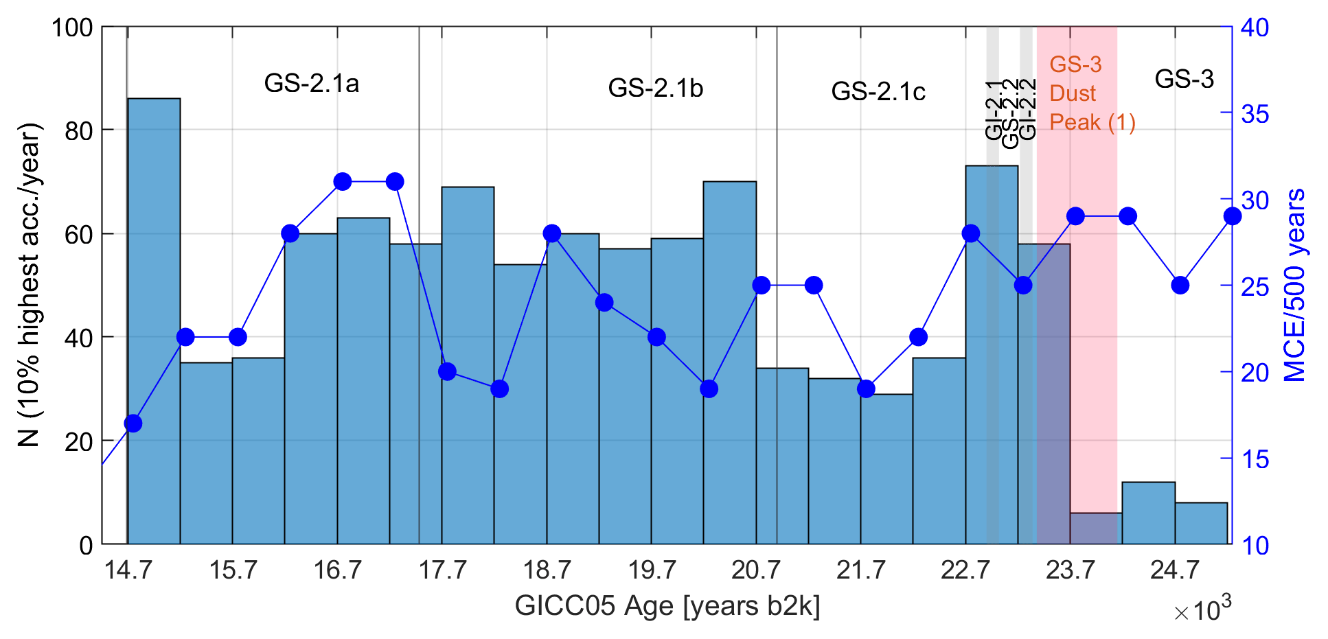
Figure 11 Highest-accumulation years (histogram) and MCE (dark-blue curve) based on the GICC05 timescale, computed on the same 500-year intervals.

To identify multiple layers, we highlight the years with highest accumulation in Fig. 11, where we also show the MCE, both per 500-year interval. The accumulation threshold is set at 0.09 m yr⁻¹ by integrating the highest 10 % of the accumulation distribution between 14.7 and 25 kyr b2k. The histogram in Fig. 11 thus shows the number of very thick layers in each time bin.

The thickest layers across GS-2.1b and GS-2.1a have as many high-accumulation years as interstadial periods, which is surprising given that this period was very cold and had very low annual precipitation (Kindler et al., 2014).

For the MCE, observers of GICC05 encountered more issues at the onset of GS-2.1a, whereas the MCE stayed constant over the rest of GS-2.1. Hence, we suggest that a dating bias could have accumulated across GS-2.1a and GS-2.1b due to increased difficulty in identifying annual layers, caused by a weakening of the annual signal due to reduced amounts of winter snow. However, we find no clear evidence that this phenomenon occurs at the onset at HS-1 (17.7 kyr b2k).

Recently, Dong et al. (2022) aligned the climate signature of HS-2 in the Cherrapunji speleothem to the calcium peak in Greenland, which was in turn aligned to Antarctica by one volcanic tie point at 24.6 kyr b2k (match point no. 15 in Fig. 7; Svensson et al., 2020). Here, the GICC05 is 80 years older than WD2014; i.e. the offset has an opposite sign to that at the G2B event. To produce such an inversion of the offset, about 200 more layers had to be counted in NorthGRIP than in WDC over the interval between G2B and no. 15. However, a uniform stretching of GICC05 with respect to WD2014 is not advised, as we cannot assume that the offset is evenly distributed. A closer comparison via more bipolar volcanic tie points is needed to assess the time-varying nature of the offset.

4.3 Accuracy of the WD2014 and Hulu timescales during the LGM

For the WD2014 timescale, the offset can be compared to the uncertainties quoted for the chronology by Sigl et al. (2016). Between 20 and 25 kyr b2k, 1σ uncertainties are between 100 and 125 years, which are smaller than the offset we find. This suggests that the authors of WD2014 may have underestimated their uncertainties, similar to GICC05, and that the layer counting in the glacial was also more challenging than acknowledged at first, but the two estimates are nonetheless within 2σ. However, the gradual warming recorded in Antarctica between 19 and 15 kyr b2k (Pedro et al., 2011) likely did not lead to fast changes in the annual layers' expression. The WD2014 issues may thus be mostly related to the low resolution of the data used for counting between 15 and 26 kyr b2k (Sigl et al., 2016), which may have limited the accuracy of the chronology.

As a final remark, we have assumed here that the U $/$ Th ages are correct, and we have shifted the ice-core chronologies accordingly, on the basis of the challenging layer identification in the ice cores and of the small absolute uncertainties in the U $/$ Th ages. However, the Hulu timescale could in principle also carry some error. For example, Corrick et al. (2020) speculate on possible issues with the Hulu chronology caused by interpolation and growth-rate modelling related to differences in the sample positioning for U $/$ Th or δ¹⁸O_calcite measurements. As we have seen above, there are at least two instances of Asian speleothems with a younger onset of HS-2 (Li et al., 2021; Dong et al., 2022), which agree with each other within their combined uncertainties. Apart from possible climatic delays across the speleothems, this could indicate issues in the absolute Hulu chronology, which would imply a smaller offset from the polar chronologies. Since, to our knowledge, there is no available radionuclide data for the Cherrapunji or Furong speleothem, our methodology relies on the Hulu ¹⁴C_calcite record. It is crucial to resolve these differences in the speleothem chronologies as Hulu also forms the backbone of the ¹⁴C-dating IntCal20 curve.

5 Conclusion

In this study, we have presented two new ¹⁰Be datasets that allow both a bipolar synchronization and a comparison of polar climate to the Hulu speleothem archive during the 20–25 kyr b2k period. The new NorthGRIP ¹⁰Be dataset suggests a dating offset between GICC05 and U $/$ Th timescales of ${\mathrm{375}}_{-\mathrm{300}}^{+\mathrm{250}}$ years, which is less than the 550-year estimate by Adolphi et al. (2018), albeit consistent within uncertainties. Likewise, an offset was found between U $/$ Th Hulu Cave dates and the WD2014 timescale of ${\mathrm{225}}_{-\mathrm{250}}^{+\mathrm{200}}$ years, which is supported by the visual alignment of the datasets.

The rather large uncertainties in the timescale offsets could be reduced in future studies. In terms of a bipolar match, a tight volcanic synchronization across the LGM, with the aid of our ¹⁰Be match, would certainly link the two ice sheets with the most precision.

The issue of large uncertainties in the wiggle-matching lies in resolution problems of the ¹⁴C_calcite, in the low signal-to-noise ratio of the G2B event, and in the carbon-cycle model likely not capturing every aspect of the LGM climate. The combination of these factors produces multiple possible alignments of our datasets. Therefore, higher-resolution ¹⁴C data from absolutely dated tree rings or from another speleothem, with a lower dead carbon fraction than Hulu, would improve our chances to find reliable signal structures to match. From the ice-core side, high-resolution ¹⁰Be from other ice cores would further limit the archive-specific and climate noise contributions.

In terms of the sequence of events between 20 and 25 kyr b2k, the Greenlandic dust peak shifted to be roughly synchronous with the signal in the Hulu speleothem linked to the HS-2 onset. The onset of AIM-2 occurs relatively near the dust and Hulu signals, supporting the hypothesis that the AIM-2 warming is related to an AMOC shutdown during HS-2. The CH₄ increase onset in Antarctica also moved closer to the HS-2 onset, supporting the theory by Rhodes et al. (2015) of a long overlap of the methane plateau with the HS periods.

The termination of the Greenlandic dust peak and the almost synchronous onset of GI-2.2 were brought closer to the AIM-2 peak. We observe that the AIM-2 maximum, at least within WDC δ¹⁸O_ice data, occurs together with or before the GI-2.2 onset. This may indicate an exception to the average delay of 122 ± 24 years found within other GI-AIM pairs, where the GI generally occurs before the AIM breakpoint (Svensson et al., 2020). Another piece of evidence suggests a deviation from the normal bipolar seesaw mechanism: it seems likely that the very brief GIs are not the primary cause of the sustained Antarctic gradual cooling taking place during the first millennia of the GS-2.1 but could be an indication that the AMOC resumed or gained more strength after GI-2.1 and into GS-2.1.

We investigated several possible reasons why the annual-layer counters of GICC05 could have missed annual layers across GS-2.1. We find that the MCE of GICC05 alone cannot account for all missing layers in the GS-2.1 but that either very thin annual layers or missing winter precipitation could have made it difficult, if not impossible, to identify the thinnest layers with the available data and thus made the MCE estimation less robust.

Appendix A

A1 WDC measurements

Ice samples from the WAIS Divide ice core were stored and processed at the National Science Foundation (NSF) Ice Core Facility in Lakewood, Colorado. Of each 1 m section from 2453–2599 m depth, a thin slice (DD-16) with a cross-section of ∼ 2 cm² from the outside of the core was cut for ¹⁰Be analysis and shipped in frozen form to Purdue University. For each ¹⁰Be sample, two consecutive core sections were combined, yielding a total mass of 350–400 g per sample. Ice samples were weighed, melted, and acidified with a solution containing ∼ 0.18 mg of Be carrier. The samples were passed through a 30 µm Millipore filter and loaded onto a 3 mL cation exchange column (Dowex 50WX8), from which the Be fraction was eluted and purified following established procedures (Finkel and Nishiizumi, 1997; Woodruff et al., 2013). The Be fraction was precipitated as Be(OH)₂, transferred to a small quartz vial, and heated in a tube furnace at 850 ^∘C. The BeO was mixed with Nb powder (Alfa Aesar, −325 mesh, Puratronic, 99.99 %) and pressed into a stainless-steel cathode. The ¹⁰Be $/$ ⁹Be ratios of samples and blanks were measured by accelerator mass spectrometry at Purdue's PRIME laboratory (Sharma et al., 2000), relative to well-documented ¹⁰Be $/$ ⁹Be accelerator mass spectrometry (AMS) standards (Nishiizumi et al., 2007). The measured ¹⁰Be $/$ ⁹Be​​​​​​​ ratios of the samples were corrected for an average blank ¹⁰Be $/$ ⁹Be ratio of (10 ± 3) × 10⁻¹⁵, which corresponds to typical blank corrections of 1 %–2 % of the measured values. The blank-corrected ¹⁰Be $/$ ⁹Be ratios, combined with the sample mass and amount of Be carrier added, yield ¹⁰Be concentrations ranging from 3.1 to 5.4 × 10⁴ atoms g⁻¹ (Fig. 2d). Typical uncertainties (1σ) in the measured ¹⁰Be concentrations are 1.5 %–3.5 %. The measured ¹⁰Be concentrations were not corrected for radioactive decay, which would increase all values by 1.0 %–1.2 %.

A2 NorthGRIP measurements

A2.1 Ice cutting

At present, the required minimum weight for each ¹⁰Be measurement is around 120 g. About half of the samples, in alternate order, had previously been cut in the shape of sticks for gas measurements (section area of 3.5 × 3.5 cm²), with a weight of around 600 g per bag (55 cm). The “gas sticks” were thus cut into four parts, resulting in pieces of 13.75 cm, corresponding to a resolution of about 7.5 years. The other half of the samples were cut from the archive piece to have a section area of ∼ 2 × 3 cm². Each bag of these was then cut into two parts; hence each of these pieces weighs around 180 g and corresponds to about 14-year resolution. The campaign was performed with the necessity of keeping the total number of samples at around 320 for cost reasons. Since the total number of cut ice samples was 470, the pieces were selected to alternate between adjacent samples at 7.5-year resolution to minimize the age gaps; the resulting ¹⁰Be data consequently show some data gaps.

A2.2 Sample preparation and AMS measurement

Ice samples of 150–180 g were weighed, and a solution containing 0.15 mg Be carrier (⁹Be) was added, as well as 1 mg of Cl carrier. The samples were melted, not filtered, and run through cation exchange columns, from which the Be fraction was extracted. The meltwater was further run through anion exchange columns to retain the chlorine content and stored for future ³⁶Cl measurement. The resulting Be(OH)₂ was heated in steps to 850 ^∘C to obtain BeO and mixed with niobium powder. Five blank samples of Milli-Q water were also measured for background assessment. More details about the most recent preparation protocol used at the Lund Laboratory can be found in Nguyen et al. (2021).

The ¹⁰Be $/$ ⁹Be ratios of the samples were measured in July 2020 at the AMS facilities at ETH in Zurich (Christl et al., 2013), where a total of 322 measurements were performed. Measured ¹⁰Be $/$ ⁹Be ratios were normalized to the ETH Zurich in-house standards S2007N and S2010N, which in turn have been calibrated relative to primary standards provided by Nishiizumi et al. (2007). An average blank correction of ¹⁰Be $/$ ⁹Be = 1.3 ± 0.3 × 10⁻¹⁴ was applied to correct for ¹⁰Be introduced with the Be carrier. The blank correction corresponds to 2 %–3 % of the measured ¹⁰Be ratios. Calculated ¹⁰Be concentrations range between 1.8 and 8.7 × 10⁴ atoms g⁻¹ and were decay-corrected using a half-life of 1.387 ± 0.016 × 10⁶ years, which, at these ages, produces a signal increase of only about 1 %. The final uncertainties in the ¹⁰Be concentrations were between 1 and 10 %.

A3 From concentrations to fluxes

The concentration-to-flux conversion, for ice cores, is obtained by calculating φ=ρ_iceγα, where φ is the flux, γ is the ¹⁰Be concentration, α is the accumulation rate, and ρ_ice is the ice density (0.917 g cm⁻³).

A4 Wiggle-matching algorithm settings

Thanks to the higher resolution of ice-core data with respect to Hulu data and thanks to the carbon-cycle model producing a continuous output, we approximate the modelled ice-core Δ¹⁴C input as a continuous function of time; i.e. we resample it annually by linear interpolation. The second input, the Hulu Cave data, is a collection of discrete data points. The Δ¹⁴C uncertainties are about 6 ‰ for the Hulu Cave data and 5 ‰ for the ice-core data. The datasets are detrended within each observation window before computing the probabilities. In particular, the ice-core Δ¹⁴C is first shifted according to the scanned time offset, then detrended with respect to the observation window, and finally resampled to the Hulu Cave sampling points.