the Creative Commons Attribution 4.0 License.
the Creative Commons Attribution 4.0 License.
 | 07 Jun 2023
A 2000-year temperature reconstruction on the East Antarctic plateau from argon–nitrogen and water stable isotopes in the Aurora Basin North ice core
Aymeric P. M. Servettaz
Anaïs J. Orsi
Mark A. J. Curran
Andrew D. Moy
Amaelle Landais
Joseph R. McConnell
Trevor J. Popp
Emmanuel Le Meur
Xavier Faïn
Jérôme Chappellaz
The temperature of the Earth is one of the most important climate parameters. Proxy records of past climate changes, in particular temperature, represent a fundamental tool for exploring internal climate processes and natural climate forcings. Despite the excellent information provided by ice core records in Antarctica, the temperature variability of the past 2000 years is difficult to evaluate from the low-accumulation sites in the Antarctic continent interior. Here we present the results from the Aurora Basin North (ABN) ice core (71∘ S, 111∘ E, 2690 m a.s.l.) in the lower part of the East Antarctic plateau, where accumulation is substantially higher than other ice core drilling sites on the plateau, and provide unprecedented insight into East Antarctic past temperature variability. We reconstructed the temperature of the last 2000 years using two independent methods: the widely used water stable isotopes (δ18O) and by inverse modelling of borehole temperature and past temperature gradients estimated from the inert gas stable isotopes (δ40Ar and δ15N). This second reconstruction is based on three independent measurement types: borehole temperature, firn thickness, and firn temperature gradient. The δ18O temperature reconstruction supports stable temperature conditions within 1 ∘C over the past 2000 years, in agreement with other ice core δ18O records in the region. However, the gas and borehole temperature reconstruction suggests that surface conditions 2 ∘C cooler than average prevailed in the 1000–1400 CE period and supports a 20th century warming of 1 ∘C. A precipitation hiatus during cold periods could explain why water isotope temperature reconstruction underestimates the temperature changes. Both reconstructions arguably record climate in their own way, with a focus on atmospheric and hydrologic cycles for water isotopes, as opposed to surface temperature for gas isotopes and boreholes. This study demonstrates the importance of using a variety of sources for comprehensive paleoclimate reconstructions.
- Article
(11149 KB) - Full-text XML
- BibTeX
- EndNote


-
Temperature reconstructions from water isotopes and borehole plus gas isotopes from the same ice core East Antarctica give substantially different climate histories for the past 2000 years.
-
Water isotopes show low centennial variability, similarly to other East Antarctic plateau ice cores; borehole temperature and gas isotopes suggest a 2 ∘C cooler 1000–1400 CE period, as well as a 20th century warming of +1 ∘C.
-
Differences emerge from the acquisition of temperature signal in the proxies, both spatially (atmosphere vs. surface snow) and temporally (precipitation events vs. diffusion over a few decades).
The Antarctic continent is the only region where the recent warming trend cannot be distinguished from the high natural climate variability (Abram et al., 2016). The sparse continuous measurements and the short timeframe covered by the satellite era are insufficient to fully represent the climate on the vast continent that is Antarctica, and current climate models do not represent the full range of natural variability, highlighting that processes involved in the natural variability of temperature are still unclear (Jones et al., 2016). Therefore, climate archives such as ice cores can provide valuable information and help track the past evolution of temperature and climate (e.g. Jouzel et al., 2007; Stenni et al., 2017, among others). Understanding the temperature variability on this ice-covered continent can improve the modelling of ice dynamics, melt events in coastal regions, predictions of ice sheet stability, and the contribution to sea level rise, and it is thus of critical importance when evaluating the risks associated with ongoing climate change (Meredith et al., 2022; Stokes et al., 2022).
The evolution of temperature during the last 2000 years is especially important as it provides a context of natural climate variability on timescales comparable to the recent warming, and temperature information is relatively well preserved in climate proxies. Reviews of available temperature reconstructions were detailed for land (PAGES 2k Consortium, 2013) and oceans (Tierney et al., 2015). In Antarctica, the trends of different subregions for the past 2000 years were evaluated from temperature reconstructions based on water isotopes (δ18O or δD) in ice cores, showing a general cooling (Stenni et al., 2017). The recent warming over the last 100 years, however, is not perceptible in all parts of Antarctica, resulting in an absence of significant warming for the continent as a whole. Ice cores included in the database used by Stenni et al. (2017) are unevenly spatially distributed, especially the records covering the full 2000-year period, as ice cores are often drilled on domes or divides to avoid the glaciological advection of ice, leaving a vast gap of undocumented areas between coastal domes and the plateau summits. In particular, the East Antarctic plateau temperature reconstructions are limited by low temporal resolution caused by the low accumulation in the dry high-elevation sites. In addition, most temperature reconstructions in Antarctica rely on water stable isotopes, which could be seasonally biased (Werner et al., 2000; Persson et al., 2011) or altered by post-deposition effects (Landais et al., 2017; Casado et al., 2018). The regional climate would be better understood with temperature records from new locations to increase the spatial coverage and more diverse temperature proxies (Christiansen and Ljungqvist, 2017).
Studies of temperature variability in Antarctica have relied on temperature proxies from ice cores, especially water stable isotopes. The water stable isotopes measured in ice cores can be used to infer past temperatures due to the relationship between cloud temperature and isotope composition of the precipitation: heavy isotopes in the atmospheric air mass are progressively flushed away as water condensates and precipitates (Dansgaard, 1964). Approaches to calibrate the isotope–temperature slope include linear regression in the recent period when both temperature measurements and isotope records overlap (McMorrow et al., 2004; Steen-Larsen et al., 2014; Stenni et al., 2016; Casado et al., 2018), unidimensional isotope models (Ciais and Jouzel, 1994; Markle and Steig, 2022), and isotope-enabled general circulation models (Stenni et al., 2017; Goursaud et al., 2018). Even so, the slope calibrated over short periods may not transfer well to quantify the temperature variability at longer timescales (Jouzel et al., 2003; Casado et al., 2017), which is why the isotope–temperature slope should be carefully calibrated on averaged time periods as close as possible to the proxy time resolution (Jones et al., 2009).
Alternative solutions to reconstruct past temperatures have relied on the diffusion properties of temperature in the ice. Indeed, the temperature of the ice is controlled by thermal diffusion and advection between the bedrock and the ice surface in contact with the atmosphere (Ritz, 1987). The bedrock–ice interface temperature, which depends on geothermal heat flux, is relatively stable at the timescales of a few thousand years. Therefore, the atmosphere–surface snow temperature is the main source of temporal variation in the ice temperature profile. This profile of temperature can be directly measured in the borehole after an ice core has been drilled and can then be used to infer past surface temperature changes using inverse methods and diffusion models with known heat diffusion properties in the ice (e.g. Johnsen et al., 1995; Dahl-Jensen et al., 1998; Orsi et al., 2012).
Finally, it is possible to assess the past temperature gradients from the diffusion of inert gases in the firn. The firn is the porous layer of compacted snow at the top of the ice sheet, which allows for movement of gases, mainly by diffusion. The diffusion of inert gases through the firn is accompanied by fractionation of elements and isotopes due to the difference in their physical properties. The primary source of fractionation is the gravitational settling of heavy gases at the bottom of the diffusive column (Craig et al., 1988; Sowers et al., 1992). In addition, a temperature difference between the two ends of the diffusive column can create an isotopic signal that can then be captured in the air bubbles trapped in the ice matrix (Severinghaus et al., 2001). The diffusive zone of the firn gases lies between the convective zone above, where gases are actively mixed by surface winds (Kawamura et al., 2013) or pressure changes (Buizert and Severinghaus, 2016), and a lock-in depth below, where the ice layers that merged under increased pressure block the vertical movement of gases (Buizert et al., 2012; Fourteau et al., 2019). Further below is the close-off depth where porosity is fully sealed, and gases are trapped in bubbles enclosed within an ice matrix (Severinghaus and Battle, 2006). The analysis of inert gas isotopes can thus be used to infer the past temperature gradients in the diffusive column of the firn (Kobashi et al., 2008). Reconstruction of temperature changes at the surface requires a thorough understanding of the vertical profile of temperature in the ice and can be achieved by inverse modelling of a vertical temperature diffusion model in the firn (Orsi et al., 2014). Inversion of past temperature gradients estimated from gas isotopes has been applied in Greenland (Kobashi et al., 2008; Orsi et al., 2014) and some places in Antarctica (Orsi, 2013; Morgan et al., 2022), but remains rare compared to temperature reconstructions based on water isotopes, given the longer processing time, the volume of ice needed, and the analytical precision required in inert gas analyses. Accumulation rate controls the closing speed of firn porosity and thus restricts the locations where this method can be used to infer temperature changes. Low accumulation rates allow time for the firn ice matrix to equilibrate its temperature with the surface before the porosity is closed, minimizing the firn temperature gradient that can be captured in the gas isotopes. High accumulation rates do not allow time for gases to diffuse through the firn and equilibrate with the temperature gradient, so the gas isotopes do not record the full extent of temperature changes. Therefore, this method has been applied for sites with accumulation rates between 74 kg m−2 yr−1 (South Pole, Morgan et al., 2022) and 220 kg m−2 yr−1 (GISP2, Kobashi et al., 2015).
In short, the current temperature estimations for the East Antarctic plateau are hindered by the low temporal resolution of ice cores drilled in this region, which can be limiting to clearly assess the trends and variability at a sub-millennial timescale because of deposition dynamics and post-deposition processes masking the climate signal (Münch and Laepple, 2018; Casado et al., 2020). Moreover, the large majority of temperature reconstructions rely on water stable isotopes in a region where ice accumulation is uneven through time (Turner et al., 2019) and may induce biases in water-isotope-based reconstructions. In this study, we try to address both issues by reconstructing the temperature from the Aurora Basin North ice core with two independent methods. We first use the water stable isotopes and expect that the relatively high ice accumulation for a plateau site of about 100 kg m−2 yr−1 (Akers et al., 2022) will result in a more detailed temporal resolution and may better record the centennial variability of East Antarctic plateau temperatures. Then, we use gas isotopes and borehole thermometry in an inverse model to retrieve surface temperature changes. We finally compare the two reconstructions and discuss the climate implications along with other Antarctic records.
2.1 Aurora Basin North site description
The Aurora Basin North (ABN) drilling site is located in inland East Antarctica at 71.17∘ S, 111.37∘ E and 2690 m elevation. The ABN site is approximately mid-distance between the coast and Dome C on the Indian Ocean sector (Fig. 1), and the annual mean 2 m temperature is estimated at −42.0 ∘C (automatic weather station, 2015 to 2021 average). This site is located on the East Antarctic plateau, but much closer to the ocean, and thus receives significantly more snowfall than EPICA Dome C or Vostok, making it more suited for studies of the late Holocene climate, with a water isotope record resolved at a nearly annual scale (Moy et al., 2017). The 20th century snow accumulation at ABN is estimated at 126±26 kg m2 yr−1, up from 94±18 kg m2 yr−1 before 1900 CE (Akers et al., 2022). The temperature at ABN shows a high positive correlation with a large part of the Indian sector of continental East Antarctica at an inter-annual scale, as estimated from a regional atmospheric model (Servettaz et al., 2020). A 303 m core was drilled at ABN in the summer of 2013–2014, named ABN1314, which is used in this study. Additionally, we use data from a 12 m shallow firn core to cover the most recent snow (described in Servettaz et al., 2020).
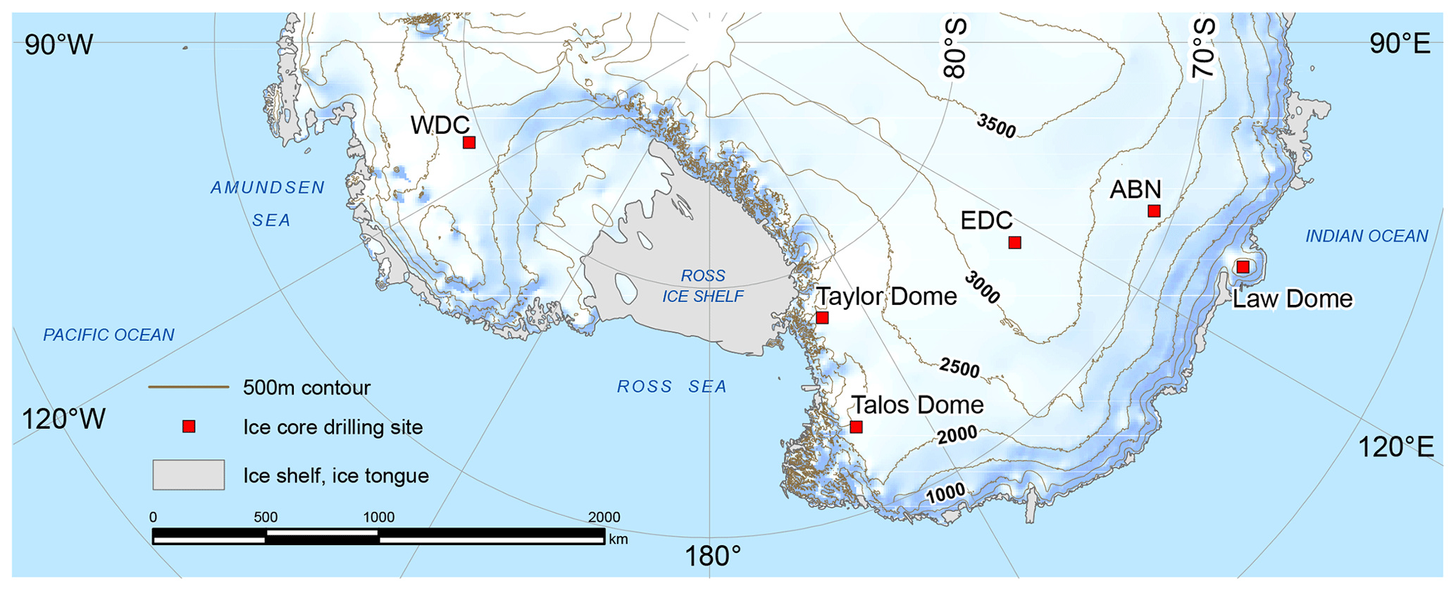
Figure 1Map of the Indian and Pacific sectors of Antarctica. A selection of ice core drilling sites is shown: ABN – Aurora Basin North (this study), Law Dome, EDC – EPICA Dome C, WDC – West Antarctic Ice Sheet Divide Core, Talos Dome, Taylor Dome. True scale at 71∘ S. Modified from a production of the Australian Antarctic Data Centre, June 2009 (map catalogue no. 13641 – http://data.aad.gov.au/ © Commonwealth of Australia 2009). Creative Commons Attribution 4.0 Unported License.
2.2 Measurements
2.2.1 Water stable isotopes
The ABN1314 core was subsampled at 20 cm resolution for water stable isotope analysis at the Australian Antarctic Division. Water stable isotope (noted δ18O and δD, as in IAEA, 1995) analyses were performed on a Picarro L2130-i isotopic water analyser. Aliquots of water were sampled by a Picarro liquid auto-sampler, injected into a Picarro high-precision vaporization module (A0211), and held at temperature of 110 ∘C; then vapour is sent to the Picarro L2130-i isotopic water analyser. Isotopic values are expressed as per mill (‰) and relative to the Vienna Standard Mean Oceanic Water (V-SMOW) standard. The standard deviation of the δ18O values for repeated measurements of laboratory reference water samples was less than 0.05 ‰ and less than 0.5 ‰ for δD. A total of 1522 measurements were performed on the 303 m core. Although δ18O and δD are roughly proportional, deviation from the standard meteoric water line likely results from changes in the evaporation conditions at the moisture source (Dansgaard, 1964; Uemura et al., 2008). The deviation from the meteoric water line can be defined with a logarithmic notation (Uemura et al., 2012).
The propagated uncertainty gives an analytical precision for dln of 0.52 ‰.
2.2.2 Gas stable isotopes
Gas-dedicated samples of about 20 cm in length were subsampled approximately every 2 m in the ABN1314 core. Due to the porosity of the ice sheet, gas samples were taken below the lock-in depth, starting at 104 m depth. The samples' outer 5 mm layer of ice was shaved off to prevent contamination by exchange with air during transport and storage, and each sample was split into two duplicates of ∼70 g each.
In order to measure precise argon isotopes, O2 was removed due to isobaric interference between 36Ar and 18O18O. Argon and nitrogen gases were extracted from the ice following the method of Kobashi et al. (2008): the ice was melted in a pre-emptively evacuated bottle, and the gases were released in a processing line with cold traps to remove water vapour and carbon dioxide, as well as a heated copper mesh (500 ∘C) to remove molecular oxygen. The remaining gases are trapped in a collection tube that is cooled with liquid helium. To maximize the efficiency of the traps, the gases were released slowly in the processing line, with the pressure in the collection tube maintained under 50 Pa at all times. Once the entirety of the gases was released into the processing line, the collection continued for about 15 min, until the pressure dropped under Pa, to ensure complete trapping of the gases. The collected gases are left to heat up to room temperature and homogenize in the collection tube overnight, then measured on a dual-inlet mass spectrometer (MAT 253+) against a laboratory standard gas mixture of N2, Ar, and Kr. The MAT 253+ spectrometer was set up so that different isotopes of the same element are measured simultaneously in an arrangement of collection cups dedicated to N2, Ar, or Kr. The standard is calibrated weekly against modern air following the same protocol as the ice sample, from release in the processing line to mass spectrometry.
We use the δ40Ar and δ15N notations for isotopic ratios 40Ar 36Ar and 15N 14N in the sample relative to the isotopic ratios in the free atmosphere (IAEA, 1995). The dual-inlet system that sends gas to the spectrometer switches between the sample and laboratory standard in cycles for robust measurement of the isotopic ratio. Cycles of 11 standard and 10 sample injections were repeated five times with the spectrometer in argon configuration and three times in nitrogen configuration. Additionally, elemental ratios of Ar N2 were measured following the peak-jumping method (Bereiter et al., 2018).
Pressure imbalance and chemical slope corrections were applied to account for the imbalance in the dual-inlet system and the elemental ratios in the sample, first described by Severinghaus et al. (2003; details of the corrections used in this study are given in Appendix A1). In addition to the previously described corrections, it was determined that the spectrometer focus drifted over time, which resulted in a strong variability of both δ40Ar and the value used for the pressure imbalance correction. While the measurements took about 9 months to complete, the pressure imbalance correction value was verified daily, and estimates of the intensity of δ40Ar error resulting from the spectrometer focus were made using the daily value of pressure imbalance correction, which is itself dependent on spectrometer parameters. We thus corrected for the spectrometer drift (details of this correction are given in Appendix A1). This drift correction reduced the pooled standard deviation of δ40Ar in the ice duplicates from 0.028 ‰ to 0.013 ‰. While Kobashi et al. (2008) have reported argon loss during storage of ice for an extended amount of time at a temperature of −20 ∘C, the excellent quality of ice from a recently drilled ice core and the precautions taken during the preparation prevented any notable effect of argon loss during storage on the δ40Ar measured in our samples, attested by the absence of correlation between δ40Ar and δAr N2 within duplicates.
A total of 102 pairs of duplicates were analysed, and this was complemented by three single samples that could not be duplicated because they were taken from ice samples that were too small to be split in two or for which one sample of the duplicate pair was lost due to a leak during processing. Given that ice samples were processed in duplicate and have undergone the same procedure, we evaluate the reproducibility of the method and analysis by comparing duplicate results. The pooled standard deviation of the 102 duplicates is 0.0159 ‰ for δ40Ar and 0.0045 ‰ for δ15N. Three samples had exceptionally high duplicate differences, with higher than 3 times the pooled standard deviation for either δ40Ar or δ15N. These samples had been flagged as potentially contaminated due to a change of operator and an unplanned power outage during processing. Another four shallow duplicates, taken just below the close-off depth, had δ40Ar and δ15N values significantly lower than the gases in the open porosity of the lock-in depth above. At ABN, the close-off depth of ∼104 m below the surface is where the pores are completely closed, and the air bubbles are trapped in an ice matrix. Recent bubbles in the ice around this depth were probably enclosed by a thin ice wall at the time of sampling and may have been contaminated with more recent air before the pores were fully sealed. Another possibility is that vacuum pumping on thinly closed pores may have altered the isotopic composition during gas sample preparation. These samples were considered outliers and will not be included in the final dataset, which consists of 95 duplicates and three singletons. After removal of outliers, the pooled standard deviation of remaining samples is 0.0137 ‰ for δ40Ar and 0.0036 ‰ for δ15N.
In this article we rely on mass-independent fractionation and thus use (Kobashi et al., 2008; further description will be given in Sect. 3.2). Vertical heterogeneities in firn density of the order of 10 cm (Hörhold et al., 2011) can lead to differences in bubble closure rate with a size-dependent fractionation (Severinghaus and Battle, 2006) and consequently imprint a high-frequency non-climatic signal in 15Nexcess (Kobashi et al., 2015). To reduce the noise induced by pore closure, we average samples in 5 m windows to include samples from at least two distinct depths. The data are thus smoothed by averaging on 5 m windows to average both δ15N and δ40Ar (Fig. 2). The uncertainty in the averaged points was inferred as the standard deviation of all points in the 5 m window. Hereafter in this study, the smoothed data with a 5 m resolution are used.
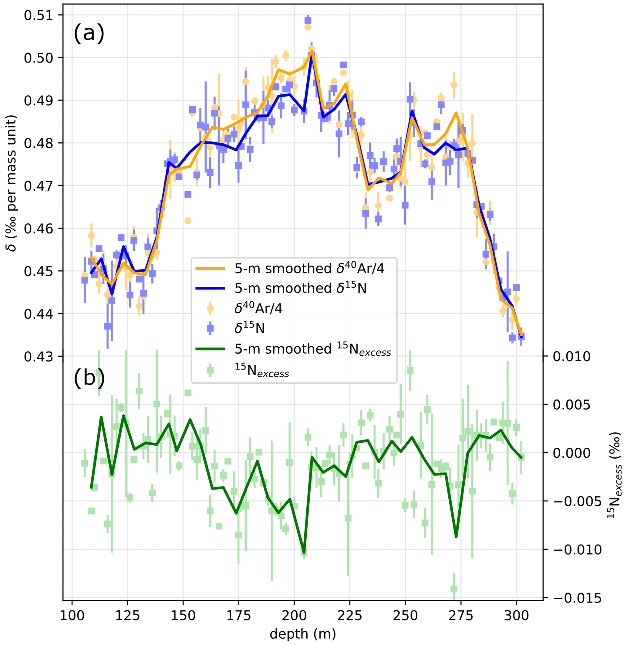
Figure 2Series of δ40Ar (orange), δ15N (blue), and 15Nexcess (green) in the ABN1314 core. Large dots and squares represent the average value for a given depth, and error bars illustrate the difference between duplicates. The 5 m smoothing is shown with solid lines for all series.
2.2.3 Borehole temperature
The borehole temperature measurements were made by lowering a measuring resistor with a three-bladed probe down the borehole. The resistance was measured using a Fluke multimeter and converted to temperature using temperature dependence of resistivity. The probe was left to equilibrate at each depth interval such that the read-out was verified as unchanging. This was achieved within a few minutes and then left to equilibrate an additional 3 to 5 min to ensure a stable value. A second series of measurements was made at the same depths when the probe was pulled back up, providing two temperature values for each depth (downward and upward, Fig. 3). The temperature disturbance at ∼100 m depth is attributable to the addition of drilling fluid (Estisol) stored at the surface into the drill hole, with the last addition just a few days before temperature profiling. Open markers in Fig. 3 will be considered outliers for this reason. Relatively short equilibrium time before each measurement may have caused the downward temperature to be overestimated, whilst the upward temperature series is underestimated because of the memory effect of the temperature probe, particularly above the drilling fluid. Even though the temperature was measured only a few weeks after the drilling had been completed, the heating effect of the drilling is relatively small, estimated at ∼0.1 ∘C (Orsi et al., 2017). The temperature measured ranged from −45.5 ∘C at the bottom of the drill hole to −43.1 ∘C at 17 m below the surface, deep enough for the temperature not to be affected by seasonal variations, revealing a gradient larger than 2 ∘C over the 300 m depth.
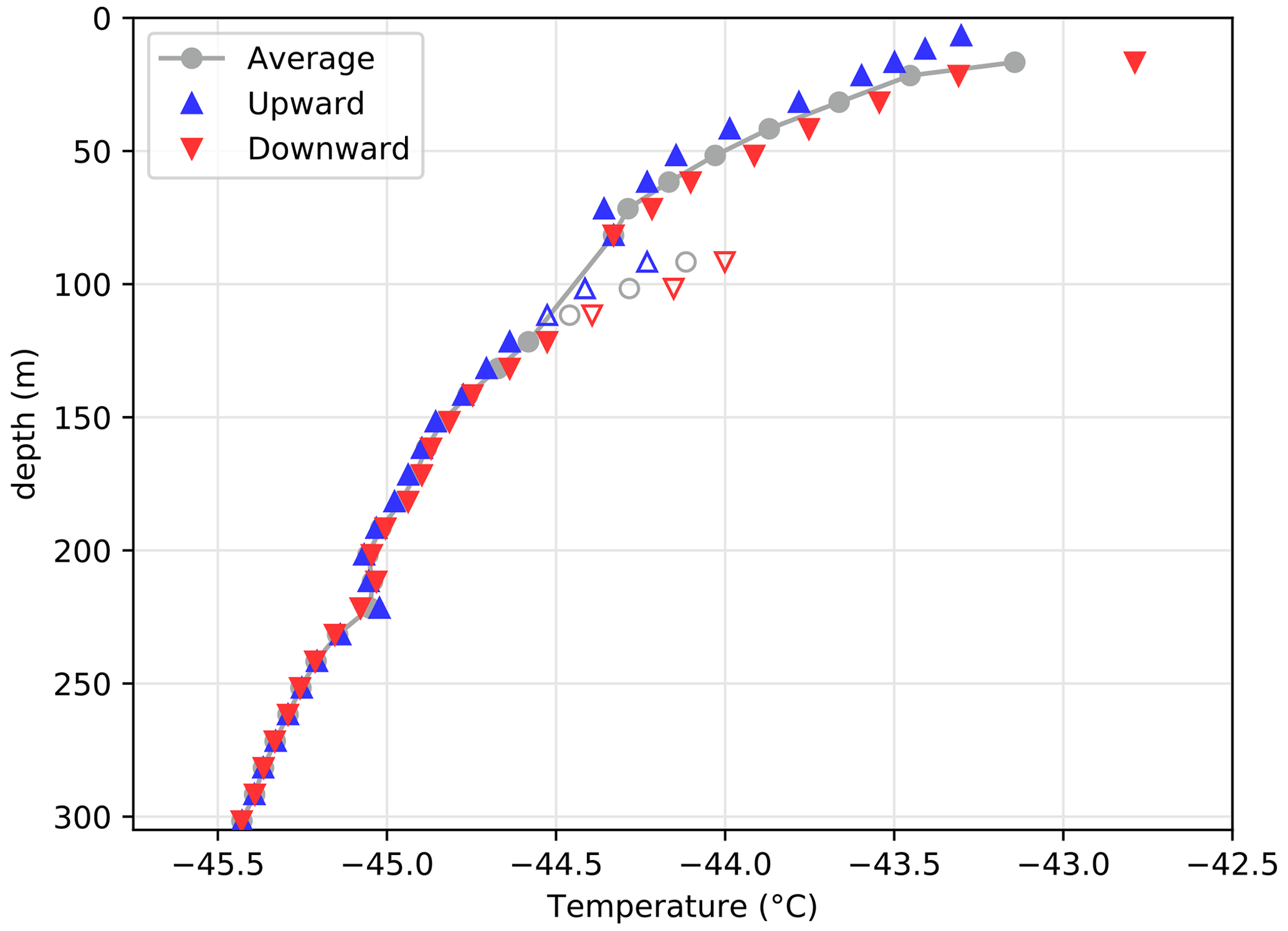
Figure 3Temperature profile in the Aurora Basin North main core borehole. The drilling fluid may have induced a disturbance of air temperature in the drill hole because the drilling fluid was stored at the surface at a warmer temperature of about −20 ∘C. Open markers indicate points that will be ignored for this reason. Below 132 m, the small difference between upward and downward measurements is likely due to improved equilibrium in the drilling fluid.
2.3 Ice core age model
2.3.1 Ice age model
Producing a well-constrained age model is a necessary step in the analysis of a paleoclimate record. Chemical species, electro-conductivity, and water stable isotopes were measured at high resolution with continuous flow analysis (CFA) at the Desert Research Institute (Maselli et al., 2013; McConnell et al., 2002) and allowed identification of annual cycles in most of the ABN1314 ice core. The ABN1314 core was dated by annual layer counting (ALC) of seasonally varying aerosols (Na+, Cl), electro-conductivity, and water isotope measurements. Although water isotopes are also measured on the CFA system, the CFA data were only used to build the age model; in this article we discuss the isotope data from discrete sampling measured at the Australian Antarctic Division (Sect. 2.2.1). The ALC was performed manually and subsequently tied to volcanic events using sulfate aerosols from other well-dated ice core records. The ABN1314 total sulfur record was compared to the Plateau Remote (Cole-Dai et al., 2000) and West Antarctic Ice Sheet Divide (Sigl et al., 2013) ice cores, as all sites are in inland Antarctica and have similar backgrounds for sulfur. Even though Law Dome is the nearest site with a high-resolution sulfur record, the background is very different, likely due to Law Dome being a coastal site. ALC was adjusted using 29 volcanic horizons that were matched to the WD2014 chronology (Sigl et al., 2016). The surface snow mixing by wind at ABN is of comparable scale with the yearly accumulation (up to 40 cm of snow, Servettaz et al., 2020), which may have hindered the identification of annual signals used for year identification in ALC, especially during periods of lower accumulation. Therefore, the ABN1314 ALC was anchored to the WD2014 chronology with volcanic ties, and then ALC was performed a second time between ties to find the expected number of years. The uncertainty in the age of volcanic horizons in the WD2014 chronology is lower than 5 years, and hence we report all the volcanic ties with a ±5-year margin to account for this uncertainty.
The ABN1314 core covers the last 2700 years (Fig. 4). Dating uncertainties resulting from the ALC were considered as follows: if an annual layer was counted but is not on a clear seasonal peak, it is flagged as uncertain, and a half-year uncertainty is added (details on the uncertainty are shown in Fig. A8). The age model for the ABN1314 core is referred to as ALC-01-11-2018. Through the volcanic age tying, the age model for ABN1314 has consistently low uncertainties of less than 20 years.
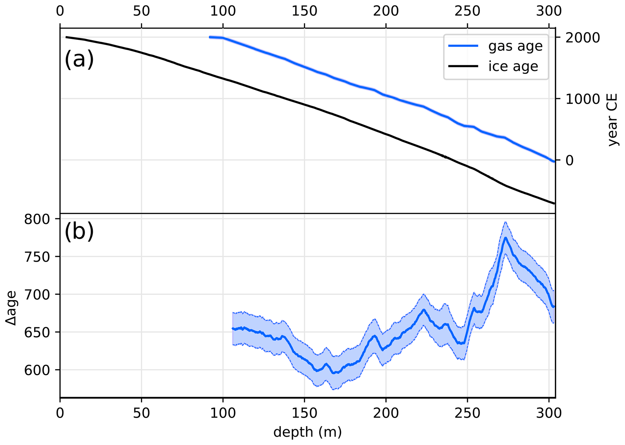
Figure 4(a) Ice and gas age models for the ABN1314 ice core. The ice age model is based on annual layer counting of seasonally varying chemical species, while the gas age model is based on methane ties. Both age models are tied to the WD2014 chronology for ice and gases, respectively (Sigl et al., 2015, 2016). (b) The Δage is defined as the difference between ice and gas ages at each corresponding depth. Shading indicates the estimated uncertainty.
2.3.2 Gas age model
The gases are trapped by closure of the porosity at the bottom of the firn, and hence are enclosed in bubbles surrounded by substantially older ice. Preliminary dating of the gases is completed by subtracting a constant age difference to the surrounding ice, corresponding to the modern-day difference between age of gases and ice at the lock-in depth. Firn characteristics may vary through time, affecting the height of the diffusive zone and thus the lock-in depth, and hence the gas age model is further refined with the methane record measured in the ABN1314 core.
The methane content of gases trapped in ABN1314 was measured with the Desert Research Institute continuous flow analysis system that was modified for gas measurement (Rhodes et al., 2013). We used methane records to tie the gas age scale of the ABN1314 core to the established chronology of the WAIS Divide ice core, named WD2014 (Sigl et al., 2016). Specifically, we defined tied points so that the methane content in bubbles at ABN fits the published methane dataset from the West Antarctic Ice Sheet (WAIS) Divide ice core, named WD2014 (Sigl et al., 2016). A total of 14 tie points were identified where there are clear, quick transitions or extrema in methane records (Fig. A9). For the most recent part (1800 to 2000 CE, Fig. 4b), the methane data from WAIS Divide were not available, and hence the ABN methane record was tied to the revised Law Dome record (Rubino et al., 2019) with four additional tie points. Again, samples taken above the close-off depth of ∼104 m below the surface, which corresponds to 1925 CE, are likely to be contaminated with recent air before the pores were sealed, resulting in higher methane concentrations.
The gases are younger than the ice at the same depth, so the gas age model of ABN1314 core only covers the last 2050 years (Fig. 4). The most recent gases are technically still in the diffusive column of the firn, or partly in the remaining open porosity between lock-in and close-off depth, but not fully trapped in bubbles within an ice matrix. The uppermost ice core samples that contain gases suited for analyses are found below the close-off depth, dated to 1925 CE. Because the ages were tied manually, it is difficult to estimate the uncertainty, but the tie points used correspond to events with an age span shorter than 20 years. While the lock-in depth of gases may vary depending on the species due to diffusivity speed in the firn (Witrant et al., 2012), the resulting difference is expected to be much lower than 20 years at ABN. Therefore, we roughly estimate the uncertainty in the gas age model to be 20 years.
2.3.3 Gas–ice age difference
The difference between gas age and ice age provides information on the dynamics of the firn and its evolution through time. A larger age difference may result from a decrease in accumulation rate or an increase in lock-in depth where gases are trapped. The gas–ice age difference at a given depth (Fig. 4b) is comprised between 600 and 700 years, except for one excursion at around 270 m depth which is likely related to the sudden change in accumulation caused by a dune-like feature upstream from the ABN site, which was advected under the current ABN location with ice flow.
2.4 Ice flow correction
In opposition to many ice core drill sites that target a dome or a divide, the ABN1314 ice core was drilled in a basin setting, where ice slowly flows from the continent to the coast. The estimated ice flow is determined by comparing the accumulation record from the ice age model and the first isochron reflector depth from the ground-penetrating radar survey upstream of ABN: the first order of accumulation changes is driven by local accumulation features caused by the topographic slope (Van Liefferinge et al., 2021; Akers et al., 2022). Indeed, the speed of the katabatic wind scales with terrain slope (Parish and Bromwich, 1991; Vihma et al., 2011), and thus acceleration of wind scales with terrain curvature. Accelerating winds can charge up in snow particles and locally reduce the accumulation. Conversely, decelerating winds deposit the drifting snow, increasing the accumulation. By matching the time series of accumulation from the ABN1314 core to the upstream accumulation patterns (Fig. A10), we estimate that the bottom part of the ABN ice core corresponds to ice originating 41.5 km upstream from the ABN drill site, which results in an average ice flow of 15.4 m yr−1. This value is in relatively good agreement with satellite-based estimation of 16.2 m yr−1 at ABN for the 1996–2018 period (Mouginot et al., 2019).
Using this ice flow velocity, the estimated origin altitude of the ice in the ABN1314 core, or the paleo-elevation of the ABN drilling site, is made. The ice dating from 700 BCE was deposited at an elevation of 2745 m, and subsequent ice forming the ABN1314 ice core originated from lower elevation, down to the drill site at 2690 m for the most recent snow (Fig. A10). We estimated that a decrease of 55 m elevation would cause a temperature increase of 1 ∘C using the temperatures interpolated with kriging from automatic weather stations and borehole temperature measurements for two traverses in nearby Princess Elizabeth Land, East Antarctica (Xiao et al., 2013; Pang et al., 2015; Fig. A11). The regression was performed on a subset of the traverse between 2000 and 3250 m above sea level, corresponding to the lower plateau around the elevation where ABN is located. Similarly for water stable isotopes, the estimated decrease of 55 m elevation would result in a δ18O increase of about 1 ‰ by calibrating a δ18O–elevation slope in surface snow studies at elevations between 2000 and 3250 m above sea level and longitudes from 80 to 160∘ E (Xiao et al., 2013; Pang et al., 2015; Goursaud et al., 2018; Fig. A12). The measured δ18O and ice-flow-corrected δ18O are shown in Fig. 5. We did not find any significant relationship between elevation and dln at this elevation range (Fig. A13) and therefore did not correct it for glacial flow.
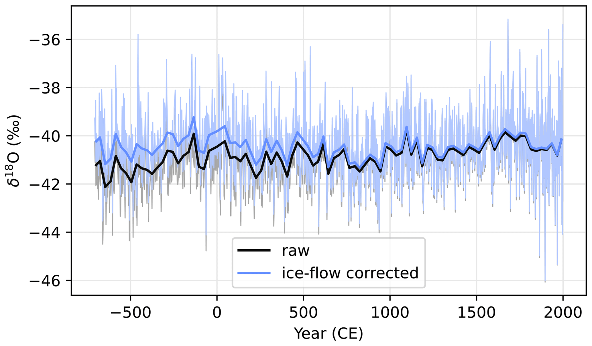
Figure 5δ18O in the ABN1314 ice core, with a sampling resolution of 20 cm (thin lines) and on 30-year average (Thick lines). The analytical uncertainties in δ18O of 0.5 ‰ are not shown in the figure. Black lines show the raw measurement, and blue lines show the glaciology-corrected values.
3.1 Water stable isotopes
Water isotopes in ice cores have consistently been used to estimate past temperatures (e.g. Cuffey et al., 1995; Jouzel et al., 1997, 2003; Stenni et al., 2017). The ABN isotope record consists of 1522 data points for the 2707 years covered by the ice core, resulting in a temporal resolution of δ18O slightly above one point for 2 years. However, the water isotopes are strongly affected by deposition variability and non-climatic factors that may mask the climate signal at high resolution, especially for regions such as the East Antarctic plateau where the accumulation is low (Münch and Laepple, 2018; Casado et al., 2020). Moreover, a few extreme precipitation events can be responsible for a large part of the total yearly accumulation (Turner et al., 2019), so it is more reliable to average over several years to retrieve the climate information from the water isotope record. Therefore, a 30-year average is used to better determine the climate signal. The 30-year averaged δ18O series has a mean value of ‰ (1σ) and shows minimal variation over time.
We chose to determine the ABN δ18O–temperature slope using the δ18O record from the 12 m shallow core described in Servettaz et al. (2020) and temperatures from the regional atmospheric climate model MAR (Modèle Atmosphérique Régional, available at https://gitlab.com/Mar-Group/MARv3, last access: May 2023; we use a simulation described in Agosta et al., 2019) nudged to ERA-Interim climate reanalysis (Dee et al., 2011). The MAR model was developed with implementation of specific physical parameterizations for polar regions, with a turbulent scheme adapted for stable conditions of the Antarctic plateau. It has a high vertical resolution with five levels within the first 10 m, which enables a good representation of temperature inversion. Consequently, MAR was shown to model the surface temperature more accurately than any other available dataset when compared with automatic weather station observations at GC41 (48 km south of ABN), with a bias lower than 1 ∘C (Servettaz et al., 2020). Water stable isotopes in the shallow core were measured at high resolution with continuous flow analysis (CFA) at the Desert Research Institute (Servettaz et al., 2020). The shallow core is dated back to 1968 and overlaps with the MAR modelled temperature for the 1979−2013 period, although annual layers could only be identified down to the Pinatubo eruption (1991). Below this depth, uncertainties in the dating do not allow for clear annual averages, and multi-year average could lessen the range of variability. Therefore, we calibrate a δ18O–temperature slope for ABN using linear regression on the 1991 to 2013 period. Both temperature and δ18O are averaged annually to minimize the influence of seasonal variability.
We determine a δ18O–temperature slope α=2.01 ‰ ∘C−1, with a 95 % confidence interval of 1.16 < α < 2.87 ‰ ∘C−1. According to this slope, a change of 1 ∘C in the mean annual temperature would be recorded in the snow by a ∼2 ‰ change in δ18O. This 2.01 ‰ ∘C−1 slope is relatively high compared with other slope values estimated with ECHAM5-wiso, which average 1.00 ‰ ∘C−1 in East Antarctica (Stenni et al., 2017) or 0.85 ‰ ∘C−1 at ABN (Servettaz et al., 2020). This difference could be at least partly attributed to the ECHAM5-wiso model, known to underestimate the inter-annual variability of isotopes in Antarctica (Goursaud et al., 2018).
Here, we use the 2.01 ‰ ∘C−1 slope to convert the δ18O corrected for ice flow from ABN1314 to a reconstructed temperature record (Fig. 6c). The ice flow correction described in Sect. 2.4 is applied to the δ18O data before converting it to a temperature record to emulate a δ18O record at the current ABN location. The δ18O–temperature calibration slope was defined on a shorter period of 23 years that should not be affected by ice flow. The temperature obtained from this reconstruction averages −42.0 ∘C and remained within a 1 ∘C range (from −42.6 to −41.6 ∘C) over the past 2700 years (Fig. 6). The use of a different δ18O–temperature slope slightly modifies the range of temperature values (Fig. 6c) but does not modify our interpretation. We acknowledge that using a δ18O–temperature slope calibrated with yearly averages is not optimal given the limitations caused by deposition dynamics and post-deposition processes, but the δ18O–temperature calibration is limited by the length of overlapping δ18O and available temperature records. The temperature reconstruction from δ18O at ABN might also be biased, as precipitation consistently occurs during warm events (Servettaz et al., 2020).
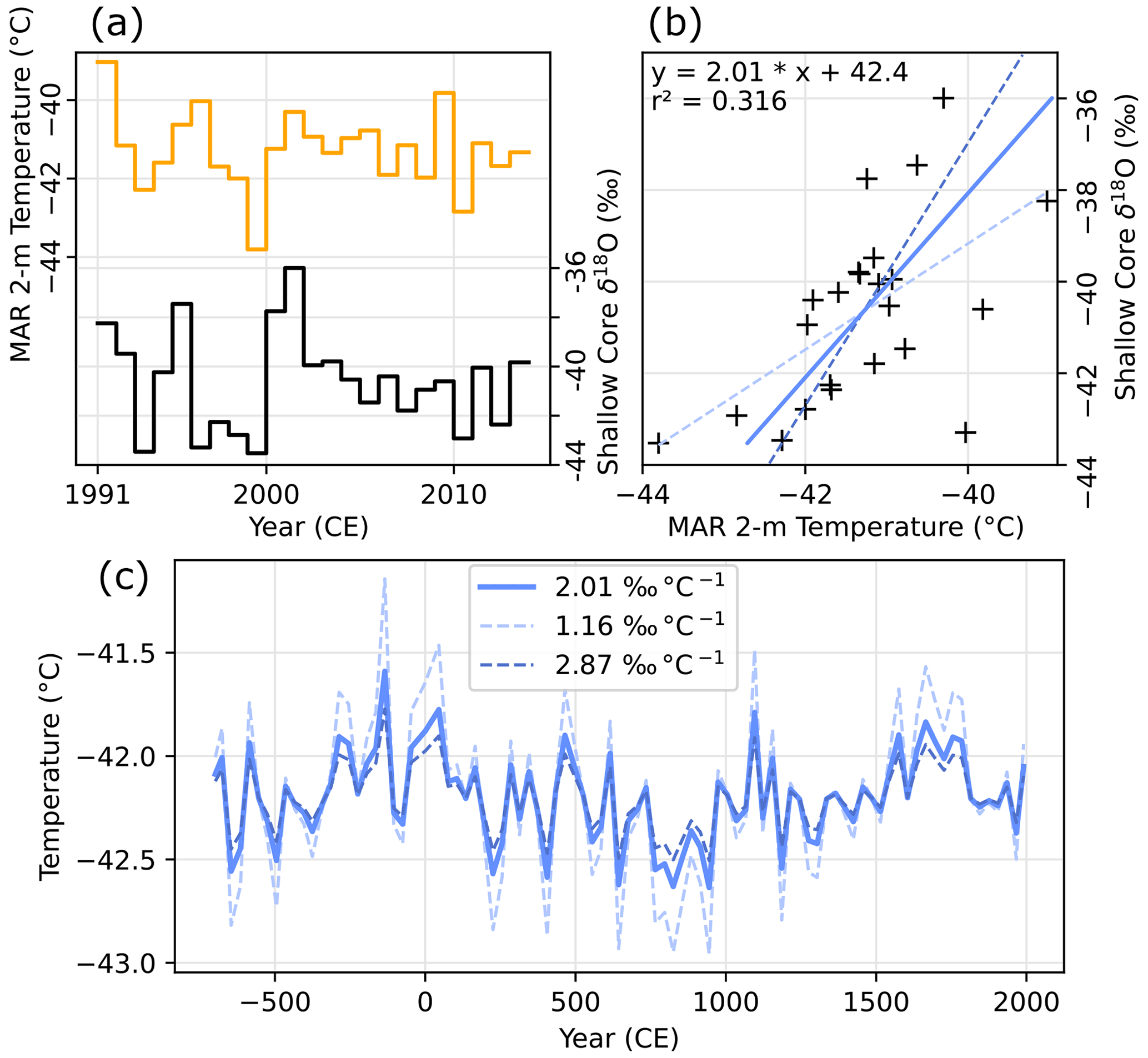
Figure 6Calibration of the δ18O–temperature slope with the Desert Research Institute shallow core δ18O and the 2 m temperature in the Modèle Atmosphérique Régional (MAR) on the 1991–2013 CE period. (a) Annually averaged series of MAR 2 m temperature (orange) and shallow core δ18O on the 1991–2013 period. (b) Scatter plot of the two datasets (black crosses), with linear regression shown as a blue solid line. Dashed lines represent the slope upper and lower uncertainties at a 95 % confidence level. (c) Temperature reconstruction using the δ18O series from the ABN1314 core and the slope obtained with linear regression, with temperature reconstructed with upper and lower uncertainty slope values shown as dashed lines.
3.2 Gas and borehole temperature inversion
While water isotopes have been the proxy of choice for many paleoclimate studies in Antarctica, past temperatures are also imprinted in the ice and can be measured in the borehole after the ice core has been drilled. However, the temperature slowly diffuses in the ice, smoothing out the signal over time. Diverse inversion methods have been applied to estimate temperature changes since the last deglaciation (e.g. Dahl-Jensen et al., 1998) or over the last millennium (Orsi et al., 2012), but the temperature reconstruction from a borehole quickly loses temporal resolution over time. Another method to estimate past temperature changes relies on the thermal fractionation of gases in the firn diffusive column, where a gradient of temperature can be captured in the δ15N and δ40Ar composition of the air trapped in bubbles of the ice core (Kobashi et al., 2008; Orsi et al., 2014). Here, we also reconstruct past temperatures at ABN using a combination of the borehole temperature and the past temperature gradients estimated from gas isotopes.
3.2.1 Determination of temperature profile and past temperature gradients
The temperature profile was measured directly in the borehole after the ice core was drilled. The temperature profile of the ABN borehole (Fig. 3) shows a strong decrease in temperature at depth, suggesting that the surface warmed while old ice buried under remained colder. We observe a near-surface temperature gradient of ∼1 ∘ C 100 m−1, for which a 2.7 ∘C warming over the last 30 years was inferred at a Greenland site (Orsi et al., 2017). On the East Antarctic plateau, however, no such warming trend was previously detected (Nicolas and Bromwich, 2014). We expect that the ABN temperature gradient partly results from ice rheology, displacing the ice from a colder location upstream to what is now buried under the ABN site.
Gravitational fractionation and thermal fractionation affect the gas contained in the firn porosity. The temperature gradient in the diffusive column controls the thermal fractionation, while the height of the diffusive column determines the gravitational fractionation. Knowing the fractionation coefficients, we retrieve the temperature gradient (noted ΔT) of the firn at different times. The gravitational effect on isotopes (noted δgrav) is mass-dependent, while the thermal fractionation can be approximated as a linear function of the temperature gradient in the firn, with different fractionation coefficients for nitrogen (Ω15) and argon (Ω40) gases (Severinghaus et al., 2001). Gravitational and thermal effects on fractionation can thus be disentangled using two pair of isotopes, as described by the following system.
So δgrav and ΔT can be written as a function of δ15N and δ40Ar.
We use Eq. (3) to estimate the temperature gradient and gravitational fractionation from the gas isotopes. We use values of 0.0143 ‰ ∘C−1 for Ω15 and 0.0386 ‰ ∘C−1 for Ω40 at 229.5 K or −43.7 ∘C (Grachev and Severinghaus, 2003). The diffusive column height is calculated from gravitational fractionation using the following equation (simplified from Sowers et al., 1992):
where R is the gas constant, T is the temperature, and g is the gravitational acceleration. We used a constant temperature of 229.5 K (−43.7 ∘C), derived from the borehole temperature measurement at 20 m depth in the ABN firn, where season variations do not reach. The average uncertainty for the δgrav is 0.008 ‰, resulting in a 1.5 m uncertainty in the diffusive column height (zdiffusive). A pooled standard deviation of 15Nexcess in the ice samples gives an analytical uncertainty of 0.0027 ‰, resulting in a ΔT uncertainty of 0.3 ∘C. Sample preparation includes release of gases in empty lines and can induce a pressure gradient leading to small fractionation in both δ15N and δ40Ar, which is apparently mass-dependent (Severinghaus and Battle, 2006). In the definition of 15Nexcess, mass-dependent processes are cancelled out, and therefore the difference in 15Nexcess between the two samples is smaller than δ15N or δ40Ar alone (0.0137 ‰ for δ40Ar and 0.0036 ‰ for δ15N).
The temperature difference (ΔT) reconstructed from gases is representative of the gradient between the surface and the lock-in depth. The lock-in depth can be deeper than the diffusive column height in the case of near-surface convective mixing. Therefore, we also estimate the lock-in depth with the gas–ice depth difference at the same age from the age models (Sect. 2.3, Fig. 4). The gas–ice depth difference decreases over time because of the compaction in the firn and ice column, so we deconvolve the depth difference using a mass-conservative compaction model fitted to the modern profile of snow and ice density measured in the ABN1314 ice core.
In short, we compute the mass of ice between the depth of gases and ice of the same age, and we find the modern depth where the overlying total ice mass up to the surface is identical. In this model, we assume that the density profile remains the same over time. This estimation of the past lock-in depth is called the deconvoluted Δdepthice-gas. Given the ∼20-year uncertainty in the age difference, the deconvoluted Δdepthice-gas has an uncertainty of ±3.8 m.
Evolutions of the ΔT, deconvoluted Δdepthice-gas, and diffusive column height are shown in Fig. 7. We define the true lock-in depth (Fig. 7b) as the deepest diffusive column height and deconvoluted Δdepthice-gas because the lock-in depth can be deeper than diffusive column height in the presence of a convective zone, but the lock-in depth should be at least as deep as the diffusive column height. The points where deconvoluted Δdepthice-gas (dashed line) is shallower than the diffusive column height are within the 3.8 m uncertainty. They may result from errors in the age model or in the compaction model: a less-dense than modern profile would yield greater ice–gas depth differences in better agreement with the diffusive column height. However, improved precision is not required in this study, as errors of ±3.8 m in the lock-in depth result in ±0.03 ∘C in the surface to lock-in depth temperature gradient, 10 times smaller than the uncertainties in the ΔT estimated from the gas isotopes. Changes in the firn depth (lock-in depth) are most likely driven by changes in accumulation (Sowers et al., 1992; Goujon et al., 2003), which is itself strongly dependent on ice flow and changes in the local slope (Akers et al., 2022; Fig. A10). The main forcing for the lock-in depth is thus not a temperature factor, and we will simply use the value to compute the temperature gradient in the ice sheet (ΔT between the surface and lock-in depth).
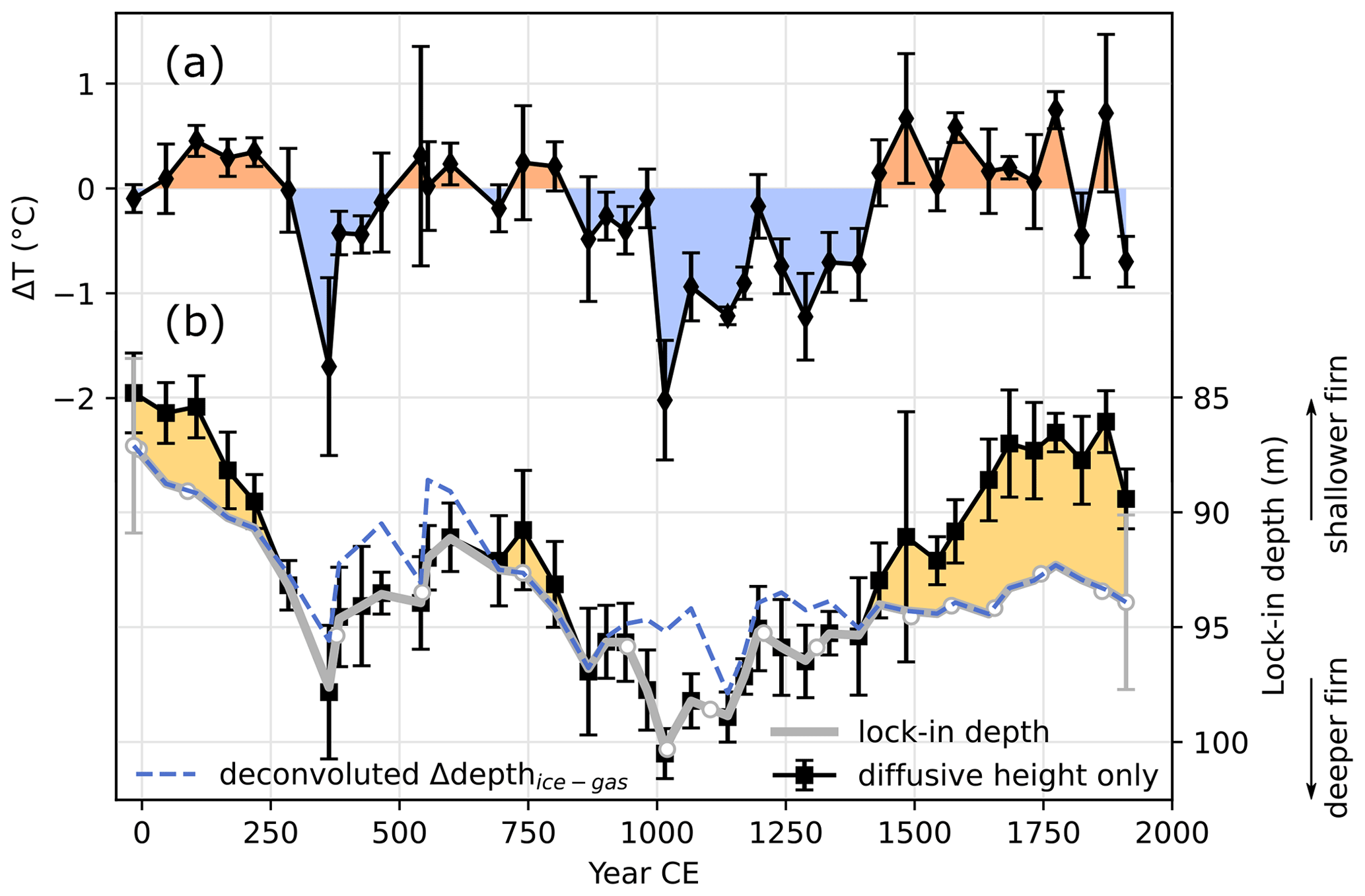
Figure 7(a) Series of ΔT computed from 15Nexcess. Orange shading indicates a warming (ΔT > 0) and blue shading a cooling (ΔT < 0). (b) Past lock-in depth (thick grey line) estimated from diffusive column height of gas isotopes (black line with error bars) and gas–ice depth difference (blue dashed line). Yellow shading highlights the potential presence of a convection zone that would be located in the uppermost layer of the firn (0–5 m depth) when the lock-in depth appears to be deeper than the diffusive column height. For clarity, uncertainties in the lock-in depth are only shown at both ends of the record. White dots on the lock-in depth indicate the ages at which the gas age model was tied to WD2014, indicating the constraints on the Δdepth. The y axis for the firn column depth was flipped so that deeper lock-in depths are represented as lower points.
3.2.2 Firn temperature diffusion modelling and inversion
We use an ice advection and densification model with temperature diffusion in the ice column to simulate the evolution of the firn under different temperature scenarios. This model has been previously described in Orsi et al. (2012) and we use the parameters described in the Appendix A4. Briefly, this model uses a prescribed series of surface temperature, snow accumulation, and bottom geothermal flux to simulate the evolution of temperature in the firn and ice column. In our simulations, densification follows the modern density measurements, and the lock-in depth is inferred from the depth determined previously with deconvoluted Δdepthice-gas and diffusive column height. We create 220 temperature simulations by adding a small perturbation ramping up to +1 ∘C on 10 years to a base temperature history estimated from Dome C (Jouzel et al., 2007) and ice-flow-related temperature changes (Mouginot et al., 2019; details of the temperature forcings are in Fig. A14 and Appendix A4).
We find the optimized temperature history that fits both the present-day borehole temperature profile and the past ΔT temperature gradients estimated from the 15Nexcess. The optimized temperature history is estimated by least square regression of a linear combination of the 220 temperature simulations to the borehole temperature profile (e.g. Orsi et al., 2012) and the temperature gradients estimated with 15Nexcess (e.g. Orsi et al., 2014). In this study, we use both borehole and gas data to constrain the temperature history; the borehole temperature profile constrains the long-term changes, while the 15Nexcess constrains temperature changes at the scale of ∼ 20 to ∼ 200 years (the diffusion time in the firn column of gases and temperature, respectively). However, the two datasets result in a mismatch for the long-term trends, with 15Nexcess suggesting a cooling trend. To reconcile the 15Nexcess with the borehole temperature profile, a correction of +0.0046 ‰ is applied to 15Nexcess: this minimizes the standard deviation of the temperature reconstruction as it tries to squeeze in rapid temperature changes to arrange for diverging datasets if 15Nexcess is left uncorrected (Figs. A16 and A17). This 15Nexcess correction for ice samples could be related to expulsion of gases through ice matrix during bubble formation in the firn-to-ice transition (Severinghaus and Battle, 2006), although the effect on 15Nexcess has never been clearly quantified (Kobashi et al., 2015). We apply the same correction to all points because it results from physical processes during the formation of bubbles, and we consider it to remain constant at the timescales studied here. A similar correction of +0.0037 ‰ has been used at WAIS Divide (Orsi, 2013) based on the mismatch between firn air and shallow ice measurements. This correction implies that the long-term trend is constrained by borehole temperature rather than 15Nexcess absolute values. Further work in the firn-to-ice transition is needed to better quantify the effect of bubble formation on gas isotopic composition.
Ice flow is expected to affect the temperature profile in the ice at ABN because it advects ice from a location further upstream that was colder when the snow deposited. This can explain the presence of cold ice at depth under ABN, which could be misinterpreted by the inversion as a climatic warming trend. To account for this effect, we consider the ice in the diffusion–advection model in a Lagrangian perspective and dissociate temperature changes caused by site displacement from climatic temperature changes (details and justifications are given in Appendix A4). After inversion of the model, the ice-flow-related temperature change is subtracted in order to retrieve the climatic temperature changes (Fig. 8). This relies on the assumption that ice flow is in a steady state and the spatial temperature gradient remained constant over the past 2000 years during which we present our temperature reconstruction.
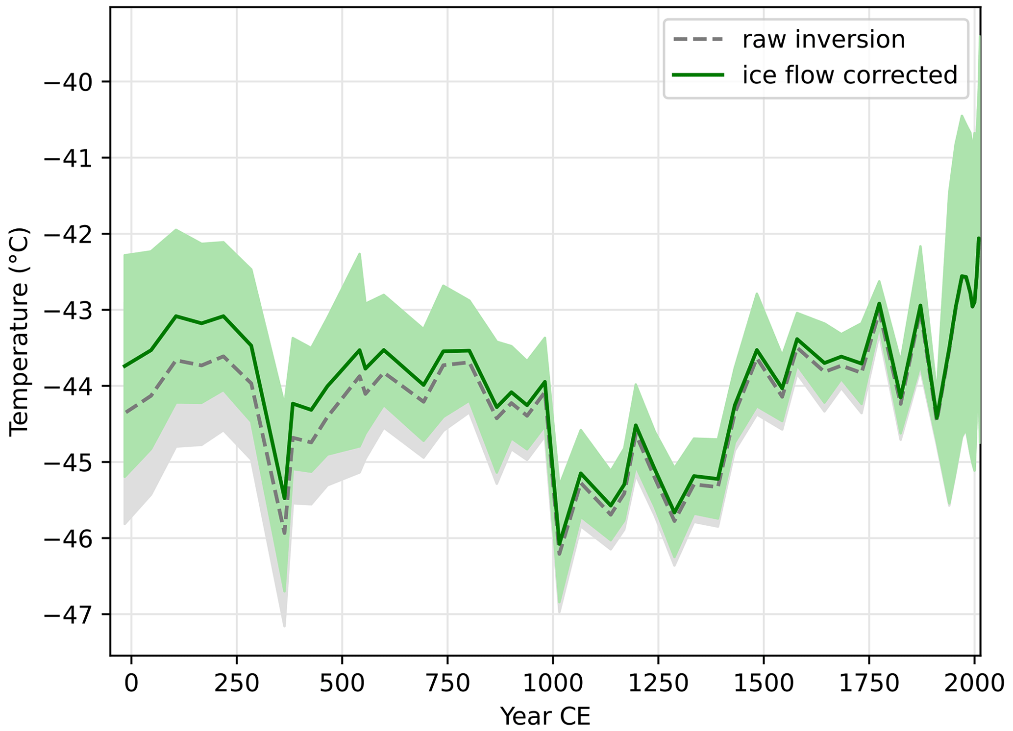
Figure 8Temperature history reconstructed from the 15Nexcess and borehole temperature inversion. The grey dashed line shows the raw inversion, and the green line shows the glaciology-corrected values. The shading represents errors estimated from the inversion, which depend on measurement precision.
Uncertainties of the diffusion model inversion are calculated following the method described by Orsi et al. (2014), where uncertainty of model parameters is scaled to the uncertainty in ΔT and borehole temperature data used for the inversion. A smoothing parameter is used to constrain the inversion by limiting the degree of variability of two temperature simulations with perturbation occurring close together in the linear combination used for the inversion. During the inversion, we use a smoothing parameter to avoid noisy reconstruction with sharp, unrealistic transitions. Temperature points in the inversion are forced into a limited range, determined as an exponentially decreasing tie to neighbour points so that two points at a time difference of 70 years have a covariance of 0.5. This window ensures that each point of the inversion is influenced by gas constraints on ΔT, which have an average time resolution of 45 years. Finally, a signal-to-noise ratio parameter is adjusted to force the inversion temperature to fit to the real borehole and ΔT data points within the error, with a minimum cost on the inversion uncertainty (Figs. A18 and A19). The average uncertainty in the temperature reconstruction is ±0.7 ∘C.
4.1 Differences between the reconstructions
The temperature at the ABN ice core site is reconstructed from water stable isotopes (hereafter called δ18O temperature) and from the inversion of the temperature profile in the borehole and past temperature gradients estimated from inert gas stable isotopes (hereafter called 15Nexcess temperature, Fig. 9). The δ18O temperature is relatively constant, supporting stable conditions of about −42 ∘C, with less than 1 ∘C change during the past 2700 years, whereas the 15Nexcess temperature is marked by changes in temperature of an amplitude of 2 to 3 ∘C, with cold periods from 300 to 450 CE and from 1000 to 1400 CE, as well as a recent warming of about 1 ∘C. Although the temperature reconstructions use measurements from the same core, the material used for the reconstructions differs fundamentally, which can explain some of the disparity.
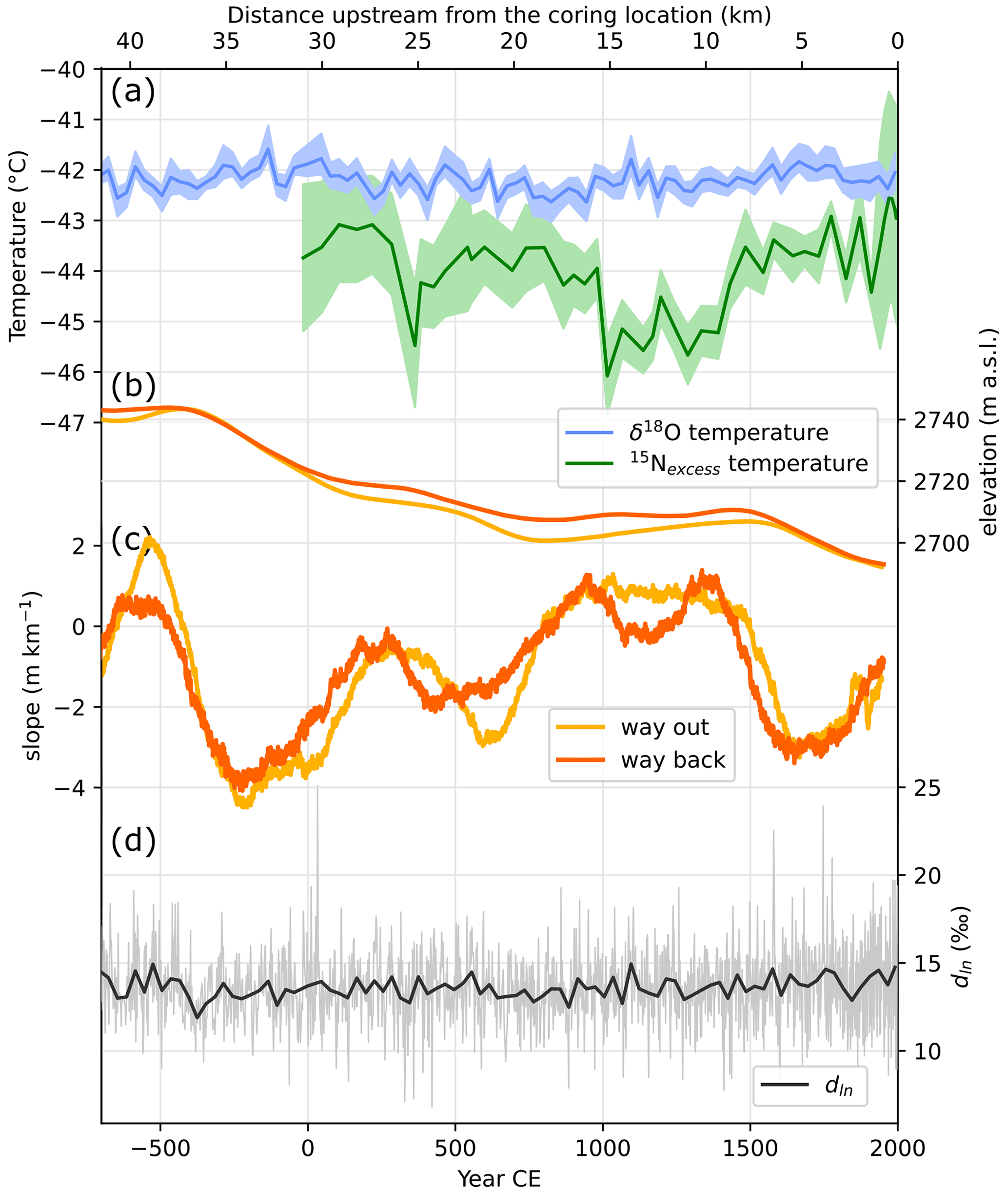
Figure 9Comparison of δ18O temperature and 15Nexcess temperature reconstructions (a) with upstream elevation (b), upstream slopes (c), and dln (d) in the ABN1314 ice core. Distance upstream is indicated on the top axis, and time is indicated on the bottom axis; the correspondence relies on the assumption that the ice flowed at a constant rate of 15.4 m yr−1 (41.5 km in 2700 years). Error shading in (a) represents the error depending on the slope used for the reconstruction from δ18O and the same as in Fig. 8 for 15Nexcess. Elevation was determined with truck GPS position during upstream radar profiling. The profile was taken twice: moving away from the coring site (way out) and going back to the coring site (way back). Original GPS coordinates were not taken in optimal conditions (moving truck), hence the uncertainty.
First, regarding the time significance, water isotopes in ice are accumulated intermittently during precipitation events, while gases are continuously available, and the temperature permanently diffuses in the ice. The sporadic nature of precipitation and the consistent warm anomaly associated with precipitation at ABN may cause water isotopes to inaccurately represent the mean temperature (Servettaz et al., 2020). In particular, the cold and dry conditions that can occur on the East Antarctic plateau are likely to be under-represented in the water isotopes because a large part of the snow accumulation can be attributed to a few precipitation events (Turner et al., 2019). This may cause the δ18O temperature to misrepresent the on-average colder periods if they are still interrupted by less frequent but similarly warm precipitation events or if the seasonality of precipitation changes with a relatively increased contribution in summer during these cold periods. Additionally, long periods without snow precipitation contribute to increasing the snow δ18O by preferential sublimation of light isotopes (Hughes et al., 2021), smoothing out the signature of cold periods. Here, the precipitation events continue to carry the water isotopes with a constant signature of −42 ∘C. On the other hand, due to the slow diffusion of gases in the firn, the signal integrates temperature variation over a time window of a few decades (Witrant et al., 2012; discussed in Appendix A5), but effectively records the temperature even if there are changes in the accumulation regime. Therefore, changes in the seasonality of precipitation with a shift to drier winters could explain both colder conditions in the winter and a lack of snow accumulation, resulting in the failure of water isotopes to capture the cold conditions in the record (Servettaz et al., 2020).
Second, there is a spatial discrepancy between the two reconstructions: the δ18O temperature signal is initially acquired in the atmosphere during the condensation of the precipitation when the condensate phase is exchanging with water vapour (Jouzel and Merlivat, 1984), whereas gases in the firn are in equilibrium with the gradient imposed by snow surface temperature. Changes in the strength of near-surface temperature inversion could drive differences between the two temperature records. Inversion could intensify cooling in the snow during cold periods as the changes are much stronger at the surface level. However, here, the cold periods identified with the gas and borehole temperature reconstruction are not matched by any sign of cooling in the δ18O record, suggesting that the differences are not entirely caused by atmospheric temperature changes amplified by the temperature inversion.
Wind-induced turbulence and mixing can also modulate the inversion strength (Hudson and Brandt, 2005; Pietroni et al., 2014). The average katabatic wind speed increases with the terrain slope (Parish and Waight, 1987; Parish and Bromwich, 1991; Vihma et al., 2011). At ABN, the topographic slope at the source ice location changes over time due to the ice flow (Fig. 9c) and can provide information on slope modulation of katabatic wind speed, although this is the slope along the ice stream flow line and not exactly on the katabatic wind flow line. A reduced slope between 18 and 8 km upstream from the coring location, which is where ice in the ABN core was deposited during the 800 to 1500 CE period, could favour slower winds and a stronger inversion, leading to cooler surface temperature. Nevertheless, linear regression of reconstructed surface temperature and slope at source ice is 0.24 ∘C (m km with a squared Pearson correlation r2 lower than 0.09, which does not support a strong influence of slope on the average surface temperature. At most, the full range of slope variation would explain a difference of 1 ∘C, with low confidence. Furthermore, the recent warming of 1 ∘C cannot be attributed to changes in the slope as the warming occurs while the slope gets gentler. Therefore, we attribute the changes in 15Nexcess to climate factors rather than advection-related changes in slope and wind.
Influence of temperature on δ18O could be masked by a concurrent change in moisture source: e.g. if cold periods were associated with a shift towards a warmer source, the two effects could compensate for each other and result in a constant δ18O. Such a change in moisture source can be recorded in the dln, which efficiently tracks changes in the moisture source temperature (Uemura et al., 2012; Markle and Steig, 2022). The dln series shows no significant trend, with the values averaging 13.6 ‰. When averaged over 30 years to smooth out noise, the standard deviation of dln is only 0.6 ‰, with no remarkable change during the cold periods in the 15Nexcess temperature. This suggests that there was minimal to no change in the moisture source affecting the variability of δ18O and thus confirms that the condensation temperature remained relatively stable for the last 2700 years.
In a recent study, Morgan et al. (2022) suggest that the gas stable isotopes in the firn could be affected by seasonal rectification: in the absence of mixing of air in the surface layer, the winter temperature inversion cools the snow surface; this densifies the near-surface firn air, which could sink and advect the air column downward more efficiently than during summer. Winter advection of air down into the firn lowers the 15Nexcess isotopic signal, which can result in an apparently colder ΔT. Sinking air would occur when katabatic wind and surface turbulence are weak, which allow a strong temperature inversion to develop. Conversely, strong katabatic winds induce a mixing of the air above the snow surface and in the uppermost layer of the firn, increasing the convection layer and preventing downward advection of gases. Morgan et al. (2022) hypothesize that the change in surface slope and resulting katabatic winds may be responsible for some difference in the ΔT derived from the gas isotopes at the South Pole, where surface topography changes are also linked to the glacial flow.
At ABN, the periods with suspected upper firn convection (yellow shadings, Fig. 7b) correspond to periods with positive ΔT (orange shading, Fig. 7a), whereas periods with the deepest lock-in depths are associated with very negative ΔT. The existence of a convective zone may be linked to the surface wind speed, as ABN was in the steeper part of the slope during the periods with a convective zone (Fig. 9b). However, the late Holocene conditions are unlikely to result in a strong rectifier effect at ABN because this site is located on a slope where sustained surface winds are expected, and even the South Pole where temperature is on average 7 ∘C colder than ABN does not support a rectifier effect on the Holocene (Morgan et al., 2022). Low temperatures resulting from climate variability may also be responsible for an increased lock-in depth due to slower densification (Goujon et al., 2003) rather than a firn rectifier effect.
To summarize, there is a possibility that water isotopes are biased towards warm temperatures because of lack of precipitation in cold periods. While gas isotopes could reflect topography-driven changes in wind speed and temperature inversion strength, we expect this effect to be weaker than the climatic signal. The 15Nexcess should more consistently record temperature changes at the snow surface, but δ18O remains useful to track changes in the hydrological cycle, making the two reconstructions complementary.
4.2 Climate implications
Many regions of the globe including Antarctica have been marked by a cooling trend during the past 2000 years, until the beginning of the industrial era (PAGES 2k Consortium, 2013). Climate history of the Antarctic region was reconstructed from ice core water isotopes (Stenni et al., 2017), with some cores on the East Antarctic plateau where ABN is located (EDC, TALDICE), and the coastal region of Wilkes Land (Law Dome, location of coring sites is indicated on Fig. 1). We selected ice cores from the Antarctica2k database (Stenni et al., 2017) that cover at least the past millennium until the pre-industrial era (1000–1900 CE) and plotted the δ18O or δD, representative of the temperature, and their 1000 to 1900 CE trend for each core (Fig. 10). To avoid biases based on differing calibration methods, comparisons are made using isotope values directly (δD or δ18O). For comparison, each core was resampled at a 30-year resolution, and the trends were computed for the 900 years spanning from 1000 to 1900 CE (31 points); trends are significant if r2≥0.13 (p value < 0.05). While Stenni et al. (2017) report a general cooling trend for both the Wilkes coast and East Antarctic plateau over the past 2000 years, we find that the last millennium is not marked by any significant trend in the plateau ice cores when taken separately. On the other hand, the coastal ice core from Law Dome shows a slight cooling trend (decreasing δ18O). The δ18O record from the ABN1314 ice core has a higher temporal resolution than other East Antarctic plateau ice cores, but its absence of a significant trend supports the previous findings pointing to stable atmospheric conditions during the past 2000 years on the East Antarctic plateau. However, the δ18O records on the East Antarctic plateau are subject to debate regarding whether they can effectively reflect rapid temperature changes due to low accumulation rates and intermittent accumulation events (Münch et al., 2017; Casado et al., 2020). In any case, the 15Nexcess temperature variability strongly contrasts with δ18O records from ABN1314 and other East Antarctic plateau ice cores.
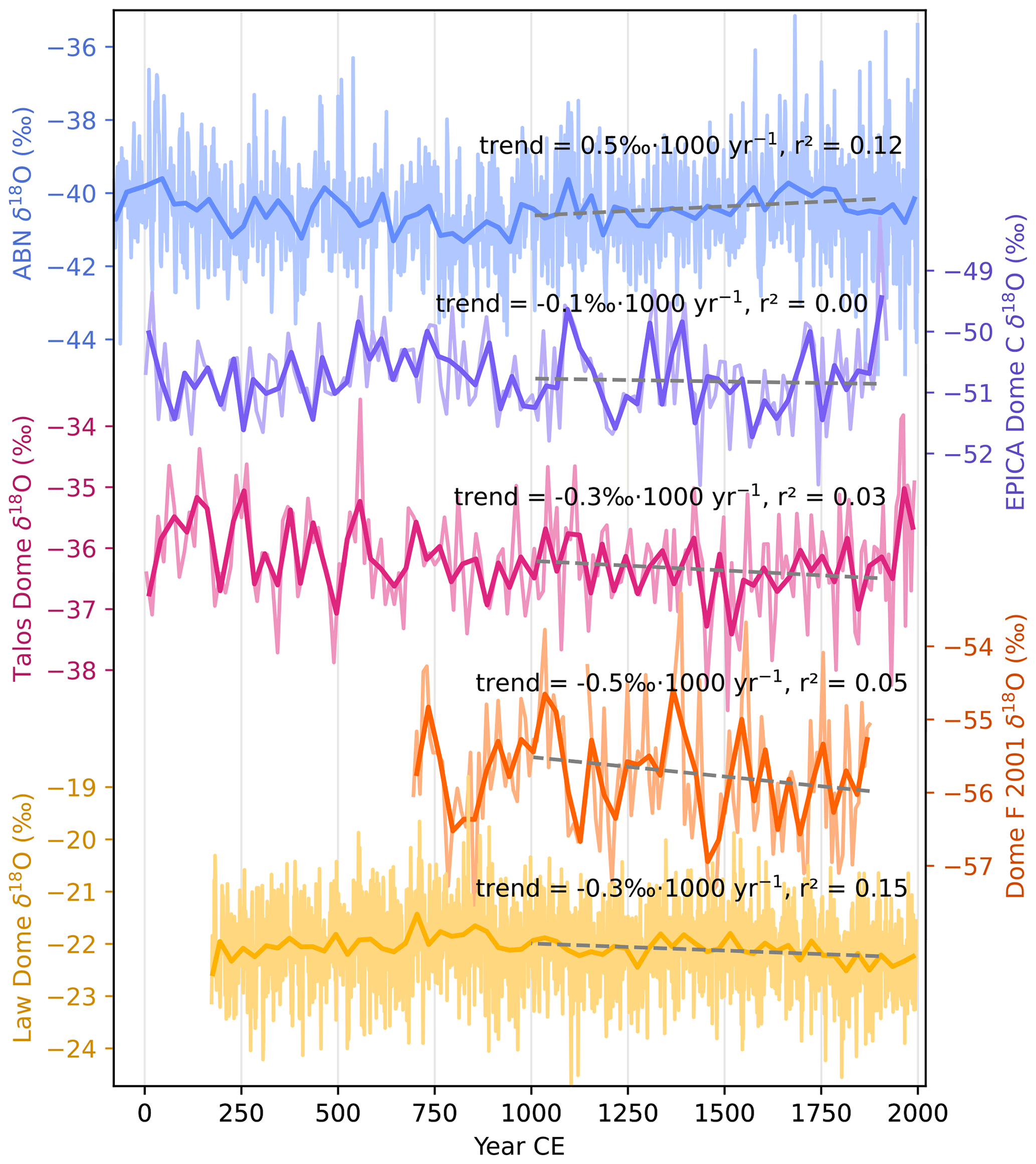
Figure 10Comparison of δ18O records from the ABN1314 core and a selection of nearby ice cores from the Antarctica2k database (Stenni et al., 2017). Thin lines: full resolution, thick lines: resampled at 30-year resolution. Trends are computed from the 30-year resampled series and are significant if r2 > 0.13 (p value < 0.05, n= 31).
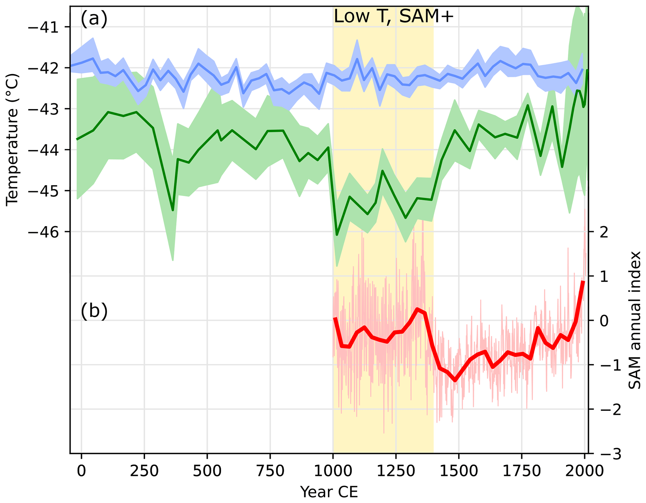
Figure 11(a) δ18O temperature and 15Nexcess temperature reconstructions (this study). Error shading is the same as in Fig. 9. (b) Southern Annual Mode (SAM) annual reconstruction (Dätwyler et al., 2018). The annual resolution of the SAM index is represented by thin lines, and thick lines are the 30-year average for both δ18O temperature and SAM; 15Nexcess temperature has a resolution of about 45 years. Yellow shading highlights the 1000–1400 CE period during which the 15Nexcess temperature is significantly colder, in phase with a positive SAM index.
In particular, in the 15Nexcess and borehole-based reconstruction (Fig. 11a), the temperature at ABN varies between −44.5 and −43 ∘C after 1750 CE but stabilizes at an average of −42.5 ∘C after 1975 CE. After 1900 CE, the temperature inversion is mainly constrained by the borehole temperature, and this warmer phase can be seen in the steepening gradient of the temperature above 100 m below the surface (Fig. 3). This temperature of −42.5 ∘C is about 1 ∘C warmer than the 1500–1850 CE average and could reveal the effect of recent warming in East Antarctica. This surface warming at ABN is unlikely to be caused by a topographic change as the flattening slope near the drilling site (Fig. 9) would on the contrary favour the slowing of katabatic winds and surface cooling by strengthening of the near-surface temperature inversion. The absence of further warming on the East Antarctic plateau after 1975 is consistent with observations and could be related to the compensation effect associated with the positive trend in the Southern Annular Mode in the later part of the 20th century (Nicolas and Bromwich, 2014; Fogt and Marshall, 2020). A similar warming of about 1 ∘C inferred from East Antarctic borehole temperatures has been reported in locations near the ice divide of Dronning Maud Land but was equivocal, as a borehole off the divide showed a possible cooling trend except for the most recent couple of years (Muto et al., 2011). The 15Nexcess and borehole temperature reconstruction provides new insight on the climate of East Antarctica that may complement the δ18O records in this region. Three independent sources of data support this varying temperature history: the borehole temperature, the gas 15Nexcess, and the lock-in depth. Together they consolidate the evidence that annual surface temperature changed with a greater amplitude than what δ18O suggests.
In the southern high latitudes, the Southern Annular Mode (SAM) describes the main mode of geopotential variability (Limpasuvan and Hartmann, 1999), led by meridional pressure differences (Gong and Wang, 1999). This results in zonally symmetric variability with a visible effect on Antarctic surface temperatures (van den Broeke and van Lipzig, 2003). On the East Antarctic plateau, SAM phase and surface temperature are anti-correlated because a stronger meridional pressure gradient is associated with reduced poleward heat transport (Marshall and Thompson, 2016), and the SAM signature is found in the temperature at the ABN site, but SAM does not affect δ18O significantly (Servettaz et al., 2020). On the timescale of a thousand years, the annual SAM has been reconstructed from paleoclimate proxies sensitive to SAM-related temperature anomalies (Dätwyler et al., 2018; Fig. 11b). The 15Nexcess temperature cold interval during 1000–1400 CE co-occurs with a positive phase of the SAM, and then the shift to a strongly negative SAM accompanies the warming at ABN between 1400 and 1500 CE. While this temperature pattern matches the SAM variability, the temperature evolution over the latter half of the last millennium is not explained by SAM changes, as both 15Nexcess temperature and SAM follow an increasing trend. SAM may play a role but is not clearly the only source of surface temperature variability.
We have reconstructed past temperature variability over the last 2000 years from an ice core drilled at Aurora Basin North (ABN), inland East Antarctica. We used two temperature reconstructions: (1) based on water stable isotopes (δ18O) and (2) by inversion of a diffusion model matching borehole temperature and past temperature gradients recorded in gas stable isotopes (15Nexcess). The ABN drilling site is located far from a divide, so we carefully took the ice flow into account when estimating the past temperature, and we were able discuss the climate variability in East Antarctica at a high resolution for the past 2000 years.
The two temperature reconstructions from the same ice core show major differences that are attributed to the difference of spatial and temporal significance of the proxies used: the water stable isotopes acquire their signal during condensation in the atmosphere and are accumulated sporadically during snowfall events, whereas the borehole temperature and gases are constantly exchanging with snow surface conditions and thus integrate the snow surface temperature over a few decades. While the δ18O temperature reconstruction shows little to no trend over the past 2000 years, consistent with other East Antarctic plateau ice cores, the 15Nexcess and borehole temperature inversion suggest that surface temperature varied with an amplitude of about 2 ∘C. A cold period during 1000–1400 CE matches a positive phase of the Southern Annular Mode (SAM), known to have a cooling effect on most of Antarctica (Marshall and Thompson, 2016). The warming trend from the second half of the last millennium while the SAM phase is increasingly positive implies a temperature control through other mechanisms as well. Prevalent cold and dry winters during cold periods may explain both the inability of water isotopes to record temperature changes and the lower-than-average surface snow temperature. The 15Nexcess temperature reconstruction seems to better track surface temperature changes than δ18O, although with a lower temporal resolution. This work highlights the importance of using diverse proxies in temperature reconstructions and motivates further studies to understand the proxies used, beyond simple linear relationships.
A1 Calibration and corrections of isotopic composition of gases
Measurements of gases from ice cores and their correction have been extensively described by Severinghaus et al. (2001). In addition to their corrections of pressure imbalance (Appendix A1.1) and chemical slope (Appendix A1.2), we introduce a specific correction for focus drift (Appendix A1.3) before the normalization to the atmosphere, which is the standard for the gas isotopes measured in this study (Appendix A1.4).
A1.1 Pressure imbalance correction
In a dual-inlet mass spectrometer, two bellows alternatively supply gas to the spectrometer source. Possible differences in the pressure of each bellow can influence the beam intensity and thus measured δ values. This effect is quantified using daily-determined pressure imbalance slopes (PISs), where the volume in the bellows is forced into an asymmetrical state to evaluate the effect on isotope ratios (for example Fig. A1). The pressure imbalance (ΔP) is defined by the difference of intensity (int) between the sample and standard of the main gas measured (28N2 in nitrogen configuration or 40Ar in argon configuration).
Isotopic measurements are then corrected using daily PIS and imbalance during measurement, as shown in Eq. (A2).
Equivalent slopes and corrections were performed for δ15N. ΔP is calculated with intensities averaged on entire blocks for standards (11 integrations) and samples (10 integrations). Pressure imbalance correction is applied block by block, and the standard deviation of five blocks of argon in a sequence typically decreases from 0.020 ‰ to 0.015 ‰ (0.005 ‰ improvement). The pressure-imbalance-corrected values are compared to raw values in Fig. A2. The pooled standard deviation (PSD) in Fig. A2 is given for ice replicates and is therefore larger than the standard deviation of block-averaged δ values within a sequence for a unique sample.
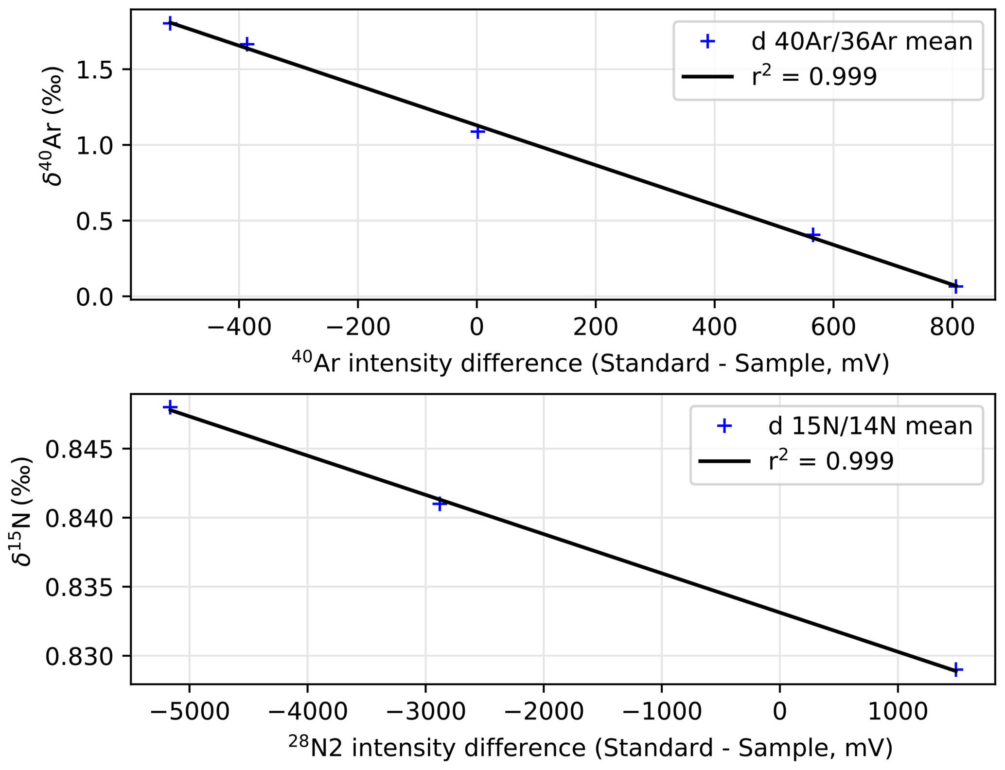
Figure A1Variability of δ40Ar and δ15N as a function of intensity difference between the sample and standard.
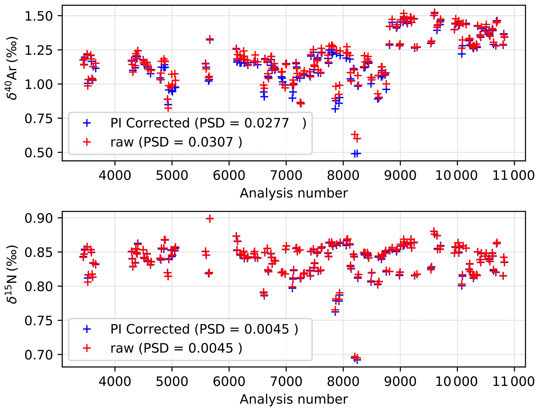
Figure A2Comparison of δ40Ar and δ15N before and after pressure imbalance correction for all the measurements. The analysis number corresponds to the number of blocks, and measurements were performed between February and December of 2019. Pooled standard deviation (PSD) values of each series are indicated in the captions.
A1.2 Chemical slope correction
The gas supplied to the spectrometer and ionized by the filament is a mixture of argon (about 1 %) in nitrogen (about 99 %) with very few other gases. The elemental ratio of argon to nitrogen can modify how effectively the argon will be ionized because of charge transfer in the source. Therefore, the relative quantity of argon in the mixture can affect the δ40Ar measured by the spectrometer. The chemical ratio effect is quantified by preparing collector tubes of pure nitrogen with a varying amount of standard argon of known isotopic composition. We determine the ratio of Ar N2 with peak jumping and measure the δ40Ar over five blocks for each mixture. The slope is defined in Eq. (A4) and illustrated by Fig. A3.
We apply the chemical slope correction to the δ40Ar values averaged over a full sequence because the elemental mixture does not change within a sample.
The chemical slope was measured after each change in the filament and if the filament was put in contact with air, as it may cause a change in the ionization rate and therefore the chemical slope. Consequently, we only have three chemical slope measurements for 8 months: at the beginning, in the middle, and at the end. This correction does not result in an immediate improvement of the pooled standard deviation (Fig. A4) because the chemical slope error is partly compensated for by a drift error (next section), so correcting only the first effect induces a small increase in the sample difference.
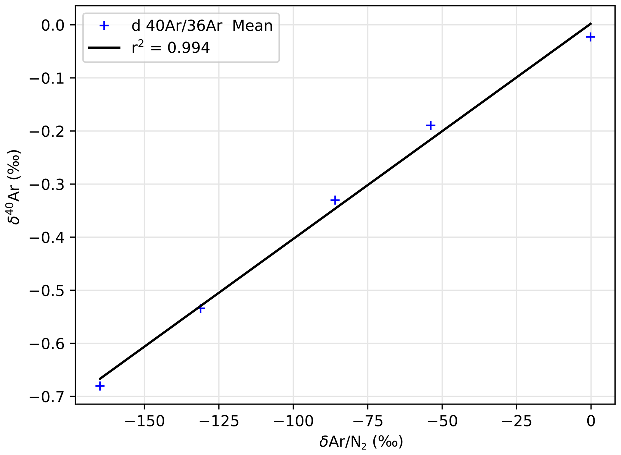
Figure A3Chemical slope: variability of δ40Ar versus δAr N2. A larger concentration of Ar in the gas mixture introduced into the spectrometer tends to increase the δ40Ar values measured.
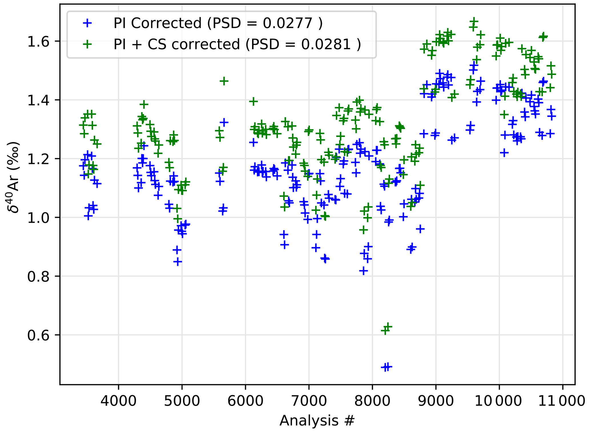
Figure A4Correction of the chemical slope effect on δ40Ar. Because the gas trapped in ice is generally argon-depleted compared to the atmosphere, the chemical-slope-corrected values (green) are greater than non-corrected values (blue). Pooled standard deviation (PSD) values of each series are indicated in the captions.
A1.3 Drift correction
In addition to the previously published correction, we determined that drifts around analysis 5000 or 7200 were caused by the spectrometer focus changing over time, causing a strong variability of δ40Ar and PIS. This drift could not be easily resolved because it only appeared after weeks of measurements. This issue was temporarily fixed with regular autofocus, but we needed a thorough recalibration of the focus parameters to make it more stable. Later, we fully recalibrated the spectrometer focus, causing a large change in raw δ values for both samples and standards used for calibration (from the analysis number 8800). Fortunately, the focus changes proportionally shifted the values of PIS and the δ40Ar and did not affect δ15N values, which we attribute to nitrogen being the most abundant gas supplied to the spectrometer. To distinguish from potential pressure-gradient-induced fractionation during sample preparation, which would affect both δ40Ar and δ15N proportionally to their mass, we removed the gravitational fractionation of δ40Ar using the δ15N. By doing so, the drift effect on δ40Ar could be quantified against the PIS40Ar as shown in Fig. A5. We define a drift slope as the non-gravitational fractionation of Ar versus the PIS40Ar in Eq. (A5).
Using the drift slope, we then correct δ40Ar values.
This improved the precision as attested by PSD of δ40Ar in replicates that dropped from 0.028 ‰ to 0.013 ‰ (Fig. A6). Note that if we apply the drift correction without the chemical slope correction, the PSD only improves to 0.016 ‰ (not shown), showing the importance of chemical slope correction prior to the drift correction.
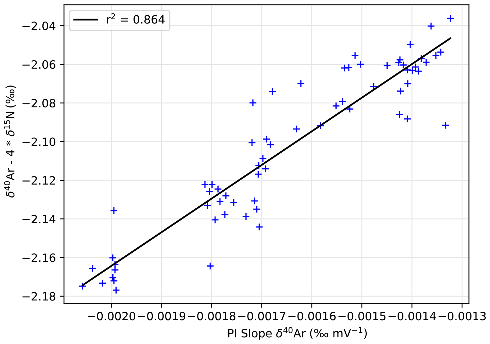
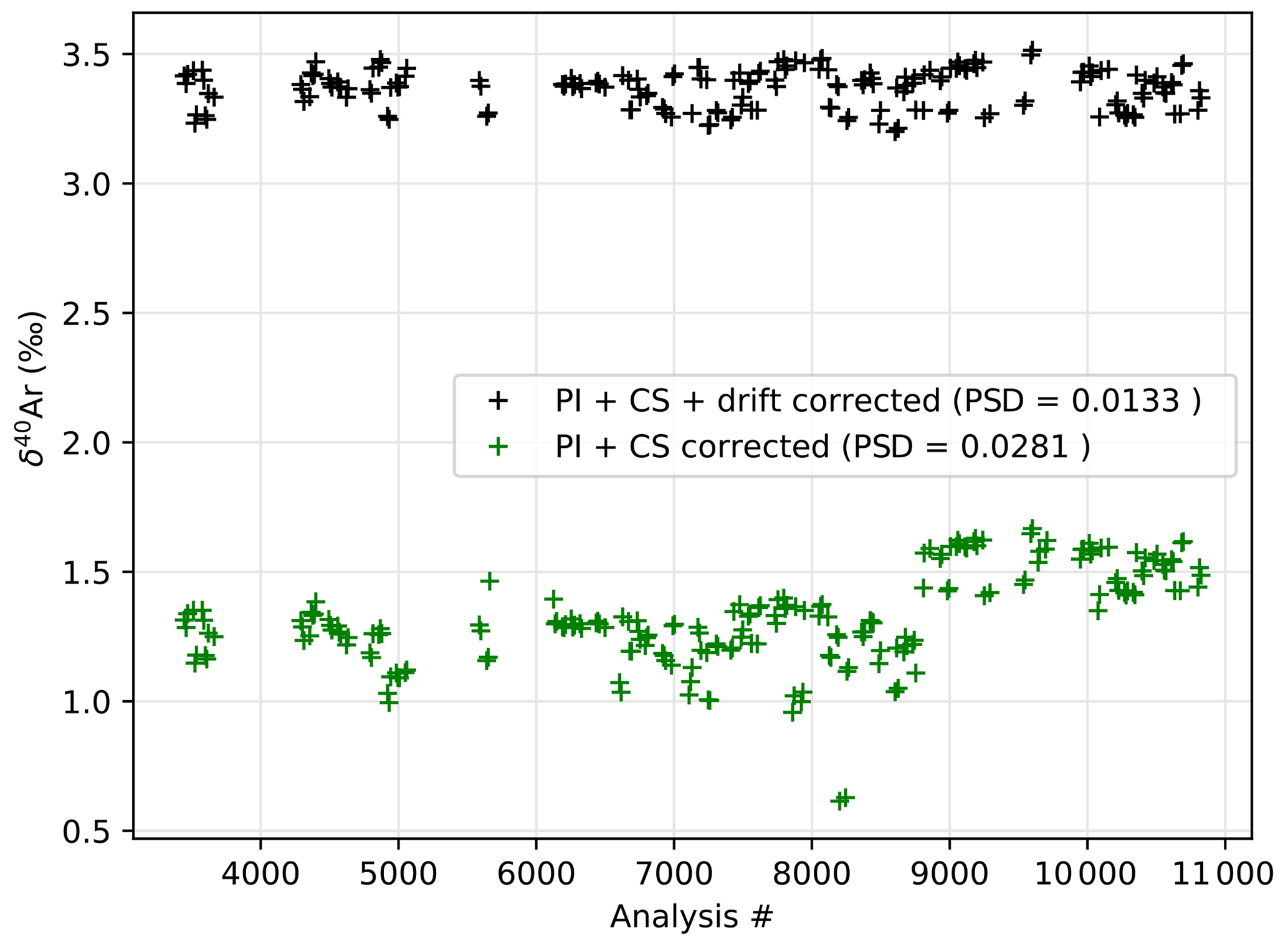
Figure A6Correction of the drift effect on δ40Ar. Pooled standard deviation (PSD) values of each series are indicated in the captions.
A1.4 Normalization to the atmosphere
All δ values are defined as the relative difference to a standard. For argon and nitrogen gases, the standard is the atmospheric air (IAEA, 1995). Two to three air standards were prepared weekly from a bottle of air captured in Saclay in 2019. The same sample preparation and corrections are applied to the air standard, as would be made for gas extracted from an ice sample. In total, 83 replicates of air standards were measured, with a standard deviation after all corrections of 0.0052 ‰ for δ15N, 0.0188 ‰ for δ40Ar, and 0.0029 ‰ for 15Nexcess. We believe that some of the error in the δ15N and δ40Ar is due to the sampling processing in the gas line, with gas being released into empty tubing, causing large pressure differences that are known to fractionate the isotopes. Even though we try to allow some time to equilibrate, a small fractionation probably remains. This affects the two sample replicates differently because they are processed separately, but both nitrogen and argon in the same sample are affected by the same pressure changes and resulting fractionation. Given that 15Nexcess is defined as the mass-weighted difference between the two isotopic ratios, some of the fractionation induced by sample processing may cancel out, and therefore the pooled standard deviation in 15Nexcess between the two samples is smaller than δ15N or δ40Ar alone (0.0137 ‰ for δ40Ar and 0.0036 ‰ for δ15N).
We use weekly averages of two to three measurements of δ15N and δ40Ar in atmospheric air to normalize the ice measurements of the corresponding week (Fig. A7). By doing this correction weekly, we further correct any drift that can happen, as it would affect both our gas trapped in ice and atmospheric air standards in the same manner.
Normalization of the δ40Ar and δ15N of ice samples does not change the pooled standard deviation because the two replicates are corrected by the same amount. However, it corrects the absolute value needed for quantification of gravitational and thermal effects.
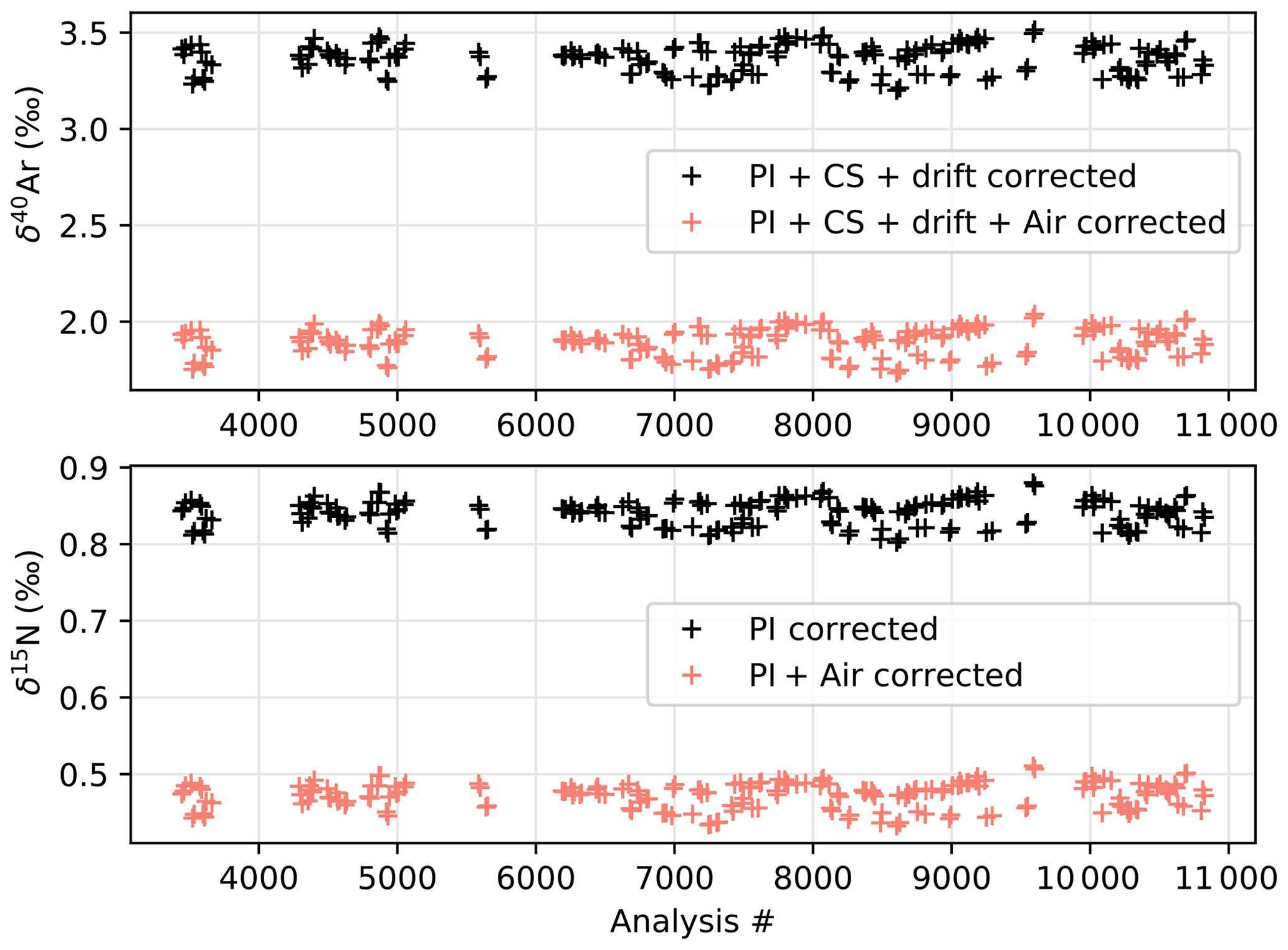
Figure A7Normalization to the atmosphere. The values are subsequently given in per mill (‰) versus atmosphere. The pooled standard deviation is unchanged with normalization because the same correction is applied for both duplicates.
A2 Age Models
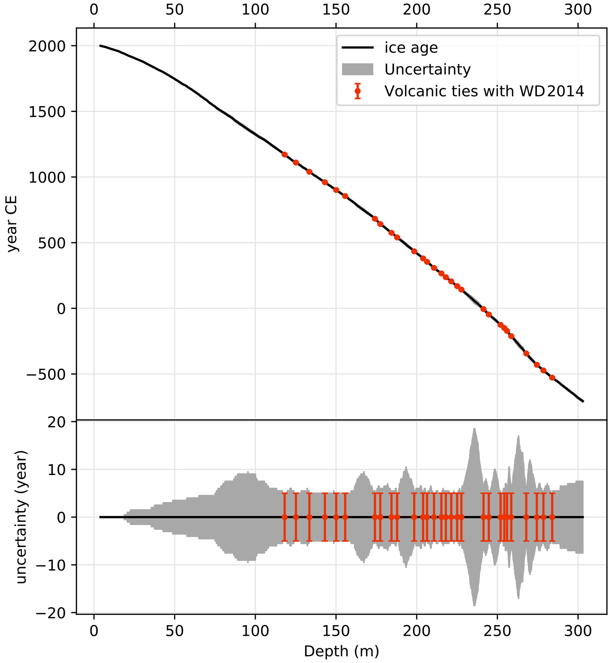
Figure A8Age model for the ABN1314 core. The grey shading indicates cumulated uncertainties in annual layer counting. Volcanic horizons were identified on the sulfur record, tied to the ages of volcanic events on the WD2014 timescale (Sigl et al., 2015, 2016), and given a ±5-year uncertainty, corresponding to the maximum intrinsic uncertainties in the WD2014 timescale for this period.
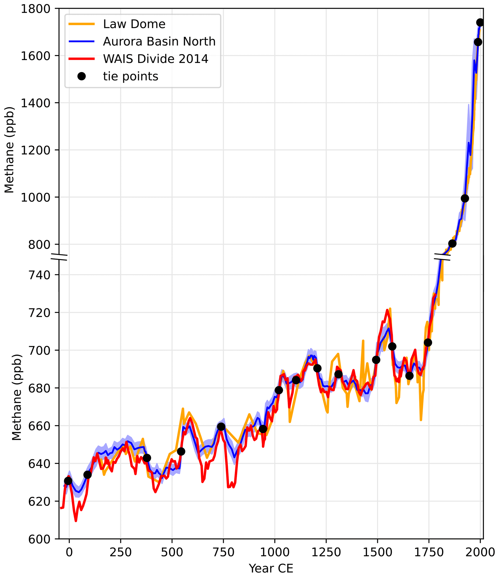
Figure A9Methane concentration in trapped air in ABN1314 (blue) averaged on 1 m sections (the light blue shading shows the 1σ standard deviation of measurements in the 1 m section, measured on a continuous flow analysis system) for the West Antarctic Ice Sheet (WAIS) Divide (red, Mitchell et al., 2011) and Law Dome (orange, Rubino et al., 2019) on the WD2014 gas timescale (Sigl et al., 2015, 2016). The vertical axis changes scale with an axis break at 750 ppb.
A3 Ice-flow-related changes
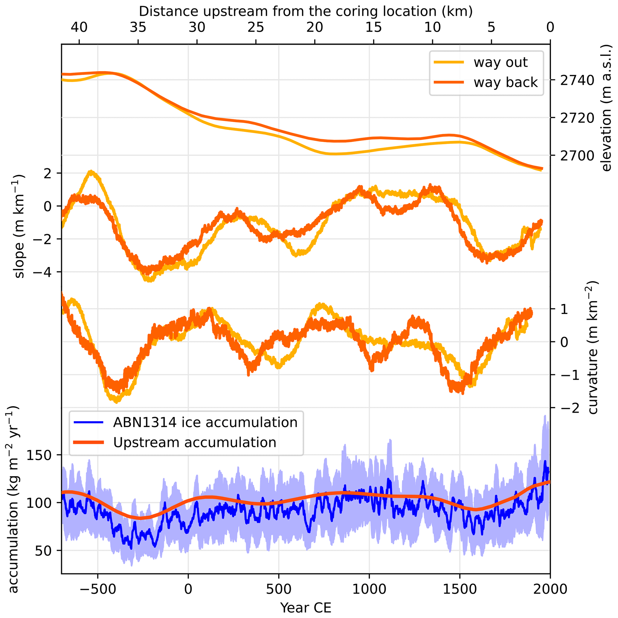
Figure A10Upstream elevation, slope, curvature, and accumulation compared to the ice accumulation in the ABN1314 core. ABN ice accumulation was calculated with the layer thickness from annual layer counting as well as the density profile measured by weighing known volumes of the ice core and is shown with a 20-year running mean to smooth out the reconstruction. The light blue shading shows the 20-year standard deviation. Upstream accumulation is estimated by integrating the ice mass between the surface and first isochron reflector in the ground-penetrating radar profile. We used the density profile measured in the ABN1314 ice core to estimate the mass, assuming the density upstream follows a similar profile, and we inferred the age of the isochron from the age at the corresponding layer in the ABN1314 core. Ice movement since deposition is estimated by varying the spatial length of the upstream accumulation record sampled to maximize the correlation with the 2700-year temporal accumulation record from the ABN ice core (lower panel). Elevation was determined with truck GPS position during upstream radar profiling. The profile was taken twice: moving away from the coring site (way out) and going back to the coring site (way back). Original GPS coordinates were not taken in optimal conditions (moving truck), hence the uncertainty.
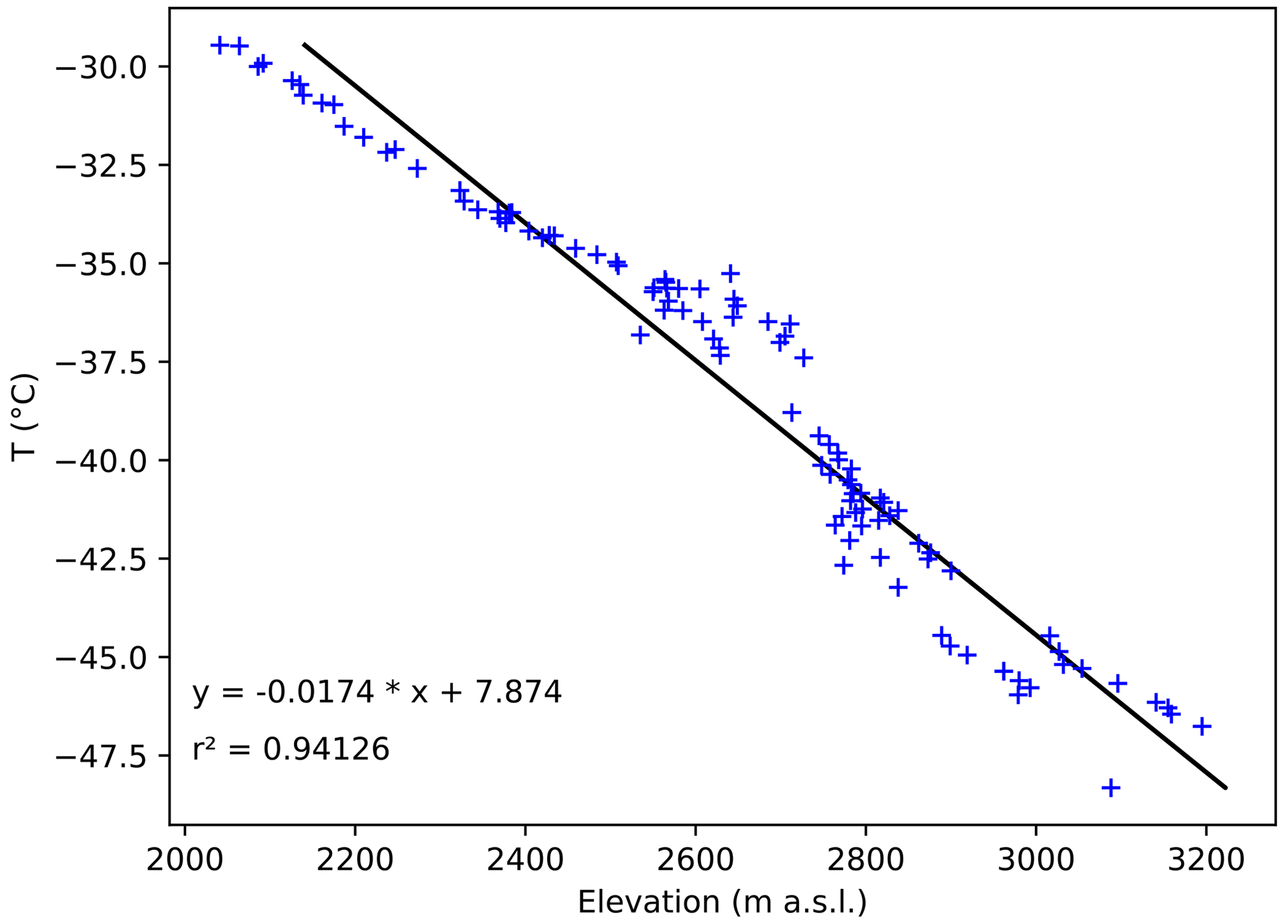
Figure A11Temperature–elevation slope in the 2000–3250 m.a.s.l. elevation range in East Antarctic traverses with site temperature estimations (Xiao et al., 2013; Pang et al., 2015).
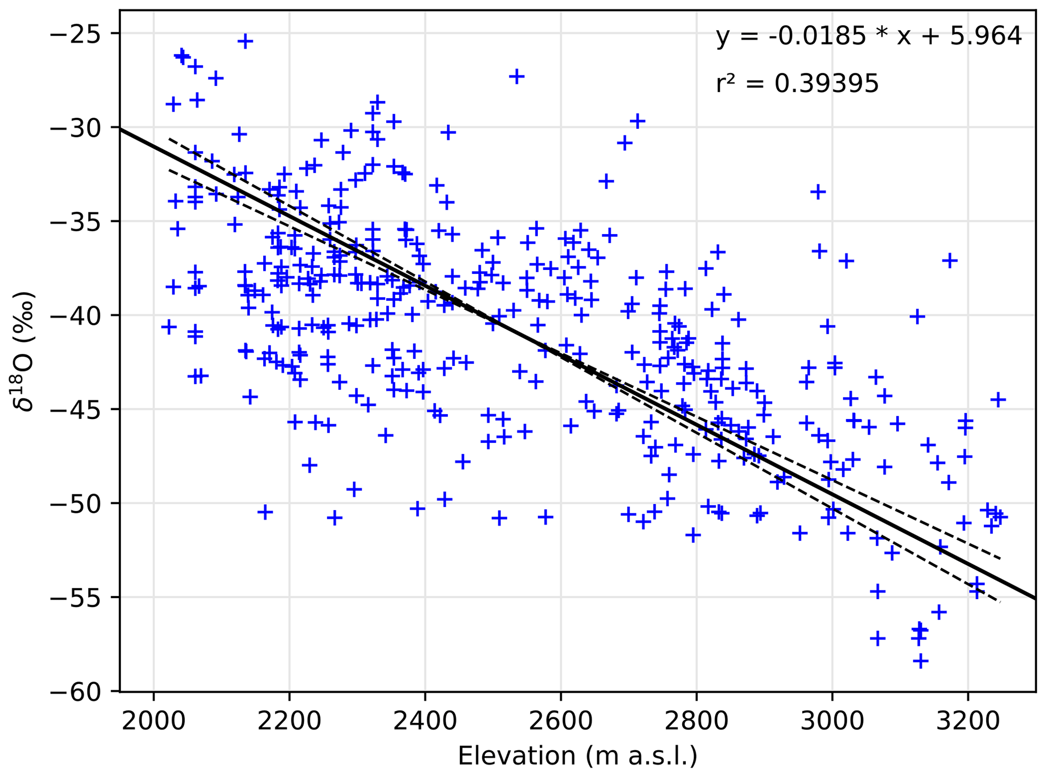
Figure A12δ18O–elevation slopes in surface snow studies: Zongshan to Dome A traverses (Xiao et al., 2013; Pang et al., 2015) and extended Antarctic snow database (Goursaud et al., 2018). We restricted our slope to sites at elevations between 2000 and 3250 m a.s.l. and longitudes from 80 to 160∘ E.
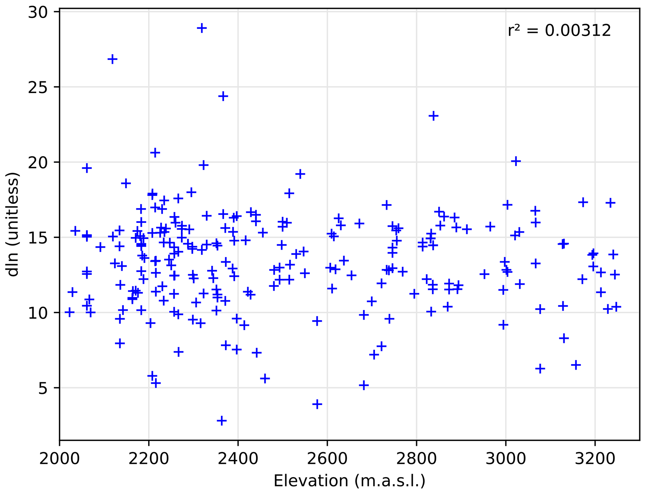
Figure A13The dln–elevation scatter plot in the Goursaud et al. (2018) database, restricted to sites at elevations between 2000 and 3250 m.a.s.l. and longitudes from 80 to 160∘ E.
A4 Advection–diffusion ice model tuning
A4.1 Parameters
The model simulates the diffusion and advection of temperature in the ice. Given an initial state, the temperature will diffuse depending on boundary conditions such as surface temperature, advection due to accumulation of ice, compaction, and bottom temperature. We set the compaction to follow the ice density profile measured in the core, under the assumption that it did not change significantly in the past. Surface temperature is inferred from different temperature scenarios, plus a sinusoidal seasonal cycle for which an amplitude of 13.7 ∘C has been deduced from the temperature cycle at the ABN automatic weather station. Bottom temperature is constrained by a constant geothermal heat flux of 65 mW m−2 for the Aurora Basin (Maule, 2005; Martos et al., 2017). Temperature diffusion simulations start at 2000 BCE and last for 4014 years, allowing for flexibility in the first ∼ 2000 years for which we have no gas constraints. For the past 2700 years (700 BCE onwards), we use the accumulation obtained with annual layer counting with a 20-year running average (as shown in Fig. A10). Previous this date, we use the average accumulation of 94 kg m2 yr−1 (Akers et al., 2022). The model is also highly dependent on the initial temperature profile in the ice.
The ice thickness is suspected to have varied over time both spatially and temporally. Upstream of the ABN coring location, the ice about is 500 m thicker than the current 3500 m, mainly because bedrock is deeper in the central part of the Aurora Basin. We assume that temporal variations of ice thickness in the Aurora Basin during the past 4000 years are much smaller than this. For simplification, we use an averaged thickness of 3700 m over the past 4000 years. Changes in ice thickness of 500 m caused by a surface change in accumulation may affect the temperature gradient in the upper ice column (Morgan et al., 2022), but thickness changes associated with glacial flow should not have a significant impact at the scale of 2000 years because most of the ice deformation occurs at depth (Wang and Warner, 1999; Doyle et al., 2018), and equilibration time between the bedrock and the surface is of the order of magnitude of 10 000 years. The accumulation history used in the model is inferred from the ice core accumulation with a 20-year smoothing.
Finally, the diffusion model outputs gradients of temperature between the surface and a lock-in depth, which is inferred from the lock-in depth history determined in Sect. 3.2 of the main text. Uncertainties of ±4 m in the lock-in depth result in ±0.03 ∘C in the surface to lock-in depth temperature gradient, 10 times smaller than the uncertainties in the ΔT estimated from the gases.
A4.2 Initialization with consideration of ice flow
We account for the long-term influence of ABN site displacement on the temperature scenarios using a transient state initialization. Most deformations associated with ice flow occur in the bottom layers of ice in contact with the rocks, where the temperature is near the melting point (Wang and Warner, 1999; Doyle et al., 2018). The uppermost column of ice is advected rather uniformly, so we can simply consider surface temperature changes from a Lagrangian point of view, whereby we follow the column of ice under ABN as it flows. Therefore, we consider two components of temperature changes: spatial temperature changes due to the displacement of ice and climatic temperature changes. For simplification, and because our simulation only spans the last 4000 years, we consider the surface topography to be constant and assume that climatic temperature changes spatially vary homogeneously in the range of 40 km. This allows us to simply run the diffusion–advection model with a single dimension (depth).
We chose to initialize the model with a transient state profile rather than a stationary temperature profile to simulate the presence of cold ice advected under the ABN coring site and better match the −2.5 ∘C temperature gradient observed in the borehole measurement. The initialization is performed with a transient state temperature simulation, in which we equilibrated the ice column with a surface temperature of −61 ∘C for 20 000 years, then simulate the deglaciation and the Holocene with the temperature history from Dome C (Jouzel et al., 2007), added to ice-flow-related temperature changes from modern surface temperature (Agosta et al., 2019) and ice flow velocities (Mouginot et al., 2019). The temperature history used during initialization is shown in Fig. A14. The initialization run is unique and starts from 30 000 to 2000 BCE. The past accumulation during initialization is set at 40 % of the average ABN accumulation, increasing to 80 % during deglaciation and ramping up to 100 % at 2000 BCE. The ratio of accumulation between the Last Glacial Maximum and the late Holocene is set to be roughly the same as Dome C (Wolff et al., 2010) and WAIS Divide (Buizert et al., 2015). Arguably, the ice flow was slower than the modern day in the glacial period, which would result in smaller temperature changes if modelled correctly, but such precision is not needed in the initialization of the model. This transient initialization produces a temperature profile with a strong gradient, which can match the observations within 0.5 ∘C if the simulation is continued until 2014 CE (Fig. A15), and is thus a good starting point for the temperature simulations.
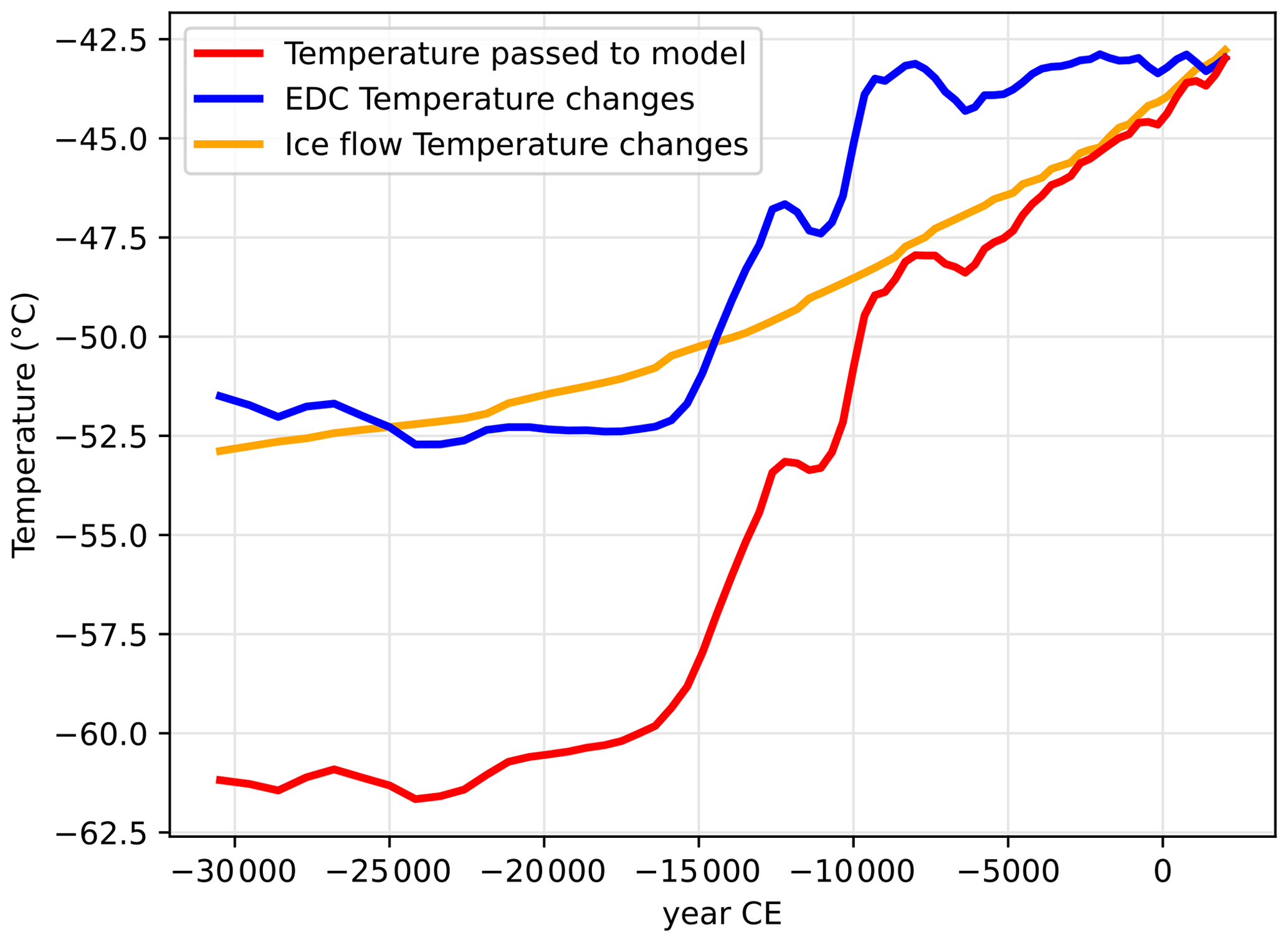
Figure A14Base surface temperature passed to the model in the transient state initialization, which runs from 30 000 to 2000 BCE, and the unperturbed simulation from 2000 BCE to 2014 CE. The red line shows the total temperature changes, the blue line shows EDC temperature changes (Jouzel et al., 2007; shifted to match ABN modern temperature), and the orange line shows the ice-flow-related temperature changes from a simple interpolation of modern-day Antarctic surface temperature along the estimated back-projected position of ABN using modern flow speeds (Mouginot et al., 2019).
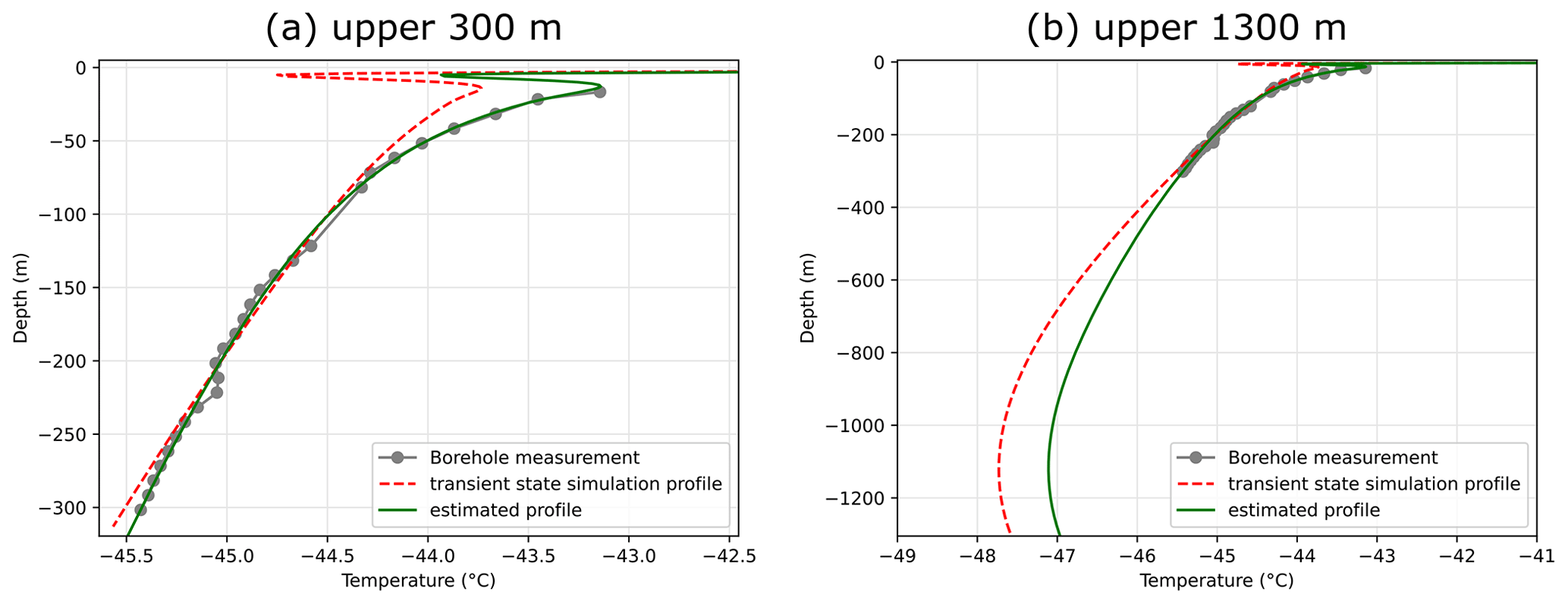
Figure A15Temperature profile obtained after the transient state initialization (red dashed line) compared to the borehole temperature profile (grey points) and the estimated temperature profile after inversion (green) on the upper 300 m (a) and the upper 1300 m (b) of the ice column.
A4.3 Temperature perturbation simulations
Starting from the transient state profile of temperature at 2000 BCE, we start simulations following the same base surface temperature forcing (later part of Fig. A14) and add a “triangle-shaped” perturbation in each simulation, with an additional temperature increase ramping up to +1 ∘C. The added perturbation increases over the course of 10 years then decreases in another 10 years to return to the base surface temperature forcing for the remainder of the simulation. The next simulation uses a perturbation that is shifted in time by 10 years. A few longer-lasting perturbations are used in the 2000 BCE–0 CE period, for which the constraints are low because of the absence of gas data, and the climate information is not used in the results of this study. We perform a total of 220 simulations with perturbations at different times in the run.
A5 Parameters of the temperature inversion
A5.1 Shift of the 15Nexcess mean value
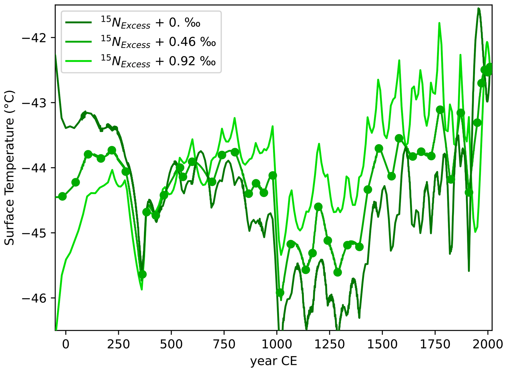
Figure A16History of temperature obtained with inversion of borehole and temperature gradients obtained with 15Nexcess using different correction values for 15Nexcess. Not correcting or too strongly correcting the 15Nexcess causes the temperature reconstruction to squeeze high-frequency sawtooth-shaped variations between ages for which we have gas data points, represented by the dots.
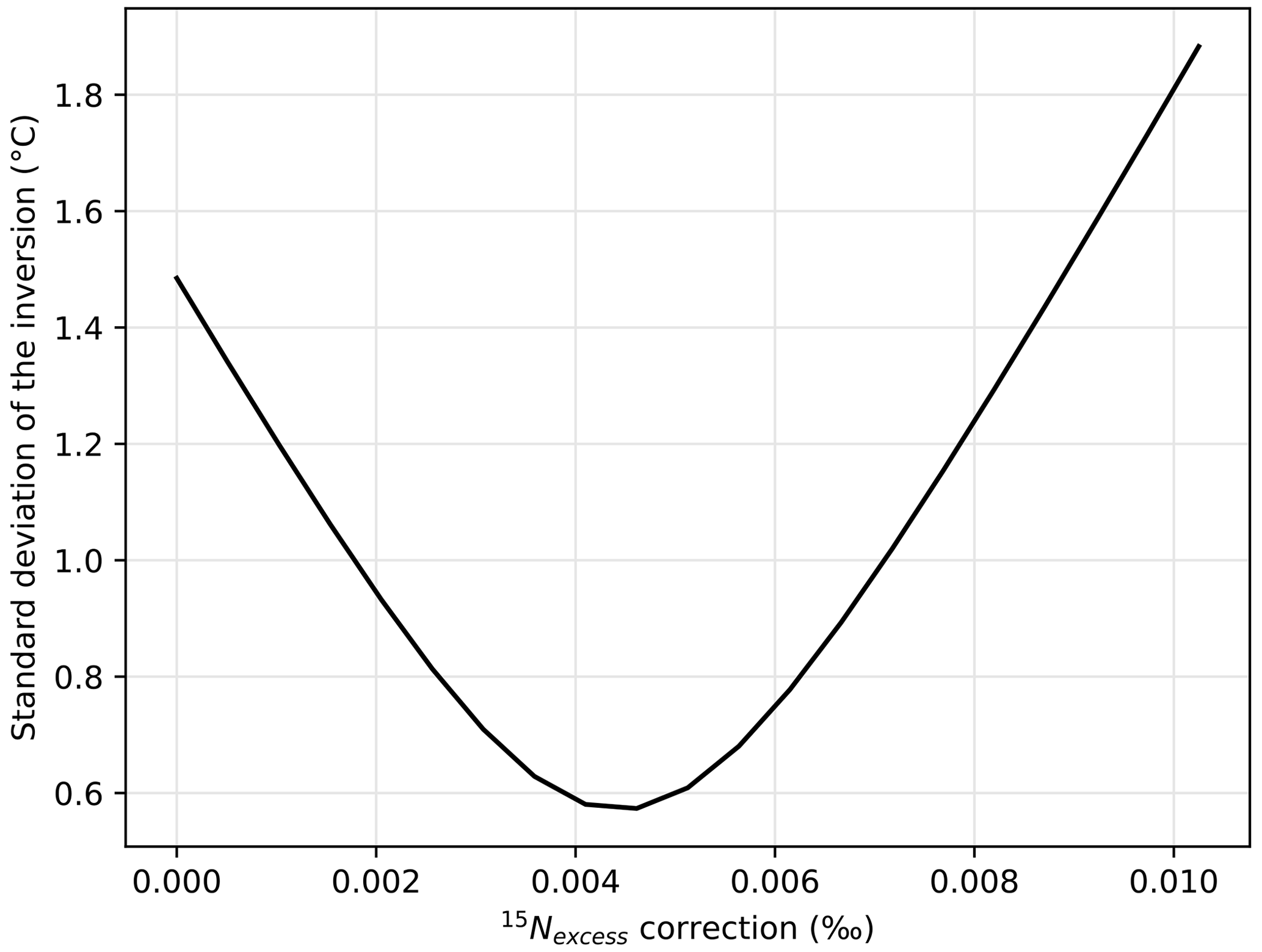
Figure A17Standard deviation of the history of temperature depending on the value used for 15Nexcess correction. A value of 0.0046 ‰ is best to minimize the intrinsic variability of the reconstruction and match both datasets.
A5.2 Uncertainty parameters
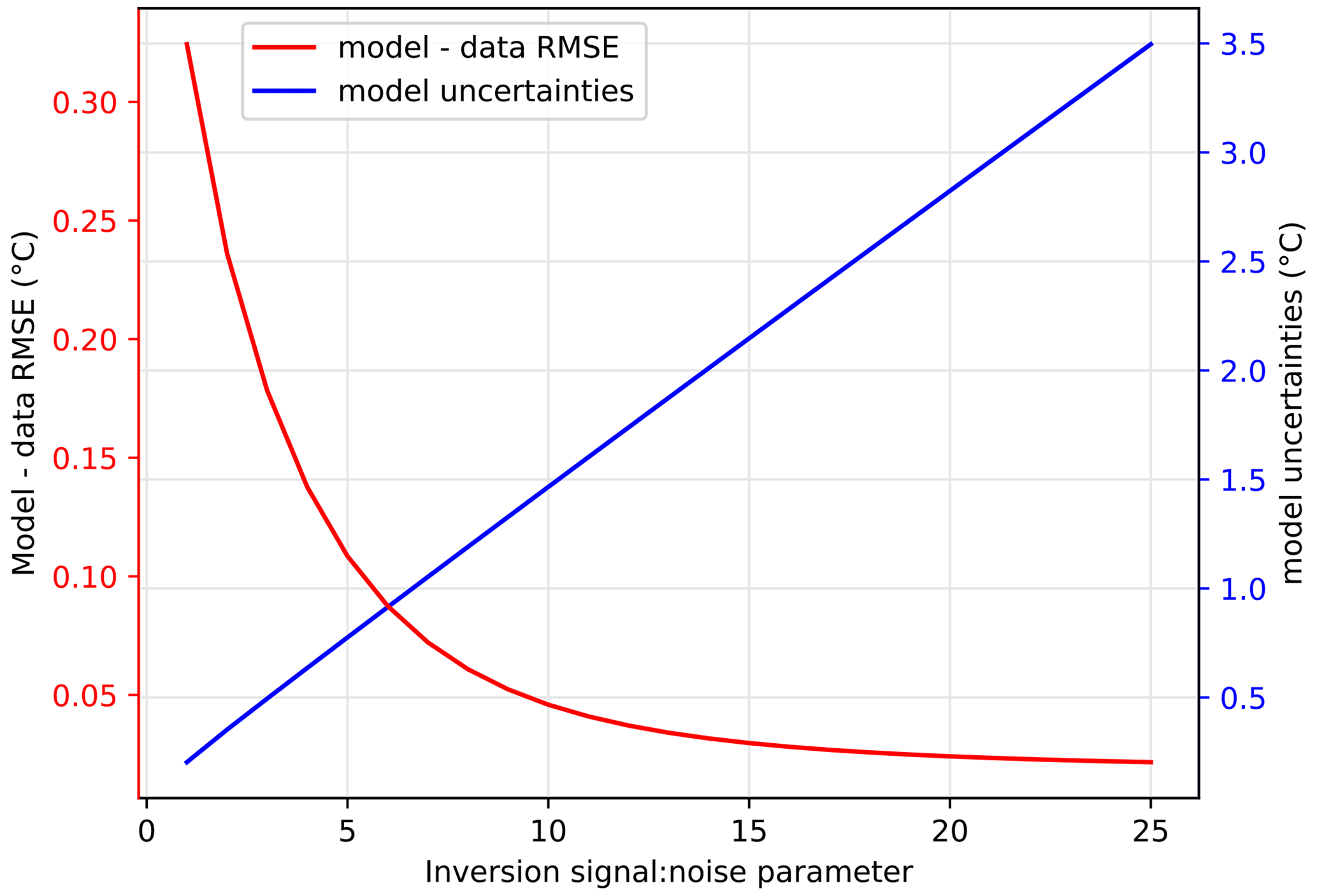
Figure A18Root mean square error (RMSE, red) between temperature reconstruction and temperature data passed to the inversion and reconstruction uncertainty (blue) as a function of the signal-to-noise parameter. A signal-to-noise ratio that is too low results in an inversion that is too smooth with high model–data mismatch, whereas a parameter that is too high increases the resulting inversion uncertainty to allow for more flexibility.
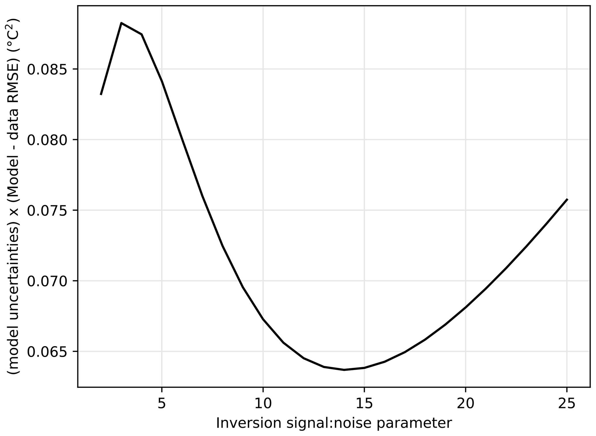
Figure A19Cost function of the reconstruction as a function of the signal-to-noise parameter used in the inversion. A value of 14 is best to ensure that the inversion matches the constraints and minimize its uncertainty.
A5.3 Age significance of data points in the reconstruction
The diffusion of temperature in the firn depends on both snow and ice properties but also the accumulation rate at the ice core site. At the West Antarctic Ice Sheet Divide (WAIS Divide), the temperature measured at depths corresponding to the last millennium was estimated to integrate temperature with a smoothing window of several hundred years (Orsi et al., 2012); for ABN where the ice accumulation is half as high as WAIS Divide, we expect even greater smoothing windows. The temporal range of temperature changes recorded by 15Nexcess at ABN is limited at the minimum by the diffusion time of gases between the surface and the lock-in zone and at maximum by the smoothing out of the temperature gradient by the temperature diffusion in the ice column. At the North Greenland Eemian Ice Drilling (NEEM) site, gases take on average 10 years to diffuse down to the lock-in depth of 63 m (Witrant et al., 2012); we expect that at ABN, where the lock-in depth is about 30 m deeper, the gases will take slightly longer to equilibrate in the diffusive column, so a temperature gradient maintained for approximately 20 years should be effectively recorded in the 15Nexcess.
In addition, we further reduced the time resolution of gas-based reconstruction by averaging the isotopic values in 5 m windows, with an expected age range of about 45 years. Lastly, we applied a smoothing in the inversion to limit the variability of neighbouring points by forcing a covariance in the reconstruction. The covariance parameter was set to be exponentially decreasing with age difference, with a 0.5 covariance reached at 70 years of difference. Therefore, the reconstruction includes multiple gas data points for each inversion point, strengthening the confidence in the reconstructed temperature. In our figures, we chose to represent the inversion at the time resolution of points when there is a gas-based temperature constraint.
Data created during this study, including age models for ABN1314 ice and gases, water isotopes (δ18O and δD), gas isotopes (δ15N and δ40Ar), borehole temperature, methane, and ice density, as well as temperature reconstructions, are accessible in a repository on the Australian Antarctic Division data centre web site (Moy et al., 2023, https://doi.org/10.26179/5qyn-xf50).
MC directed the ABN ice core drilling project. AO and AS designed the study. Raw water isotope data were measured and curated by AM. AO designed the gas isotope analysis, and AS performed the gas isotope analysis. TP measured the borehole temperature. AO secured financial resources for gas laboratory analyses and, together with AL, supervised stable isotope interpretations. JMC measured water stable isotopes in the shallow core used for calibration. JMC, XF, and JC measured the methane used for the gas age model. ELM provided upstream GPS elevation profiles and radar reflector surfaces. MC performed the annual layer counting and provided volcanic tie ages for the ice age model. AO adapted the ice diffusion model and designed the inversion algorithm. AS performed the diffusion model simulations. AS and AO interpreted the climate implications of the results. AS wrote the original draft and created the figures. AO, MC, AM, AL, JMC, ELM, TP, XF, and JC contributed to the redaction with comments, suggestions, and corrections on the paper.
At least one of the (co-)authors is a member of the editorial board of Climate of the Past. The peer-review process was guided by an independent editor, and the authors also have no other competing interests to declare.
Publisher’s note: Copernicus Publications remains neutral with regard to jurisdictional claims in published maps and institutional affiliations.
The authors would like to thank the Aurora Basin North field team, in particular Simeon Sheldon for the help with the borehole temperature measurement and Christopher Plummer for help with annual layer counting. We are grateful to the two referees for their comments on the paper.
This research has been supported by the Australian Antarctic Division (grant no. AAS project 4075), the Institut Polaire Français Paul Emile Victor (CHICTABA project no. 1115), and the Institut national des sciences de l'Univers (LEFE project ABN2k).
This paper was edited by Elizabeth Thomas and reviewed by two anonymous referees.
Abram, N. J., McGregor, H. V., Tierney, J. E., Evans, M. N., McKay, N. P., and Kaufman, D. S.: Early onset of industrial-era warming across the oceans and continents, Nature, 536, 411–418, https://doi.org/10.1038/nature19082, 2016.
Agosta, C., Amory, C., Kittel, C., Orsi, A., Favier, V., Gallée, H., van den Broeke, M. R., Lenaerts, J. T. M., van Wessem, J. M., van de Berg, W. J., and Fettweis, X.: Estimation of the Antarctic surface mass balance using the regional climate model MAR (1979–2015) and identification of dominant processes, The Cryosphere, 13, 281–296, https://doi.org/10.5194/tc-13-281-2019, 2019.
Akers, P. D., Savarino, J., Caillon, N., Servettaz, A. P. M., Le Meur, E., Magand, O., Martins, J., Agosta, C., Crockford, P., Kobayashi, K., Hattori, S., Curran, M., van Ommen, T., Jong, L., and Roberts, J. L.: Sunlight-driven nitrate loss records Antarctic surface mass balance, Nat. Commun., 13, 1–10, https://doi.org/10.1038/s41467-022-31855-7, 2022.
Bereiter, B., Kawamura, K., and Severinghaus, J. P.: New methods for measuring atmospheric heavy noble gas isotope and elemental ratios in ice core samples, Rapid Commun. Mass. Sp., 32, 801–814, https://doi.org/10.1002/rcm.8099, 2018.
Buizert, C. and Severinghaus, J. P.: Dispersion in deep polar firn driven by synoptic-scale surface pressure variability, The Cryosphere, 10, 2099–2111, https://doi.org/10.5194/tc-10-2099-2016, 2016.
Buizert, C., Martinerie, P., Petrenko, V. V., Severinghaus, J. P., Trudinger, C. M., Witrant, E., Rosen, J. L., Orsi, A. J., Rubino, M., Etheridge, D. M., Steele, L. P., Hogan, C., Laube, J. C., Sturges, W. T., Levchenko, V. A., Smith, A. M., Levin, I., Conway, T. J., Dlugokencky, E. J., Lang, P. M., Kawamura, K., Jenk, T. M., White, J. W. C., Sowers, T., Schwander, J., and Blunier, T.: Gas transport in firn: multiple-tracer characterisation and model intercomparison for NEEM, Northern Greenland, Atmos. Chem. Phys., 12, 4259–4277, https://doi.org/10.5194/acp-12-4259-2012, 2012.
Buizert, C., Cuffey, K. M., Severinghaus, J. P., Baggenstos, D., Fudge, T. J., Steig, E. J., Markle, B. R., Winstrup, M., Rhodes, R. H., Brook, E. J., Sowers, T. A., Clow, G. D., Cheng, H., Edwards, R. L., Sigl, M., McConnell, J. R., and Taylor, K. C.: The WAIS Divide deep ice core WD2014 chronology – Part 1: Methane synchronization (68–31 ka BP) and the gas age–ice age difference, Clim. Past, 11, 153–173, https://doi.org/10.5194/cp-11-153-2015, 2015.
Casado, M., Orsi, A. J., and Landais, A.: On the limits of climate reconstruction from water stable isotopes in polar ice cores, PAGES Mag., 25, 146–147, https://doi.org/10.22498/pages.25.3.146, 2017.
Casado, M., Landais, A., Picard, G., Münch, T., Laepple, T., Stenni, B., Dreossi, G., Ekaykin, A., Arnaud, L., Genthon, C., Touzeau, A., Masson-Delmotte, V., and Jouzel, J.: Archival processes of the water stable isotope signal in East Antarctic ice cores, The Cryosphere, 12, 1745–1766, https://doi.org/10.5194/tc-12-1745-2018, 2018.
Casado, M., Münch, T., and Laepple, T.: Climatic information archived in ice cores: impact of intermittency and diffusion on the recorded isotopic signal in Antarctica, Clim. Past, 16, 1581–1598, https://doi.org/10.5194/cp-16-1581-2020, 2020.
Christiansen, B. and Ljungqvist, F. C.: Challenges and perspectives for large-scale temperature reconstructions of the past two millennia, Rev. Geophys., 55, 40–96, https://doi.org/10.1002/2016RG000521, 2017.
Ciais, P. and Jouzel, J.: Deuterium and oxygen 18 in precipitation: Isotopic model, including mixed cloud processes, J. Geophys. Res., 99, 16793, https://doi.org/10.1029/94JD00412, 1994.
Cole-Dai, J., Mosley-Thompson, E., Wight, S. P., and Thompson, L. G.: A 4100-year record of explosive volcanism from an East Antarctica ice core, J. Geophys. Res., 105, 24431–24441, https://doi.org/10.1029/2000JD900254, 2000.
Craig, H., Horibe, Y., and Sowers, T.: Gravitational Separation of Gases and Isotopes in Polar Ice Caps, Science, 242, 1675–1678, https://doi.org/10.1126/science.242.4886.1675, 1988.
Cuffey, K. M., Clow, G. D., Alley, R. B., Stuiver, M., Waddington, E. D., and Saltus, R. W.: Large Arctic Temperature Change at the Wisconsin-Holocene Glacial Transition, Science, 270, 455–458, https://doi.org/10.1126/science.270.5235.455, 1995.
Dahl-Jensen, D., Mosegaard, K., Gundestrup, N., Clow, G. D., Johnsen, S. J., Hansen, A. W., and Balling, N.: Past Temperatures Directly from the Greenland Ice Sheet, Science, 282, 268–271, https://doi.org/10.1126/science.282.5387.268, 1998.
Dansgaard, W.: Stable isotopes in precipitation, Tellus, 16, 436–468, https://doi.org/10.1111/j.2153-3490.1964.tb00181.x, 1964.
Dätwyler, C., Neukom, R., Abram, N. J., Gallant, A. J. E., Grosjean, M., Jacques-Coper, M., Karoly, D. J., and Villalba, R.: Teleconnection stationarity, variability and trends of the Southern Annular Mode (SAM) during the last millennium, Clim. Dynam., 51, 2321–2339, https://doi.org/10.1007/s00382-017-4015-0, 2018.
Dee, D. P., Uppala, S. M., Simmons, A. J., Berrisford, P., Poli, P., Kobayashi, S., Andrae, U., Balmaseda, M. A., Balsamo, G., Bauer, P., Bechtold, P., Beljaars, A. C. M., Berg, L. van de, Bidlot, J., Bormann, N., Delsol, C., Dragani, R., Fuentes, M., Geer, A. J., Haimberger, L., Healy, S. B., Hersbach, H., Hólm, E. V., Isaksen, L., Kållberg, P., Köhler, M., Matricardi, M., McNally, A. P., Monge-Sanz, B. M., Morcrette, J.-J., Park, B.-K., Peubey, C., Rosnay, P. de, Tavolato, C., Thépaut, J.-N., and Vitart, F.: The ERA-Interim reanalysis: configuration and performance of the data assimilation system, Q. J. Roy. Meteor. Soc., 137, 553–597, https://doi.org/10.1002/qj.828, 2011.
Doyle, S. H., Hubbard, B., Christoffersen, P., Young, T. J., Hofstede, C., Bougamont, M., Box, J. E., and Hubbard, A.: Physical Conditions of Fast Glacier Flow: 1. Measurements From Boreholes Drilled to the Bed of Store Glacier, West Greenland, J. Geophys. Res.-Earth, 123, 324–348, https://doi.org/10.1002/2017JF004529, 2018.
Fogt, R. L. and Marshall, G. J.: The Southern Annular Mode: Variability, trends, and climate impacts across the Southern Hemisphere, WIREs Clim. Change, 11, e652, https://doi.org/10.1002/wcc.652, 2020.
Fourteau, K., Martinerie, P., Faïn, X., Schaller, C. F., Tuckwell, R. J., Löwe, H., Arnaud, L., Magand, O., Thomas, E. R., Freitag, J., Mulvaney, R., Schneebeli, M., and Lipenkov, V. Ya.: Multi-tracer study of gas trapping in an East Antarctic ice core, The Cryosphere, 13, 3383–3403, https://doi.org/10.5194/tc-13-3383-2019, 2019.
Gong, D. and Wang, S.: Definition of Antarctic Oscillation index, Geophys. Res. Lett., 26, 459–462, https://doi.org/10.1029/1999GL900003, 1999.
Goujon, C., Barnola, J.-M., and Ritz, C.: Modeling the densification of polar firn including heat diffusion: Application to close-off characteristics and gas isotopic fractionation for Antarctica and Greenland sites, J. Geophys. Res., 108, ACL10, https://doi.org/10.1029/2002JD003319, 2003.
Goursaud, S., Masson-Delmotte, V., Favier, V., Orsi, A. J., and Werner, M.: Water stable isotope spatio-temporal variability in Antarctica in 1960–2013: observations and simulations from the ECHAM5-wiso atmospheric general circulation model, Clim. Past, 14, 923–946, https://doi.org/10.5194/cp-14-923-2018, 2018.
Grachev, A. M. and Severinghaus, J. P.: Determining the Thermal Diffusion Factor for 40Ar 36Ar in Air To Aid Paleoreconstruction of Abrupt Climate Change, J. Phys. Chem. A, 107, 4636–4642, https://doi.org/10.1021/jp027817u, 2003.
Hörhold, M. W., Kipfstuhl, S., Wilhelms, F., Freitag, J., and Frenzel, A.: The densification of layered polar firn, J. Geophys. Res.-Earth, 116, F01001, https://doi.org/10.1029/2009JF001630, 2011.
Hudson, S. R. and Brandt, R. E.: A Look at the Surface-Based Temperature Inversion on the Antarctic Plateau, J. Climate, 18, 1673–1696, https://doi.org/10.1175/JCLI3360.1, 2005.
Hughes, A. G., Wahl, S., Jones, T. R., Zuhr, A., Hörhold, M., White, J. W. C., and Steen-Larsen, H. C.: The role of sublimation as a driver of climate signals in the water isotope content of surface snow: laboratory and field experimental results, The Cryosphere, 15, 4949–4974, https://doi.org/10.5194/tc-15-4949-2021, 2021.
IAEA: Reference and intercomparison materials for stable isotopes of light elements. Proceedings of a consultants meeting held in Vienna, 1–3 December 1993, International Atomic Energy Agency, ISSN 1011-4289 (IAEA-TECDOC–825), 165 pp., https://inis.iaea.org/Search/search.aspx?orig_q=RN:27021327 (last access: 29 December 2020), 1995.
Johnsen, S. J., Dahl-Jensen, D., Dansgaard, W., and Gundestrup, N.: Greenland palaeotemperatures derived from GRIP bore hole temperature and ice core isotope profiles, Tellus B, 47, 624–629, https://doi.org/10.1034/j.1600-0889.47.issue5.9.x, 1995.
Jones, J. M., Gille, S. T., Goosse, H., Abram, N. J., Canziani, P. O., Charman, D. J., Clem, K. R., Crosta, X., de Lavergne, C., Eisenman, I., England, M. H., Fogt, R. L., Frankcombe, L. M., Marshall, G. J., Masson-Delmotte, V., Morrison, A. K., Orsi, A. J., Raphael, M. N., Renwick, J. A., Schneider, D. P., Simpkins, G. R., Steig, E. J., Stenni, B., Swingedouw, D., and Vance, T. R.: Assessing recent trends in high-latitude Southern Hemisphere surface climate, Nat. Clim. Change, 6, 917–926, https://doi.org/10.1038/nclimate3103, 2016.
Jones, P. D., Briffa, K. R., Osborn, T. J., Lough, J. M., van Ommen, T. D., Vinther, B. M., Luterbacher, J., Wahl, E. R., Zwiers, F. W., Mann, M. E., Schmidt, G. A., Ammann, C. M., Buckley, B. M., Cobb, K. M., Esper, J., Goosse, H., Graham, N., Jansen, E., Kiefer, T., Kull, C., Küttel, M., Mosley-Thompson, E., Overpeck, J. T., Riedwyl, N., Schulz, M., Tudhope, A. W., Villalba, R., Wanner, H., Wolff, E., and Xoplaki, E.: High-resolution palaeoclimatology of the last millennium: a review of current status and future prospects, Holocene, 19, 3–49, https://doi.org/10.1177/0959683608098952, 2009.
Jouzel, J. and Merlivat, L.: Deuterium and oxygen 18 in precipitation: Modeling of the isotopic effects during snow formation, J. Geophys. Res., 89, 11749, https://doi.org/10.1029/JD089iD07p11749, 1984.
Jouzel, J., Alley, R. B., Cuffey, K. M., Dansgaard, W., Grootes, P., Hoffmann, G., Johnsen, S. J., Koster, R. D., Peel, D., Shuman, C. A., Stievenard, M., Stuiver, M., and White, J.: Validity of the temperature reconstruction from water isotopes in ice cores, J. Geophys. Res., 102, 26471–26487, https://doi.org/10.1029/97JC01283, 1997.
Jouzel, J., Vimeux, F., Caillon, N., Delaygue, G., Hoffmann, G., Masson-Delmotte, V., and Parrenin, F.: Magnitude of isotope/temperature scaling for interpretation of central Antarctic ice cores, J. Geophys. Res.-Atmos., 108, 4361–4372, https://doi.org/10.1029/2002JD002677, 2003.
Jouzel, J., Masson-Delmotte, V., Cattani, O., Dreyfus, G., Falourd, S., Hoffmann, G., Minster, B., Nouet, J., Barnola, J. M., Chappellaz, J., Fischer, H., Gallet, J. C., Johnsen, S. J., Leuenberger, M., Loulergue, L., Luethi, D., Oerter, H., Parrenin, F., Raisbeck, G., Raynaud, D., Schilt, A., Schwander, J., Selmo, E., Souchez, R., Spahni, R., Stauffer, B., Steffensen, J. P., Stenni, B., Stocker, T. F., Tison, J. L., Werner, M., and Wolff, E. W.: Orbital and Millennial Antarctic Climate Variability over the Past 800,000 Years, Science, 317, 793–796, https://doi.org/10.1126/science.1141038, 2007.
Kawamura, K., Severinghaus, J. P., Albert, M. R., Courville, Z. R., Fahnestock, M. A., Scambos, T., Shields, E., and Shuman, C. A.: Kinetic fractionation of gases by deep air convection in polar firn, Atmos. Chem. Phys., 13, 11141–11155, https://doi.org/10.5194/acp-13-11141-2013, 2013.
Kobashi, T., Severinghaus, J. P., and Kawamura, K.: Argon and nitrogen isotopes of trapped air in the GISP2 ice core during the Holocene epoch (0–11,500 B.P.): Methodology and implications for gas loss processes, Geochim. Cosmochim. Ac., 72, 4675–4686, https://doi.org/10.1016/j.gca.2008.07.006, 2008.
Kobashi, T., Ikeda-Fukazawa, T., Suwa, M., Schwander, J., Kameda, T., Lundin, J., Hori, A., Motoyama, H., Döring, M., and Leuenberger, M.: Post-bubble close-off fractionation of gases in polar firn and ice cores: effects of accumulation rate on permeation through overloading pressure, Atmos. Chem. Phys., 15, 13895–13914, https://doi.org/10.5194/acp-15-13895-2015, 2015.
Landais, A., Casado, M., Prié, F., Magand, O., Arnaud, L., Ekaykin, A., Petit, J.-R., Picard, G., Fily, M., Minster, B., Touzeau, A., Goursaud, S., Masson-Delmotte, V., Jouzel, J., and Orsi, A.: Surface studies of water isotopes in Antarctica for quantitative interpretation of deep ice core data, C. R. Geosci., 349, 139–150, https://doi.org/10.1016/j.crte.2017.05.003, 2017.
Limpasuvan, V. and Hartmann, D. L.: Eddies and the annular modes of climate variability, Geophys. Res. Lett., 26, 3133–3136, https://doi.org/10.1029/1999GL010478, 1999.
Markle, B. R. and Steig, E. J.: Improving temperature reconstructions from ice-core water-isotope records, Clim. Past, 18, 1321–1368, https://doi.org/10.5194/cp-18-1321-2022, 2022.
Marshall, G. J. and Thompson, D. W. J.: The signatures of large-scale patterns of atmospheric variability in Antarctic surface temperatures: Antarctic Temperatures, J. Geophys. Res.- Atmos., 121, 3276–3289, https://doi.org/10.1002/2015JD024665, 2016.
Martos, Y. M., Catalán, M., Jordan, T. A., Golynsky, A., Golynsky, D., Eagles, G., and Vaughan, D. G.: Heat Flux Distribution of Antarctica Unveiled, Geophys. Res. Lett., 44, 11417–11426, https://doi.org/10.1002/2017GL075609, 2017.
Maselli, O. J., Fritzsche, D., Layman, L., McConnell, J. R., and Meyer, H.: Comparison of water isotope-ratio determinations using two cavity ring-down instruments and classical mass spectrometry in continuous ice-core analysis, Isot. Environ. Healt. S., 49, 387–398, https://doi.org/10.1080/10256016.2013.781598, 2013.
Maule, C. F.: Heat Flux Anomalies in Antarctica Revealed by Satellite Magnetic Data, Science, 309, 464–467, https://doi.org/10.1126/science.1106888, 2005.
McConnell, J. R., Lamorey, G. W., Lambert, S. W., and Taylor, K. C.: Continuous Ice-Core Chemical Analyses Using Inductively Coupled Plasma Mass Spectrometry, Environ. Sci. Technol., 36, 7–11, https://doi.org/10.1021/es011088z, 2002.
McMorrow, A., van Ommen, T. D., Morgan, V., and Curran, M. A. J.: Ultra-high-resolution seasonality of trace-ion species and oxygen isotope ratios in Antarctic firn over four annual cycles, Ann. Glaciol., 39, 34–40, https://doi.org/10.3189/172756404781814609, 2004.
Meredith, M., Sommerkorn, M., Cassotta, S., Derksen, C., Ekaykin, A., Hollowed, A., Kofinas, G., Mackintosh, A., Melbourne-Thomas, J., Muelbert, M. M. C., Ottersen, G., Pritchard, H., and Schuur, E. A. G.: Polar Regions, in: The Ocean and Cryosphere in a Changing Climate: Special Report of the Intergovernmental Panel on Climate Change, chap. 3, Cambridge University Press, https://doi.org/10.1017/9781009157964, 2022.
Mitchell, L. E., Brook, E. J., Sowers, T., McConnell, J. R., and Taylor, K.: Multidecadal variability of atmospheric methane, 1000–1800 C.E., J. Geophys. Res.-Biogeo., 116, G02007, https://doi.org/10.1029/2010JG001441, 2011.
Morgan, J. D., Buizert, C., Fudge, T. J., Kawamura, K., Severinghaus, J. P., and Trudinger, C. M.: Gas isotope thermometry in the South Pole and Dome Fuji ice cores provides evidence for seasonal rectification of ice core gas records, The Cryosphere, 16, 2947–2966, https://doi.org/10.5194/tc-16-2947-2022, 2022.
Mouginot, J., Rignot, E., and Scheuchl, B.: Continent-Wide, Interferometric SAR Phase, Mapping of Antarctic Ice Velocity, Geophys. Res. Lett., 46, 9710–9718, https://doi.org/10.1029/2019GL083826, 2019.
Moy, A., van Ommen, T., McConnel, J., Curran, M., Phipps, S., Masson-Delmotte, V., Orsi, A. J., Touzeau, A., Roberts, J., Dahl-Jensen, D., Popp, T., Svensson, A., Landais, A., Vance, T., Liu, Y., and Arienzo, M.: Climate history at Aurora Basin North, East Antarctica: A 2,000 year isotopic record, 19, 5821, EGU General Assembly 2017, Vienna, Austria, 23–28 April 2017, Geophysical Research Abstracts, 19, p. 5821, https://ui.adsabs.harvard.edu/abs/2017EGUGA..19.5821M/abstract (last access: 19 May 2023), 2017.
Moy, A. D., Curran, M. A. J., Servettaz, A. P. M., Orsi, A. J., Landais, A., McConnell, J. R., Popp, T., Le Meur, E., Plummer, C. T., Fain, X., and Chappellaz, J.: A 2000-year temperature reconstruction on the East Antarctic plateau, from argon-nitrogen and water stable isotopes in the Aurora Basin North ice core, Australian Antarctic Data Centre (data set, submitted on 27 April 2023), https://doi.org/10.26179/5qyn-xf50, 2023.
Münch, T. and Laepple, T.: What climate signal is contained in decadal- to centennial-scale isotope variations from Antarctic ice cores?, Clim. Past, 14, 2053–2070, https://doi.org/10.5194/cp-14-2053-2018, 2018.
Münch, T., Kipfstuhl, S., Freitag, J., Meyer, H., and Laepple, T.: Constraints on post-depositional isotope modifications in East Antarctic firn from analysing temporal changes of isotope profiles, The Cryosphere, 11, 2175–2188, https://doi.org/10.5194/tc-11-2175-2017, 2017.
Muto, A., Scambos, T. A., Steffen, K., Slater, A. G., and Clow, G. D.: Recent surface temperature trends in the interior of East Antarctica from borehole firn temperature measurements and geophysical inverse methods, Geophys. Res. Lett., 38, L15502, https://doi.org/10.1029/2011GL048086, 2011.
Nicolas, J. P. and Bromwich, D. H.: New Reconstruction of Antarctic Near-Surface Temperatures: Multidecadal Trends and Reliability of Global Reanalyses, J. Climate, 27, 8070–8093, https://doi.org/10.1175/JCLI-D-13-00733.1, 2014.
Orsi, A. J.: Temperature reconstruction at the West Antarctic Ice Sheet Divide, for the last millennium, from the combination of borehole temperature and inert gas isotope measurements, Ph.D., University of California, San Diego, 266 pp., https://escholarship.org/uc/item/02g3c5fq (last access: 19 May 2023), 2013.
Orsi, A. J., Cornuelle, B. D., and Severinghaus, J. P.: Little Ice Age cold interval in West Antarctica: Evidence from borehole temperature at the West Antarctic Ice Sheet (WAIS) Divide, Geophys. Res. Lett., 39, L09710, https://doi.org/10.1029/2012GL051260, 2012.
Orsi, A. J., Cornuelle, B. D., and Severinghaus, J. P.: Magnitude and temporal evolution of Dansgaard–Oeschger event 8 abrupt temperature change inferred from nitrogen and argon isotopes in GISP2 ice using a new least-squares inversion, Earth Planet. Sc. Lett., 395, 81–90, https://doi.org/10.1016/j.epsl.2014.03.030, 2014.
Orsi, A. J., Kawamura, K., Masson-Delmotte, V., Fettweis, X., Box, J. E., Dahl-Jensen, D., Clow, G. D., Landais, A., and Severinghaus, J. P.: The recent warming trend in North Greenland, Geophys. Res. Lett., 44, 6235–6243, https://doi.org/10.1002/2016GL072212, 2017.
PAGES 2k Consortium: Continental-scale temperature variability during the past two millennia, Nat. Geosci., 6, 339–346, https://doi.org/10.1038/ngeo1797, 2013.
Pang, H., Hou, S., Landais, A., Masson-Delmotte, V., Prie, F., Steen-Larsen, H. C., Risi, C., Li, Y., Jouzel, J., Wang, Y., He, J., Minster, B., and Falourd, S.: Spatial distribution of 17O-excess in surface snow along a traverse from Zhongshan station to Dome A, East Antarctica, Earth Planet. Sci. Lett., 414, 126–133, https://doi.org/10.1016/j.epsl.2015.01.014, 2015.
Parish, T. R. and Bromwich, D. H.: Continental-Scale Simulation of the Antarctic Katabatic Wind Regime, J. Climate, 4, 135–146, https://doi.org/10.1175/1520-0442(1991)004<0135:CSSOTA>2.0.CO;2, 1991.
Parish, T. R. and Waight, K. T.: The Forcing of Antarctic Katabatic Winds, Mon. Weather Rev., 115, 2214–2226, https://doi.org/10.1175/1520-0493(1987)115<2214:TFOAKW>2.0.CO;2, 1987.
Persson, A., Langen, P. L., Ditlevsen, P., and Vinther, B. M.: The influence of precipitation weighting on interannual variability of stable water isotopes in Greenland, J. Geophys. Res., 116, D20120, https://doi.org/10.1029/2010JD015517, 2011.
Pietroni, I., Argentini, S., and Petenko, I.: One Year of Surface-Based Temperature Inversions at Dome C, Antarctica, Bound.-Lay. Meteorol., 150, 131–151, https://doi.org/10.1007/s10546-013-9861-7, 2014.
Rhodes, R. H., Faïn, X., Stowasser, C., Blunier, T., Chappellaz, J., McConnell, J. R., Romanini, D., Mitchell, L. E., and Brook, E. J.: Continuous methane measurements from a late Holocene Greenland ice core: Atmospheric and in-situ signals, Earth Planet. Sc. Lett., 368, 9–19, https://doi.org/10.1016/j.epsl.2013.02.034, 2013.
Ritz, C.: Time dependent boundary conditions for calculation of temperature fields in ice sheets, IAHS P., 170, 207–216, 1987.
Rubino, M., Etheridge, D. M., Thornton, D. P., Howden, R., Allison, C. E., Francey, R. J., Langenfelds, R. L., Steele, L. P., Trudinger, C. M., Spencer, D. A., Curran, M. A. J., van Ommen, T. D., and Smith, A. M.: Revised records of atmospheric trace gases CO2, CH4, N2O, and δ13C-CO2 over the last 2000 years from Law Dome, Antarctica, Earth Syst. Sci. Data, 11, 473–492, https://doi.org/10.5194/essd-11-473-2019, 2019.
Servettaz, A. P. M., Orsi, A. J., Curran, M. A. J., Moy, A. D., Landais, A., Agosta, C., Winton, V. H. L., Touzeau, A., McConnell, J. R., Werner, M., and Baroni, M.: Snowfall and Water Stable Isotope Variability in East Antarctica Controlled by Warm Synoptic Events, J. Geophys. Res.-Atmos., 125, e2020JD032863, https://doi.org/10.1029/2020JD032863, 2020.
Severinghaus, J. and Battle, M.: Fractionation of gases in polar ice during bubble close-off: New constraints from firn air Ne, Kr and Xe observations, Earth Planet. Sc. Lett., 244, 474–500, https://doi.org/10.1016/j.epsl.2006.01.032, 2006.
Severinghaus, J. P., Grachev, A., and Battle, M.: Thermal fractionation of air in polar firn by seasonal temperature gradients, Geochem. Geophy. Geosy., 2, 2000GC000146, https://doi.org/10.1029/2000GC000146, 2001.
Severinghaus, J. P., Grachev, A., Luz, B., and Caillon, N.: A method for precise measurement of argon and krypton argon ratios in trapped air in polar ice with applications to past firn thickness and abrupt climate change in Greenland and at Siple Dome, Antarctica, Geochim. Cosmochim. Ac., 67, 325–343, https://doi.org/10.1016/S0016-7037(02)00965-1, 2003.
Sigl, M., McConnell, J. R., Layman, L., Maselli, O., McGwire, K., Pasteris, D., Dahl-Jensen, D., Steffensen, J. P., Vinther, B., Edwards, R., Mulvaney, R., and Kipfstuhl, S.: A new bipolar ice core record of volcanism from WAIS Divide and NEEM and implications for climate forcing of the last 2000 years, J. Geophys. Res.- Atmos., 118, 1151–1169, https://doi.org/10.1029/2012JD018603, 2013.
Sigl, M., Winstrup, M., McConnell, J. R., Welten, K. C., Plunkett, G., Ludlow, F., Büntgen, U., Caffee, M., Chellman, N., Dahl-Jensen, D., Fischer, H., Kipfstuhl, S., Kostick, C., Maselli, O. J., Mekhaldi, F., Mulvaney, R., Muscheler, R., Pasteris, D. R., Pilcher, J. R., Salzer, M., Schüpbach, S., Steffensen, J. P., Vinther, B. M., and Woodruff, T. E.: Timing and climate forcing of volcanic eruptions for the past 2,500 years, Nature, 523, 543–549, https://doi.org/10.1038/nature14565, 2015.
Sigl, M., Fudge, T. J., Winstrup, M., Cole-Dai, J., Ferris, D., McConnell, J. R., Taylor, K. C., Welten, K. C., Woodruff, T. E., Adolphi, F., Bisiaux, M., Brook, E. J., Buizert, C., Caffee, M. W., Dunbar, N. W., Edwards, R., Geng, L., Iverson, N., Koffman, B., Layman, L., Maselli, O. J., McGwire, K., Muscheler, R., Nishiizumi, K., Pasteris, D. R., Rhodes, R. H., and Sowers, T. A.: The WAIS Divide deep ice core WD2014 chronology – Part 2: Annual-layer counting (0–31 ka BP), Clim. Past, 12, 769–786, https://doi.org/10.5194/cp-12-769-2016, 2016.
Sowers, T., Bender, M., Raynaud, D., and Korotkevich, Y. S.: δ15N of N2 in air trapped in polar ice: A tracer of gas transport in the firn and a possible constraint on ice age-gas age differences, J. Geophys. Res.-Atmos., 97, 15683–15697, https://doi.org/10.1029/92JD01297, 1992.
Steen-Larsen, H. C., Masson-Delmotte, V., Hirabayashi, M., Winkler, R., Satow, K., Prié, F., Bayou, N., Brun, E., Cuffey, K. M., Dahl-Jensen, D., Dumont, M., Guillevic, M., Kipfstuhl, S., Landais, A., Popp, T., Risi, C., Steffen, K., Stenni, B., and Sveinbjörnsdottír, A. E.: What controls the isotopic composition of Greenland surface snow?, Clim. Past, 10, 377–392, https://doi.org/10.5194/cp-10-377-2014, 2014.
Stenni, B., Scarchilli, C., Masson-Delmotte, V., Schlosser, E., Ciardini, V., Dreossi, G., Grigioni, P., Bonazza, M., Cagnati, A., Karlicek, D., Risi, C., Udisti, R., and Valt, M.: Three-year monitoring of stable isotopes of precipitation at Concordia Station, East Antarctica, The Cryosphere, 10, 2415–2428, https://doi.org/10.5194/tc-10-2415-2016, 2016.
Stenni, B., Curran, M. A. J., Abram, N. J., Orsi, A., Goursaud, S., Masson-Delmotte, V., Neukom, R., Goosse, H., Divine, D., van Ommen, T., Steig, E. J., Dixon, D. A., Thomas, E. R., Bertler, N. A. N., Isaksson, E., Ekaykin, A., Werner, M., and Frezzotti, M.: Antarctic climate variability on regional and continental scales over the last 2000 years, Clim. Past, 13, 1609–1634, https://doi.org/10.5194/cp-13-1609-2017, 2017.
Stokes, C. R., Abram, N. J., Bentley, M. J., Edwards, T. L., England, M. H., Foppert, A., Jamieson, S. S. R., Jones, R. S., King, M. A., Lenaerts, J. T. M., Medley, B., Miles, B. W. J., Paxman, G. J. G., Ritz, C., van de Flierdt, T., and Whitehouse, P. L.: Response of the East Antarctic Ice Sheet to past and future climate change, Nature, 608, 275–286, https://doi.org/10.1038/s41586-022-04946-0, 2022.
Tierney, J. E., Abram, N. J., Anchukaitis, K. J., Evans, M. N., Giry, C., Kilbourne, K. H., Saenger, C. P., Wu, H. C., and Zinke, J.: Tropical sea surface temperatures for the past four centuries reconstructed from coral archives, Paleoceanography, 30, 226–252, https://doi.org/10.1002/2014PA002717, 2015.
Turner, J., Phillips, T., Thamban, M., Rahaman, W., Marshall, G. J., Wille, J. D., Favier, V., Winton, V. H. L., Thomas, E., Wang, Z., Broeke, M. van den, Hosking, J. S., and Lachlan-Cope, T.: The Dominant Role of Extreme Precipitation Events in Antarctic Snowfall Variability, Geophys. Res. Lett., 46, 3502–3511, https://doi.org/10.1029/2018GL081517, 2019.
Uemura, R., Matsui, Y., Yoshimura, K., Motoyama, H., and Yoshida, N.: Evidence of deuterium excess in water vapor as an indicator of ocean surface conditions, J. Geophys. Res., 113, D19114, https://doi.org/10.1029/2008JD010209, 2008.
Uemura, R., Yonezawa, N., Yoshimura, K., Asami, R., Kadena, H., Yamada, K., and Yoshida, N.: Factors controlling isotopic composition of precipitation on Okinawa Island, Japan: Implications for paleoclimate reconstruction in the East Asian Monsoon region, J. Hydrol., 475, 314–322, https://doi.org/10.1016/j.jhydrol.2012.10.014, 2012.
van den Broeke, M. R. and van Lipzig, N. P. M.: Response of Wintertime Antarctic Temperatures to the Antarctic Oscillation: Results of a Regional Climate Model, in: Antarctic Peninsula Climate Variability: Historical and Paleoenvironmental Perspectives, vol. 79, edited by: Domack, E., Levente, A., Burnet, A., Bindschadler, R., Convey, P., and Kirby, M., American Geophysical Union, Washington, D. C., 43–58, https://doi.org/10.1029/AR079p0043, 2003.
Van Liefferinge, B., Taylor, D., Tsutaki, S., Fujita, S., Gogineni, P., Kawamura, K., Matsuoka, K., Moholdt, G., Oyabu, I., Abe-Ouchi, A., Awasthi, A., Buizert, C., Gallet, J., Isaksson, E., Motoyama, H., Nakazawa, F., Ohno, H., O'Neill, C., Pattyn, F., and Sugiura, K.: Surface Mass Balance Controlled by Local Surface Slope in Inland Antarctica: Implications for Ice-Sheet Mass Balance and Oldest Ice Delineation in Dome Fuji, Geophys. Res. Lett., 48, e2021GL094966, https://doi.org/10.1029/2021GL094966, 2021.
Vihma, T., Tuovinen, E., and Savijärvi, H.: Interaction of katabatic winds and near-surface temperatures in the Antarctic, J. Geophys. Res.-Atmos., 116, D21119, https://doi.org/10.1029/2010JD014917, 2011.
Wang, W. L. and Warner, R. C.: Modelling of anisotropic ice flow in Law Dome, East Antarctica, Ann. Glaciol., 29, 184–190, https://doi.org/10.3189/172756499781820932, 1999.
Werner, M., Mikolajewicz, U., Heimann, M., and Hoffmann, G.: Borehole versus isotope temperatures on Greenland: Seasonality does matter, Geophys. Res. Lett., 27, 723–726, https://doi.org/10.1029/1999GL006075, 2000.
Witrant, E., Martinerie, P., Hogan, C., Laube, J. C., Kawamura, K., Capron, E., Montzka, S. A., Dlugokencky, E. J., Etheridge, D., Blunier, T., and Sturges, W. T.: A new multi-gas constrained model of trace gas non-homogeneous transport in firn: evaluation and behaviour at eleven polar sites, Atmos. Chem. Phys., 12, 11465–11483, https://doi.org/10.5194/acp-12-11465-2012, 2012.
Wolff, E. W., Barbante, C., Becagli, S., Bigler, M., Boutron, C. F., Castellano, E., de Angelis, M., Federer, U., Fischer, H., Fundel, F., Hansson, M., Hutterli, M., Jonsell, U., Karlin, T., Kaufmann, P., Lambert, F., Littot, G. C., Mulvaney, R., Röthlisberger, R., Ruth, U., Severi, M., Siggaard-Andersen, M. L., Sime, L. C., Steffensen, J. P., Stocker, T. F., Traversi, R., Twarloh, B., Udisti, R., Wagenbach, D., and Wegner, A.: Changes in environment over the last 800,000 years from chemical analysis of the EPICA Dome C ice core, Quaternary Sci. Rev., 29, 285–295, https://doi.org/10.1016/j.quascirev.2009.06.013, 2010.
Xiao, C., Ding, M., Masson-Delmotte, V., Zhang, R., Jin, B., Ren, J., Li, C., Werner, M., Wang, Y., Cui, X., and Wang, X.: Stable isotopes in surface snow along a traverse route from Zhongshan station to Dome A, East Antarctica, Clim. Dynam., 41, 2427–2438, https://doi.org/10.1007/s00382-012-1580-0, 2013.