the Creative Commons Attribution 4.0 License.
the Creative Commons Attribution 4.0 License.
 | 26 May 2023
Deglacial climate changes as forced by different ice sheet reconstructions
Nathaelle Bouttes
Fanny Lhardy
Aurélien Quiquet
Didier Paillard
Hugues Goosse
Didier M. Roche
During the last deglaciation, the climate evolves from a cold state at the Last Glacial Maximum (LGM) at 21 ka (thousand years ago) with large ice sheets to the warm Holocene at ∼9 ka with reduced ice sheets. The deglacial ice sheet melt can impact the climate through multiple ways: changes of topography and albedo, bathymetry and coastlines, and freshwater fluxes (FWFs). In the PMIP4 (Paleoclimate Modelling Intercomparison Project – Phase 4) protocol for deglacial simulations, these changes can be accounted for or not depending on the modelling group choices. In addition, two ice sheet reconstructions are available (ICE-6G_C and GLAC-1D). In this study, we evaluate all these effects related to ice sheet changes on the climate using the iLOVECLIM model of intermediate complexity. We show that the two reconstructions yield the same warming to a first order but with a different amplitude (global mean temperature of 3.9 ∘C with ICE-6G_C and 3.8 ∘C with GLAC-1D) and evolution. We obtain a stalling of temperature rise during the Antarctic Cold Reversal (ACR, from ∼14 to ∼12 ka) similar to proxy data only with the GLAC-1D ice sheet reconstruction. Accounting for changes in bathymetry in the simulations results in a cooling due to a larger sea ice extent and higher surface albedo. Finally, freshwater fluxes result in Atlantic meridional overturning circulation (AMOC) drawdown, but the timing in the simulations disagrees with proxy data of ocean circulation changes. This questions the causal link between reconstructed freshwater fluxes from ice sheet melt and recorded AMOC weakening.
- Article
(9710 KB) - Full-text XML
- BibTeX
- EndNote


The last deglaciation is a time of large climate transition from the cold Last Glacial Maximum (LGM) with large ice sheets at ∼21 ka (thousand years ago) to the warmer Holocene with reduced ice sheets at ∼9 ka (Clark et al., 2012). During that time, the global mean surface temperature likely rises by 4.5±0.9 ∘C (Annan et al., 2022) and possibly 6.1±0.4 ∘C (Tierney et al., 2020). Deglacial surface changes are neither smooth nor uniform. Rapid regional changes occur at different times depending on location. In particular, the northern and southern high latitudes display a markedly different behaviour. The temperature rise in the Southern Hemisphere starts earlier than in the Northern Hemisphere on average (Shakun et al., 2012). In Antarctica, the warming then halts between ∼4.8 and 13 ka at the time of the Antarctic Cold Reversal (ACR; Jouzel et al., 2007). In Greenland, the temperature abruptly increases at ∼14.7 ka at the beginning of the Bolling–Allerod, then drops from 12.8 to 11.6 ka during the Younger Dryas (Buizert et al., 2014). As the ice sheets shrink, especially in the Northern Hemisphere, large fluxes of freshwater go to the ocean and lead to a considerable increase of sea level by around 120–130 m (Lambeck et al., 2014; Gowan et al., 2021). Besides temperature, proxy records indicate large changes of ocean circulation during the transition (McManus et al., 2004; Ng et al., 2018). They suggest a strong weakening of the Atlantic meridional overturning circulation (AMOC) at the beginning of the deglaciation from ∼19 ka followed by a resumption at ∼15 ka. Ocean circulation changes result in a modification of heat transport and variations of temperature in the Northern and Southern hemispheres. Sea ice changes are also likely to play a crucial role in oceanic circulation changes because convection and deep-water formation are linked to sea ice formation. The sea ice formation rejects salt and thus makes surrounding waters saltier and denser. Ice sheets, ocean circulation, atmospheric and oceanic temperature are thus linked, but disentangling the timing and causal links between all of their changes during the transition is difficult.
To better understand the drivers of the deglaciation and the response of the different components of the Earth system, modelling groups have endeavoured to run transient simulations from the Last Glacial Maximum to the Holocene. To do so, models need to account for changes in orbital forcing, greenhouse gases and ice sheets. Previous studies have focused on the evolution of climate in simulations with prescribed ice sheets from reconstructions (e.g. Menviel et al., 2011; He et al., 2013; Kapsch et al., 2022) or with interactive ice sheets (e.g. Bonelli et al., 2009; Ganopolski et al., 2010; Quiquet et al., 2021), which is technically more challenging. The warming and ice sheet melt are largely driven by the insolation change due to the evolution of orbital parameters, especially the insolation increase in the northern high latitudes in summer (Berger, 1978) as well as the atmospheric CO2 concentration increase (Bereiter et al., 2015; Gregoire et al., 2015).
The Last Deglaciation is an ideal test bed to evaluate models during a period of large warming and to better understand the underlying processes, as many proxy data exist for that period. As such, more and more models have undergone simulating the transition and a new PMIP4 (Paleoclimate Modelling Intercomparison Project – Phase 4) protocol has been set up for the last deglaciation (Ivanovic et al., 2016) to facilitate the comparison of model results in a common framework. In the protocol, the main prescribed boundary conditions are orbital parameters, atmospheric greenhouse gases and ice sheets. While the insolation and greenhouse gas concentration evolution are relatively well known, the ice sheet evolution is more uncertain, hence two different reconstructions are included in the PMIP4 protocol: ICE-6G_C and GLAC-1D (Fig. 1, Argus et al., 2014; Peltier et al., 2015; Briggs et al., 2014; Tarasov et al., 2012; Tarasov and Peltier, 2002; Gowan et al., 2021). These reconstructions are obtained from inverse modelling based on GPS data and local sea level records. Large uncertainties remain, mostly due to the viscosity model use for solid Earth.
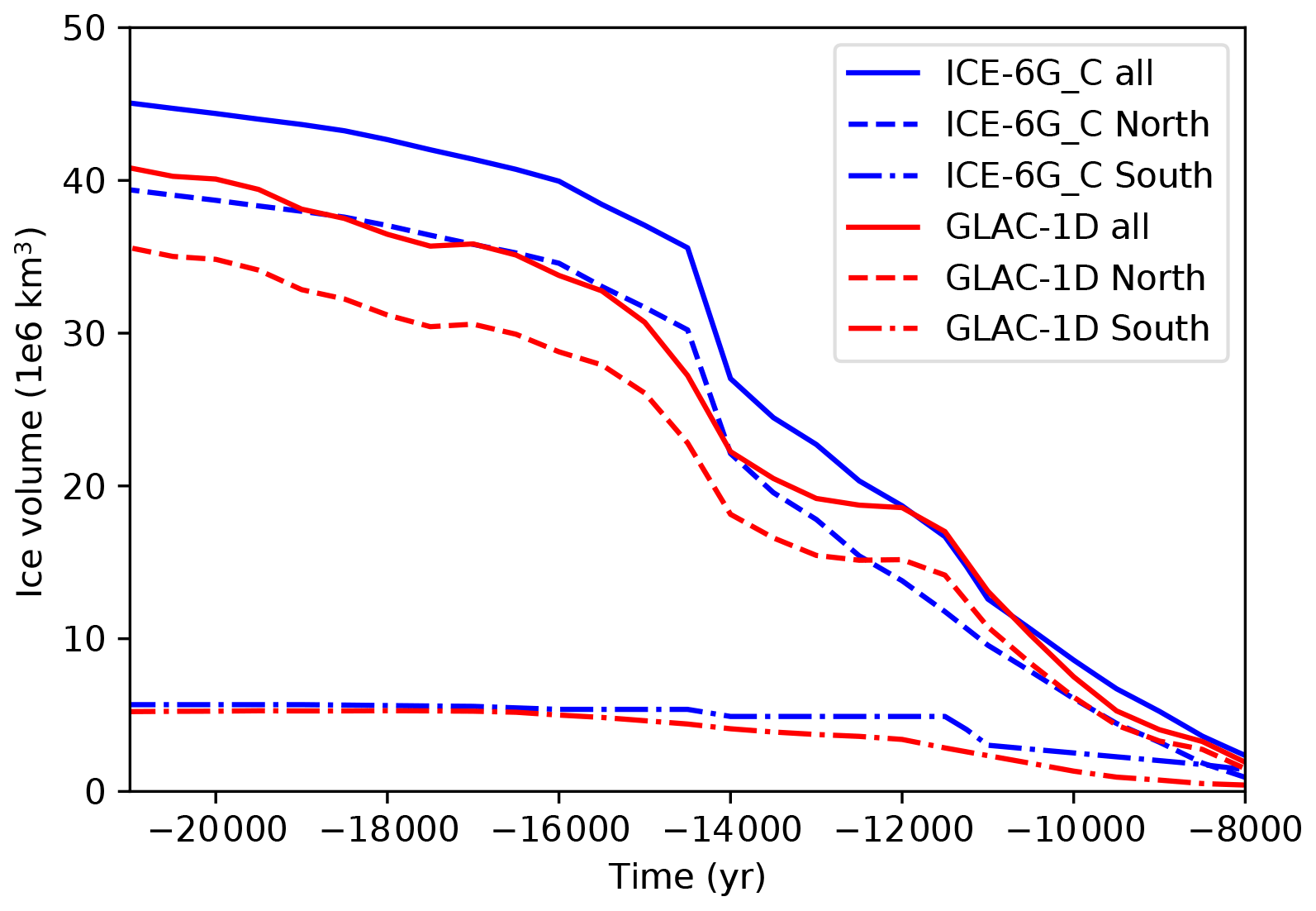
Figure 1Global ice sheet volume evolution (106 km3) for the two reconstructions (solid lines), with contributions of Northern Hemisphere (dashed lines) and Southern Hemisphere (dash-dotted lines) ice sheets (data from Ivanovic et al., 2016).
Besides the ice sheet reconstruction itself, the PMIP4 protocol lets the modelling group to some extent decide how to implement ice-sheet-related changes such as land–sea mask (i.e. coastlines), bathymetry and freshwater fluxes (FWFs). The purpose of this flexibility in the protocol is to allow any willing modelling group to join the effort, whatever the complexity of their model, from intermediate complexity to state-of-the art general circulation models (GCMs). However, not all models are able to run the entire range of possible simulations; it is thus crucial to evaluate the impact on climate of the different choices in setting up the experiments. More specifically, model groups have three choices related to ice sheets: (a) the choice of ice sheet reconstruction: ICE-6G_ C or GLAC-1D; (b) to only account for topography and ice mask (i.e. albedo changes) or also land–sea mask and bathymetry changes and (c) to account or not for the flux of meltwater from ice sheets to the ocean, and if included, to do so in a uniform way or a more realistic way such as by routing melted water towards the ocean. The relative effect of all these individual modelling choices on the transient climate simulations has not been evaluated.
The effect of ice-sheet-related changes has been analysed to some extent in past studies, but not all of them, usually not within the PMIP4 deglacial framework, and not in a systematic way. For example, an evolving bathymetry (including changes of coastlines) has recently been implemented in a GCM (Meccia and Mikolajewicz, 2018), and while it has been used in transient runs of the last deglaciation (Kapsch et al., 2022), the impact of evolving bathymetry compared to fixed bathymetry on climate has not been evaluated yet. Concerning freshwater fluxes, they were usually not included in early studies of deglacial changes (Timm and Timmermann, 2007; Roche et al., 2011; Smith and Gregory, 2012), possibly explaining the lack of rapid regional changes in these simulations. In contrast, in simulations with freshwater fluxes, rapid events were observed in addition to the global deglacial warming (Liu et al., 2009; Menviel et al., 2011; Bethke et al., 2012; He et al., 2013; Obase and Abe-Ouchi, 2019). However, the simulations that show temperature and circulation changes in best agreement with data were usually run with tuned freshwater fluxes (Liu et al., 2009; Menviel et al., 2011; He et al., 2013; Obase and Abe-Ouchi, 2019). On the one hand, such prescribed freshwater fluxes are usually inconsistent with the volume change inferred from ice sheet reconstructions. On the other hand, simulations run with the freshwater flux evolution derived from ice sheet reconstructions show disagreement with observed climate changes (e.g. Bethke et al., 2012; Kapsch et al., 2022).
Here, we evaluate the impact of ice-sheet-led changes, i.e. topography and albedo, bathymetry and coastlines, and freshwater fluxes, on climate, especially temperature and ocean circulation. For this, we use iLOVECLIM, a climate model of intermediate complexity, fast enough to run several simulations and test these different effects. This work will help other modelling groups decide which choices to make in terms of ice-sheet-related changes.
2.1 iLOVECLIM model
We use the iLOVECLIM model, which is a code fork and evolution of the LOVECLIM model (Goosse et al., 2010). The iLOVECLIM model is an intermediate complexity model which shares the same atmosphere, ocean, sea ice and terrestrial biosphere components as LOVECLIM. The ocean grid has a resolution with 20 irregular vertical levels, while the atmosphere is on a T21 grid with 3 vertical levels. It can simulate ∼1000 yr d−1, making it very suitable for computing long-term climate changes such as the work undertaken here.
To run simulations of the last deglaciation following the PMIP4 protocol, we have modified the code to be able to change the bathymetry and coastline regularly, and we have added the routing of freshwater from ice sheet melt to the ocean. We have also generated the ice sheet topography, ice sheet mask, bathymetry and land–sea mask files on the iLOVECLIM grid using the ICE-6G_C or GLAC-1D reconstructions. This is detailed in the sections below.
2.2 Modification of ice sheet topography and ice mask
The ice sheet geometry change is accounted for in the atmospheric component of the model through two variables: the surface elevation (topography) and the ice sheet mask (albedo). These two variables are updated interactively in the course of the simulation to follow the ICE-6G_C or GLAC-1D reconstructions, using anomalies with respect to ETOPO1 (NOAA National Geophysical Data Center, 2009). The updates are done abruptly, i.e. without temporal interpolation, every 500 years for the ICE-6G_C reconstruction and every 100 years for the GLAC-1D reconstruction. The difference in frequency update is due to the difference in the frequency of available ice sheet reconstructions (500 years for ICE-6G_C and every 100 years for GLAC-1D). The ice sheet albedo in the iLOVECLIM model is set to the constant and homogeneous value of 0.85. The vegetation is dynamically computed in the model by the terrestrial biosphere model (VECODE; Brovkin et al., 1997).
2.3 Modification of bathymetry and coastlines
We have extended the computation of bathymetry developed in Lhardy et al. (2021a) for the deglaciation. Following the same procedure, a new bathymetry has been adapted to the iLOVECLIM ocean grid based on those provided in the ICE-6G_C and GLAC-1D reconstructions at regular intervals starting at 21 ka. The bathymetry anomaly (with respect to the pre-industrial bathymetry) at each time step is added to the pre-industrial (PI) bathymetry based on ETOPO1. The bathymetry associated with each ice sheet reconstruction is interpolated into the ocean grid in an automated way, with a few limited manual adjustments in straits or key passages. We decide to maintain passages open at our grid resolution when they were open in the reconstructions. Since the ice sheet reconstruction (and thus bathymetry) is provided every 100 years for the GLAC-1D reconstruction and every 500 years for the ICE-6G_C reconstruction, we keep the same frequency for the bathymetry update in iLOVECLIM. To test the effect of the frequency update of bathymetry and land–sea mask, we have also run a simulation with GLAC-1D, updating the files every 500 years instead of every 100 years. With the reconstructed bathymetry, the ocean volume increases across the deglaciation due to the ice sheet volume decrease (Fig. 2). The initial volume of the ocean at the LGM is lower with ICE-6G_C (1.291×10¹⁸ m3) than with GLAC-1D (1.296×10¹⁸ m3) as more ice is stored in the ice sheets reconstructed with ICE-6G_C. Apart from this relatively constant shift, the evolution is rather similar in the two reconstructions until 14.5 ka. From around 14.5 ka, the ocean volume increase accelerates, and this acceleration is larger with ICE-6G_C so that the shift between both reconstructions is reduced. From around 12 ka and as we get nearer to the pre-industrial period, the ocean volume becomes roughly the same in both reconstructions: since the ice sheet topography is prescribed as an anomaly with respect to ETOPO1 in the model, when the additional ice sheet volume disappears, both ice sheet forcings converge.
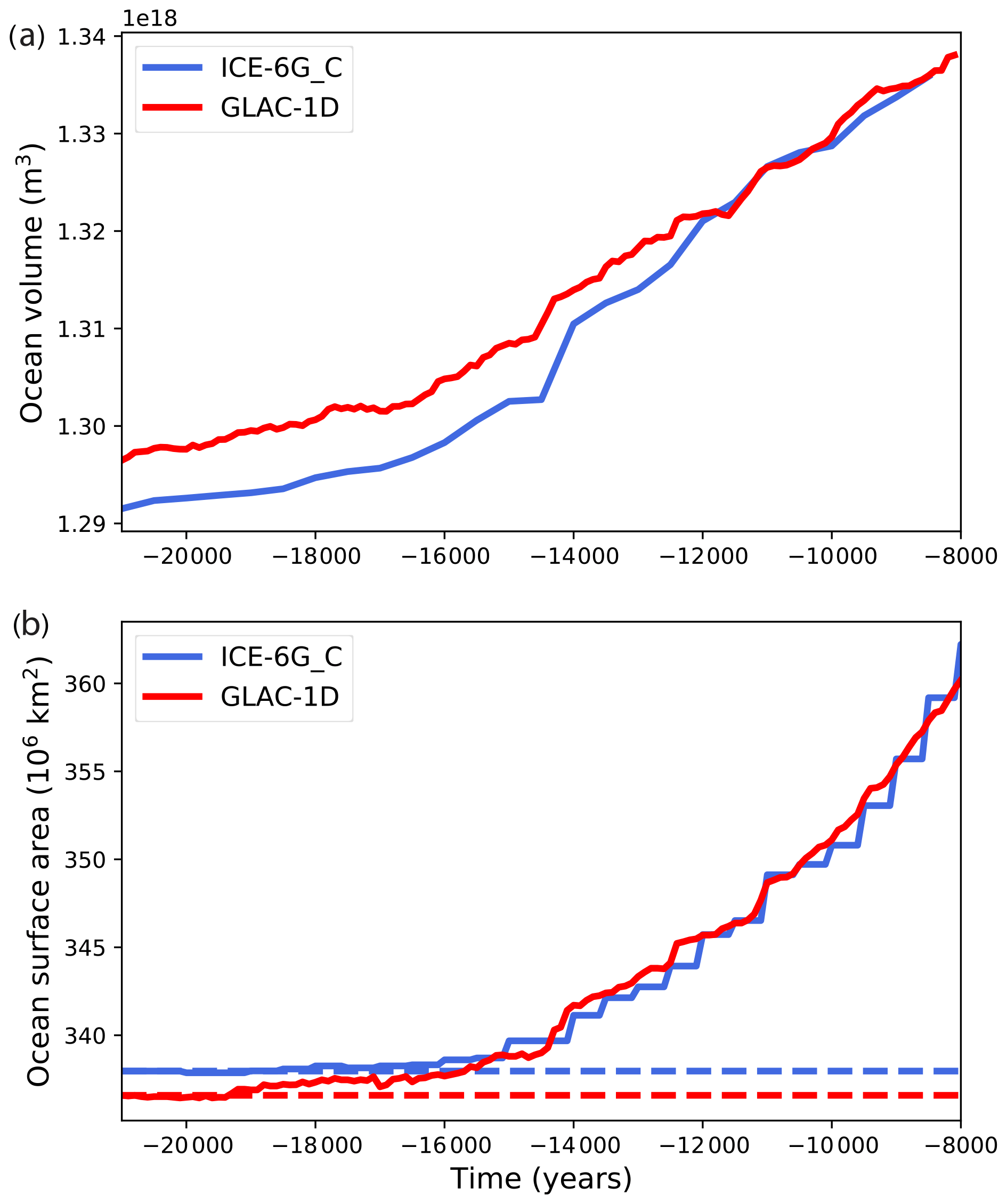
Figure 2Evolution of (a) the ocean volume (m3) with the ICE-6G_C and GLAC-1D bathymetry reconstructions and (b) the surface area (106 km2). The dashed lines indicate the values for the simulations with fixed bathymetry.
There is more variability in the GLAC-1D evolution due to the update of bathymetry every 100 years compared to every 500 years for ICE-6G. On top of that, from 12.5 ka, the evolution is more variable in GLAC-1D than in ICE-6G, with accelerations and slowdowns.
With the evolving bathymetry, we generate evolving land–sea masks (Fig. 3). At the LGM, the continental area is larger than at the pre-industrial bathymetry due to the lower sea level (Fig. 2b). It then decreases throughout the deglaciation while the sea level rises and new ocean grids appear. At the LGM, the new land–sea mask implies a closing of the Bering strait and Canadian archipelago. The strait of Gibraltar is maintained open throughout the simulation.
Every time the bathymetry is updated in the model, conservation of salt is ensured by redistributing the excess (or loss) of salt in the global ocean. In the new oceanic cells, the variables (such as temperature) are initialised using the mean value of neighbour cells. When new continent grids appear, the vegetation model computes a new albedo based on the vegetation distribution that is computed interactively by the model.
2.4 Routing of melted water from ice sheets
In iLOVECLIM, contrary to the original LOVECLIM model, the routing is no longer done in fixed routing basins. Rather, water routing is computed along the greater slope of the model topography and is updated accordingly whenever the topography is updated. This allows for a portable evolution of the first-order changes in river routing along the deglaciation. The routing is thus computed and used for the precipitation (interactive) and the anomalous freshwater flux arising from the ice sheet melt. The latter is computed as the change in ice sheet thickness between two reconstruction snapshots, averaged as an annual flux and applied homogeneously over the year. The water fluxes are added as a water flux into the ocean model, hence changing the salinity. With the new routing scheme, the freshwater flux from ice sheet melt is thus not added homogeneously in the ocean but routed towards the closest ocean grid cell following the topography.
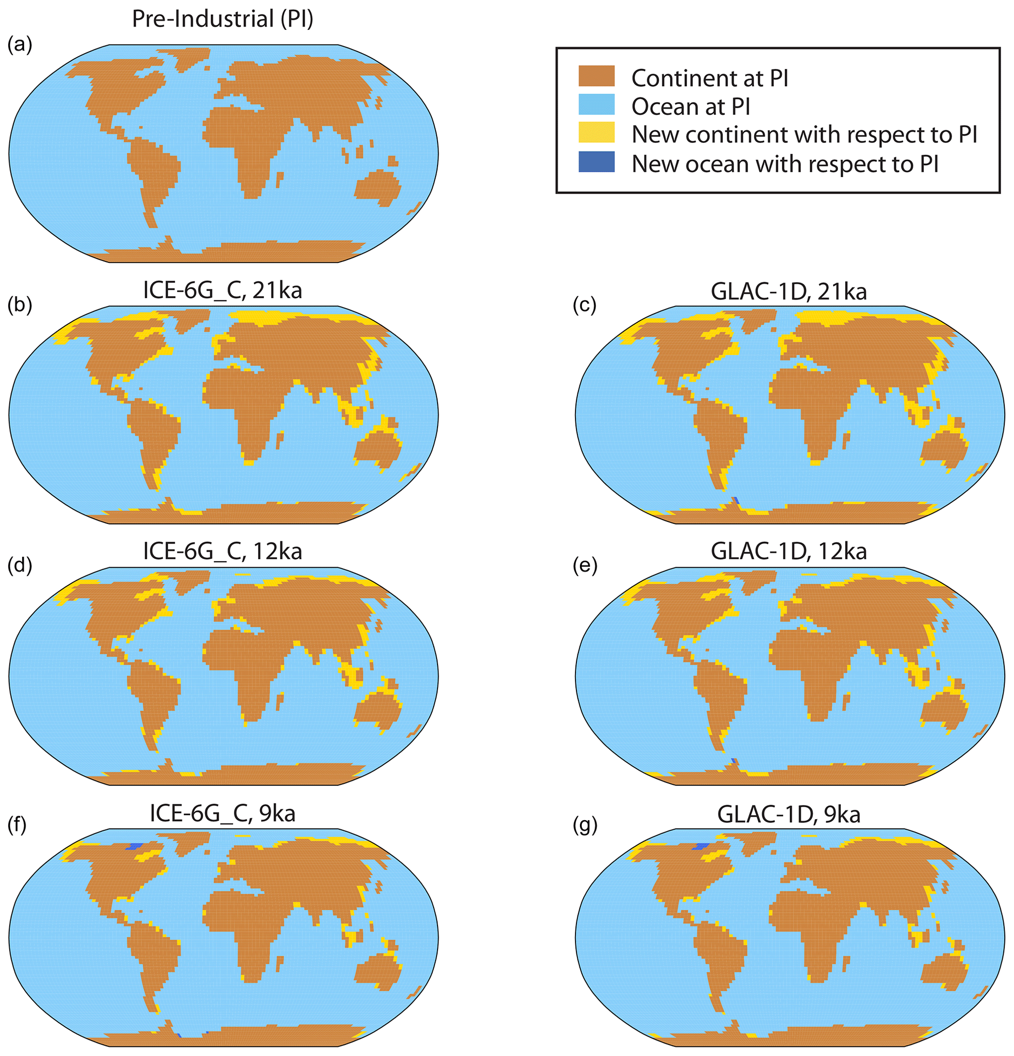
Figure 3Land–sea masks generated for the ICE-6G_C and GLAC-1D reconstructions.
2.5 Simulations following the PMIP4 protocol
All transient simulations are forced with evolving orbital parameters (Berger, 1978), as well as the increased concentration of greenhouse gases, notably CO2 (Bereiter et al., 2015), CH4 (Loulergue et al., 2008) and N2O (Schilt et al., 2010), following the PMIP4 deglacial protocol (Ivanovic et al., 2016). To evaluate the impact of ice-sheet-led changes, we have run a set of simulations (Table 1) in which we consider the following.
-
The role of ice sheet elevation and albedo: in the first two simulations, only the topography and albedo changes from ice sheets are accounted for, with the two different prescribed reconstructions – ICE-6G_C and GLAC-1D. In these simulations, the bathymetry and land–sea mask are fixed to the LGM ones.
-
The role of bathymetry: two simulations are run with the bathymetry and land–sea mask changes on top of topography changes for the two reconstructions.
-
The role of freshwater fluxes from ice sheet melting: a set of simulations with freshwater fluxes from the melting ice sheets are run for the GLAC-1D reconstruction.
The simulations are started from 5000-year-long spin-up runs with LGM conditions (GLAC-1D, ICE-6G), consistent with the deglaciation protocol.

3.1 Impact of different ice sheet reconstructions (topography and albedo)
The effects on climate of the two ice sheet reconstructions (ICE-6G_C and GLAC-1D) are first compared when only considering the changes of topography and albedo (no bathymetry nor freshwater changes). These simulations will serve as a reference for the other ones with the added effects of bathymetry and freshwater fluxes.
In both simulations, the global mean temperature is ∼4 ∘C colder at the LGM compared to the pre-industrial period (Fig. 4), in the range of the PMIP4 models' temperature change (3.3 to 7.2 ∘C; Kageyama et al., 2021) and reconstructions (Annan et al., 2022). The global mean temperature is slightly warmer in the simulation with the GLAC-1D reconstruction compared to the simulation with ICE-6G_C due to slightly smaller and lower ice sheets with GLAC-1D (Ivanovic et al., 2018; Fig. 1). This temperature difference is observed until ∼11.5 ka, when temperatures from both simulations reach similar values, due to the ice sheet volume evolution. Indeed, the ice sheet height and extent become similar for both reconstructions from ∼11.5 ka. The global mean temperature evolution is relatively similar to proxy data reconstruction (Shakun et al., 2012), with a progressive warming until ∼14 ka. At this time, while the data show a slowdown and then a decrease in temperature, the temperature with ICE-6G continues to increase while the temperature with GLAC-1D shows a stalling more similar to data, but at a later date. This can be linked to the Northern Hemisphere ice sheet reconstructions. In GLAC-1D, the ice volume decreases strongly until 14 ka, then stays constant from 14 to 12 ka. With ICE-6G_C, it continues to decrease, although at a lower rate. From ∼11 ka, both data and model simulations show an increase in temperature followed by a plateau at the beginning of the Holocene.
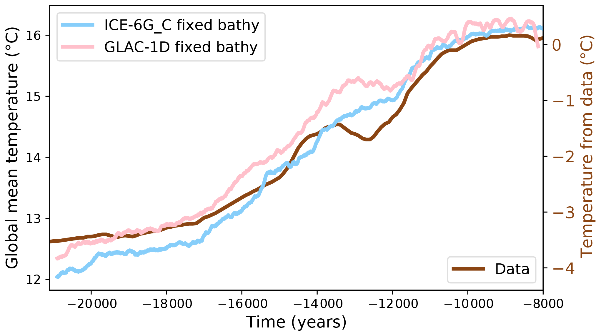
Figure 4Global mean annual temperature evolution (∘C) for the two simulations with the two ice sheet reconstructions (with fixed bathymetry and no freshwater flux), using the running mean over 100 years. The proxy data, which are shown as anomalies, are from Shakun et al. (2012).
The sea surface temperature distribution at the LGM and the warming pattern at the beginning of the Holocene at ∼8 ka compared to the LGM are also similar in the two simulations (Fig. 5a). Most of the warming at 10 ka has occurred in the North Atlantic and Southern Ocean, where deep water forms and penetrates in the ocean interior.
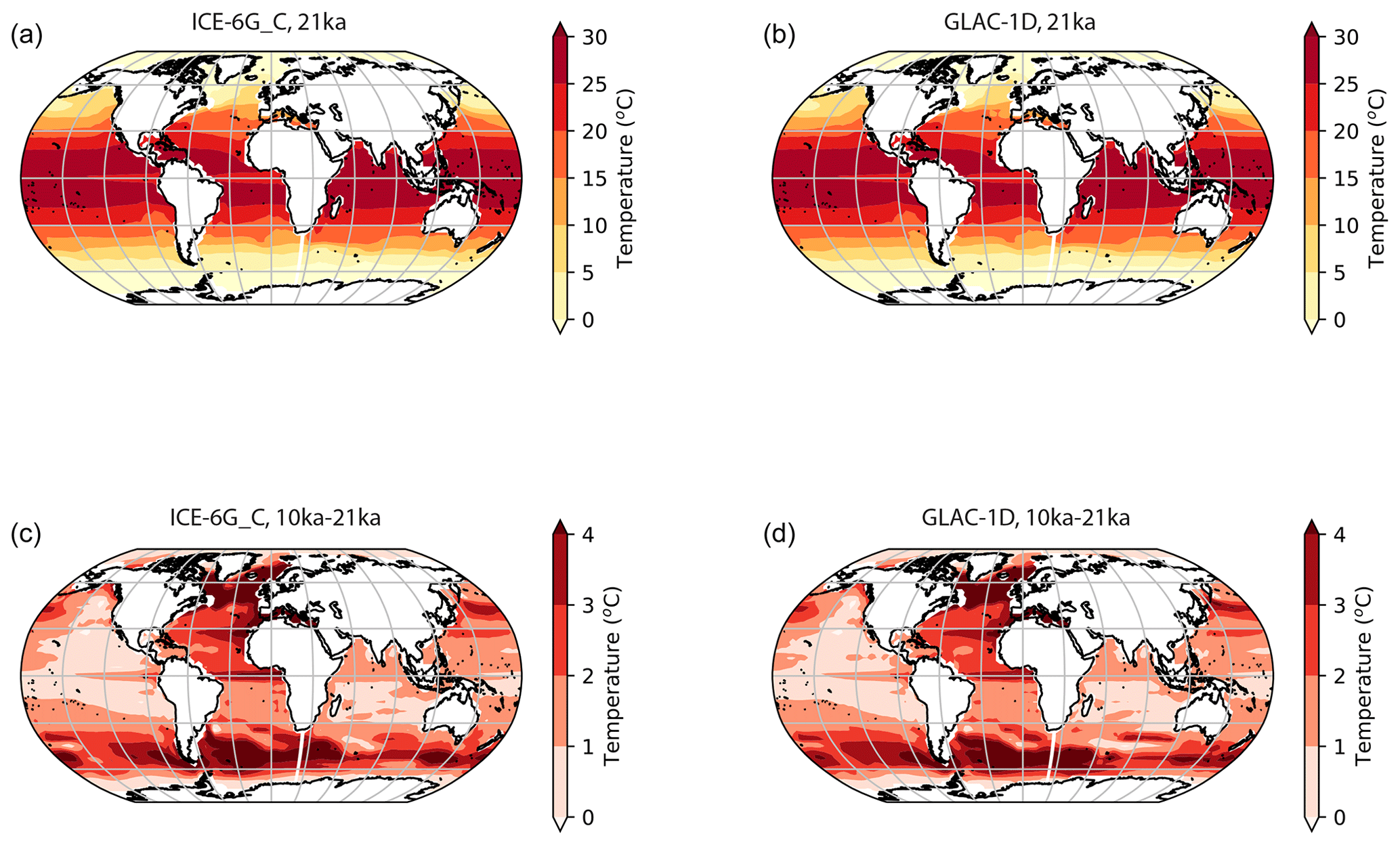
Figure 5Ocean sea surface temperature (∘C) at (a, b) 21 ka and (c, d) difference between 10 and 21 ka. The left panel is with ICE-6G_C and the right panel with GLAC-1D.
In summary, the first-order change of temperature is similar in the two simulations with the two reconstructions and in relatively good agreement with global mean data. The main differences are a temperature shift from 21 to 12 ka and a difference in the evolution between 14 and 12 ka at the time of the Antarctic Cold Reversal and Younger Dryas.
3.2 Impact of evolving bathymetry and land–sea mask (vs. fixed ones)
On top of the changes of topography and albedo, we have run simulations where we also modify the bathymetry and land–sea mask (later referred to as “with bathymetry”) for the two ice sheet reconstructions. The evolving bathymetry and land–sea mask lead to an increase of the ocean volume (Fig. 2), and hence a decrease of the global salinity as the global salt content is conserved (Fig. 6). The salinity change at the LGM that is computed directly from the volume change (1.4 psu for ICE-6G_C and 1.3 psu for GLAC-1D) is larger than the one prescribed in the PMIP4 standard protocol without bathymetry change where the bathymetry is fixed to the pre-industrial one (1 psu).
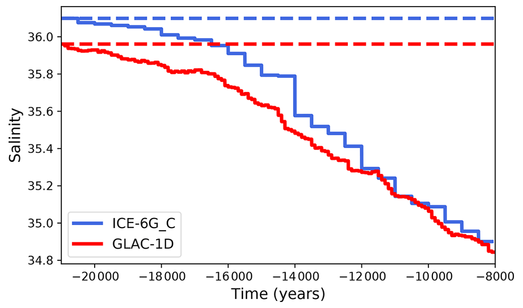
Figure 6Evolution of the global mean ocean salinity simulated in the model with the ICE-6G_C and GLAC-1D reconstructions. The dashed lines indicate the values for the simulations with fixed bathymetry.
Accounting for the progressive change of bathymetry over time due to the ice sheet changes has a limited impact on the global mean temperature: its evolution is relatively similar with or without accounting for bathymetry changes (Fig. 7a and b) apart from small changes, such as between 13 and 12 ka with ICE-6G, and a constant shift towards slightly colder temperatures from ∼12 ka onwards with ICE-6G_C and from ∼14 ka onwards with GLAC-1D.
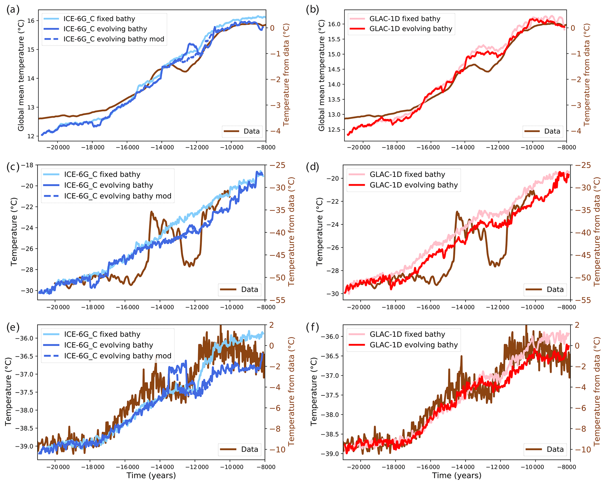
Figure 7Evolution of (a, b) global mean temperature (∘C), (c, d) temperature (∘C) at NGRIP (Greenland) and (e, f) temperature (∘C) at EDC (Antarctica). For the simulations, the left panels are with the ICE-6G_C reconstruction and the right ones with GLAC-1D. The simulated results are shown as the running mean over 100 years. Data are from Shakun et al. (2012), Buizert et al. (2014) and Jouzel et al. (2007). Note that the vertical scales for the model simulations (a, c, e) and for the measured data (b, d, f) are different.
The shift of temperature towards colder values is also visible in the temperature evolution in Greenland (Fig. 7c and d) and Antarctica (Fig. 7e and f). The relative cooling in the simulations with bathymetry changes compared to the simulations with fixed bathymetry is higher locally than at a global scale, especially in Greenland. The maximum cooling is ∼2 ∘C at the North Greenland Ice Core Project (NGRIP; 2.1 ∘C with ICE-6G_C and 2 ∘C with GLAC-1D) and ∼1 ∘C at EPICA Dome C (EDC; 1.1 ∘C with ICE-6G_C and 0.7 ∘C with GLAC-1D) compared to ∼0.4 ∘C globally (0.5 ∘C with ICE-6G_C and 0.3 ∘C with GLAC-1D). With both reconstructions, this shift is visible mostly from ∼14 ka onwards. With ICE-6G_C, Fig. 7e also shows a rapid increase then decrease of temperature between 14 and 12 ka in Antarctica. This is due to a change in the bathymetry and land–sea mask around Antarctica, where a grid cell switches from land to ocean. Forcing this grid cell to remain as land suppresses this unrealistic response (Fig. 7 simulation “ICE-6G_C evolving bathy mod”). In these simulations, there is no large abrupt climate change in Greenland contrary to data, as the AMOC strength remains strong throughout the simulation in the absence of freshwater flux (see “Discussion and conclusion” section and Fig. 14).
The shift towards colder temperature with evolving bathymetry is mainly due to the albedo change associated with the land–sea mask modification. As shown in Fig. 8, except for a few time periods, the albedo becomes higher in all simulations with evolving bathymetry compared to the corresponding simulations with fixed bathymetry, a difference that becomes more visible from ∼15–14 ka onward, at the same time as the shift in temperature observed in Fig. 7. In these simulations, the continental surface area decreases with time while the ocean expands due to the ice sheet volume decrease. While the ocean volume area starts changing earlier, the change in surface area only starts to be significant from ∼15 ka (Fig. 2). At high latitudes where it is cold enough to have sea ice, the continental surface whose albedo can vary from ∼0.1 without snow to ∼0.8 with snow is replaced by surfaces with sea ice, which has a high albedo of ∼0.8 (which can decrease depending on the sea ice type, down to 0.1 for very thin ice), leading to the cold temperatures.
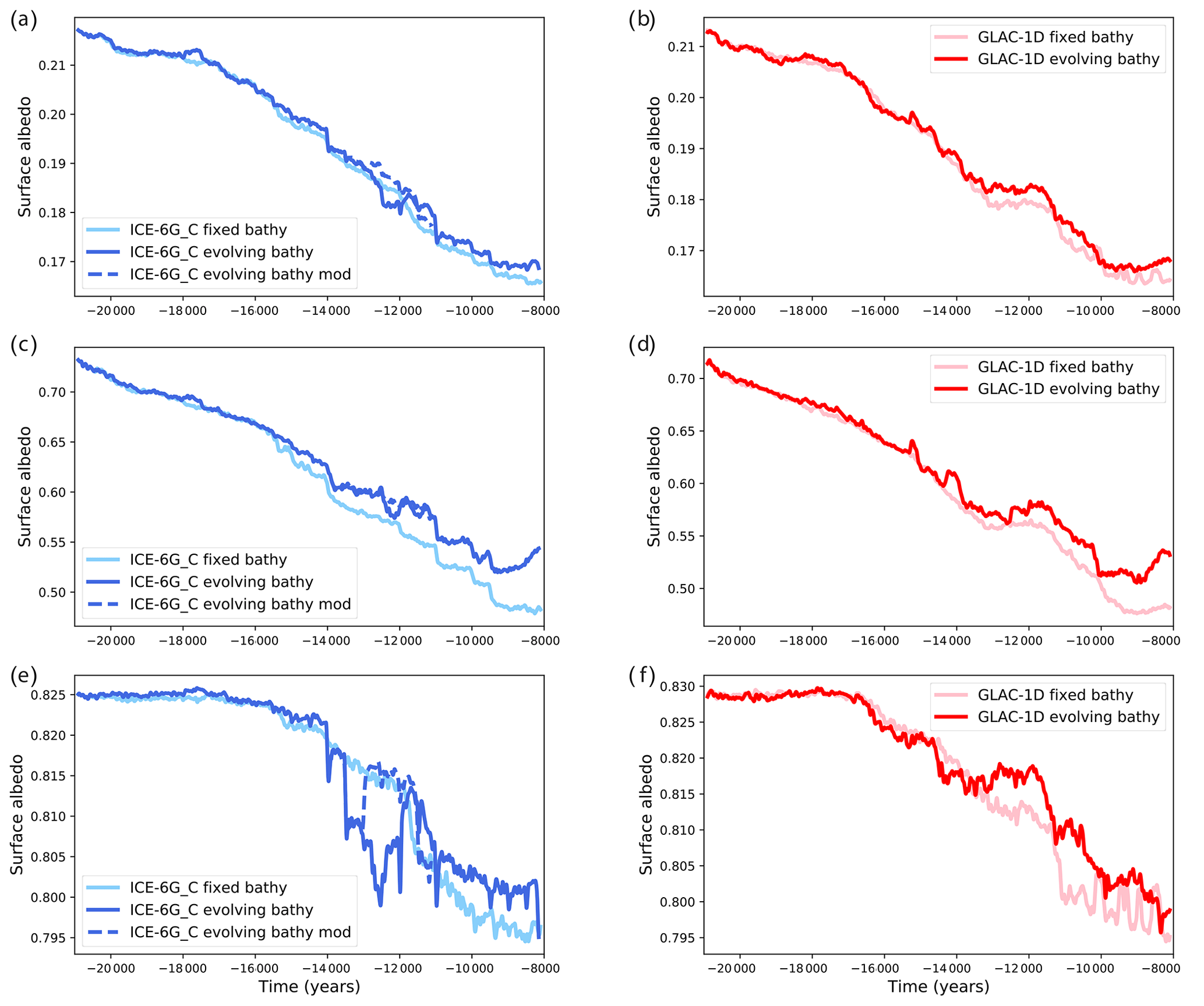
Figure 8Evolution of surface mean albedo over (a, b) the entire globe, (c, d) the Northern Hemisphere from 65 to 90∘ N and (e, f) the Southern Hemisphere from 90 to 65∘ S. Panels (a, c, e) are with the ICE-6G_C reconstruction and (b, d, f) with GLAC-1D.
In agreement with the albedo change, the sea ice area is also significantly impacted by the evolving bathymetry (Fig. 9), because the ocean surface area, especially in the North Atlantic and Arctic, but also in the Southern Ocean, is very different when accounting for bathymetry changes. Due to the sea level increase from ice sheet melt, the land–sea mask is modified, and the ocean surface in the high latitudes of the North Hemisphere increases with time, leaving more surface for sea ice to form where it is cold enough. From 15 ka onwards, this leads to more sea ice in the simulation with evolving bathymetry compared to the simulation with fixed bathymetry. With fixed bathymetry, the ocean surface is kept the same as the LGM one throughout the simulation (Fig. 2b), and the primary effect governing sea ice changes is the warming resulting in less area covered by sea ice over time. With evolving bathymetry, this effect is counteracted by the increase of ocean surface at high latitudes so that the sea ice area shows a more limited reduction.
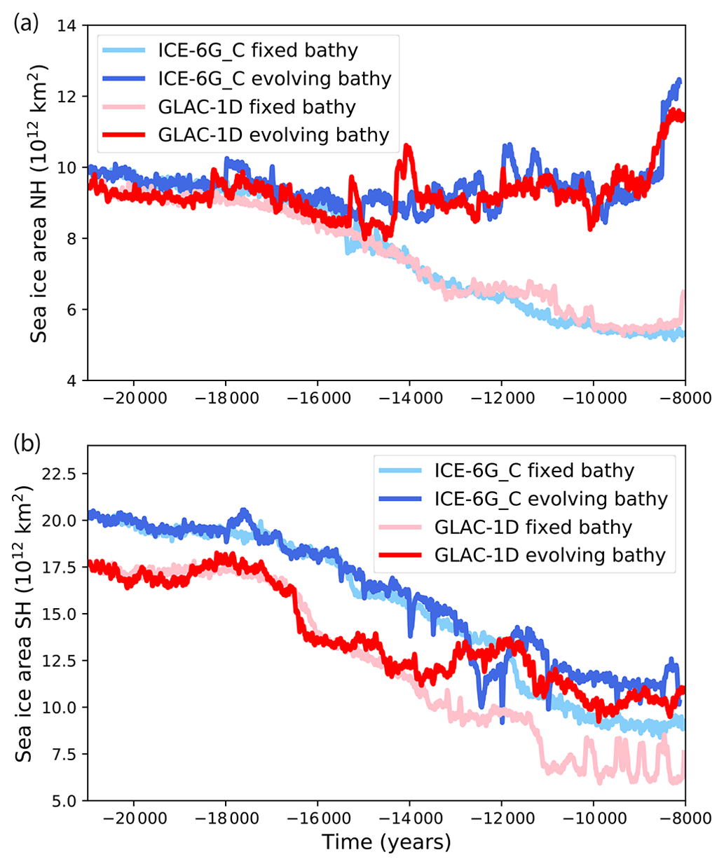
In the Southern Ocean, the land–sea mask changes less (Fig. 3) and later than in the North Atlantic, yielding apparent changes between simulations with and without bathymetry at a later date than in the Northern Hemisphere. The difference between simulations with and without bathymetry starts to be visible from 14 ka with GLAC-1D, and from 13 ka with ICE-6G. As can be seen in Fig. 1, the Antarctic ice sheet starts melting earlier with GLAC-1D compared to ICE-6G; we thus observe a stronger and earlier change in sea ice with the two GLAC-1D simulations than the ICE-6G simulations. With both reconstructions, apart from between 13 and 12 ka with ICE-6G, having an evolving bathymetry leads to a larger sea ice area compared to the simulation with fixed bathymetry, as the ocean surface where sea ice can form increases with evolving bathymetry.
The sea ice formation is tightly linked to convection and AMOC changes: the sea ice forms where it is cold enough for water to freeze, which corresponds to cold places where the water becomes denser. In the North Atlantic, deep convection occurs where the heat loss from the ocean to the atmosphere is large enough for the salty and warm water coming from the south to significantly cool and make the water dense enough to convect. The dominant effect of sea ice is to isolate the ocean from the atmosphere, preventing heat loss and hence convection, so that convection takes place at the sea ice edge where it is very cold and heat loss can take place. In the Southern Ocean, the dominant effect of sea ice is the release of brine (very salty water) during sea ice formation. This makes the water denser and favours convection.
At the LGM, due to the colder climate, the simulated Northern Hemisphere sea ice edge is shifted to the south with respect to the pre-industrial period with both ice sheet reconstructions (Fig. 10a and b), and the mixed layer depth is deep, showing strong convection in the Iceland, Norwegian and Irminger basins. At 10 ka, with the warmer conditions the sea ice edge retreats toward the north and the mixed layer depth is reduced in all simulations (Fig. 10). However, the convection sites differ between simulations. In particular, while there is a convection site in the Labrador Sea in the ICE-6G simulations with fixed bathymetry, this convection site is not visible anymore in the simulation with evolving bathymetry where the sea ice edge is shifted to the south. This is due to the colder conditions in the simulation with evolving bathymetry. The sea ice cover isolates the ocean from the atmosphere preventing cooling and deep convection from taking place in the Labrador Sea. Instead, another convection site is observed south of Greenland.

Figure 10Winter (DJF) mixed layer depth (m) and sea ice edge (defined by 15 % concentration) at different time steps in the fixed bathy and evolving bathy simulations, with the two reconstructions.
This difference in convection sites observed in the model (Renssen et al., 2005) could explain the strong change in AMOC strength in ICE-6G_C (Fig. 11a): the AMOC strength decreases from 12 ka when accounting for bathymetry change while it stays relatively constant with a fixed bathymetry, leading to a ∼10 Sv difference between the two simulations. This is not the case with GLAC-1D where only small changes between the two simulations can be seen. This can also be seen in the meridional streamfunction shown in Fig. 12. With evolving bathymetry and ICE-6G_C, the AMOC is weaker and shallower at 10 ka compared to the simulation with fixed bathymetry (with ICE-6G). In the GLAC-1D simulations, the sea ice edge and convection sites are also shifted southward in the simulation with evolving bathymetry compared to the one with fixed bathymetry (Fig. 10d and f), but the latitude change is smaller, and not sufficient to shut down the Labrador Sea convection site, hence it has a limited effect on the AMOC evolution compared to the ICE-6G_C simulations (Figs. 11 and 12).
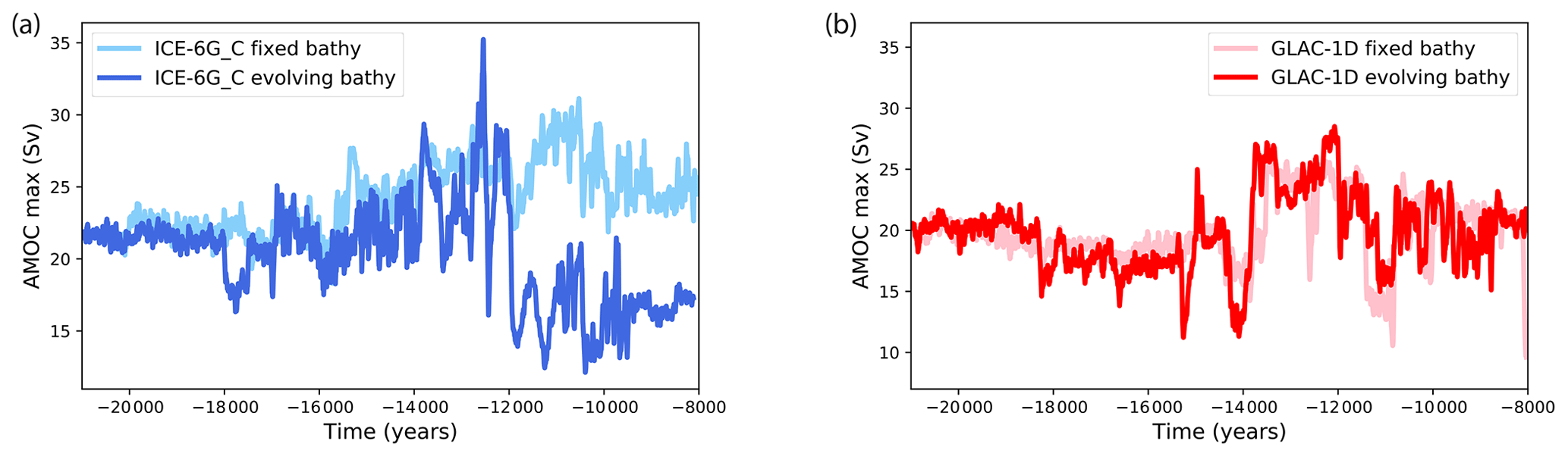
Figure 11Evolution of the maximum strength of the Atlantic meridional overturning circulation (Sv). Panel (a) is for the ICE-6G_C reconstruction and panel (b) for GLAC-1D. The simulated results are shown as the running mean over 100 years.
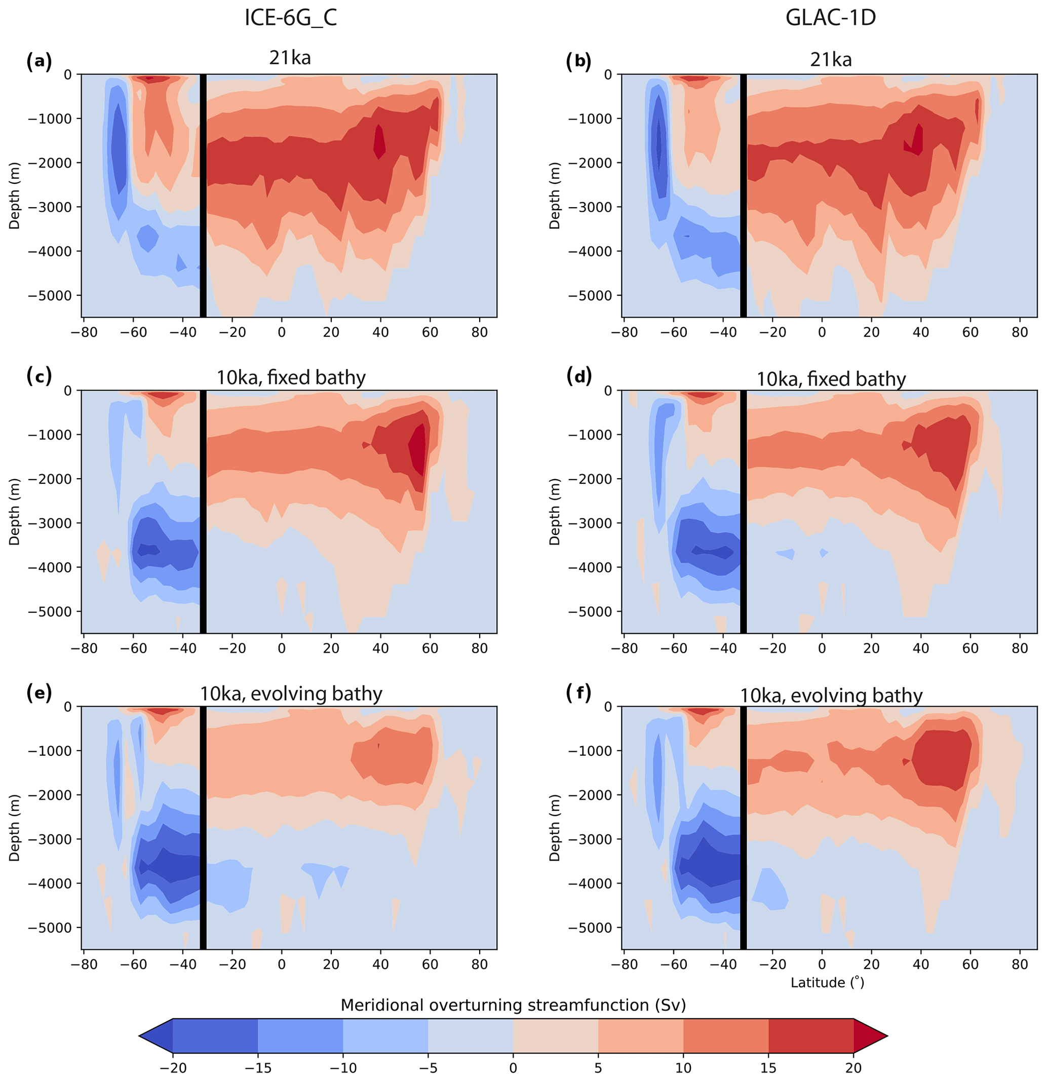
Figure 12Meridional overturning streamfunction (Sv) with the two reconstructions at different time steps, with fixed bathymetry and evolving bathymetry. The dark line indicates the limit between the Southern Ocean south of 32∘ S and the Atlantic Ocean north of 32∘ S.
The update frequency for bathymetry and land–sea mask is different for the two reconstructions: 500 years for ICE-6G_C and 100 years for GLAC-1D. To test the impact of different update frequency, we have run an additional simulation with the GLAC-1D reconstruction, with an update frequency of 500 years, similar to ICE-6G_C. As shown in Fig. 13, the frequency update modifies the global temperature evolution. It often results in a delayed response compared to the simulation with the 100-year frequency, as the bathymetry and land–sea mask change happens later, for example at ∼19, ∼16.5, ∼11 or ∼10 ka. Yet the effect is limited, and the difference between the two simulations with the same reconstruction but different update frequency is smaller than the difference between the simulations with the two reconstructions and the same update frequency.
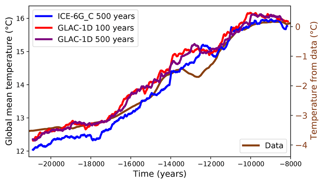
Figure 13Evolution of global mean temperature (∘C) for the simulations with evolving bathymetry with the ICE-6G_C or GLAC-1D reconstruction. For GLAC-1D, two update frequencies (100 and 500 years) have been tested. The simulated results are shown as the running mean over 100 years. Data are from Shakun et al. (2012). Note that the vertical scales for the model simulations (left) and for the measured data (right) are different.
In summary, accounting for bathymetry changes has limited impact on the global mean temperature change but can lead to large changes in regional climate, such as the convection sites, sea ice, AMOC and temperature in the North Atlantic. This depends on the reconstruction, the model grid resolution, and probably also on the model sensitivity.
3.3 Impact of freshwater flux from melting ice sheets
In addition to topography and bathymetry, changes of ice sheets can also have an impact on ocean circulation and climate through the input of freshwater coming from the melting of the ice. We now consider this impact by accounting for freshwater being routed from the site of ice sheet melting to the nearest ocean grid cell. The total water flux from ice sheet melting is relatively small (less than 0.1 Sv) until around 15 ka with both reconstructions (Fig. 14a). At 15 ka, the flux becomes very large, up to more than 0.5 Sv, corresponding to meltwater pulse 1A (Deschamps et al., 2012). After 14 ka, the fluxes from the two simulations differ more, with the flux from GLAC-1D showing more variability (due partly to the higher frequency update).
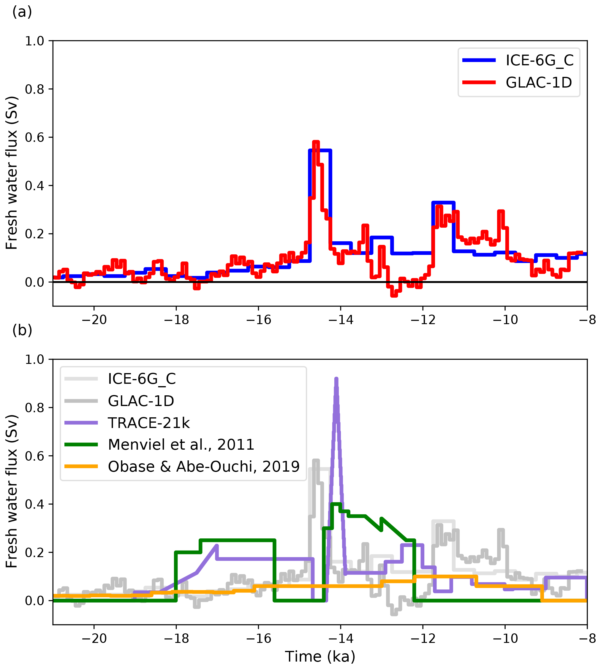
Figure 14Total freshwater flux (Sv) to the ocean due to ice sheet melting and comparison with other studies (Menviel et al., 2011; Obase and Abe-Ouchi, 2019). The values for TRACE-21k (Liu et al., 2009) have been obtained from https://www.cgd.ucar.edu/ccr/TraCE/TraCE.22,000.to.1950.overview.v2.htm (last access: 23 May 2023).
The freshwater input has a direct effect on convection as it reduces the surface salinity in convection zones, leading to reduced AMOC strength. This is the case with the FWF simulation showing a reduction of AMOC strength starting at around 15 ka (when the freshwater flux becomes very large), and a shutdown from around 14 ka (Fig. 15). In this simulation, the AMOC does not recover and the simulation crashes at year 11 792 BP, i.e. after 9208 years of simulations, for an unknown reason. The response to a freshwater flux is very model-dependent (Gottschalk et al., 2019). Hence, to emulate the response of a model less sensitive to freshwater inputs, we have reduced the flux by a factor of 3 and 4. With the reduction of a factor of 3 (), the AMOC still collapses and recovers only around 8 ka. With a larger factor of 4 (), the AMOC is weakened but quickly recovers. Similar changes of AMOC have been observed in an iLOVECLIM version coupled to an ice sheet model (Quiquet et al., 2021). As in other modelling studies using realistic freshwater fluxes computed from ice sheet melt (Kapsch et al., 2022), the timing of the AMOC weakening disagrees with data (McManus et al., 2004; Ng et al., 2018), taking place too late at around 15 ka when the freshwater flux becomes large, while proxy data indicate an AMOC weakening from ∼17 ka, when the freshwater flux is too small to have an impact on the simulated AMOC.
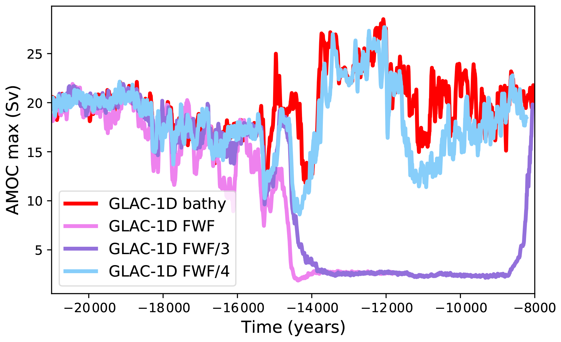
Figure 15Evolution of the maximum strength (Sv) of the Atlantic meridional overturning circulation (AMOC) for the simulations with freshwater fluxes.
Because of the AMOC reduction and shutdown, less heat is brought to the Northern Hemisphere and the temperatures in Greenland are strongly reduced in the FWF simulation compared to the standard simulation without FWF (Fig. 16b). This is also the case when the water flux is divided by 3. With the freshwater flux divided by 4 (), the AMOC strength is only slightly diminished, and the temperature decrease in Greenland is very limited, both in amplitude and in time as the AMOC recovers quickly. In this case, we observe two AMOC drops (Fig. 15, similar to those observed in Kapsch et al., 2022), and simultaneously two temperature drops in the Greenland temperature evolution (Fig. 16b).
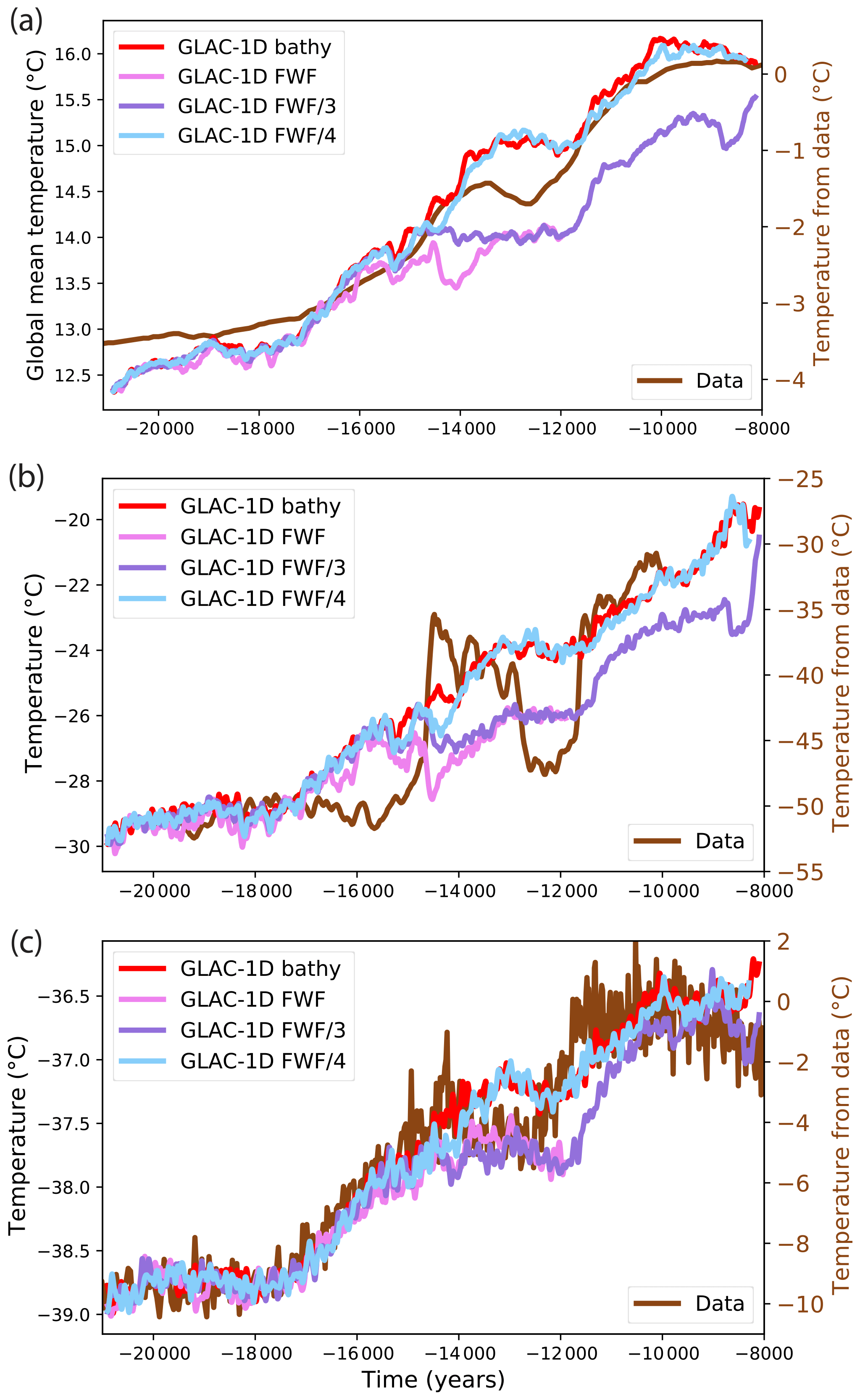
Figure 16Temperature evolution (∘C) for the simulations with freshwater fluxes (a) of the global mean (b) at NGRIP (Greenland) and (c) at EDC (Antarctica). The simulated results are shown as the running mean over 100 years and compared to proxy data (Shakun et al., 2012; Buizert et al., 2014; Jouzel et al., 2007).
While the Bolling–Allerod warming in the Greenland record at ∼14.5 ka cannot be simulated in the GLAC-1D FWF due to the freshwater flux from ice sheet melting becoming substantial only later at ∼15 ka, the temperature evolution in Antarctica and in the global mean (Fig. 16a and c) is in better agreement in the model compared to data, with a stalling in the temperature increase at the time of the Antarctic Cold Reversal from ∼14.5 ka. Yet the warming that starts again at ∼12 ka in the data lags in the simulations with FWF.
Using the iLOVECLIM model of intermediate complexity, we have evaluated the impact of different ice sheet reconstructions, separating their different effects: the change of topography (and albedo), the change of bathymetry (and land–sea mask) and the change of freshwater fluxes from the ice sheet melt.
4.1 Different ice sheet reconstructions
In our simulations, the ice sheets are prescribed based on two reconstructions: ICE-6G_C and GLAC-1D, following the PMIP4 protocol. We show that the two reconstructions result in differences in terms of amplitude and timing of climate changes. In particular, the global mean temperature is ∼0.3 ∘C warmer with GLAC-1D compared to the simulation with ICE-6_C from the LGM to ∼12 ka. Between 14 and 12 ka, the evolution between the two simulations differ. Only the simulation with GLAC-1D displays a stalling in the temperature warming similar to data, albeit with a lag compared to data.
4.2 Bathymetry
In most past studies of deglacial simulation, the bathymetry was fixed, either at the LGM or the PI. We have shown here that the impact of accounting for bathymetric changes is a shift towards colder values, which is relatively limited for global mean temperature but more important regionally. This effect is mainly due to the different albedo with and without bathymetry changes. With evolving bathymetry, some grid cells are progressively changed from continent to ocean throughout the deglaciation, increasing the space available in the Nordic Seas especially. This results in a larger sea ice area with a higher albedo, which cools the climate and modifies the convection zones in the North Atlantic. As we demonstrate that bathymetry changes can impact the local and global climate, we advise to account for them (when technically possible) in deglacial simulations. However, changes of bathymetry can also trigger unrealistic changes, such as observed here in the simulations with the ICE-6G_C reconstruction at ∼13.5 ka around Antarctica. Using a higher resolution might help, but this shows that accounting for realistic bathymetry changes remains challenging.
The evolution of bathymetry depends on the ice sheet reconstructions. As the reconstructions are improved over time, the bathymetry change will also become more constrained. However, the model grid change resulting from the bathymetry change is not always straightforward when seaways become small and especially smaller than the grid cells: should a passage stay open in the model even if it results in a larger seaway, or should it be closed, even though it is not completely closed in the reconstructions? In this study, we have chosen to keep seaways open when they were open in the reconstructions, even if they were smaller than the grid cells. Yet, it would be interesting to test the impact of closing them. This issue is related to the model resolution: with higher-resolution models, it is possible to keep small seaways open, while in lower-resolution models, the grid cells are sometimes too large. In addition, we have chosen to keep the frequency of bathymetry update from the original frequency of the ice sheet reconstructions. This results in two different frequencies for the two reconstructions (500 and 100 years). Testing the impact of different update frequencies for the same reconstructions show some limited impact: a less frequent update leads to delays in the climate response as the changes take place later. Yet this effect is small compared to the change in climate from the two different reconstructions with the same update frequency.
In LGM simulations, a previous study showed that accounting for bathymetry and land–sea mask change was crucial for the carbon cycle (Lhardy et al., 2021b). A change of bathymetry, especially the one associated ocean volume change, modifies the ocean carbon storage capacity. As it is a very large carbon reservoir compared to the atmosphere, even changes of around 3 %, the order of magnitude between LGM and PI volume changes, can largely impact atmospheric CO2. This effect remains to be tested for the deglaciation.
In our study, the ice sheets are prescribed from reconstructions. In reality, ice sheets and climate interact. While the use of prescribed ice sheets is a limitation of this study, this topic has been addressed in Quiquet et al. (2021) with an interactive ice sheet model coupled to the iLOVECLIM model. These simulations show similar results in terms of temperature and ocean circulation changes. However, the bathymetry was fixed in such simulations. As shown here, the regional temperature can be impacted by the changes of bathymetry, which influences oceanic circulation and hence the transport of heat. In the simulations with evolving bathymetry, the temperature is colder over Greenland and Antarctica compared to the simulation with fixed bathymetry (Fig. 7). In simulations with interactive ice sheets, this would impact the mass balance and could lead to a different evolution of ice sheets.
4.3 Freshwater fluxes
In iLOVECLIM, the AMOC is very sensitive to the freshwater flux, resulting in an AMOC shutdown when freshwater input from ice sheet melting is included. The AMOC then remains in this collapsed state for several thousand years. The sensitivity to freshwater flux is very model-dependent (Gottschalk et al., 2019), and some other models display less sensitivity. For example, with the MPI-ESM model (Kapsch et al., 2022), the same freshwater fluxes computed from the ice sheet melt from the ICE-6G_C and GLAC-1D reconstructions result in weaker AMOC but no collapse, more similar to our simulation. In a simulation with HadCM3, a larger sensitivity of AMOC to the freshwater flux is obtained, but only for the 19 to 16 ka period as the simulation was not continued after that (Ivanovic et al., 2018).
In most past studies of deglacial simulations (apart from Kapsch et al., 2022 and Ivanovic et al., 2018), freshwater fluxes were prescribed and not computed from the ice sheet melting. In addition, in most previous studies, the areas where freshwater flux is added are prescribed. In this study, the freshwater flux is computed from the ice sheet volume change and routed towards the ocean following the topography. In Fig. 14, we compare the freshwater fluxes used in those simulations. In most model studies, the freshwater flux is much smaller and/or with a different timing compared to the ones computed from the ICE-6G_C and GLAC-1D reconstructions. This leads to a smaller evolution of sea level equivalent than in the reconstructions (Fig. 17). These models obtained a similar evolution of AMOC compared to proxy data and accordingly a relatively good evolution of temperature in Greenland, but the prescribed freshwater flux is in disagreement with the currently available ice sheet reconstructions. It is noteworthy that while in most models, freshwater fluxes are necessary to trigger large ocean circulation changes, one model has displayed changes in ocean circulation without freshwater fluxes (Zhu et al., 2014). In this simulation, the ocean circulation change was due to the orographic change of the ice sheet only (Zhu et al., 2014). However, the prescribed freshwater fluxes are also smaller than in the reconstruction, leading to smaller sea level change compared to data. Larger freshwater fluxes similar to the data may lead to different and possibly degraded results compared to data.
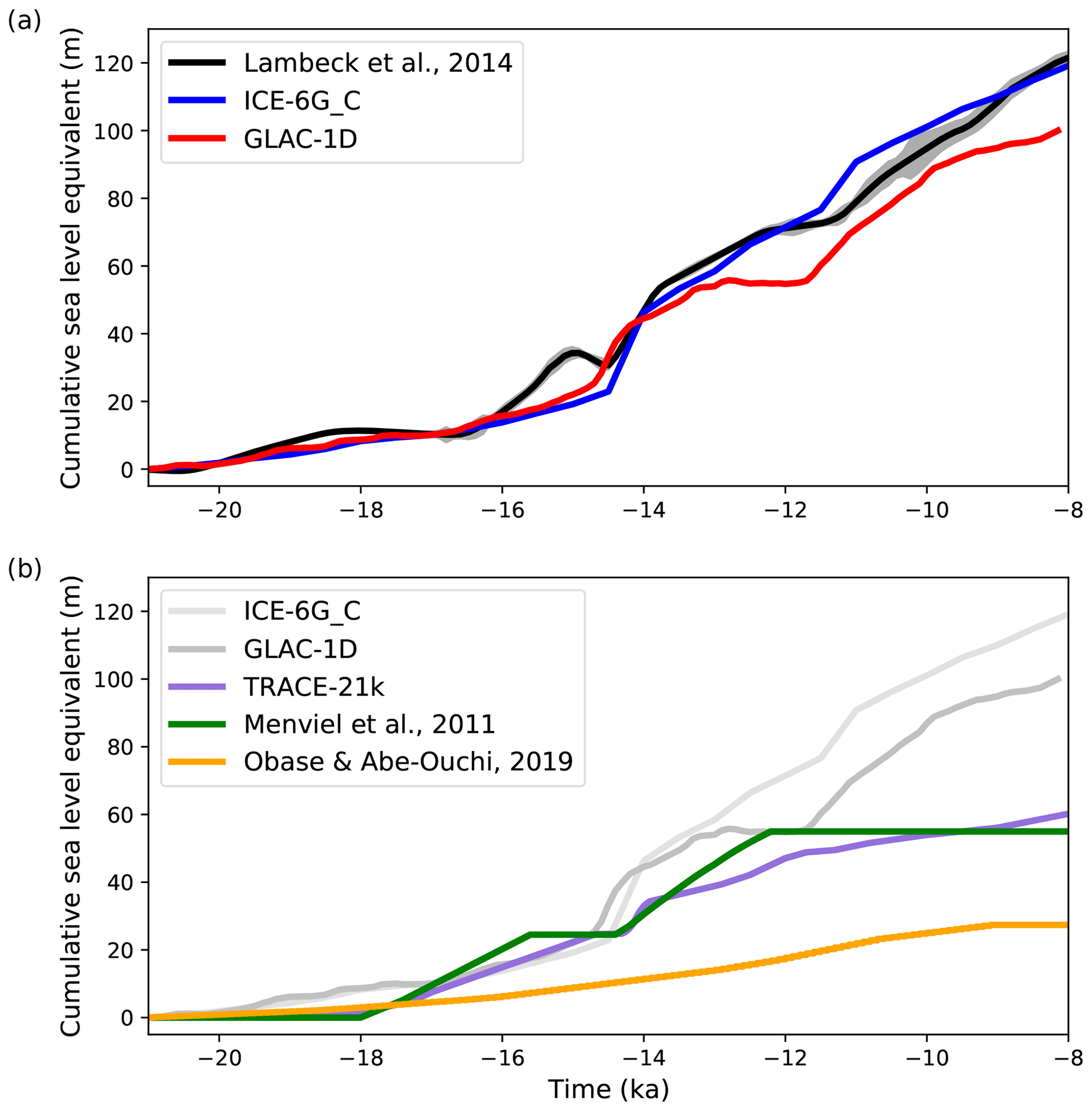
Figure 17Equivalent sea level evolution (m) due to the freshwater input (displayed in Fig. 14).
It is thus difficult for models to explain the large change of ocean circulation and the related change of temperature in the Northern and Southern hemispheres between 18 and 15 ka by freshwater fluxes. Either the ice sheet and sea level reconstructions should be revisited, the modelled AMOC sensitivity modified, or other processes explaining the AMOC change need to be tested.
The source data of the figures presented in the main text of the paper are available on the Zenodo repository with https://doi.org/10.5281/zenodo.7857361 (Bouttes et al., 2023).
NB, FL, DR and DP developed the model code for bathymetry changes. NB, AQ and DR developed the model code for freshwater fluxes. NB performed the simulations. NB analysed the results and prepared the figures. NB wrote the manuscript with contributions from all co-authors.
The contact author has declared that none of the authors has any competing interests.
Publisher's note: Copernicus Publications remains neutral with regard to jurisdictional claims in published maps and institutional affiliations.
We are thankful to two anonymous reviewers for their comments, which helped improve this paper.
This research has been supported by the French National Programme LEFE (Les Enveloppes Fluides et l'Environnement).
This paper was edited by Erin McClymont and reviewed by two anonymous referees.
Annan, J. D., Hargreaves, J. C., and Mauritsen, T.: A new global surface temperature reconstruction for the Last Glacial Maximum, Clim. Past, 18, 1883–1896, https://doi.org/10.5194/cp-18-1883-2022, 2022.
Argus, D. F., Peltier, W. R., Drummond, R., and Moore, A. W.: The Antarctica component of postglacial rebound model ICE-6G_C (VM5a) based on GPS positioning, exposure age dating of ice thicknesses, and relative sea level histories, Geophys. J. Int., 198, 537–563, https://doi.org/10.1093/gji/ggu140, 2014.
Bereiter, B., Eggleston, S., Schmitt, J., Nehrbass-Ahles, C., Stocker, T. F., Fischer, H., Kipfstuhl, S., and Chappellaz, J.: Revision of the EPICA Dome C CO2 record from 800 to 600 kyr before present, Geophys. Res. Lett., 42, 542–549, https://doi.org/10.1002/2014GL061957, 2015.
Berger, A.: Long-Term Variations of Daily Insolation and Quaternary Climatic Changes, J. Atmos. Sci., 35, 2362–2367, https://doi.org/10.1175/1520-0469(1978)035<2362:LTVODI>2.0.CO;2, 1978.
Bethke, I., Li, C., and Nisancioglu, K. H.: Can we use ice sheet reconstructions to constrain meltwater for deglacial simulations?, Paleoceanography, 27, PA2205, https://doi.org/10.1029/2011PA002258, 2012.
Bonelli, S., Charbit, S., Kageyama, M., Woillez, M.-N., Ramstein, G., Dumas, C., and Quiquet, A.: Investigating the evolution of major Northern Hemisphere ice sheets during the last glacialinterglacial cycle, Clim. Past, 5, 329–345, https://doi.org/10.5194/cp-5-329-2009, 2009.
Bouttes, N., Lhardy, F., Quiquet, A., Paillard, D., Goosse, H., and Roche, D. M.: Deglacial climate changes as forced by different ice sheet reconstructions – model ouputs, Zenodo [code], https://doi.org/10.5281/zenodo.7857361, 2023.
Briggs, R. D., Pollard, D., and Tarasov, L.: A data constrained large ensemble analysis of Antarctic evolution since the Eemian, Quaternary Sci. Rev., 103, 91–115, https://doi.org/10.1016/j.quascirev.2014.09.003, 2014.
Brovkin, V., Ganopolski, A., and Svirezhev, Y.: A continuous climate-vegetation classification for use in climate-biosphere studies, Ecol. Model., 101, 251–261, 1997.
Buizert, C., Gkinis, V., Severinghaus, J. P., He, F., Lecavalier, B. S., Kindler, P., Leuenberger, M., Carlson, A. E., Vinther, B., Masson-Delmotte, V., White, J. W. C., Liu, Z., Otto-Bliesner, B., and Brook, E. J.: Greenland temperature response to climate forcing during the last deglaciation, Science, 345, 1177–1180, https://doi.org/10.1126/science.1254961, 2014.
Clark, P. U., Shakun, J. D., Baker, P. A., Bartlein, P. J., Brewer, S., Brook, E., Carlson, A. E., Cheng, H., Kaufman, D. S., Liu, Z., Marchitto, T. M., Mix, A. C., Morrill, C., Otto-Bliesner, B. L., Pahnke, K., Russell, J. M., Whitlock, C., Adkins, J. F., Blois, J. L., Clark, J., Colman, S. M., Curry, W. B., Flower, B. P., He, F., Johnson, T. C., Lynch-Stieglitz, J., Markgraf, V., McManus, J., Mitrovica, J. X., Moreno, P. I., and Williams, J. W.: Global climate evolution during the last deglaciation, P. Natl. Acad. Sci. USA, 109, E1134–E1142, https://doi.org/10.1073/pnas.1116619109, 2012.
Deschamps, P., Durand, N., Bard, E., Hamelin, B., Camoin, G., Thomas, A. L., Henderson, G. M., Okuno, J., and Yokoyama, Y.: Ice-sheet collapse and sea-level rise at the Bølling warming 14,600 years ago, Nature, 28, 559–564, https://doi.org/10.1038/nature10902, 2012.
Ganopolski, A., Calov, R., and Claussen, M.: Simulation of the last glacial cycle with a coupled climate ice-sheet model of intermediate complexity, Clim. Past, 6, 229–244, https://doi.org/10.5194/cp-6-229-2010, 2010.
Goosse, H., Brovkin, V., Fichefet, T., Haarsma, R., Huybrechts, P., Jongma, J., Mouchet, A., Selten, F., Barriat, P.-Y., Campin, J.-M., Deleersnijder, E., Driesschaert, E., Goelzer, H., Janssens, I., Loutre, M.-F., Morales Maqueda, M. A., Opsteegh, T., Mathieu, P.-P., Munhoven, G., Pettersson, E. J., Renssen, H., Roche, D. M., Schaeffer, M., Tartinville, B., Timmermann, A., and Weber, S. L.: Description of the Earth system model of intermediate complexity LOVECLIM version 1.2, Geosci. Model Dev., 3, 603–633, https://doi.org/10.5194/gmd-3-603-2010, 2010.
Gottschalk, J., Battaglia, G., Fischer, H., Frölicher, T. L., Haccard, S. L., Jeltsch-Thömmes, A., Joos, F., Köhler, P., Meissner, K. J., Menviel, L., Nehrbass-Ahles, C., Schmitt, J., Schmittner, A., Skinner, L. C., and Stocker, T. F.: Mechanisms of millennial-scale atmospheric CO2 change in numerical model simulations, Quaternary Sci. Rev., 220, 30–74, https://doi.org/10.1016/j.quascirev.2019.05.013, 2019.
Gowan, E. J., Zhang, X., Khosravi, S., Rovere, A., Stocchi, P., Hughes, A. L. C., Gyllencreutz, R., Mangerud, J., Svendsen, J.-I., and Lohmann, G.: A new global ice sheet reconstruction for the past 80 000 years, Nat. Commun., 12, 1199, https://doi.org/10.1038/s41467-021-21469-w, 2021.
Gregoire, L. J., Valdes, P. J., and Payne, A. J.: The relative contribution of orbital forcing and greenhouse gases to the North American deglaciation, Geophys. Res. Lett., 42, 9970–9979, https://doi.org/10.1002/2015GL066005, 2015.
He, F., Shakun, J. D., Clark, P. U., Carlson, A. E., Liu, Z., Otto-Bliesner, B. L., and Kutzbach, J. E.: Northern Hemisphere forcing of Southern Hemisphere climate during the last deglaciation, Nature, 494, 81–85, https://doi.org/10.1038/nature11822, 2013.
Ivanovic, R. F., Gregoire, L. J., Kageyama, M., Roche, D. M., Valdes, P. J., Burke, A., Drummond, R., Peltier, W. R., and Tarasov, L.: Transient climate simulations of the deglaciation 21–9 thousand years before present (version 1) – PMIP4 Core experiment design and boundary conditions, Geosci. Model Dev., 9, 2563–2587, https://doi.org/10.5194/gmd-9-2563-2016, 2016.
Ivanovic, R. F., Gregoire, L. J., Burke, A., Wickert, A. D., Valdes, P. J., Ng, H. C., Robinson, L. F., McManus, J. F., Mitrovica, J. X., Lee, L., and Dentith, J. E.: Acceleration of northern ice sheet melt induces AMOC slowdown and northern cooling in simulations of the early last deglaciation, Paleoceanogr. Paleocl., 33, 807–824, https://doi.org/10.1029/2017PA003308, 2018.
Jouzel, J., Masson-Delmotte, V., Cattani, O., Dreyfus, G., Falourd, S., Hoffmann, G., Minster, B., Nouet, J., Barnola, J. M., Chappellaz, J., Fischer, H., Gallet, J. C., Johnsen, S., Leuenberger, M., Loulergue, L., Luethi, D., Oerter, H., Parrenin, F., Raisbeck, G., Raynaud, D., Schilt, A., Schwander, J., Selmo, E., Souchez, R., Spahni, R., Stauffer, B., Steffensen, J. P., Stenni, B., Stocker, T. F., Tison, J. L., Werner, M., and Wolff, E. W.: Orbital and Millennial Antarctic Climate Variability over the Past 800 000 Years, Science, 317, 793–796, https://doi.org/10.1126/science.1141038, 2007.
Kageyama, M., Harrison, S. P., Kapsch, M.-L., Lofverstrom, M., Lora, J. M., Mikolajewicz, U., Sherriff-Tadano, S., Vadsaria, T., Abe-Ouchi, A., Bouttes, N., Chandan, D., Gregoire, L. J., Ivanovic, R. F., Izumi, K., LeGrande, A. N., Lhardy, F., Lohmann, G., Morozova, P. A., Ohgaito, R., Paul, A., Peltier, W. R., Poulsen, C. J., Quiquet, A., Roche, D. M., Shi, X., Tierney, J. E., Valdes, P. J., Volodin, E., and Zhu, J.: The PMIP4 Last Glacial Maximum experiments: preliminary results and comparison with the PMIP3 simulations, Clim. Past, 17, 1065–1089, https://doi.org/10.5194/cp-17-1065-2021, 2021.
Kapsch, M.-L., Mikolajewicz, U., Ziemen, F., and Schannwell, C.: Ocean response in transient simulations of the last deglaciation dominated by underlying ice-sheet reconstruction and method of meltwater distribution, Geophys. Res. Lett., 49, e2021GL096767, https://doi.org/10.1029/2021GL096767, 2022.
Lambeck, K., Rouby, H., Purcell, A., Sun, Y., and Sambridge, M.: Sea level and global ice volumes from the Last Glacial Maximum to the Holocene, P. Natl. Acad. Sci. USA, 111, 15296–15303, https://doi.org/10.1073/pnas.1411762111, 2014.
Lhardy, F., Bouttes, N., Roche, D. M., Crosta, X., Waelbroeck, C., and Paillard, D.: Impact of Southern Ocean surface conditions on deep ocean circulation during the LGM: a model analysis, Clim. Past, 17, 1139–1159, https://doi.org/10.5194/cp-17-1139-2021, 2021a.
Lhardy, F., Bouttes, N., Roche, D. M., Abe-Ouchi, A., Chase, Z., Crichton, K. A., Ilyina, T., Ivanovic, R., Jochum, M., Kageyama, M., Kobayashi, H., Liu, B., Menviel, L., Muglia, J., Nuterman, R., Oka, A., Vettoretti, G., and Yamamoto, A.: A first intercomparison of the simulated LGM carbon results within PMIP-carbon: Role of the ocean boundary conditions, Paleoceanogr. Paleocl., 36, e2021PA004302, https://doi.org/10.1029/2021PA004302, 2021b.
Liu, Z., Otto-Bliesner, B. L., He, F., Brady, E. C., Tomas, R., Clark, P. U., Carlson, A. E., Lynch-Stieglitz, J., Curry, W., Brook, E., Erickson, D., Jacob, R., Kutzbach, J., and Cheng, J.: Transient Simulation of Last Deglaciation with a New Mechanism for Bølling-Allerød Warming, Science, 325, 310–314, https://doi.org/10.1126/science.1171041, 2009.
Loulergue, L., Schilt, A., Spahni, R., Masson-Delmotte, V., Blunier, T., Lemieux, B., Barnola, J.-M., Raynaud, D., Stocker, T. F., and Chappellaz, J.: Orbital and millennial-scale features of atmospheric CH4 over the past 800 000 years, Nature, 453, 383–386, https://doi.org/10.1038/nature06950, 2008.
McManus, J. F., Francois, R., Gherardi, J.-M., Keigwin, L. D., and Brown-Leger, S.: Collapse and rapid resumption of Atlantic meridional circulation linked to deglacial climate changes, Nature, 428, 834–837, https://doi.org/10.1038/nature02494, 2004.
Meccia, V. L. and Mikolajewicz, U.: Interactive ocean bathymetry and coastlines for simulating the last deglaciation with the Max Planck Institute Earth System Model (MPI-ESM-v1.2), Geosci. Model Dev., 11, 4677–4692, https://doi.org/10.5194/gmd-11-4677-2018, 2018.
Menviel, L., Timmermann, A., Timm, O. E., and Mouchet, A.: Deconstructing the Last Glacial termination: the role of millennial and orbital-scale forcings, Quaternary Sci. Rev., 30, 1155–1172, https://doi.org/10.1016/j.quascirev.2011.02.005, 2011.
Ng, H. C., Robinson, L. F., McManus, J. F., Mohamed, K. J., Jacobel, A. W., Ivanovic, R. F., Gregoire, L. J., and Chen, T.: Coherent deglacial changes in western Atlantic Ocean circulation, Nat. Commun., 9, 2947, https://doi.org/10.1038/s41467-018-05312-3, 2018.
NOAA National Geophysical Data Center: ETOPO1 1 Arc-Minute Global Relief Model, NOAA National Centers for Environmental Information, https://www.ncei.noaa.gov/access/metadata/landing-page/bin/iso?id=gov.noaa.ngdc.mgg.dem:316 (last access: 23 May 2023), 2009.
Obase, T. and Abe-Ouchi, A.: Abrupt Bølling-Allerød warming simulated under gradual forcing of the last deglaciation, Geophys. Res. Lett., 46, 11397–11405, https://doi.org/10.1029/2019GL084675, 2019.
Peltier, W. R., Argus, D. F., and Drummond, R.: Space geodesy constrains ice age terminal deglaciation: The global ICE-6G_C (VM5a) model, J. Geophys. Res.-Solid, 120, 450–487, https://doi.org/10.1002/2014JB011176, 2015.
Quiquet, A., Roche, D. M., Dumas, C., Bouttes, N., and Lhardy, F.: Climate and ice sheet evolutions from the last glacial maximum to the pre-industrial period with an ice-sheet–climate coupled model, Clim. Past, 17, 2179–2199, https://doi.org/10.5194/cp-17-2179-2021, 2021.
Renssen H., Goosse, H., and Fichefet, T.: Contrasting trends in North Atlantic deep-water formation in the Labrador and Nordic Seas during the Holocene, Geophys. Res. Let., 32, L08711, https://doi.org/10.1029/2005GL022462, 2005.
Roche, D. M., Renssen, H., Paillard, D., and Levavasseur, G.: Deciphering the spatio-temporal complexity of climate change of the last deglaciation: a model analysis, Clim. Past, 7, 591–602, https://doi.org/10.5194/cp-7-591-2011, 2011.
Schilt, A., Baumgartner, M., Schwander, J., Buiron, D., Capron, E., Chappellaz, J., Loulergue, L., Schüpbach, S., Spahni, R., Fischer, H., and Stocker, T. F.: Atmospheric nitrous oxide during the last 140 000 years, Earth Planet. Sc. Lett., 300, 33–43, https://doi.org/10.1016/j.epsl.2010.09.027, 2010.
Shakun, J. D., Clark, P. U., He, F., Marcott, S. A., Mix, A. C., Liu, Z., Otto-Bliesner, B., Schmittner, A., and Bard, E.: Global warming preceded by increasing carbon dioxide concentrations during the last deglaciation, Nature, 484, 49–54, https://doi.org/10.1038/nature10915, 2012.
Smith, R. S. and Gregory, J.: The last glacial cycle: transient simulations with an AOGCM, Clim. Dynam., 38, 1545–1559, https://doi.org/10.1007/s00382-011-1283-y, 2012.
Tarasov, L. and Peltier, W. R.: Greenland glacial history and local geodynamic consequences, Geophys. J. Int., 150, 198–229, https://doi.org/10.1046/j.1365-246X.2002.01702.x, 2002.
Tarasov, L., Dyke, A. S., Neal, R. M., and Peltier, W. R.: A data-calibrated distribution of deglacial chronologies for the North American ice complex from glaciological modeling, Earth Planet. Sc. Lett., 315–316, 30–40, https://doi.org/10.1016/j.epsl.2011.09.010, 2012.
Tierney, J. E., Zhu, J., King, J., Malevich, S. B., Hakim, G. J., and Poulsen, C. J.: Glacial cooling and climate sensitivity revisited, Nature, 584, 569–573, https://doi.org/10.1038/s41586-020-2617-x, 2020.
Timm, O. and Timmermann, A.: Simulation of the last 21 000 years using accelerated transient boundary conditions, J. Climat, 20, 4377–4401, https://doi.org/10.1175/JCLI4237.1, 2007.
Zhu, J., Liu, Z., Zhang, X., Eisenman, I., and Liu, W.: Linear weakening of the AMOC in response to receding glacial ice sheets in CCSM3, Geophys. Res. Lett., 41, 6252–6258, https://doi.org/10.1002/2014GL060891, 2014.