the Creative Commons Attribution 4.0 License.
the Creative Commons Attribution 4.0 License.
 | 22 Apr 2022
The long-standing dilemma of European summer temperatures at the mid-Holocene and other considerations on learning from the past for the future using a regional climate model
Emmanuele Russo
Bijan Fallah
Patrick Ludwig
Melanie Karremann
Christoph C. Raible
The past as an analogue for the future is one of the main motivations to use climate models for paleoclimate applications. Assessing possible model limitations in simulating past climate changes can lead to an improved understanding and representation of the response of the climate system to changes in the forcing, setting the basis for more reliable information for the future.
In this study, the regional climate model (RCM) COSMO-CLM is used for the investigation of the mid-Holocene (MH, 6000 years ago) European climate, aiming to contribute to the solution of the long-standing debate on the reconstruction of MH summer temperatures for the region, and gaining more insights into the development of appropriate methods for the production of future climate projections.
Two physically perturbed ensembles (PPEs) are first built by perturbing model physics and parameter values, consistently over two periods characterized by different forcing (i.e., the MH and pre-industrial, PI). The goal is to uncover possible processes associated with the considered changes that could deliver a response in MH summer temperatures closer to evidence from continental-scale pollen-based reconstructions. None of the investigated changes in model configuration produces remarkable differences with respect to the mean model behavior. This indicates a limited sensitivity of the model to changes in the climate forcing, in terms of its structural uncertainty.
Additional sensitivity tests are further conducted for the MH, by perturbing the model initial soil moisture conditions at the beginning of spring. A strong spatial dependency of summer near-surface temperatures on the soil moisture available in spring is evinced from these experiments, with particularly remarkable differences evident over the Balkans and the areas north of the Black Sea. This emphasizes the role of soil–atmosphere interactions as one of the possible drivers of the differences in proxy-based summer temperatures evident between northern and southern Europe. A well-known deficiency of the considered land scheme of COSMO-CLM in properly retaining spring soil moisture, confirmed by the performed tests, suggests that more attention should be paid to the performance of the soil component of climate models applied to this case study. The consideration of more complex soil schemes may be required to help bridging the gap between models and proxy reconstructions.
Finally, the distribution of the PPEs with changes in model configuration is analyzed for different variables. In almost all of the considered cases the results show that what is optimal for one period, in terms of a model configuration, is not the best for another characterized by different radiative forcing. These results raise concerns about the usefulness of automatic and objective calibration methods for RCMs, suggesting that a preferable approach is the production of small PPEs that target a set of model configurations, properly representing climate phenomena characteristic of the target region and that will be likely to contain the best model answer under different forcing.
- Article
(7887 KB) - Full-text XML
-
Supplement
(2697 KB) - BibTeX
- EndNote


The mid-Holocene (MH, approximately 6000 years before present, BP) is one of the main test-beds for evaluating the response of climate models to changes in climate forcing (Otto-Bliesner et al., 2017). For this period, the particular configuration of the Earth's orbit around the Sun led to remarkable changes in the seasonal cycle of insolation. Knowing whether models react properly to those changes might give us important hints on their reliability for the investigation of the future (Haywood et al., 2019).
The reconstruction of European summer temperatures at the MH has been the subject of a long-standing debate for more than 30 years (Huntley and Prentice, 1988; Cheddadi et al., 1996; Masson et al., 1999; Davis et al., 2003; Mauri et al., 2015; Russo and Cubasch, 2016). Changes in the seasonal cycle of insolation at different latitudes resulted in a higher summer solar radiation input over the Northern Hemisphere at the MH than today (Berger, 1978; Berger and Loutre, 1991; Berger, 2013). One could expect that climate surface variables, such as near-surface air temperature, would have directly responded to the changes in the forcing, with consequently warmer conditions over the entire European continent. Indeed, all climate models, without exception, show a very homogeneous warming in summer across the whole of Europe for the MH, as the result of a simple direct thermodynamic response to increased summer insolation (Mauri et al., 2015). Although proxy-based reconstructions are generally in line with the summer warming shown by models over northern Europe, a similar common agreement is not evident over the south when considering different types of records. Evidence from continental-scale pollen-based reconstructions show a large extension of colder temperatures over the Mediterranean region at 6000 BP (Huntley and Prentice, 1988; Cheddadi et al., 1996; Davis et al., 2003; Mauri et al., 2015), in contrast with the overall warming evinced from climate models (Masson et al., 1999; Mauri et al., 2014; Fischer and Jungclaus, 2011; Russo and Cubasch, 2016; Strandberg et al., 2014; Brierley et al., 2020). On the other hand, reconstructions based on other proxies such as chironomids, marine cores and glaciers (Samartin et al., 2017) show warmer-than-present conditions over several locations of southern Europe at the mid-Holocene.
The discussion on which picture is to be considered more reliable has been long-standing and is still unsolved. In this context, different studies have “evaluated” the results of climate models against pollen-based reconstructions of MH European summer temperatures. However, no thorough analysis has been conducted so far using models for testing plausible physical drivers that could explain the spatial dipole structure of summer temperatures at the MH evinced from these proxy records, with warmer values with respect to the present day over northern Europe and colder over the south. Some studies using the results of climate simulations (such as the results of the Paleoclimate Modelling Intercomparison Project phase 3, PMIP3) mainly focused on the average response of the models, rather than investigating whether and for what reason individual models can reproduce European summer temperatures more similar to the reconstructions (Brewer et al., 2007; Mauri et al., 2014; Samartin et al., 2017). In general, there is a need to better investigate climate models' behavior for this case study, exhaustively exploring their physics and testing hypotheses that could plausibly produce results consistent with the evidence derived from pollen-based reconstructions.
One of the potential hypotheses proposed in the literature for explaining the cooler summer temperatures over the Mediterranean region at 6000 BP is that more winter and early spring precipitation could have led to increased soil moisture availability at the beginning of summer. In combination with the enhanced insolation, an increase in latent heat, surface evapotranspiration and a subsequent decrease in summer surface temperatures can be consequently assumed for the region (Bonfils et al., 2004; Mauri et al., 2015; Russo and Cubasch, 2016). Climate models do not seem to accurately partition the incoming radiation between latent and sensible heat, leading to excessive summer temperatures over the area, in some cases exceeding 5 ∘C (Russo and Cubasch, 2016). A similar overestimation of summer temperatures over the Mediterranean region has also been noticed for present-day simulations with regional climate models (RCMs) (Kotlarski et al., 2014; Christensen et al., 2008; Boberg and Christensen, 2012), as well as with Global Circulation Models (GCMs) (Carvalho et al., 2021; Cattiaux et al., 2013). This issue has been related to deficiencies of climate models in correctly simulating soil moisture availability at the beginning of summer, resulting from an overly fast depletion of spring moisture, and leading to drier and hotter conditions (Seneviratne et al., 2006, 2010; Davin et al., 2016). Similar issues have been also discriminated for soil moisture-controlled evaporative regimes during the Holocene in central Eurasia (Bartlein et al., 2017). The plausibility of the suggested hypothesis can be effectively evaluated with the aid of climate models.
Besides constituting a unique opportunity for better understanding the response of the climate system to changes in the forcing, the investigation of the MH European climate can be useful also for gaining additional insights into the use of models for the study of the future. Even though climate models are deterministic, changes in their unconstrained model parameter values may lead to different results, assuming a large spectrum of outcomes. The best compromise when applying climate models to study future or past climate is to calibrate them against observations for the present and determine an optimal model configuration that can be assumed to be the best for other time periods as well (Bellprat et al., 2012a, b; Russo et al., 2019; Russo et al., 2020). However, this is just an assumption, since there is no guarantee on whether the best model configuration for the present will be the same for other periods characterized by different forcing. In addition, even though several parameter sets can produce similar present-day mean climate, being in agreement with observations, their different sensitivity to radiative forcing perturbations might lead to vastly differing results under different forcings (Loutre et al., 2011). In recent years, so-called objective calibration methods have been developed for tuning both RCMs and GCMs (Bellprat et al., 2016; Hourdin et al., 2017; Hauser et al., 2012; Mauritsen et al., 2012; Williamson et al., 2015; Bellprat et al., 2012a). In these methods, first a sub-set of changes in model parameters and their mutual combinations are tested. Furthermore, based on these results, a statistical model for extrapolating optimal values of unconstrained parameters is developed. Optimal calibration approaches are based on the performance of a large number of simulations, in a range of 500 to more than 1000 years, being particularly expensive in terms of computational resources. Therefore, their application is not suitable for each case study. In particular, given a continuously increasing complexity of climate models and the consideration of higher spatial resolutions, their use would put a major constraint on the availability and use of future resources. As an alternative to these approaches, an ensemble of model simulations, referred to as physically perturbed ensemble (PPE) (Forest et al., 2002; Knutti et al., 2002; Murphy et al., 2004; Stainforth et al., 2005; Bellprat et al., 2012a), can be performed to explore different configurations of a specific model for a given period and domain. The advantage of this method is that besides not making any assumption on the stationarity of model biases, it always allows the association of a model answer with a certain estimate of its structural uncertainty. Investigating how the structural uncertainty of a climate model varies over two periods of time characterized by different forcing could help to assess the robustness of the assumption of stationarity proper of calibration approaches, and to determine whether PPEs instead of single runs based on optimal model configurations are preferable for the performance of climate projections.
In this study, with the main goal of uncovering possible processes that might be relevant to explain the patterns of differences in European summer temperature between the MH and the pre-industrial (PI) periods as reconstructed from pollen data, a series of sensitivity experiments are conducted with the COnsortium for Small-scale MOdelling in Climate Mode (COSMO-CLM, Rockel et al., 2008) RCM. Firstly, a series of simulations are performed for each of the considered periods by perturbing the model parameters that have proven to be the most sensitive for the region (Bellprat et al., 2012a, 2016) and selecting different physical options that are thought to be relevant for climate feedbacks related to changes in radiation.
Secondly, with the aim of investigating the plausibility of soil–atmosphere interactions as the main driver of the bipolar behavior of summer temperatures over Europe at the MH, another set of sensitivity experiments is conducted with the same model over Europe by perturbing the initial soil moisture conditions of a reference state at the beginning of spring. By evaluating relative changes in summer near-surface temperatures of these simulations, this study aims to shed more light on possible reasons for climate model biases against pollen-based reconstructions.
Finally, in addition to the aforementioned objectives of the paper, the ensembles of simulations with different configurations produced for the study of changes in MH and PI European summer temperatures are employed here to assess the reliability of the assumption of stationarity typical of calibration approaches used for RCMs.
The methods of the study are introduced in Sect. 2 and include information on the applied model, the performed experiments and the metrics considered in the conducted analyses. Then, in Sect. 3, the results are presented and discussed. Finally, conclusive remarks are summarized in Sect. 4.
2.1 Regional climate model
The COnsortium for Small-scale MOdelling in Climate Mode (COSMO-CLM, Rockel et al., 2008) is a non-hydrostatic, limited-area atmospheric model developed by the Climate Limited-area Modelling Community (CLM-Community, https://www.clm-community.eu, last access: 1 June 2021), an international network of scientists that join together efforts to develop and use community models (Sørland et al., 2021). COSMO-CLM is the climate version of the numerical weather prediction model COSMO, developed by the German Weather Service (DWD) in the 1990s (Steppeler et al., 2003; Baldauf et al., 2011; Sørland et al., 2021).
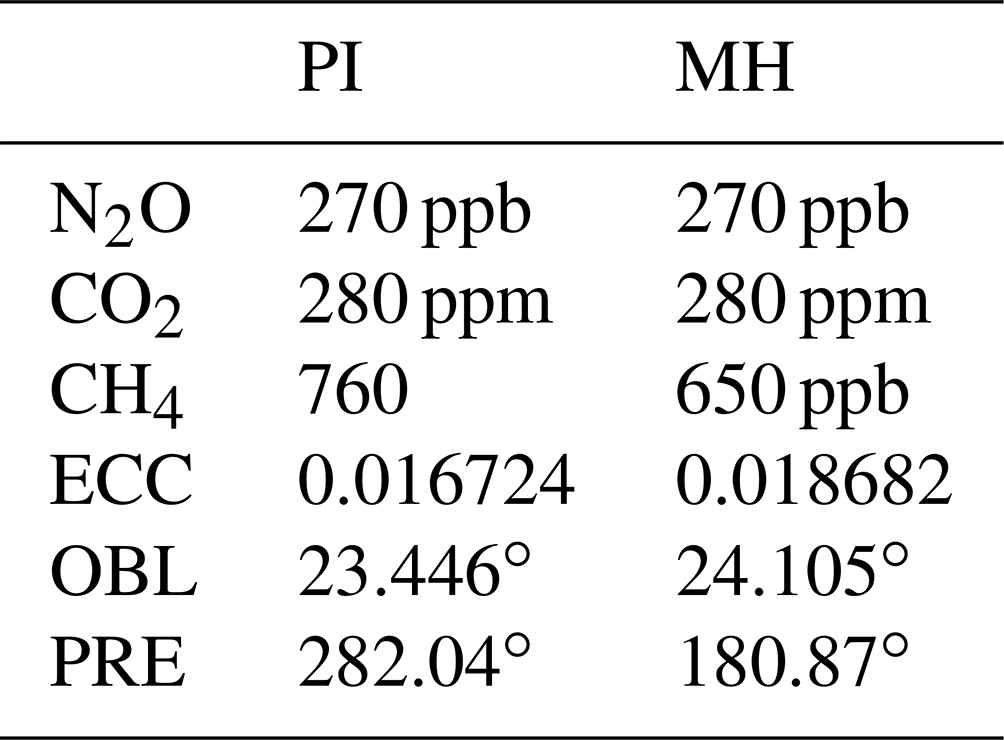
The model version used in this study is the COSMO-CLM 5.0_clm9. For its application to study past climates, the model needs to be modified to take into account changes in the Earth's configuration around the Sun on millennial timescales (i.e., changes in the eccentricity of the orbit, obliquity and precession). For this purpose a FORTRAN-based subroutine is implemented in the main radiation module of the model code, following the same approach of other paleoclimate studies (Russo and Cubasch, 2016; Prömmel et al., 2013; Fallah et al., 2016; Fallah et al., 2018). Additional changes to the model's code are required to account for different greenhouse gas concentrations in the past. An overview of the values of the orbital parameters and greenhouse gas concentrations used in the PI and the MH simulations (based on PMIP3 guidelines; see https://pmip3.lsce.ipsl.fr, last access: 1 June 2021) is presented in Table 1.
Table 1Values of orbital parameters and greenhouse gases concentrations for the PI (left) and MH (right) periods used for the conducted modeling experiments. The orbital parameters are the eccentricity of the orbit (ECC), the obliquity of the Earth's axis (OBL) and the precession of the equinoxes (PRE).
The entire model domain includes 125 grid points in the longitude and 122 grid points in latitude directions, with a spatial resolution of 0.44∘ (∼50 km), covering the whole of Europe. At each side of the domain, 10 grid points are used as a boundary relaxation zone and are excluded from the analysis. A map of the extension and topography of the inner domain of study is presented in Fig. 1.
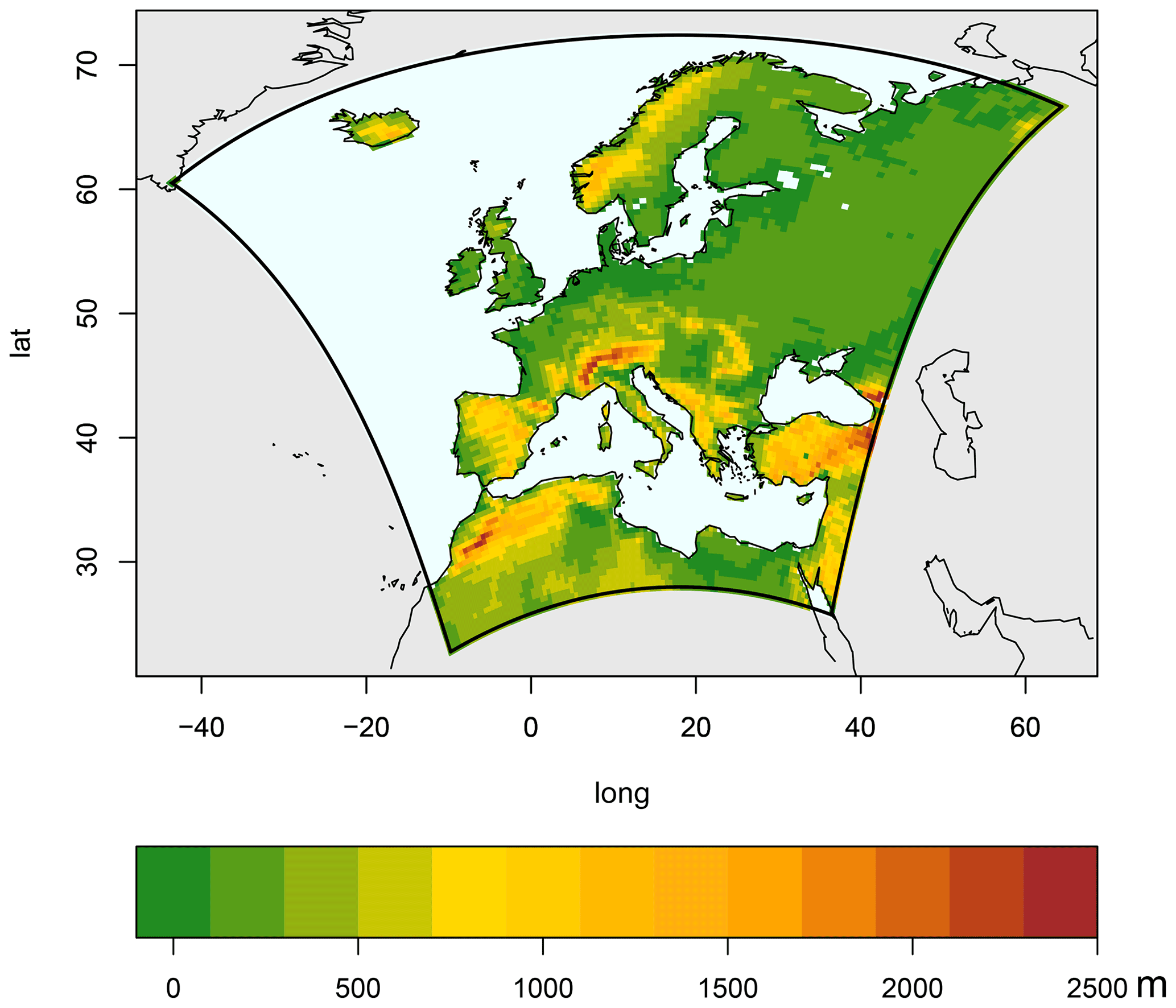
Figure 1Map of the topography and extension of the model domain.
All performed simulations are derived by applying changes to the setup of a reference run, using an “optimal” configuration slightly different than the most recent one proposed by the CLM-Community for Europe (Sørland et al., 2021). The reference run uses the Integrated Forecast System (IFS) model Tiedtke–Bechtold convection scheme (Bechtold et al., 2001) and a two-time-level Runge–Kutta scheme with time-split treatment of acoustic and gravity waves for time integration. It also uses a second-order Bott scheme for moisture variables and aerosol advection (Bott, 1989) and a prognostic turbulent kinetic energy (TKE) scheme for the vertical turbulent heat and momentum fluxes. Furthermore, a radiative transfer scheme (Ritter and Geleyn, 1992) and a one-moment, three-category (cloud ice, snow and graupel) ice scheme with prognostic treatment of the hydrometeors (Reinhardt and Seifert, 2006) are applied. The employed soil component is the multilayer soil model TERRA_LM (Schrodin and Heise, 2002; Schulz et al., 2016). TERRA_LM is a unidimensional soil–vegetation–atmosphere transfer scheme (SVAT) regulating momentum and heat fluxes between soil and the atmosphere. In TERRA_LM each grid point belongs to the same soil category throughout all soil depth. A total of eight soil types are available in the model: rock, ice, sand, sandy loam, loam, loamy clay, clay and peat. A set of parameters for each soil category is prescribed to the model, including the pore volume, heat capacity and hydraulic conductivity. A table with the different soil parameters and their values is provided in the Supplement. For the presented simulations, a map of soil categories derived from FAO (2003) is used.
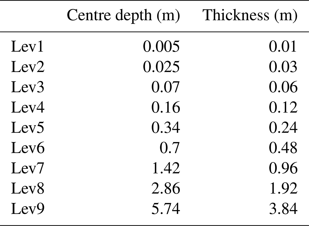
The reference run considers 50 atmospheric vertical layers, up to a height of 22 000 m, and a total of 9 hydrological active layers in the soil, down to a depth of 7.6 m. It also considers a treatment of the albedo based on dry and saturated soil. The main features of the reference simulation are summarized in Table 2, with information on the thickness and depth of the center of each of the different active soil layers reported in Table 3.
Table 2General description of model setup for the reference simulation.
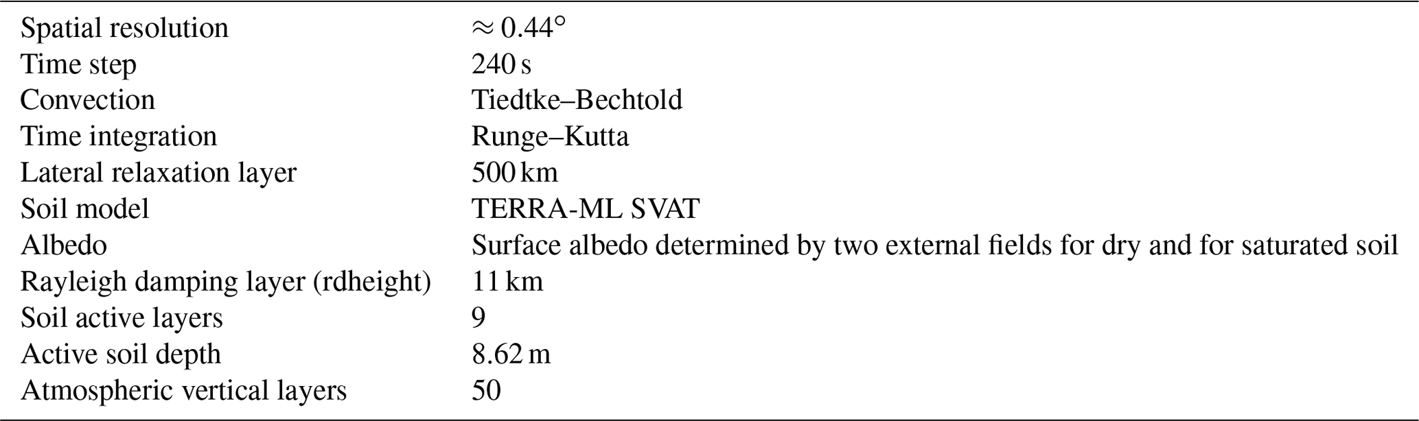
Table 3Depth of the center of the different active soil layers and their thickness in TERRA_LM.
Aiming to perform an extensive amount of sensitivity experiments in this study, targeting processes that could have an important impact at local and regional scales, the use of an RCM is mainly dictated by its relatively cheap computational demands. Even though the use of RCMs for paleoclimate applications has been disputed by a recent study by Armstrong et al. (2019), given that they are mainly limited by biases imposed at their lateral boundaries by the driving GCM, the fact that RCM outcomes vary significantly as a result of perturbations to their unconstrained parameter values and physical schemes (Bellprat et al., 2012a, b, 2016; Russo et al., 2019; Russo et al., 2020) supports its suitability for the purposes of this research.
2.2 Driving global circulation model
Initial and boundary data for the COSMO-CLM simulations are obtained from global simulations with the Max Planck Institute Earth system model in paleoclimate mode (MPI-ESM-P, Jungclaus et al., 2013). Output data with 6-hourly resolution are obtained from the MPI-ESM PI (Jungclaus et al., 2012a) and MH (Jungclaus et al., 2012b) simulations, respectively. The MPI-ESM includes coupled GCMs for the atmosphere and ocean as well as subsystem models for land and vegetation and for the marine biogeochemistry (Giorgetta et al., 2013). The atmospheric component ECHAM6 (Stevens et al., 2013) is run at T63 horizontal resolution (1.875∘ on a Gaussian grid) with 47 levels in the vertical. The ocean component used for the MPI-ESM-P simulations is the MPIOM (MPI Ocean Model, Jungclaus et al., 2006; Jungclaus et al., 2013). The ocean grid has a nominal resolution of 1.5∘ and considers 40 unevenly spaced levels in the vertical, ranging from 12 m near the surface to several hundred meters in the deep ocean (Jungclaus et al., 2013). The global simulations are conducted using the same values for the orbital parameters and GHG concentrations as the COSMO-CLM experiments in Table 1.
2.3 Physically perturbed ensemble
A total of 31 experiments for each of the considered periods (PI and MH) are performed to build a PPE, including the reference run, leading to a final set of 62 COSMO-CLM simulations. Starting from the reference configuration, selected parameters and physical options are perturbed consistently over the two periods. Most of the perturbed parameters are the ones for which the model has proven to be most sensitive for Europe (Bellprat et al., 2012a, 2016; Russo et al., 2020) and include at least one member for each of the main model schemes (i.e., turbulence, land-surface, convection, soil and radiation). A set of parameters is considered following the studies of Bellprat et al. (2012a, 2016). It affects sub-grid-scale cloud formation (uc1), shallow convection (entr_sc), interaction of radiation with clouds (radfac), turbulent transport of heat and moisture (tkhmin), exchange of heat and moisture between the atmosphere and the land surface (rlam_heat), strength of transpiration of the vegetation related to depth of rooting zone (facroot_dp2), and hydraulic cycling of soil moisture (soilhyd). Additionally, the parameters controlling heat exchange between the lower atmosphere and ocean (rat_sea), maximal turbulent length scale (tur_len), dissipation of turbulent heat and momentum (d_heat, d_mom), and the factor controlling the effective surface area (e_surf) are also considered, based on the sensitivity of the model as evinced from more recent studies (Russo et al., 2020).
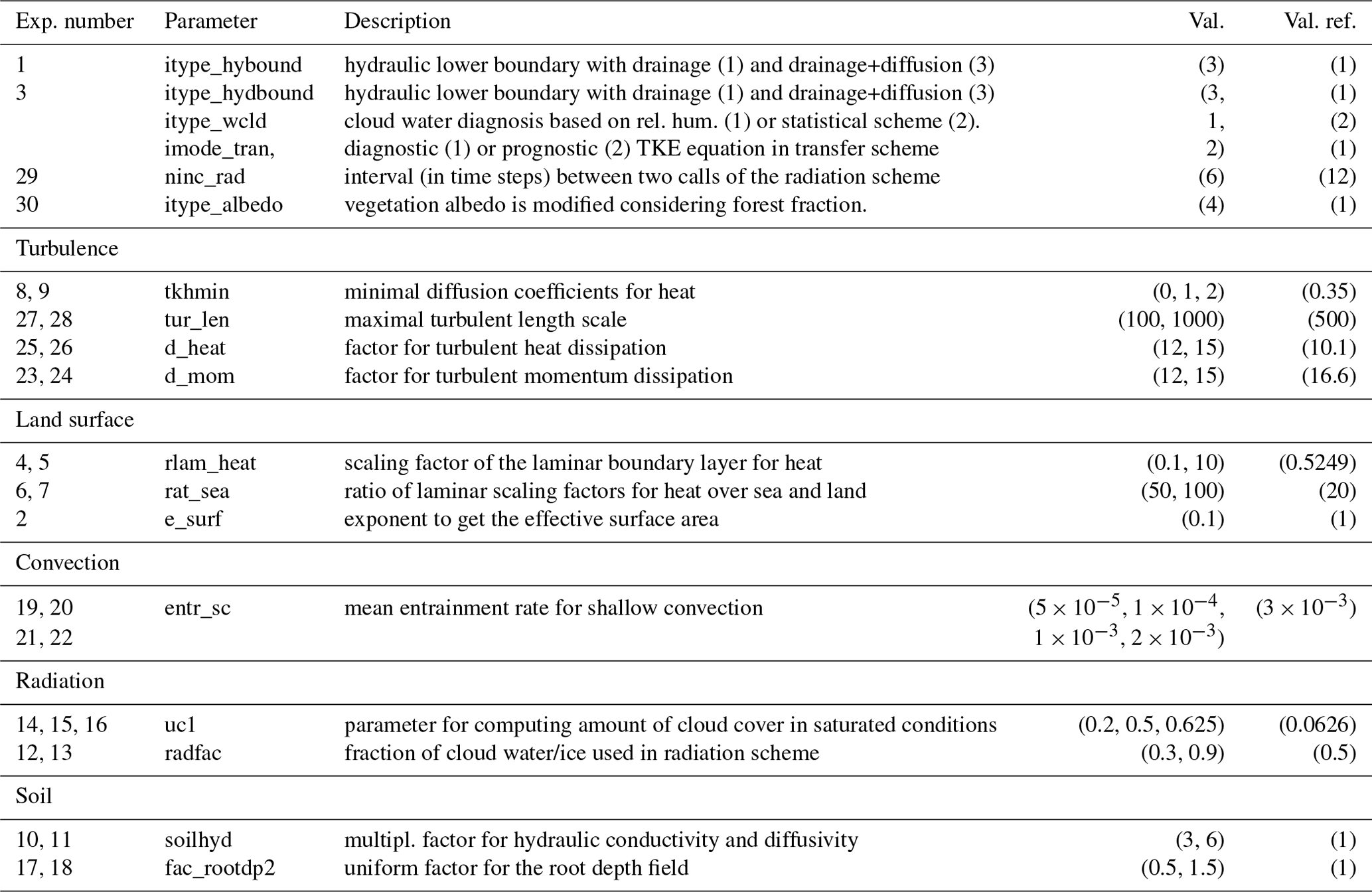
The explored physical options of the model are selected considering their potential to be sensitive to changes in radiative forcings, such as the interval of the call to the radiation scheme, the type of albedo representation and the soil hydraulic lower boundary with drainage and diffusion. A list of the different configurations tested starting from the one of the reference simulation is reported in Table 4, together with more detailed information. Each of these simulations covers 25 years, with 5 years considered as spin-up and excluded from the analysis. In total, the performed experiments with changes in the model configuration cover more than 1500 years of simulations. The set of conducted experiments is large enough to cover an extensive part of the parameter uncertainty of COSMO-CLM (Bellprat et al., 2012b, 2016), being the main target of objective calibration methods developed in recent years.
Table 4List of the 30 physical perturbed ensemble (PPE) experiments performed by perturbing the values of the corresponding parameters and physical options of the reference simulation. The values used in the considered experiments and the ones employed in the reference run are reported, respectively, in the last two columns of the table. The numbering does not include the reference run.
2.4 Perturbed initial soil moisture experiments
Eight additional simulations with perturbed soil moisture conditions are performed over a shorter period of 6 months. All these simulations are initialized on 1 April of the 15th year of the MH simulation period and use the same configuration as for the reference experiment of Sect. 2.3. The first of these experiments considers, for each point of the domain, each of the hydrological active soil layers as half-saturated at initialization. This means that a value of 50 % of relative soil moisture is set for each soil layer at the beginning of the simulation. The relative soil moisture is calculated considering the pore volume of each point of the domain, which is in COSMO-CLM a function of the soil type:
where Wso is the relative soil moisture for a given point with x and y coordinates i and j, respectively; Wl represents liquid water; Δz the depth of the considered soil layer z; and Vp is the pore volume of the given point (Baur et al., 2018).
Six additional simulations are then conducted, increasing and decreasing the initial relative soil moisture of the first run with half-saturated soil moisture, by 25 %, 50 % and 75 %, respectively. Another experiment is also conducted starting from fully saturated soil moisture conditions (+100 %) at initialization. Changes in the mean summer temperature of these experiments are analyzed with respect to the simulation with half-saturated initial soil moisture conditions.
For RCMs, the use of different boundaries (for example a different GCM or the same one with different forcing or configuration) could have a significant effect on the model results, often even more relevant than the employed RCM version or selected parameter values (Sørland et al., 2021). To take into account the effect of different boundaries on the sensitivity of the model to soil moisture perturbations, an additional set of 10 6-month long simulations are finally performed. More specifically, for each of five randomly selected years of the simulation period, two experiments with, respectively, an increase and a decrease of 75 % in soil moisture at the beginning of spring (with respect to half-saturated soil) are conducted.
As a matter of clarity, it is necessary to specify here that an increase (decrease) in soil moisture at initialization by, for example, +75 % (−75 %) corresponds to a total value of 87.5 % (12.5 %) of relative soil moisture.
2.5 Metrics for evaluating the assumption of stationarity of calibration approaches
The assumption of stationarity proper of calibration approaches is investigated here by means of the mean absolute error (MAE). Three variables that are normally used in RCM calibration procedures are considered (Bellprat et al., 2012a, b; Russo et al., 2020), namely near-surface temperature (T2M), precipitation (RR) and total cloud cover (CLCT).
In a first step, the MAE is calculated over daily mean anomalies for each of the three variables and each land point of the domain, for the PI and MH periods separately:
where e, V, i and j are the selected experiment, the considered variable, and the coordinates in the longitudinal and latitudinal directions of a given point, respectively. Additionally, d represents the considered day of the simulation period, with the total number of days D being 20×365. Finally, XN is the target simulation against which the bias is calculated (“nature” state). In a second step, the MAE is then calculated over regional monthly means, after subdividing the domain of study into a set of 10 sub-regions. The domain division is conducted similarly to regionalizations usually performed for Europe within the CORDEX framework or in other studies (Kotlarski et al., 2014; Bellprat et al., 2012a, b, 2016), assigning almost every point of the domain to a pre-defined climatic zone. A map of the 10 selected sub-regions is presented in Fig. 2. In this case the MAE is calculated as follows:
where, besides the same indices already introduced in Eq. (2), r indicates the considered sub-region (R=10) and m the given month ().
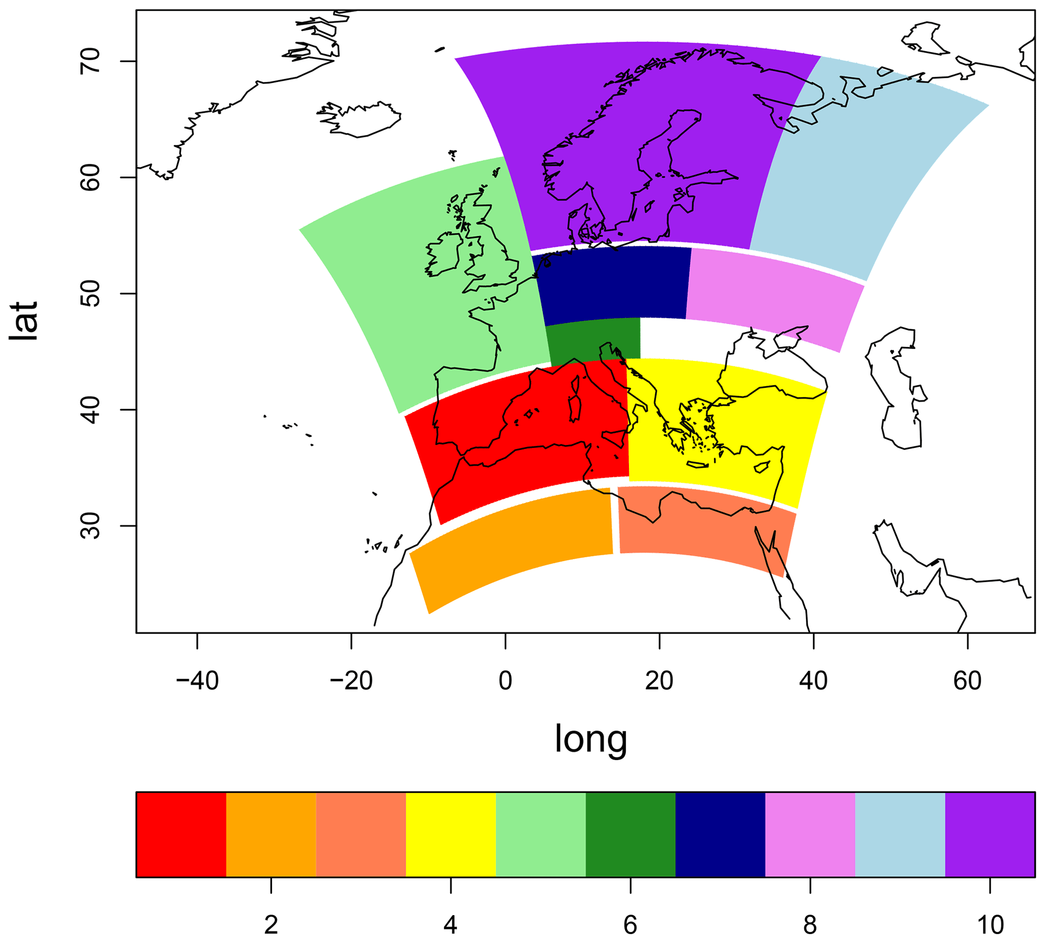
Figure 2Domain decomposition.
In both formulas for the calculation of the MAE (Eqs. 2 and 3), one of the model realizations is assumed as representative of the real state of the climate system in the two different periods. All the simulations are then ranked considering their distance from this “nature” realization. The reference simulation of Sect. 2.3 is considered in a first place as the “nature” state. Successively, for supporting the plausibility of the evinced results, the proposed analyses are reiterated using different realizations as the target for the calculation of the MAE.
3.1 PPE summer temperatures
In this section, PPE results are explored with the primary goal of discriminating processes that could possibly lead to a spatial pattern of summer mean near-surface temperatures at the MH closer to evidence from pollen-based reconstructions. For this purpose, the analyses focus on the anomalies between the MH and PI climatologies derived from the PPEs with different model configurations. Figure 3 shows the ensemble mean of the anomalies obtained by subtracting from the MH climatological mean of each realization the corresponding PI value. The mean anomalies are in a range of 0 to +2.5 ∘C. The mean model behavior does not show different results compared to other studies (Brewer et al., 2007; Mauri et al., 2014; Russo and Cubasch, 2016; Brierley et al., 2020), as the entire domain is characterized by a warming signal. This signal is heterogeneously distributed though, revealing a north-west to south-east gradient, with smaller anomalies over the British Isles, increasing towards eastern Europe and the Mediterranean region, and reaching a maximum in the area north of the Black Sea.
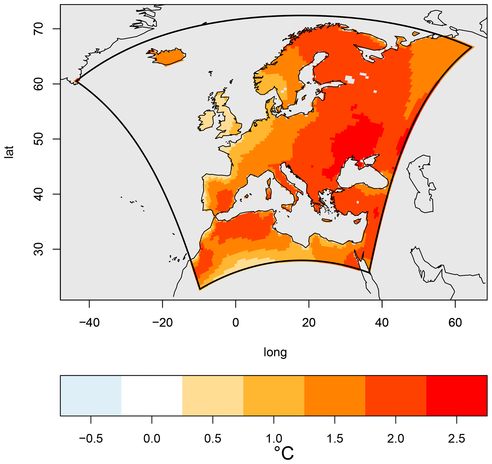
Figure 3Mean of the anomalies of summer (JJA) mean near-surface temperature calculated between each of the ensemble realizations, subtracting to the climatological value of the mid-Holocene (MH) the one obtained for the pre-industrial period (PI).
The maximum absolute differences in the MH–PI anomalies of summer temperatures, calculated for each point of the domain between the different ensemble members, are presented in Fig. 4. These differences are quite constrained, with values exceeding 0.5 ∘C only over parts of the Balkans and continental Europe. This is the result of a similar structural uncertainty of the model in summer for both periods (see the Supplement), indicating its limited ability in freely responding to changes in the forcing during the summer season, for any of the considered configurations. Basically, none of the tested model setups produces a remarkably different response, with respect to the other model states, for the two periods. This seems to be true not only for summer temperatures, but also for other seasons and variables (see the Supplement), pointing at a general stationarity of the model uncertainty under different forcing, at least when considering climatological values. In conclusion, none of the investigated changes in the model configuration, and associated processes, leads to summer temperatures over Europe that could be in better agreement with evidence from continental-scale pollen-based reconstructions.
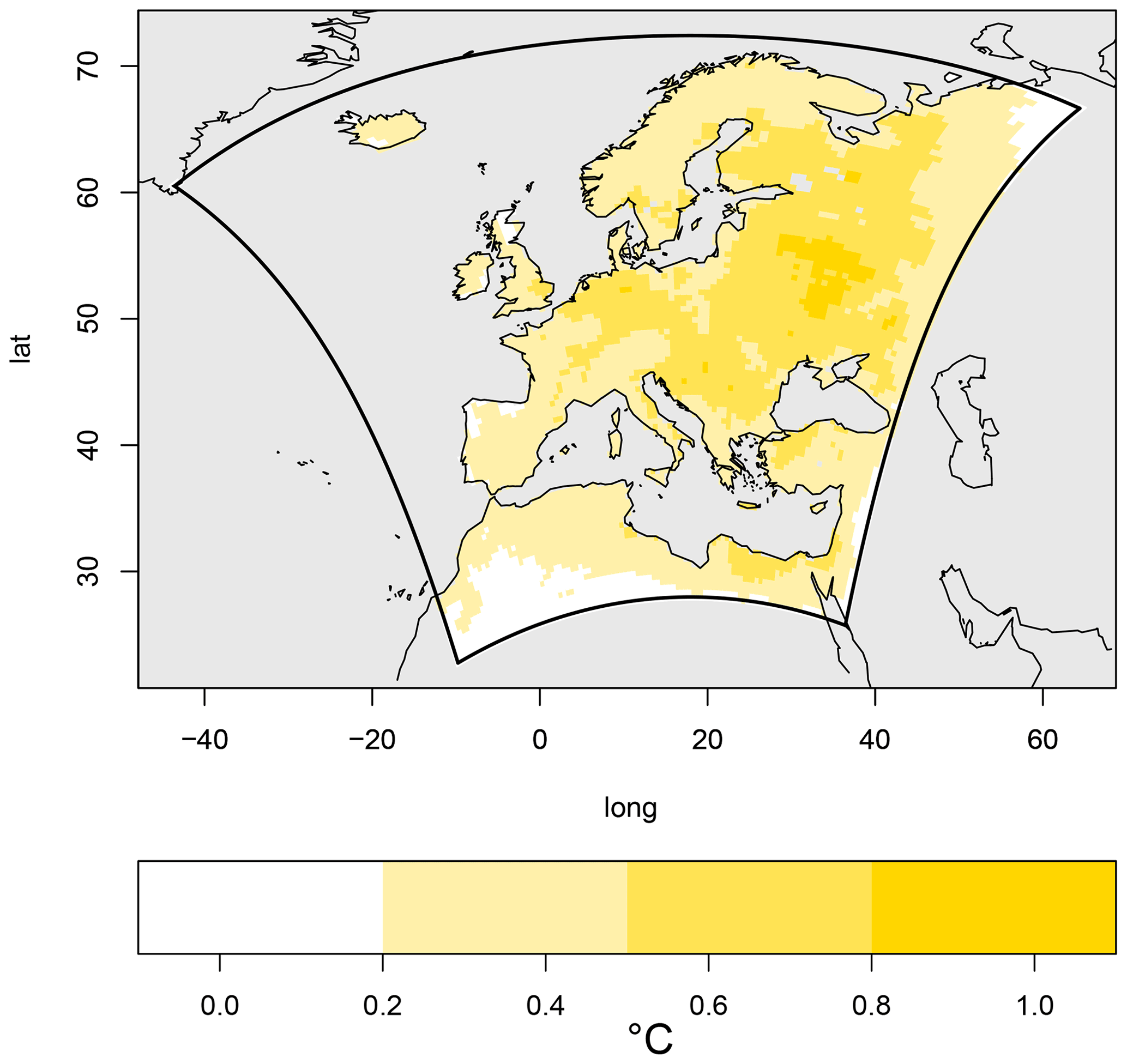
Figure 4Maximum absolute differences in MH–PI anomalies of summer (JJA) mean near-surface temperatures, calculated between the different ensemble members.
3.2 Perturbed soil moisture experiments
In this section, the results of the eight MH experiments with perturbed initial spring soil moisture conditions are presented. Figure 5 shows the differences in mean summer temperatures of the simulations with changes in initial spring soil moisture (25 %, 50 %, 75 % increase and decrease and 100 % increase) with respect to the simulation with half-saturated soil. Changes in available spring soil moisture seem to have an important effect on the simulated summer temperatures of the region (Fig. 5). In particular, there is a strong spatial dependency of the sensitivity of the model to moisture perturbation, with the areas of the Balkans and north of the Black Sea presenting the largest changes, up to 5 ∘C in the case of a reduction of initial soil moisture by 75 %. A similar spatial sensitivity is also evident for the model when considering different boundary conditions (see the Supplement).
Differences in summer temperatures are more pronounced for experiments with initially drier soil, generally presenting warmer conditions (Fig. 5, right column). In contrast, experiments with increased initial soil moisture lead to an overall cooling. In this case though, all the simulations present a very similar spatial distribution of summer temperatures (Fig. 5, left column), independently from the magnitude of the changes applied to the initial conditions. Analyzing the temporal evolution of soil moisture at the different model levels over the entire 6 months of simulation (Fig. 6), it is evident that the depletion of moisture is faster when more moisture is added to the initial conditions. This leads quickly to similar moisture availability at the beginning of summer in each of the considered cases, particularly in the upper soil levels. The experiments suggest that even if more soil moisture would be available in early spring in COSMO-CLM, as a consequence of, for example, increased late-winter precipitation, this would be depleted too quickly, leading to no appreciable changes in summer temperatures.
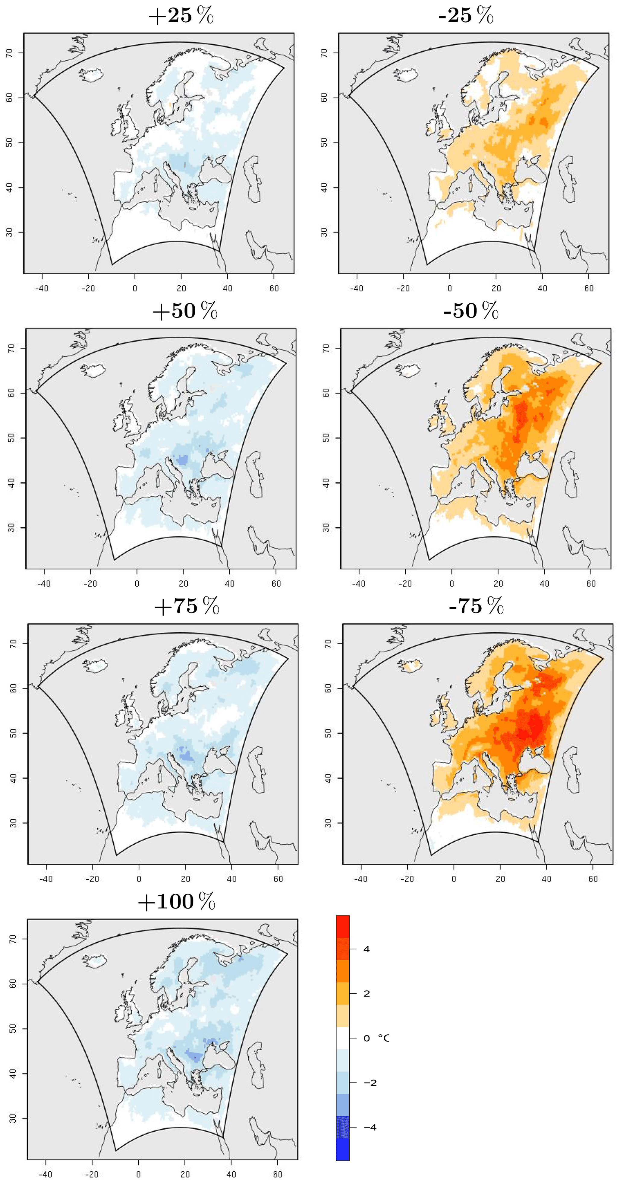
Figure 5Differences in summer (JJA) mean near-surface temperature calculated between each of the perturbed soil moisture experiments and the simulation with initial half-saturated soil levels. The left column shows the results of an increase in initial spring soil moisture by 25 %, 50 %, 75 % and 100 % from top to bottom, respectively. The right column shows the results obtained with drier initial soil moisture conditions, by 25 %, 50 % and 75 %.
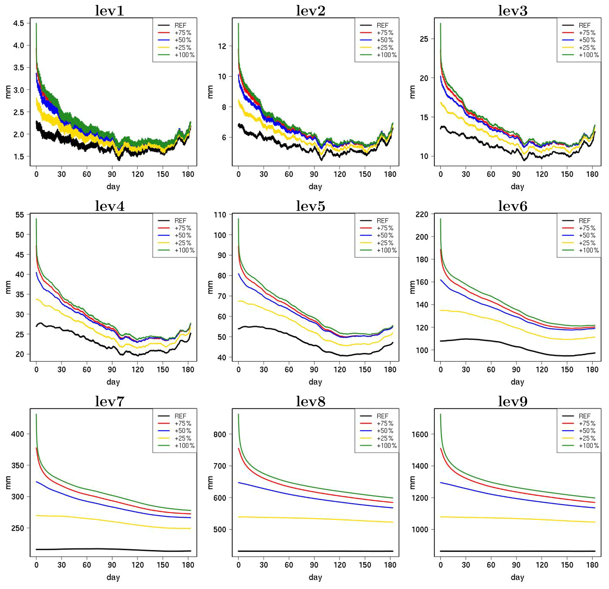
Figure 6Temporal evolution of soil moisture at the nine hydrological active layers (lev1 to lev9) for the experiments with increased initial soil moisture at the beginning of April. More detailed information on the depth and thickness of each layer can be found in Table 3. The data are shown from the first time step until the end of October of the same year of the simulations. The different experiments with added soil moisture and the reference run (REF: 50 % of relative soil moisture for all the points of the domain on 1 April) are indicated by different colors.
A similar model behavior is found for present-day studies, where a warm and dry bias of RCMs against observations over the Mediterranean region is attributed mainly to an overestimation of the evapotranspiration in spring, leading to an overly rapid depletion of soil moisture and, consequently, drier soil conditions in early summer (Seneviratne et al., 2010; Kotlarski et al., 2014; Davin et al., 2016). Davin et al. (2016) solved this issue by coupling the COSMO-CLM to a more complex soil scheme than the default TERRA_LM: the Community Land Model 4.0 (Oleson et al., 2010; Lawrence et al., 2011). In this way, they were able to sensibly reduce the warm summer bias of the model over the Mediterranean region and confirm the important role of land process representation to overcome this long-standing deficiency of climate models.
The experiments presented here cannot directly explain the disagreement between climate models and pollen-based reconstructions for MH summer temperatures over the Mediterranean region. However, they are particularly relevant since they confirm that pronounced regional differences in European summer temperatures during the MH may be related to soil–atmosphere interactions. In this context, the soil scheme of climate models applied to the study of European MH climate acquires significant importance. Considering the highlighted common model deficiencies related to soil–atmosphere coupling, known to notably affect simulated temperatures, a prerogative to any attempt to reconstruct the European climate at the MH using climate models is that the performances of their soil component must be first carefully evaluated, assessing its reliability in terms of retained spring soil moisture. The use of high-complexity soil schemes, as suggested for present-day studies, should be eventually considered.
Finally, it is also worth mentioning here that a present-day distribution of soil categories is used for the presented experiments. On millennial timescales, a possible source of uncertainty that needs to be additionally considered in modeling studies is the fact that soil might have changed with respect to the present day, for natural or anthropogenic reasons. This could have an impact on the moisture storage capacity of soil and, ultimately, on the simulated temperatures. This point should also be acknowledged in future studies of MH European climate using climate models.
3.3 Testing the assumption of stationarity of calibration approaches for RCMs
In this section, the PPEs produced for the PI and MH periods are used for testing whether an optimal model configuration for one period can also be assumed to be the best under different forcings. First, the analyses are conducted on daily mean anomalies calculated for each grid point of the domain and for each of the three considered variables separately.
The probability distribution functions (PDFs) of total cloud cover daily mean anomalies derived for each member of the ensemble, for a randomly selected point of sub-region 8, are depicted in Fig. 7 as an illustrative example. The PDF of the reference simulation for the PI period is highlighted in black and is considered as a theoretical “nature” state (what would typically be the target of a calibration). In the same figure (Fig. 7, left), the PDF of the PI experiment with the smallest MAE (Eq. 2) with respect to the “nature” state is represented by the red curve. All other ensemble realizations are plotted in light gray. For the MH (Fig. 7, right), the same colors are used for the same experiments. Thus, the red curve in the MH plot represents again the ensemble member closest to the reference run at the PI period. This aims to show how much the best simulation in one period (PI) diverges from the reference in the other (MH). In each panel of Fig. 7, the number of the best-performing experiment for the selected point, in terms of the MAE of Eq. (2), is reported in the top-left corner. The optimal realization changes in the two periods, with simulation 2 (with the exponent to get the effective surface area set to 0.1) being the best in one case, and experiment 26 (with the factor for turbulent heat dissipation set to 15) in the other.
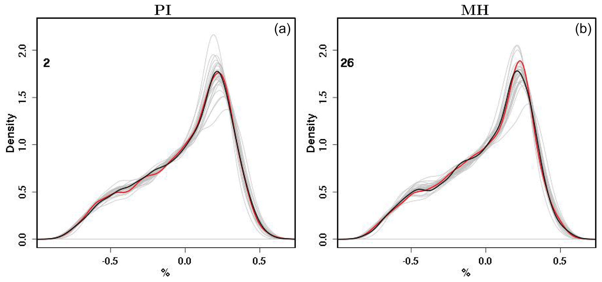
Figure 7Probability distribution functions of daily mean anomalies of total cloud cover calculated for the different ensemble realizations for the PI (a) and the MH (b) periods, for a randomly selected grid point in subregion 8 of Fig. 2. The PDF of the reference run, considered as the “nature” state, is highlighted in black. The realization with the minimum MAE with respect to the PI reference run is highlighted in red in both panels. Gray lines represent the remaining members of the ensembles for the two periods.
Considering the MAE calculated over the daily mean anomalies (Eq. 2) for each land point of the domain, the “best” model configuration changes in the two periods for over 91 % of the points for 2 m temperature, 92 % for precipitation and 89 % for total cloud cover. The same analyses assuming different realizations as the “nature” state, such as experiments 5 and 9, lead to similar conclusions.
These are further confirmed by additional analyses of the MAE calculated over monthly spatial means, usually being the target of calibration methods employed for COSMO-CLM. For all of the considered variables, no realization that performs best for one period maintains its “status” in the other (see the Supplement). The presented results are not dependent on the supposed “nature” state. Again, repeating the same analyses using a different realization as the target (as before, simulation 5 and simulation 9) leads in fact to similar conclusions.
These results suggest that using resources for the calibration of RCMs, in order to determine an optimal model configuration, might not be the most ideal approach for the study of future and past climate. The production of small PPEs sampling a good part of a model structural uncertainty and likely to contain the best model answer under different forcing would be a preferable option to follow instead.
In this study, the regional climate model COSMO-CLM is used with the main goal of gaining a better understanding of the possible drivers of the long-standing mismatch between outcomes of climate model simulations and pollen-based reconstructions of mid-Holocene (MH) summer temperatures over Europe. Additionally, trying to learn from the past for the future, the study also uses the MH climate as a test-bed for investigating appropriate approaches for the performance of reliable climate simulations.
Two physically perturbed ensembles (PPEs) are produced to assess how the model reacts, for different parameter values and physical options, to changes in the radiative forcing over two distinct time spans (pre-industrial, PI, and MH). The mean differences in seasonal summer temperatures calculated between realizations with the same model configuration for the two considered periods show generally warmer conditions at the MH over all of Europe, consistently with the results of previous modeling studies. In general, each member of the produced PPE does not behave remarkably different with respect to the other ensemble members for both the MH and PI periods. The maximum differences in the anomalies of summer temperatures between the two periods, calculated among the different ensemble members, are in fact very much constrained over most of the domain of study. This indicates a limited sensitivity of the model to changes in the climate forcing in terms of its structural uncertainty, suggesting that none of the investigated changes in model configuration, and the associated physical processes, leads to remarkable variations in European summer temperatures closer to the evidence of continental-scale pollen-based reconstructions.
Furthermore, additional sensitivity tests are conducted for the mid-Holocene by perturbing the model initial soil moisture conditions at the beginning of spring. These experiments show that, for COSMO-CLM, there is a strong spatial dependency of European summer near-surface temperatures on the soil moisture available in spring. Remarkable differences are particularly evident over the Balkans and the area north of the Black Sea, with an increase of up to 5 ∘C when decreasing the initial soil moisture values by 75 %. The differences are more pronounced for the simulations with drier initial conditions, compared to the ones with enhanced soil moisture. For the latter, similar spatial patterns of colder summer temperatures are evident for all of the considered initial perturbations. Analyses of the temporal evolution of soil moisture show that adding moisture to the initial conditions leads to a faster depletion, confirming a deficiency of the considered land scheme of COSMO-CLM in properly retaining spring soil moisture, already known from present-day studies. Such deficiency, known to be one of the main reasons for a common warm bias of climate models in European summer temperatures, has never been carefully taken into account in modeling studies of the MH climate. The presented results emphasize the role of soil–atmosphere interactions as one of the possible drivers of the differences in European pollen-based summer temperatures at the MH. At the same time, they highlight the importance of properly evaluating the skills of the soil component of a given climate model in retaining spring soil moisture when investigating MH European climate. The consideration of more sophisticated soil schemes may be necessary to bridge the gap between models and proxy reconstructions, possibly contributing to the solution of this long-standing dilemma.
Finally, the analysis of the distribution of the PPEs for different variables (T2, PREC, TCLC) shows that, in almost all of the considered cases, an optimal model configuration in one period does not seem to be the best in another characterized by different radiative forcing. The ranking (based on the mean absolute error) of the single realizations changes each time. These results raise concerns about the usefulness of automatic and objective calibration methods for RCMs. Since there is no guarantee that an optimal model configuration maintains its status over different periods of time, it might make sense to better channel computational resources. An effective use of resources is of fundamental importance for the production of climate projections and should be considered as one of the main priorities of future climate studies. The presented results suggest that a better approach to the calibration of RCMs is the production of small PPEs that target a set of model configurations, properly representing climate phenomena characteristic of the target region and that will be likely to contain the best model answer under different forcing.
Simulation configuration files can be downloaded from https://doi.org/10.5281/zenodo.5140094 (Russo, 2021b).
All the data for the mid-Holocene period with which the presented analyses are conducted are available at the following link: https://doi.org/10.5281/zenodo.5138131 (Russo, 2021c).
All the data for the pre-industrial period with which the presented analyses are conducted are available at the following link: https://doi.org/10.5281/zenodo.5140034 (Russo, 2021d).
Additional data used for the performance of the presented simulations, such as land/surface parameters, as well as the interpolated boundaries with soil moisture conditions at 50 % saturation, are available at the following link: https://doi.org/10.5281/zenodo.5140079 (Russo, 2021a).
The R scripts used for conducting the presented analyses are available at https://doi.org/10.5281/zenodo.5144973 (Russo, 2021e).
A complete documentation of the COSMO-Model is permanently available at the following link: https://www.dwd.de/EN/ourservices/cosmo_documentation/cosmo_documentation.html (last access: 1 June 2021).
The COSMO-CLM model is completely free of charge for all research applications. The version of the COSMO-CLM model used in this study can be downloaded from the following website: https://redc.clm-community.eu/projects/cclm-sp/wiki/Downloads (last access: 1 June 2021). Access is license-restricted (http://www.cosmo-model.org/content/consortium/licencing.htm, last access: 1 June 2021), and for the download the user needs to become a member of the CLM-Community, or the respective institute needs to hold an institutional license.
The supplement related to this article is available online at: https://doi.org/10.5194/cp-18-895-2022-supplement.
ER designed the study and performed the simulations. ER, BF, PL, MK and CCR equally contributed to the interpretation of the results, the drafting of the manuscript and to scientific discussion.
The contact author has declared that neither they nor their co-authors have any competing interests.
Publisher’s note: Copernicus Publications remains neutral with regard to jurisdictional claims in published maps and institutional affiliations.
Christoph C. Raible is supported by the Swiss National Science Foundation (SNF) within the project “PleistoCEP”. Patrick Ludwig is supported by the Helmholtz Climate Initiative REKLIM (regional climate change; https://www.reklim.de/en, last access: 1 February 2022). Bijan Fallah is supported by the German Federal Foreign Office through the Green Central Asia project (http://greencentralasia.org/en, last access: 1 February 2022). Data are locally stored on the oschgerstore provided by the Oeschger Center for Climate Change Research (OCCR).
The computational resources necessary for conducting the experiments presented in this research were made available by the German Climate Computing Center (DKRZ). The authors are also particularly grateful to the COSMO and the CLM-Community for all their efforts in developing the COSMO-CLM model and making its code available.
Finally, a special thanks goes to the editor and the two anonymous reviewers for their constructive comments, which helped to sensibly improve the paper.
This research has been supported by the Swiss National Science Foundation (SNF) within the project “PleistoCEP” (grant no. 200020_172745), the Helmholtz Climate Initiative REKLIM, and the German Federal Foreign Office through the Green Central Asia project.
This paper was edited by Hugues Goosse and reviewed by two anonymous referees.
Armstrong, E., Hopcroft, P., and Valdes, P.: Reassessing the value of regional climate modeling using paleoclimate simulations, Geophys. Res. Lett., 46, 12464–12475, 2019. a
Baldauf, M., Seifert, A., Förstner, J., Majewski, D., Raschendorfer, M., and Reinhardt, T.: Operational convective-scale numerical weather prediction with the COSMO model: Description and sensitivities, Mon. Weather Rev., 139, 3887–3905, 2011. a
Bartlein, P., Harrison, S., and Izumi, K.: Underlying causes of Eurasian midcontinental aridity in simulations of mid-Holocene climate, Geophys. Res. Lett., 44, 9020–9028, 2017. a
Baur, F., Keil, C., and Craig, G.: Soil moisture–precipitation coupling over Central Europe: Interactions between surface anomalies at different scales and the dynamical implication, Q. J. Roy. Meteor. Soc., 144, 2863–2875, 2018. a
Bechtold, P., Bazile, E., Guichard, F., Mascart, P., and Richard, E.: A mass-flux convection scheme for regional and global models, Q. J. Roy. Meteor. Soc., 127, 869–886, 2001. a
Bellprat, O., Kotlarski, S., Lüthi, D., and Schär, C.: Objective calibration of regional climate models, J. Geophys. Res., 117, D23115, https://doi.org/10.1029/2012JD018262, 2012a. a, b, c, d, e, f, g, h, i
Bellprat, O., Kotlarski, S., Lüthi, D., and Schär, C.: Exploring perturbed physics ensembles in a regional climate model, J. Climate, 25, 4582–4599, 2012b. a, b, c, d, e
Bellprat, O., Kotlarski, S., Lüthi, D., De Elía, R., Frigon, A., Laprise, R., and Schär, C.: Objective calibration of regional climate models: application over Europe and North America, J. Climate, 29, 819–838, 2016. a, b, c, d, e, f, g
Berger, A.: Long-term variations of daily insolation and Quaternary climatic changes, J. Atmos. Sci., 35, 2362–2367, 1978. a
Berger, A.: Milankovitch and climate: understanding the response to astronomical forcing, vol. 126, Springer Science & Business Media, https://doi.org/10.1007/978-94-017-4841-4, 2013. a
Berger, A. and Loutre, M.-F.: Insolation values for the climate of the last 10 million years, Quaternary Sci. Rev., 10, 297–317, 1991. a
Boberg, F. and Christensen, J.: Overestimation of Mediterranean summer temperature projections due to model deficiencies, Nat. Clim. Change, 2, 433–436, 2012. a
Bonfils, C., de Noblet-Ducoudré, N., Guiot, J., and Bartlein, P.: Some mechanisms of mid-Holocene climate change in Europe, inferred from comparing PMIP models to data, Clim. Dynam., 23, 79–98, 2004. a
Bott, A.: A positive definite advection scheme obtained by nonlinear renormalization of the advective fluxes, Mon. Weather Rev., 117, 1006–1016, 1989. a
Brewer, S., Guiot, J., and Torre, F.: Mid-Holocene climate change in Europe: a data-model comparison, Clim. Past, 3, 499–512, https://doi.org/10.5194/cp-3-499-2007, 2007. a, b
Brierley, C. M., Zhao, A., Harrison, S. P., Braconnot, P., Williams, C. J. R., Thornalley, D. J. R., Shi, X., Peterschmitt, J.-Y., Ohgaito, R., Kaufman, D. S., Kageyama, M., Hargreaves, J. C., Erb, M. P., Emile-Geay, J., D'Agostino, R., Chandan, D., Carré, M., Bartlein, P. J., Zheng, W., Zhang, Z., Zhang, Q., Yang, H., Volodin, E. M., Tomas, R. A., Routson, C., Peltier, W. R., Otto-Bliesner, B., Morozova, P. A., McKay, N. P., Lohmann, G., Legrande, A. N., Guo, C., Cao, J., Brady, E., Annan, J. D., and Abe-Ouchi, A.: Large-scale features and evaluation of the PMIP4-CMIP6 midHolocene simulations, Clim. Past, 16, 1847–1872, https://doi.org/10.5194/cp-16-1847-2020, 2020. a, b
Carvalho, D., Cardoso Pereira, S., and Rocha, A.: Future surface temperatures over Europe according to CMIP6 climate projections: an analysis with original and bias-corrected data, Climatic Change, 167, 1–17, 2021. a
Cattiaux, J., Douville, H., and Peings, Y.: European temperatures in CMIP5: origins of present-day biases and future uncertainties, Clim. Dynam., 41, 2889–2907, 2013. a
Cheddadi, R., Yu, G., Guiot, J., Harrison, S., and Prentice, I.: The climate of Europe 6000 years ago, Clim. Dynam., 13, 1–9, 1996. a, b
Christensen, J. H., Boberg, F., Christensen, O. B., and Lucas-Picher, P.: On the need for bias correction of regional climate change projections of temperature and precipitation, Geophys. Res. Lett., 35, L20709, https://doi.org/10.1029/2008GL035694, 2008. a
Davin, E., Maisonnave, E., and Seneviratne, S.: Is land surface processes representation a possible weak link in current Regional Climate Models?, Environ. Res. Lett., 11, 074027, https://doi.org/10.1088/1748-9326/11/7/074027, 2016. a, b, c
Davis, B., Brewer, S., Stevenson, A., and Guiot, J.: The temperature of Europe during the Holocene reconstructed from pollen data, Quaternary Sci. Rev., 22, 1701–1716, 2003. a, b
Fallah, B., Sodoudi, S., and Cubasch, U.: Westerly jet stream and past millennium climate change in Arid Central Asia simulated by COSMO-CLM model, Theor. Appl. Climatol., 124, 1079–1088, 2016. a
Fallah, B., Russo, E., Acevedo, W., Mauri, A., Becker, N., and Cubasch, U.: Towards high-resolution climate reconstruction using an off-line data assimilation and COSMO-CLM 5.00 model, Clim. Past, 14, 1345–1360, https://doi.org/10.5194/cp-14-1345-2018, 2018. a
Fischer, N. and Jungclaus, J. H.: Evolution of the seasonal temperature cycle in a transient Holocene simulation: orbital forcing and sea-ice, Clim. Past, 7, 1139–1148, https://doi.org/10.5194/cp-7-1139-2011, 2011. a
FAO (Food and Agriculture Organization of the United Nations): Digital soil map of the world and derived soil properties, FAO, Land and Water Development Division, ISBN 9789251048955, 2003. a
Forest, C., Stone, P., Sokolov, A., Allen, M., and Webster, M.: Quantifying uncertainties in climate system properties with the use of recent climate observations, Science, 295, 113–117, 2002. a
Giorgetta, M. A., Jungclaus, J., Reick, C. H., Legutke, S., Bader, J., Böttinger, M., Brovkin, V., Crueger, T., Esch, M., Fieg, K., Glushak, K., Gayler, V., Haak, H., Hollweg, H.-D., Ilyina, T., Kinne, S., Kornblueh, L., Matei, D., Mauritsen, T., Mikolajewicz, U., Mueller, W., Notz, D., Pithan, F., Raddatz, T., Rast, S., Redler, R., Roeckner, E., Schmidt, H., Schnur, R., Segschneider, J., Six, K. D., Stockhause, M., Timmreck, C., Wegner, J., Widmann, H., Wieners, K.-H., Claussen, M., Marotzke, J., and Stevens, B.: Climate and carbon cycle changes from 1850 to 2100 in MPI-ESM simulations for the Coupled Model Intercomparison Project phase 5, J. Adv. Model. Earth Sy., 5, 572–597, https://doi.org/10.1002/jame.20038, 2013. a
Hauser, T., Keats, A., and Tarasov, L.: Artificial neural network assisted Bayesian calibration of climate models, Clim. Dynam., 39, 137–154, 2012. a
Haywood, A., Valdes, P., Aze, T., Barlow, N., Burke, A., Dolan, A., Von Der Heydt, A., Hill, D., Jamieson, S., Otto-Bliesner, B., Salzmann, U., Saupe, E., and Voss, J.: What can Palaeoclimate Modelling do for you?, Earth Systems and Environment, 3, 1–18, 2019. a
Hourdin, F., Mauritsen, T., Gettelman, A., Golaz, J.-C., Balaji, V., Duan, Q., Folini, D., Ji, D., Klocke, D., Qian, Y., Rauser, F., Rio, C., Tomassini, L., Watanabe, M., and Williamson, D.: The art and science of climate model tuning, B. Am. Meteorol. Soc., 98, 589–602, 2017. a
Huntley, B. and Prentice, I.: July temperatures in Europe from pollen data, 6000 years before present, Science, 241, 687–690, 1988. a, b
Jungclaus, J., Keenlyside, N., Botzet, M., Haak, H., Luo, J., Latif, M., Marotzke, J., Mikolajewicz, U., and Roeckner, E.: Ocean circulation and tropical variability in the coupled model ECHAM5/MPI-OM, J. Climate, 19, 3952–3972, 2006. a
Jungclaus, J., Giorgetta, M., Reick, C., Legutke, S., Brovkin, V., Crueger, T., Esch, M., Fieg, K., Fischer, N., Glushak, K., Gayler, V., Haak, H., Hollweg, H., Kinne, S., Kornblueh, L., Matei, D., Mauritsen, T., Mikolajewicz, U., Müller, W., Notz, D., Pohlmann, T., Raddatz, T., Rast, S., Roeckner, E., Salzmann, M., Schmidt, H., Schnur, R., Segschneider, J., Six, K., Stockhause, M., Wegner, J., Widmann, H., Wieners, K., Claussen, M., Marotzke, J., and Stevens, B.: CMIP5 simulations of the Max Planck Institute for Meteorology (MPI-M) based on the MPI-ESM-P model: The piControl experiment, served by ESGF, WDCC [data set], https://doi.org/10.1594/WDCC/CMIP5.MXEPpc, 2012a. a
Jungclaus, J., Giorgetta, M., Reick, C., Legutke, S., Brovkin, V., Crueger, T., Esch, M., Fieg, K., Fischer, N., Glushak, K., Gayler, V., Haak, H., Hollweg, H., Kinne, S., Kornblueh, L., Matei, D., Mauritsen, T., Mikolajewicz, U., Müller, W., Notz, D., Pohlmann, T., Raddatz, T., Rast, S., Roeckner, E., Salzmann, M., Schmidt, H., Schnur, R., Segschneider, J., Six, K., Stockhause, M., Wegner, J., Widmann, H., Wieners, K., Claussen, M., Marotzke, J., and Stevens, B.: CMIP5 simulations of the Max Planck Institute for Meteorology (MPI-M) based on the MPI-ESM-P model: The midHolocene experiment, served by ESGF, WDCC [data set], https://doi.org/10.1594/WDCC/CMIP5.MXEPmh, 2012b. a
Jungclaus, J. H., Fischer, N., Haak, H., Lohmann, K., Marotzke, J., Matei, D., Mikolajewicz, U., Notz, D., and von Storch, J. S.: Characteristics of the ocean simulations in the Max Planck Institute Ocean Model (MPIOM) the ocean component of the MPI-Earth system model, J. Adv. Model. Earth Sy., 5, 422–446, https://doi.org/10.1002/jame.20023, 2013. a, b, c
Knutti, R., Stocker, T., Joos, F., and Plattner, G.: Constraints on radiative forcing and future climate change from observations and climate model ensembles, Nature, 416, 719–723, 2002. a
Kotlarski, S., Keuler, K., Christensen, O. B., Colette, A., Déqué, M., Gobiet, A., Goergen, K., Jacob, D., Lüthi, D., van Meijgaard, E., Nikulin, G., Schär, C., Teichmann, C., Vautard, R., Warrach-Sagi, K., and Wulfmeyer, V.: Regional climate modeling on European scales: a joint standard evaluation of the EURO-CORDEX RCM ensemble, Geosci. Model Dev., 7, 1297–1333, https://doi.org/10.5194/gmd-7-1297-2014, 2014. a, b, c
Lawrence, D., Oleson, K., Flanner, M., Thornton, P., Swenson, S., Lawrence, P., Zeng, X., Yang, Z., Levis, S., Sakaguchi, K., Bonan, B., and Slater, A.: Parameterization improvements and functional and structural advances in version 4 of the Community Land Model, J. Adv. Model. Earth Sy., 3, M03001, https://doi.org/10.1029/2011MS00045, 2011. a
Loutre, M. F., Mouchet, A., Fichefet, T., Goosse, H., Goelzer, H., and Huybrechts, P.: Evaluating climate model performance with various parameter sets using observations over the recent past, Clim. Past, 7, 511–526, https://doi.org/10.5194/cp-7-511-2011, 2011. a
Masson, V., Cheddadi, R., Braconnot, P., Joussaume, S., Texier, D., and PMIP participants: Mid-Holocene climate in Europe: what can we infer from PMIP model-data comparisons?, Clim. Dynam., 15, 163–182, 1999. a, b
Mauri, A., Davis, B. A. S., Collins, P. M., and Kaplan, J. O.: The influence of atmospheric circulation on the mid-Holocene climate of Europe: a data–model comparison, Clim. Past, 10, 1925–1938, https://doi.org/10.5194/cp-10-1925-2014, 2014. a, b, c
Mauri, A., Davis, B., Collins, P., and Kaplan, J.: The climate of Europe during the Holocene: a gridded pollen-based reconstruction and its multi-proxy evaluation, Quaternary Sci. Rev., 112, 109–127, 2015. a, b, c, d
Mauritsen, T., Stevens, B., Roeckner, E., Crueger, T., Esch, M., Giorgetta, M., Haak, H., Jungclaus, J., Klocke, D., Matei, D., Mikolajewicz, U., Notz, D., Pincus, R., Schmidt, H., and Tomassin, L.: Tuning the climate of a global model, J. Adv. Model. Earth Sy., 4, M00A01, https://doi.org/10.1029/2012MS000154, 2012. a
Murphy, J., Sexton, D., Barnett, D., Jones, G., Webb, M., Collins, M., and Stainforth, D.: Quantification of modelling uncertainties in a large ensemble of climate change simulations, Nature, 430, 768–772, 2004. a
Oleson, K., Lawrence, D., Gordon, B., Flanner, M., Kluzek, E., Peter, J., Levis, S., Swenson, S., Thornton, E., Feddema, J., Heald, C., Lamarque, J., Niu, G., Qian, T., Running, S., Sakaguchi, K., Yang, L., Zeng, X., Zeng, X., and Decker, M.: Technical description of version 4.0 of the Community Land Model (CLM), No. NCAR/TN-478+STR, University Corporation for Atmospheric Research, https://doi.org/10.5065/D6FB50WZ, 2010. a
Otto-Bliesner, B. L., Braconnot, P., Harrison, S. P., Lunt, D. J., Abe-Ouchi, A., Albani, S., Bartlein, P. J., Capron, E., Carlson, A. E., Dutton, A., Fischer, H., Goelzer, H., Govin, A., Haywood, A., Joos, F., LeGrande, A. N., Lipscomb, W. H., Lohmann, G., Mahowald, N., Nehrbass-Ahles, C., Pausata, F. S. R., Peterschmitt, J.-Y., Phipps, S. J., Renssen, H., and Zhang, Q.: The PMIP4 contribution to CMIP6 – Part 2: Two interglacials, scientific objective and experimental design for Holocene and Last Interglacial simulations, Geosci. Model Dev., 10, 3979–4003, https://doi.org/10.5194/gmd-10-3979-2017, 2017. a
Prömmel, K., Cubasch, U., and Kaspar, F.: A regional climate model study of the impact of tectonic and orbital forcing on African precipitation and vegetation, Palaeogeogr. Palaeocl., 369, 154–162, 2013. a
Reinhardt, T. and Seifert, A.: A three-category ice scheme for LMK, Cosmo Newsletter, 6, 115–120, 2006. a
Ritter, B. and Geleyn, J.: A comprehensive radiation scheme for numerical weather prediction models with potential applications in climate simulations, Mon. Weather Rev., 120, 303–325, 1992. a
Rockel, B., Will, A., and Hense, A.: The regional climate model COSMO-CLM (CCLM), Meteorol. Z., 17, 347–348, 2008. a, b
Russo, E.: Additional data simulations COSMO-CLM Russo et al. 2021, Climate of the Past, Version 1, Zenodo [data set], https://doi.org/10.5281/zenodo.5140079, 2021a. a
Russo, E.: Collection of Namelist of PI simulations with COSMO-CLM (Russo et al. 2021, Climate of the Past), Version 1, Zenodo [data set], https://doi.org/10.5281/zenodo.5140094, 2021b. a
Russo, E.: Data MH simulations COSMO-CLM Russo et al. 2021, Climate of the Past, Version 1, Zenodo [data set], https://doi.org/10.5281/zenodo.5138131, 2021c. a
Russo, E.: Data PI simulations COSMO-CLM Russo et al. 2021, Climate of the Past, Version 1, Zenodo [data set], https://doi.org/10.5281/zenodo.5140034, 2021d. a
Russo, E.: Scripts Analysis Russo et al. 2021, Climate of the Past, Version 1, Zenodo [data set], https://doi.org/10.5281/zenodo.5144973, 2021e. a
Russo, E. and Cubasch, U.: Mid-to-late Holocene temperature evolution and atmospheric dynamics over Europe in regional model simulations, Clim. Past, 12, 1645–1662, https://doi.org/10.5194/cp-12-1645-2016, 2016. a, b, c, d, e, f
Russo, E., Kirchner, I., Pfahl, S., Schaap, M., and Cubasch, U.: Sensitivity studies with the regional climate model COSMO-CLM 5.0 over the CORDEX Central Asia Domain, Geosci. Model Dev., 12, 5229–5249, https://doi.org/10.5194/gmd-12-5229-2019, 2019. a, b
Russo, E., Sørland, S. L., Kirchner, I., Schaap, M., Raible, C. C., and Cubasch, U.: Exploring the parameter space of the COSMO-CLM v5.0 regional climate model for the Central Asia CORDEX domain, Geosci. Model Dev., 13, 5779–5797, https://doi.org/10.5194/gmd-13-5779-2020, 2020. a, b, c, d, e
Samartin, S., Heiri, O., Joos, F., Renssen, H., Franke, J., Brönnimann, S., and Tinner, W.: Warm Mediterranean mid-Holocene summers inferred from fossil midge assemblages, Nat. Geosci., 10, 207–212, 2017. a, b
Schrodin, R. and Heise, E.: The Multi-Layer Version of the DWD Soil Model TERRA-LM, COSMO Tech. Rep., no. 2, http://www.cosmo-model.org/content/model/documentation/techReports/docs/techReport02.pdf (last access: 1 June 2021), 2002. a
Schulz, J., Vogel, G., Becker, C., Kothe, S., Rummel, U., and Ahrens, B.: Evaluation of the ground heat flux simulated by a multi-layer land surface scheme using high-quality observations at grass land and bare soil, Meteorol. Z., 25, 607–620, https://doi.org/10.1127/metz/2016/0537, 2016. a
Seneviratne, S., Lüthi, D., Litschi, M., and Schär, C.: Land–atmosphere coupling and climate change in Europe, Nature, 443, 205–209, 2006. a
Seneviratne, S., Corti, T., Davin, E., Hirschi, M., Jaeger, E., Lehner, I., Orlowsky, B., and Teuling, A. J.: Investigating soil moisture–climate interactions in a changing climate: A review, Earth-Sci. Rev., 99, 125–161, 2010. a, b
Stainforth, D., Aina, T., Christensen, C., Collins, M., Faull, N., Frame, D., Kettleborough, J., Knight, S., Martin, A., Murphy, J., Piani, C., Sexton, D., Smith, L., Spicer, R., Thorpe, A., and Allen, M.: Uncertainty in predictions of the climate response to rising levels of greenhouse gases, Nature, 433, 403–406, 2005. a
Steppeler, J., Doms, G., Schättler, U., Bitzer, H., Gassmann, A., Damrath, U., and Gregoric, G.: Meso-gamma scale forecasts using the nonhydrostatic model LM, Meteorol. Atmos. Phys., 82, 75–96, 2003. a
Stevens, B., Giorgetta, M., Esch, M., Mauritsen, T., Crueger, T., Rast, S., Salzmann, M., Schmidt, H., Bader, J., Block, K., Brokopf, R., Fast, I., Kinne, S., Kornblueh, L., Lohmann, U., Pincus, R., Reichler, T., and Roeckner, E.: Atmospheric component of the MPI-M Earth System Model: ECHAM6, J. Adv. Model. Earth Sy.,, 5, 146–172, https://doi.org/10.1002/jame.20015, 2013. a
Strandberg, G., Kjellström, E., Poska, A., Wagner, S., Gaillard, M.-J., Trondman, A.-K., Mauri, A., Davis, B. A. S., Kaplan, J. O., Birks, H. J. B., Bjune, A. E., Fyfe, R., Giesecke, T., Kalnina, L., Kangur, M., van der Knaap, W. O., Kokfelt, U., Kuneš, P., Latałowa, M., Marquer, L., Mazier, F., Nielsen, A. B., Smith, B., Seppä, H., and Sugita, S.: Regional climate model simulations for Europe at 6 and 0.2 k BP: sensitivity to changes in anthropogenic deforestation, Clim. Past, 10, 661–680, https://doi.org/10.5194/cp-10-661-2014, 2014. a
Sørland, S. L., Brogli, R., Pothapakula, P. K., Russo, E., Van de Walle, J., Ahrens, B., Anders, I., Bucchignani, E., Davin, E. L., Demory, M.-E., Dosio, A., Feldmann, H., Früh, B., Geyer, B., Keuler, K., Lee, D., Li, D., van Lipzig, N. P. M., Min, S.-K., Panitz, H.-J., Rockel, B., Schär, C., Steger, C., and Thiery, W.: COSMO-CLM regional climate simulations in the Coordinated Regional Climate Downscaling Experiment (CORDEX) framework: a review, Geosci. Model Dev., 14, 5125–5154, https://doi.org/10.5194/gmd-14-5125-2021, 2021. a, b, c, d
Williamson, D., Blaker, A., Hampton, C., and Salter, J.: Identifying and removing structural biases in climate models with history matching, Clim. Dynam., 45, 1299–1324, 2015. a