the Creative Commons Attribution 4.0 License.
the Creative Commons Attribution 4.0 License.
 | 20 Jan 2022
Variability in Neogloboquadrina pachyderma stable isotope ratios from isothermal conditions: implications for individual foraminifera analysis
Geert-Jan A. Brummer
Julie Meilland
Jeroen Groeneveld
Michal Kucera
Individual foraminifera analysis (IFA) holds promise to reconstruct seasonal to interannual oceanographic variability. Even though planktonic foraminifera are reliable recorders of environmental conditions on a population level, whether they also are on the level of individuals is unknown. Yet, one of the main assumptions underlying IFA is that each specimen records ocean conditions with negligible noise. Here we test this assumption using stable isotope data measured on groups of four shells of Neogloboquadrina pachyderma from a 16–19 d resolution sediment trap time series from the subpolar North Atlantic. We find a within-sample variability of 0.11 ‰ and 0.10 ‰ for δ18O and δ13C respectively that shows no seasonal pattern and exceeds water column variability in spring when conditions are homogeneous down to hundreds of metres. We assess the possible effect of life cycle characteristics and delay due to settling on foraminifera δ18O variability with simulations using temperature and δ18Oseawater as input. These simulations indicate that the observed δ18O variability can only partially be explained by environmental variability. Individual N. pachyderma are thus imperfect recorders of temperature and δ18Oseawater. Based on these simulations, we estimate the excess noise on δ18O to be 0.11±0.06 ‰. The origin and nature of the recording imprecision require further work, but our analyses highlight the need to take such excess noise into account when interpreting the geochemical variability among individual foraminifera.
- Article
(3071 KB) - Full-text XML
- BibTeX
- EndNote


Planktonic foraminifera hold the promise to provide palaeo-environmental information at high temporal resolution, owing to their short life cycle, which is on the order of weeks to months, and rapid calcification that takes place over hours to days. This potential is exploited in individual foraminifera analysis (IFA), when instead of measuring groups of shells, shells are measured individually, and the variability among the individual shells is used to reconstruct environmental variability during deposition of the sample. This approach has been applied to reconstruct changes in intra- and interannual ocean variability across timescales (Ganssen et al., 2011; Leduc et al., 2009; Rustic et al., 2015).
The use of IFA to reconstruct past oceanographic variability implicitly assumes that each foraminifera shell is a perfect recorder of environmental conditions during calcification and that there is no, or negligible, biological noise in this recording. The assumption of perfect recording seems reasonable because at the population level temperature exerts a dominant control on foraminifera δ18O and MgCa (Bemis et al., 1998; Elderfield and Ganssen, 2000). Analytical issues aside (Fehrenbacher et al., 2020), the uncertainty associated with IFA is often viewed from the perspective of whether the population is well enough characterised, how habitat tracking may affect the results or how variability at different timescales (seasonality, El Niño–Southern Oscillation – ENSO) can be distinguished (Glaubke et al., 2021; Leduc et al., 2009; Metcalfe et al., 2020; Thirumalai et al., 2013), and only a few studies consider calibration issues associated with individual planktonic foraminifera as a source of uncertainty (Glaubke et al., 2021).
However, there are several indications suggesting that whilst temperature exerts a first-order control on the MgCa and δ18O of foraminifera, other factors (biotic and/or abiotic) also play a role. For instance, the variability in MgCa and δ18O in foraminifera populations from sediment samples often exceeds the variability that can be expected based on local hydrography (Groeneveld et al., 2019; Leduc et al., 2009). Whilst such evidence from sediment may be ambiguous due to uncertainty in the age of the sample and the exact habitat of the foraminifera analysed, laboratory studies also suggest that foraminifera geochemistry is affected by temperature-independent variability (Dueñas-Bohorquez et al., 2011; de Nooijer et al., 2014; Spero and Lea, 1993). Laboratory-based calibrations of δ18O–temperature relationships hint at a similar non-temperature-related noise (Bemis et al., 1998; Erez and Luz, 1982). Observations from plankton nets and sediment traps also demonstrate marked variability (Davis et al., 2020b; Haarmann et al., 2011; Livsey et al., 2020). These observations are not conclusive in their own right, but together they suggest that there are reasonable grounds to assess if the composition of individual foraminifera can be used as a reliable environmental indicator.
Here we assess the variability in δ18O and δ13C among shells of Neogloboquadrina pachyderma collected in the subpolar North Atlantic Ocean using a moored sediment trap. The advantage of using sediment trap material is that the temporal origin of the shells is much better constrained than in sedimentary material (days to weeks compared to years to centuries) and that seasonal variability in the abundance of foraminifera does not affect the geochemical variability within each sample. Previous work on this time series has shown that on a population level N. pachyderma faithfully tracks the seasonal cycle in upper ocean temperature at this location (Jonkers et al., 2010). The site in the Irminger Sea serves as a natural laboratory because of deep wintertime mixing that makes the water column homogeneous down to hundreds of metres. In this study we reanalyse the previously published data with the specific aim to assess the variability in the stable isotope ratios and to what degree the observed variability can be explained by variability in the environment. We observe marked variability in δ18O and δ13C even at times when the water column was thoroughly mixed. We use a simple model to evaluate the influence of life cycle characteristics on foraminifera δ18O variability and find that the observed variability exceeds predictions. Our simulations provide a first-order quantification of the excess δ18O variability, and we argue that this biological noise should be considered when interpreting the variability in δ18O among individual foraminifera.
2.1 Sediment trap mooring setting
We analyse stable oxygen and carbon isotope data from N. pachyderma from a 2.5-year-long sediment trap time series from the centre of the Irminger Gyre (ca. 59.25∘ N, 38.66∘ W; Fig. 1). The sediment trap was positioned at a water depth of 2750 m, 250 m above the bottom. Collecting intervals were 19 d from autumn 2003 to autumn 2004 and 16 d from autumn 2005 to summer 2007. During the year, temperature, which is the main control on δ18O at this location (Jonkers et al., 2010), varies between approximately 5 and 10 ∘C near the surface (Fig. 1). There is no marked seasonal cycle in temperature from around 200 m depth, where temperatures remain at approximately 5 ∘C year-round. Deep convective mixing, resulting in isothermal conditions, takes place in winter (de Jong et al., 2012). The time series of N. pachyderma stable isotopes we analyse here captures these isothermal conditions three times.
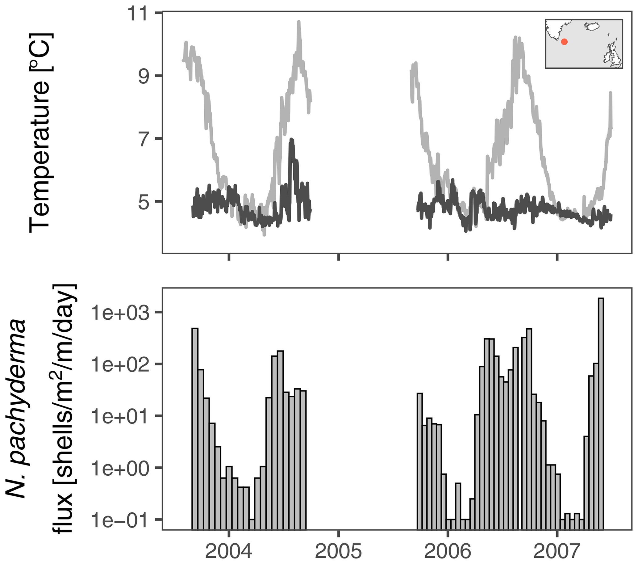
Figure 1Temperature at the surface and at 200–250 m water depth at the Irminger Sea sediment trap mooring (red dot in map inset). In winter and spring the water column is mixed to great depths. The bottom panel shows the evolution of the shell flux of N. pachyderma (150–250 µm from Jonkers et al. (2010); zero fluxes are shown as 0.1 ); stable isotope data are available for all but the lowest flux intervals (Fig. 2). No data are available for the deployment from 2004 to 2005 because of failure of the sediment trap.
2.2 Data
Stable isotope measurements were performed on groups of four N. pachyderma shells (150–250 µm) with up to six measurements per collection interval. In Jonkers et al. (2010) we presented average stable isotope data, but here we return to the raw data and assess the variability within each sample. Even though the measurements were done on groups of four shells, the replicate measurements on small numbers of shells allow us to obtain a first-order estimate of the minimum stable isotope variability within the population of N. pachyderma. Our analyses are therefore meaningful for the interpretation of IFA results. Not all samples from the time series contained enough shells of N. pachyderma (Fig. 1), so the complete dataset consists of 172 measurements from 45 samples, of which 163 are from 36 samples with at least two measurements. All measurements were done using a Thermo MAT253 mass spectrometer coupled to a Kiel IV device. The analytical error (1 SD), determined from repeat measurements of the NBS-19 standard, amounts to 0.05 ‰ for δ18O and 0.03 ‰ for δ13C. Further details about the mooring and the analytical procedures are presented in Jonkers et al. (2010).
The number of replicate measurements per sample is relatively low compared to what is used for IFA on sedimentary material. This is however justified given the short collection intervals of sediment trap samples (in our case 16–19 d) compared to the long integration time of sediment samples (at least decades to centuries). Moreover, with low numbers of measurements we are likely to underestimate the variability at population level, and our inferences will therefore be conservative.
In order to obtain a conservative estimate of the variability among the measured groups of N. pachyderma shells, we remove possible outliers. Given the small sample sizes, outliers were identified using all data in Fig. 2 and excluded from our analysis to avoid unnecessary inflation of inter-specimen variability. We calculated the residual from the mean for each sample and defined outliers as being more than 1.5 times the interquartile range away from the overall mean (Fig. 3). This approach resulted in the removal of 10 (6 %) and 4 (2 %) measurements of δ18O and δ13C respectively.
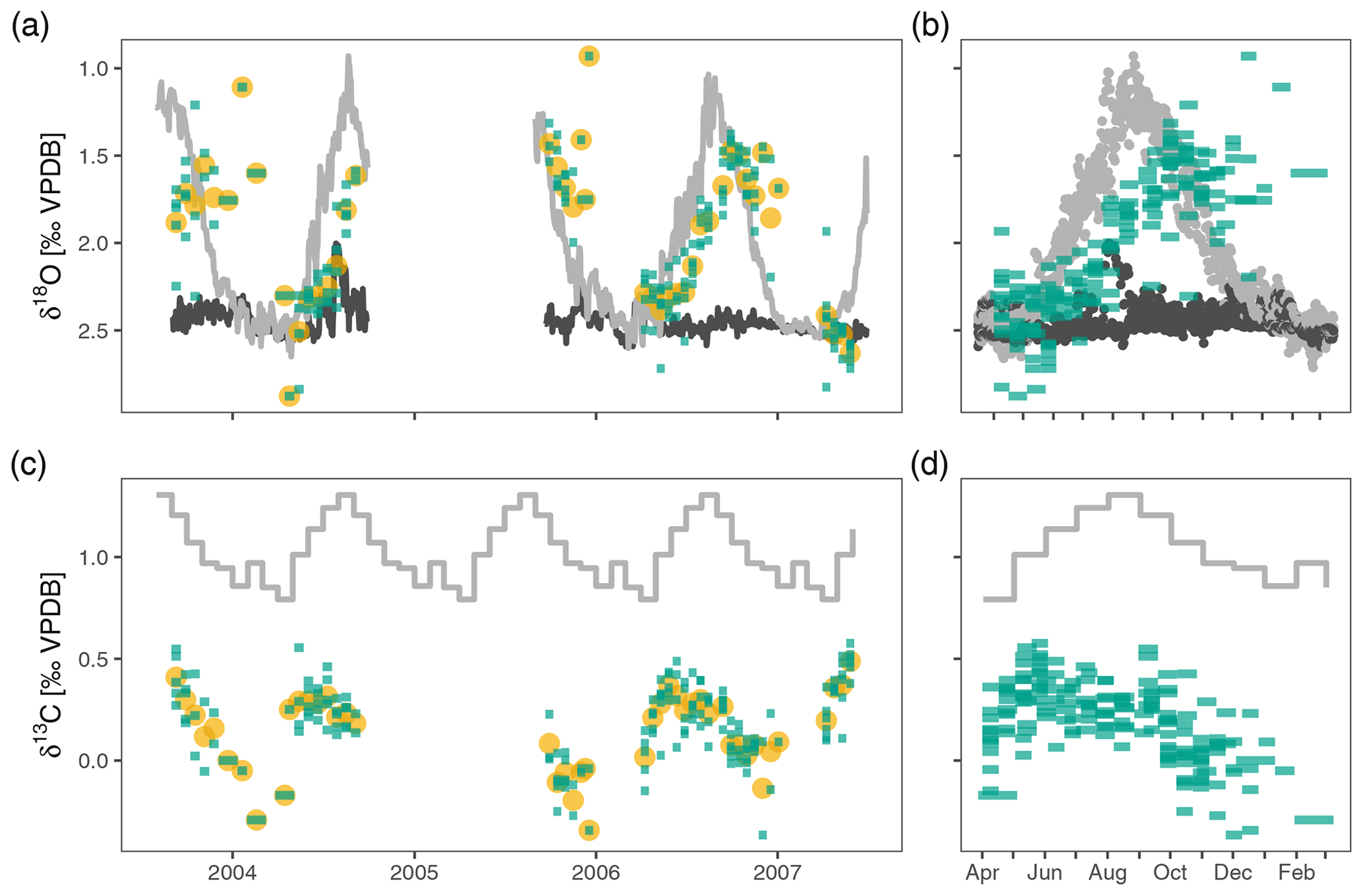
Figure 2Neogloboquadrina pachyderma stable isotopes in the Irminger Sea sediment trap time series. Panels (a) and (c) show the time series of δ18O and δ13C respectively. Panels (b) and (d) highlight the annual pattern; they show the same data collapsed onto a single year. Green bars extend over the collection interval and show individual measurements for groups of four shells; yellow points are average values per sample. The light grey lines depict surface δ18Oeq and δ13CDIC; dark grey lines in (a) and (b) are δ18Oeq at 200–250 m depth. The oxygen and carbon isotopes show considerable variability within each sample, also when the water column is mixed in April–May, suggesting stable isotope variability in excess of what can be explained based on environmental variability alone. The average oxygen isotope ratios track the seasonal cycle of near-surface δ18Oeq (light grey line in a and b) with an offset due to a slightly deeper calcification depth and/or a delay. Stable carbon isotopes also show a clear seasonal cycle, but with a marked offset from the δ13C of DIC (grey line in c and d).
We compare the observations to expected δ18O equilibrium values and estimates of the δ13C of dissolved inorganic carbon (δ13CDIC). We calculate equilibrium δ18O (δ18Oeq) using the Kim and O'Neil (1997) palaeo-temperature equation because N. pachyderma calcifies without an offset from this equation (Jonkers et al., 2010, 2013). For the deployments from 2003–2004 and 2005–2006 we use the same temperature and salinity data as in previous work (Jonkers et al., 2010, 2013). However, for the deployment from 2006–2007 temperature and salinity data at 10 and 266 m are available from the nearby CIS mooring (59.66∘ N, 39.66∘ W), and we use these as it allows use of in situ surface salinity measurements and because of better temporal coverage at depth (Jonkers et al., 2016). Seawater δ18O (δ18Oseawater) was derived from salinity, using the regional salinity–δ18Oseawater relationship used in Jonkers et al. (2010).
Estimates of δ13CDIC are the same as in Jonkers et al. (2013) and based on multiple-linear regression of temperature, salinity and nutrients within the wider subpolar North Atlantic. Since the δ13CDIC data are derived from data that represent long-term average conditions (climatology), they cannot be used to the same level of detail as δ18O. We compare the measured variability in δ13C to the seasonal range in δ13CDIC and the seasonal range in expected foraminifera δ13C by taking into account a temperature-dependent offset from δ13CDIC (Jonkers et al., 2013).
2.3 Predicting N. pachyderma δ18O variability
Planktonic foraminifera intermittently add chambers during their life cycle and start sinking towards the ocean floor upon death. The signal contained in their stable isotope ratios is therefore a reflection of the environmental conditions during a certain time prior to arrival in the sediment trap. To assess if the observed variability in δ18O can be explained by temperature and δ18Oseawater alone, we predict δ18O calcite (δ18Oequilibrium) using a model that is more complex in its representation of calcification than what is usually attempted when interpreting results of individual foraminifera analyses (Glaubke et al., 2021; Groeneveld et al., 2019; Thirumalai et al., 2013). We simulate foraminifera δ18O as an average of individual chamber δ18O and add a delay between formation of the final chamber and arrival at the sediment trap that reflects time spent in the water column without calcification and sinking to the depth of the trap. In this way we represent calcification during the foraminifera life cycle more realistically and allow for more variability than when assuming that each foraminifera shell represents environmental conditions averaged over 1 (calendar) month. Our approach is based on the following assumptions: (1) foraminifera build their chambers at random times during their life cycle, (2) chamber formation takes 1 d (day), (3) each foraminifera shell consists of four chambers with equal mass and (4) all shells have the same mass.
The first assumption is reasonable in light of the limited amount of information available on the (temporal aspects of the) ontogeny of N. pachyderma (Bé et al., 1979; Spindler, 1996). The assumed duration of chamber formation is based on culture studies (Bé et al., 1979; Spindler, 1996). However, culture studies in the closely related species N. dutertrei have shown that chamber formation may take up to 4 d (Fehrenbacher et al., 2017). Longer chamber formation could in theory reduce the variability of foraminifera δ18O because of increased smoothing of the environmental signal. In practice this effect is however negligible because of strong temporal autocorrelation in the δ18Oequilibrium time series that renders the effect of smoothing of up to 4 d insignificant. Our approach thus yields an estimate of variability that is robust against the likely range of chamber formation duration. In N. pachyderma the last whorl of the shell makes up most of the mass and generally consists of four chambers that are of similar size. The assumed number and equal mass of the chambers is thus reasonable. The last assumption is out of convenience.
For each sample we simulate δ18O for different calcification spans (the time it takes to form a four-chambered synthetic shell) and delays (the time between formation of the last chamber and arrival at the trap). We vary the calcification span between 4 and 168 d and the delay between 5 and 180 d. The minimum value for the delay is based on estimates of sinking velocity of planktonic foraminifera (Takahashi and Bé, 1984). We exclude scenarios where the sum of calcification span and delay is more than 181 d because of the clear seasonal pattern in mean δ18O. This pattern indicates that long delays are unlikely because minimum δ18O values are observed shortly after peak temperatures. Very long calcification spans are also unlikely as these would result in small seasonal δ18O variation. We allow for some variability in the calcification span and delay by varying the calcification span in each scenario within a lognormal distribution, with the mode equal to the calcification span and a standard deviation of 0.3. The delay is varied using a normal distribution with a standard deviation that is the square root of the delay.
To investigate the effect of calcification depth, we run two groups of simulations, one where we assume that calcification takes place exclusively at the surface and another where we allow for variable calcification depth, either near the surface or at depth (ca. 250 m), within each sample. We include the possibility that shells were formed at depth because N. pachyderma is known to inhabit a wide depth range (Greco et al., 2019), and previous studies indicated a large and variable apparent calcification depth (Kohfeld et al., 1996; Simstich et al., 2003). However, the real range of apparent calcification depth of N. pachyderma in the Irminger Sea is probably narrower than the 200–250 m assumed in the simulations. This is because the average δ18O of N. pachyderma shows a seasonal trend with a magnitude that suggests an apparent calcification depth around 50 m (Jonkers et al., 2010, 2013). This scenario thus likely overestimates variability, especially during the summer season when the water column is stratified. We do not simulate calcification exclusively at depth because this is clearly at odds with observed seasonal amplitudes of δ18O and δ13C.
We do not consider the possibility of ontogenetic vertical migration in our simulations. This is partly an assumption out of necessity because we do not have temperature and salinity data between the surface and 200 m depth for the entire time series. We however stress that our approach is conservative because ontogenetic migration would decrease the variability in foraminifera stable isotope ratios.
To be consistent with the measurements on groups of four shells, we average the δ18O of four simulated shells. We add measurement uncertainty (white noise with a standard deviation of 0.05 ‰) to the averaged δ18O and calculate the standard deviation of the δ18O of two to six groups (depending on the sample) of four shells. We repeated this process 300 times for each sample and for each combination of delay and calcification span. We consider cases significant when the predicted standard deviation is higher than the observed standard deviation in 95 % of the simulations.
Estimates of δ18Oequilibrium are not available for the entire time series, and our simulations are therefore restricted to the spring of 2004, the spring to autumn of 2006 and the spring of 2007. Because we lack detailed data on δ13CDIC, we did not simulate foraminifera δ13C. We, however, do not ignore foraminifera δ13C in our analysis.
Modelling is by definition a simplification of reality. Even though important aspects of our model (variable depth, faster calcification) yield estimates of expected variability that are higher than in previous work, we follow previous work and consider local temperature and δ18Oseawater as the only predictors of δ18Oequilibrium (Glaubke et al., 2021; Thirumalai et al., 2013). For simplicity we do not consider advection of foraminifera because it is not directly clear how advection within the Irminger Gyre, where temperatures are spatially rather uniform, would influence the temperature variability that planktonic foraminifera would be exposed to during calcification. Assessing the influence of advection can only be done using Lagrangian modelling (van Sebille et al., 2015) and ultimately relies on the accuracy with which the model captures spatial and temporal temperature variability. Such modelling is beyond the scope of this study. We also do not consider the effect of the carbonate ion concentration () on foraminifera stable isotopes (Spero et al., 1997). Because of the positive correlation between temperature and (Jonkers et al., 2013) and a negative correlation between and foraminifera δ18O (Spero et al., 1997), the effect would slightly increase the seasonal range δ18Oequilibrium. Assuming that the sensitivity of N. pachyderma δ18O is similar to that of G. bulloides, the increase would be on the order of 0.15 ‰. Since we do not consider this possible source of variability, our simulations are likely to provide conservative estimates of foraminifera δ18O variability.
3.1 Raw data
The δ18O of N. pachyderma varies between 0.93 ‰ in early winter 2006 and 2.88 ‰ in spring 2004 (Fig. 2). The overall seasonal amplitude is around 1 ‰, with a minimum in δ18O that lags the maximum temperatures by 1 to 2 months. Stable oxygen isotope ratios are in general within the range of predicted δ18Oequilibrium. The δ13C values show a smaller amplitude (−0.37 ‰ to 0.58 ‰) and are always offset from δ13CDIC (Fig. 2). The δ13C values generally decrease from spring to winter. For both δ18O and δ13C the observed within-sample variability exceeds the analytical uncertainty (Fig. 3).
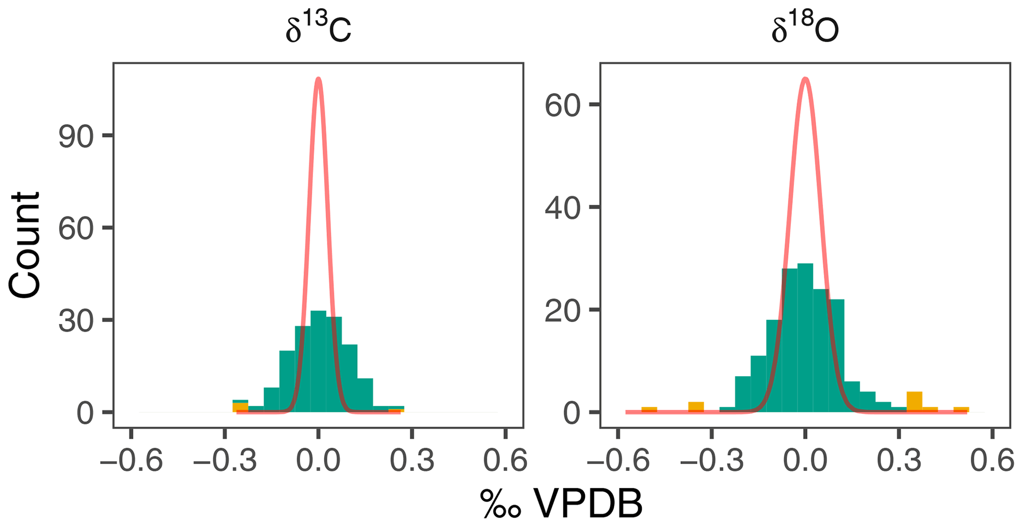
Figure 3Within-sample variability in N. pachyderma stable isotopes exceeds analytical noise. Histograms of residual δ18O and δ13C compared to expected density distribution if variability were due to analytical uncertainty alone (red line). Yellow colours indicate outliers (see methods).
After outlier removal, the within-sample range of δ18O varies between 0.05 ‰ and 0.51 ‰ (mean 0.24 ‰) and does not show a consistent pattern during the year (Fig. 4). There is no relationship between the number of measurements within a sample and the range in δ18O (Fig. 4). The within sample range is always smaller than the seasonal range in surface δ18Oequilibrium. Most of the time the observed δ18O range is also smaller than the vertical gradient in δ18Oequilibrium, except during isothermal conditions in spring when it exceeds the δ18Oequilibrium range (Fig. 4). The range in δ13C is similar to δ18O and varies between 0.06 ‰ and 0.46 ‰ (mean 0.21 ‰) and also does not show a clear seasonal pattern (Fig. 4). Compared to δ18O, the range of foraminifera δ13C is more often above the expected range (Fig. 4).
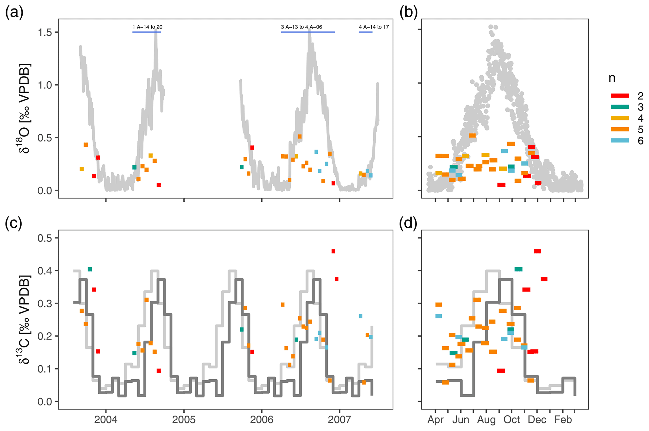
Figure 4The within-sample stable isotope range of N. pachyderma exceeds expected variability in spring when water column conditions are homogeneous and show no consistent seasonal pattern. Note difference scales for δ18O and δ13C. Bars extend to the collection intervals, and colours indicate number of measurements per sample. Grey colours in (a) and (b) depict the difference in δ18O between the surface and 200–250 m water depth. Light grey lines in (c) and (d) show the seasonal range in δ13CDIC and dark grey lines the seasonal range in foraminifera δ13C calculated using a temperature-dependent offset from δ13CDIC (see methods). Samples for which the δ18O variability is simulated (Fig. 5) are indicated in (a).
There are two important points regarding these initial observations. The first is that the observed range in foraminifera stable isotope values exceeds the expected range in spring (April–May) when the water column is well-mixed down to 800 m depth. This variability arises from apparently random positive and negative offsets from δ18Oequilibrium, suggesting that it does not result from a mechanism that would cause a systematic bias in the foraminifera δ18O. Advection or long foraminifera lifespans, which could theoretically cause foraminifera from the previous summer to survive until spring, are therefore unlikely to provide a full explanation for the observed variability. This is the first indication that the variability in foraminifera isotope ratios does not solely result from environmental variability. The second observation is the apparent lack of a seasonal cycle in the range in δ18O and δ13C even though stratification develops as the sea surface warms. In theory, the variability in foraminifera stable isotope ratios could therefore increase towards the warm season. The fact that this cannot be seen in the data indicates that N. pachyderma calcifies in a relatively narrow and constant vertical range.
3.2 Predicted foraminifera δ18O variability
To assess if observed variability in δ18O of N. pachyderma is higher than the variability expected from temperature and δ18O of seawater at the time of sampling because the foraminifera calcified prior to the sampling, we carried out simulations using a range of possible calcification spans and delays. These simulations indicate that the standard deviation of N. pachyderma δ18O in spring when the water column is virtually isothermal (IRM-1 A-14, IRM-3 A-13, IRM-3 A-14, IRM-4 A-14 and IRM-4 A-15) exceeds what can be expected based on reasonable calcification histories and delays (Fig. 5). The predicted variability only significantly exceeds the observations during summer and almost exclusively in the simulations that allow variable calcification depth. Our simulations are thus sensitive to the choice of calcification depth, and it is important to assess if the scenario with variable depth habitat is more realistic than the scenario with constant, near-surface habitat. We can compare both scenarios by determining the prediction error in the mean δ18O across all samples (Fig. 6). The minimum prediction error is, in both scenarios, distributed along an arc shape, with lower errors at longer calcification spans and delays up to about a month or at short calcification spans and delays on the order of 1 to 2 months. However, the errors reach markedly lower values in the scenario where calcification only occurs near the surface. Because the seasonal peak in temperature is reached earlier at the surface than at depth, it remains difficult to determine precisely which combination of calcification depth, calcification span and delay is most realistic, but the amplitude of the mean seasonal δ18O indicates that the surface-only scenario is closer to what the foraminifera actually experienced than the variable depth scenario. This indicates that even when taking reasonable calcification histories and delays into account, the observed variability in foraminifera δ18O is unlikely to reflect environmental (temperature) variability alone.
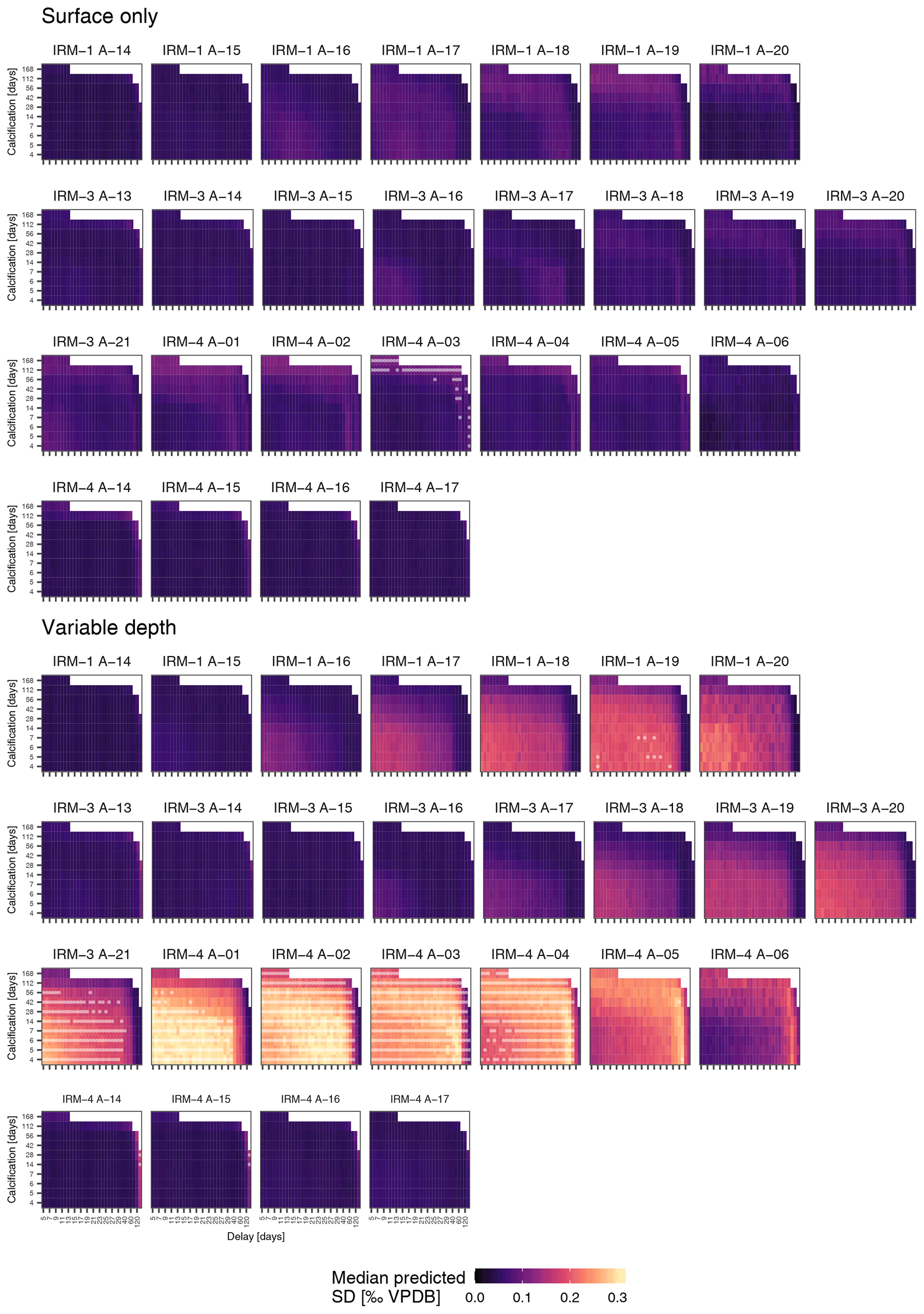
Figure 5Observed δ18O variability in N. pachyderma generally exceeds expectations. Simulated δ18O variability as a function of calcification span and delay for the surface-only and variable-depth scenarios for each sample indicated in Fig. 4. White dots indicate scenarios where the simulated variability significantly exceeds the observed variability; note that this only occurs when a variable calcification depth is assumed. Samples are ordered by year (with two rows for the 2005–2006 period), such that springtime samples are shown on the left. Note that for clarity x-axis ticks and labels are only shown for every second tick; all steps are shown in Fig. 6.
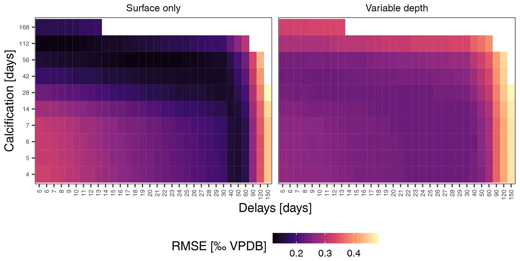
Figure 6Mean foraminifera δ18O constrains simulations. Prediction errors for sample mean δ18O reach markedly lower values for the surface-only simulations, indicating that this scenario is more likely to characterise N. pachyderma in the Irminger Sea. This means that the observed variability (Fig. 4) is unlikely a reflection of temperature and δ18Oseawater variability alone and that the δ18O of individual N. pachyderma shells is not a precise indicator of environmental conditions during calcification.
Our simulations also permit us to put some constraints on the calcification span and delay that characterises N. pachyderma at this location. The hardest constraints can be put on the possibility of long delays between formation of the last chamber and arrival at the trap. Sinking speed measurements suggest that the delay due to sinking at this location is likely to be between 5 and 19 d (Takahashi and Bé, 1984). We obtain minimum prediction errors for delays up to approximately 2 months (Fig. 6). Subtracting the sinking time estimates from these delays implies that N. pachyderma is unlikely to spend more than 1 month in the water column without calcifying after the last chamber has formed. This means that the simulations with delays >100 d are not realistic.
Our simulations indicate that calcification spans under 2 weeks yield smaller errors when associated with delays on the order of 30–60 d, and similarly low prediction errors are obtained using longer calcification spans and shorter delays. Based on our data it is difficult to ascertain which cases are more realistic. However, such long delays would require long intervals spent in the water column without calcification. A single culture study using Antarctic N. pachyderma showed intermittent chamber formation over a period of about 2 months and a single case of gametogenesis approximately 2 weeks after the formation of the final chamber (Spindler, 1996). Other studies also suggest an approximately 2-month lifespan (Davis et al., 2017, 2020a). This suggests that delays of up to approximately 1 month (including settling) and calcification of the final four chambers over the course of about 2 months are most probable.
3.3 Excess foraminifera δ18O variability
The mean observed standard deviation for of δ18O is 0.11±0.05 ‰ for the complete time series and 0.10±0.03 ‰ for the samples from the time when the water column was isothermal (IRM-1 A-14, IRM-3 A-13, IRM-3 A-14, IRM-4 A-14 and IRM-4 A-15). As noted above, the fact that the variability in δ18O does not show a consistent pattern during the year suggests that we have captured the full range of within-sample variability even though the number of measurements per sample is relatively low. Since our measurements are based on groups of four shells, the observed standard deviation is an underestimate of the standard deviation among individual shells. Assuming that each shell in the group contributed equally to the total mass, the degree of underestimation of the standard deviation scales with the square root of the group size (Groeneveld et al., 2019). Thus we multiply the observed standard deviation by 2 () to obtain an estimate of the standard deviation of individual shells. That means that the δ18O of individual foraminifera at this location is likely to have a standard deviation of 0.19±0.07 ‰ (0.21±0.11 ‰ when considering all observations).
For the samples from the times when the water column was deeply mixed, i.e. when variations in temperature, salinity and hence δ18Oequilibrium were negligible, our simulations predict a standard deviation for individual shells of 0.08 ‰. This prediction is identical for both depth scenarios. It includes a 0.05 ‰ measurement uncertainty and is based on all considered scenarios with a delay less than 100 d, which is reasonable given the low model skill at longer delays. Assuming that our simulations are a reasonable approximation of reality, the excess variability (SD) that cannot be explained by variability in temperature and δ18Oseawater is therefore 0.11±0.06 ‰, which in terms of temperature roughly translates to a standard deviation of 0.4 ∘C.
Whereas our modelling approach provides an estimate that is likely closer to reality than assuming that foraminifera reflect environmental conditions averaged over a single (calendar) month, our estimate could be evaluated by simulating other calcification trajectories. We found that our results are insensitive to the duration of chamber formation. Experiments where we allowed complete shell formation within 1 d, equivalent to assigning all weight to the last chamber, yielded an expected standard deviation of individual foraminifera δ18O of 0.09 ‰. Therefore, the assumption of equal weight of the four chambers has little bearing on our results. Ultimately, the modelled foraminifera δ18O depends on the hydrographic data used to estimate δ18Oequilibrium. By using data from the surface and from great depth, we have obtained two end-member scenarios of vertical δ18Oequilibrium variability that implicitly encompass ontogenetic vertical migration. However, future estimates of expected individual foraminifera δ18O variability could be improved by explicitly incorporating horizontal δ18Oequilibrium variability and advection during shell growth in the modelling strategy.
Apart from being sensitive to our modelling design and data availability, our estimate of excess δ18O variability among individual shells is also sensitive to the quantification of variability among shells. To obtain a conservative estimate, we excluded potential outliers. Were we to consider all measurements, the average standard deviation among groups would be 0.15±0.11 ‰ (0.17±0.09 ‰ during spring) and the resulting excess δ18O variability 0.25±0.19 ‰. Thus our approach yields a conservative and better constrained estimate of the excess variability.
We compare this estimate of unexplained δ18O variability to two studies that used individual foraminifera δ18O from cores in the eastern equatorial Pacific Ocean to infer changes in the El Niño–Southern Oscillation. In the first study, the range in the standard deviations of N. dutertrei δ18O shells in eight time slices across the past 50 000 years amounts to 0.15 ‰ (Leduc et al., 2009). In the second study, Rustic et al. (2015) interpreted changes in the standard deviation of G. ruber δ18O over the last millennium that were smaller than 0.45 ‰ (variance of 0.20 ‰). Forward modelling studies also indicate that changes in the amplitude (doubling or halving) in the central equatorial Pacific would translate to changes in the standard deviation of IFA of maximum 0.15 ‰ (Thirumalai et al., 2013). In all cases, the unexplainable δ18O variability we observe makes up a substantial part of the signal. Thus, non-temperature effects on individual foraminifera δ18O need to be considered when interpreting the results of IFA.
3.4 Possible causes of excess variability
The relatively constant variability in δ18O and δ13C within the N. pachyderma population in the Irminger Sea during the year argues against a direct environmental influence on the variability. This is because on seasonal timescales environmental variability is strongly correlated to temperature and/or stratification. The observed variability could therefore be random or reflect biological processes within the population of foraminifera, where each shell, or each chamber, records the environment with a small offset. As long as the excess variability remains random or uncorrelated with the environment, the average stable isotope composition of (large enough subsample of) a foraminifera population will accurately reflect environmental conditions. On a population level, planktonic foraminifera δ18O is indeed a reliable indicator of seawater temperature and δ18Oseawater (e.g. Bemis et al., 1998; Erez and Luz, 1982), suggesting that the excess variability among individual specimens is cancelled out within populations.
Alternatively, the excess variability could arise from environmental or biotic forcing that we did not consider in our simulations. Crucially, any possible mechanism needs to explain the approximately equal variability in δ18O and δ13C that we observe in the time series.
Shell size is likely to affect metabolic rates, and the observed excess variability could therefore be related to differences in shell size (Spero and Lea, 1993, 1996). However, in such a scenario, the effect would be expected to be much stronger on δ13C than on δ18O, as is the case for G. bulloides (Spero and Lea, 1996). The comparable variability in both carbon and oxygen isotope ratios thus suggests that size differences within the foraminifera population are unlikely to explain the observed excess variability.
Along similar lines, growth rate may vary among individual foraminifera and thereby influence the stable isotope composition, as has for instance been shown for corals (McConnaughey, 1989). However, in corals, δ13C is, like with the size effect above, more sensitive to changes in the growth rate than δ18O. Therefore, if such an effect were to occur among (non-symbiotic) planktonic foraminifera, growth rate differences would also not be the likely cause of the excess variability in stable isotope ratios.
The excess variability could also arise from differences in the proportion of crust to lamellar calcite. We did not perform a systematic analysis of the degree of encrustation of N. pachyderma in the sediment trap samples, but in the many years of work on this time series we have never come across a crust-free specimen. It is likely that the degree of encrustation varies among individuals, and variable crust-to-lamellar calcite ratios among foraminifera could therefore add temperature-independent noise, similar to what has been suggested for MgCa (Jonkers et al., 2016, 2021). However, the difference between crust and lamellar calcite δ18O of N. pachyderma intercepted in spring when the water column was well-mixed is not significant (Livsey et al., 2020). Variable encrustation can therefore not be the explanation for the excess δ18O variability observed during the isothermal conditions in spring. In addition, this explanation would require that the crust and lamellar calcite also have different carbon isotope ratios. However, previous work is inconclusive in this regard. Observations from plankton hauls suggest that encrusted and crust-free N. pachyderma have systematically different δ13C, but that the effect of encrustation is not as strong as on δ18O (Kohfeld et al., 1996). A larger dataset from the sediment on the other hand indicates no effect of encrustation (Healy-Williams, 1992). Whether or not variable encrustation is the cause of the observed excess variability in δ18O and δ13C therefore remains an open question.
Notwithstanding the fact that the exact cause of the excess variability in N. pachyderma stable isotope ratios needs to be constrained in future studies, our analysis shows that individual planktonic foraminifera record environmental conditions with less precision than average populations. Our study thus confirms earlier indications (Groeneveld et al., 2019; Livsey et al., 2020), but we have attempted a first quantification of this noise for δ18O, which has up to now been ignored in the interpretation of individual foraminifera data.
3.5 Implications for reconstructions of environmental variability based on individual foraminifera
The possibility that individual planktonic foraminifera record seawater conditions with limited precision has up to now been overlooked when using the geochemistry of individual planktonic foraminifera to reconstruct climate variability. Our analyses provide evidence that the δ18O of individual N. pachyderma shells may reflect seawater temperature and δ18O with a precision of only 0.11 ‰. For now we assume that the cause of this lack of precision is random biological noise, but future studies are needed to verify that this is indeed the case, or if the recording precision is dependent on environmental or biological factors.
Our observations strengthen the case to use large numbers of foraminifera, not just for IFA. Depending on instrumental precision, the biological recording noise doubles or triples the variability that can be expected in (individual) planktonic foraminifera δ18O, even when temperatures were constant during calcification. Any study using individual foraminifera δ18O to infer past environmental variability thus needs to cross this noise threshold in order to obtain meaningful results. Lack of recording precision will also influence the shape of the distribution of IFA results (Fig. 7), especially at the tails of the distribution that are often used to infer changes in upper ocean dynamics (Glaubke et al., 2021).
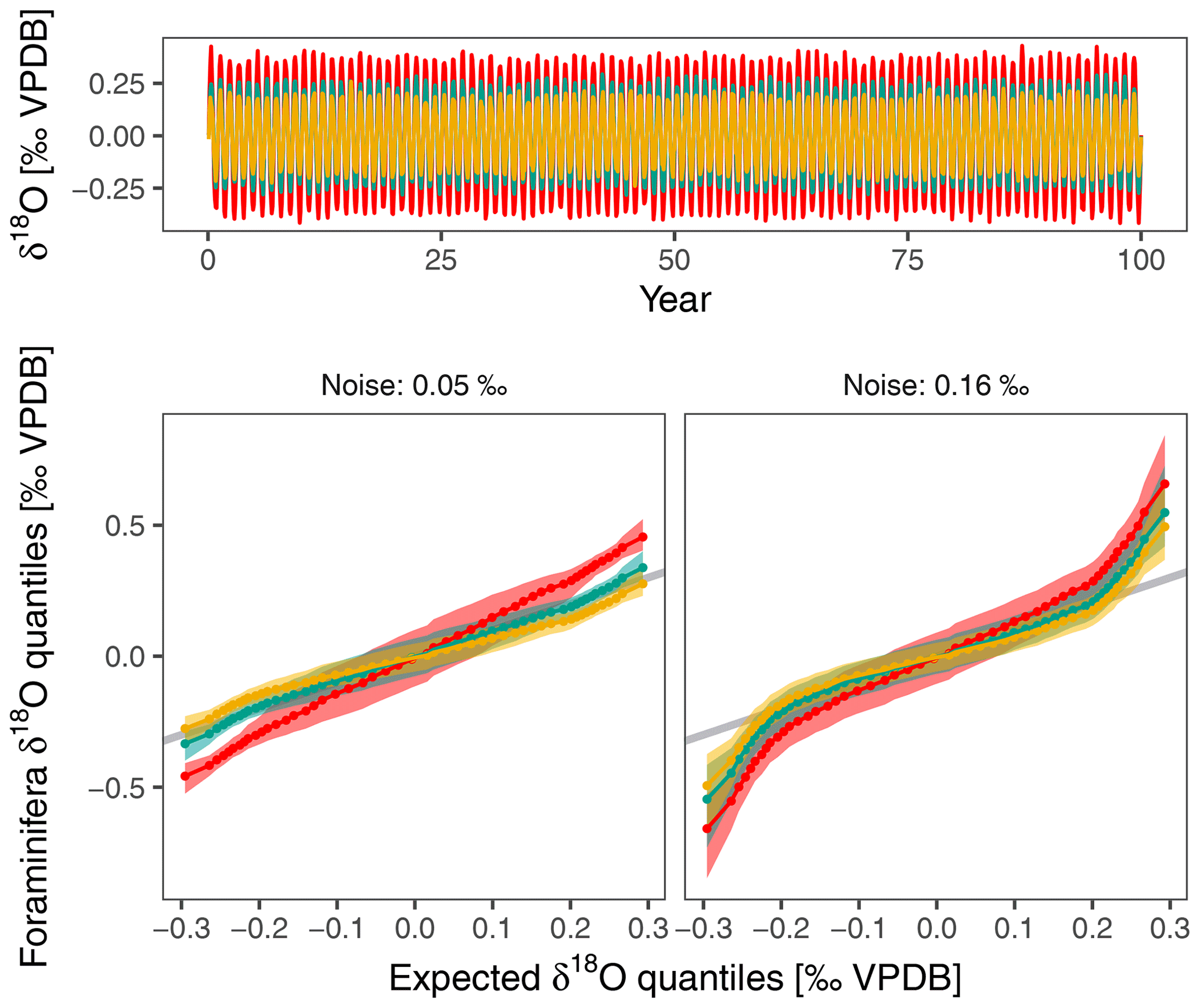
Figure 7Excess δ18O variability mostly affects tails of δ18O distribution within individual foraminifera. This simple simulation shows the effect of excess variability on capability to reconstruct changes in the amplitude of the seasonal cycle. The input consists of a synthetic δ18Oeq time series with a seasonal amplitude of 0.25 ‰ that is not atypical of conditions in the central equatorial Pacific. The monthly time series is constructed using a sine wave with 0.02 ‰ random noise and is sampled 100 times at random to crudely represent planktonic foraminifera δ18O. This is an optimistic scenario as fewer foraminifera are usually used for IFA. The Q–Q plots show the effect of a change in the seasonal amplitude of δ18Oeq for a scenario that only accounts for analytical noise (assumed to be 0.05 ‰) and for another that incorporates the excess variability found in this study. Higher noise levels affect the tails of the distribution and make it harder to detect changes in the seasonality.
There are no reasons to believe that the existence of biological recording noise is unique to N. pachyderma or to stable oxygen and carbon isotopes alone. In fact, most of the indications for excess variability are based on other species (Bemis et al., 1998; Erez and Luz, 1982; Leduc et al., 2009; Spero and Lea, 1996). We therefore presume that a similar noise characterises other species and proxies as well. However, more research is needed to constrain the nature and causes of this lack of precision in the recording by individual foraminifera. Future research, including culturing, needs to consider different species in different environmental settings. Including MgCa as an independent temperature-sensitive parameter may also help to elucidate the cause of the excess variability. Notwithstanding, our data clearly show that the assumption that individual planktonic foraminifera are perfect recorders of (monthly mean) temperature is not valid. Biology cannot be ignored in the interpretation of planktonic foraminifera proxies.
Stable isotope measurements on groups of four shells of N. pachyderma from a 16–19 d resolution sediment trap time series in the subpolar North Atlantic show large within sample variability. Stable oxygen and carbon isotope ratios within the time series have a mean standard deviation of 0.11 ‰ and 0.10 ‰ respectively and show no relationship with the seasonal trend in temperature (δ18Oeq) or the δ13C of dissolved inorganic carbon. This lack of a seasonal pattern in the variability suggests that at this location N. pachyderma has a seasonally rather stable apparent calcification depth, which based on the amplitude of the sample mean δ18O is around 50 m.
Due to deep mixing, the site is characterised by homogeneous water column conditions at the start of the spring foraminifera flux pulse. Neogloboquadrina pachyderma stable isotope variability at this time exceeds the variability that can be expected from the local hydrography, indicating an additional source of variability that has so far not been considered in the interpretation of records of the geochemistry of individual foraminifera. Predictions of the observed variability in N. pachyderma δ18O from temperature and δ18Oseawater using realistic calcification and settling histories fail to match the observed variability. We therefore conclude that the δ18O of individual N. pachyderma imperfectly record temperature and δ18Oseawater. Whether random, or controlled by environmental or biological factors, N. pachyderma records environmental variability with some degree of noise.
Our first-order estimate of the recording noise of individual specimens amounts to 0.11 ‰ (1 SD), which is approximately double the typical analytical noise. Whilst more studies are needed to constrain the origin and variability in this recording noise, there are no reasons to believe it is a feature exclusive to N. pachyderma. Recording noise should therefore be considered when interpreting geochemical variability among individual foraminifera.
The stable isotope data have been submitted to http://pangaea.de (last access: January 2022).
LJ conceived the study and analysed the data. LJ formulated the model with feedback from JM. GJB initiated the Irminger Sea sediment trap moorings and organised the funding. LJ led the writing of the paper and created the figures. All authors reviewed and edited the paper.
The contact author has declared that neither they nor their co-authors have any competing interests.
Publisher's note: Copernicus Publications remains neutral with regard to jurisdictional claims in published maps and institutional affiliations.
We would like to thank the two anonymous reviewers who provided valuable feedback on an earlier version of this article. The CIS mooring temperature and salinity data were collected and made freely available by the OceanSITES project (http://www.oceansites.org, last access: 14 April 2015) and the national programmes that contribute to it.
Lukas Jonkers received funding through the German climate modelling initiative
PALMOD, funded by the German Ministry of Science and Education (BMBF). Julie Meilland
is funded by the Cluster of Excellence “The Ocean Floor –
Earth's Uncharted Interface” funded by the German Research Foundation
(DFG).
The deployment of the sediment trap moorings was funded by NWO within the VAMOC (RAPID) programme (grant
854.00.020).
The article processing charges for this open-access publication were covered by the University of Bremen.
This paper was edited by Marit-Solveig Seidenkrantz and reviewed by two anonymous referees.
Bé, A. W. H., Hemleben, C., Anderson, O. R., and Spindler, M.: Chamber formation in planktonic foraminifera, Micropaleontology, 25, 294–307, 1979.
Bemis, B. E., Spero, H. J., Bijma, J., and Lea, D. W.: Reevaluation of the Oxygen Isotopic Composition of Planktonic Foraminifera: Experimental Results and Revised Paleotemperature Equations, Paleoceanography, 13, 150–160, 1998.
Davis, C. V., Fehrenbacher, J. S., Hill, T. M., Russell, A. D., and Spero, H. J.: Relationships Between Temperature, pH, and Crusting on MgCa ratios in Laboratory-Grown Neogloboquadrina Foraminifera, Paleoceanography, 32, 1137–1152, https://doi.org/10.1002/2017PA003111, 2017.
Davis, C. V., Livsey, C. M., Palmer, H. M., Hull, P. M., Thomas, E., Hill, T. M., and Benitez-Nelson, C. R.: Extensive morphological variability in asexually produced planktic foraminifera, Science Advances, 6, eabb8930, https://doi.org/10.1126/sciadv.abb8930, 2020a.
Davis, C. V., Fehrenbacher, J. S., Benitez-Nelson, C., and Thunell, R. C.: Trace Element Heterogeneity Across Individual Planktic Foraminifera from the Modern Cariaco Basin, J. Foramin. Res., 50, 204–218, 2020b.
Dueñas-Bohorquez, A., da Rocha, R. E., Kuroyanagi, A., de Nooijer, L. J., Bijma, J., and Reichart, G.-J.: Interindividual variability and ontogenetic effects on Mg and Sr incorporation in the planktonic foraminifer Globigerinoides sacculifer, Geochim. Cosmochim. Ac., 75, 520–532, 2011.
Elderfield, H. and Ganssen, G.: Past temperature and δ18O of surface ocean waters inferred from foraminiferal MgCa ratios, Nature, 405, 442–445, 2000.
Erez, J. and Luz, B.: Temperature control of oxygen-isotope fractionation of cultured planktonic foraminifera, Nature, 297, 220–222, 1982.
Fehrenbacher, J., Marchitto, T., and Spero, H. J.: Comparison of laser ablation and solution-based ICP-MS results for individual foraminifer MgCa and SrCa analyses, Geochem. Geophy. Geosy., 21, e2020GC009254, https://doi.org/10.1029/2020gc009254, 2020.
Fehrenbacher, J. S., Russell, A. D., Davis, C. V., Gagnon, A. C., Spero, H. J., Cliff, J. B., Zhu, Z., and Martin, P.: Link between light-triggered Mg-banding and chamber formation in the planktic foraminifera Neogloboquadrina dutertrei, Nat. Commun., 8, 15441, https://doi.org/10.1038/ncomms15441, 2017.
Ganssen, G. M., Peeters, F. J. C., Metcalfe, B., Anand, P., Jung, S. J. A., Kroon, D., and Brummer, G.-J. A.: Quantifying sea surface temperature ranges of the Arabian Sea for the past 20 000 years, Clim. Past, 7, 1337–1349, https://doi.org/10.5194/cp-7-1337-2011, 2011.
Glaubke, R. H., Thirumalai, K., Schmidt, M. W., and Hertzberg, J. E.: Discerning changes in high-frequency climate variability using geochemical populations of individual Foraminifera, Paleoceanography and Paleoclimatology, 36, e2020PA004065, https://doi.org/10.1029/2020pa004065, 2021.
Greco, M., Jonkers, L., Kretschmer, K., Bijma, J., and Kucera, M.: Depth habitat of the planktonic foraminifera Neogloboquadrina pachyderma in the northern high latitudes explained by sea-ice and chlorophyll concentrations, Biogeosciences, 16, 3425–3437, https://doi.org/10.5194/bg-16-3425-2019, 2019.
Groeneveld, J., Ho, S. L., Mackensen, A., Mohtadi, M., and Laepple, T.: Deciphering the Variability in MgCa and Stable Oxygen Isotopes of Individual Foraminifera, Paleoceanography and Paleoclimatology, 34, 755–773, 2019.
Haarmann, T., Hathorne, E. C., Mohtadi, M., Groeneveld, J., Kölling, M., and Bickert, T.: MgCa ratios of single planktonic foraminifer shells and the potential to reconstruct the thermal seasonality of the water column, Paleoceanography, 26, PA3218, https://doi.org/10.1029/2010pa002091, 2011.
Healy-Williams, N.: Stable isotope differences among morphotypes of Neogloboquadrina pachyderma (Ehrenberg): implications for high-latitude palaeoceanographic studies, Terra nova, 4, 693–700, 1992.
de Jong, M. F., van Aken, H. M., Våge, K., and Pickart, R. S.: Convective mixing in the central Irminger Sea: 2002–2010, Deep-Sea Res. Pt. I, 63, 36–51, 2012.
Jonkers, L., Brummer, G.-J. A., Peeters, F. J. C., van Aken, H. M., and De Jong, M. F.: Seasonal stratification, shell flux, and oxygen isotope dynamics of left-coiling N. pachyderma and T. quinqueloba in the western subpolar North Atlantic, Paleoceanography, 25, PA2204, https://doi.org/10.1029/2009PA001849, 2010.
Jonkers, L., van Heuven, S., Zahn, R., and Peeters, F. J. C.: Seasonal patterns of shell flux, δ18O and δ13C of small and large N. pachyderma (s) and G. bulloides in the subpolar North Atlantic, Paleoceanography, 28, 164–174, 2013.
Jonkers, L., Buse, B., Brummer, G.-J. A., and Hall, I. R.: Chamber formation leads to MgCa banding in the planktonic foraminifer Neogloboquadrina pachyderma, Earth Planet. Sc. Lett., 451, 177–184, 2016.
Jonkers, L., Gopalakrishnan, A., Weßel, L., Chiessi, C. M., Groeneveld, J., Monien, P., Lessa, D., and Morard, R.: Morphotype and crust effects on the geochemistry of Globorotalia inflata, Paleoceanography and Paleoclimatology, 36, e2021PA004224, https://doi.org/10.1029/2021pa004224, 2021.
Kim, S.-T. and O'Neil, J. R.: Equilibrium and nonequilibrium oxygen isotope effects in synthetic carbonates, Geochim. Cosmochim. Ac., 61, 3461–3475, 1997.
Kohfeld, K. E., Fairbanks, R. G., Smith, S. L., and Walsh, I. D.: Neogloboquadrina pachyderma (sinistral coiling) as Paleoceanographic Tracers in Polar Oceans: Evidence from Northeast Water Polynya Plankton Tows, Sediment Traps, and Surface Sediments, Paleoceanography, 11, 679–699, 1996.
Leduc, G., Vidal, L., Cartapanis, O., and Bard, E.: Modes of eastern equatorial Pacific thermocline variability: Implications for ENSO dynamics over the last glacial period, Paleoceanography, 24, PA3202, https://doi.org/10.1029/2008PA001701, 2009.
Livsey, C. M., Kozdon, R., Bauch, D., Brummer, G.-J. A., Jonkers, L., Orland, I., Hill, T. M., and Spero, H. J.: High-Resolution MgCa and δ18O Patterns in Modern Neogloboquadrina pachyderma From the Fram Strait and Irminger Sea, Paleoceanography and Paleoclimatology, 35, e2020PA003969, https://doi.org/10.1029/2020pa003969, 2020.
McConnaughey, T.: 13C and 18O isotopic disequilibrium in biological carbonates: I. Patterns, Geochim. Cosmochim. Ac., 53, 151–162, 1989.
Metcalfe, B., Lougheed, B. C., Waelbroeck, C., and Roche, D. M.: A proxy modelling approach to assess the potential of extracting ENSO signal from tropical Pacific planktonic foraminifera, Clim. Past, 16, 885–910, https://doi.org/10.5194/cp-16-885-2020, 2020.
de Nooijer, L. J., Hathorne, E. C., Reichart, G. J., Langer, G., and Bijma, J.: Variability in calcitic MgCa and SrCa ratios in clones of the benthic foraminifer Ammonia tepida, Mar. Micropaleontol., 107, 32–43, 2014.
Rustic, G. T., Koutavas, A., Marchitto, T. M., and Linsley, B. K.: Dynamical excitation of the tropical Pacific Ocean and ENSO variability by Little Ice Age cooling, Science, 350, 1537–1541, https://doi.org/10.1126/science.aac9937, 2015.
van Sebille, E., Scussolini, P., Durgadoo, J. V., Peeters, F. J. C., Biastoch, A., Weijer, W., Turney, C., Paris, C. B., and Zahn, R.: Ocean currents generate large footprints in marine palaeoclimate proxies, Nat. Commun., 6, 6521, https://doi.org/10.1038/ncomms7521, 2015.
Simstich, J., Sarnthein, M., and Erlenkeuser, H.: Paired δ18O signals of Neogloboquadrina pachyderma (s) and Turborotalita quinqueloba show thermal stratification structure in Nordic Seas, Mar. Micropaleontol., 48, 107–125, 2003.
Spero, H. J. and Lea, D. W.: Intraspecific stable isotope variability in the planktic foraminifera Globigerinoides sacculifer: Results from laboratory experiments, Mar. Micropaleontol., 22, 221–234, 1993.
Spero, H. J. and Lea, D. W.: Experimental determination of stable isotope variability in Globigerina bulloides: implications for paleoceanographic reconstructions, Mar. Micropaleontol., 28, 231–246, 1996.
Spero, H. J., Bijma, J., Lea, D. W., and Bemis, B. E.: Effect of seawater carbonate concentration on foraminiferal carbon and oxygen isotopes, Nature, 390, 497–500, 1997.
Spindler, M.: On the salinity tolerance of the planktonic foraminifer Neogloboquadrina pachyderma from Antarctic sea ice, in: Proceedings of the NIPR Symposium on Polar Biology, 9, 85–91, 1996.
Takahashi, K. and Bé, A. W. H.: Planktonic foraminifera: factors controlling sinking speeds, Deep-Sea Res. Pt. I, 31, 1477–1500, 1984.
Thirumalai, K., Partin, J. W., Jackson, C. S., and Quinn, T. M.: Statistical constraints on El Niño Southern Oscillation reconstructions using individual foraminifera: A sensitivity analysis, Paleoceanography, 28, 401–412, 2013.