Orbital insolation variations, intrinsic climate variability, and Quaternary glaciations

The relative role of external forcing and of intrinsic variability is a key question of climate variability in general and of our planet's paleoclimatic past in particular. Over the last 100 years since Milankovic's contributions, the importance of orbital forcing has been established for the period covering the last 2.6 Myr and the Quaternary glaciation cycles that took place during that time. A convincing case has also been made for the role of several internal mechanisms that are active on timescales both shorter and longer than the orbital ones. Such mechanisms clearly have a causal role in Dansgaard–Oeschger and Heinrich events, as well as in the mid-Pleistocene transition. We introduce herein a unified framework for the understanding of the orbital forcing's effects on the climate system's internal variability on timescales from thousands to millions of years. This framework relies on the fairly recent theory of non-autonomous and random dynamical systems, and it has so far been successfully applied in the climate sciences for problems like the El Niño–Southern Oscillation, the oceans' wind-driven circulation, and other problems on interannual to interdecadal timescales. Finally, we provide further examples of climate applications and present preliminary results of interest for the Quaternary glaciation cycles in general and the mid-Pleistocene transition in particular.

1 Introduction and motivation

In the early 20th century, Milutin Milankovic presented his theory of ice ages (Milankovitch, 1920). Based on his own calculations and on insightful suggestions from Wladimir Köppen and Alfred Wegener (Imbrie and Imbrie, 1986), he proposed that the transitions between glacial and interglacial climate conditions were primarily caused by variations of incoming solar radiation, which by that time was known to vary in a quasi-periodic manner on slow timescales of tens of thousands to hundreds of thousands of years (Poincaré, 1892–1899). These variations of insolation, which arise as a consequence of the gravitational interaction of the Earth with the other planets and with its own Moon, are typically referred to as orbital forcing.

The orbital forcing comprises variations in (i) the eccentricity of the Earth's orbit around the sun with dominant spectral peaks around 400 and 100 kyr; (ii) the obliquity, or axial tilt, i.e., the angle between the Earth's rotational and its orbital axis, with dominant periodicity around 41 kyr; and (iii) the climatic precession, which determines the phase of the summer solstice along the Earth's orbit and has its most pronounced spectral power around 23 and 19 kyr (Berger, 1978).

For 2 centuries or so of modern geology, records of our planet's physical and biological past were merely discrete sequences of strata with specific properties, like coloration and composition (Imbrie and Imbrie, 1986). This state of affairs led, after the initial success of the Milankovitch (1920) theory of the ice ages, to severe criticism of the temporal mismatch between insolation minima and glaciation maxima (e.g., Flint, 1971).

The advent of marine-sediment cores after World War II led, for the first time, to the availability of records that were more or less continuous in time. Like all climate records, these cores covered limited time intervals and did so with limited resolution and with inaccuracies in absolute dating, as well as in the quantities being measured. Moreover, they posed the problem of inverting proxy records of isotopic and microbiotic counts to physical quantities like temperature and precipitation.

In spite of these limitations, the spectral analysis of deep-sea records allowed Hays et al. (1976) to overcome the difficulties previously encountered by the orbital theory of Quaternary glaciations, in particular the absence of the imprint of precessional and obliquity peaks in glaciation proxy records. Specifically, Hays et al. (1976) were able to create a composite record – back to over 400 kyr b2k, i.e., over 400 000 years before the year 2000 CE – from two relatively long marine-sediment records of the best quality available in the early 1970s. The authors demonstrated therewith that significant precessional and obliquity peaks near 20 and 40 kyr were present in this record's spectral analysis; see Fig. 1. The power spectrum in the figure also made it quite clear that these peaks were superimposed on a continuous background – the stippled area in the figure – whose total variance much exceeded the sum of the variances present in the peaks.

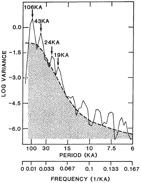
Figure 1 Power spectrum of a composite δ¹⁸O record using deep-sea cores RC11-120 and E49-18. This figure is based on the work of Hays et al. (1976), as presented by Imbrie and Imbrie (1986). Reprinted by permission from Springer Nature Customer Service Centre GmbH: Springer Nature. Topics in Geophysical Fluid Dynamics: Atmospheric Dynamics, Dynamo Theory, and Climate Dynamics by Ghil and Childress (1987), © 1987 by Springer Science+Business Media New York. All rights reserved. 1987.

The work of Hays et al. (1976) and of the subsequent CLIMAP and SPECMAP projects resulted in a much more detailed spatiotemporal mapping of the Quaternary and extended the belief in the pacemaking role of orbital variations into the more remote past. The spectral peaks near 20 and 40 kyr have been widely interpreted within the geological community as evidence for a linear response of the climate system to the orbital forcing (Imbrie and Imbrie, 1986). A third spectral peak at 100 kyr was, however, the most pronounced but much more difficult to reconcile with the orbital theory of Quaternary glaciations. Since no sufficiently pronounced counterpart can be found in the spectra of the seasonal insolation forcing, Hays et al. (1976) hypothesized a nonlinear response of the climate system in order to explain this dominant periodicity of the Late Pleistocene glacial–interglacial cycles. At the same time, the advent of higher-resolution marine cores and especially ice cores from both Greenland and Antarctica, led to the discovery of Heinrich events (Heinrich, 1988), Dansgaard–Oeschger (D-O) events (e.g., Dansgaard et al., 1993), and Bond cycles (Bond et al., 1997), which were hard to explain by orbital forcing given their shorter timescales.

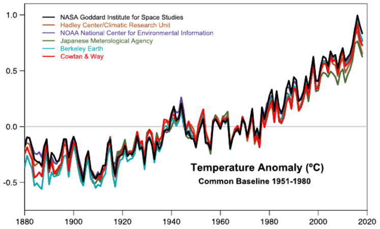
Figure 2 Comparison of six analyses of the annually and globally averaged surface temperature anomalies through 2018. The abscissa is time in years, and the ordinate is temperature anomalies in ^∘C with respect to a 30-year climatological average for 1951–1980. NASA stands for the National Aeronautics and Space Administration; NOAA stands for the National Oceanic and Atmospheric Administration. Reprinted by permission from John Wiley & Sons Inc.: American Geophysical Union. Journal of Geophysical Research: Atmospheres. Improvements in the GISTEMP Uncertainty Model. Lenssen et al. (2019), © 2019. American Geophysical Union. All Rights Reserved. 2019.

In fact, interest in past climates was heightened not only by these striking observational discoveries but also by the growing concerns about humanity's impact on the climate (SMIC, 1971; National Research Council, 1975). Given the declining temperatures between the 1940s and 1970s, on the one hand, as shown in Fig. 2 (see also Ghil and Vautard, 1991, Fig. 3), and the substantial advances in the description of the Quaternary glaciations, on the other hand, it is clear that interest was mainly on the planet's falling into another ice age (e.g., National Research Council, 1975).

As a result of the twofold stimulation provided by data about past glaciations and concern about future ones, a number of researchers in the early-to-mid 1970s worked on energy balance models (EBMs) of climate with multiple stable steady states (Held and Suarez, 1974; North, 1975; Ghil, 1976). Two such stable “equilibria” corresponded to the present climate and to a “deep-freeze”, as it was called at the time, i.e., to a totally ice-covered Earth. At the time there was some disbelief about this second climate, as its calculated temperatures were much lower than those associated with the Quaternary glaciations and incompatible with paleoclimatic evidence available in the 1970s.

New geochemical evidence, however, led in the early 1990s to the discovery of a “snowball” or, at least, “slushball” Earth prior to the emergence of multicellular life, sometime before 650 Myr b2k (Hoffman et al., 1998). It thus turned out that this climate state – predicted by several EBMs and confirmed by a general circulation model (GCM) with much higher spatial resolution (Wetherald and Manabe, 1975) – had actually occurred and is now being modeled in much greater detail (Pierrehumbert, 2004; Ghil and Lucarini, 2020).

On the other hand, it also became clear that these early models, whose only stable solutions were stationary, could not reproduce the wealth of variability that the proxy records were describing very well, not even in the presence of stochastic forcing (e.g., Ghil, 1994). Certain theoretical paleoclimatologists therefore turned to coupling a “climate” equation, with temperature as its only dependent variable, with an ice sheet equation (Källén et al., 1979; Ghil and Le Treut, 1981) or a carbon dioxide equation (Saltzman et al., 1981; Saltzman and Maasch, 1988). These coupled climate models, albeit highly idealized, did produce oscillatory solutions that captured some of the features of the Quaternary glaciation cycles as known at that time. For instance, the models of Ghil and associates (Källén et al., 1979; Ghil and Le Treut, 1981) captured the phase differences between peak ice sheet extent and minimum temperatures in the North Atlantic suggested by Ruddiman and McIntyre (1981), while the work of Saltzman and associates (e.g., Saltzman and Maasch, 1988) captured the asymmetry of the glaciation cycles with their more rapid “terminations” (Broecker and Van Donk, 1970).

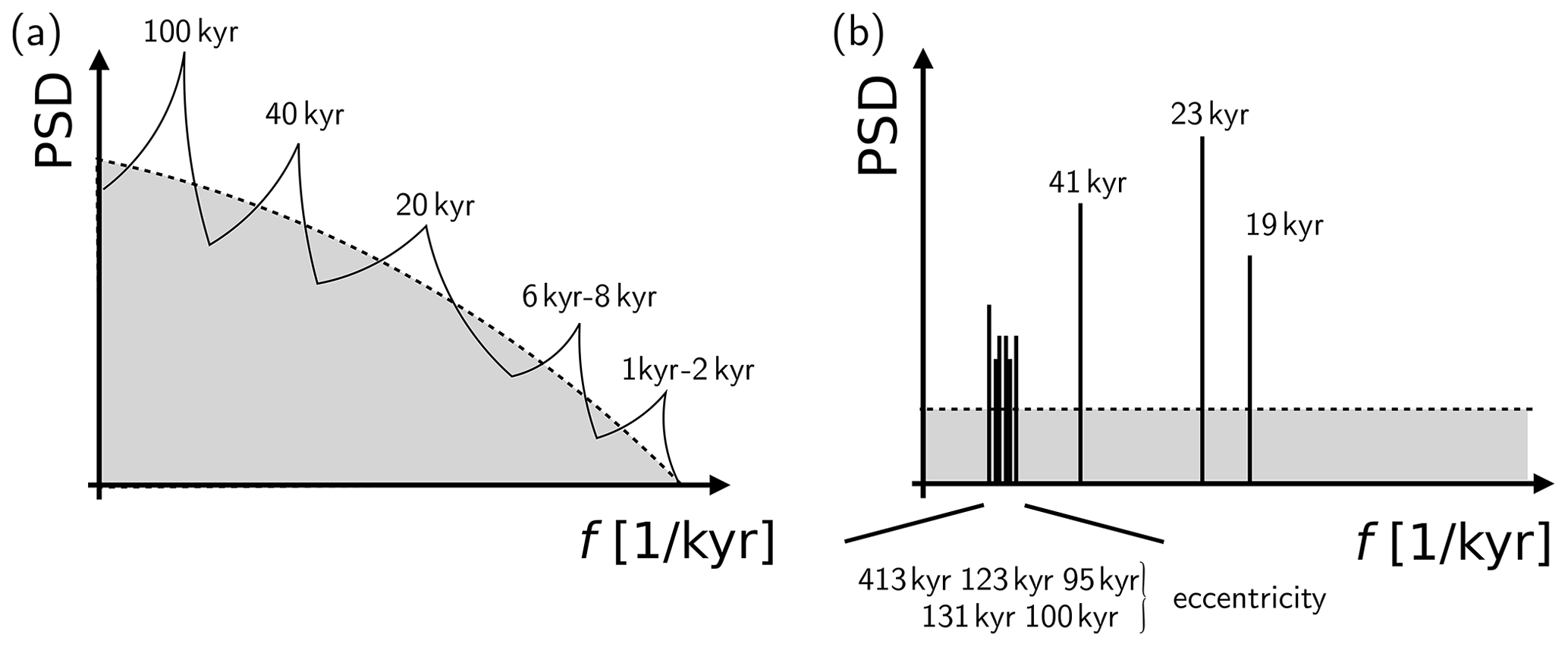
Figure 3 The theoretical quandary of modeling the Quaternary glaciation cycles, illustrated here by schematic diagrams of the composite power spectral densities (PSD) of (a) the paleo-records and (b) the orbital forcing. In panel (a), the dominant peak for the Late Pleistocene is near 100 kyr, while in panel (b) eccentricity forcing is distributed over several spectral lines. The peaks at 6–8 and 1–2 kyr in panel (a) correspond to Bond cycles (Bond et al., 1992, 1993) and to the mean recurrence of D-O events, and they lack a match in the forcing lines of panel (b).

The stable self-sustained oscillations of these coupled models, however, were totally independent of any orbital or other time-dependent forcing, i.e., the solar input to their radiative budget was constant in time. Hence, they could not capture the wealth of spectral features, with their orbital and other peaks, of the paleo-records available by the 1980s. The basic quandary of the Quaternary glaciation cycles – at least from the point of view of theoretical climate dynamics (Ghil and Childress, 1987, Part IV) – is formulated in Fig. 3 below; see also Ghil (1994): How does the quasi-periodic orbital forcing, with its relatively narrow spectral peaks, act on the climate's internal variability to produce a response that is characterized by significant spectral peaks superimposed on a broad continuous background? In addition, how does the climate's spectral peak at 100 kyr arise given its absence in the power spectrum of the forcing?

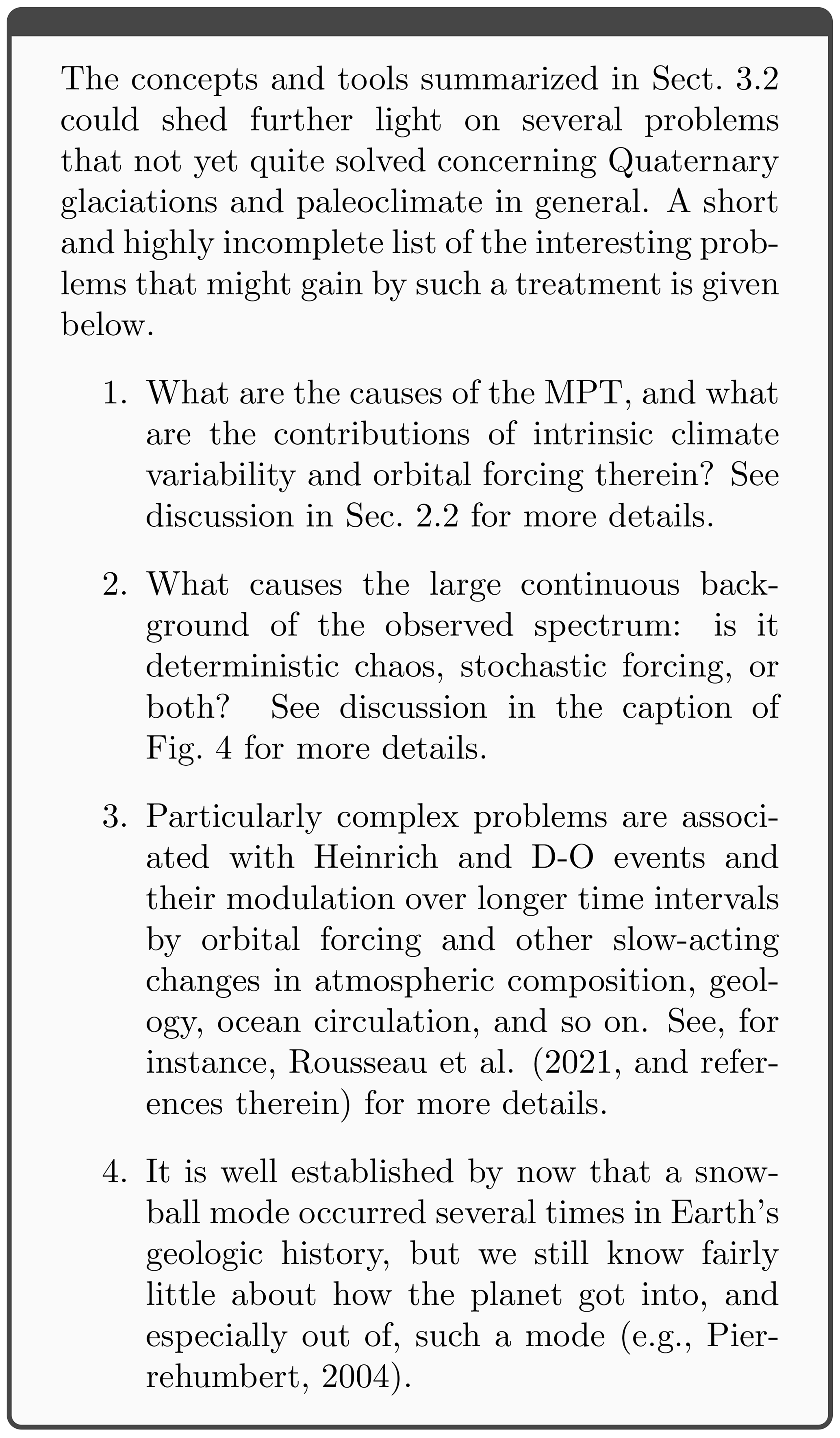
In this paper, we try to show a path toward resolving the four fundamental questions listed in Box 1. In the next section, we summarize existing results on how the climate system's intrinsic variability arises on Quaternary timescales and on how this variability is modified by the time-dependent orbital forcing, which was added to the previously autonomous climate models as the next step in paleoclimate modeling evolution; see, for instance, Le Treut and Ghil (1983) and Le Treut et al. (1988) vs. Ghil and Le Treut (1981). In Sect. 3, we outline a more general framework for the study of such mechanisms, as given by the theory of non-autonomous and random dynamical systems (NDSs and RDSs), and sketch an application of this theory to other climate problems. An application to the problem at hand is proposed in Sect. 4 and conclusions follow in Sect. 5.

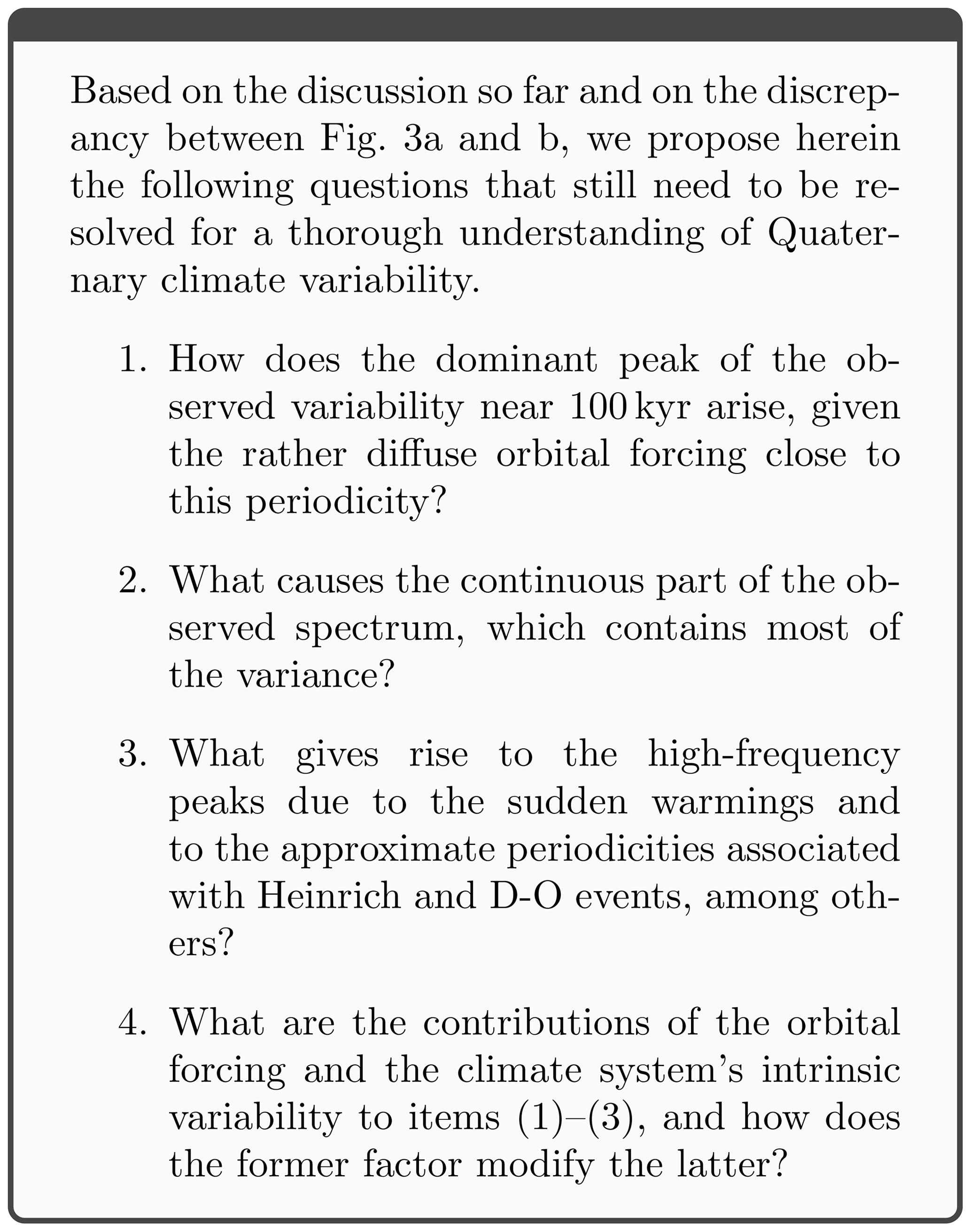
Box 1 Fundamental questions regarding the Quaternary glacial–interglacial cycles.

2 Self-sustained climate oscillators

2.1 A simple mechanism for climate oscillations

We follow Ghil (1994) in sketching the simplest physical mechanism for a self-sustained climate oscillation at fixed insolation forcing. Consider the Källén et al. (1979, hereafter KCG) oscillator, to the best of our knowledge the first such self-sustained climate oscillator. The model itself was built from the ground up, coupling a scalar version of the Ghil (1976) energy balance model (EBM) with a simplified, scalar version of the Weertman (1964, 1976) ice sheet model (ISM). The model's details and further analyses of its ingredients and variants can be found in several references (e.g., Crafoord and Källén, 1978; Ghil and Tavantzis, 1983; Ghil, 1984; Bódai et al., 2015).

The basic workings of this climate oscillator can be represented by two coupled ordinary differential equations (ODEs), written symbolically as follows:

$$\begin{array}{}\text{(1a)}& {\displaystyle }\dot{T}\simeq -V,\text{(1b)}& {\displaystyle }\dot{V}\simeq T.\end{array}$$

Here T stands for global temperature and V for global ice volume, while Eq. (1a) is an EBM and Eq. (1b) is an ice sheet model (ISM). The “≃” symbol stands for a binary relation of rough proportionality and is intended to neglect the details of the equation's right-hand side (RHS), including its nonlinearities. The EBM represents the well-known ice–albedo feedback used by both Budyko (1969) and Sellers (1969), while the ISM relies on the precipitation–temperature feedback postulated by KCG and used also by Ghil and Le Treut (1981), who coined the term.

The latter feedback can be better understood by writing the following equations:

$$\begin{array}{}\text{(2a)}& {\displaystyle }\dot{V}\simeq p,\text{(2b)}& {\displaystyle }p\simeq p_{\text{ac}}-p_{\text{ab}},\text{(2c)}& {\displaystyle }{p}_{\text{ac}}\simeq T.\end{array}$$

Here p is net precipitation on the single ice sheet of the globally integrated model, given by the difference in Eq. (2b) between the accumulation p_ac and the ablation p_ab (KCG).

As first observed by George C. Simpson – the meteorologist of Robert F. Scott's Terra Nova expedition to Antarctica in 1910–1912 and later the longest-serving Director of the U.K. Meteorological Office – warmer winters have more snow, and hence, at least in central Antarctica, the increase of p_ac with T exceeds the more obvious increase of p_ab with T. Hence, p≃T, and we have derived therewith Eq. (1b), i.e., $V\simeq p\simeq T$. For more recent studies of the precipitation–temperature feedback, see Tziperman and Gildor (2002).

More generally, the presence of feedbacks of opposite sign in a system of two linear coupled ODEs,

$$\dot{x}=y,\dot{y}=-x,$$

leads to an oscillation, with the solution given by two trigonometric functions in quadrature with each other, x(t)=sin (t), $y\left(t\right)=\cos \left(t\right)=\sin (t+\mathit{\pi }/\mathrm{2})$, and the trajectory describing a circle in the (x,y) phase plane, $x^{\mathrm{2}}\left(t\right)+y^{\mathrm{2}}\left(t\right)=\mathrm{1}$. In a nonlinear system, however – like the full KCG model or any other climate oscillator mentioned so far – the possibility of an oscillation, as indicated by the system (1), is actually realized in the explicit, full set of equations only for certain parameter values and not for others.

This can be understood by considering the so-called normal form of a Hopf bifurcation, which leads from a stable steady state, called a fixed point in dynamical systems theory, to a stable oscillatory solution, called a limit cycle. The easiest way to see this transition is by writing the normal form in polar coordinates, as in Arnold (1988) and in Ghil and Childress (1987, Sect. 12.2), namely,

$$\begin{array}{}\text{(3)}& \dot{z}=(\mathit{\mu }+\mathit{ı}\mathit{\omega })z+c\left(z\stackrel{\mathrm{‾}}{z}\right)z.\end{array}$$

Here $z=x+\mathit{ı}y$ is complex, where $\mathit{ı}=\sqrt{-\mathrm{1}}$ is the imaginary unit, while μ is a real bifurcation parameter, and c,ω are real and nonzero. Note that the KCG model per se is not in the normal form above, and we will discuss its bifurcation parameter μ_∗ in the next subsection.

Figure 4 Supercritical Hopf bifurcation. (a) Vector field $\dot{z}\left(z\right)$ of Eq. (3) for the parameter values $\mathit{\mu }=-\mathrm{1}$ and $c=-\mathrm{1}$; $z=x+\mathit{ı}y$. In this case, the origin constitutes the only stable fixed point, and all trajectories will spiral into this point, as illustrated by the single brown trajectory. (b) Vector field $\dot{z}\left(z\right)$ and three trajectories for μ=1. In this case, the origin is an unstable fixed point, while the limit cycle with radius ${\mathit{\rho }}_{*}^{\mathrm{1}/\mathrm{2}}=\mathrm{1}$ constitutes the only stable solution. Trajectories that start inside this limit cycle, with $\mathit{\rho }\left(t_{\mathrm{0}}\right)<{\mathit{\rho }}_{*}$, tend to it by spiraling out – as illustrated by the magenta trajectory – while trajectories that start outside the limit cycle, with $\mathit{\rho }\left(t_{\mathrm{0}}\right)>{\mathit{\rho }}_{*}$, approach it by spiraling inward, as illustrated by the gray trajectory. (c) Dependence of the stable solution of Eq. (3) on the parameter μ, for $c=-\mathrm{1}$. For μ≤0, the single stable solution is the fixed point located at the origin, ρ≡0. For μ>0, the stable solution is the limit cycle given by ρ=μ.

A very natural transformation of variables,

$$\begin{array}{}\text{(4)}& \mathit{\rho }=z\stackrel{\mathrm{‾}}{z}>\mathrm{0},z={\mathit{\rho }}^{\mathrm{1}/\mathrm{2}}\exp \left(\mathit{ı}\mathit{\theta }\right),\end{array}$$

leads from the complex ODE (3) to the system of two real and decoupled ODEs,

$$\begin{array}{}\text{(5a)}& {\displaystyle }\dot{\mathit{\rho }}=\mathrm{2}\mathit{\rho }(\mathit{\mu }+c\mathit{\rho }),\text{(5b)}& {\displaystyle }\dot{\mathit{\theta }}=\mathit{\omega }.\end{array}$$

Equation (5b) simply provides an angular rotation around the origin $\mathit{\rho }=\mathrm{0}=x=y$, since the complex exponential in Eq. (4) is periodic with period 2π. Equation (5a) is quadratic in ρ, and thus it can have two real roots, $\mathit{\rho }={\mathit{\rho }}_{\mathrm{0}}=\mathrm{0}$ and $\mathit{\rho }={\mathit{\rho }}_{\ast }=-\mathit{\mu }/c$. But ρ has to be positive, and thus in the case in which c<0, the only possible solution for μ<0 is the origin, and it is stable since ρ(μ+cρ) is negative for ρ>0 in this case; hence, ρ has to be monotonically decreasing, i.e., all the solutions of Eq. (5) spiral into the origin. The Hopf bifurcation from this stable steady state to a periodic solution, i.e., a limit cycle with radius ${\mathit{\rho }}^{\mathrm{1}/\mathrm{2}}={\mathit{\rho }}_{\ast }^{\mathrm{1}/\mathrm{2}}$, occurs as μ crosses 0. Since now $\mathit{\rho }(\mathit{\mu }+c\mathit{\rho })>\mathrm{0}$ for $\mathrm{0}<\mathit{\rho }<{\mathit{\rho }}_{\ast }$ and $\mathit{\rho }(\mathit{\mu }+c\mathit{\rho })<\mathrm{0}$ for $\mathit{\rho }>{\mathit{\rho }}_{\ast }$, the limit cycle is stable and trajectories spiral out from inside this cycle and into it from outside; see Fig. 4 for the so-called supercritical (or soft) Hopf bifurcation case with c<0.

2.2 Intrinsic climate oscillations and the mid-Pleistocene transition (MPT)

In this subsection, we present an argument for the role of intrinsic oscillations in the mid-Pleistocene transition (MPT). The first point to be made is that while orbital forcing clearly plays a major role in the power spectrum of the Quaternary's climatic variability, it cannot be, in and of itself, the cause of the MPT. Indeed, changes in the solar system's orbital periodicities only occur on much longer timescales than the entire Quaternary's duration (Varadi et al., 2003; Laskar et al., 2004a). Our argument continues with a further analysis of the Hopf bifurcation presented in the previous subsection. Such an analysis was carried out for the KCG model by Ghil and Tavantzis (1983).

Physically speaking, the presence or absence of the regular, purely periodic oscillations obtained by KCG and illustrated in Ghil and Childress (1987, Fig. 12.6) depends on whether c≷0 in Eq. (5a). The KCG model's bifurcation parameter is ${\mathit{\mu }}_{\ast }=c_T/c_L$, where c_T is the heat capacity in its EBM, while c_L is the “mass capacity” in its ISM (Ghil and Tavantzis, 1983). Large μ_∗ corresponds physically to a very small, possibly pre-Pleistocene ice cap (Ghil, 1984; Saltzman and Sutera, 1987). At these values of μ_∗, the KCG model's nullclines and fixed points – the latter being given by the intersection of the former – are very different from those that are obtained for Quaternary-sized ice sheets, for which c_L is comparable in value to c_T; see Ghil and Tavantzis (1983, Figs. 3–5). As μ_∗ decreases to O(1), i.e., as we proceed from very small to more substantial ice sheets, the fixed point transfers its stability to a branch of periodic solutions via a subcritical Hopf bifurcation (Källén et al., 1979; Ghil and Tavantzis, 1983); see also Ghil and Childress (1987, Figs. 12.8 and 12.9).

To clarify the simple physical concepts that underlie subcritical and supercritical Hop bifurcations, let us consider a purely mechanical oscillator with mass m, a spring kx, and a dashpot $\mathit{\alpha }\dot{x}$ (Landau and Lifshitz, 1960; Jordan and Smith, 1987),

$$\begin{array}{}\text{(6)}& m\ddot{x}=-\mathit{\alpha }\left(x\right)\dot{x}-k\left(x\right)x.\end{array}$$

If k = const. and α = const., we have the simplest, linear setup, but we will be interested in the nonlinear cases here. Normalizing by the mass m and not changing notation otherwise, by rearranging terms and adding a periodic forcing we get the following equation:

$$\begin{array}{}\text{(7)}& \ddot{x}+\mathit{\alpha }\left(x\right)\dot{x}+k\left(x\right)x=F\cos \left(\mathit{\omega }t\right).\end{array}$$

Two classical nonlinear cases are those of the Duffing (1918) equation, in which k(x)=x² and α = const., and of the Van der Pol (1926) equation, in which k = const. and $\mathit{\alpha }\left(x\right)=\mathit{\nu }(x^{\mathrm{2}}-\mathrm{1})$. The fully nonlinear case in which both the spring and the damping are nonlinear, with k(x)=x² and $\mathit{\alpha }\left(x\right)=\mathit{\nu }(x^{\mathrm{2}}-\mathrm{1})$, is known as the Van der Pol–Duffing oscillator (e.g., Jackson, 1991; Pierini et al., 2018). Note that all three types of nonlinear oscillators can exhibit chaotic behavior even in the presence of simple periodic forcing (e.g., Guckenheimer and Holmes, 1983; Pierini et al., 2018, and references therein). The idea of using such simple, classical oscillators in modeling Quaternary glaciation cycles goes back to Saltzman et al. (1981).

Jordan and Smith (1987, Sect. 5.6) specifically discuss the case of a soft and a hard spring for a generalized Duffing equation, with $k\left(x\right)=k_{\mathrm{0}}+\mathit{ϵ}h\left(x\right)$, where $\mathrm{0}<\left|\mathit{ϵ}\right|\ll \mathrm{1}$, $h(-x)=h\left(x\right)$, and $h^{\prime \prime }>\mathrm{0}$. A spring is soft if it is sublinear, ϵ<0, and hard if it is superlinear, ϵ>0; see their Eq. (5.37) and Fig. 5.4a, b, with h(x)=x².

The supercritical Hopf bifurcation in the absence of forcing is analogous to the nonlinear response of a soft, sublinear spring to periodic forcing in which the oscillations in the position x of the mass m increase gradually in amplitude as the spring constant k₀ increases past a critical value k_∗, while the subcritical case is analogous to the response of a hard, superlinear spring, for which the oscillations in x jump suddenly from zero amplitude to a finite amplitude as the spring constant k₀ crosses the value k_∗. Please compare the behavior of supercritical and subcritical Hopf bifurcations in Ghil and Childress (1987, Sect. 12.2 and Figs. 12.7–12.9) and see Jordan and Smith (1987, Fig. 5.7) for the change in the nonlinear response of a Duffing oscillator as its spring changes from soft, with ϵ<0, to hard, with ϵ>0.

There is a clear-cut analogy with the mid-Pleistocene transition, occurring at roughly 0.8 Ma b2k, at which small-amplitude climate variability with a dominant periodicity near 40 kyr becomes larger, dominated by a periodicity that is close to 100 kyr, as well as being more irregular (e.g., Huybers, 2009; Quinn et al., 2018; Rousseau et al., 2020). A fair number of distinct dynamical theories for this transition have been formulated (e.g., Maasch and Saltzman, 1990; Ghil, 1994; Crucifix, 2012; Ashwin and Ditlevsen, 2015; Daruka and Ditlevsen, 2016; Omta et al., 2016; Ditlevsen and Ashwin, 2018). A rather obvious one is that a Hopf bifurcation occurs at that point, which leads to a more vigorous response to the multi-periodic orbital forcing; thus, the latter does not need to change in the least in order to explain the observed phenomena. In Saltzman and Sutera (1987), there is only a comment on the likely role of a Hopf bifurcation in the transition, but their Fig. 3 suggests that in their model such a bifurcation would have to be of the supercritical type and lead to a fairly gradual transition.

In contrast, the subcritical Hopf bifurcation of the KCG and Ghil and Le Treut (1981) oscillators would have to lead to a more abrupt transition, as suggested by Ghil (1984). Later, Crucifix (2012) showed that the models by Saltzman and Maasch (1990, 1991) exhibit MPT-like behavior via supercritical or subcritical Hopf bifurcations, depending on the parameter values. The existing δ¹⁸O and δ¹³C records might or might not have sufficient resolution back in time up to 1.2 Ma to settle this question about the abruptness of the transition. In case some of them do, an objective test of suddenness – as proposed by Bagniewski et al. (2021) for the high-resolution NGRIP record (North Greenland Ice Core Project members, 2004) – will have to be applied to such records.

3 Time-dependent forcing, NDSs, and RDSs

3.1 Orbital forcing of a climate oscillator

We start this section by describing some fairly simple ways in which the orbital forcing might have modified intrinsic climate variability, thus helping to solve the mismatch between Fig. 3a and b in Sect. 1. To explore this possibility, Le Treut and Ghil (1983) used somewhat simplified insolation forcing based on the calculations of Berger (1978) and applied it to a slightly modified version of the Ghil and Le Treut (1981) oscillator. These authors found that, as expected for a nonlinear oscillator, its internal frequency f₀ is affected strongly by the forcing ones, $\mathit{\{}{f}_{\mathrm{1}},\mathrm{\dots },f_{\mathrm{5}}\mathit{\}}$, resulting in both nonlinear resonance and combination tones (Landau and Lifshitz, 1960).

Depending on parameter values, the periodicity $P_{\mathrm{0}}=\mathrm{1}/f_{\mathrm{0}}$ of the Ghil and Le Treut (1981) oscillator is P₀≃6–7 kyr. The lines in the simplified insolation spectrum used by Le Treut and Ghil (1983) had the following periodicities: P₁=19 kyr, P₂=23 kyr, P₃=41 kyr, P₄=100 kyr, and P₅=400 kyr. These periodicities correspond to the two precessional ones, the obliquity one, and the two eccentricity ones. The actual celestial-mechanics calculations that Berger (1978) based his insolation calculations on have been substantially updated since (e.g., Varadi et al., 2003; Fienga et al., 2015). However, these advances have not modified the spectrum of the planetary-orbit solutions over the 2.6 Myr of the Quaternary very much, which is a rather short interval in celestial-mechanics terms.

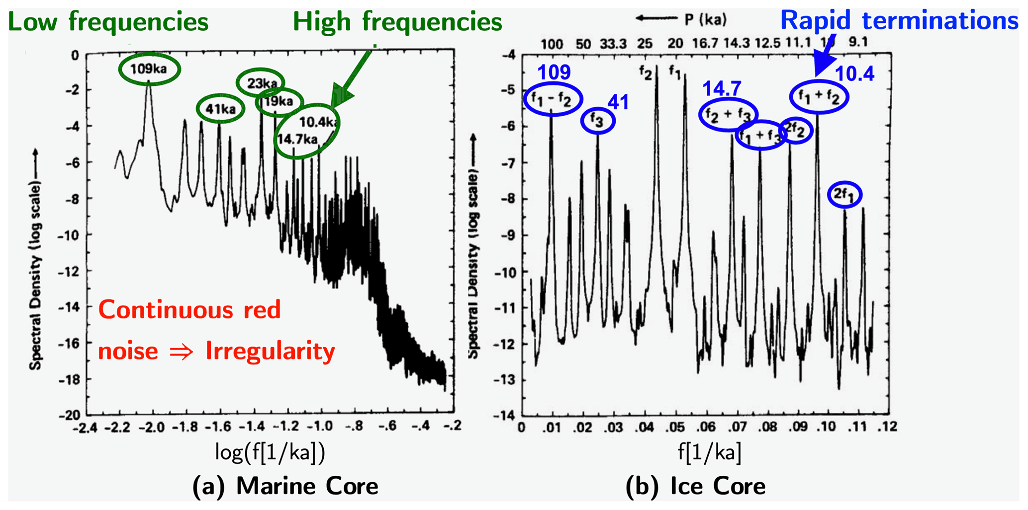
Figure 5 Power spectra of simulated (a) deep-sea and (b) ice core records for the forced climate oscillator of Le Treut et al. (1988) with idealized orbital forcing. Panel (a) is in log–log coordinates and clearly shows a dominant peak at 109 kyr and a very large amount of variance in the continuous spectrum, which has a roughly −2 power law slope. The orbital peaks at P₁=19 kyr, P₂=23 kyr and P₃=41 kyr are also present, along with peaks at 14.7 and 10.4 kyr, which correspond to the sum tones f₂+f₃ and f₁+f₂, respectively. Panel (b) is in log–linear coordinates and shows additional harmonics and sum tones, as well as the difference tone f₁−f₂, which corresponds to the dominant peak at 109 kyr. Inside the figure, the notation ka instead of kyr has been kept unchanged from the original publication. Adapted by permission from John Wiley & Sons Inc.: American Geophysical Union. Journal of Geophysical Research: Atmospheres. Isotopic Modeling of Climatic Oscillations: Implications for a Comparative Study of Marine and Ice Core Records by Le Treut et al. (1988), © 1988 by the American Geophysical Union. 1988.

The results of the Le Treut and Ghil (1983) model on the evolution of the primary climate variables T and V were converted to δ¹⁸O values in simulated isotopic records of marine sediment and ice cores by Le Treut et al. (1988); the spectra of the latter are plotted in Fig. 5. The values on the abscissa of Fig. 5a are values of the logarithm of frequency, while those in Fig. 5b are values of the frequency itself; the values on the ordinate of both panels are powers of 10. One refers to such figures as being in (a) log–log coordinates vs. (b) log–linear coordinates for short.

Aside from the spectral features noted in the figure caption and discussed in greater detail by Ghil (1994), it is important to realize (i) that the large continuous background in Fig. 5a is purely of deterministically chaotic origin since there is no stochastic element whatsoever in the Le Treut and Ghil (1983) model or in its forcing and (ii) that the dominant peak at 109 kyr is not directly forced by the $f_{\mathrm{4}}=\mathrm{1}/\mathrm{100}$ kyr⁻¹ eccentricity line but rather it is due to the difference tone between the two precessional frequencies, f₁ and f₂. Finally, it is the nonlinear, broad resonance of the model's f₀ frequency with the quasi-periodic forcing that produces the bump in the spectrum of Fig. 5a to the right of the orbital frequencies.

In returning to the “fundamental question no. 2” in Box 1, one must recall that on the paleoclimatic timescales of interest – apart from deterministic chaos à la Lorenz (1963), as obtained by Le Treut and Ghil (1983) and Le Treut et al. (1988) and shown here in Fig. 5a – stochastic contributions à la Hasselmann (1976) to the continuous part of the spectrum must also play an important role. In fact, RDS theory, as outlined in the next subsection, provides an excellent framework for a “grand unification” of these two complementary points of view (Ghil, 2014, 2019). In the paleoclimatic context, Ditlevsen et al. (2020) have suggested that, aside from red noise processes, dating uncertainties in the proxy records from which the spectra are derived may contribute, in all likelihood, to this background; see also Boers et al. (2017a, b). In this context, Verbitsky and Crucifix (2020) also provide a simple theory that addresses scaling properties in the glacial cycles and their spectra, based on the so-called Buckingham π-theorem (e.g., Barenblatt, 1996).

3.2 Basic facts of NDS and RDS life

The highly preliminary results summarized in Sect. 3.1 encourage us to pursue the effects of the orbital forcing on intrinsic climatic variability in a more systematic way, effects that may have contributed to generate the rich paleoclimate spectrum on Quaternary and longer timescales (e.g., Westerhold et al., 2020). In fact, several research groups in the climate sciences have carried out during the past 2 decades an important extension of the dynamical systems and model hierarchy framework presented by Ghil and Childress (1987) and by Ghil (2001), from deterministically autonomous to non-autonomous and random dynamical systems (NDSs and RDSs, e.g., Ghil et al., 2008; Chekroun et al., 2011; Bódai and Tél, 2012).

On the road to including deterministically time-dependent and random effects, one needs to realize first that the climate system – as well as any of its subsystems on any timescale – is not closed: it exchanges energy, mass, and momentum with its surroundings, whether this pertains to other subsystems or the interplanetary space and the solid earth. The typical applications of dynamical systems theory to climate variability until not so long ago have only taken into account exchanges that are constant in time, thus keeping the model – whether governed by ordinary, partial, or other differential equations – autonomous; i.e., the models had coefficients and forcings that were constant in time.

Alternatively, the external forcing or the parameters were assumed to change either much more slowly than a model's internal variability, meaning that the changes could be assumed to be quasi-adiabatic, or much faster, meaning that they could be approximated by stochastic processes. Some of these issues are covered in much greater detail by Ghil and Lucarini (2020, Sect. III.G). The key concepts and tools of NDSs and RDSs go beyond such approaches that rely in an essential way on a scale separation between the characteristic times of the forcing and the internal variability of a given system; such a separation is rarely if ever actually present in the climate sciences.

The presentation of the key NDS and RDS concepts and tools in this subsection is aimed at as large a readership as possible and follows Ghil (2014). Slightly more in-depth but still fairly expository presentations can be found in Crauel and Kloeden (2015) and in Caraballo and Han (2017). Readers who are less interested in this mathematical framework – which allows a truly thorough understanding of the way that orbital forcing acts on intrinsic climate variability on Quaternary timescales – may skip at a first reading the remainder of this section and continue with Sect. 4.

3.2.1 Autonomous and non-autonomous systems

Succinctly, one can write an autonomous system as

$$\begin{array}{}\text{(8)}& \dot{\mathit{X}}=\mathit{F}(\mathit{X};\mathit{\mu }),\end{array}$$

where X stands for any state vector or climate field. While F is a smooth function of X and of the parameter μ, it does not depend explicitly on time. This autonomous character of Eq. (8) greatly facilitates the analysis of its solutions' properties.

For instance, two distinct trajectories, X₁(t) and X₂(t), of a well-behaved, smooth autonomous system cannot intersect – i.e., they cannot pass through the same point in phase space – because of the uniqueness of solutions. This property helps one draw the phase portrait of an autonomous system, as does the fact that we only need to consider the behavior of solutions X(t) as time t tends to +∞. The sets of points so obtained are (possibly multiple) equilibria, periodic and quasi-periodic solutions, and chaotic sets. In the language of dynamical systems theory, these are called, respectively: fixed points, limit cycles, tori, and strange attractors.

We know only too well, however, that the seasonal cycle plays a key role in climate variability on interannual timescales, while orbital forcing is crucial on the Quaternary timescales of many millennia. In addition, more recently it has become obvious that anthropogenic forcing is of utmost importance on the interdecadal timescales between these two extremes.

How can one take into account these types of time-dependent forcings and analyze the non-autonomous systems that they lead us to formulate? One succinctly writes such a system as follows:

$$\begin{array}{}\text{(9)}& \dot{\mathit{X}}=\mathit{F}(\mathit{X},t;\mathit{\mu }).\end{array}$$

In Eq. (9), the dependence of F on t may be periodic, $\mathit{F}(\mathit{X},t+P)=\mathit{F}(\mathit{X},t)$, as in various El Niño–Southern Oscillation (ENSO) models, where the period P=12 months, or monotonic, $\left|\mathit{F}\right|(\mathit{X},t+\mathit{\tau })\ge \left|\mathit{F}\right|(\mathit{X},t)$, as it is when studying scenarios of anthropogenic climate forcing. An even more general situation includes time dependence in one or more parameters $\mathit{\{}{\mathit{\mu }}_{\mathrm{1}},\mathrm{\dots },{\mathit{\mu }}_p\mathit{\}}$.

To illustrate the fundamental distinction between an autonomous system like Eq. (8) and a non-autonomous one like Eq. (9), consider the simple scalar version of these two equations:

$$\begin{array}{}\text{(10a)}& \dot{X}=-\mathit{\beta }X,\end{array}$$

and

$$\begin{array}{}\text{(10b)}& \dot{X}=-\mathit{\beta }X+\mathit{\gamma }t,\end{array}$$

respectively. We assume that both systems are dissipative, i.e., β>0, and that the forcing is monotonically increasing, γ≥0, as would be the case for anthropogenic forcing in the industrial era. Lorenz (1963) pointed out the key role of dissipativity in giving rise to strange but attracting solution behavior, while Ghil and Childress (1987) emphasized its importance and pervasive character in climate dynamics. Clearly the only attractor for the solutions of Eq. (10a), given any initial point X(0)=X₀, is the stable fixed point $X_{\ast }=\mathrm{0}$, attained as $t\to +\mathrm{\infty }$.

In the case of Eq. (10b), however, this forward-in-time approach yields blow-up from $t\to +\mathrm{\infty }$ for any initial point. To make sense of what happens in the case of time-dependent forcing, one instead introduces the pullback approach, in which solutions are allowed to still depend on the time t at which we observe them but also on a time s from which the solution is started, with X(s)=X₀ and s≪t. With this little change of approach, one can easily verify that

$$\begin{array}{}\text{(11)}& \left|X\right(s,t;X_{\mathrm{0}})-{\mathcal{A}}_t|\to \mathrm{0}\text{as}s\to -\mathrm{\infty },\end{array}$$

for all t and X₀, where ${\mathcal{A}}_t=(\mathit{\gamma }/\mathit{\beta })(t-\mathrm{1}/\mathit{\beta })$. We obtain therewith, in this pullback sense, the intuitively obvious result that the solutions, if we start them far enough in the past, all approach the family of attracting sets 𝒜_t; this family follows the forcing γt, and it thus has a linear growth in time t. Hence, the fixed point X_∗ of Eq. (10b) is in fact a moving target and it is given by $X_{\ast }=\mathit{\gamma }t/\mathit{\beta }$. Due to the system's inertia, the set 𝒜_t that is approached by the trajectories lags this time-dependent fixed point by a constant offset of $\mathit{\gamma }/{\mathit{\beta }}^{\mathrm{2}}$.

3.2.2 Pullback attractor (PBA)

Formally, the indexed family of all pullback attracting sets 𝒜_t,

$$\begin{array}{}\text{(12)}& \textcolor{red}{}=\mathit{\{}{\mathcal{A}}_t{\mathit{\}}}_{t\in \mathbb{R}},\end{array}$$

is termed the pullback attractor (PBA) of an NDS if the following two conditions are fulfilled:

• i.

  each snapshot 𝒜_t is compact and the family of snapshots {𝒜(t)}_t∈ℝ is invariant with respect to the dynamics,

  $$\begin{array}{}\text{(13)}& \mathit{X}(t,s;{\mathit{X}}_{\mathrm{0}})\in {\mathcal{A}}_t\forall s\le t\mathrm{and}{\mathit{X}}_{\mathrm{0}}\in A_s,\end{array}$$

  and

• ii.

  the pullback attraction occurs for all times,

  $$\begin{array}{}\text{(14)}& \underset{s\to -\mathrm{\infty }}{lim}\left|\mathit{X}\right(t,s;{\mathit{X}}_{\mathrm{0}})-{\mathcal{A}}_t|=\mathrm{0}\forall t.\end{array}$$

To further improve the reader's intuition for PBAs, we provide a second illustrative example here. A system defined in polar coordinates by

$$\begin{array}{}\text{(15)}& \dot{\mathit{\rho }}=\mathit{\alpha }(\mathit{\mu }-\mathit{\rho }),\dot{\mathit{\varphi }}=\mathit{\omega },\end{array}$$

with $\mathit{\rho },\mathit{\mu }\in {\mathbb{R}}^{+}$, and $\mathit{\varphi }\in \mathbb{R}/\mathrm{2}\mathit{\pi }$ can easily be seen to exhibit a limit cycle in the (x,y) plane with $(x=\mathit{\rho }\cos \mathit{\varphi },y=\mathit{\rho }\sin \mathit{\varphi })$. An initial deviation of ρ from μ will decay exponentially, and the system converges to an oscillation of radius μ with the angular velocity ω. Here, we transform this autonomous dynamical system into a non-autonomous one by modulating the target radius μ with a sinusoidal forcing,

$$\begin{array}{}\text{(16)}& \mathit{\mu }\to \mathit{\mu }\left(t\right)={\mathit{\mu }}_{\mathrm{0}}+\mathit{\beta }\sin \left(\mathit{\nu }t\right),\end{array}$$

where the modulation is moderate to guarantee that ${\mathit{\mu }}_{\mathrm{0}}+\mathit{\beta }\sin \left(\mathit{\nu }t\right)>\mathrm{0}$ for all t.

Since the dynamics of the phase ϕ and of the radius ρ are decoupled, the corresponding equations can be solved and analyzed separately. While the temporal development of the phase is trivial, the pullback-invariant attracting set of the radius for the initial condition ρ(s)=ρ₀ is given by

$$\begin{array}{}\text{(17a)}& {\mathcal{A}}^{\left(\mathit{\rho }\right)}(t;{\mathit{\rho }}_{\mathrm{0}})=\underset{s\to -\mathrm{\infty }}{lim}\mathit{\rho }(t,s;{\mathit{\rho }}_{\mathrm{0}})=\mathit{\alpha }\mathit{\beta }\sin (\mathit{\nu }t+\mathit{\vartheta })+{\mathit{\mu }}_{\mathrm{0}},\end{array}$$

with

$$\begin{array}{}\text{(17b)}& \mathit{\vartheta }=\arctan (-\mathit{\nu }/\mathit{\alpha }),\end{array}$$

as shown in Appendix B. Note that in the limit $s\to -\mathrm{\infty }$, the dependence on the initial value ρ₀ vanishes and the attracting set ${\mathcal{A}}_t^{\left(\mathit{\rho }\right)}$ performs an oscillation of the same frequency as the forcing. It lags the phase of the time-dependent fixed point μ(t) by the constant ϑ, while its amplitude is amplified by the factor α. Since ρ is restricted to positive values, this solution requires αβ<μ₀.

The PBA with respect to the coordinate ρ is comprised of the family of all the sets ${\mathcal{A}}_t^{\left(\mathit{\rho }\right)}$ as defined in Eq. (18) and thus reads

$$\begin{array}{}\text{(18)}& \textcolor{red}{}=\mathit{\left\{}\mathit{\alpha }\mathit{\beta }\sin \right(\mathit{\nu }t+\mathit{\vartheta })+{\mathit{\mu }}_{\mathrm{0}}{\mathit{\}}}_{t\in \mathbb{R}}.\end{array}$$

Since the pullback limit for the phase ϕ does not exist, no constraints on it other than $\mathit{\varphi }\in [\mathrm{0},\mathrm{2}\mathit{\pi })$ are imposed by the dynamics. Hence, for the system (15) comprised of radius and phase, we find that the distance of any trajectory at time t – i.e. $\left(\mathit{\rho }(t;t_{\mathrm{0}},{\mathit{\rho }}_{\mathrm{0}}),\mathit{\varphi }(t;t_{\mathrm{0}},{\mathit{\varphi }}_{\mathrm{0}})\right)$ – to the set ${\mathcal{A}}_t=\mathit{\{}\left(\mathit{\alpha }\mathit{\beta }\sin (\mathit{\nu }t+\mathit{\vartheta })+{\mathit{\mu }}_{\mathrm{0}},\mathit{\phi }\right):\mathit{\phi }\in [\mathrm{0},\mathrm{2}\mathit{\pi }\left)\mathit{\right\}}$ tends to zero as we pullback the initial time t₀ to −∞. The pullback attracting sets 𝒜_t at time t are circles in the (x,y) plane with a radius that oscillates in time, and the system's PBA is given by the family of these circles

$$\begin{array}{}\text{(19)}& \textcolor{red}{}=\mathit{\{}\left(\mathit{\alpha }\mathit{\beta }\sin (\mathit{\nu }t+\mathit{\vartheta })+{\mathit{\mu }}_{\mathrm{0}},\mathit{\phi }\right):\mathit{\phi }\in [\mathrm{0},\mathrm{2}\mathit{\pi }){\mathit{\}}}_{t\in \mathbb{R}}.\end{array}$$

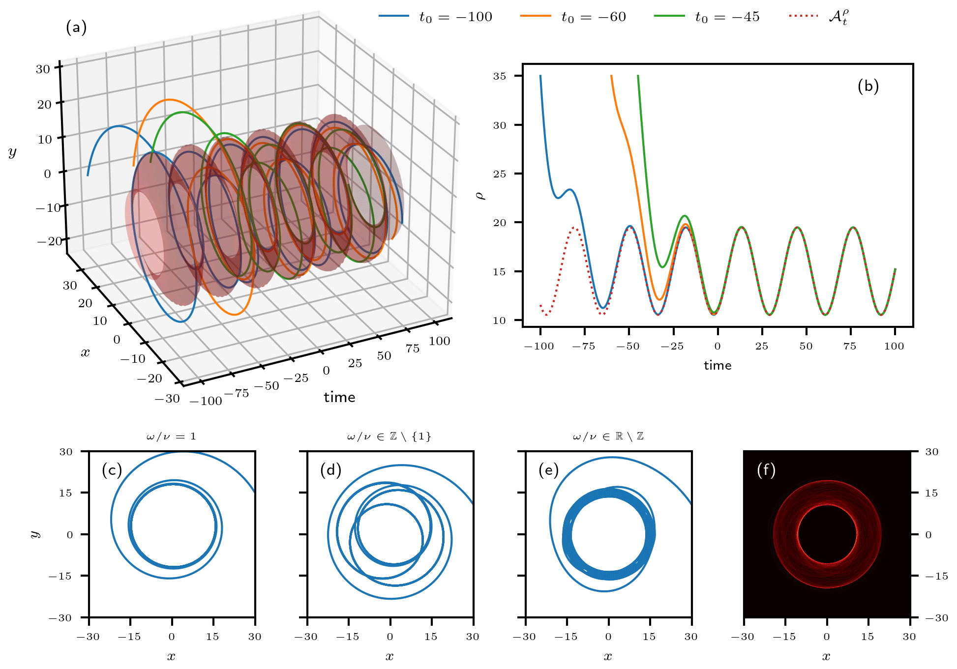
Figure 6 Trajectories and PBA of the system defined by Eqs. (15) and (16); in all the panels the parameter values are μ₀=15, α=10, ν=0.2, and ω=0.3, unless stated otherwise. (a) Trajectories (ρ(t),ϕ(t)) of the system starting from different times in the past in the 3-D space spanned by (x,y) and time t; the system's PBA lies on the red-shaded surface. (b) Temporal evolution of the radius (solid colors) of the three trajectories shown in (a) together with its PBA (dotted red). (c–e) Trajectories integrated from $t_{\mathrm{0}}=-\mathrm{100}$ to t_f=200 for $\mathit{\nu }=\mathrm{0.3},\mathrm{0.2},{\mathrm{0.5}}^{\mathrm{1}/\mathrm{2}}$ in panels (c), (d), and (e), respectively. The values are chosen such that the ratio between ν and ω is $\mathit{\omega }/\mathit{\nu }=\mathrm{1}$, $\mathit{\omega }/\mathit{\nu }\in \mathbb{Z}\backslash \mathit{\left\{}\mathrm{1}\mathit{\right\}}$ and $\mathit{\omega }/\mathit{\nu }\in \mathbb{R}\backslash \mathbb{Z}$ in panels (c) to (e). Correspondingly, in (c) the trajectory quickly converges to a circle, whose center is slightly shifted from the origin. In panel (d) a quasi-closed three-fold loop can be observed, since $\mathit{\omega }/\mathit{\nu }=\mathrm{3}/\mathrm{2}$. In panel (e) the trajectories will densely fill the annular disk defined in the video supplement statement. (f) Heat map of numerous trajectories projected onto the (x,y) plane. The trajectories start at random points in state space and are integrated from $t_{\mathrm{i}}=-\mathrm{200}$ to t_f=200. A video of the heat map filling up as more and more trajectories with different initial conditions are added is provided in the video supplement. The heat map shown here is a snapshot of the video taken at time t=0.20; see details in the video supplement.

Figure 6 shows trajectories of the system starting from different points in the past. In Fig. 6a, the trajectories are depicted in the three-dimensional (3-D) space spanned by the two Cartesian coordinates (x,y) and the time t, where the usual transformation from polar to Cartesian coordinates was applied. The shaded surface in this panel represents the PBA of the system. Corresponding trajectories of ρ(t) and their convergence to the PBA ${\mathcal{A}}_t^{\left(\mathit{\rho }\right)}$ are shown Fig. 6b. Figure 6f shows a heat map (Wilkinson and Friendly, 2009) that approximates a portion of the PBA's invariant measure projected onto the (x,y) plane. For a clean definition of such a measure in NDSs and RDSs, please see Caraballo and Han (2017), Chekroun et al. (2011), Crauel and Kloeden (2015), or Ghil et al. (2008). Essentially, the heat map here counts the number of times that 100 trajectories integrated from $t=-\mathrm{200}$ to t=200, with randomized initial conditions like the ones shown in Fig. 6a, cross small pixels in the (x,y) plane.

Figure 6c–e demonstrate a particularity of this system, which is characteristic of dynamics confined to a torus. Namely, the structure of the system's trajectories depends on the frequency ratio $\mathit{\omega }/\mathit{\nu }$, and three different cases must be distinguished. If the radius is modulated with the same frequency as the oscillation itself, i.e. ω=ν as in panel (c), the forcing and the system have a fixed phase relation. That is, for a given phase of the system, its radius is always attracted by the same fixed point. Hence, the system practically repeats its orbit after a short time. More precisely, the radius of the oscillation does differ from one “round trip” around the torus to the next, but this difference tends to zero as ρ(t) approaches the PBA ${\mathcal{A}}_t^{\left(\mathit{\rho }\right)}$.

If ω and ν are rationally related, i.e., m ω=n ν with $n,m\in \mathbb{N}$, as in Fig. 6d, then – after n periods of the radial modulation and m periods of the system's oscillation – the phase relation between the system and its forcing will repeat itself, and hence we observe the same quasi-repetition of the orbit after the time $n\mathrm{2}\mathit{\pi }/\mathit{\nu }=m\mathrm{2}\mathit{\pi }/\mathit{\omega }$. That is, such a trajectory will appear as an n-fold quasi-closed loop.

Finally, if $\mathit{\omega }/\mathit{\nu }\notin \mathbb{Z}$, as in Fig. 6e, then a given phase of the system will never coincide with the same phase of the radius modulation more than once. Hence, the trajectory does not repeat itself but instead densely covers the annular disk $\mathcal{D}=\mathit{\left\{}\right(\mathit{\rho },\mathit{\varphi }):\mathit{\rho }\in [{\mathit{\mu }}_{\mathrm{0}}-\mathit{\alpha }\mathit{\beta },{\mathit{\mu }}_{\mathrm{0}}+\mathit{\alpha }\mathit{\beta }]\text{and}\mathit{\varphi }\in [\mathrm{0},\mathrm{2}\mathit{\pi }\left)\mathit{\right\}}$.

3.2.3 Random attractor

Let us return now to the more general, nonlinear case of Eq. (9) and add not only deterministic time dependence F(X,t) but also random forcing,

$$\begin{array}{}\text{(20)}& \text{d}\mathit{X}=\mathit{F}(\mathit{X},t)\text{d}t+\mathit{G}\left(\mathit{X}\right)\text{d}\mathit{\eta },\end{array}$$

where $\mathit{\eta }=\mathit{\eta }(t,\mathit{\omega })$ represents a Wiener process – with dη commonly referred to as “white noise” – and ω now labels the particular realization of this random process. When G = const., the noise is additive, while for $\partial \mathit{G}/\partial \mathit{X}\ne \mathrm{0}$ we speak of multiplicative noise. The distinction between dt and dη in the stochastic differential Eq. (20) is necessary since, roughly speaking and following the Einstein (1905) paper on Brownian motion, it is the variance of a Wiener process that is proportional to time and thus $\text{d}\mathit{\eta }\propto (\text{d}t{)}^{\mathrm{1}/\mathrm{2}}$. In Eq. (20), we dropped the dependence on a parameter μ for the sake of simplicity.

The noise processes may include “weather” and volcanic eruptions when X(t) is “climate”, thus generalizing the linear model of Hasselmann (1976), or cloud processes when dealing with the weather itself: one person's signal is another person's noise, as the saying goes. In the case of random forcing of Eq. (20), the concepts introduced by the simple deterministic examples of Eq. (10b) and Eqs. (15) and (16) above can be illustrated by the random attractor (ω) in Fig. 7.

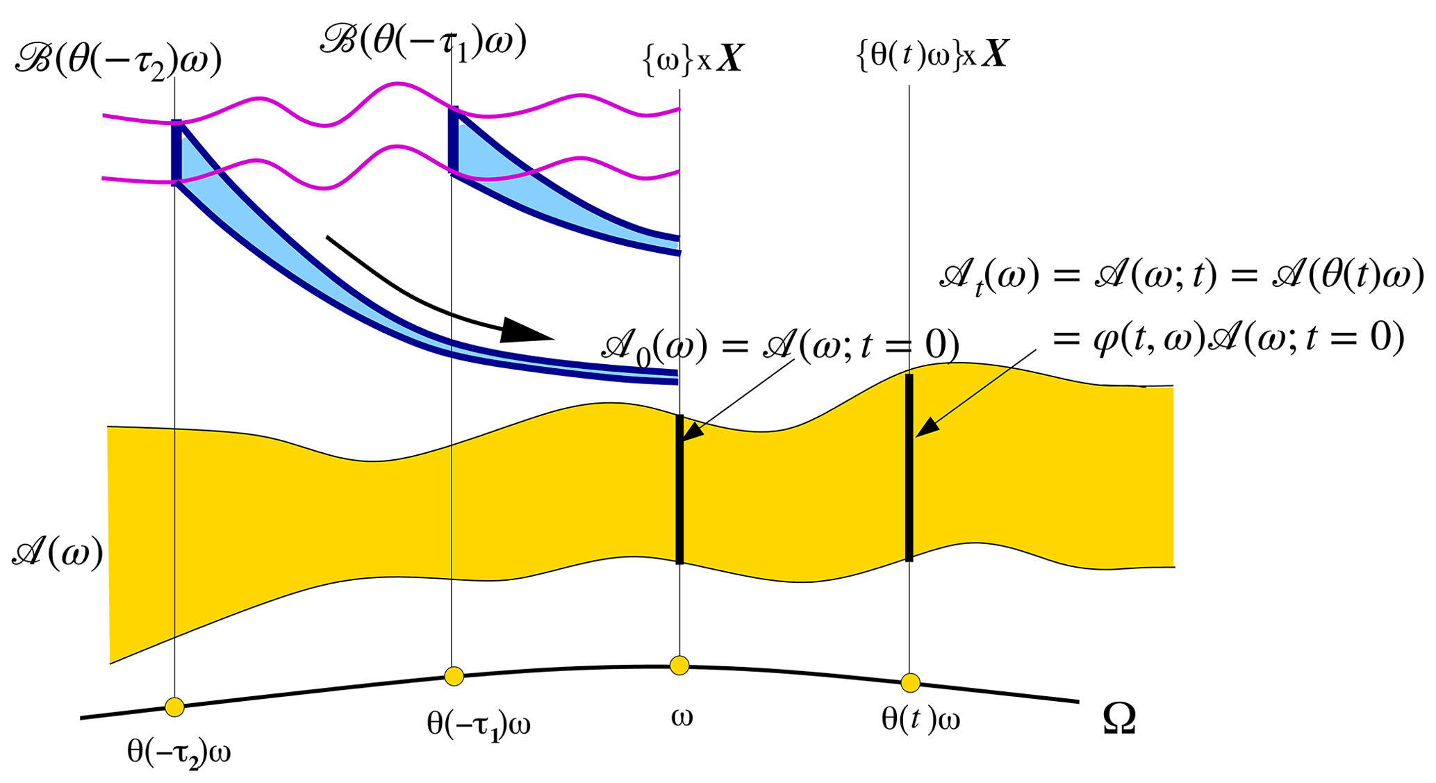
Figure 7 Schematic diagram of a random attractor (ω) and of the pullback attraction to it; here ω labels the particular realization of the random process θ(t)ω that drives the system. We illustrate the evolution in time t of the random process θ(t)ω (light solid black line at the bottom), the random attractor (ω) itself (yellow band in the middle), with the snapshots ${\mathcal{A}}_{\mathrm{0}}\left(\mathit{\omega }\right)=\mathcal{A}(\mathit{\omega };t=\mathrm{0}))$ and 𝒜(ω;t) (the two vertical sections, heavy solid lines), and the flow of an arbitrary compact set ℬ from “pullback times” $t=-{\mathit{\tau }}_{\mathrm{2}}$ and $t=-{\mathit{\tau }}_{\mathrm{1}}$ onto the attractor (heavy blue arrows). See Ghil et al. (2008, Appendix A) for the requisite properties of the random process θ(t)ω that drives the RDS formulated by Eq. (20). Adapted from Physica D: Nonlinear Phenomena, 237, Ghil et al. (2008), Climate dynamics and fluid mechanics: natural variability and related uncertainties, 2111–2126, © 2008 Elsevier B.V. All rights reserved. 2008, with permission from Elsevier.

A key feature of the pullback point of view on noise-perturbed dynamical systems that characterizes RDS theory is the use of a single noise realization, as opposed to the traditional, forward viewpoint of the Fokker–Planck equation and associated concepts, in which multiple noise realizations play a role. For a precise definition of a random attractor – as well as the commonalities and differences between the deterministic and random cases of time-dependent forcing – please see Caraballo and Han (2017).

Chekroun et al. (2011) studied a specific case of such a random attractor for the paradigmatic, climate-related Lorenz (1963) convection model. The authors introduced multiplicative noise into each of the ODEs of the original, deterministically chaotic system, as shown below:

$$\begin{array}{}\text{(21a)}& {\displaystyle }\text{d}X=P_r(Y-X)\text{d}t+\mathit{\sigma }X\text{d}\mathit{\eta },\text{(21b)}& {\displaystyle }\text{d}Y=(rX-Y-XZ)\text{d}t+\mathit{\sigma }Y\text{d}\mathit{\eta },\text{(21c)}& {\displaystyle }\text{d}Z=(-bZ+XY)\text{d}t+\mathit{\sigma }Z\text{d}\mathit{\eta },\end{array}$$

where r=28, P_r=10, and $b=\mathrm{8}/\mathrm{3}$ are the standard parameter values for chaotic behavior in the absence of noise and σ is a constant variance of the Wiener process that is not necessarily small; both the noise realization η(t) and σ are the same in all three equations. The well-known strange attractor of the deterministic case is replaced by the Lorenz model's random attractor, dubbed LORA by the authors. Four snapshots 𝒜_t(ω) of LORA are plotted in Fig. 8 and a video of its evolution in time $\left(\mathit{\omega }\right)=\mathit{\left\{}{\mathcal{A}}_t\right(\mathit{\omega }){\mathit{\}}}_{t\in \mathbb{R}}$ is available as supplementary material to Chekroun et al. (2011) at https://doi.org/10.1016/j.physd.2011.06.005.

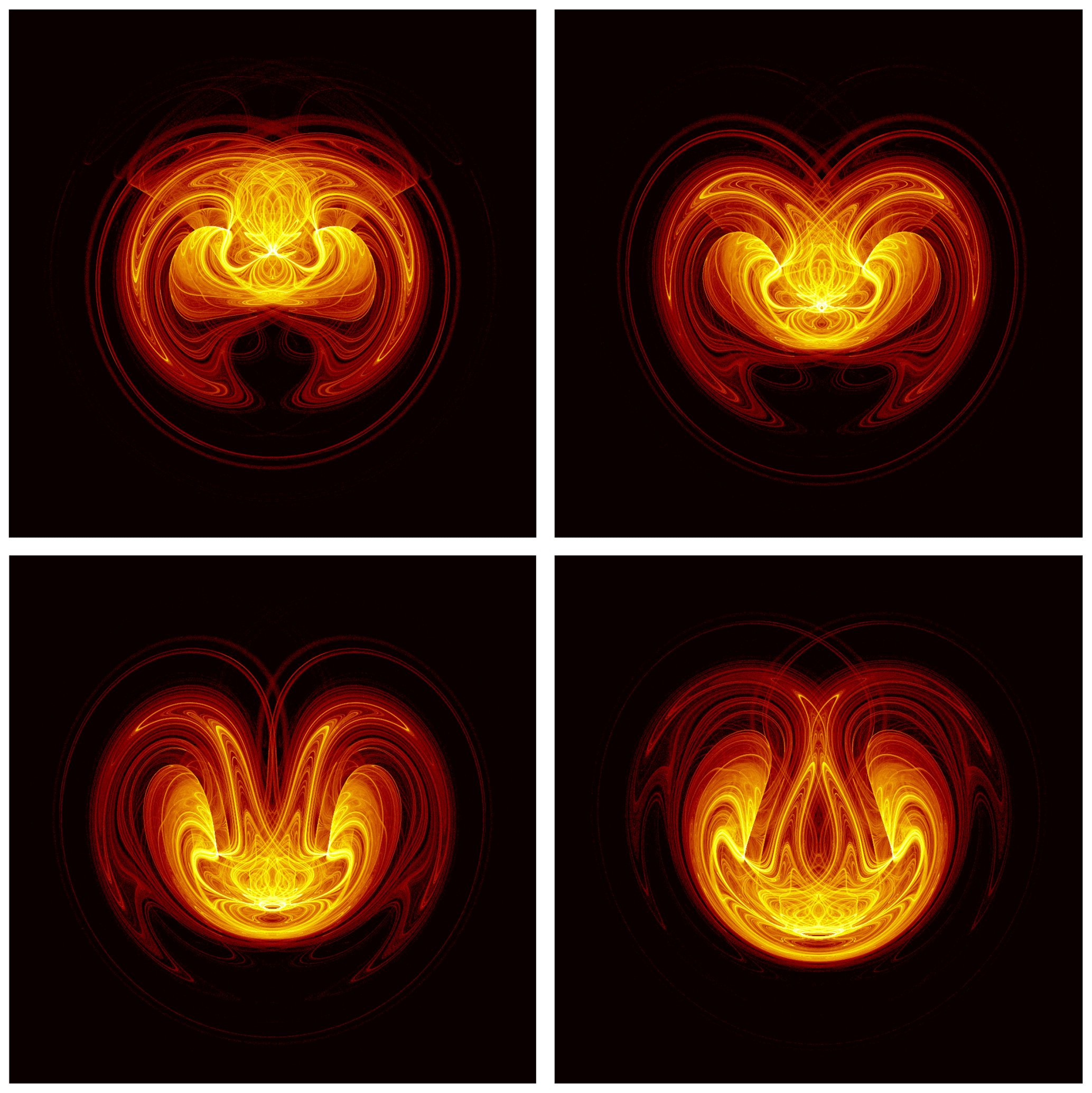
Figure 8 Heat maps of the time-dependent invariant measure ν_t(ω) supported on four snapshots (ω) of LORA. The values of the parameters r, s, and b are the classical ones, where the variance of the noise σ=0.5. The color bar is on a log scale, and it quantifies the probability of landing in a particular region of phase space; a projection is shown of the 3-D phase space $(X,Y,Z)$ onto the (X,Z) plane. Note the complex, interlaced filament structures between highly populated regions (in yellow) and moderately populated ones (in red). Reprinted from Physica D: Nonlinear Phenomena, 240, Chekroun et al. (2011), Stochastic climate dynamics: Random attractors and time-dependent invariant measures, 1685–1700, © 2011 Elsevier B.V. All rights reserved. 2011, with permission from Elsevier.

Charó et al. (2021) have further analyzed the striking effects of the noise on the nonlinear dynamics that are visible in Fig. 8 and in the video of Chekroun et al. (2011) and gathered further insights into the abrupt changes of the snapshots' topology at critical points in time. These remarkable changes suggest the possibility of random processes giving rise to qualitative jumps, such as the MPT, in paleoclimatic variability.

3.3 Application to Dansgaard–Oeschger (D-O) events

Before discussing conceptual glacial cycle models, we take a little detour and introduce a simpler – yet interesting and at the same time highly instructive – application of NDS theory to another important climate phenomenon. During past glacial periods, Greenland experienced a series of sudden decadal-scale warming events that left a clear trace in ice core records (Dansgaard et al., 1993). These so-called D-O events were followed by intervals of steady moderate cooling, before a short phase of enhanced cooling brought the temperatures back to their pre-event levels (e.g., Rasmussen et al., 2014). This pattern is very clearly apparent in NGRIP δ¹⁸O records (North Greenland Ice Core Project members, 2004), and it can be qualitatively simulated by the fast component of a FitzHugh–Nagumo (FHN) model (FitzHugh, 1961; Nagumo et al., 1962), as pointed out by Mitsui and Crucifix (2017), among others; see also Kwasniok (2013), Rial and Yang (2007), Roberts and Saha (2017), and Vettoretti et al. (2022).

We discuss the example of the FHN model at some length in order to illustrate how external forcing can act on a system's internal variability and thereby give rise to more complex dynamics. This model's concise mathematical formulation and its widespread application in paleoclimate modeling and other fields make it ideally suited for this goal. We start with a description of the autonomous model with no time-dependent forcing. Subsequently, we introduce a simple sinusoidal forcing and numerically compute the corresponding PBA. We then extend these consideration into the realm of random dynamical systems by adding stochastic forcing and discuss the resulting random attractor. Finally, we replace the synthetic forcings by one that corresponds to a paleoclimate proxy record of past CO₂ concentrations retrieved from Antarctic ice cores (Bereiter et al., 2015a) and show that this setup brings the model's trajectories into good qualitative agreement with the D-O patterns observed in δ¹⁸O records from Greenland ice cores. In doing so, we pay less attention to the physical interpretation of the model's variables, while focusing on the detailed explanation of model behavior and on the role of the forcing in the resulting dynamics.

3.3.1 The FitzHugh–Nagumo (FHN) model of fast–slow oscillations

The FHN model consists of two coupled ODEs that govern behavior alternating between slow evolutions and fast transitions. Typically, the timescales of the two variables are separated by introducing the parameters τ_x and τ_y, with x(t) being the slow component and y(t) the fast one:

$$\begin{array}{}\text{(22a)}& {\displaystyle }\dot{x}={\displaystyle \frac{\mathrm{1}}{{\mathit{\tau }}_x}}(y-\mathit{\gamma }),\text{(22b)}& {\displaystyle }\dot{y}={\displaystyle \frac{\mathrm{1}}{{\mathit{\tau }}_y}}\left[\mathit{\alpha }\right(y-y^{\mathrm{3}})-x].\end{array}$$

In order to develop an understanding for the way that such a model can simulate the rapid D-O warmings, followed by slow coolings, we start by discussing its autonomous behavior for time-independent γ.

First, consider the case of large timescale separation

$$\begin{array}{}\text{(23)}& {\mathit{\tau }}_x\gg {\mathit{\tau }}_y.\end{array}$$

This choice guarantees that the fast y component adjusts adiabatically to quasi-static changes of the slow x component. The time derivative of y(t), as shown in Fig. 10a, exhibits either three real roots or a single one, depending on the value of x(t), which shifts the graph of the cubic polynomial $P_{\mathrm{3}}(x,y)=\mathit{\alpha }(y-y^{\mathrm{3}})-x$ globally upwards or downwards. Of the three potential roots, the outer two are stable fixed points for y(t) at a fixed value of x, while the inner one is unstable. Note that the two stable fixed points are always located either left or right of the local minimum or maximum of P₃(x,y), respectively. Accordingly, we label them y_l and y_r. The positions of the local extrema, namely $y_{\text{min}}=-\sqrt{\mathrm{1}/\mathrm{3}}$ and $y_{\text{max}}=\sqrt{\mathrm{1}/\mathrm{3}}$, provide an upper and a lower bound for the left and right stable fixed point, respectively.

Now, let us investigate the coupled dynamics of the slow and fast variables x(t) and y(t). Assume we are in a state where $x>\mathrm{2}\mathit{\alpha }/\sqrt{\mathrm{27}}$ such that y_l is the only root of P₃(x,y). Provided that $\left|\mathit{\gamma }\right|<\sqrt{\mathrm{1}/\mathrm{3}}$, the time derivative $\dot{x}$ and x itself will have opposite signs, with the consequence that a slow adjustment process of x(t) sets in. This will shift the polynomial P₃(x,y) upwards in Fig. 10a, which in turn revives the other two roots of P₃(x,y). The fast y(t) closely follows y_l, which is shifted accordingly. Once $x\left(t\right)=-\mathrm{2}\mathit{\alpha }/\sqrt{\mathrm{27}}$, the root y_l stops existing and a fast transition to the neighborhood of the opposite root y_r ensues. This transition switches the sign of $\dot{x}\left(t\right)$ and the slow adjustment of x(t) now happens in the opposite direction.

In the (x,y) plane, this behavior manifests itself as a stable limit cycle. However, any value $\left|\mathit{\gamma }\right|>\sqrt{\mathrm{1}/\mathrm{3}}$ prevents $\dot{x}\left(t\right)$ from switching sign and therefore interrupts the cyclic destruction and revival of the respective opposite root of P₃(x,y). Instead, $\left|\mathit{\gamma }\right|>\sqrt{\mathrm{1}/\mathrm{3}}$ gives rise to a single stable fixed point for the entire system in the (x,y) plane and in this case both variables relax towards it.

In fact, in the autonomous setting, the system's qualitative behavior is controlled by the value of the parameter γ, which decides between internal oscillations along a limit cycle and relaxation towards a fixed point in the (x,y) plane. Note that previously we referred to the roots y_l and y_r also as stable fixed points of y for a given value of x. Here, the term stable fixed point refers to the entire system defined by the coupled ODEs (22a) and (22b). Both $\mathit{\gamma }=\pm \sqrt{\mathrm{1}/\mathrm{3}}$ are critical values of γ that give rise to supercritical Hopf bifurcations of the coupled system's fixed points; recall Fig. 4 of Sect. 2.1.

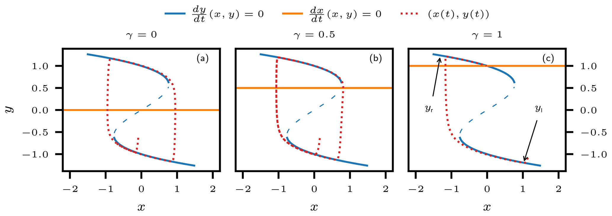
Figure 9 Nullclines of the autonomous FHN model governed by Eq. (22) with large timescale separation, for α=2, τ_x=100, and τ_y=10; the nullclines of the fast y component are in blue, and those of the slow x component are in orange. (a–c) One illustrative trajectory (red dotted) for γ=0, 0.5, and 1.0, respectively. The upper branch and the lower branch of the y nullcline (solid blue) correspond to the roots y_r and y_l, respectively, as defined in the text. For fixed values of x, they constitute stable fixed points for Eq. (22b). The middle branch (dashed blue) corresponds to the unstable fixed point for Eq. (22b) for a given x. The trajectories for panels (a) and (b) follow a limit cycle, as the x nullcline does not intersect with either of the stable branches of the y nullcline, given that $\left|\mathit{\gamma }\right|<\sqrt{\mathrm{1}/\mathrm{3}}$, while the trajectory in panel (c) approaches a single stable fixed point for the coupled system formed by the intersection of the x nullcline with the y_l branch of the y nullcline.

Figure 10 FitzHugh–Nagumo (FHN) model with parameters τ_x=100, τ_y=60, and α=2. (a) The cubic polynomial P₃(x,y) of the fast derivative as a function of y for x=0 (solid blue line); the red lines point to the local maximal and minimal values of P₃(x,y), namely $\pm \mathrm{2}a/\sqrt{\mathrm{27}}$, respectively – these are the maximal values by which P₃ can be shifted up or down, while maintaining all of its three roots; the dotted gray lines indicate the shifted function with $x=\pm \mathrm{2}\mathit{\alpha }/\sqrt{\mathrm{27}}$. The purple lines labeled y_min and y_max mark the right and left boundaries for the roots y_l and y_r, respectively: y_l and y_r can never be located in between the two purple lines. (b) Trajectories of the non-autonomous model with $\mathit{\gamma }\left(t\right)=\mathrm{0.8}\sin (t/{\mathit{\tau }}_{\text{f}})$ and τ_f=1000, plotted in the (x,y) phase plane; the trajectories are colored by their starting times $\mathit{\{}{t}_{\mathrm{0}}=-\mathrm{20}\mathrm{000},t_{\mathrm{1}}=-\mathrm{16}\mathrm{000},t_{\mathrm{2}}=-\mathrm{13}\mathrm{000},t_{\mathrm{3}}=-\mathrm{7000}\mathit{\}}$, and the initial positions were drawn from a standard Gaussian bivariate distribution. (c) The slow time-dependent forcing $\mathit{\gamma }\left(t\right)=\mathrm{0.8}\sin (t/\mathrm{1000})$. (d, e) The same trajectories as in (b) but plotted in time as y=y(t) and x=x(t), respectively. Panels (f–h) are same as panels (c)–(e) but for the fast time-dependent forcing $\mathit{\gamma }\left(t\right)=\mathrm{0.8}\sin (t/\mathrm{350})$​​​​​​​. The gray shading in panels (c)–(h) indicates intervals during which $\left|\mathit{\gamma }\right|>\sqrt{\mathrm{1}/\mathrm{3}}$, and the internal oscillation is hence suppressed.

This behavior can be better understood by considering the nullclines of Eqs. (22b) and (22a) in the (x,y) plane, as shown in Fig. 9. If the branches of the y nullcline that correspond to y_l and y_r, and thus to stable fixed points of Eq. (22b) for a given value of x, intersect with the x nullcline given by y=γ, then this intersection constitutes a stable fixed point for the entire system.

If they do not, the system first relaxes along the fast direction toward the y nullcline. Only then does the adjustment of the slow component start to drag the system along the y nullcline in the direction where the distance to the x nullcline decreases. At the point where the y nullcline reverses, the fast component is immediately attracted by the other branch of the fast nullcline and the same process starts all over again.

So far we have described the formation of the limit cycle in the FHN model under the assumption of clear timescale separation and the independence of the x nullcline {y=γ} from x. See Rocsoreanu et al. (2000) for the emergence of the limit cycle in the more general FHN model.

The highly nonlinear, two-time behavior of the FHN model somewhat modifies the way that stable limit cycles arise in it. While we saw the oscillation's radius grow with the square root of the bifurcation parameter in the case of the normal form given by Eqs. (3)–(5), in the case of the FHN model, the radius of the oscillations actually grows exponentially over a small range of γ values right after the bifurcation point and then stabilizes. These exponentially growing stable limit cycles have been termed “canard cycles” (Benoît, 1983). Roberts and Saha (2017) have pointed out a possible link between canard cycles and D-O cycles, and they play a role in other excitable climate models; see Pierini and Ghil (2022) and references therein.

3.3.2 A pullback attractor of a periodically forced FHN model

Introducing a sinusoidal time dependence

$$\begin{array}{}\text{(24)}& \mathit{\gamma }\to \mathit{\gamma }\left(t\right)\propto \sin (t/{\mathit{\tau }}_{\text{f}})\end{array}$$

into the slow Eq. (22a) makes the system non-autonomous, as discussed in general terms in Sect. 3.2, and it periodically switches the self-oscillatory behavior on and off. We consider here the case in which the variations of the external forcing γ(t;τ_f) occur on a slower timescale than the entire internal dynamics, i.e.,

$$\begin{array}{}\text{(25)}& {\mathit{\tau }}_{\text{f}}>{\mathit{\tau }}_x>{\mathit{\tau }}_y.\end{array}$$

Note that we give up here on the restriction of strict timescale separation between x(t) and y(t), as expressed by Eq. (23).

The trajectories plotted in Fig. 10c–e and f–h represent the solutions of such a periodically forced FHN model starting at different points in the past. The time units are arbitrary and the two sets of solutions are for two different forcing timescales τ_f. These trajectories illustrate the applicability of the pullback perspective suggested by Sect. 3.2 and Fig. 6 to the periodically forced FHN model. In contrast to the illustrative examples of Sect. 3.2, an analytical solution is not available in this case. However, this small sample of numerically computed trajectories, together with the phenomenological discussion herein, is quite sufficient for an intuitive understanding of the system's pullback behavior.

For Fig. 10c–e, the forcing's timescale is much slower then the internal timescales. The amplitude of the forcing γ(t) was chosen such that it repeatedly crosses the two thresholds $\pm \sqrt{\mathrm{1}/\mathrm{3}}$ and thus induces a sequence of Hopf bifurcations by switching between intervals of self-sustained oscillation and attraction to a stable fixed point. Crossing such a bifurcation point due to slow changes in the forcing is referred to as a bifurcation-induced tipping or “B-tipping” (Ashwin et al., 2012; Ghil, 2019; Ghil and Lucarini, 2020).

Strikingly, all trajectories converge to one another during non-oscillatory time intervals, when they are simultaneously attracted by the single existing fixed point. During oscillatory intervals, phase differences between individual trajectories may, in principle, persist. Still, convergence during a single non-oscillatory interval is so strong that after it the trajectories can no longer be discriminated visually. Numerically, however, the distance between trajectories only tends to zero but never reaches it. At the end of non-oscillatory intervals, the trajectories always re-enter the oscillatory regime from the same location in the (x,y) plane – to within negligible numerical differences – and hence very nearly repeat themselves. Qualitatively speaking, the PBA – i.e., the family of invariant snapshots {𝒜(t)}_t∈ℝ of Eq. (13) – is an infinite repetition of the common trajectory structure that can be observed in Fig. 10d, e between −5000 and 15 000 time units. In the case at hand, each snapshot 𝒜(t) consists of a single point.

For Fig. 10f–h, the timescale separation between the forcing and the internal dynamics is reduced, resulting in a qualitatively different behavior of the non-autonomous system. The frequency of occurrence of B-tipping points is much higher, and hence the trajectories do not even execute a full oscillation during a single time interval that permits oscillations. As a result, two stable patterns of trajectories are formed. These two patterns can be brought into agreement by switching the sign of one pattern and shifting it in time by ${\mathit{\tau }}_{\text{f}}/\mathrm{2}$. This symmetry reflects the symmetry of the stable nullcline of the fast system component, as shown in Fig. 9.

Again, the PBA of this non-autonomous system can be thought of as an infinite repetition of the common trajectory structure that can be observed in Fig. 10g, h between −5000 and 15 000 time units. In contrast to the slow-forcing case, each snapshot 𝒜(t) now is comprised of two points in the (x,y) plane. This example illustrates how the action of an external force on an autonomous system can give rise to considerably richer dynamics, which crucially depends on both the system's internal variability and the nature of the forcing.

3.3.3 A random attractor of a periodically and stochastically forced FHN model

Based on the brief introduction to RDSs in Sect. 3.2, we take our investigation of the periodically forced FHN model one step further and include a random component into the external forcing, acting on the model's fast y component:

$$\begin{array}{}\text{(26a)}& {\displaystyle }\text{d}x={\displaystyle \frac{\mathrm{1}}{{\mathit{\tau }}_x}}(y-\mathit{\gamma }(t\left)\right)\text{d}t,\text{(26b)}& {\displaystyle }\text{d}y={\displaystyle \frac{\mathrm{1}}{{\mathit{\tau }}_y}}\left[\mathit{\alpha }\left(y-y^{\mathrm{3}}\right)-x\right]\text{d}t+\mathit{\sigma }\text{d}\mathit{\eta }.\end{array}$$

Here, η denotes a Wiener process, as in Eq. (20) – i.e., a continuous stochastic process whose increments dη are independently and normally distributed, with mean zero and unit variance – and γ(t) remains a periodic forcing of the x component proportional to sin (τ_ft).

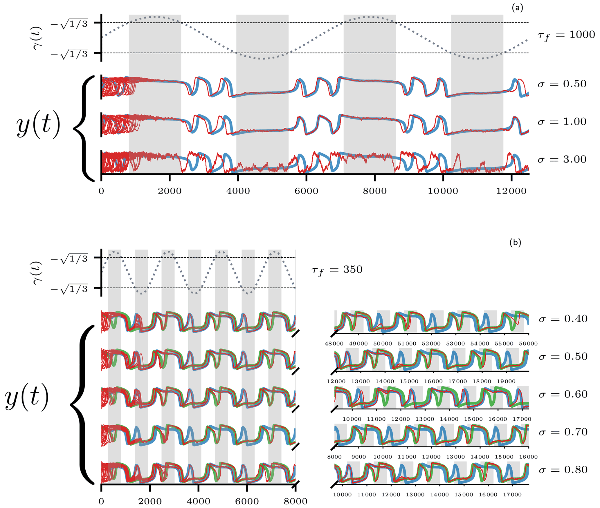
Figure 11 Random attractor of the periodically and stochastically forced FHN model governed by Eq. (26). (a) Results for slow periodic forcing with period τ_f=1000. The top graph shows the periodic forcing, with non-oscillatory intervals marked by gray shading. The next three graphs show the fast y component of the approximate random attractors, as per Eq. (26b); the noise variance σ increases from top to bottom. Each random attractor is approximated by integrating 20 trajectories (solid red) with different initial conditions over time and using the same Wiener process as their common stochastic forcing; the corresponding deterministic PBA is shown in blue. The random attractors and the PBA are very similar for small noise variances, but they differ more and more as the noise variance increases. (b) Results for faster periodic forcing with period τ_f=350. The forcing is only shown for the first 8000 time units, with non-oscillatory intervals again shaded gray. The left part of panel (b) shows five approximate random attractors, computed as in panel (a), on a common time axis. The panel's right-hand side shows their continuations on individual time axes in order to display the moment when full noise-induced synchronization of the trajectories takes place. Prior to this point, the random attractor is split into two branches, which closely follow the PBA of the deterministic system (blue and green). For σ=0.7, the synchronization already takes place during the first 8000 time units.

In order to study the random attractor of this system, we compute trajectories with random initial conditions over a time span long enough to reveal the asymptotic behavior, as shown in Fig. 11. For both the slower and faster deterministic forcing – i.e., τ_f=1000 and τ_f=350, respectively, as studied in the previous paragraphs – several random attractors are approximated for increasing noise variance values σ in Eq. (26b). For each attractor approximation, we use 20 trajectories with the same noise realization. Each random attractor (red) is shown together with the corresponding PBA of the FHN system subject to purely periodic forcing (blue and green).

For the long periodic forcing with τ_f=1000, the trajectories in Fig. 11a converge fairly rapidly to a single one, as in the case with no noise in Fig. 10d, e. Furthermore, there is a clear similarity of pattern and proximity in phase between the PBA of the deterministic system and the random attractor. However, the deviations of the random attractor from the PBA increase in both pattern and phase as the noise variance increases. These deviations are most striking during the oscillatory intervals because the noise can induce phase shifts in the oscillations, which then persist for the duration of the oscillatory interval. During non-oscillatory intervals, the random attractor is less susceptible to the noise because the resulting perturbations decay in the presence of a stable fixed point of the underlying deterministic system.

For the shorter period forcing with τ_f=350, the PBA of the deterministic system features two stable branches, which could in principle persist in the random attractor. As for the case of τ_f=1000, a rapid convergence of the trajectories can be observed for all noise variances. However, two separate bundles of trajectories persist, each associated with one of the two separate branches of the deterministic PBA. Only after some time do the two bundles merge and subsequently follow either one of the two branches of the PBA or the other. This phenomenon is called noise-induced synchronization (e.g., Arnold, 1998; Chekroun et al., 2011). Which of the two PBA branches the random attractor follows depends on the exact noise realization. The random attractor may also switch irregularly from one branch of the PBA to the other (not shown). Already in the simple setup explored here, one notices that the higher the noise variance, the faster the synchronization of the trajectories. This statement must be understood probabilistically: it may certainly happen for two given noise realizations that the random attractor with the higher noise level takes longer to synchronize, as is the case for σ=0.7 and σ=0.8 in Fig. 11b.

The investigation carried out herein assesses a very special case of an FHN model's random attractor. Random attractors of FHN-type models have been studied intensively (e.g., Wang, 2009; Yamakou et al., 2019). Most studies so far, however, have concentrated on the excitable regime of the stochastically forced FHN model, i.e., the deterministic model's parameters were chosen so as to exhibit a single stable fixed point in the absence of the noise. The noise variance was then chosen sufficiently high to ensure that random fluctuations can push the system out of equilibrium and allow it to take a round trip on what would be the deterministic model's limit cycle, given different parameter values. The situation studied here is rather different, as shown across Figs. 9–11.

3.3.4 An FHN model of the NGRIP record

Readers who are familiar with the NGRIP δ¹⁸O record (North Greenland Ice Core Project members, 2004) might have already realized the qualitative resemblance between the proxy data and the fast component's trajectory of the periodically forced FHN model in Fig. 10d. In particular, the prominent sawtooth pattern of the data is satisfactorily captured by the fast and slow dynamics of the model.

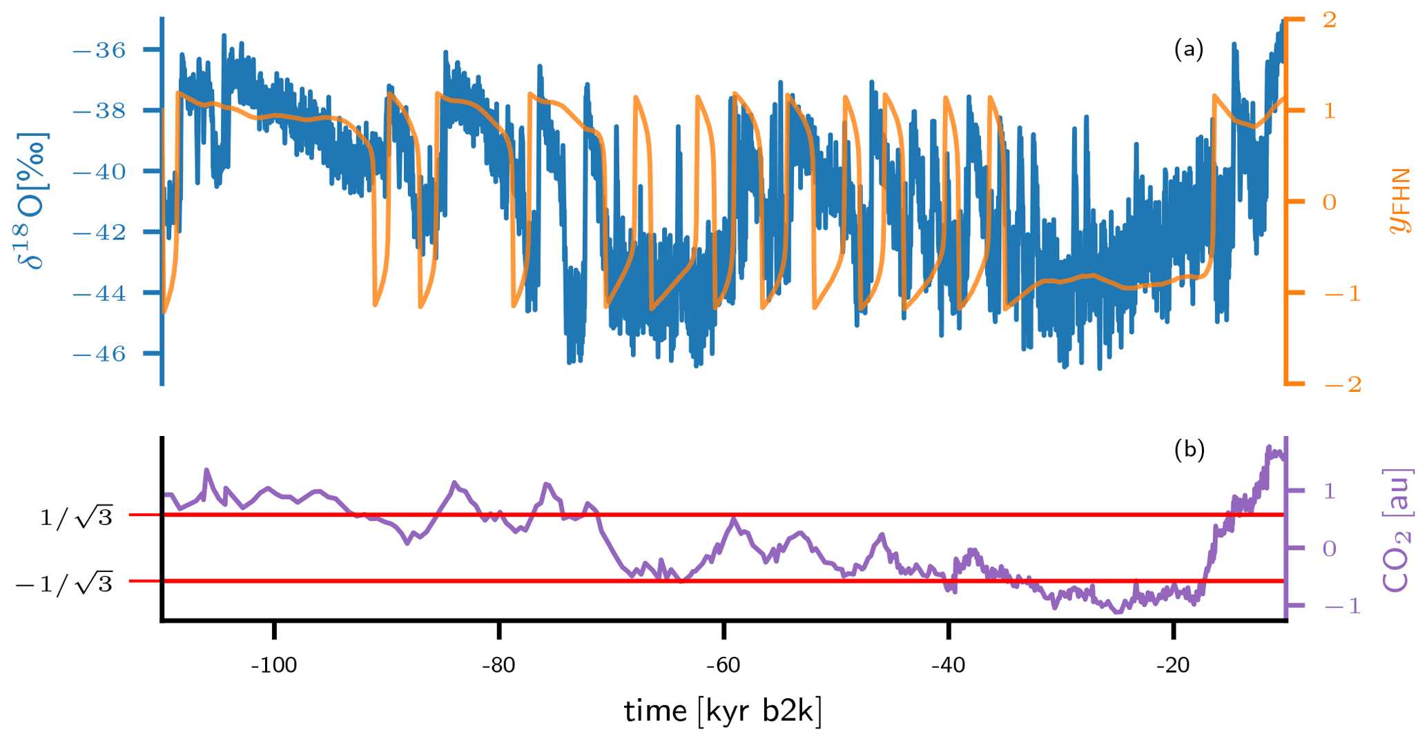
Figure 12 FHN model fit to the NGRIP δ¹⁸O dataset of 20-year means, as published as a supplement to Seierstad et al. (2014) (see also Rasmussen et al., 2014). Originally, the North Greenland Ice Core Project members (2004) reported a 50-year-mean dataset. (a) The fast component y_FHN(t) of an FHN model forced with historical CO₂ concentrations (orange), together with the observed δ¹⁸O record (blue) from the NGRIP ice core (Seierstad et al., 2014). (b) Rescaled atmospheric CO₂ concentrations from Antarctic ice cores in arbitrary units (au) (Bereiter et al., 2015a); the horizontal red lines indicate the lower and upper bounds, $y_{\text{min}}=-\sqrt{\mathrm{1}/\mathrm{3}}$ and $y_{\text{max}}=\sqrt{\mathrm{1}/\mathrm{3}}$, respectively, of the free-oscillation regime.

Figure 12 shows a trajectory of the FHN model for which the sinusoidal forcing used in Fig. 10 was replaced by a rescaled time series of atmospheric CO₂ concentrations retrieved from Antarctic ice cores (Bereiter et al., 2015a):

$$\begin{array}{}\text{(27)}& \mathit{\gamma }\left(t\right)\propto {\mathrm{CO}}_{\mathrm{2}}\left(t\right).\end{array}$$

Is it remarkable how well this simple forcing brings the oscillatory intervals of the FHN model into agreement with the time intervals of the record that are dominated by D-O cycles without any systematic tuning of the model parameters. Clearly, the CO₂-forced FHN model fails to reproduce the exact waiting times between D-O events. However, with these waiting times being at least in part stochastically determined (Ditlevsen et al., 2007), the purely deterministic FHN model is not meant to reproduce the exact pattern of D-O events. Vettoretti et al. (2022) have carried out a detailed study on the use of a CO₂-forced FHN-type model to simulate D-O variability.

In fact, Rousseau et al. (2022, Fig. 6) describe in detail a somewhat more complex, proxy-record-based picture of the interaction between episodes full of D-O events, (Heinrich, 1988) events, and longer-term cooling trends. It is quite possible that a simple model like the one in this section but including explicitly continental ice sheets could capture such a detailed picture.

In the present framework, the FHN model's fast variable y(t) may be interpreted as the intensity of the Atlantic meridional overturning circulation (AMOC), which switches between on and off states during self-oscillatory behavior; see, for instance, Henry et al. (2016), Ghil (1994, Table 5), and Ghil and Lucarini (2020, Table I). The slower x variable that drives the transition between the on and off states of the AMOC may then be taken, for instance, as the waxing and waning of Northern Hemisphere ice sheets (e.g., Ghil et al., 1987), linked in turn to varying ice shelf extent (e.g., Boers et al., 2018), or as the weakening and strengthening of Antarctic bottom water production (Vettoretti et al., 2022).

The interaction between the fast variable and the slow one happens here in the presence of a climate forcing represented by CO₂ concentration. On the much slower timescales of Quaternary glaciations, an interplay between the CO₂ concentration and mean global temperature might also occur, as we shall see in the next section.

4 An NDS for the Quaternary glaciations

Apparently, it was Crucifix (2013) who first applied pullback ideas to the problems of Quaternary glaciations, independently of earlier work on the topic in the climate literature (Ghil et al., 2008; Chekroun et al., 2011; Bódai and Tél, 2012). His work concentrated mainly on the connection between the pacemaking role of the orbital forcing and the observed irregularity of the glacial terminations during the Late Pleistocene; cf. Broecker and Van Donk (1970) and Ghil and Childress (1987, Fig. 11.2).

Based on the considerable success of NDS and RDS applications to other climate problems – such as ENSO (Ghil et al., 2008; Ghil and Zaliapin, 2015; Chekroun et al., 2018; Marangio et al., 2019), the wind-driven ocean circulation (Pierini et al., 2016, 2018), or the evaluation of the ensemble simulations routinely performed in support of the Assessment Reports of the Intergovernmental Panel on Climate Change (Drótos et al., 2015; Vissio et al., 2020) – it would appear worthwhile to proceed further along these lines.

Box 2 summarizes open questions with respect to Quaternary glaciations whose investigation should be aided by NDS and RDS theory. Of course, each of these problems requires one or more distinct climate models, as well as very careful modeling of the kinds of time-dependent changes in forcing and parameters that are most enlightening, as well as most relevant and plausible. A good way would be to start testing ideas with relatively simple models and pursue the investigation systematically across a hierarchy of models – through intermediate ones and on to the most detailed ones – in order to further increase understanding of the climate system and of its predictability on the various paleoclimatic time scales mentioned in the list above.

Box 2 Some open questions concerning Quaternary glaciations.

Such an approach can usefully complement the more common one of merely pushing onwards to higher and higher model resolution in order to achieve ever more detailed simulations of the system's behavior for a limited set of semi-empirical parameter values. Ghil (2001) and Held (2005), among others, have emphasized the need to pursue such a model hierarchy, as originally proposed by Schneider and Dickinson (1974), in order to balance the need to broaden the number of plausible hypotheses vs. the need for confronting them with spatiotemporal details derived from observations.

In this section, we illustrate how the PBA concept can help shed more light upon the dynamics of ice age models. As pointed out in Sect. 3.1 and elsewhere in this paper, there is a long history of modeling the climate of the Quaternary by means of conceptual models, and many non-autonomous models have been proposed to simulate glacial–interglacial cycles of the last 400 kyr to 2.6 Myr based on the orbital forcing. In Appendix A, we provide a long but still not exhaustive list of glacial-cycle models and specify some of their key characteristics, including the degree of their success at simulating the MPT; see also the discussion in Sect. 2.2.

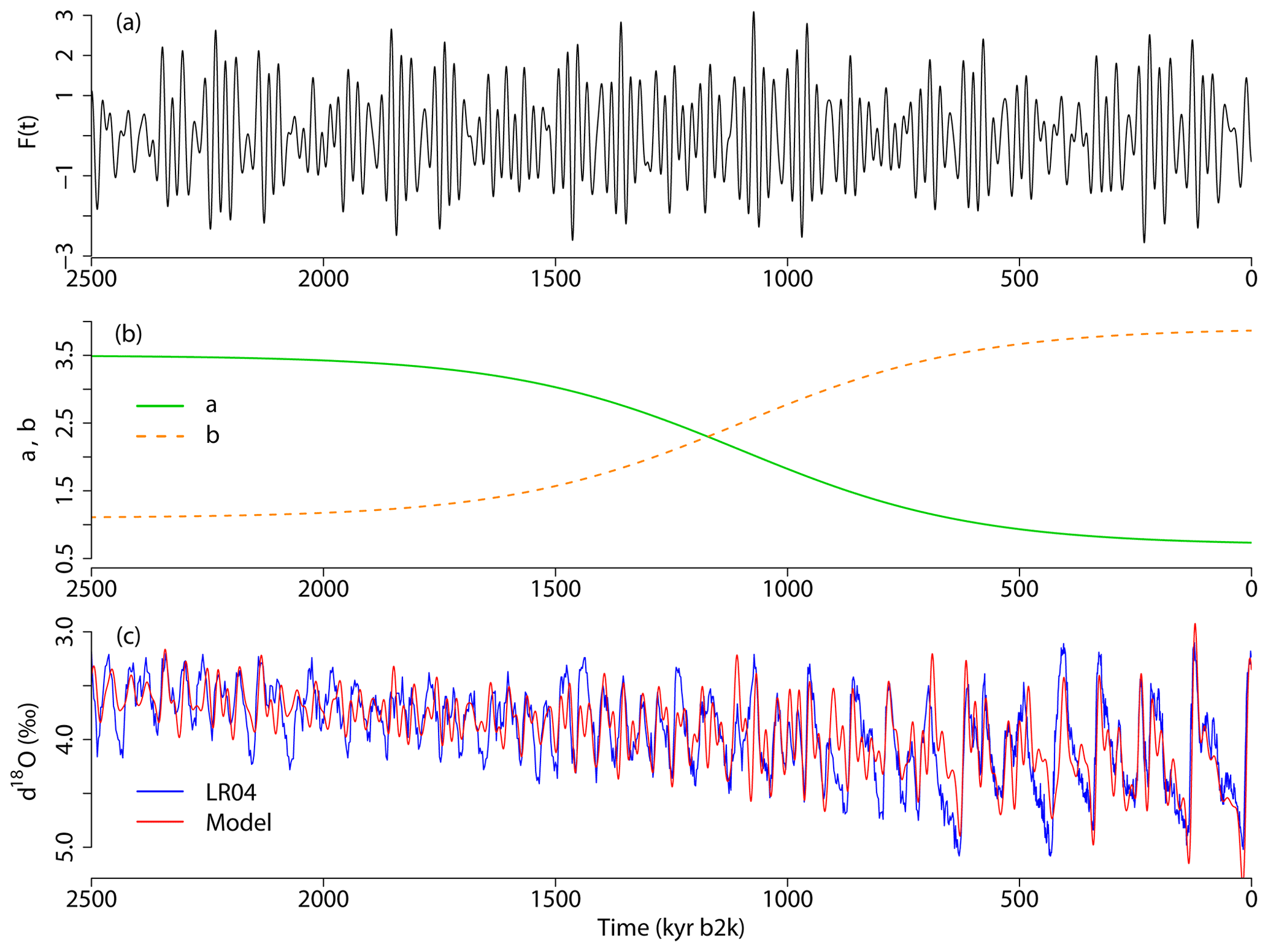
Figure 13 Glacial–interglacial cycles simulated by the modified Daruka and Ditlevsen model of Eqs. (28) and (30): (a) 21 June insolation F(t) at 65^∘ N, normalized to have mean zero and unit standard deviation over the last 1000 kyr, according to Laskar et al. (2004a). (b) Slowly changing parameters α(t) and β(t) introduced to give rise to the MPT. (c) Simulated glacial–interglacial cycles δ¹⁸O_model (red) in comparison with the benthic δ¹⁸O data (blue); the latter dataset, provided by Lisiecki and Raymo (2005a), is also known as the LR04 stack.

Among these glacial-cycle models, the model of Daruka and Ditlevsen (2016, DD16 hereafter) belongs to the more abstract ones, as it is not derived from detailed physical considerations. Still, its concise form, interesting nonlinear dynamics, and ability to simulate glacial cycles, as well as the MPT, make the DD16 model well suited for our illustrative purposes. We first modify this model slightly from its original formulation. We do so mainly in order for the model to better approximate the benthic δ¹⁸O proxy reconstruction of glacial–interglacial cycles due to Lisiecki and Raymo (2005a), especially the timing of glacial terminations; compare our Fig. 13 with Fig. 1 in DD16. Thereafter, we compute the PBAs of the modified DD16 model (hereafter M-DD16) to investigate the dynamical stability of its glacial cycles over the past 2.6 Myr.

Our model's variables, following DD16, are a global temperature anomaly y that is proportional to minus the global ice volume and an effective climatic memory term x that represents the internal degrees of freedom. In the deterministic case, the governing equations of the M-DD16 model are given by

$$\begin{array}{}\text{(28a)}& {\displaystyle }\mathit{\tau }\dot{x}=\mathit{\lambda }y,\text{(28b)}& {\displaystyle }\mathit{\tau }\dot{y}=-\mathit{\alpha }\left(t\right)+x-x^{\mathrm{3}}-\mathit{\beta }\left(t\right)F\left(t\right)x-\mathit{\kappa }y;\end{array}$$

here t is the time (in kyr) and F(t) is the normalized 21 June insolation at 65^∘ N, based on the calculations of Laskar et al. (2004a), as shown in Fig. 13a. The constant parameter values are chosen as κ=1, τ=100, and λ=10. Note that with this choice of λ and unlike in the FHN model of D–O oscillations in Sect. 3.3, x is the fast variable and y is the slow one.

In the original DD16 model, MPT-like behavior was produced by a slow sigmoid variation of the parameter κ in Eq. (28b),

$$\begin{array}{}\text{(29)}& \mathit{\kappa }\left(t\right)={\mathit{\kappa }}_{\mathrm{1}}+\mathrm{0.5}\left({\mathit{\kappa }}_{\mathrm{0}}\mathrm{-}{\mathit{\kappa }}_{\mathrm{1}}\right)\left(\mathrm{1.0}\mathrm{-}\tanh \left({\displaystyle \frac{t\mathrm{-}{t}_{\mathrm{0}}}{t_s}}\right)\right).\end{array}$$

In our M-DD16 model, we introduce instead a slow change in the parameters α(t) and β(t) of Eq. (28b) as follows:

$$\begin{array}{}\text{(30a)}& {\displaystyle }\mathit{\alpha }\left(t\right)=\mathrm{2.1}-\mathrm{1.4}\tanh \left((t+\mathrm{1100})/\mathrm{500}\right),\text{(30b)}& {\displaystyle }\mathit{\beta }\left(t\right)=\mathrm{2.5}+\mathrm{1.4}\tanh \left((t+\mathrm{1100})/\mathrm{500}\right).\end{array}$$

The functions α(t) and β(t) so defined are plotted in Fig. 13b, and they induce, as we shall see forthwith, a change in model behavior that not only resembles the MPT but also shows correct timings for most of the terminations. Moreover, to simulate δ¹⁸O_model, we add a linear trend to the slow variable y to mimic the overall cooling at time scales of millions of years, and thus δ¹⁸O${}_{\text{model}}=\mathrm{4.3}-\mathrm{1.4}y+\mathrm{0.0003}t$. Equation (28) generalizes a first-order ODE system that is equivalent to the Duffing form of the nonlinear spring Eq (7) discussed in Sect. 2.2. The use of such classical first-order systems – like the Duffing and Van der Pol ones – in paleoclimate models was initiated by Saltzman et al. (1981); see also Sect. 2.2 herein.

Figure 13c shows a time series of simulated glacial–interglacial changes δ¹⁸O_model (red) in comparison with the benthic δ¹⁸O (blue) of Lisiecki and Raymo (2005a). The model's initial condition is taken to be $x=-\mathrm{1}$ and y=0 at t=10 000 kyr b2k and, since the insolation forcing in Fig. 13a is prescribed as a time series with 100-year sampling, we solved Eq. (28) using Heun's predictor–corrector method (Isaacson and Keller, 2012, chap. 8) with a step size of 100 years. A large spin-up time is chosen to guarantee that transient effects caused by the initial conditions have abated by the year 2.6 Ma b2k, which is the starting point for the time interval under study. The correlation between the model simulation and the proxy record is 0.75 for the time interval from 2600 to 0 kyr b2k and 0.72 over the interval from 1000 to 0 kyr b2k. Varying the parameters slowly across the time interval of interest, as shown in Fig. 13b, leads to a change in the frequency – from a dominant 41 kyr periodicity prior to the MPT, at roughly 1.2 Ma kyr b2k, to a dominant 100 kyr periodicity after the MPT, at roughly 800 kyr b2k – and a substantial increase in the amplitude.

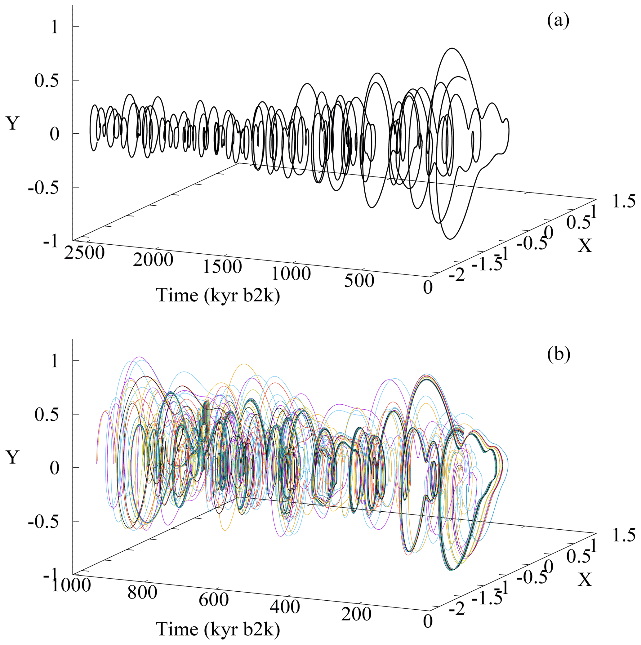
Figure 14 PBA of the M-DD16 model governed by Eq. (28), approximated by 40 trajectories starting from random initial conditions in $(x,y)\in [-\mathrm{2},\mathrm{2}]\times [-\mathrm{2},\mathrm{2}]$ at $t=-\mathrm{10}\mathrm{000}$ kyr. (a) The PBA corresponding to Fig. 13, with the slowly changing parameters α(t) and β(t) given by Eq. (30). (b) The PBA for α(t) and β(t) kept constant at the post-MPT values of α=0.7 and β=3.9. In panel (b), the PBA is shown over a shorter time interval of the last 1000 kyr so that the detailed structure is more clearly visible. Without changes in α and β in time, the overall structure of the PBA is similar before and after 1000 kyr b2k.

We next approximate the PBA by taking 40 random initial conditions at 10 Ma b2k and integrating the model of Eqs. (28) and (30) up to the present time. The PBA in this case is simply a moving fixed point, as plotted in Fig. 14a, since the model dynamics is predominantly stable in the long time interval prior to the MPT. It would thus appear that the orbital forcing simply moves this fixed point around and fully determines Earth's climate. This agrees with the clear statement in DD16 that “first and foremost, our model does not have any internal periods of oscillation”.

However, when keeping the parameters α and β fixed at their post-MPT values α=0.7 and β=3.9 throughout the simulation interval and repeating the computation of the PBA, a more complex picture arises. In the latter case, Fig. 14b shows a bunching of trajectories into separate fuzzy clusters, subject to the quasi-periodic orbital forcing of Fig. 13a.

There are two interesting inferences to be drawn. First, post-MPT dynamics is much more irregular and unstable than the more stable dynamics prior to the MPT. The robustness of the 40 kyr glacial cycles and instability of 100 kyr glacial cycles against perturbations is in line with the conclusions of previous studies (Mitsui et al., 2015; Quinn et al., 2018). It also appears to be consistent with the Willeit et al. (2019) simulation of the last 3 Myr of Earth's history that used an Earth system model of intermediate complexity (CLIMBER-2) that included ice sheets and a carbon cycle, along with atmosphere–ocean dynamics. In their work, trajectories starting from different initial states tended to converge to a single attracting trajectory in the Early Pleistocene, while several distinct trajectories survived in the Late Pleistocene after the MPT.

Second, the separate bundles or “ropes” of trajectories in Fig. 14b seem to point to the type of generalized synchronization discussed in the paleoclimate context by De Saedeleer et al. (2013) and in the context of interannual and interdecadal climate variability by Pierini and Ghil (2022) and Vannitsem et al. (2021). Generalized synchronization in the strict sense of the existence of a map between a time-dependent control and the system's asymptotic behavior has only been shown to hold for non-chaotic systems. Work is under way, however, to further generalize this concept to chaotic systems as well (e.g., Rulkov et al., 1995; Zhang et al., 2007).

5 Conclusions

In this review and research paper, we have covered the contributions of the 1970s to the rebirth of the Milankovitch (1920) theory of the ice ages in Sect. 1 and the 1980s advances in modeling the Quaternary climate's intrinsic variability in Sect. 2. In Sect. 3, we presented first results on the effects of the orbital insolation forcing of the data discussed in Sect. 1 on the intrinsic variability of the data discussed in Sect. 2, and proceeded to introduce the novel concepts and tools of the theory of non-autonomous and random dynamical systems (NDSs and RDSs) that can help to better model and understand these effects. Section 3 concluded with the formulation and study of a FitzHugh–Nagumo (FHN)-type model of recurrent Dansgaard–Oeschger (D-O) events, in which historical CO₂ concentrations induced episodes of D-O events alternating with episodes of their absence in excellent qualitative agreement with NGRIP δ¹⁸O data; see Fig. 12.

Finally, in Sect. 4, we listed a number of open issues on Quaternary and longer paleoclimate timescales and proposed to address them by using the tools of Sect. 3.2. This approach was illustrated by a Duffing-type model of Daruka and Ditlevsen (2016), modified to include slow changes in the parameters that mimic such changes in the Earth system over the duration of the Quaternary period.

When the parameters are gradually changed in time so as to exhibit the mid-Pleistocene transition (MPT), the PBA is simply a moving fixed point. However, when the parameters are fixed at their post-MPT values, the PBA so obtained is chaotic and exhibits clusters of trajectories that we termed ropes. This suggests (a) that the stability of the system is gradually lost while crossing the MPT and (b) that the Late Pleistocene climate, albeit chaotic, may well be subject to a kind of generalized synchronization (cf. De Saedeleer et al., 2013; Pierini and Ghil, 2022; Vannitsem et al., 2021) with the orbital forcing that is illustrated in Fig. 5 of Sect. 3.1 herein. In the specific situation at hand, separate ropes may be associated with various combination tones of the forcing frequencies.

In a broader perspective – and leaving aside various finer points of the MPT conversation outlined in Sect. 2.2 – one can see the work that was reviewed and extended in this paper as a confirmation of the fine intuition of Emiliani and Geiss (1959), 6 decades ago, as summarized in and further expanded by Ghil and Childress (1987, Sect. 12, pp. 446–447).

Hence the following scenario (compare Emiliani and Geiss, 1959) suggests itself for the successive climatic transitions from Pliocene to Pleistocene and from Early to Late Pleistocene: As land masses moved towards more northerly positions, small ice caps formed on mountain chains and at high latitudes. These ice caps, due to their feedback on albedo, made climate more sensitive to insolation variations than it was in the total absence of ice. The response of the climatic system to such variations during the Early Pleistocene (2000 [kyr]–1000 [kyr] ago) was still relatively weak, of a fraction of a degree centigrade in global temperature perhaps, in agreement with the quasi-equilibrium results of Sect. 10.2.

As ice caps passed, about 1000 [kyr] ago, a certain critical size, the unforced system jumped from its stable equilibrium to its stable limit-cycle state (Figures 12.5 and 12.9), increasing dramatically the climate's total variability, to a few degrees centigrade in global temperature. Furthermore, resonant response became possible (see also Oerlemans (1984) [in Berger et al. (1984)] and Sergin (1979)), enhancing abruptly the amplitude of the peak at 100 kyr, among others.

The take-home message is that slow and fast processes, both intrinsic and extrinsic, interact on all paleoclimatic timescales and that we are mastering the art of modeling such interactions.

Appendix A: Low-order dynamical-system models of glacial cycles

The dynamical modeling of glacial cycles dates back to the 1970s. Calder (1974) proposed a model of global ice volume changes that had different sensitivities to the insolation when ice sheets were waxing and waning, respectively. His model can be written as an NDS, according to Paillard (2001). Subsequently, conceptual dynamical models were further developed (e.g., Imbrie and Imbrie, 1980; Berger, 1999). Some of the more recent models simulate the proxy records of glacial cycles remarkably well (Paillard, 1998; Imbrie et al., 2011; Parrenin and Paillard, 2012).

Shortly after Calder (1974) presented his work, Weertman (1976) proposed a simple ice sheet model based on the flow law of a perfectly plastic solid. Next, researchers extended this simple ice sheet model by coupling it with an energy balance model (Källén et al., 1979) and further with the isostatic response of the underlying bedrock (Oerlemans, 1980; Ghil and Le Treut, 1981; Le Treut and Ghil, 1983; Pollard, 1983). Källén et al. (1979) found self-sustained oscillations in their simple coupled ice sheet–energy balance model. Le Treut and Ghil (1983) showed that the dominant 100 kyr periodicity of glacial cycles is generated – in their simple oscillator coupling ice sheet volume with the bedrock's isostatic rebound, on the one hand, and with the atmosphere and ocean's energy balance, on the other hand – via nonlinear resonance with the multi-periodic orbital forcing. More recently, Verbitsky et al. (2018) developed a simple physical model through a scaling argument that respects the underlying physics. Another branch of simple models explicitly includes the carbon cycle as an essential ingredient (Saltzman and Maasch, 1990; Paillard and Parrenin, 2004; Hogg, 2008; Toggweiler, 2008; Omta et al., 2016; Talento and Ganopolski, 2021).

A deeper understanding of glaciation cycles cannot be obtained without process-based models that focus on the detailed physics and biogeochemical phenomena involved (Berger et al., 1999; Ganopolski and Calov, 2011; Abe-Ouchi et al., 2013; Ganopolski and Brovkin, 2017; Willeit et al., 2019). Still, simple dynamical models like the ones mentioned above, as well as models based on more mathematical considerations, are also useful for understanding the climate system's behavior and changes therein, since complex systems can sometimes exhibit familiar dynamics, regardless of the details (Nicolis and Nicolis, 2012; Crucifix, 2011). As Henri Poincaré pointed out, “mathematics is the art of giving the same name to different things”.

Calder (1974)(Paillard, 2001)Weertman (1976)Källén et al. (1979)Ghil and Le Treut (1981)Le Treut and Ghil (1983)Ghil (1994)(Ghil, 1994)(Le Treut and Ghil, 1983)Källén et al. (1979)Ghil and Le Treut (1981)Le Treut and Ghil (1983)Imbrie and Imbrie (1980)Saltzman and Maasch19881990Maasch and Saltzman1990Crucifix (2012)(Mitsui and Aihara, 2014)Paillard (1998)20032012(Paillard, 2001)Paillard (1998)Berger (1999)Paillard and Parrenin2004Ashwin et al. (2018)Ashkenazy and Tziperman (2004)Tziperman et al. (2006)Gildor and Tziperman (2000)Ashkenazy and Tziperman (2004)Källén et al. (1979)Huybers (2007, 2011)(Huybers, 2007)(Huybers, 2011)Huybers (2007)Imbrie et al. (2011)Crucifix (2012)De Saedeleer et al. (2013)(Crucifix, 2012)(Crucifix, 2012)Ashwin et al. (2018)Mitsui et al. (2015)Ashwin and Ditlevsen2015Omta et al. (2016)Daruka and Ditlevsen2016Huybers and Langmuir2017Quinn et al. (2018)Saltzman and Maasch (1988)Ashwin et al. (2018)Paillard and Parrenin (2004)Crucifix (2012)Verbitsky et al. (2018)Talento and Ganopolski2021Benzi et al. (1981, 1982)Nicolis (1981)Benzi et al. (1981, 1982)Nicolis (1981)Matteucci (1989)Pelletier (2003)(Pikovsky and Kurths, 1997)Ditlevsen (2010)Paillard (1998)

Table A1 List of simple conceptual glacial-cycle models with only 1–3 variables. Note that, while extensive, this list is not exhaustive.

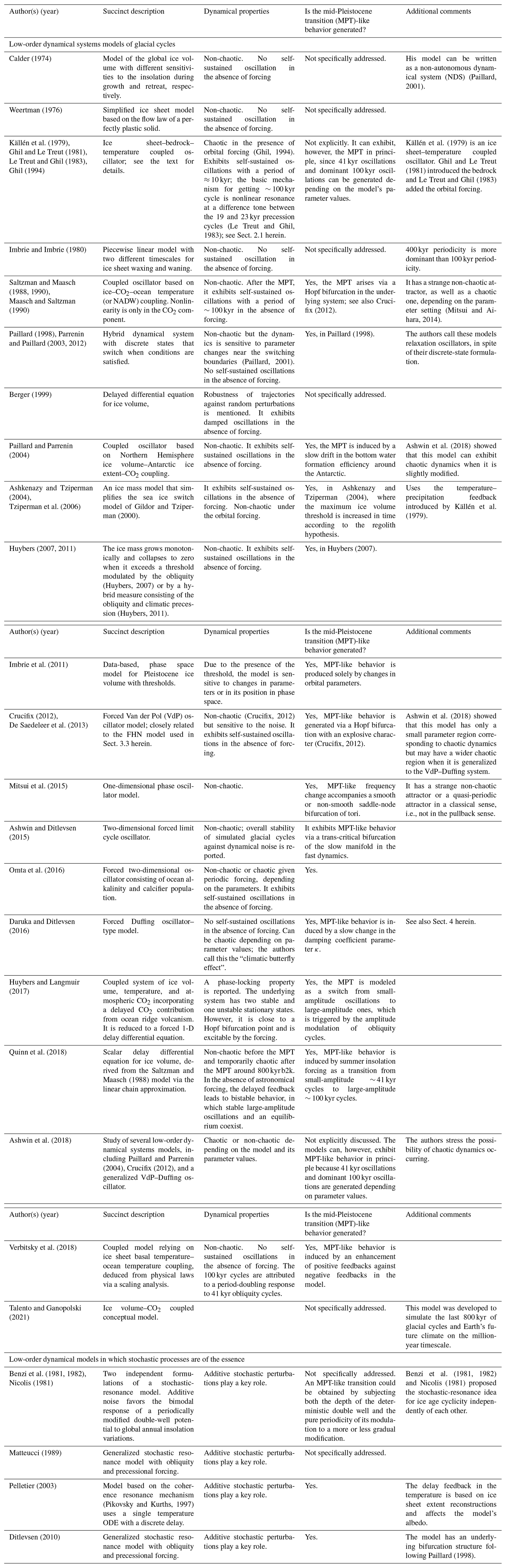
For example, coupled nonlinear oscillators frequently exhibit synchronization with simple frequency ratios, either with each other (Pikovsky et al., 2001) or with the forcing (Ghil and Childress, 1987). Thus, mathematical models that ignore many physical details may also help us elucidate emergent properties in paleoclimatic dynamics (Tziperman et al., 2006; Crucifix, 2011, 2012; De Saedeleer et al., 2013; Mitsui et al., 2015; Ashwin and Ditlevsen, 2015; Daruka and Ditlevsen, 2016) or test different orbital hypotheses (Huybers, 2011). Many low-order models of glacial dynamics are listed in Table A1, although it is by no means exhaustive.

Appendix B: PBA for a limit cycle with sinusoidally modulated radius

Here we study the system of two formally decoupled ODEs

$$\begin{array}{}\text{(B1)}& \begin{array}{rl}& {\displaystyle \frac{\mathrm{d}\mathit{\rho }}{\mathrm{d}t}}=\mathit{\alpha }(\mathit{\mu }+\mathit{\beta }\sin (\mathit{\nu }t)-\mathit{\rho }),\\ & {\displaystyle \frac{\mathrm{d}\mathit{\varphi }}{\mathrm{d}t}}=\mathit{\omega }\text{with}\mathit{\rho }>\mathrm{0},\mathit{\mu }>\mathrm{0},\end{array}\end{array}$$

that were introduced in Sect. 3.2 and analytically derive their invariant sets

$$\begin{array}{}\text{(B2)}& \begin{array}{rl}& \mathcal{A}\left(t\right)=\mathit{\{}\left(\mathit{\alpha }\mathit{\beta }\sin (\mathit{\nu }t+\mathit{\vartheta })+\mathit{\mu },\mathit{\phi }\right):\mathit{\phi }\in [\mathrm{0},\mathrm{2}\mathit{\pi }\left)\mathit{\right\}}\\ & \forall t\in \mathbb{R},\end{array}\end{array}$$

as well as the corresponding pullback attractor (PBA). Following Crauel and Kloeden (2015), the PBA is given by the family

$$\begin{array}{}\text{(B3)}& \textcolor{red}{}=\mathit{\{}\mathcal{A}{\mathit{\}}}_{t:t\in \mathbb{R}}.\end{array}$$

First, we define $\mathrm{\Delta }\mathit{\rho }\left(t\right)=\mathit{\rho }\left(t\right)-\mathit{\mu }$, which gives rise to

$$\begin{array}{}\text{(B4)}& {\displaystyle \frac{\text{d}\mathrm{\Delta }\mathit{\rho }\left(t\right)}{\text{d}t}}=-\mathit{\alpha }\mathrm{\Delta }\mathit{\rho }\left(t\right)+\mathit{\alpha }\mathit{\beta }\sin \left(\mathit{\nu }t\right).\end{array}$$

This is an inhomogeneous ODE and can thus be solved by the variation of parameters method (e.g., Boyce and DiPrima, 2005). The ansatz

$$\begin{array}{}\text{(B5)}& \mathrm{\Delta }\mathit{\rho }\left(t\right)=c\left(t\right)e^{-\mathit{\alpha }(t-t_{\mathrm{0}})},\end{array}$$

yields

$$\begin{array}{}\text{(B6)}& {\displaystyle \frac{\text{d}\mathrm{\Delta }\mathit{\rho }\left(t\right)}{\text{d}t}}=-\mathit{\alpha }\mathrm{\Delta }\mathit{\rho }\left(t\right)+{\displaystyle \frac{\text{d}c\left(t\right)}{\text{d}t}}{e}^{-\mathit{\alpha }(t-t_{\mathrm{0}})}.\end{array}$$

A comparison with Eq. (B4) requires

$$\begin{array}{}\text{(B7)}& {\displaystyle \frac{\text{d}}{\text{d}t}}c\left(t\right)=\mathit{\alpha }\mathit{\beta }\sin \left(\mathit{\nu }t\right)e^{+\mathit{\alpha }(t-t_{\mathrm{0}})},\end{array}$$

and hence

$$\begin{array}{}\text{(B8)}& \begin{array}{rl}c\left(t\right)& =\underset{t_{\mathrm{0}}}{\overset{t}{\int }}\mathit{\alpha }\mathit{\beta }\sin \left(\mathit{\nu }{t}^{\prime }\right)e^{+\mathit{\alpha }(t^{\prime }-t_{\mathrm{0}})}\text{d}{t}^{\prime }+\mathit{\gamma }\\ & ={\left[\mathit{\alpha }\mathit{\beta }\sin \left(\mathit{\nu }{t}^{\prime }\right){\displaystyle \frac{\mathrm{1}}{\mathit{\alpha }}}{e}^{+\mathit{\alpha }(t^{\prime }-t_{\mathrm{0}})}\right]}_{t_{\mathrm{0}}}^t\\ & -\underset{t_{\mathrm{0}}}{\overset{t}{\int }}{\displaystyle \frac{\mathit{\nu }}{\mathit{\alpha }}}\mathit{\alpha }\mathit{\beta }\cos \left(\mathit{\nu }{t}^{\prime }\right)e^{+\mathit{\alpha }(t^{\prime }-t_{\mathrm{0}})}\text{d}{t}^{\prime }+\mathit{\gamma }.\end{array}\end{array}$$

Repeated partial integration yields

$$\begin{array}{}\text{(B9)}& \begin{array}{rl}\underset{t_{\mathrm{0}}}{\overset{t}{\int }}& {\displaystyle \frac{\mathit{\nu }}{\mathit{\alpha }}}\mathit{\alpha }\mathit{\beta }\cos \left(\mathit{\nu }{t}^{\prime }\right)e^{+\mathit{\alpha }(t^{\prime }-t_{\mathrm{0}})}\text{d}{t}^{\prime }=\\ & {\left[{\displaystyle \frac{\mathit{\nu }}{\mathit{\alpha }}}\mathit{\alpha }\mathit{\beta }\cos \left(\mathit{\nu }{t}^{\prime }\right){\displaystyle \frac{\mathrm{1}}{\mathit{\alpha }}}{e}^{+\mathit{\alpha }(t^{\prime }-t_{\mathrm{0}})}\right]}_{t_{\mathrm{0}}}^t\\ & +\underset{t_{\mathrm{0}}}{\overset{t}{\int }}{\displaystyle \frac{{\mathit{\nu }}^{\mathrm{2}}}{{\mathit{\alpha }}^{\mathrm{2}}}}\mathit{\alpha }\mathit{\beta }\sin \left(\mathit{\nu }{t}^{\prime }\right)e^{+\mathit{\alpha }(t^{\prime }-t_{\mathrm{0}})}\text{d}{t}^{\prime }.\end{array}\end{array}$$

Therefore, we find

$$\begin{array}{}\text{(B10)}& \begin{array}{rl}\left(\mathrm{1}+{\displaystyle \frac{{\mathit{\nu }}^{\mathrm{2}}}{{\mathit{\alpha }}^{\mathrm{2}}}}\right)& \underset{t_{\mathrm{0}}}{\overset{t}{\int }}\mathit{\alpha }\mathit{\beta }\sin \left(\mathit{\nu }{t}^{\prime }\right)e^{+\mathit{\alpha }(t^{\prime }-t_{\mathrm{0}})}\text{d}{t}^{\prime }=\\ & {\left[\mathit{\alpha }\mathit{\beta }\sin \left(\mathit{\nu }{t}^{\prime }\right){\displaystyle \frac{\mathrm{1}}{\mathit{\alpha }}}{e}^{+\mathit{\alpha }(t^{\prime }-t_{\mathrm{0}})}\right]}_{t_{\mathrm{0}}}^t\\ & -{\left[{\displaystyle \frac{\mathit{\nu }}{\mathit{\alpha }}}\mathit{\alpha }\mathit{\beta }\cos \left(\mathit{\nu }{t}^{\prime }\right){\displaystyle \frac{\mathrm{1}}{\mathit{\alpha }}}{e}^{+\mathit{\alpha }(t^{\prime }-t_{\mathrm{0}})}\right]}_{t_{\mathrm{0}}}^t,\end{array}\end{array}$$

and finally

$$\begin{array}{}\text{(B11)}& \begin{array}{rl}c\left(t\right)& ={\displaystyle \frac{\mathrm{1}}{\left(\mathrm{1}+\frac{{\mathit{\nu }}^{\mathrm{2}}}{{\mathit{\alpha }}^{\mathrm{2}}}\right)}}\left(\underset{=\mathit{\beta }\left[\sin \left(\mathit{\nu }t\right)e^{\mathit{\alpha }(t-t_{\mathrm{0}})}-\sin \left(\mathit{\nu }{t}_{\mathrm{0}}\right)\right]}{\underbrace{{\left[\mathit{\beta }\sin \left(\mathit{\nu }{t}^{\prime }\right)e^{+\mathit{\alpha }(t^{\prime }-t_{\mathrm{0}})}\right]}_{t_{\mathrm{0}}}^t}}\right.\\ & \left.-\underset{=\frac{\mathit{\nu }\mathit{\beta }}{\mathit{\alpha }}\left[\cos \left(\mathit{\nu }t\right)e^{\mathit{\alpha }(t-t_{\mathrm{0}})}-\cos \left(\mathit{\nu }{t}_{\mathrm{0}}\right)\right]}{\underbrace{{\left[{\displaystyle \frac{\mathit{\nu }\mathit{\beta }}{\mathit{\alpha }}}\cos \left(\mathit{\nu }{t}^{\prime }\right)e^{+\mathit{\alpha }(t^{\prime }-t_{\mathrm{0}})}\right]}_{t_{\mathrm{0}}}^t}}+\mathit{\gamma }\right).\end{array}\end{array}$$

Plugging this result into the ansatz (Eq. B5) yields

$$\begin{array}{}\text{(B12)}& \begin{array}{rl}\mathrm{\Delta }\mathit{\rho }(t,t_{\mathrm{0}})& ={\displaystyle \frac{\mathrm{1}}{\left(\mathrm{1}+\frac{{\mathit{\nu }}^{\mathrm{2}}}{{\mathit{\alpha }}^{\mathrm{2}}}\right)}}\left(\mathit{\beta }\left[\sin \left(\mathit{\nu }t\right)-\sin \left(\mathit{\nu }{t}_{\mathrm{0}}\right)e^{-\mathit{\alpha }(t-t_{\mathrm{0}})}\right]\right.\\ & -\left.{\displaystyle \frac{\mathit{\nu }\mathit{\beta }}{\mathit{\alpha }}}\left[\cos \left(\mathit{\nu }t\right)-\cos \left(\mathit{\nu }{t}_{\mathrm{0}}\right)e^{-\mathit{\alpha }(t-t_{\mathrm{0}})}\right]\right)\\ & +\mathit{\gamma }{e}^{-\mathit{\alpha }(t-t_{\mathrm{0}})},\end{array}\end{array}$$

with the initial conditions

$$\begin{array}{}\text{(B13)}& \mathrm{\Delta }\mathit{\rho }(t_{\mathrm{0}},t_{\mathrm{0}})=\mathit{\gamma }.\end{array}$$

In the pullback limit, all the terms that carry a factor $e^{-\mathit{\alpha }(t-t_{\mathrm{0}})}$ vanish, and thus

$$\begin{array}{}\text{(B14)}& \begin{array}{rl}\underset{t_{\mathrm{0}}\to -\mathrm{\infty }}{lim}\mathrm{\Delta }\mathit{\rho }(t,t_{\mathrm{0}})& ={\displaystyle \frac{\mathrm{1}}{\left(\mathrm{1}+\frac{{\mathit{\nu }}^{\mathrm{2}}}{{\mathit{\alpha }}^{\mathrm{2}}}\right)}}\left(\mathit{\beta }\sin \left(\mathit{\nu }t\right)-{\displaystyle \frac{\mathit{\nu }\mathit{\beta }}{\mathit{\alpha }}}\cos \left(\mathit{\nu }t\right)\right)\\ & =\mathit{\alpha }\mathit{\beta }\sin (\mathit{\nu }t+\mathit{\vartheta }),\end{array}\end{array}$$

with $\mathit{\vartheta }=\arctan (-\mathit{\nu }/\mathit{\alpha })$. For comparison, the modulation of the target radius itself was given by βsin (νt), and hence it is amplified by the factor of α. Since ρ is restricted to positive values, this solution requires αβ<μ.

Since the evolution in time of the phase ϕ(t) is trivial, different initial conditions for the phase do not converge. Hence, the time-dependent sets that are invariant with respect to the dynamics of the system are

$$\begin{array}{}\text{(B15)}& \begin{array}{rl}\mathcal{A}\left(t\right)& =\mathit{\left\{}\right(\mathit{\rho }\left(t\right),\mathit{\varphi }):\mathit{\varphi }\in [\mathrm{0},\mathrm{2}\mathit{\pi }\left)\mathit{\right\}}\\ & =\mathit{\left\{}\right(\mathit{\alpha }\mathit{\beta }\sin (\mathit{\nu }t+\mathit{\vartheta }),\mathit{\varphi }):\mathit{\varphi }\in [\mathrm{0},\mathrm{2}\mathit{\pi }\left)\mathit{\right\}}.\end{array}\end{array}$$

Defined as the indexed family of all 𝒜(t), the system's PBA is comprised of the family of circles

$$\begin{array}{}\text{(B16)}& \begin{array}{rl}\textcolor{red}{}& =\mathit{\left\{}A\right(t){\mathit{\}}}_{t\in \mathbb{R}}\\ & =\mathit{\left\{}\right(\mathit{\alpha }\mathit{\beta }\sin (\mathit{\nu }t+\mathit{\vartheta }),\mathit{\varphi }):\mathit{\varphi }\in [\mathrm{0},\mathrm{2}\mathit{\pi }){\mathit{\}}}_{t\in \mathbb{R}}.\end{array}\end{array}$$