An energy budget approach to understand the Arctic warming during the Last Interglacial

The Last Interglacial period (129–116 ka) is characterised by a strong orbital forcing which leads to a different seasonal and latitudinal distribution of insolation compared to the pre-industrial period. In particular, these changes amplify the seasonality of the insolation in the high latitudes of the Northern Hemisphere. Here, we investigate the Arctic climate response to this forcing by comparing the CMIP6 lig127k and piControl simulations performed with the IPSL-CM6A-LR (the global climate model developed at Institut Pierre-Simon Laplace) model. Using an energy budget framework, we analyse the interactions between the atmosphere, ocean, sea ice and continents.

In summer, the insolation anomaly reaches its maximum and causes a rise in near-surface air temperature of 3.1 ^∘C over the Arctic region. This warming is primarily due to a strong positive anomaly of surface downwelling shortwave radiation over continental surfaces, followed by large heat transfer from the continents to the atmosphere. The surface layers of the Arctic Ocean also receive more energy but in smaller quantity than the continents due to a cloud negative feedback. Furthermore, while heat exchange from the continental surfaces towards the atmosphere is strengthened, the ocean absorbs and stores the heat excess due to a decline in sea ice cover.

However, the maximum near-surface air temperature anomaly does not peak in summer like insolation but occurs in autumn with a temperature increase of 4.2 ^∘C relative to the pre-industrial period. This strong warming is driven by a positive anomaly of longwave radiation over the Arctic Ocean enhanced by a positive cloud feedback. It is also favoured by the summer and autumn Arctic sea ice retreat ($-\mathrm{1.9}\times {\mathrm{10}}^{\mathrm{6}}$ and $-\mathrm{3.4}\times {\mathrm{10}}^{\mathrm{6}}$ km², respectively), which exposes the warm oceanic surface and thus allows oceanic heat storage and release of water vapour in summer. This study highlights the crucial role of sea ice cover variations, Arctic Ocean, as well as changes in polar cloud optical properties on the Last Interglacial Arctic warming.

1 Introduction

In recent years, the Arctic climate system has been undergoing profound changes. Over the last 2 decades, surface air temperature has increased by more than twice the global average (Meredith et al., 2019). This phenomenon, also known as the Arctic amplification, results from complex and numerous interactions involving the atmosphere, land surfaces, ocean and cryosphere (Goosse et al., 2018). Sea ice loss is often cited as one of the main drivers of the Arctic amplification (Serreze and Barry, 2011). Over the past few decades, sea ice cover has responded very quickly to temperature fluctuations. Recent satellite observations reveal large sea ice retreat in September peaking at $-\mathrm{12.8}\pm \mathrm{2.3}$ % per decade (relative to the 1981–2010 mean; Meredith et al., 2019). A striking example is the minimum sea ice extent of 3.74 million km² reported in September 2020 by the NASA Earth Observatory which is the second lowest minimum since the beginning of satellite observations in 1979. During winter months, sea ice changes are smaller (about $-\mathrm{2.7}\pm \mathrm{0.5}\mathit{\%}$ per decade in March; Meredith et al., 2019) but attest to a delayed start of the freezing season. Sea ice cover variations modify the albedo and affect the vertical exchange of heat and water vapour at the atmosphere–ocean interface. These albedo and water vapour effects have been previously analysed in a context of insolation variations, during the last interglacial–glacial transition (Khodri et al., 2005) and the mid-Holocene (Yoshimori and Suzuki, 2019). They also alter the density of oceanic water masses through salt rejection during the ice-growing phase or through freshwater release during the melting period, thereby having the potential to modify the Atlantic Meridional Ocean Circulation (AMOC).

Other studies also highlight the important role of clouds and total water vapour content in amplifying or dampening the Arctic warming (Vavrus, 2004; Shupe and Intrieri, 2004; Vavrus et al., 2009; Graversen and Wang, 2009; Kay et al., 2016). In particular, changes in the amount and characteristics of low-level clouds, i.e. clouds occurring below 2000 m, strongly modulate the shortwave and longwave radiative budgets (Matus and L'Ecuyer, 2017). Remote sensing observations of clouds have shown the importance of cloud partitioning between liquid and ice phases on shortwave radiation received at the Earth's surface (Cesana et al., 2012; Morrison et al., 2011). For a given water content, liquid water droplets are smaller and more abundant than their frozen counterparts. Their structural properties make them more efficient in reflecting incoming solar radiation back to space than ice crystals, which results in a cooling of the surface and the lowest layers of the atmosphere. Moreover, increased low-level cloud cover, trapping longwave emission from the surface, induces a warming of the atmosphere. This effect is more pronounced over newly open waters, where the enhanced moisture flux to the atmosphere contributes to the formation of low-level clouds and leads to enhanced sea ice melt (Palm et al., 2010). These processes are now better captured by climate models, but cloud feedback remains a large source of uncertainty in climate projections (Flato et al., 2013; Ceppi et al., 2017). Another process also contributing to changes in temperature and humidity is the transport of heat and water vapour from low latitudes to the Arctic region (Khodri et al., 2003; Hwang et al., 2011; van der Linden et al., 2019). All these factors interact with each other and make it difficult to understand polar amplification (Serreze and Barry, 2011; Goosse et al., 2018).

The Arctic region also experienced climatic variations during past periods. Investigating past Arctic climate changes could therefore help better understand processes involved in the Arctic amplification. Past interglacial periods are relevant examples for testing key dynamical processes and feedback under temperatures comparable to or warmer than those of the present-day period. Because of the availability of numerous climate reconstructions, the Last Interglacial period, spanning from 129 to 116 ka, has been frequently used. It provides a good testing ground to clarify the relative importance and the cumulative effects of the above mentioned processes. This period is characterised by a strong orbital forcing resulting in a maximum global warming of 2 ^∘C at the peak warmth compared to the pre-industrial period (Turney and Jones, 2010; McKay et al., 2011; Capron et al., 2014). This warming is more pronounced in the high latitudes of the Northern Hemisphere. For the 127 ka period, palaeodata suggest a summer sea surface temperature increase of 1.1±0.7 ^∘C in the North Atlantic compared to the pre-industrial period (Capron et al., 2014, 2017) associated with huge variations of the cryosphere (here, sea ice and ice sheets). In their chronological framework, Thomas et al. (2020) demonstrate that the cryosphere responded early in the Last Interglacial period to the orbital forcing. The sea ice decline started as early as 130 ka and was followed by a retreat of the Greenland ice sheet around 128 ka. Although marine records agree on a significant decline in Arctic sea ice cover during the Last Interglacial period (Brigham-Grette and Hopkins, 1995; Nørgaard-Pedersen et al., 2007; Adler et al., 2009; Stein et al., 2017; Malmierca-Vallet et al., 2018; Kageyama et al., 2021), the presence of perennial or seasonal sea ice cover over the central Arctic Basin is still debated. Among CMIP6 climate models that have run Last Interglacial simulations, only two of them attest to summer ice-free conditions (Kageyama et al., 2021; Guarino et al., 2020).

In addition to Arctic sea ice loss, the Last Interglacial period is characterised by a retreat of both the Greenland and Antarctic ice sheets which have contributed to a sea level rise between 6 and 9 m (Kopp et al., 2009; Dutton et al., 2015).

Palaeorecords indicate that greenhouse gas concentrations at 127 ka were similar to pre-industrial levels. The main difference between the Last Interglacial and the pre-industrial periods results from the astronomical forcing. Changes in obliquity and climatic precession affect both seasonal and annual solar radiation received at the top of the atmosphere. In the high latitudes of the Northern Hemisphere, the strong astronomical forcing leads to increased summer insolation at the top of the atmosphere peaking in June at more than 60 W m⁻² (Fig. 1).

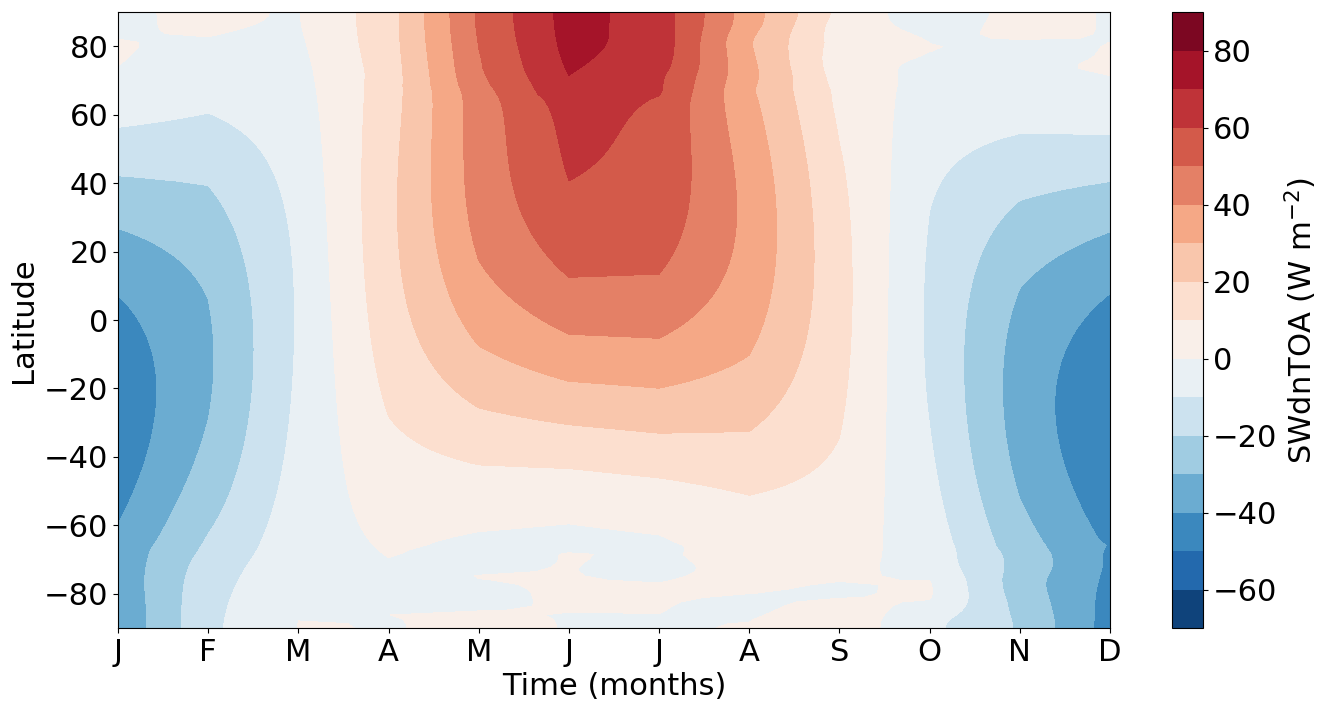
Figure 1 Annual cycle of the insolation LIG–PI anomaly (W m⁻²) as a function of latitudes. The LIG insolation is computed using the celestial calendar with the vernal equinox on 21 March at noon.

Using the Earth system model of intermediate complexity (MoBidiC), Crucifix and Loutre (2002) suggested that during the Last Interglacial, the precession is the main driver of mean annual temperature variations in the high latitudes of the Northern Hemisphere. Changes in summer precession induce significant variations in summer snow cover, sea ice area and vegetation distribution. This modulates surface albedo and is therefore at the origin of most climatic fluctuations in the Arctic. However, while Crucifix and Loutre (2002) have shown that the thermohaline circulation has a limited impact on the high-latitude climate, Pedersen et al. (2016) attributed changes in surface temperature to an increase in the mean annual overturning strength from 15.8 Sv during the pre-industrial period to 21.6 Sv at 125 ka simulated by the high-resolution EC-Earth model. Recently, Guarino et al. (2020) estimated surface heat balance over the Arctic Ocean with the HadGEM3 model to evaluate the link between Arctic warming and loss of summer sea ice at 127 ka. They found a positive anomaly of the net shortwave radiation at the surface, mostly caused by a substantial decrease of surface albedo. Compared with other CMIP6 models, HadGEM3 shows an unusual behaviour in terms of energy budget (Kageyama et al., 2021). The albedo feedback is strongly amplified in this particular model because of the significant summer sea ice retreat. This can be explained by the explicit representation of melt ponds in the CICE-GSI8 sea ice model (Rae et al., 2015; Ridley et al., 2018) which overestimates sea ice melt (Flocco et al., 2012).

These previous studies did not clearly quantify the influence of each climate system components, i.e. ocean, atmosphere, sea ice and continents, that contribute to the Last Interglacial Arctic warming. The aim of this study is to better constrain their respective role based on an energy budget framework. To address this issue, we use the outputs of the IPSL-CM6A-LR (global climate model developed at Institut Pierre-Simon Laplace) global climate model to compare Arctic energy budgets during the Last Interglacial and pre-industrial periods. Moreover, unlike the studies mentioned above, we apply a calendar correction to the model outputs. Due to differences in the Last Interglacial and the pre-industrial orbital forcings, the duration of seasons is different between these two periods. Calendar adjustment is therefore necessary for seasonal analysis (Kutzbach and Gallimore, 1988; Joussaume and Braconnot, 1997; Bartlein and Shafer, 2019).

The paper is organised as follows. Section 2 describes the IPSL-CM6A-LR model and the experimental design of the pre-industrial and Last Interglacial simulations. In Sect. 3, we analyse the processes involved in the Arctic energy budget in order to determine their relative importance in the Arctic warming. We essentially focus on the summer and autumn seasons during which the temperature rise is the highest. Section 4 discusses how model biases could influence our results.

2 Model and methods

2.1 The IPSL-CM6A-LR global model

The simulations analysed in this study were carried out using the IPSL-CM6A-LR model (Boucher et al., 2020). IPSL-CM6A-LR is a global climate model (GCM) developed at the Institut Pierre-Simon Laplace (IPSL). It includes three main components: the atmosphere (the general circulation model developed at the Laboratoire de Météorologie Dynamique, LMDZ; Hourdin et al., 2020), the ocean and sea ice (Nucleus for European Modelling of the Ocean, NEMO; Madec et al., 2019) and the land surface (Organising Carbon and Hydrology In Dynamic Ecosystems, ORCHIDEE; Krinner et al., 2005; Cheruy et al., 2020).

The horizontal resolution of the atmospheric model is 144×143 points in longitude and latitude corresponding to a resolution of $\mathrm{2.5}{}^{\circ }\times \mathrm{1.3}{}^{\circ }$. There are 79 vertical levels reaching 1.5 Pa at the top of the atmosphere. However, we use global fields interpolated on the 19 standard pressure levels defined for CMIP6 (Juckes et al., 2020). The ocean model has a resolution of $\mathrm{1}{}^{\circ }\times \mathrm{1}{}^{\circ }$ and 75 vertical layers. It includes a representation of sea ice (the Louvain-La-Neuve sea ice model, LIM, Vancoppenolle et al., 2008) and geochemistry (the Pelagic Interactions Scheme for Carbon and Ecosystem Studies, PISCES, Aumont et al., 2015). The vegetation model ORCHIDEE uses fractions of 15 different plant functional types. Over ice-free areas, a three-layer explicit snow model is also implemented, whereas over ice sheets and glaciers, the snowpack is represented as a one-layer scheme. Finally, the ORCHIDEE model also includes a carbon cycle representation, which implies that, even though vegetation types are prescribed in each grid box, the seasonal evolution of the leaf area index is computed. The horizontal resolution of ORCHIDEE is the same as that for the atmospheric component.

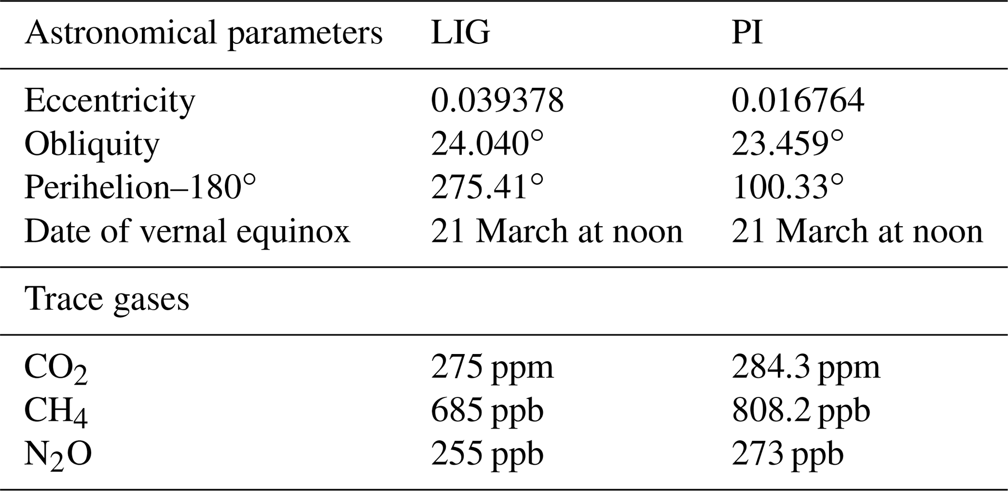
In this study, we use two simulations run as part of the contribution of the fourth phase of Paleoclimate Modelling Intercomparison Project (PMIP4, Kageyama et al., 2018) of the sixth phase of the Coupled Model Intercomparison Project (CMIP6) (Eyring et al., 2016). The piControl experiment for 1850 CE, described in Boucher et al. (2020), is considered our reference simulation and is cited as PI hereafter. The lig127k experiment, hereafter the Last Interglacial (LIG) experiment, is a time-slice experiment corresponding to the 127 ka conditions following the PMIP4 protocol (Otto-Bliesner et al., 2017). As mentioned above, atmospheric CO₂ and other greenhouse gas (GHG) concentrations are close to their PI values and do not represent the main driver of the LIG climate. The LIG GHG concentrations are provided by Antarctic ice cores (Bereiter et al., 2015; Schneider et al., 2013, for CO₂; Loulergue et al., 2008; Schilt et al., 2010a, for CH₄; and Schilt et al., 2010a, b, for NO₂) aligned with the Antarctic Ice Core Chronology 2012 (AICC2012) (Bazin et al., 2013). The Earth's astronomical parameters are prescribed following Berger and Loutre (1991). In all simulations, the vernal equinox is fixed to 21 March at noon. Other boundary conditions such as palaeogeography, ice sheet geometry or aerosols are the same as those in the PI simulation (for more details, see Otto-Bliesner et al., 2017). Forcings and boundary conditions of both simulations are summarised in Table 1.

Table 1 Astronomical parameters and atmospheric trace gas concentrations used to force LIG and PI simulations (from Otto-Bliesner et al., 2017).

The LIG simulation was initialised as the mid-Holocene one (Braconnot et al., 2021). The initial state is the year 1850 (1 January) of the CMIP6 reference pre-industrial simulation with the same model version (Boucher et al., 2020). The model was first run for 350 years. This initial step constitutes the spin-up period, during which the model reaches a statistical equilibrium under the Last Interglacial forcing. From this spin-up phase, the reference PMIP4-CMIP6 lig127k simulation has been run for 550 years. High-frequency outputs have also been saved over the last 50 years of the simulation for the analyses of extreme events and to provide the boundary conditions for future regional simulations. This reference simulation is called CMIP6.PMIP.IPSL.IPSL-CM6A-LR.lig127k.r1i1p1f1 in the ESGF database.

Because of the combined effects of eccentricity and precession changes, the length of seasons relative to the insolation forcing is different between the LIG and the PI periods. However, both simulations use a fixed present-day calendar to compute online monthly averages, which is aligned with our current definition of seasons in terms of number of days for each month. As a consequence, this adds artificial biases in the analysis due to phase lag in the seasonal cycle, especially in boreal autumn (Joussaume and Braconnot, 1997; Timm et al., 2008; Bartlein and Shafer, 2019). To prevent such so-called “palaeo-calendar effects”, we have adjusted the LIG monthly outputs with the PaleoCalAdjust algorithm (Bartlein and Shafer, 2019).

2.2 Climatological evaluation of IPSL-CM6A-LR for the Arctic region

The present-day climate simulated by the IPSL-CM6A-LR model has been evaluated in Boucher et al. (2020). Compared to the IPSL-CM5 model versions, significant improvements have been made for the turbulence, convection and cloud parameterisations (Hourdin et al., 2020; Madeleine et al., 2020). The adjustment of the subgrid-scale orography parameters has helped to correct a systematic bias in the representation of the Arctic sea ice (Gastineau et al., 2020). On an annual basis, this results in a general reduction of temperature biases from IPSL-CM5A-LR to IPSL-CM6A-LR versions (Boucher et al., 2020). In the high latitudes of the Northern Hemisphere, the cold bias in surface air temperature has been considerably reduced over the North Atlantic Ocean, as well as the warm bias over northern Canada. However, surface air temperatures are still too low over the Greenland ice sheet, and a warm bias is also simulated in winter over the Arctic. The latter is associated with an underestimation of sea ice extent also found in summer. Despite these biases, the sea ice cover simulated with IPSL-CM6A-LR is in better agreement with satellite data compared to previous model versions.

The coupled model also tends to underestimate deep water formation in the North Atlantic and associated overturning circulation. In the Northern Hemisphere, the northward heat transport is more intense compared to previous model versions but remains weaker than that deduced from the few available direct observations. As the warm Atlantic and Pacific waters entering the Arctic Basin affect the position of the sea ice front, they may be partly responsible for temperature and sea ice biases mentioned above.

To evaluate the ability of IPSL-CM6A-LR to simulate the Last Interglacial climate, we compare the simulated surface temperature changes with the new data synthesis provided by Otto-Bliesner et al. (2021). We use temperature reconstructions representing annual or summer surface conditions (Fig. 2).

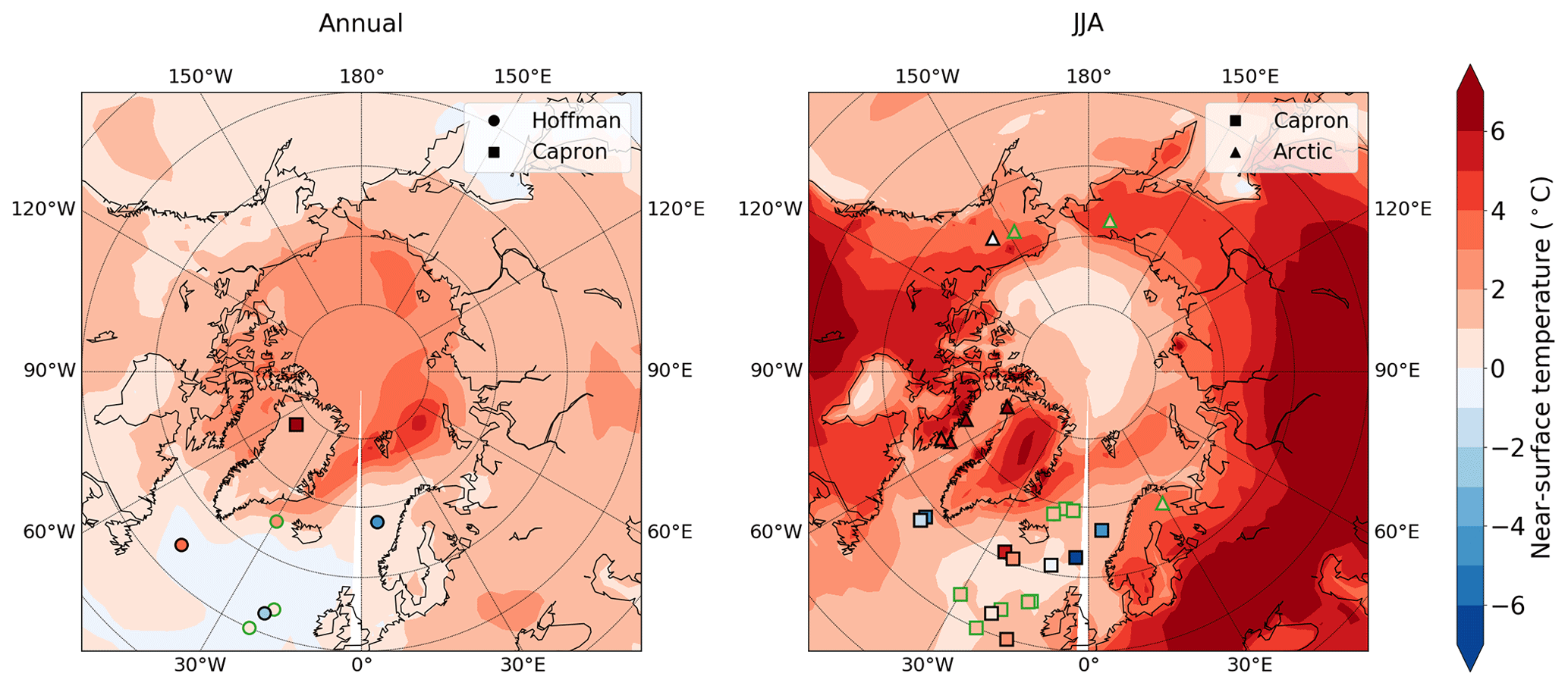
Figure 2 LIG–PI anomaly of the near-surface air temperature (^∘C) simulated by the IPSL-CM6A-LR model (colour shading) and reconstructed from proxy data synthesis (filled markers) as published by Otto-Bliesner et al. (2021). Symbols represent the source of surface air reconstruction: circles for the compilation by Hoffman et al. (2017), squares for the compilation by Capron et al. (2014, 2017) and triangles for the Arctic compilation. Sites showing good model–data agreement (i.e. considering a data uncertainty of ±1σ) are indicated by a green outline.

Marine proxies generally display more heterogeneous LIG–PI changes than model outputs. In summer, the IPSL-CM6A-LR model simulates the surface warming well, but it does not reproduce local cooling in the Labrador and Norwegian seas. This mismatch appears to be a general feature across CMIP5 (Lunt et al., 2013; Masson-Delmotte et al., 2013) and CMIP6 (Otto-Bliesner et al., 2021) models. This has been attributed to uncertainties or simplifications in the specified boundary conditions. Indeed, the PMIP4-CMIP6 protocol consists of setting the ice sheets to their modern configuration and neglects the freshwater inputs to the North Atlantic from ice melting in the LIG simulation. These have been shown to be responsible for local heterogeneities in simulations of the Last Interglacial climate (Govin et al., 2012; Stone et al., 2016): these freshwater fluxes modulate the strength of the AMOC (Swingedouw et al., 2009) and thus the inflow of warm Atlantic waters in the Arctic Ocean. Moreover, comparison with sedimentary data suggests that the IPSL-CM6A-LR model simulates too much sea ice in the Labrador Sea (Kageyama et al., 2021). With a larger sea ice cover in this region, air–sea heat exchange is reduced, which also influences the AMOC intensity (Pedersen et al., 2016; Kessler et al., 2020).

The IPSL-CM6A-LR model and terrestrial data generally agree on the sign of the near-surface temperature anomaly. They often differ on its magnitude, but the amplitude of the reconstructed temperature anomalies is not always consistent for sites close to each other (at the scale of the model's spatial resolution), as is the case in the North Atlantic Ocean in summer. The model does not capture the strong annual warming recorded in the North Greenland Eemian Ice Drilling (NEEM) ice core (NEEM community members, 2013).

By analysing the reasons for Arctic climate change in our simulations, our aim is also to contribute to understand the mechanisms of these climatic changes and how their representation could be improved to obtain better agreement with the reconstructions. In this study, we consider that the model–data agreement is sufficient to investigate the processes contributing to the Last Interglacial Arctic warming.

2.3 Arctic energy budget framework

The energy budget framework has been developed to identify key dynamical processes contributing to the Arctic amplification from observations and reanalyses (Nakamura and Oort, 1988; Semmler et al., 2005; Mayer et al., 2017, 2019; Serreze et al., 2007) or climate models (Rugenstein et al., 2013). We estimate the coupled atmosphere–ocean–land–sea ice energy budget of the Arctic during the LIG and the PI periods based on the work of Mayer et al. (2019) and Serreze et al. (2007).

The seasonal cycle of this energy budget computed from model outputs is averaged over the last 200 years of the simulations to smooth out the interannual and decadal variability. We quantify the heat transfer between the surface and the atmosphere, the oceanic and atmospheric heat transport and the heat storage terms over the Arctic region defined as the area between 60 and 90^∘ N. A schematic representation of the different contributions involved in the energy budget is displayed in Fig. 3. All terms are expressed in W m⁻².

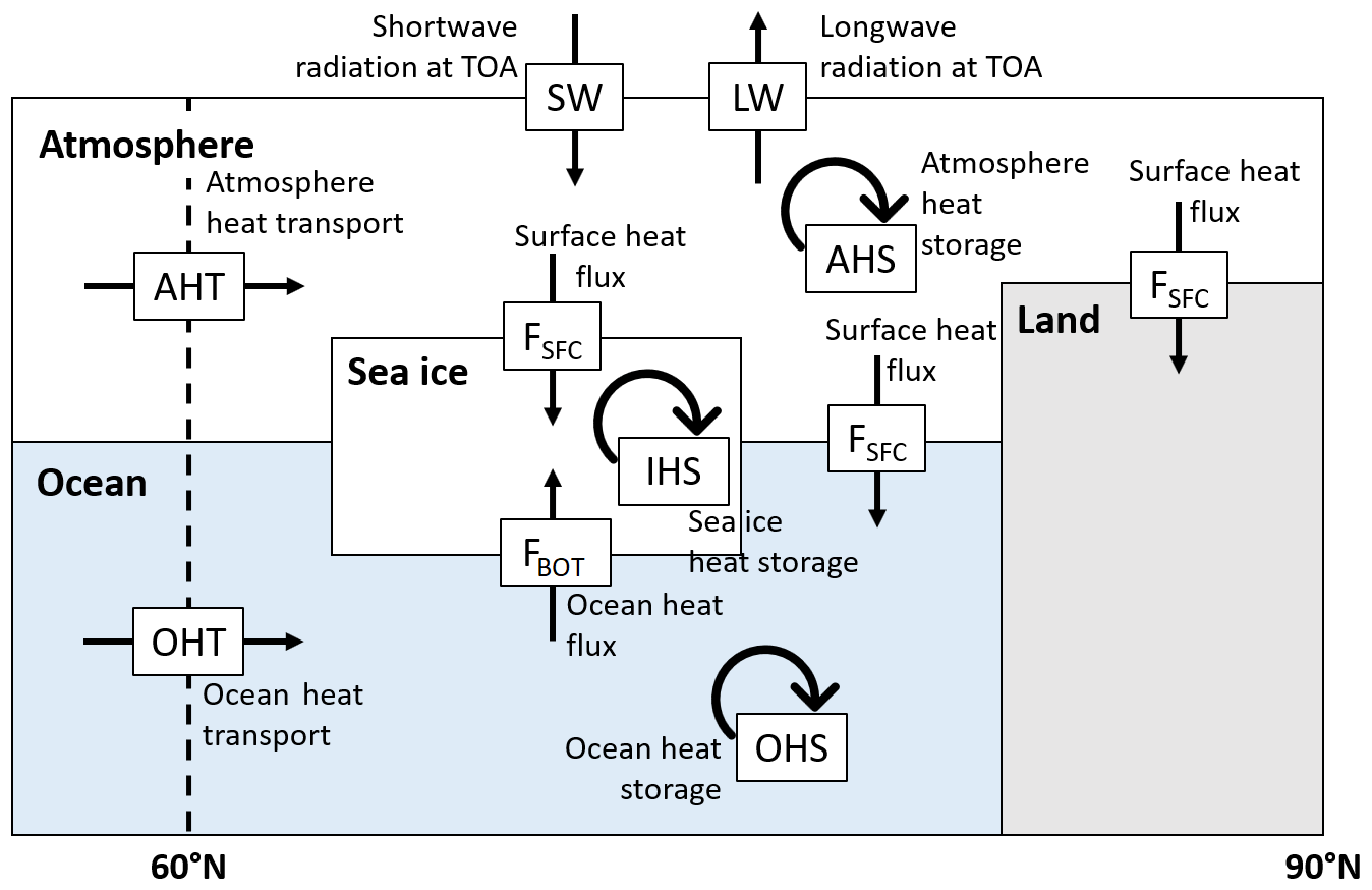
Figure 3 Representation of the different processes involved in the Arctic energy budget: the heat transfer between the surface and the atmosphere (F_SFC), the sea ice–ocean heat flux (F_BOT), the oceanic (OHT) and atmospheric (AHT) heat transport and the heat storage terms (AHS, OHS and IHS).

We consider the energy content of an atmospheric column from the surface to the top (AHC, Eq. 1). It can be expressed as the sum of internal (Cp_aT), kinetic (E_k), latent (L_eq) and potential (ϕ_s) energies. The time derivative of the atmospheric heat content yields the atmospheric heat storage (AHS, Eqs. 2 and 3) which varies with the radiative flux at the top of the atmosphere (F_TOA), surface heat flux (F_SFC) and the heat transport (AHT).

$$\begin{array}{}\text{(1)}& {\displaystyle }\text{AHC}={\displaystyle \frac{\mathrm{1}}{g}}\underset{\mathrm{0}}{\overset{p_{\mathrm{s}}}{\int }}\left({\text{Cp}}_{\mathrm{a}}T+E_{\mathrm{k}}+L_{\mathrm{e}}q+{\mathit{\varphi }}_{\mathrm{s}}\right)\mathrm{d}p\text{(2)}& {\displaystyle }\text{AHS}={\displaystyle \frac{\partial }{\partial t}}{\displaystyle \frac{\mathrm{1}}{g}}\underset{\mathrm{0}}{\overset{p_{\mathrm{s}}}{\int }}\left({\text{Cp}}_{\mathrm{a}}T+E_{\mathrm{k}}+L_{\mathrm{e}}q+{\mathit{\varphi }}_{\mathrm{s}}\right)\mathrm{d}p\text{(3)}& {\displaystyle }\text{AHS}=F_{\mathrm{TOA}}-F_{\mathrm{SFC}}+\text{AHT}\end{array}$$

g is the gravitational acceleration (9.81 m s⁻²), Cp_a is the specific heat of the atmosphere at constant pressure (1005.7 J  K⁻¹ kg⁻¹), T is the temperature (in Kelvin), E_k is the kinetic energy computed as $\frac{u^{\mathrm{2}}+v^{\mathrm{2}}}{\mathrm{2}}$ (in m² s⁻²), L_e is the latent heat of evaporation (2.501×10⁶ J kg⁻¹), q is the specific humidity (in kg kg⁻¹, ϕ_s is the surface geopotential (in m² s⁻²), p is the pressure (in Pa), and p_s is the surface pressure (in Pa).

The surface flux (F_SFC, Eq. 4) can be broken down into downwelling shortwave radiation (SW_dnSFC), upwelling shortwave radiation (SW_upSFC), downwelling longwave radiation (LW_dnSFC), upwelling longwave radiation (LW_upSFC), latent heat flux (f_lat) and sensible heat flux (f_sens).

$$\begin{array}{}\text{(4)}& \begin{array}{rl}{F}_{\mathrm{SFC}}=& {\text{SW}}_{\mathrm{dn}}\text{SFC}-{\text{SW}}_{\mathrm{up}}\text{SFC}+{\text{LW}}_{\mathrm{dn}}\text{SFC}\\ & -{\text{LW}}_{\mathrm{up}}\text{SFC}+f_{\mathrm{lat}}+f_{\mathrm{sens}}\end{array}\end{array}$$

Finally, the energy flux at the top of the atmosphere (F_TOA) is equal to the difference between upwelling and downwelling radiative fluxes:

$$\begin{array}{}\text{(5)}& F_{\mathrm{TOA}}={\text{SW}}_{\mathrm{dn}}\text{TOA}-{\text{SW}}_{\mathrm{up}}\text{TOA}-{\text{LW}}_{\mathrm{up}}\text{TOA}.\end{array}$$

As for the atmosphere, the energy content of the ocean (OHC, Eq. 6) is integrated from the surface to the bottom of the oceanic column (Eqs. 7 and 8).

$$\begin{array}{}\text{(6)}& \text{OHC}={\mathit{\rho }}_{\mathrm{w}}{\text{Cp}}_{\mathrm{w}}\underset{\mathrm{0}}{\overset{z}{\int }}{T}_{\mathrm{cons}}\mathrm{d}z\end{array}$$

$$\begin{array}{}\text{(7)}& \text{OHS}={\mathit{\rho }}_{\mathrm{w}}{\text{Cp}}_{\mathrm{w}}{\displaystyle \frac{\partial }{\partial t}}\underset{\mathrm{0}}{\overset{z}{\int }}{T}_{\mathrm{cons}}\mathrm{d}z\end{array}$$

$$\begin{array}{}\text{(8)}& \text{OHS}=F_{\mathrm{SFC}}\times f_{\mathrm{oce}}-F_{\mathrm{BOT}}\times f_{\mathrm{ice}}+\text{OHT}\end{array}$$

f_oce is the ocean area fraction, f_ice is the sea ice area fraction, ρ_w is the seawater density (1035 kg m⁻³), Cp_w is the specific heat of the ocean at constant pressure (J K⁻¹ kg⁻¹), T_cons is the seawater conservative temperature (in Kelvin), and z is the depth (in m). We use the seawater conservative temperature because it better represents the oceanic heat content than the seawater potential temperature (Intergovernmental Oceanographic Commission et al., 2010). In Eqs. (2) and (7), we use a monthly time step to derive the atmosphere and ocean heat content, respectively.

The sea ice bottom heat flux (F_BOT) represents the heat exchange between the ocean and sea ice. It is defined as the difference between the ocean heat flux (F_OCE) and the conductive heat flux (F_COND) at the bottom of the sea ice cover (Eq. 9).

$$\begin{array}{}\text{(9)}& F_{\mathrm{BOT}}=F_{\mathrm{OCE}}-F_{\mathrm{COND}}\end{array}$$

The sea ice heat content results primarily from heat exchange with the atmosphere and the ocean. The heat flux derived from the sea ice transport (IHT) from regions of ice formation to regions of ice melt is included in the calculation of the sea ice heat storage (IHS, Eq. 10).

$$\begin{array}{}\text{(10)}& \text{IHS}=F_{\mathrm{SFC}}\times f_{\mathrm{ice}}+F_{\mathrm{BOT}}\times f_{\mathrm{ice}}+\text{IHT}\end{array}$$

For terrestrial regions, the energy budget variations are only due to changes in F_SFC over the continents. Lateral heat transport divergences are small and can be ignored (Serreze et al., 2007). Thus, the storage term is equal to the air–land heat exchange.

We choose the same sign convention for all fluxes; i.e. positive fluxes point downward. They act to warm the surface when they are positive except for F_BOT, which cools the sea ice when positive.

Ocean, atmosphere and sea ice transport is computed as the residual of the surface heat fluxes, the bottom heat flux and the heat storage term. From Eqs. (3), (8) and (10), we can write

$$\begin{array}{}\text{(11)}& {\displaystyle }\text{AHT}=\text{AHS}+F_{\mathrm{SFC}}-F_{\mathrm{TOA}}\text{(12)}& {\displaystyle }\text{OHT}=\text{OHS}-F_{\mathrm{SFC}}\times f_{\mathrm{oce}}+F_{\mathrm{BOT}}\text{(13)}& {\displaystyle }\text{IHT}=\text{IHS}-F_{\mathrm{SFC}}\times f_{\mathrm{ice}}-F_{\mathrm{BOT}}.\end{array}$$

These equations give coherent zonally averaged profiles for the PI simulation with a zero northward atmospheric and oceanic heat transport at the North Pole (Fig. 4). To validate this approach, we also compared the mean annual OHT computed as a residual with the OHT computed online by the model (AHT and IHT are not stored in the CMIP6 database). The difference between both methods is around 0.005 PW for the Arctic region, which represents less than 2 % of the model average.

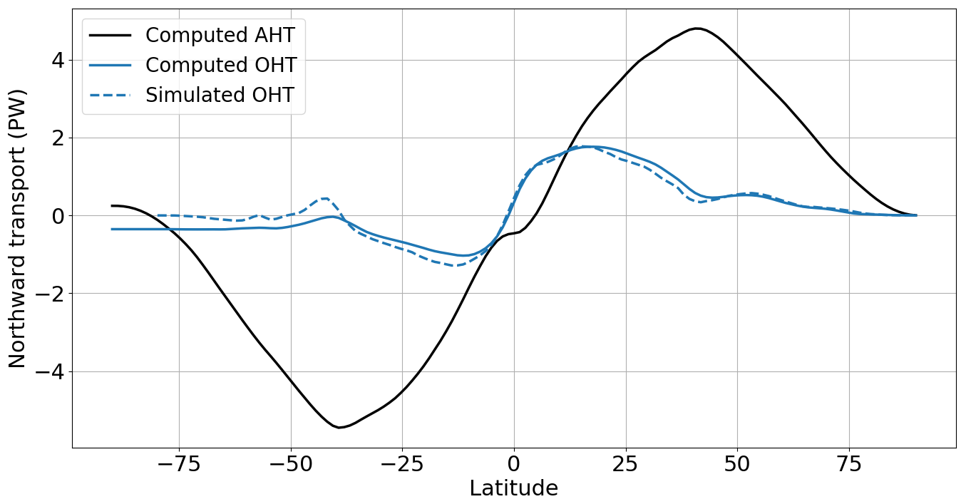
Figure 4 Annual zonal mean northward heat transport (PW) for the pre-industrial period. The northward heat transported computed as residual is represented by a solid line. The atmospheric heat transport is in black and the oceanic transport is in blue. The oceanic heat transport simulated by the IPSL-CM6A-LR model is represented by the dashed blue line.

The annual value of storage terms should be zero in the ideal case of an equilibrium climate. This is not the case for both simulations. The PI AHS and OHS are lower than the current observed energy imbalance of 0.5 W m⁻² in terms of absolute value (Roemmich et al., 2015; Hobbs et al., 2016). However, the LIG AHS and more specifically the LIG OHS are far above this reference value since they are, respectively, equal to 0.5 and 1.1 W m⁻². This “energy excess” may arise from assumptions made for the energy budget computation or from an ocean drift in the LIG simulation. Nevertheless, Fig. 5 shows that the SST and ocean heat content drifts are small over the last 200 years of the simulations.

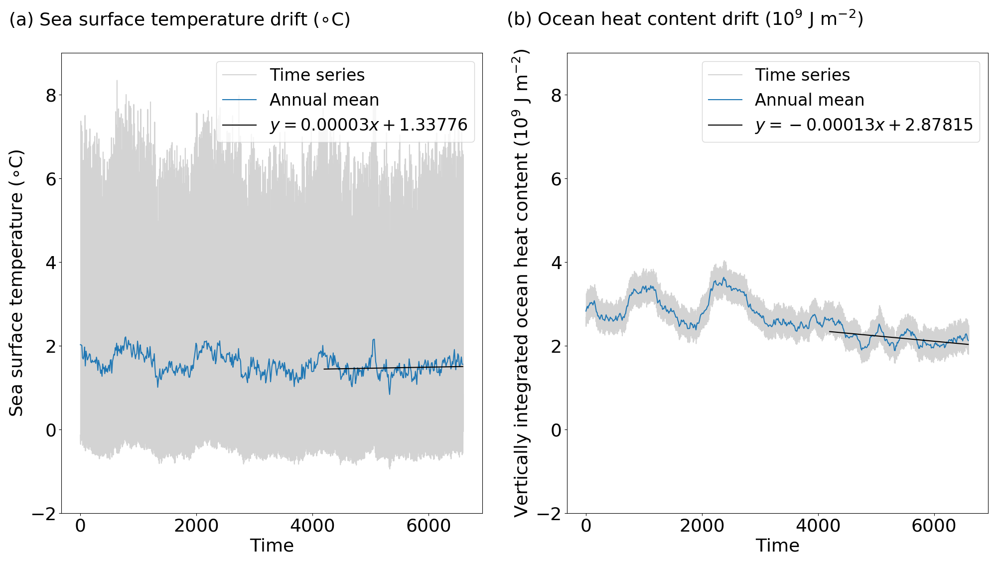
Figure 5 Time series of (a) the sea surface temperature (^∘C) and (b) the vertically integrated ocean heat content (J m⁻²) averaged over the Arctic region (60–90^∘ N) for the Last Interglacial. The time axis indicate the number of months since the year 1850.

We also estimate the energy provided by snowfall (E_SF, Eq. 14) as defined by Mayer et al. (2017, 2019):

$$\begin{array}{}\text{(14)}& E_{\mathrm{SF}}=L_{\mathrm{f}}\left(T_{\mathrm{p}}\right)P_{\mathrm{snow}},\end{array}$$

where L_f(T_p) is the latent heat of fusion ($-\mathrm{0.3337}\times {\mathrm{10}}^{\mathrm{6}}$ J kg⁻¹) and P_snow is the snowfall rate (in kg m⁻² s⁻¹).

We obtain an annual snowfall contribution to the atmospheric heat budget of 2.95 W m⁻² for the PI period and of 2.66 W m⁻² for the LIG period. The LIG–PI anomaly is very small compared to the anomaly of the other fluxes. Thus, we have decided to neglect the snowfall contribution in the rest of this study.

3 Results

In this section, we present anomalies defined as the difference between the simulated LIG and PI climatic fields.

3.1 Seasonal variations of the Arctic climate during the Last Interglacial period

Change in insolation between the LIG and the PI periods leads to an annual Arctic near-surface air temperature anomaly of 0.9 ^∘C. This value is in the range of the PMIP4 multi-model mean of 0.82±1.20 ^∘C (Otto-Bliesner et al., 2021). Furthermore, the IPSL-CM6A-LR model simulates cooler mean annual near-surface air temperatures than the maximum reconstructed value of 2^∘ (Turney and Jones, 2010; McKay et al., 2011; Capron et al., 2014). Indeed, despite the 127 ka period being near the peak warmth, it does not correspond to the warmest period of the Last Interglacial. Moreover, this mismatch can also be partly amplified by the use of prescribed ice sheets and vegetation, which results in ignoring the ice sheet–climate and vegetation–climate feedback (Otto-Bliesner et al., 2017).

The surface air temperature anomaly displays substantial seasonal (Fig. 6) and spatial variations (Fig. 7). During the LIG, winter (DJF) and spring (MAM) seasons are about 0.1 ^∘C colder compared to the PI period. Most of this cooling takes place over continents (Fig. 7a, b). Conversely, over the Arctic Ocean, the surface air temperature anomaly is positive, especially in areas where sea ice concentration decreases (Fig. 7a, b, e and f). This difference between land and ocean is explained by the larger effective heat capacity of the ocean resulting in a greater amount of energy absorbed and stored by the ocean. However, it should be noted that even if the seasonal averages of the surface air temperature anomalies is similar in winter and spring when averaged over the whole Arctic region, the magnitude of the anomalies is locally higher in winter.

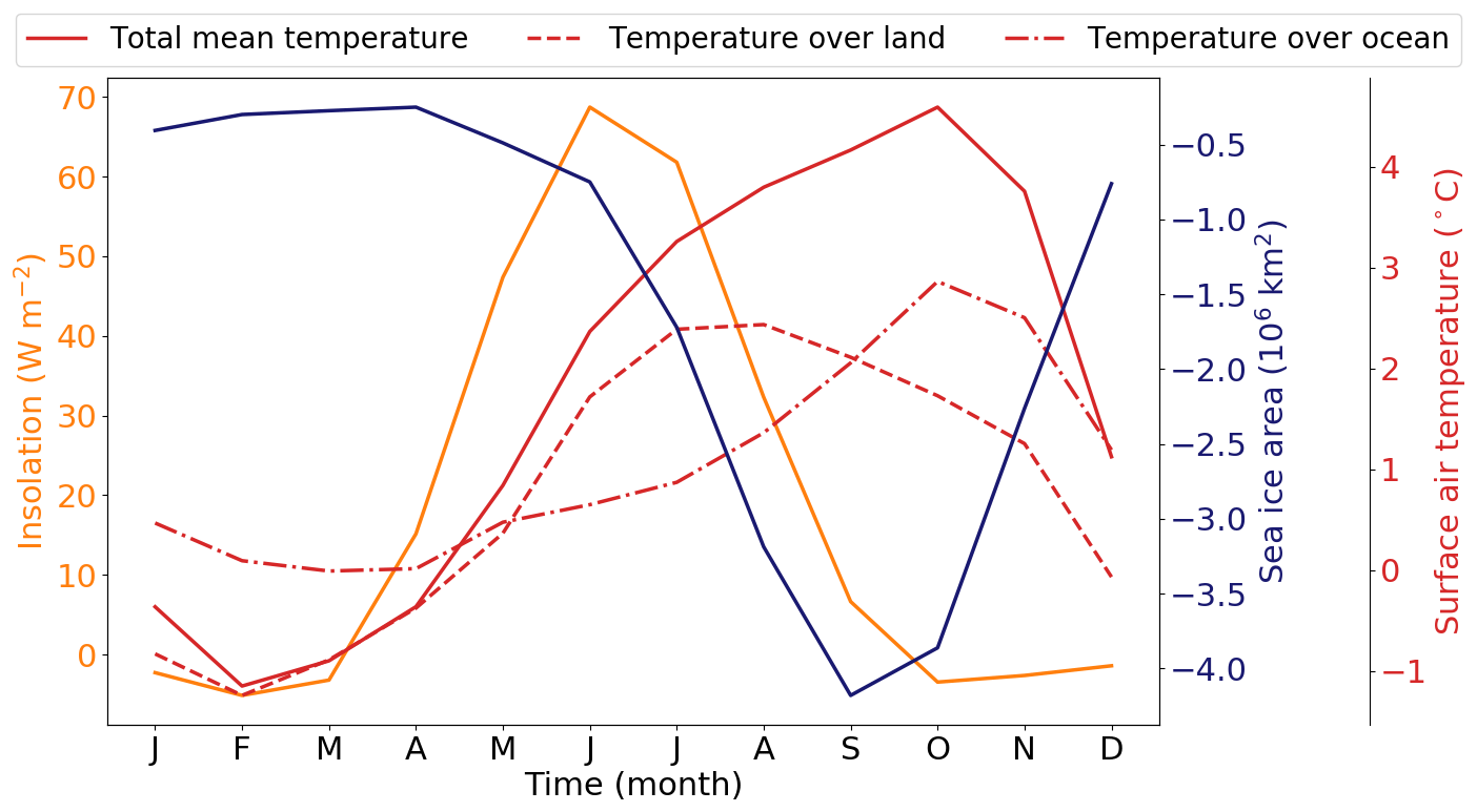
Figure 6 Annual cycles of solar radiation (orange line), surface air temperature (red lines) and sea ice area (dark blue line) LIG–PI anomalies. Variables are averaged between 60 and 90^∘ N.

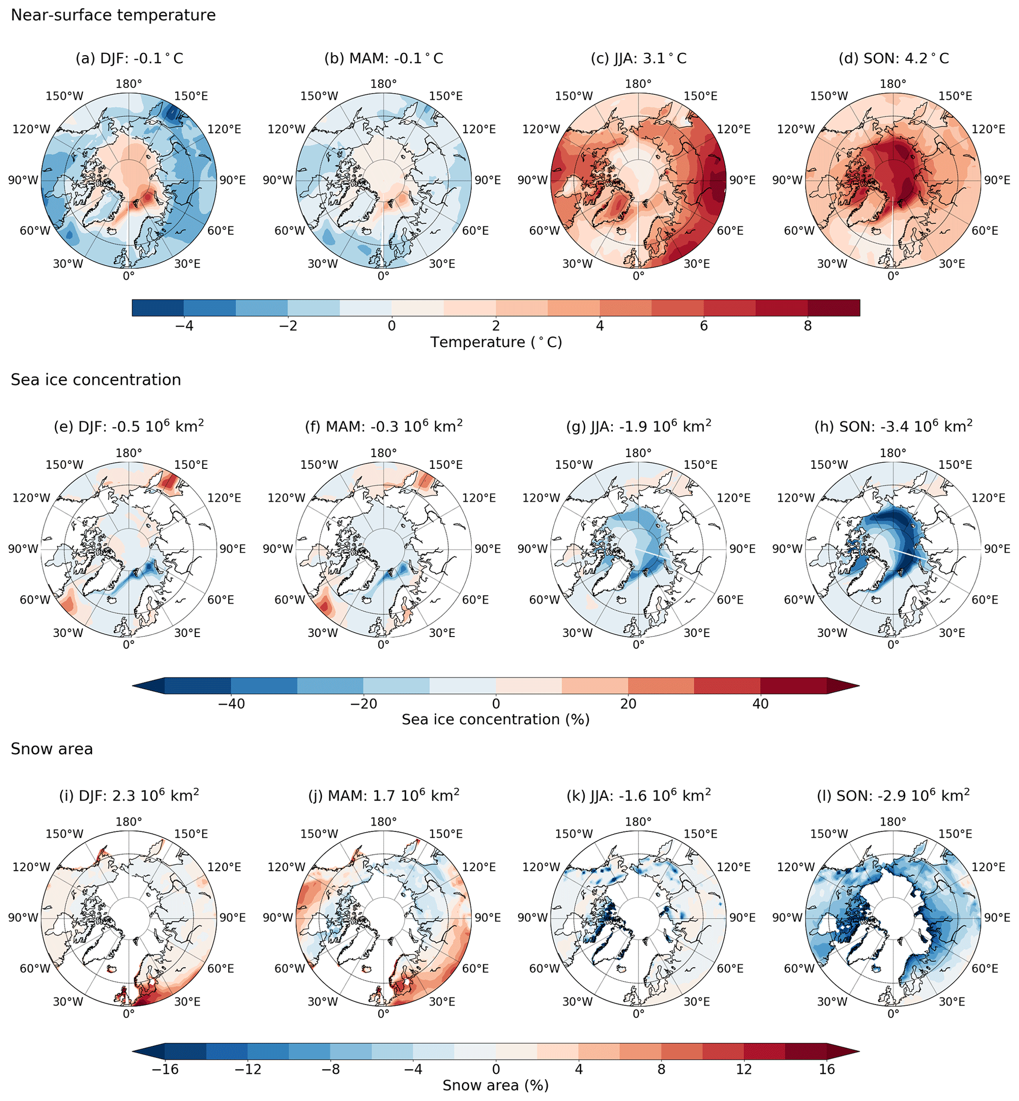
Figure 7 Seasonal cycles of the near-surface air temperature (a–d), sea ice concentration (e–h) and snow cover (i–l) LIG–PI anomalies. The value mentioned above the maps is the spatial average of the three variables over the Arctic region (60–90^∘ N). Seasons are abbreviated as follows: DJF is December–January–February (winter); MAM is March–April–May (spring); JJA is June–July–August (summer); SON is September–October–November (autumn).

Summer (JJA) and autumn (SON) are warmer during the LIG than during the PI period over both the ocean and the continents. The behaviour of the climatic fields is very different for both seasons. While the maximum warming occurs in summer over continental areas, over the oceanic regions, the largest temperature anomalies are found in autumn. There are also differences in the magnitude of summer and autumn warmings. The temperature anomaly is expected to be especially large in summer when the insolation anomaly is the largest. Indeed, it reaches +3.1 ^∘C on average over the Arctic region, but the autumn value is even larger and reaches +4.2 ^∘C (Figs. 6 and 7c, d).

Surface air temperature anomalies are also associated with variations of snow cover and Arctic sea ice. The strong warming occurring during summer and autumn results in a large retreat of the Arctic sea ice cover that persists during the rest of the year south of Svalbard and in the Barents Sea (Fig. 7e–h). On the other hand, the snow cover does not appear to respond to the temperature rise in summer (Fig. 7i–l). The snow cover anomaly is generally very low because the PI snow cover is relatively small during summertime. However, in autumn, the snow cover anomaly is strongly negative. The cooling in DJF and MAM reduces the effects of polar amplification in summer and autumn. Despite the slight decrease in temperature in DJF and MAM, sea ice does not fully recover after its strong decline during the summer and autumn seasons. As a result, compared to the PI simulation, the sea ice area decreases by 0.5×10⁶ km² in DJF and by 0.3×10⁶ km² in MAM.

Figure 6 displays a time lag of 4 months between the maximum of insolation (in June) and the surface air temperature (in October) anomalies. This lag has already been observed in previous studies investigating the future polar amplification (Manabe and Stouffer, 1980; Rind, 1987; Holland and Bitz, 2003; Lu and Cai, 2009; Kumar et al., 2010). It suggests the existence of processes limiting the summer warming and/or feedback inducing a strong warming in autumn despite the decrease in insolation anomaly. In the following, we investigate the origin of this time lag. To achieve this, we analyse the respective roles of the atmosphere, ocean, sea ice and continental surfaces in summer (Sect. 3.2) and in autumn (Sect. 3.3).

3.2 The Arctic summer warming

In summer, the positive anomaly of near-surface air temperature reaches 3.1 ^∘C over the Arctic and it is associated with a large retreat of the sea ice area of 1.9 million km² (see Sect. 3.1). As previously mentioned, this warming corresponds to a strong insolation anomaly in the high latitudes of the Northern Hemisphere. It affects the entire atmospheric column with a maximum air temperature anomaly between 600 and 300 hPa reaching more than 5 ^∘C (Fig. 8a). At the top of the atmosphere, downwelling shortwave radiation (SWdnTOA) increases by more than 25 W m⁻² on average compared to PI (Fig. 9). This energy excess is uniformly distributed between 60 and 90^∘ N. Since solar forcing only depends on latitude, it is similar over land and ocean. However, only 25 % of this energy excess is absorbed by the ocean and 50 % by the continents.

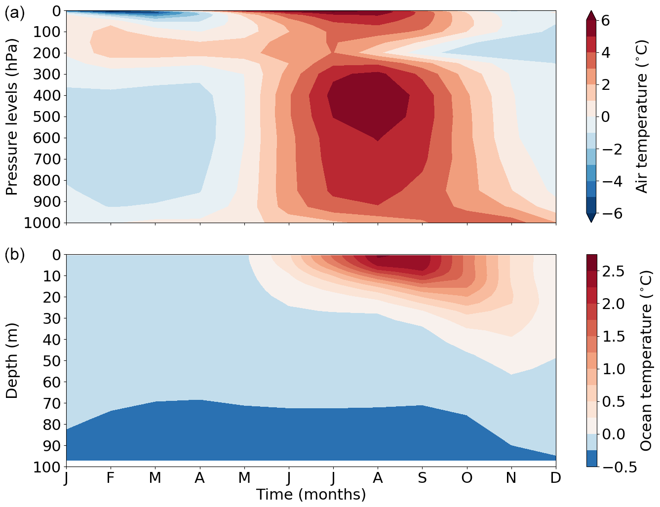
Figure 8 Annual evolution of LIG–PI temperature anomalies averaged over the Arctic region (60–90^∘ N), as a function of pressure in the atmosphere (a) and depth in the ocean (b). Below 100 m depth, the ocean temperature anomaly is negative and ranges between 0 and −0.53 ^∘C.

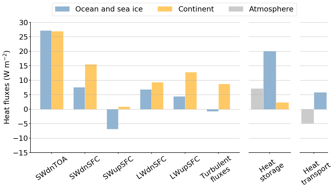
Figure 9 Quantification of the LIG–PI anomalies of the surface heat fluxes (left), storage terms (centre) and oceanic and atmospheric heat transport (right) for summer. Each flux included in the surface heat budget computation is plotted: solar radiation received at the surface (SWdnSFC), solar radiation reflected by the surface (SWupSFC), longwave radiation emitted by the surface (LWupSFC), longwave radiation emitted by the atmosphere (LWdnSFC) and turbulent fluxes given as the sum of latent and sensible heat fluxes. Variables are averaged between 60 and 90^∘ N. The surface heat flux anomalies are positive when the flux is stronger during the LIG.

3.2.1 Over the ocean

Over the ocean, a large amount of insolation anomaly does not reach the surface and is absorbed or reflected by the atmosphere. As aerosols are prescribed, this may be attributed to changes in the distribution or the characteristics of the cloud cover. Over the Arctic region, low-level clouds dominate (Shupe and Intrieri, 2004; Kay et al., 2016). They are often composed of both supercooled liquid water and ice. This type of cloud has a strong radiative effect on shortwave radiation, notably through the variations of the liquid water path, a measure of the weight of the liquid water droplets in the atmosphere above a unit surface area on the Earth (the American Meteorological Society (AMS) glossary). Figure 10a shows a small cloud cover anomaly over the Arctic Ocean but the liquid water path increases (Fig. 10d) causing more reflection of solar radiation back to space (see Sect. 1). As the LIG–PI liquid water path anomaly is very high (more than 2 g m⁻²) over the Arctic Ocean, the effect of cloud on incident shortwave radiation seems to be fundamental to explain the difference in energy received over the ocean and continents.

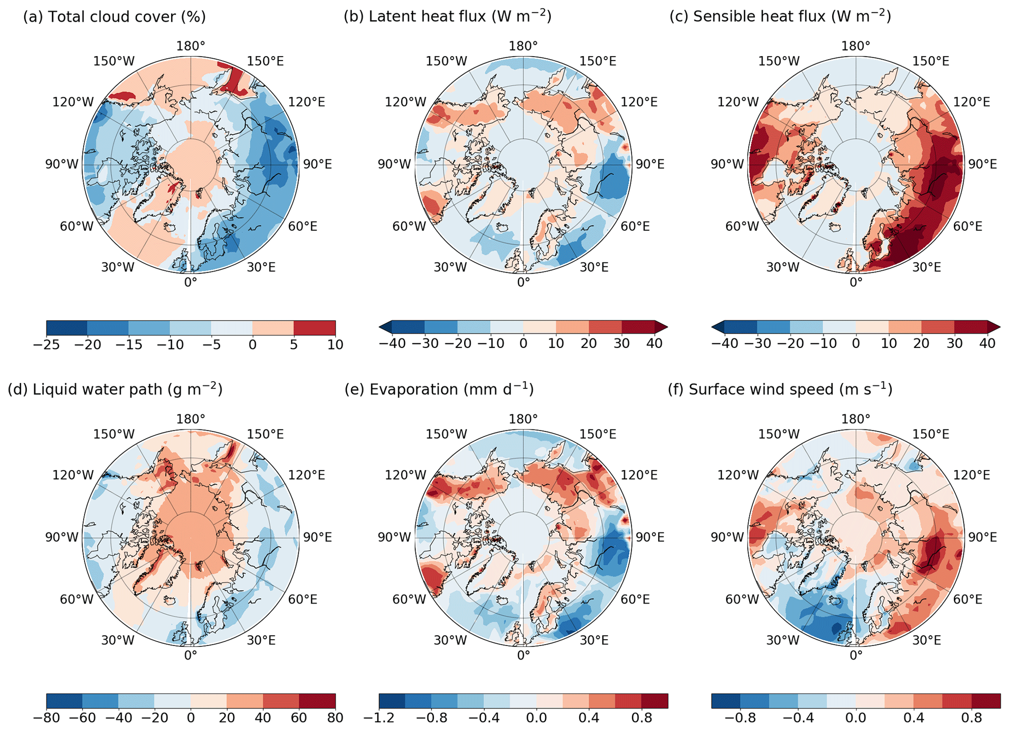
Figure 10 Summer LIG–PI anomalies of (a) total cloud cover (%), (b) latent heat flux (W m⁻²), (c) sensible heat flux (W m⁻²), (d) liquid water path (g m⁻²), (e) evaporation (mm d⁻¹) and (f) surface wind speed (m s⁻¹).

To better quantify the total impact of clouds on the Arctic shortwave budget, we compute the shortwave cloud radiative effect (SW CRE), defined as the difference in shortwave fluxes between an atmosphere with and without clouds. In both LIG and PI simulations, the SW CRE is negative over ocean (not shown), implying a strong cooling effect of clouds on the Arctic climate. The LIG SW CRE absolute value is about 31 % higher than the PI one on average (not shown). This leads to a negative SW CRE anomaly over the ocean in summer (Fig. 11a), which is consistent with the liquid water path anomaly (Fig. 10d).

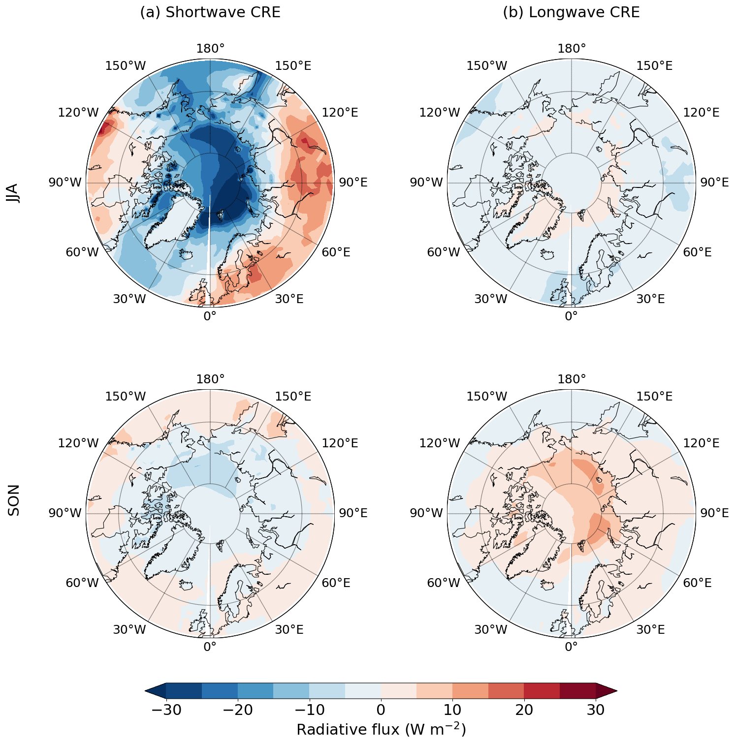
Figure 11 Summer (JJA) and autumn (SON) LIG–PI anomalies of (a) the shortwave cloud radiative effect (SW CRE) and (b) the longwave cloud radiative effect (LW CRE). All radiative fluxes are in W m⁻².

Despite a small incident solar radiation (SWdnSFC) anomaly over the ocean, surface heat flux anomalies are high enough to impact the sea ice cover (Fig. 7g). As sea ice declines, more oceanic surface is exposed and can interact with the atmosphere reducing the reflective power of the surface. Due to this albedo effect, the SWupSFC anomaly is negative over the ocean (Fig. 9) and more solar radiation is absorbed and stored in the upper layers of the ocean. This results in a warming of the oceanic surface and a large increase of the ocean heat storage (Fig. 9). According to the Planck's law, LWupSFC increases as a function of σT⁴. Consequently, ocean emits more longwave radiation compared to PI but the total longwave radiation (LWdnSFC–LWupSFC) anomaly is positive (Fig. 9) and strengthens the warming of the oceanic surface. Considering all the heat fluxes at the air–sea interface, the ocean receives 14.9 W m⁻² more energy than during the pre-industrial period. Turbulent heat fluxes show small variations, with a negative anomaly of −1.4 W m⁻² on average.

The surface heat budget over the ocean confirms that the upper layer of the ocean warms up during the LIG. Unlike the atmospheric warming that affects the entire atmospheric column, the increase in ocean temperatures only appears in the upper 100 m of the ocean (Fig. 8). This can be explained by the ocean stratification that limits the depth of seasonal heat exchange and mixing with the deepest oceanic layers. In addition, ocean heat transport (OHT) shows a significant anomalous heat convergence towards the high latitudes of the Northern Hemisphere. With a positive anomaly of more than 5 W m⁻² (Fig. 9), it represents an important source of heat. In the PI simulation, OHT is negative, which means that heat is advected away from the Arctic Basin to balance surface forcing (not shown). It becomes positive in the LIG simulation as surface heat flux also increases over the ocean (Eq. 13). This implies that ocean is affected by thermodynamic and/or dynamic changes.

Changes in heat transport, surface heat budget and, to a lesser extent, sea ice–ocean heat flux contribute to increase the ocean heat storage (OHS). The value of the oceanic heat storage nearly doubles compared to PI. This strong increase suggests that ocean is a key factor in the warming of the Arctic region in summer.

3.2.2 Over the continents

Over the continents, the positive SWdnSFC anomaly contributes to warm the surface and the lower atmosphere. This warming is amplified by a reduced negative shortwave CRE relative to the pre-industrial period (Fig. 11a). It is caused by a decrease in cloud cover and liquid water path over the continents relative to PI (Fig. 10a and d). Changes in cloud characteristics have an adverse effect on incident SW radiation over the continents and ocean, and thus they contribute to increase the land–ocean contrast in the near-surface air temperature anomaly.

The energy received at the surface is partly emitted back to the atmosphere through upwelling shortwave radiation (SWupSFC), upwelling longwave radiation (LWupSFC) and turbulent fluxes. The SWupSFC anomaly is very small relative to the other upward heat flux anomalies (Fig. 14) because of small changes in surface albedo associated with slight variations in summer snow cover. Due to the large SWdnSFC anomaly over the continents, temperatures rise significantly compared to PI leading to an LWupSFC anomaly of 12.8 W m⁻² (Fig. 9) partially compensated for by the positive LWdnSFC anomaly (9.3 W m⁻²). As the anomaly of the longwave CRE (Fig. 11b) is very weak, an increase in LWdnSFC is not related to changes in cloud cover. However, it could be caused by increasing specific humidity in the atmosphere (Fig. 12). A greater amount of water vapour leads to a larger absorption of longwave radiation, which amplifies the greenhouse effect and then the temperature.

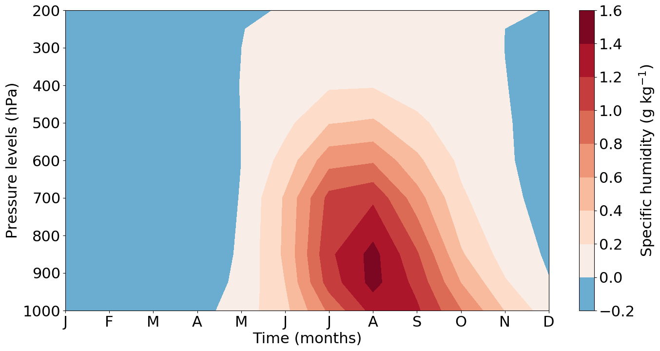
Figure 12 Annual evolution of the LIG–PI specific humidity anomaly (g kg⁻¹) according to pressure levels (hPa). The specific humidity anomaly is represented from the surface to 200 hPa and is spatially averaged over the Arctic region (60–90^∘ N).

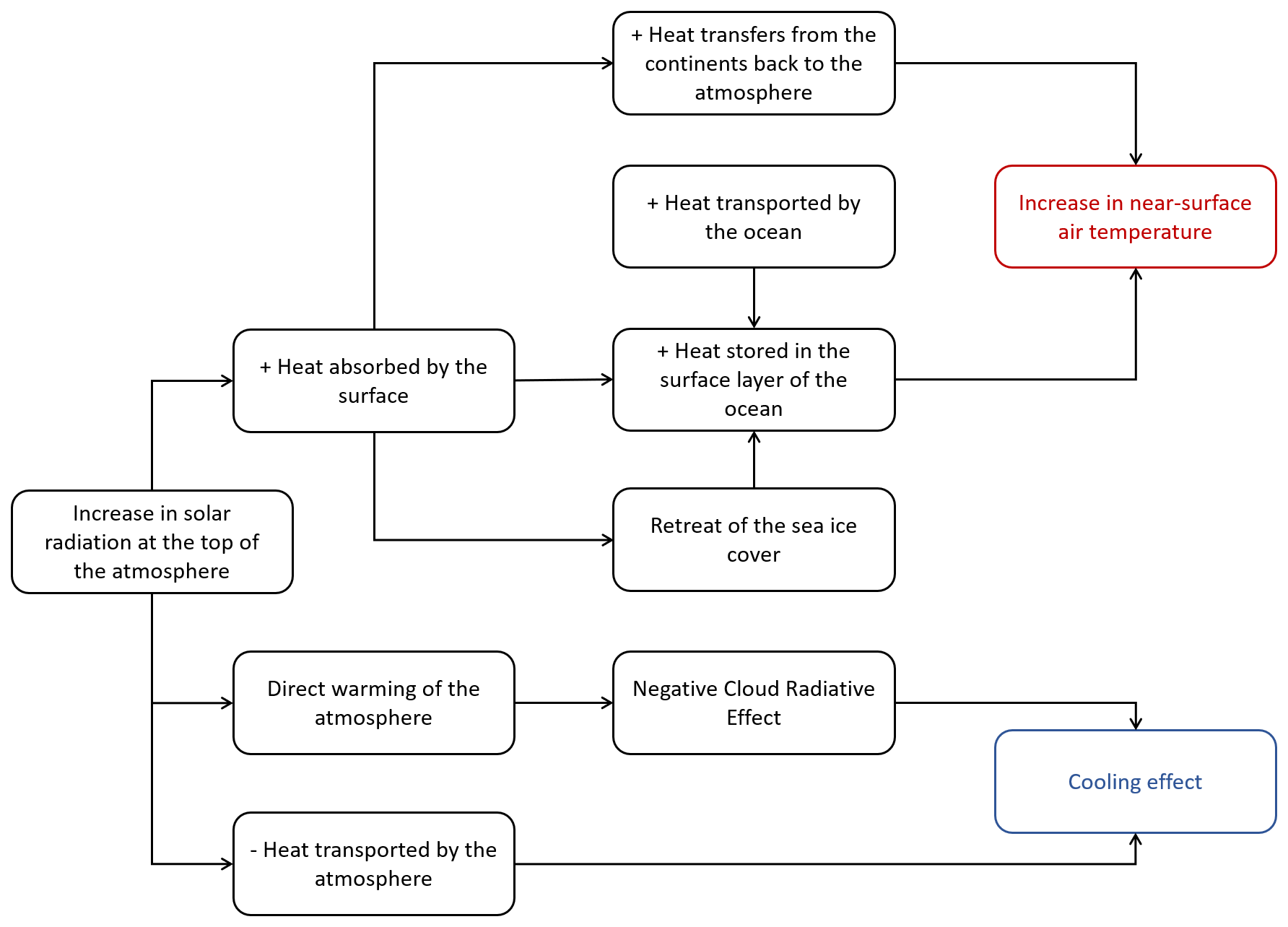
Figure 13 Diagram of the Last Interglacial climate processes and feedback involved in the Arctic summer warming.

Latent and sensible heat fluxes both contribute to the turbulent heat flux anomaly. Their respective contributions differ from one region to the other. Over Alaska, northeastern Canada, Siberia and Scandinavia, the latent heat flux anomaly is significant. It is not driven by snow sublimation as snow cover anomaly is very low, except in the Canadian archipelago (Fig. 7c).

Where latent heat flux anomaly is negative or approaches 0 W m⁻², there is an enhancement of the sensible heat flux. Turbulence is generated in the boundary layer as wind speed intensifies over land surface (Fig. 10c and f). However, changes in surface wind speed do not appear to amplify the latent heat flux. An explanation of this could be that, in regions with a strong positive anomaly of surface wind speed and a negative anomaly of latent heat flux, there is less water in the soil to evaporate.

The land energy budget confirms that continental surfaces lose energy to the benefit of the atmosphere. The shortwave radiation anomaly warms the continents, which in turn transfer the energy back to the atmosphere through longwave radiation (3.5 W m⁻²) and turbulent heat fluxes (8.7 W m⁻²).

The atmospheric heat storage (AHS) increases by 7.1 W m⁻² compared to PI. AHS depends on changes in the internal, latent, kinetic and potential energy storage anomalies (Eq. 2). Because of enhanced heat fluxes towards the atmosphere (SWdnTOA, LWupSFC and turbulent fluxes), the internal energy storage and, to a lesser extent, the latent and kinetic energy storage increase relative to PI, leading to a higher atmospheric energy storage during the LIG of 7.1 W m⁻² (Fig. 9). The AHS anomaly is lower than the OHS one mainly because of the much higher heat capacity of the ocean. Moreover, the atmospheric heat transport (AHT) does not contribute to the summer warming. Since it decreases from PI to LIG, the AHT anomaly almost balances the OHT anomaly. This strong negative relationship between changes in AHT and OHT was first suggested by Bjerknes (1964) and has been simulated by many modelling studies (see Swingedouw et al., 2009, for example). The AHT is partly reduced due to the decrease of the Northern Hemisphere meridional temperature gradient and thus the decrease of the poleward dry static energy transport.

In conclusion, the ocean and the continents respond in different ways to the orbital forcing in summer. While the oceanic surface tends to warm up as it better absorbs solar radiation, the continental surface provides energy back to the atmosphere. This result is in line with Bakker et al. (2014), who identified during the warmest months of the Last Interglacial near-surface air temperature changes over land 1.8 times larger than those over the adjacent ocean in the midlatitudes to high latitudes of the Northern Hemisphere.

The LIG summer warming is directly due to orbital forcing changes and heat exchange between the atmosphere and the continents surrounding the Arctic Ocean. Processes detailed in this section for the Arctic summer warming are summarised in Fig. 13.

3.3 The Arctic autumn warming

Despite a small insolation anomaly (Fig. 1), the strongest surface warming occurs in autumn (Fig. 7d). Figure 8 shows that the warming does not extend over the entire atmospheric column as in summer but is confined in the lower layers of the atmosphere below 800 hPa.

In autumn, the LIG insolation is similar to the PI one (Fig. 1). As a consequence, the shortwave radiation anomalies (SWdnTOA, SWdnSFC and SWupSFC) do not much contribute to the total energy budget anomaly compared to summer (Fig. 14 compared to Fig. 9). By contrast, longwave radiation anomalies play a crucial role in the autumn warming. Larger longwave fluxes are also emitted into the atmosphere because open ocean waters are warmer than the cold sea ice surface. The LWupSFC anomaly is 11 W m⁻² on average (Fig. 14) and peaks at more than 40 W m⁻² over the East Siberian and the Kara seas (Fig. 15d). Similarly to the summer months, the LWdnSFC anomaly is stronger than the LWupSFC anomaly resulting in a positive longwave radiative budget. The increase in specific humidity over the ocean (Fig. 12) is likely related to the large retreat of sea ice cover and associated evaporation (Figs. 7h and 15f). In response to increasing humidity in the atmosphere (Fig. 12), the Arctic cloud cover expands (Fig. 15c), leading to a positive cloud feedback over the Arctic Ocean (Fig. 11b). This longwave cloud radiative effect (LW CRE, computed in a similar way to the SW CRE) favours the autumn warming by trapping outgoing LW radiation in the atmosphere (Schweiger et al., 2008; Goosse et al., 2018).

Figure 14 Same as Fig. 9 for SON.

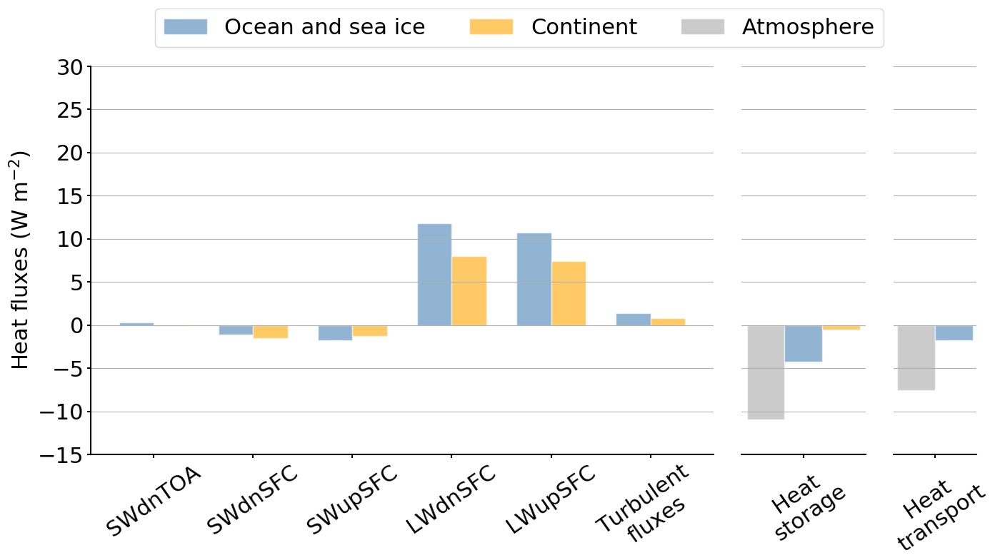
Figure 15 Autumn LIG–PI anomalies of (a) longwave radiation emitted by the atmosphere, (b) latent heat flux, (c) total cloud cover, (d) longwave radiation emitted by the surface, (e) sensible heat fluxes and (f) evaporation. All heat fluxes are in W m⁻², the total cloud cover in % and the evaporation in mm d⁻¹.

The surface air temperature anomaly and the additional heat absorbed by the upper ocean during summer amplify the retreat of the sea ice edge. The autumn months experience the largest sea ice decline with a sea ice area anomaly of $-\mathrm{3.5}\times {\mathrm{10}}^{\mathrm{6}}$ km² (Fig. 7h). This reveals large open-water areas which favour heat transfer from ocean to the atmosphere. Figure 14 indicates that turbulent heat fluxes slightly increase (by 1.9 W m⁻² on average over the ocean). However, at the local scale, their contribution is larger (Fig. 15b and e). In regions where the sea ice loss is the greatest (i.e. along the Siberian and Alaskan coasts and over the Barents and Greenland seas), the sum of sensible and latent heat fluxes reaches more than 20 W m⁻² (Fig. 7h). Over the continental areas, the turbulent heat fluxes anomaly does not seem to have a significant impact on the surface heat budget (Fig. 14).

Despite the strong Arctic warming, the atmospheric energy storage (AHS) anomaly is negative, meaning that the atmosphere loses more energy than it does for the PI period. During autumn, the internal energy storage (−4.9 W m⁻²) and the potential energy storage anomalies (−4.5 W m⁻²) contribute significantly to the energy loss (Table 2). The anomaly of the internal energy storage depends on air temperature fluctuations from one season to the other. As illustrated in Fig. 8, the air temperature increases from summer to autumn near the surface but peaks in August over the rest of the atmospheric column. The potential energy storage anomaly is also strongly dependent on the temperature in the atmospheric column and follows the same trend as the internal energy storage from summer to autumn.

Table 2 Seasonal anomalies of the atmospheric heat storage and its components (W m⁻²) averaged between 60 and 90^∘ N.

Moreover, poleward oceanic and atmospheric heat transport weakens (Fig. 14). This modulates the warming of the Northern Hemisphere high latitudes and does not contribute to the observed temperature increase.

Processes of the Arctic autumn warming are summarised in Fig. 16.

In summary, the Arctic region continues to experience the effects of the preceding summer warming through ocean and sea ice feedback during the autumn. Sea ice cover changes allow the ocean to release heat leading to a significant warming of the surface atmospheric layer. As illustrated in Fig. 8, feedback only operates in the lower atmosphere. Yin and Berger (2012) first explained such process using a surface heat budget analysis with the LOVECLIM-LLN model, which they called the “summer remnant effect”. This effect modifies the seasonal impact of the astronomical forcing. In the IPSL-CM6A-LR model, it appears during autumn and, to a lesser extent, persists until winter.

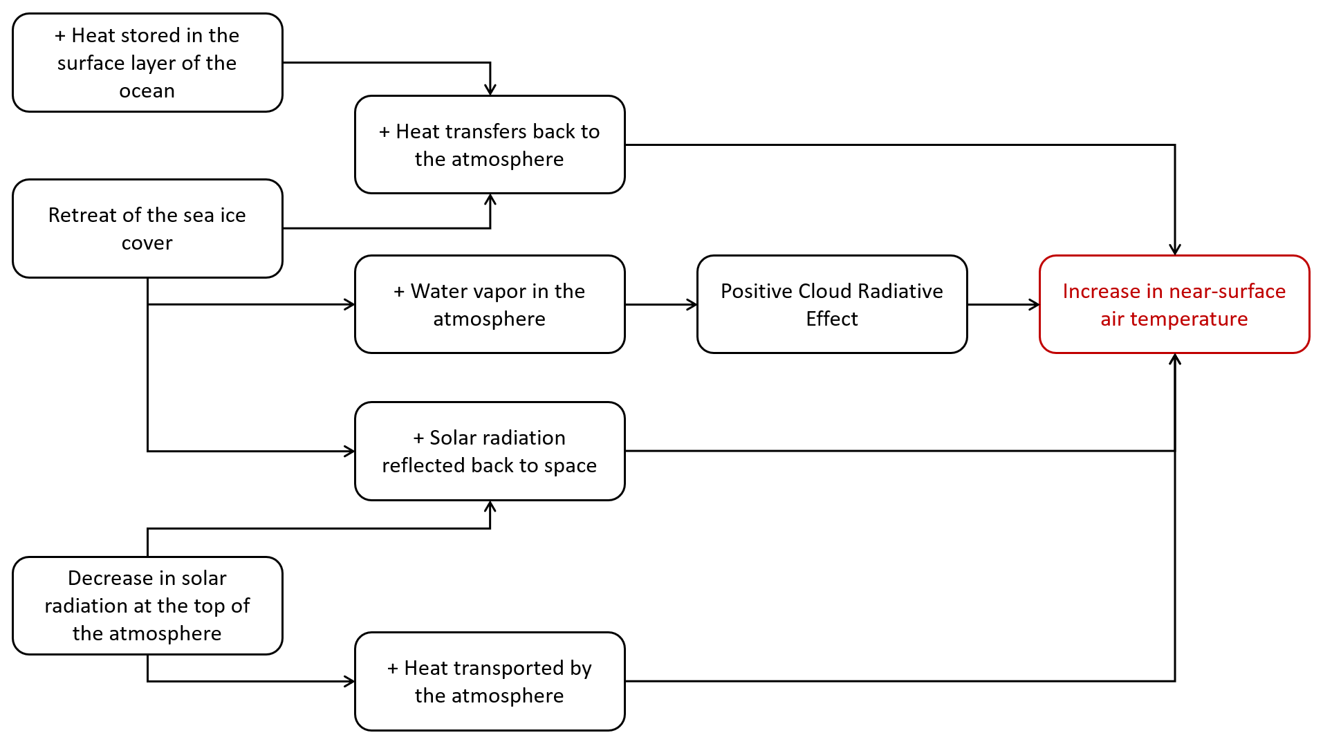
Figure 16 Diagram of the Last Interglacial climate processes and feedback involved in the Arctic autumn warming.

3.4 The Arctic sea ice mass variations

Section 3.2 and 3.3 highlight the key role of Arctic sea ice on the ocean and atmosphere heat balances. In particular, the expansion of sea ice cover determines the amplitude of air–sea exchange through variations of surface albedo and sea ice insulating effect. During the LIG, the sea ice cover is reduced all year round relative to the PI period, reaching a peak of $-\mathrm{3.4}\times {\mathrm{10}}^{\mathrm{6}}$ km² in autumn (Figs. 6 and 7e–h). The sea ice mass decreases too and loses about 0.08 Gt on annual average. To better understand the causes of this decline, we compute the anomalies of the different terms of the mass budget using new diagnostics developed for CMIP6 (Notz et al., 2016; Keen et al., 2021). These terms are the following: the basal growth, the ice formation in supercooled open water (or frazil), the melting at the top surface and the base of the ice, the ice formation due to the transformation of snow to sea ice, the change in ice mass due to evaporation and sublimation and the ice advection into or outside the Arctic domain. The IPSL-CM6A-LR model outputs do not contain explicit lateral melt. These different processes are represented in Fig. 17 in summer and autumn for both PI and LIG periods. In summer, the main process responsible for sea ice melt is basal melt during both periods. However, the LIG–PI surface melting anomaly is higher than the LIG–PI basal melting anomaly. Thus, changes in summer sea ice volume are mainly related to changes in incident shortwave radiation rather than changes in ocean–sea ice energy exchange. In autumn, ice melt and growth processes are less strong during the LIG. The large autumn sea ice retreat (Fig. 7h) is therefore not caused by increasing melt. It is the consequence of the substantial sea ice loss during the previous summer, exacerbated by the poor recovery of sea ice cover in autumn. While Keen et al. (2021) show that it is one of the main factors of the mass budget variations, it is worth mentioning that in our study, this process is surprisingly weak (Fig. 17).

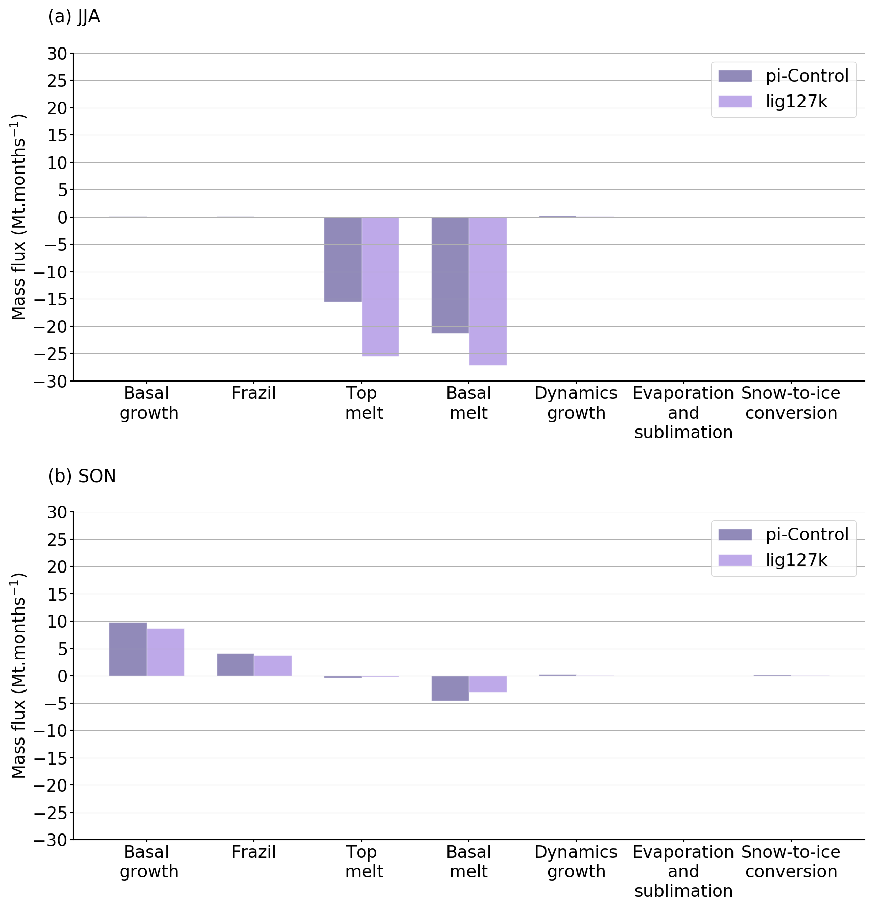
Figure 17 Components of the Arctic sea ice mass budget (Mt per month) in (a) JJA and (b) SON. They are computed for both the PI (dark purple) and LIG (pale purple) periods.

4 Discussion

As seen before, polar clouds greatly influence the cooling or the warming of the atmosphere. Despite their importance in the global energy budget, climate models have difficulties in representing the coexistence of supercooled liquid water and ice crystals in polar clouds, the fraction of the former being often underestimated. Regarding the IPSL model, improvements in shallow convective scheme and phase partitioning in mixed phase clouds between LMDZ5A and LMDZ6A lead to an increase of supercooled droplets and a better distribution between low-level and mid-level clouds, which is more consistent with the most recent satellite observations (Madeleine et al., 2020). These improvements, as well as a refined model tuning (Hourdin et al., 2020), result in a reduction of shortwave and longwave cloud radiative effects (CREs) in the mid- to high-latitude regions in good agreement with the observations. However, while the distribution of liquid droplets and ice crystals in cold mixed phase clouds is closer to observations, low-level clouds remain too abundant over high-latitude regions. The increase in low-level clouds seems to be compensated for by the decrease in the mid- to high-level clouds and finally does not impact the LW CRE.

As shown in Kageyama et al. (2021), while the insolation received at the top of the atmosphere is similar for all models following the PMIP4 lig127k protocol, the amplitude of the anomaly of the annual cycle of the downwelling shortwave radiation varies across PMIP4 models. The atmospheric energy budget can be analysed only for eight models (out of the initial 17 models) for which data were available. Even with this reduced dataset, the diversity of responses suggests that cloud feedback is not consistent in these climate models.

On the other hand, the temperature biases described in Sect. 2.2 can largely impact the surface heat budget, either directly through biases in longwave fluxes emitted by the Earth's surface or indirectly through changes in sea ice. The warm bias over the Arctic Ocean favours the retreat of the sea ice edge, which is highly sensitive to surface temperature changes. In their evaluation of the IPSL-CM6A-LR model, Boucher et al. (2020) compare sea ice area and extent in the historical simulations (1850–2014) with recent satellite observations. For both summer and winter, Arctic sea ice simulated by the model is slightly underestimated compared to satellite data but is still within observational uncertainty. During the LIG, this bias only subsists in summer especially in the northernmost areas (Kageyama et al., 2021). In winter, model and observations are in better agreement except for two sites in the Labrador Sea. At these locations, the model shows seasonal or perennial sea ice, while marine sediment cores provide evidence of ice-free conditions all year round (Kageyama et al., 2021).

On the basis of a simple linear regression model, we try to identify the relationship between surface temperature biases in the historical and the lig127k simulations. The aim is to determine if the model biases found in Boucher et al. (2020) are correlated with those of the lig127k simulation. Surface temperature biases are analysed at the core site location (Fig. 2). As in Boucher et al. (2020), near-surface air temperatures simulated by the historical simulation are compared with ERA-Interim dataset for the period 1980–2009 (Dee et al., 2011) and sea surface temperature with WOA13-v2 dataset for the period 1975–2004 (Locarnini et al., 2013). For the annual average, the lack of data points limits the interpretation of the linear regression and we cannot conclude on the impact of the model biases in the lig127k simulation (Fig. 18). For the summer average, the correlation coefficient is low (r²=0.18), which indicates that the model biases have only a limited influence on the lig127k. This result depends largely on the uncertainties of the reconstructions, which can be very large for some points. The uncertainty associated with the surface temperature biases during the Last Interglacial is plotted in Fig. 2. It is estimated from the data uncertainty (±1σ) and the standard deviation of the model outputs computed following a Gaussian distribution. Even though the correlation coefficient is low, Fig. 18b shows that the signs of the biases for the present day and LIG are generally consistent: there are only two sites for which the present bias is positive while the LIG bias is clearly negative, taking the uncertainties on the LIG reconstructions into account. This finding calls for further investigation in a forthcoming study.

Figure 18 Linear regression of surface temperature biases in the historical simulation versus surface temperature biases in the lig127k simulation. Blue circle markers represent the model biases at LIG terrestrial and marine ice core sites. The coefficient of correlation (r²) is calculated for each regression line. To compute model biases for the historical simulation, we use ERA-Interim near-surface air temperature data (1980–2005), the WOA13-v2 ocean temperature data (1985–2004) and the first member of the IPSL-CM6A-LR historical simulations. The error bars are plotted in blue and represent the uncertainty on the surface temperature biases during the Last Interglacial.

Otto-Bliesner et al. (2021) have highlighted the large differences in the magnitude of high-latitude near-surface temperature anomalies among PMIP4 climate models that have run the lig127k simulation. On an annual scale, Arctic near-surface temperature changes range from −0.39 to 3.88 ^∘C. Models simulating the most intense surface warming also show the largest reductions in minimum Arctic sea ice area (Kageyama et al., 2021; Otto-Bliesner et al., 2021). There is a large spread across models for the simulated summer Arctic sea ice area, with minimum sea ice area anomalies ranging from 0.22 to 7.47×10⁶ km² for the Last Interglacial. Moreover, there is no consensus about the sign of winter sea ice area variations, with three models simulating a decrease in sea ice area during this season.

Furthermore, the effective climate sensitivity (ECS) of PMIP4 models varies from 1.8 to 5.6 ^∘C (Otto-Bliesner et al., 2021). The IPSL-CM6A-LR model is in the higher range with an ECS value of 4.6 ^∘C. However, this model does not simulate a strong annual Arctic warming and a large summer Arctic sea ice retreat compared to other models with high ECS values such as EC-Earth3-LR (4.2 ^∘C) or HadGEM3 (5.6 ^∘C).

5 Conclusions and perspectives

In this work, we present an analysis of the seasonal cycle of the Arctic energy budget during the Last Interglacial period using IPSL-CM6A-LR model outputs.

In autumn, the near-surface air temperature anomalies are higher than in summer: there is a time lag between the maximum anomaly of temperature (October) and the maximum anomaly of insolation (June). The summer warming is directly linked to the insolation anomaly and thus to the anomaly in shortwave radiation received at the surface. Surface air temperature anomaly is higher over the continents. Continental surfaces absorb more solar radiation and release more heat back to the atmosphere through longwave radiation and turbulent fluxes. The warming persists in autumn as a result of different feedback involving ocean and sea ice. The Arctic Ocean and marginal seas, which play the role of a heat sink in summer, release heat back to the atmosphere. This effect is amplified by the sea ice edge retreat and by the water vapour feedback. Anomalies of sea ice cover and sea ice mass are negative throughout the year. The maximum ice loss is observed in the marginal seas in autumn. It is the result of increasing basal melt in summer and decreasing basal growth in autumn compared to PI.

Our simulations do not account for climate–vegetation and climate–ice sheet feedback, as vegetation and ice sheets are prescribed in IPSL-CM6A-LR piControl and lig127k simulations. Changing land cover would modify both the shortwave and longwave radiative budgets. Pollen and macrofossil data for the LIG indicate that boreal forests extended northward and replaced Arctic tundra (CAPE-Last Interglacial Project Members, 2006; Schurgers et al., 2007; Swann et al., 2010). The expansion of trees caused a decrease in surface albedo during the Last Interglacial by partly masking snow and enhancing water vapour release to the atmosphere through evapotranspiration. Therefore, additional simulation would be necessary to quantify the vegetation feedback on the energy budget. On the other hand, variations of the Last Interglacial Greenland ice sheet geometry compared to the PI one likely modified the radiative budget through the albedo and elevation feedback. Moreover, it may have altered the sea surface conditions and the oceanic circulation through freshwater release. Govin et al. (2012), Capron et al. (2014) and Stone et al. (2016) have shown that freshwater inputs to the North Atlantic from the Greenland ice sheet mass loss improve model simulations with respect to sediment and ice core data. However, accounting for the evolution of the Greenland ice sheet was not included in the PMIP4-CMIP6 protocol of the lig127k simulation followed here.

Investigating the energy budget of other PMIP4-CMIP6 lig127k simulations would allow to evaluate whether their temperature response to lig127k forcings is related to the same processes in terms of energy budget and to compare the strengths of these processes, especially in models which simulate a near-complete loss of Arctic sea ice in summer (Kageyama et al., 2021).