the Creative Commons Attribution 4.0 License.
the Creative Commons Attribution 4.0 License.
 | 16 Mar 2022
Marine carbon cycle response to a warmer Southern Ocean: the case of the last interglacial
Dipayan Choudhury
Laurie Menviel
Katrin J. Meissner
Nicholas K. H. Yeung
Matthew Chamberlain
Tilo Ziehn
Recent studies investigating future warming scenarios have shown that the ocean carbon sink will weaken over the coming century due to ocean warming and changes in oceanic circulation. However, significant uncertainties remain regarding the magnitude of the oceanic carbon cycle response to warming. Here, we investigate the Southern Ocean's (SO, south of 40∘ S) carbon cycle response to warmer conditions, as simulated under last interglacial boundary conditions (LIG, 129–115 ka). We find a ∼150 % increase in carbon dioxide (CO2) outgassing over the SO at the LIG compared to pre-industrial conditions (PI), due to a 0.5 ∘C increase in SO sea surface temperatures. This is partly compensated for by an equatorward shift of the Southern Hemisphere (SH) westerlies and weaker Antarctic Bottom Water formation, which both lead to an increase in dissolved inorganic carbon (DIC) in the deep ocean at the LIG compared to PI. These deep-ocean DIC changes arise from increased deep- and bottom-water residence times and higher remineralization rates due to higher temperatures. While our LIG simulation features a large reduction in SO sea ice compared to the PI, we find that changes in sea ice extent exert a minor control on the marine carbon cycle. The projected future strengthening and poleward shift of the SH westerlies coupled to warmer conditions at the surface of the SO should thus weaken the capacity of the SO to absorb anthropogenic CO2 over the coming century.
- Article
(11818 KB) - Full-text XML
- BibTeX
- EndNote


Future increases in atmospheric carbon dioxide (CO2) concentration are unequivocally projected to further warm the Southern Ocean (SO) and reduce sea ice concentrations (Bracegirdle et al., 2020). The current state of knowledge suggests the mitigating effects of carbon cycle feedbacks on global warming to be less efficient under future scenarios (Pachauri et al., 2014). This primarily stems from the changes in carbon uptake by the terrestrial biosphere and ocean under a changing climate. Both land and ocean presently act as sinks of anthropogenic carbon, each absorbing about 25 % of anthropogenic emissions (Friedlingstein et al., 2020), with 40 % of the ocean sink being attributed to the SO (Caldeira and Duffy, 2000; DeVries, 2014). The SO CO2 uptake weakened during the 1990s due to a strengthening and poleward shift of the Southern Hemisphere (SH) mid-latitude westerlies (Lovenduski et al., 2007; Le Quéré et al., 2007; Zickfeld et al., 2007; Gruber et al., 2019a, b) but strengthened in the 2000s due to cooling over the Pacific and increased stratification over the Atlantic and Indian sectors of the SO (Landschuetzer et al., 2016; Gruber et al., 2019b).
In addition, the consensus amongst studies analysing future climate simulations points towards amplified warming over high latitudes (Holland and Bitz, 2003; Smith et al., 2019; Fan et al., 2020). For example, the SO annual mean sea surface temperature (SST) anomaly is projected to exceed 0.5 ∘C for Shared Socioeconomic Pathway scenario (SSP) 245 and 1.5 ∘C for SSP 585 at 2100 relative to 2015 (Bracegirdle et al., 2020; Tonelli et al., 2021), with reduced sea ice during austral spring (Roach et al., 2020). At the same time, SH westerlies are projected to strengthen and shift poleward over the coming century (Collins et al., 2013; Zheng et al., 2013; Goyal et al., 2021). Overall, climate change will reduce the amount of anthropogenic carbon taken up by the ocean (Plattner et al., 2001; Bernardello et al., 2014; Wang et al., 2014; Howes et al., 2015) by reducing CO2 solubility (Bernardello et al., 2014), weakening the efficiency of the biological pump (Boyd, 2015), increasing outgassing from upwelling of Circumpolar Deep Waters (CDW) due to stronger and poleward-shifted SH westerlies (Lovenduski et al., 2007; Zheng et al., 2013; Gruber et al., 2019a), and reducing sea ice extent (Shadwick et al., 2021). However, uncertainties still remain in regards to the response of the SO carbon cycle under a warmer climate.
The last interglacial (LIG, 129–115 ka) was the warmest interglacial of the last 800 000 years (Masson-Delmotte et al., 2013; PAGES, 2016). The warmer climate at the LIG is primarily attributed to a stronger Northern Hemisphere summer insolation (Laskar et al., 2004) owing to the orbital configuration of higher eccentricity and obliquity (Berger, 1978), rather than higher greenhouse gas concentrations as projected for the future. The role of orbital forcing versus greenhouse gases on temperature has been analysed in detail in Yin and Berger (2012). The LIG is associated with annual mean SSTs around 0.5 ∘C higher than pre-industrial conditions (PI) (Capron et al., 2014; Hoffman et al., 2017), and sea level was ∼ 5 m higher than PI, with estimates ranging from 1.2 to 9 m higher (Dutton et al., 2015; Rohling et al., 2019; Dyer et al., 2021). The area-weighted summer warming is estimated to be 1.1–1.9 ∘C for the North Atlantic and 1.6–1.8 ∘C for the SO compared to PI (Govin et al., 2012; Capron et al., 2014; Hoffman et al., 2017). Summers over land areas are reconstructed to be 4–5 ∘C warmer at high latitudes in the Northern Hemisphere (CAPE-Last Interglacial Project Members, 2006), 3–11 ∘C over Greenland (Dahl-Jensen et al., 2013), and 2.2 ∘C over Antarctica (Masson-Delmotte et al., 2013). Reconstructions of sea ice are mostly focused on the Arctic and suggest ice-free conditions south of 78∘ N (Van Nieuwenhove et al., 2008, 2011, 2013; Kageyama et al., 2021). The Atlantic Meridional Overturning Circulation (AMOC) has been suggested to have weakened at the peak of the LIG (127 ka) and strengthened afterwards (Galaasen et al., 2014), with strong evidence pointing towards periods of reduced Antarctic Bottom Water (AABW) formation during the early part of the LIG due to discharges from the Antarctic ice sheet (Hayes et al., 2014; Rohling et al., 2019).
A few studies have investigated the terrestrial carbon response to LIG conditions (Kleinen et al., 2015; Brovkin et al., 2016), but the marine carbon cycle response at the LIG, and particularly in the SO, has received little attention. A comprehensive study of the changes in the SO carbon cycle at the LIG compared to PI can enhance our understanding of the processes involved in the SO carbon cycle and their sensitivity to changes in boundary conditions. It can also help us, to a certain extent, to better quantify the impact of expected future physical and dynamical changes in a warming SO on the marine carbon cycle, bearing in mind that there was no additional anthropogenic carbon released during the LIG.
Here, we study the impact of a warmer climate, in particular at high latitudes, on the oceanic carbon cycle by analysing an equilibrium last interglacial simulation (lig127k, Otto-Bliesner et al., 2017) performed with the ACCESS-ESM1.5 model (Ziehn et al., 2020; Yeung et al., 2021). The paper is structured as follows. In Sect. 2, components of the ACCESS-ESM1.5 model are described, followed by a framework for decomposing variables relevant for carbon cycle changes. The main results are presented in Sect. 3, discussing the changes in climate and the carbon cycle. These include differences in ocean properties, such as temperature, sea ice cover, stratification and circulation, and their effects on the carbon cycle, including air–sea fluxes, net carbon storage, and the efficiency of the biological pump. Finally, in Sect. 4, we conclude and discuss the limitations of the current study, including possible sources of uncertainty, and what inferences can be drawn for future global warming scenarios.
2.1 Model description and experimental design
An equilibrium last interglacial simulation (lig127k) is performed with the Australian Community Climate and Earth System Simulator Earth System Model, ACCESS-ESM1.5 (Ziehn et al., 2020), which includes interactive land and ocean carbon cycles and is Australia's submission to the Paleoclimate Modeling Intercomparison Project 4 (PMIP4) – Coupled Model Intercomparison Project (CMIP6) (Yeung et al., 2021). ACCESS-ESM1.5 differs from the previous version, ACCESS-ESM1 (Law et al., 2017) mostly in the land and ocean components. ACCESS-ESM1.5 is built upon the ACCESS1.4 physical model and includes the UK Met Office Unified Model (UM) version 7.3 (Martin et al., 2010; The HadGEM2 Development Team, 2011) as an atmospheric component, which is directly coupled to the updated land Community Atmosphere Biosphere Land Exchange model (CABLE) version 2.4 (Kowalczyk et al., 2013), both with a horizontal resolution of 1.875∘ × 1.25∘. UM has 38 vertical levels. The ocean model is the NOAA/GFDL Modular Ocean Model (MOM) version 5 (Griffies, 2014), which is coupled to the Los Alamos National Laboratory sea ice model (LANL CICE) version 4.1 (Hunke et al., 2010). MOM5's resolution is 1∘ × 1∘ with 50 vertical levels. The coupler is the Ocean Atmosphere Sea Ice Soil – Model Coupling Toolkit (OASIS-MCT) (Craig et al., 2017). The current version of the land model CABLE also includes biogeochemistry (BGC) implemented using the CASA-CNP module (Wang et al., 2010). The ocean carbon cycle is simulated using the Whole Ocean Model of Biogeochemistry And Trophic-dynamics (WOMBAT) model (Oke et al., 2013).
WOMBAT is a nutrient–phytoplankton–zooplankton–detritus (NPZD) model, with one class of phytoplankton and one class of zooplankton. It includes dissolved inorganic carbon (DIC), alkalinity (ALK), phosphate (PO4), oxygen (O2), and iron. The biogeochemical tracers are coupled using the stoichiometric C (carbon):N (nitrogen):P (phosphorous):O2 ratio of . The air–sea gas exchange is based on the square of the wind speed (Wanninkhof, 1992), and the seawater partial pressure of CO2 (pCO2) is calculated following the third phase of the Ocean Carbon-Cycle Model Intercomparison Project (OCMIP) protocol using temperature, salinity, DIC, ALK, and PO4. WOMBAT simulates production in and export from the photic zone and remineralization and dissolution at depth for both organic and inorganic (CaCO3) particulate matter, with parameters adjusted for inorganic export to be ∼8 % of organic export. The remineralization of organic matter is calculated based on depth- and temperature-dependent parameters, while the dissolution of CaCO3 uses a constant dissolution rate. ACCESS-ESM1.5 does not include a sediment component, and all particulates reaching the bottom ocean layer are instantly remineralized following the relevant remineralization rates. Other specific details of the model can be found in Oke et al. (2013), Law et al. (2017), and Ziehn et al. (2020).
A pre-industrial 1850 simulation (piControl) is run in accordance with the CMIP6 protocol (Eyring et al., 2016), with a constant atmospheric CO2 forcing of 284.3 ppm but using CMIP5 solar irradiance (1365.65 Wm−2, as explained in Ziehn et al., 2020). This simulation is run for 1000 years. Initialized from this PI control run, a LIG simulation (lig127k) is performed using orbital parameters following the PMIP4 protocol (Otto-Bliesner et al., 2017; Yeung et al., 2021) but with the solar constant adjusted to the CMIP5–PMIP3 value to be comparable to the piControl simulation (1365.65 Wm−2). CO2 concentration for the LIG is set at 275 ppm. Vegetation is kept constant at 1850 PI levels. The lig127k experiment is run for 650 years. The run is at equilibrium over the SO, although there is a small drift in globally averaged DIC of ∼1 µmol kg−1/100 yr−1 below 3 km. The analysis presented here is based on the average of the last 100 years of the lig127k simulation compared to the last 100 years of the piControl simulation. Further details on these experiments can be found in Otto-Bliesner et al. (2017), Ziehn et al. (2020), and Yeung et al. (2021).
WOMBAT includes two DIC tracers, one being forced by the prescribed atmospheric CO2 concentration (PI: 284.3 ppm; LIG: 275 ppm), and the other forced by a constant atmospheric CO2 concentration of 280 ppm. Unless otherwise stated, all of the analyses presented here are based on the tracers forced with CO2 concentrations of 280 ppm, while the climate response is forced with the radiative forcing of 284.3 ppm for PI and 275 ppm for the LIG. This allows quantification of the effects of the LIG climate on the carbon cycle independently of the difference in background CO2 concentrations.
2.1.1 Model evaluation
After a 3000-year and 1000-year spin up of the physical and biogeochemical states, a 500-year piControl run was generated and used to assess the performances of the ACCESS-ESM1.5. The drifts in the piControl simulation are described in Ziehn et al. (2020) and are ∘C century−1 for SST, 5.3 × 10⁻³∘C per century for global ocean temperatures, 7.6 × 10⁻⁴ psu per century for sea surface salinity (SSS), and 8.8 × 10⁻⁴ psu per century for global ocean salinity. The drift in total ocean productivity is −0.0163 PgC yr−1 per century and that in carbon flux is −0.0048 PgC yr−1 per century. The net pre-industrial carbon flux is 0.02 and 0.08 PgC yr−1 for land and ocean, respectively.
Ziehn et al. (2020) present results from the historical simulation performed with the ACCESS-ESM1.5 and evaluate the performance with respect to available observations. Here, we summarize the model performance pertaining to the SO. The model has a warm SST bias in the SO, possibly resulting from a too shallow and warm summer mixed layer; however, the climatological sea ice extent in the SO closely follows the observations (Fetterer et al., 2017). The ACCESS-ESM1.5 captures the surface patterns of nutrients relatively well, showing a 0.89 correlation with the surface phosphate distribution from World Ocean Atlas (Garcia et al., 2010b). The simulated primary productivity is higher over 40–45 ∘S compared to observations (Behrenfeld and Falkowski, 1997), which leads to an increased uptake of CO2 compared to the observed estimates (Takahashi et al., 2009). Compared to the GLODAP dataset (Key et al., 2004), phosphate and alkalinity concentrations are underestimated in the Southern Ocean by ∼0.4–0.8 and ∼50–100 mmol m−3, respectively. In addition, the oxygen concentration is ∼50–100 mmol m−3 higher in the ACCESS-ESM1.5 across all depths (Garcia et al., 2010a). These biases could result from a strong ocean ventilation or a weak biological pump in the SO. Further details on model performance and evaluation can be found in Ziehn et al. (2020).
2.2 pCO2 decomposition
Changes in surface pCO2, which ultimately control the direction and magnitude of air–sea fluxes, can further be decomposed into contributions from SST, SSS, DIC, and ALK (Sarmiento and Gruber, 2006). The SST contribution is calculated as
where represents the contribution of SST change to surface pCO2 change and γSST=0.0423 ∘C−1 is the sensitivity of pCO2 changes to changes in SST (Sarmiento and Gruber, 2006). ΔSST is the difference in SST between LIG and PI, and pCO2PI is the surface seawater pCO2 from the piControl simulation.
The SSS, DIC, and ALK contributions are calculated as
where represents the contribution of change in variable X (SSS, DIC, and ALK) to surface pCO2 change, ΔX is the change in X between LIG and PI, is the mean value of X at PI, and γX is the sensitivity of pCO2 changes to changes in variable X (γDIC is known as the Revelle factor), with γSSS=1,
and
These values are based on previous estimates of the meridional profiles of DIC and ALK buffer factors (Sarmiento and Gruber, 2006; Smith and Marotzke, 2008; Egleston et al., 2010; Jiang et al., 2019), although uncertainties still remain regarding these estimates. This decomposition helps shed light on the independent effects of different physical variables to the net surface pCO2 change.
2.3 Carbon partitioning
To better quantify changes in the carbon cycle between the LIG and PI experiments, we split the total DIC into its remineralized (Corg), dissolved carbonate (C), and preformed (Cpre) components using the equations listed below.
Corg can be estimated from regenerated phosphate (PO) using the C:P stoichiometric ratio (rC : P=106) (Ito and Follows, 2005):
PO can be approximated using apparent oxygen utilization (AOU) and the P:O2 stoichiometric ratio () (Ito and Follows, 2005; Duteil et al., 2012):
AOU estimates the oxygen consumed during respiration and can be calculated as the difference of dissolved oxygen concentration (O2) from the saturated concentration of oxygen (O2sat) (Weiss, 1970):
This can then be used to infer the efficiency of the biological pump (BPEff) as per Ito and Follows (2005):
where is the mean value of X.
The contribution to DIC from the carbonate pump is estimated by
where the term PO4Reg accounts for the reduction in ALK from production of nitrate (NO) (Sarmiento and Gruber, 2006), which is estimated using PO4Reg and the N:P stoichiometric ratio (). Finally, the preformed carbon concentration (Cpre) is obtained as follows:
Changes in the climate system are presented first (Sect. 3.1), followed by their effects on air–sea gas exchange in the SO (Sect. 3.2). To understand these, we next quantify the different contributors to changes in surface pCO2 (Sect. 3.3) and finish by analysing deep-ocean changes and the global oceanic carbon inventory (Sect. 3.4). Unless stated otherwise, the SO is defined as the ocean area south of 40∘ S.
3.1 Ocean dynamics and sea ice cover
As a result of the insolation anomalies and associated feedbacks, the global mean annual SST anomaly at the LIG compared to PI as simulated by the ACCESS-ESM1.5 is equal to 0.17 ∘C, with a pronounced warming at high latitudes and maximum positive SST anomalies over the North Atlantic (up to 4 ∘C, Yeung et al., 2021). Our simulated temperatures are in line with the range of PMIP4 lig127k simulations (Otto-Bliesner et al., 2021). A model–data comparison of the LIG climate state is presented in Yeung et al. (2021).
A mean 0.53 ∘C warming is simulated over the SO south of 40∘ S (Fig. 1a). Warmer conditions are simulated everywhere south of 50∘ S apart from a ∼ 1 ∘C cooling centred at 58∘ S in the South Atlantic and up to a 1.5 ∘C cooling in the subantarctic eastern Pacific. The strongest warming is simulated over the Southeast Atlantic and Indian Ocean sectors (up to 3 ∘C). Regional SSTs up to 4 ∘C higher are simulated around 60∘ S for both austral spring (Fig. A1b) and summer (not shown). The higher SSTs over the SO compared to PI are accompanied by a marked reduction in sea ice extent over both austral summer and winter (Fig. 1a), peaking at 41 % reduction in austral winter (Fig. A1a).
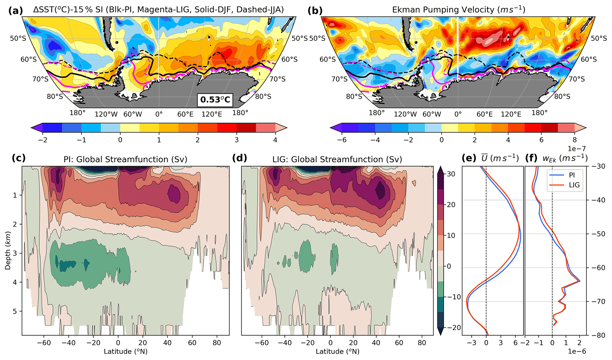
Figure 1Annual mean (a) SST anomalies (∘C) between LIG and PI overlaid with 15 % sea ice concentration (black for PI, magenta for LIG, solid lines for DJF, dashed lines for JJA). The value in the box shows the SO (40–90∘ S) mean ΔSST. (b) Anomalies of the Ekman pumping velocities between LIG and PI (ms−1) overlaid with sea ice concentration (as in a). (c) Global mean meridional streamfunction (Sv) for PI and (d) LIG. Positive values indicate clockwise water mass transport, and negative values indicate anticlockwise transport. Zonal mean (e) winds (ms−1), and (f) Ekman pumping velocities (ms−1) over the SO for PI (blue) and LIG (red).
A 1.5∘ equatorward shift of the SH westerlies is simulated at the LIG (Fig. 1e), with a 10 % weakening of the winds south of 50∘ S. This leads to ∼ 10 % weaker upwelling south of 55∘ S and up to ∼ 20 % stronger upwelling north of 55∘ S (Fig. 1f). Seasonally, the largest changes in upwelling are found for the winter and spring seasons (Fig. A1c and d). The equatorward shift of the westerlies reduces the northward Ekman transport south of 55∘ S, leading to warming, while the higher Ekman transport north of 55∘ S induces a cooling around 50∘ S (Fig. 1a and b). The Antarctic Circumpolar Current is weaker, and the transport through Drake Passage is reduced from PI by ∼ 55 Sv (not shown).
3.2 Response of the air–sea gas exchange
These physical changes in the SO impact the carbon cycle and the air–sea CO2 exchange (Fig. 2). It is worth reiterating here that we analyse changes in the carbon cycle using tracers for a constant atmospheric CO2 concentration of 280 ppm for both simulations (Sect. 2.1), which enables us to solely analyse the impact of climatic and oceanic circulation changes on the carbon cycle. The CO2 flux over the SO at PI shows a carbon uptake near the Antarctic coast, an outgassing band between 65–45∘ S, and another uptake zone further north (Fig. 2a and blue line in d). This CO2 outgassing is due to the upwelling of DIC-rich deep waters (Fig. 1f). At the LIG, the upwelling region widens over the sectors of the Atlantic and Indian oceans, and narrows over the eastern Pacific Ocean sector (Fig. 2). There is a strong increase in outgassing in the sectors of the Atlantic and western Indian oceans, as well as at ∼ 67∘ S in the eastern Pacific Ocean sectors (Fig. 2c and red line in d). An increase in CO2 uptake is simulated in the Amundsen, Bellinghausen, Weddell, Lazarev, Riiser-Larsen, and Ross seas and the subantarctic eastern Pacific (Fig. 2c). The zonal mean CO2 flux in Fig. 2d shows a small increase in uptake south of 62∘ S, possibly due to reduced mixing and reduced winter sea ice cover. Overall, there is a net increase in the mean SO outgassing by ∼ 150 % at the LIG compared to PI (Fig. 2e). This increase in outgassing mostly occurs during the austral winter and spring seasons (Fig. A1e and f).
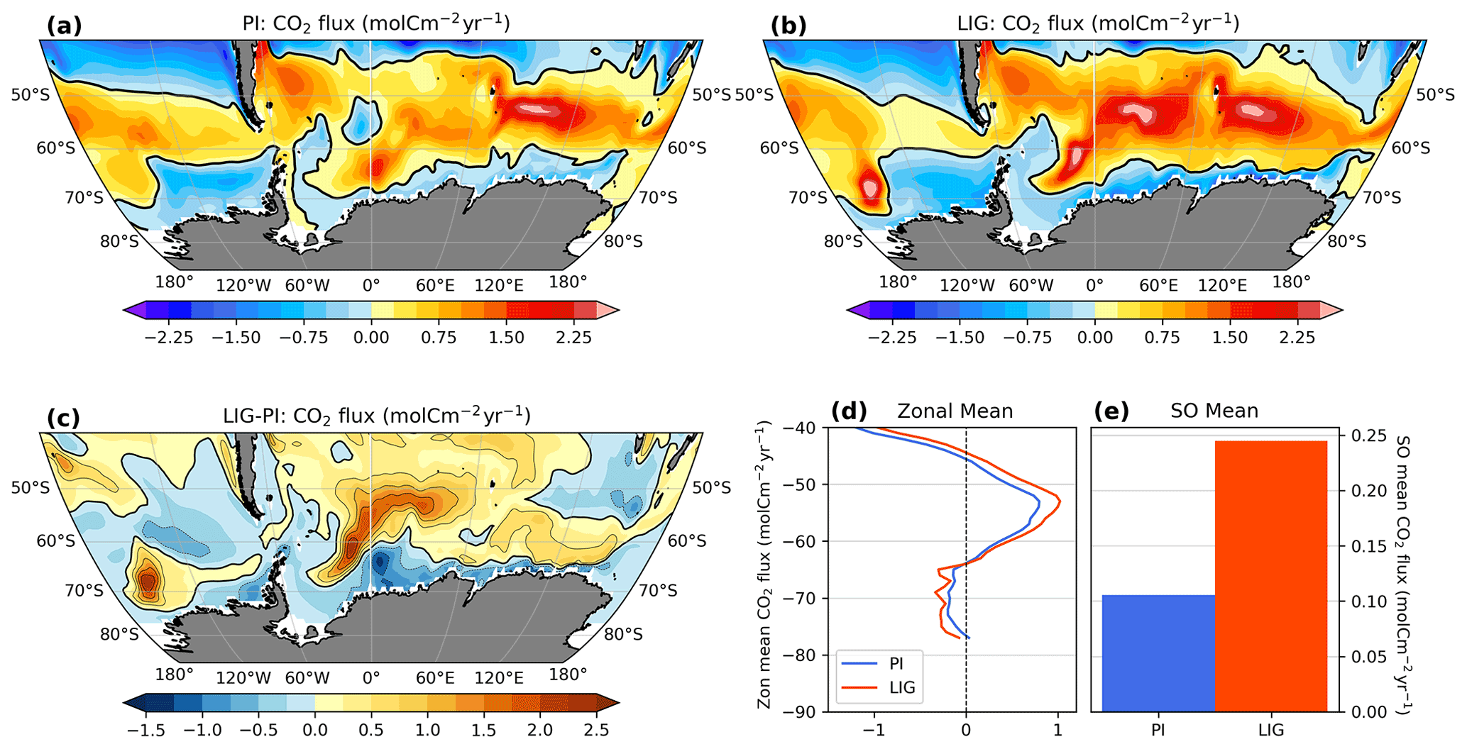
Figure 2Annual mean air–sea CO2 flux (mol C m−2 yr−1) for (a) PI, (b) LIG, and (c) LIG−PI. Red colours indicate outgassing of CO2 from the ocean, and blue colours indicate uptake by the ocean. Thick black lines show the zero line contour. (d) Zonal mean CO2 flux (mol C m−2 yr−1) over the SO for PI (blue) and LIG (red). (e) Mean CO2 flux over the SO (mol C m−2 yr−1) for PI (blue) and LIG (red).
This increased outgassing over the SO is compensated by increased uptake over other ocean basins, especially the North Pacific subpolar gyre, the South Atlantic Ocean, and the Northwest Indian Ocean, while higher outgassing is simulated in the North Atlantic (Fig. A2). In this paper, we focus primarily on the SO. To better understand the SO changes, we decompose the oceanic pCO2 changes into their different components.
3.3 Changes in surface carbon dioxide partial pressure
The air–sea gas exchange is primarily controlled by the seawater partial pressure of CO2 (pCO2). Using the equations presented in Sect. 2.2, Fig. 3 shows a decomposition of the changes in pCO2 into their SST, SSS, DIC, and ALK contributions. In line with the net increase in SO outgassing at the LIG (Fig. 2), the net pCO2 over the SO is 1.2 µatm higher at the LIG compared to PI (black circle) (Fig. 3a). In agreement with the changes in air–sea CO2 flux, surface pCO2 is higher in a zonal band centred at ∼ 55∘ S, while it is lower in coastal regions (contours in Fig. 3b and black line in Fig. 3g). The contributions from individual components add up to reflect the simulated differences reasonably well in terms of both magnitude (1.4 µatm, grey square in Fig. 3a) and spatial distribution (Fig. 3b), affirming the validity of the decomposition method. The overall slightly positive pCO2 anomaly at the LIG compared to PI results from the competing effects of lower CO2 solubility (red triangle, +5.65 µatm) and changes in surface DIC and ALK (blue diamond, −4.25 µatm).
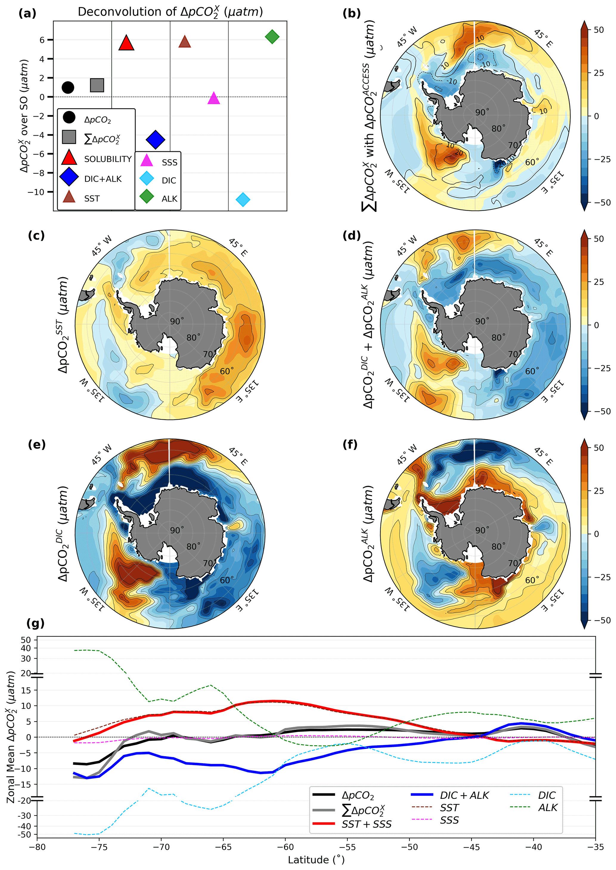
Figure 3Attribution of changes in annual mean surface pCO2 over the SO (µatm). (a) Summary of decomposition of pCO2 over the SO. Simulated difference in pCO2 (black circle) and sum of contributions from all components (grey square, Sect. 2.2). pCO2 change from solubility (SST + SSS, red triangle) and the sum of DIC and ALK components (blue diamond) are given in the same panel. Individual contributions from SST (brown triangle), SSS (magenta triangle), DIC (cyan diamond), and ALK (green diamond) are also shown. (b) Map of the sum of pCO2 contributions from all components (corresponding to grey square in a) in shading, overlaid with the pCO2 change simulated by the model as contours (corresponding to black circle in a). Maps of individual pCO2 contributions from (c) SST (corresponding to the brown triangle in a), (d) DIC and ALK (corresponding to the blue diamond in a), (e) DIC (corresponding to the cyan diamond in a), and (f) ALK (corresponding to the green diamond in a). (g) Zonal mean contributions to pCO2 over the SO (µatm) for simulated ΔpCO2 (black), sum of contributions from all components (grey), solubility (red), sum of DIC and ALK components (blue), SST (dashed brown), SSS (dashed magenta), DIC (dashed cyan), and ALK changes (dashed green) are each shown individually. Note the non-linear scale given for the top and bottom thirds of (g).
The largest contributor to solubility is SST (brown triangle), while the largest contributor of the combined DIC and ALK effect is DIC (cyan diamond in Fig. 3a). Higher SSTs in the SO at the LIG lead to a 5.8 µatm pCO2 increase (brown triangle in Fig. 3a). This SST-induced increase is present over most of the SO and is highest over the South Atlantic, Indian, and West Pacific regions (Fig. 3c). Changes in SSS do not contribute significantly to the pCO2 anomalies (magenta triangle in Figs. 3a and A3d). Changes in DIC cause the largest single contribution to the overall pCO2 change, with the net decrease in surface DIC leading to a −10.9 µatm pCO2 change (cyan diamond in Fig. 3a). As an exception to this, the higher DIC concentrations in the Atlantic Ocean around 55∘ S and in the eastern Pacific sector between 60–70∘ S (Figs. A1g, h, and A4d) lead to higher pCO2 (Fig. 3e). This higher DIC is due to increased upwelling in these regions (Figs. 1b and A1c, d), resulting from the equatorward shift of the SH westerlies. The contributions based on changes in ALK and DIC have very similar patterns, albeit of opposite signs, with a small difference over the West Pacific around 50∘ S. The combined effect of ALK and DIC changes leads to a total net decrease in pCO2 by 4.25 µatm due to the higher impact of changes in DIC (−10.9 µatm, cyan diamond) compared to ALK (+6.65 µatm, green diamond). Overall, south of 45∘ S, changes in SST lead to an overall increase in pCO2, with the highest contributions over the Indian and West Pacific sectors of the SO, while changes in DIC lead to an overall decrease of pCO2, with the strongest reductions in the South Atlantic, Indian, and West Pacific sectors of the SO but an increase in the Amundsen Sea sector (Fig. 3).
The zonal mean patterns of these contributions are presented in Fig. 3g. Coastal regions around Antarctica south of ∼ 75∘ S show that the lower ΔpCO2, both simulated (black line) and calculated (grey line), primarily arise from the combined DIC and ALK component (blue line) that is mainly attributed to the lower DIC (dashed cyan line) compensated by changes in ALK (dashed green line). Between 70 and 60∘ S, ΔpCO2 anomalies are close to zero as the reduced CO2 solubility due to higher SSTs (red line) is compensated by the combined DIC and ALK changes (blue line). Between 60 and 45∘ S, the simulated surface ocean ΔpCO2 is positive (∼ 2 µatm, black line) as the effect of higher SSTs dominates over the combined ALK and DIC components. North of ∼ 45∘ S, the positive ΔpCO2 signal arises from the DIC + ALK component, while solubility mitigates the anomaly (Fig. 3g).
Figure 3g shows that while solubility is mostly controlled by changes in SST, contributions from SSS changes are important south of 72∘ S. Similarly, DIC has the dominant control over the DIC + ALK component. The contributions from both the solubility and (DIC + ALK) components reach their maxima (solubility being positive and DIC + ALK being negative) around 62∘ S, which corresponds to the maximum divergence in wind-driven surface currents (Fig. 1f). To summarize, the higher overall pCO2 (and hence lower air–sea CO2 flux) at the LIG compared to PI can be attributed to higher SSTs south of 45∘ S, and the combined DIC + ALK component between 45 and 35∘ S due to the equatorward shift of the upwelling regions (Fig. 3g). The SST patterns have already been discussed in Sect. 3.1. DIC patterns (Fig. A4d) can result from changes in circulation and the biological pump. These are investigated in the next section.
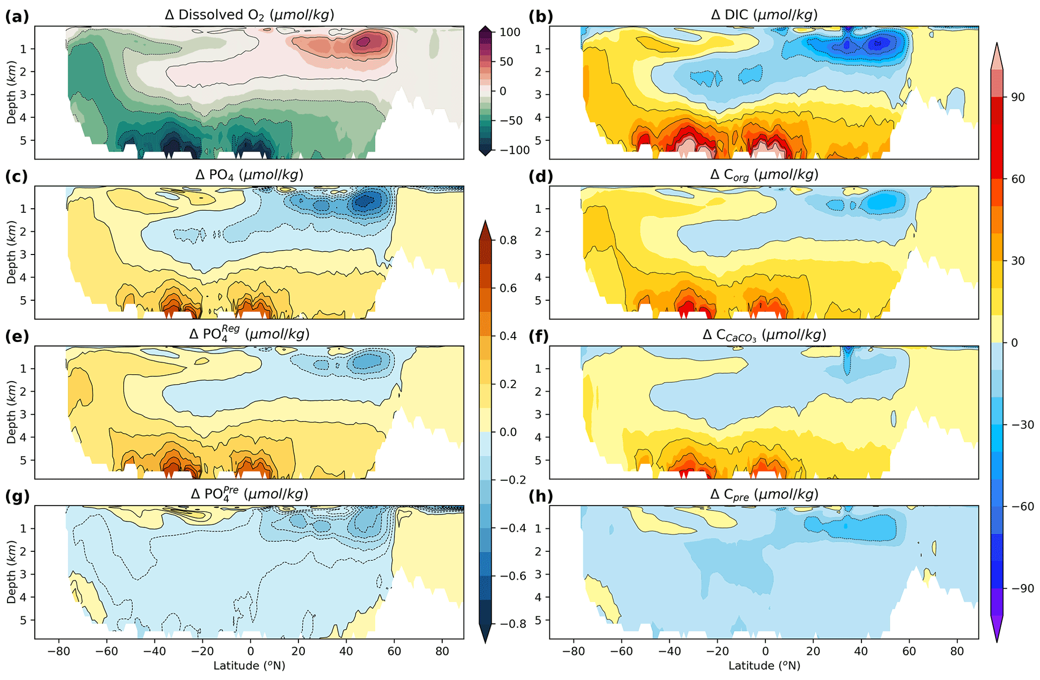
Figure 4Global marine carbon budget and decomposition. Global zonal and annual mean anomalies of (a) dissolved oxygen concentration (µmol kg−1), (c) phosphate concentration (µmol kg−1), (e) regenerated phosphate concentration (µmol kg−1), (g) preformed phosphate concentration (µmol kg−1), (b) total DIC (µmol kg−1), (d) remineralized carbon (µmol kg−1), (f) dissolved carbonate (µmol kg−1), and (h) preformed DIC (µmol kg−1) are given in the individual panels. Note that the phosphate components (c, e, g) and the DIC components (b, d, f, h) each share common colour bars.
3.4 Deep-ocean changes and carbon inventory
Figure 1c and d show that North Atlantic Deep Water (NADW) formation is ∼5 Sv higher in our LIG simulation compared to the PI simulation, leading to colder waters at depths of 1–2 km between 0–60∘ N, accompanied by higher SSTs and SSSs in the Labrador Sea (not shown). We also simulate a ∼ 4 Sv reduction in AABW formation (Fig. 1c and d). This reduction in AABW formation results in a warming of SO deep waters by up to 2 ∘C compared to PI. Due to a northward shift and weakening of winds (Fig. 1e, f), the Antarctic Intermediate Water (AAIW) formation regions shift northward and the AAIW formation rate slows down (Downes et al., 2017). The higher SST, equatorward-shifted upwelling, and reduced sea ice extent lead to an increase in net primary production (NPP) and export production over the SO of ∼ 17 % and ∼ 11 % respectively (Fig. A4a and b).
These circulation changes impact the DIC distribution in the ocean (Fig. 4b). For instance, the reduced formation rate of AAIW (Fig. 1d) increases residence times and leads to lower dissolved oxygen (Fig. 4a), higher PO4 (Fig. 4c), higher remineralized carbon (Fig. 4d), and higher DIC concentrations (Fig. 4b) at intermediate depths of the SO north of 55∘ S. Similarly, the increased accumulation of nutrients and DIC, as well as oxygen depletion in deep and abyssal waters (Fig. 4a, b and c), can be attributed to a weaker AABW formation rate (Fig. 1d), which results in a higher efficiency of the biological pump, as detailed below.
The ACCESS-ESM1.5 simulates a ≥50 µmol kg−1 decrease in oxygen everywhere below 3 km at the LIG compared to PI. A decrease in oxygen can also be seen in the SO across all depths, including a northward-reaching tongue attributable to AAIW at ∼ 1 km depth extending to the Equator (Fig. 4a). DIC anomalies follow the patterns of dissolved oxygen, albeit with the opposite sign. The simulated DIC concentrations are ∼ 50 µmol kg−1 higher across all depths in the SO and globally below 3.5 km depth (Fig. 4b).
DIC anomalies are decomposed into contributions from remineralized organic carbon, dissolved calcium carbonate, and preformed carbon components (Fig. 4d, f and h, Sect. 2.3). A total of 60 % of the DIC increase in the SO and abyssal ocean can be attributed to an increase in remineralized carbon (Fig. 4d) resulting from a 10 % more efficient biological pump (Eq. 6, Sect. 2.3). This increase in remineralized carbon can be attributed to increased residence times, which are in turn due to weaker bottom- and intermediate-water formation rates (Fig. 1c and d). Weaker AABW and AAIW indeed lead to positive apparent oxygen utilization (AOU) and regenerated PO4 anomalies (Fig. 4e). In addition, a 2 ∘C warming of bottom waters leads to a ∼ 6 % increase in remineralization rates, thus further contributing to the higher remineralized carbon. Around 25 % of the abyssal increase in DIC is attributed to the carbonate pump (Fig. 4f). This reflects changes in NPP, export production (Fig. A4), and water mass residence times, given that carbonate production is a constant percentage of total NPP in this model setup and carbonate dissolution is constant and independent of water chemistry or temperature. Preformed DIC represents only ∼ 5 % of the DIC changes (Fig. 4h). This increased sequestration of DIC in the deep ocean reduces the surface DIC concentration (Figs. A4 and A1g, h), thus contributing to a lowering of surface pCO2 (Fig. 3e and g).
For the Northern Hemisphere, stronger NADW (Fig. 1c and d) results in decreased DIC concentrations in intermediate and deep waters of the North Atlantic by up to 75 µmol kg−1 (Fig. 4b). This negative DIC anomaly can be explained by a decrease in both remineralized and preformed DIC. Stronger NADW subducts more DIC-depleted surface waters into the deep ocean (Duteil et al., 2012) and reduces residence times, thus leading to a decrease in remineralized carbon. This is also associated with a ∼ 40 µmol kg−1 increase in dissolved oxygen content (Fig. 4a) and an up to 0.75 µmol kg−1 decrease in PO4 concentration (Fig. 4c). The reduction in preformed carbon (Fig. 4h) is most likely due to a new NADW formation site in the Labrador Sea and a slight northward shift of the deep-water formation regions in the Norwegian and Greenland seas.
We analyse the SO marine carbon cycle response to warmer conditions as simulated in an equilibrium simulation of the LIG. The lig127k simulation performed with the ACCESS-ESM1.5 presented here displays an annual mean warming of 0.53 ∘C at the surface of the SO compared to PI. This simulated southern high-latitude warming (Fig. 1a) is in agreement with the multi-model mean of the PMIP4 lig127k simulations, although it is at the higher end of the spectrum (Otto-Bliesner et al., 2021). Seasonally, we simulate regional SSTs up to 4 ∘C higher around 60∘ S for both the austral spring and summer, in line with both proxy records (Capron et al., 2017; Hoffman et al., 2017) and the PMIP3 125 ka experiment performed with the NORESM-1ME model (Kessler et al., 2018), while the PMIP4 lig127k multi-model mean for austral summer displays less than 0.5 ∘C warming over the SO (Otto-Bliesner et al., 2021). The simulated SO sea ice concentration at the LIG for austral winter (Figs. 1 and A1) is also in good agreement with those inferred in previous studies (Holloway et al., 2016, 2017), even though the changes in Antarctic sea ice area of the ACCESS-ESM1.5 are the largest amongst all the CMIP6-PMIP4 models (Otto-Bliesner et al., 2021).
A 1.5∘ equatorward shift of the westerlies, resulting in a 10 % weakening of the westerlies south of 50∘ S, is simulated at the LIG (Fig. 1e), leading to significant changes in SO upwelling (Fig. 1b and f). There is no clear consensus for position and strength of the SH westerlies during the LIG (Fogwill et al., 2014), although the higher obliquity might have led to a weakening of the westerlies compared to PI (Timmermann et al., 2014). These changes in winds lead to a northward shift of the AAIW formation regions. Our LIG simulation is also characterized by a weakening of AABW formation rates, which might be due to changes in surface density. Significant weakening of AABW during the LIG due to Antarctic meltwater discharge has previously been inferred from paleo-proxy records (Hayes et al., 2014; Rohling et al., 2019). A shift in westerlies might also contribute to a weakening of the AABW (Menviel et al., 2008; Huiskamp et al., 2016; Glasscock et al., 2020).
The reduced upwelling south of 55∘ S and weaker AABW transport simulated here lead to an increased sequestration of DIC in the deep ocean, through an increase in the efficiency of the biological pump (Fig. 4). This reduces the surface DIC concentrations, leading to a net reduction in outgassing over the SO, as has been previously hypothesized (Toggweiler et al., 2006). However, while the combined DIC and ALK contributions would lead to a lower pCO2 at the surface of the SO, this change is overcompensated by the warmer conditions (Fig. 3). Reduced solubility due to higher SSTs leads to an increase in outgassing over most of the SO, while the reduced sea ice cover does not seem to significantly impact the CO2 fluxes. Assessing the impact of sea ice changes on CO2 fluxes (Appendix A), we find that reduced sea ice concentration at the LIG in the Weddell and Ross seas leads to a 5 % increase in CO2 uptake in autumn and winter (Fig. A5). Reduced solubility results in a net outgassing of CO2 over the SO, with a ∼150% increase at the LIG compared to PI (Fig. 2), and the largest increase over the austral winter and spring seasons (Fig. A1). The simulated NPP and export production are ∼17% and ∼ 11 % higher, respectively, over the SO at the LIG compared to PI (Fig. A4), providing a negative feedback to the higher outgassing. Although the simulated nutrient and alkalinity concentrations are underestimated over the SO, the vertical gradients of these are captured reasonably well (Ziehn et al., 2020). As such, these biases should not significantly impact our results. All of our analysis is based on a constant atmospheric CO2 concentration of 280 ppm to allow quantification of the effects of the LIG climate on the carbon cycle independently of the background CO2 concentration. However, this constant atmospheric CO2 concentration neglects feedbacks related to CO2 uptake and outgassing. Nevertheless, the lower CO2 at LIG (275 ppm) compared to PI (284.3 ppm) would suggest the LIG SO to be an even greater CO2 source to the atmosphere, implying a stronger sink somewhere else in the ocean or on land (Brovkin et al., 2016).
Numerical studies have unequivocally shown the impact of changes in the magnitude of the westerlies on the carbon cycle, with stronger westerlies leading to increased upwelling and SO outgassing and vice-versa (e.g. Menviel et al., 2008, 2018; d'Orgeville et al., 2010; Lauderdale et al., 2013, 2017; Huiskamp et al., 2016; Gottschalk et al., 2019); however, the impact of changes in the latitudinal position of the westerlies on the carbon cycle is less certain (e.g. d'Orgeville et al., 2010; Völker and Köhler, 2013; Lauderdale et al., 2013; Huiskamp et al., 2016; Gottschalk et al., 2019). Given the simulated increase in DIC content in the deeper SO and the reduced DIC at the surface of the SO, our simulations suggest that the simulated equatorward shift of the westerlies reduces the SO CO2 outgassing.
SH westerlies are projected to strengthen and shift poleward over the coming century (Collins et al., 2013; Zheng et al., 2013; Goyal et al., 2021), contrary to the LIG simulations presented here. An increase in SO NPP at the LIG is simulated here, in line with CMIP6 projections of the coming century (Kwiatkowski et al., 2020). Thus, changes in the carbon cycle simulated at the LIG may not serve as a good analogue for potential future changes. Nevertheless, the simulated enhanced SO CO2 outgassing, despite a slight equatorward shift of the westerlies, supports a weaker capability of the Southern Ocean to take up anthropogenic CO2 over the coming century.
To estimate the effect of sea ice changes at the LIG on the air–sea gas exchange, we use a modified version of the equation of CO2 flux from Wanninkhof (2014):
where is the CO2 flux (mol C m−2 yr−1), U is the average wind speed (m s−1), ΔpCO2 is the difference in partial pressure of CO2 between ocean surface and atmosphere (µatm), and Sc is the sea ice concentration. To investigate the effect of LIG sea ice changes on the LIG CO2 flux, we estimate using both LIG Sc and PI Sc, while keeping all the other variables at LIG values. The resulting patterns are presented in Fig. A5. Figure A5 shows that the reduced sea ice during LIG compared to PI leads to a less than 5 % increase in carbon sink over the Ross Sea region all year round and over the Weddell Sea region in autumn and winter and an around 2 % increase in outgassing in the Lazarev and Weddell seas.

Figure A1Seasonal anomalies for austral winter, (JJA, a, c, e, g) and austral spring (SON, b, d, f, h) of (a, b) SST (∘C) overlaid with 50 % sea ice concentration (dashed for PI and solid for LIG), (c, d) Ekman pumping velocities (ms−1) overlaid with 50 % sea ice concentration (dashed for PI and solid for LIG), (e, f) sea–air CO2 flux (mol C m−2 yr−1, with positive indicating outgassing from and negative indicating uptake by the ocean), and (g, h) surface DIC concentrations (µmol kg−1).
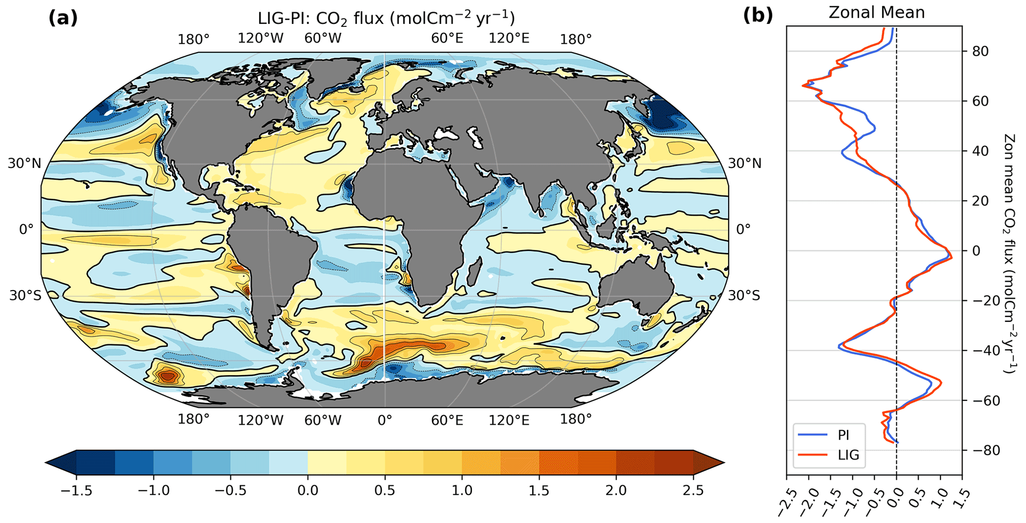
Figure A2(a) Annual mean air–sea CO2 flux (mol C m−2 yr−1) for LIG−PI. Red colours indicate outgassing of CO2 from the ocean, and blue colours indicate uptake by the ocean. Thick black lines show the zero line contour. (b) Zonal mean CO2 flux (mol C m−2 yr−1) for PI (blue) and LIG (red).


Figure A4Changes in annual mean productivity and related variables. (a) Anomalies of depth-integrated annual mean NPP (as chlorophyll in seawater, kg m−3) overlaid with 15 % sea ice concentration (black for PI, red for LIG, solid lines for DJF, and dashed lines for JJA). (b) Anomalies of annual mean detrital concentration at 200 m depth (kg m−3) overlaid with sea ice (same as a). (c) Anomalies of annual mean surface phosphate concentrations (µmol kg−1) overlaid with sea ice (same as a). (d) Anomalies of annual mean surface DIC concentrations (µmol kg−1) overlaid with sea ice (same as a).
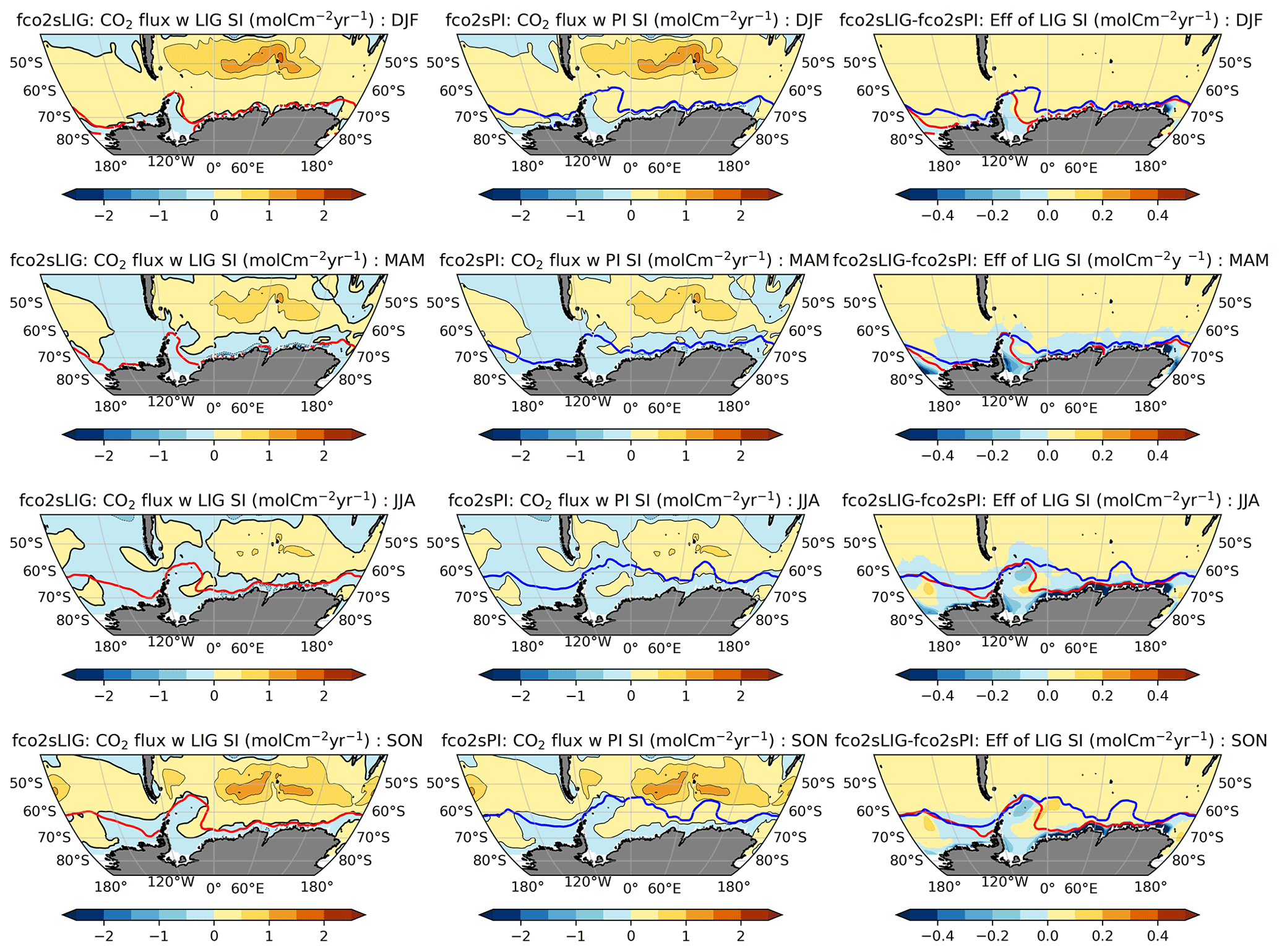
Figure A5Calculated seasonal CO2 fluxes using LIG ΔpCO2, winds and (left) LIG sea-ice concentration, (middle) PI sea ice concentrations, and (right) differences in CO2 flux for calculations using the LIG sea ice concentrations compared to PI sea ice concentrations. Note the reduced colour scale in the right-hand column. Calculations are based on Wanninkhof (1992) and Wanninkhof (2014). The red and blue contours indicate 15 % sea ice concentrations for LIG and PI, respectively.
Outputs of the variables from the lig127k simulation used in this paper are archived on the CMIP6 ESGF website at https://doi.org/10.22033/ESGF/CMIP6.13703 (Yeung et al., 2019).
DC performed all of the analysis and writing of the results. LM and KJM provided support with the interpretation and writing of the results. NKHY performed the lig127k simulation. MC and TZ contributed to the model setup and troubleshooting. All authors contributed towards the final manuscript.
At least one of the co-authors is a member of the editorial board of Climate of the Past. The peer-review process was guided by an independent editor, and the authors also have no other competing interests to declare.
Publisher's note: Copernicus Publications remains neutral with regard to jurisdictional claims in published maps and institutional affiliations.
The simulations were conducted and analysed at the National Computing Infrastructure (NCI) National Facility at the Australian National University, through awards under the Merit Allocation Scheme, the Intersect Allocation Scheme, and the UNSW HPC at NCI scheme.
This research has been supported by the Australian Research Council (grant nos. DP180100048 and FT180100606).
This paper was edited by Qiuzhen Yin and reviewed by two anonymous referees.
Behrenfeld, M. J. and Falkowski, P. G.: Photosynthetic rates derived from satellite-based chlorophyll concentration, Limnol. Oceanogr., 42, 1–20, 1997.
Berger, A.: Long-term variations of daily insolation and Quaternary climatic changes, J. Atmos. Sci., 35, 2362–2367, 1978.
Bernardello, R., Marinov, I., Palter, J. B., Sarmiento, J. L., Galbraith, E. D., and Slater, R. D.: Response of the ocean natural carbon storage to projected twenty-first-century climate change, J. Climate, 27, 2033–2053, 2014.
Boyd, P. W.: Toward quantifying the response of the oceans' biological pump to climate change, Front. Mar. Sci., 2, 77, 2015.
Bracegirdle, T. J., Krinner, G., Tonelli, M., Haumann, F. A., Naughten, K. A., Rackow, T., Roach, L. A., and Wainer, I.: Twenty first century changes in Antarctic and Southern Ocean surface climate in CMIP6, Atmos. Sci. Lett., 21, e984, https://doi.org/10.1002/asl.984, 2020.
Brovkin, V., Brücher, T., Kleinen, T., Zaehle, S., Joos, F., Roth, R., Spahni, R., Schmitt, J., Fischer, H., Leuenberger, M., Stone, E. J., Ridgwell, A., Chappellaz, J., Kehrwald, N., Barbante, C., Blunier, T., and Dahl Jensen, D.: Comparative carbon cycle dynamics of the present and last interglacial, Quaternary Sci. Rev., 137, 15–32, https://doi.org/10.1016/j.quascirev.2016.01.028, 2016.
Caldeira, K. and Duffy, P. B.: The role of the Southern Ocean in uptake and storage of anthropogenic carbon dioxide, Science, 287, 620–622, 2000.
CAPE-Last Interglacial Project Members: Last Interglacial Arctic warmth confirms polar amplification of climate change, Quaternary Sci. Rev., 25, 1383–1400, 2006.
Capron, E., Govin, A., Stone, E. J., Masson-Delmotte, V., Mulitza, S., Otto-Bliesner, B., Rasmussen, T. L., Sime, L. C., Waelbroeck, C., and Wolff, E. W.: Temporal and spatial structure of multi-millennial temperature changes at high latitudes during the Last Interglacial, Quaternary Sci. Rev., 103, 116–133, 2014.
Capron, E., Govin, A., Feng, R., Otto-Bliesner, B. L., and Wolff, E.: Critical evaluation of climate syntheses to benchmark CMIP6/PMIP4 127 ka Last Interglacial simulations in the high-latitude regions, Quaternary Sci. Rev., 168, 137–150, 2017.
Collins, M., Knutti, R., Arblaster, J., Dufresne, J.-L., Fichefet, T., Friedlingstein, P., Gao, X., Gutowski, W. J., Johns, T., Krinner, G., Shongwe, M., Tebaldi, C., Weaver, A. J., Wehner, M. F., Allen, M. R., Andrews, T., Beyerle, U., Bitz, C. M., Bony, S., and Booth, B. B. B.: Long-term climate change: projections, commitments and irreversibility, in: Climate Change 2013 – The Physical Science Basis: Contribution of Working Group I to the Fifth Assessment Report of the Intergovernmental Panel on Climate Change, edited by: Stocker, T. F., Qin, D., Plattner, G.-K., Tignor, M. M. B., Allen, S. K., Boschung, J., Nauels, A., Xia, Y., Bex, V., and Midgley, P. M., 1029–1136, Cambridge University Press, 2013.
Craig, A., Valcke, S., and Coquart, L.: Development and performance of a new version of the OASIS coupler, OASIS3-MCT_3.0, Geosci. Model Dev., 10, 3297–3308, https://doi.org/10.5194/gmd-10-3297-2017, 2017.
Dahl-Jensen, D., Albert, M., Aldahan, A., Azuma, N., Balslev-Clausen, D., Baumgartner, M., Berggren, A.-M., Bigler, M., Binder, T., Blunier, T., and Bourgeois, J. C.: Eemian interglacial reconstructed from a Greenland folded ice core, Nature, 493, 489–494, 2013.
DeVries, T.: The oceanic anthropogenic CO2 sink: Storage, air-sea fluxes, and transports over the industrial era, Global Biogeochem. Cy., 28, 631–647, 2014.
d'Orgeville, M., Sijp, W., England, M., and Meissner, K.: On the control of glacial-interglacial atmospheric CO2 variations by the Southern Hemisphere westerlies, Geophys. Res. Lett., 37, L21703, https://doi.org/10.1029/2010GL045261, 2010.
Downes, S. M., Langlais, C., Brook, J. P., and Spence, P.: Regional impacts of the westerly winds on Southern Ocean mode and intermediate water subduction, J. Phys. Oceanogr., 47, 2521–2530, 2017.
Duteil, O., Koeve, W., Oschlies, A., Aumont, O., Bianchi, D., Bopp, L., Galbraith, E., Matear, R., Moore, J. K., Sarmiento, J. L., and Segschneider, J.: Preformed and regenerated phosphate in ocean general circulation models: can right total concentrations be wrong?, Biogeosciences, 9, 1797–1807, https://doi.org/10.5194/bg-9-1797-2012, 2012.
Dutton, A., Carlson, A. E., Long, A., Milne, G. A., Clark, P. U., DeConto, R., Horton, B. P., Rahmstorf, S., and Raymo, M. E.: Sea-level rise due to polar ice-sheet mass loss during past warm periods, Science, 349, p. aaa4019, 2015.
Dyer, B., Austermann, J., D’Andrea, W. J., Creel, R. C., Sandstrom, M. R., Cashman, M., Rovere, A., and Raymo, M. E.: Sea-level trends across The Bahamas constrain peak last interglacial ice melt, P. Natl. Acad. Sci. USA, 118, e2026839118, https://doi.org/10.1073/pnas.2026839118, 2021.
Egleston, E. S., Sabine, C. L., and Morel, F. M.: Revelle revisited: Buffer factors that quantify the response of ocean chemistry to changes in DIC and alkalinity, Global Biogeochem. Cy., 24, GB1002, https://doi.org/10.1029/2008GB003407, 2010.
Eyring, V., Bony, S., Meehl, G. A., Senior, C. A., Stevens, B., Stouffer, R. J., and Taylor, K. E.: Overview of the Coupled Model Intercomparison Project Phase 6 (CMIP6) experimental design and organization, Geosci. Model Dev., 9, 1937–1958, https://doi.org/10.5194/gmd-9-1937-2016, 2016.
Fan, X., Duan, Q., Shen, C., Wu, Y., and Xing, C.: Global surface air temperatures in CMIP6: historical performance and future changes, Environ. Res. Lett., 15, 104056, https://doi.org/10.1088/1748-9326/abb051, 2020.
Fetterer, F., Knowles, K., Meier, W., Savoie, M., and Windnagel, A.: Updated daily sea ice index, version 3, sea ice concentration, Boulder, Colorado, USA, NSIDC: National Snow and Ice Data Center [data set], https://nsidc.org/data/G02135/versions/3 (last access: 11 November 2019) 2017.
Fogwill, C. J., Turney, C. S., Meissner, K. J., Golledge, N. R., Spence, P., Roberts, J. L., England, M. H., Jones, R. T., and Carter, L.: Testing the sensitivity of the East Antarctic Ice Sheet to Southern Ocean dynamics: past changes and future implications, J. Quaternary Sci., 29, 91–98, 2014.
Friedlingstein, P., O'Sullivan, M., Jones, M. W., Andrew, R. M., Hauck, J., Olsen, A., Peters, G. P., Peters, W., Pongratz, J., Sitch, S., Le Quéré, C., Canadell, J. G., Ciais, P., Jackson, R. B., Alin, S., Aragão, L. E. O. C., Arneth, A., Arora, V., Bates, N. R., Becker, M., Benoit-Cattin, A., Bittig, H. C., Bopp, L., Bultan, S., Chandra, N., Chevallier, F., Chini, L. P., Evans, W., Florentie, L., Forster, P. M., Gasser, T., Gehlen, M., Gilfillan, D., Gkritzalis, T., Gregor, L., Gruber, N., Harris, I., Hartung, K., Haverd, V., Houghton, R. A., Ilyina, T., Jain, A. K., Joetzjer, E., Kadono, K., Kato, E., Kitidis, V., Korsbakken, J. I., Landschützer, P., Lefèvre, N., Lenton, A., Lienert, S., Liu, Z., Lombardozzi, D., Marland, G., Metzl, N., Munro, D. R., Nabel, J. E. M. S., Nakaoka, S.-I., Niwa, Y., O'Brien, K., Ono, T., Palmer, P. I., Pierrot, D., Poulter, B., Resplandy, L., Robertson, E., Rödenbeck, C., Schwinger, J., Séférian, R., Skjelvan, I., Smith, A. J. P., Sutton, A. J., Tanhua, T., Tans, P. P., Tian, H., Tilbrook, B., van der Werf, G., Vuichard, N., Walker, A. P., Wanninkhof, R., Watson, A. J., Willis, D., Wiltshire, A. J., Yuan, W., Yue, X., and Zaehle, S.: Global Carbon Budget 2020, Earth Syst. Sci. Data, 12, 3269–3340, https://doi.org/10.5194/essd-12-3269-2020, 2020.
Galaasen, E. V., Ninnemann, U. S., Irvalı, N., Kleiven, H. K. F., Rosenthal, Y., Kissel, C., and Hodell, D. A.: Rapid reductions in North Atlantic Deep Water during the peak of the last interglacial period, Science, 343, 1129–1132, 2014.
Garcia, H., Locarnini, R., and Boyer, T.: World Ocean Atlas 2009, Volume 3: Dissolved Oxygen, Apparent Oxygen Utilization, and Oxygen Saturation, S. Levitus, Ed. NOAA Atlas NESDIS 70, US, 2010a.
Garcia, H., Locarnini, R., Boyer, T., Antonov, J., Zweng, M., Baranova, O., and Johnson, D.: World Ocean Atlas 2009, volume 4: Nutrients (phosphate, nitrate, silicate), NOAA Atlas NESDIS 71, S. Levitus), Washington, DC: US Government Printing Office, 2010b.
Glasscock, S., Hayes, C., Redmond, N., and Rohde, E.: Changes in Antarctic Bottom Water formation during interglacial periods, Paleoceanogr. Paleoclimatol., 35, e2020PA003867, https://doi.org/10.1029/2020PA003867, 2020.
Gottschalk, J., Battaglia, G., Fischer, H., Frölicher, T. L., Jaccard, S. L., Jeltsch-Thömmes, A., Joos, F., Köhler, P., Meissner, K. J., Menviel, L., Nehrbass-Ahles, C., Schmitt, J., Schmittner, A., Skinner, L. C., and Stocker, T. F.: Mechanisms of millennial-scale atmospheric CO2 change in numerical model simulations, Quaternary Sci. Rev., 220, 30–74, https://doi.org/10.1016/j.quascirev.2019.05.013, 2019.
Govin, A., Braconnot, P., Capron, E., Cortijo, E., Duplessy, J.-C., Jansen, E., Labeyrie, L., Landais, A., Marti, O., Michel, E., Mosquet, E., Risebrobakken, B., Swingedouw, D., and Waelbroeck, C.: Persistent influence of ice sheet melting on high northern latitude climate during the early Last Interglacial, Clim. Past, 8, 483–507, https://doi.org/10.5194/cp-8-483-2012, 2012.
Goyal, R., Sen Gupta, A., Jucker, M., and England, M. H.: Historical and projected changes in the Southern Hemisphere surface westerlies, Geophys. Res. Lett., 48, e2020GL090849, https://doi.org/10.1029/2020GL090849, 2021.
Griffies, S.: Elements of the Modular Ocean Model (MOM) 5: (2012 release with updates). GFDL Ocean Group Tech. Rep. 7, NOAA, Geophysical Fluid Dynamics Laboratory, Princeton, NJ, 618, 2014.
Gruber, N., Clement, D., Carter, B. R., Feely, R. A., Van Heuven, S., Hoppema, M., Ishii, M., Key, R. M., Kozyr, A., Lauvset, S. K., and Lo Monaco, C.: The oceanic sink for anthropogenic CO2 from 1994 to 2007, Science, 363, 1193–1199, 2019a.
Gruber, N., Landschützer, P., and Lovenduski, N. S.: The variable Southern Ocean carbon sink, Annu. Rev. Mar. Sci., 11, 159–186, 2019b.
Hayes, C. T., Martínez-García, A., Hasenfratz, A. P., Jaccard, S. L., Hodell, D. A., Sigman, D. M., Haug, G. H., and Anderson, R. F.: A stagnation event in the deep South Atlantic during the last interglacial period, Science, 346, 1514–1517, 2014.
Hoffman, J. S., Clark, P. U., Parnell, A. C., and He, F.: Regional and global sea-surface temperatures during the last interglaciation, Science, 355, 276–279, 2017.
Holland, M. M. and Bitz, C. M.: Polar amplification of climate change in coupled models, Clim. Dynam., 21, 221–232, 2003.
Holloway, M. D., Sime, L. C., Singarayer, J. S., Tindall, J. C., Bunch, P., and Valdes, P. J.: Antarctic last interglacial isotope peak in response to sea ice retreat not ice-sheet collapse, Nat. Commun., 7, 1–9, 2016.
Holloway, M. D., Sime, L. C., Allen, C. S., Hillenbrand, C.-D., Bunch, P., Wolff, E., and Valdes, P. J.: The spatial structure of the 128 ka Antarctic sea ice minimum, Geophys. Res. Lett., 44, 11–129, 2017.
Howes, E. L., Joos, F., Eakin, M., and Gattuso, J.-P.: An updated synthesis of the observed and projected impacts of climate change on the chemical, physical and biological processes in the oceans, Front. Mar. Sci., 2, 1–7, https://doi.org/10.3389/fmars.2015.00036, 2015.
Huiskamp, W., Meissner, K., and d’Orgeville, M.: Competition between ocean carbon pumps in simulations with varying Southern Hemisphere westerly wind forcing, Clim. Dynam., 46, 3463–3480, 2016.
Hunke, E. C., Lipscomb, W. H., Turner, A. K., Jeffery, N., and Elliott, S.: CICE: the Los Alamos sea ice model documentation and software user’s manual version 4.1 la-cc-06-012, T-3 Fluid Dynamics Group, Los Alamos National Laboratory, 675, 500, 2010.
Ito, T. and Follows, M. J.: Preformed phosphate, soft tissue pump and atmospheric CO2, J. Mar. Res., 63, 813–839, 2005.
Jiang, L.-Q., Carter, B. R., Feely, R. A., Lauvset, S. K., and Olsen, A.: Surface ocean pH and buffer capacity: past, present and future, Sci. Rep., 9, 1–11, 2019.
Kageyama, M., Sime, L. C., Sicard, M., Guarino, M.-V., de Vernal, A., Stein, R., Schroeder, D., Malmierca-Vallet, I., Abe-Ouchi, A., Bitz, C., Braconnot, P., Brady, E. C., Cao, J., Chamberlain, M. A., Feltham, D., Guo, C., LeGrande, A. N., Lohmann, G., Meissner, K. J., Menviel, L., Morozova, P., Nisancioglu, K. H., Otto-Bliesner, B. L., O'ishi, R., Ramos Buarque, S., Salas y Melia, D., Sherriff-Tadano, S., Stroeve, J., Shi, X., Sun, B., Tomas, R. A., Volodin, E., Yeung, N. K. H., Zhang, Q., Zhang, Z., Zheng, W., and Ziehn, T.: A multi-model CMIP6-PMIP4 study of Arctic sea ice at 127 ka: sea ice data compilation and model differences, Clim. Past, 17, 37–62, https://doi.org/10.5194/cp-17-37-2021, 2021.
Kessler, A., Galaasen, E. V., Ninnemann, U. S., and Tjiputra, J.: Ocean carbon inventory under warmer climate conditions – the case of the Last Interglacial, Clim. Past, 14, 1961–1976, https://doi.org/10.5194/cp-14-1961-2018, 2018.
Key, R. M., Kozyr, A., Sabine, C. L., Lee, K., Wanninkhof, R., Bullister, J. L., Feely, R. A., Millero, F. J., Mordy, C., and Peng, T.-H.: A global ocean carbon climatology: Results from Global Data Analysis Project (GLODAP), Global Biogeochem. Cy., 18, 0886–6236, https://doi.org/10.1029/2004GB002247, 2004.
Kleinen, T., Brovkin, V., and Munhoven, G.: Modelled interglacial carbon cycle dynamics during the Holocene, the Eemian and Marine Isotope Stage (MIS) 11, Clim. Past, 12, 2145–2160, https://doi.org/10.5194/cp-12-2145-2016, 2016.
Kowalczyk, E., Stevens, L., Law, R., Dix, M., Wang, Y., Harman, I., Haynes, K., Srbinovsky, J., Pak, B., and Ziehn, T.: The land surface model component of ACCESS: description and impact on the simulated surface climatology, Aust. Meteorol. Oceanogr. J, 63, 65–82, 2013.
Kwiatkowski, L., Torres, O., Bopp, L., Aumont, O., Chamberlain, M., Christian, J. R., Dunne, J. P., Gehlen, M., Ilyina, T., John, J. G., Lenton, A., Li, H., Lovenduski, N. S., Orr, J. C., Palmieri, J., Santana-Falcón, Y., Schwinger, J., Séférian, R., Stock, C. A., Tagliabue, A., Takano, Y., Tjiputra, J., Toyama, K., Tsujino, H., Watanabe, M., Yamamoto, A., Yool, A., and Ziehn, T.: Twenty-first century ocean warming, acidification, deoxygenation, and upper-ocean nutrient and primary production decline from CMIP6 model projections, Biogeosciences, 17, 3439–3470, https://doi.org/10.5194/bg-17-3439-2020, 2020.
Landschuetzer, P., Gruber, N., and Bakker, D. C.: Decadal variations and trends of the global ocean carbon sink, Global Biogeochem. Cy., 30, 1396–1417, 2016.
Laskar, J., Robutel, P., Joutel, F., Gastineau, M., Correia, A., and Levrard, B.: A long-term numerical solution for the insolation quantities of the Earth, Astro. Astrophys., 428, 261–285, 2004.
Lauderdale, J. M., Garabato, A. C. N., Oliver, K. I., Follows, M. J., and Williams, R. G.: Wind-driven changes in Southern Ocean residual circulation, ocean carbon reservoirs and atmospheric CO2, Clim. Dynam., 41, 2145–2164, 2013.
Lauderdale, J. M., Williams, R. G., Munday, D. R., and Marshall, D. P.: The impact of Southern Ocean residual upwelling on atmospheric CO2 on centennial and millennial timescales, Clim. Dynam., 48, 1611–1631, 2017.
Law, R. M., Ziehn, T., Matear, R. J., Lenton, A., Chamberlain, M. A., Stevens, L. E., Wang, Y.-P., Srbinovsky, J., Bi, D., Yan, H., and Vohralik, P. F.: The carbon cycle in the Australian Community Climate and Earth System Simulator (ACCESS-ESM1) – Part 1: Model description and pre-industrial simulation, Geosci. Model Dev., 10, 2567–2590, https://doi.org/10.5194/gmd-10-2567-2017, 2017.
Le Quéré, C., Rödenbeck, C., Buitenhuis, E. T., Conway, T. J., Langenfelds, R., Gomez, A., Labuschagne, C., Ramonet, M., Nakazawa, T., Metzl, N., and Gillett, N.: Saturation of the Southern Ocean CO2 sink due to recent climate change, Science, 316, 1735–1738, https://doi.org/10.1126/science.1136188, 2007.
Lovenduski, N. S., Gruber, N., Doney, S. C., and Lima, I. D.: Enhanced CO2 outgassing in the Southern Ocean from a positive phase of the Southern Annular Mode, Global Biogeochem. Cy., 21, 0886–6236, https://doi.org/10.1029/2006GB002900, 2007.
Martin, G., Milton, S., Senior, C., Brooks, M., Ineson, S., Reichler, T., and Kim, J.: Analysis and reduction of systematic errors through a seamless approach to modeling weather and climate, J. Climate, 23, 5933–5957, 2010.
Masson-Delmotte, V., Schulz, M., Abe-Ouchi, A., Beer, J., Ganopolski, A., Rouco, J. G., Jansen, E., Lambeck, K., Luterbacher, J., Naish, T., and Osborn, T.: Information from Paleoclimate Archives, in: Climate Change 2013: The Physical Science Basis Contribution of Working Group I to the Fifth Assessment Report of the Intergovernmental Panel on Climate Change, edited by: Stocker, T. F., Qin, D., Plattner, G.-K., Tignor, M., Allen, S. K., Boschung, J., Nauels, A., Xia, Y., Bex, V. and Midgley, P. M., Cambridge, United Kingdom and New York, NY, USA, 435, 2013.
Menviel, L., Timmermann, A., Mouchet, A., and Timm, O.: Climate and marine carbon cycle response to changes in the strength of the Southern Hemispheric westerlies, Paleoceanography, 23, 0883–8305, https://doi.org/10.1029/2008PA001604, 2008.
Menviel, L., Spence, P., Yu, J., Chamberlain, M., Matear, R., Meissner, K., and England, M. H.: Southern Hemisphere westerlies as a driver of the early deglacial atmospheric CO2 rise, Nat. Commun., 9, 1–12, 2018.
Oke, P. R., Griffin, D. A., Schiller, A., Matear, R. J., Fiedler, R., Mansbridge, J., Lenton, A., Cahill, M., Chamberlain, M. A., and Ridgway, K.: Evaluation of a near-global eddy-resolving ocean model, Geosci. Model Dev., 6, 591–615, https://doi.org/10.5194/gmd-6-591-2013, 2013.
Otto-Bliesner, B. L., Braconnot, P., Harrison, S. P., Lunt, D. J., Abe-Ouchi, A., Albani, S., Bartlein, P. J., Capron, E., Carlson, A. E., Dutton, A., Fischer, H., Goelzer, H., Govin, A., Haywood, A., Joos, F., LeGrande, A. N., Lipscomb, W. H., Lohmann, G., Mahowald, N., Nehrbass-Ahles, C., Pausata, F. S. R., Peterschmitt, J.-Y., Phipps, S. J., Renssen, H., and Zhang, Q.: The PMIP4 contribution to CMIP6 – Part 2: Two interglacials, scientific objective and experimental design for Holocene and Last Interglacial simulations, Geosci. Model Dev., 10, 3979–4003, https://doi.org/10.5194/gmd-10-3979-2017, 2017.
Otto-Bliesner, B. L., Brady, E. C., Zhao, A., Brierley, C. M., Axford, Y., Capron, E., Govin, A., Hoffman, J. S., Isaacs, E., Kageyama, M., Scussolini, P., Tzedakis, P. C., Williams, C. J. R., Wolff, E., Abe-Ouchi, A., Braconnot, P., Ramos Buarque, S., Cao, J., de Vernal, A., Guarino, M. V., Guo, C., LeGrande, A. N., Lohmann, G., Meissner, K. J., Menviel, L., Morozova, P. A., Nisancioglu, K. H., O'ishi, R., Salas y Mélia, D., Shi, X., Sicard, M., Sime, L., Stepanek, C., Tomas, R., Volodin, E., Yeung, N. K. H., Zhang, Q., Zhang, Z., and Zheng, W.: Large-scale features of Last Interglacial climate: results from evaluating the lig127k simulations for the Coupled Model Intercomparison Project (CMIP6)–Paleoclimate Modeling Intercomparison Project (PMIP4), Clim. Past, 17, 63–94, https://doi.org/10.5194/cp-17-63-2021, 2021.
Pachauri, R. K., Allen, M. R., Barros, V. R., et al.: Climate change 2014: synthesis report. Contribution of Working Groups I, II and III to the fifth assessment report of the Intergovernmental Panel on Climate Change, IPCC, Geneva, Switzerland, 151 p., ISBN: 978-92-9169-143-2, 2014.
PAGES, P. I. W. G. O.: Interglacials of the last 800,000 years, Rev. Geophys., 54, 162–219, 2016.
Plattner, G.-K., Joos, F., Stocker, T., and Marchal, O.: Feedback mechanisms and sensitivities of ocean carbon uptake under global warming, Tellus B, 53, 564–592, 2001.
Roach, L. A., Dörr, J., Holmes, C. R., Massonnet, F., Blockley, E. W., Notz, D., Rackow, T., Raphael, M. N., O'Farrell, S. P., Bailey, D. A., and Bitz, C. M.: Antarctic sea ice area in CMIP6, Geophys. Res. Lett., 47, e2019GL086729, https://doi.org/10.1029/2019GL086729, 2020.
Rohling, E. J., Hibbert, F. D., Grant, K. M., Galaasen, E. V., Irvalı, N., Kleiven, H. F., Marino, G., Ninnemann, U., Roberts, A. P., Rosenthal, Y., and Schulz, H.: Asynchronous Antarctic and Greenland ice-volume contributions to the last interglacial sea-level highstand, Nat. Commun., 10, 1–9, 2019.
Sarmiento, J. L. and Gruber, N.: Ocean biogeochemical dynamics, xiii + 503 pp., Princeton University Press, Princeton, Woodstock, https://doi.org/10.1017/S0016756807003755, 2006.
Shadwick, E. H., De Meo, O. A., Schroeter, S., Arroyo, M. C., Martinson, D. G., and Ducklow, H.: Sea ice suppression of CO2 outgassing in the West Antarctic Peninsula: Implications for the evolving Southern Ocean Carbon Sink, Geophys. Res. Lett., 48, e2020GL091835, https://doi.org/10.1029/2020GL091835, 2021.
Smith, D. M., Screen, J. A., Deser, C., Cohen, J., Fyfe, J. C., García-Serrano, J., Jung, T., Kattsov, V., Matei, D., Msadek, R., Peings, Y., Sigmond, M., Ukita, J., Yoon, J.-H., and Zhang, X.: The Polar Amplification Model Intercomparison Project (PAMIP) contribution to CMIP6: investigating the causes and consequences of polar amplification, Geosci. Model Dev., 12, 1139–1164, https://doi.org/10.5194/gmd-12-1139-2019, 2019.
Smith, R. S. and Marotzke, J.: Factors influencing anthropogenic carbon dioxide uptake in the North Atlantic in models of the ocean carbon cycle, Clim. Dynam., 31, 599–613, 2008.
Takahashi, T., Sutherland, S. C., Wanninkhof, R., Sweeney, C., Feely, R. A., Chipman, D. W., Hales, B., Friederich, G., Chavez, F., Sabine, C., and Watson, A.: Climatological mean and decadal change in surface ocean pCO2, and net sea–air CO2 flux over the global oceans, Deep Sea Res. Part II, 56, 554–577, 2009.
The HadGEM2 Development Team: Martin, G. M., Bellouin, N., Collins, W. J., Culverwell, I. D., Halloran, P. R., Hardiman, S. C., Hinton, T. J., Jones, C. D., McDonald, R. E., McLaren, A. J., O'Connor, F. M., Roberts, M. J., Rodriguez, J. M., Woodward, S., Best, M. J., Brooks, M. E., Brown, A. R., Butchart, N., Dearden, C., Derbyshire, S. H., Dharssi, I., Doutriaux-Boucher, M., Edwards, J. M., Falloon, P. D., Gedney, N., Gray, L. J., Hewitt, H. T., Hobson, M., Huddleston, M. R., Hughes, J., Ineson, S., Ingram, W. J., James, P. M., Johns, T. C., Johnson, C. E., Jones, A., Jones, C. P., Joshi, M. M., Keen, A. B., Liddicoat, S., Lock, A. P., Maidens, A. V., Manners, J. C., Milton, S. F., Rae, J. G. L., Ridley, J. K., Sellar, A., Senior, C. A., Totterdell, I. J., Verhoef, A., Vidale, P. L., and Wiltshire, A.: The HadGEM2 family of Met Office Unified Model climate configurations, Geosci. Model Dev., 4, 723–757, https://doi.org/10.5194/gmd-4-723-2011, 2011.
Timmermann, A., Friedrich, T., Timm, O. E., Chikamoto, M. O., Abe-Ouchi, A., and Ganopolski, A.: Modeling obliquity and CO2 effects on Southern Hemisphere climate during the past 408 ka, J. Climate, 27, 1863–1875, 2014.
Toggweiler, J. R., Russell, J. L., and Carson, S. R.: Midlatitude westerlies, atmospheric CO2, and climate change during the ice ages, Paleoceanography, 21, 0883–8305, https://doi.org/10.1029/2005PA001154, 2006.
Tonelli, M., Signori, C. N., Bendia, A., Neiva, J., Ferrero, B., Pellizari, V., and Wainer, I.: Climate projections for the Southern Ocean reveal impacts in the marine microbial communities following increases in sea surface temperature, Front. Mar. Sci., 8, 636226, https://doi.org/10.3389/fmars.2021.636226, 2021.
Van Nieuwenhove, N., Bauch, H. A., and Matthiessen, J.: Last interglacial surface water conditions in the eastern Nordic Seas inferred from dinocyst and foraminiferal assemblages, Mar. Micropaleontol., 66, 247–263, 2008.
Van Nieuwenhove, N., Bauch, H. A., Eynaud, F., Kandiano, E., Cortijo, E., and Turon, J.-L.: Evidence for delayed poleward expansion of North Atlantic surface waters during the last interglacial (MIS 5e), Quaternary Sci. Rev., 30, 934–946, 2011.
Van Nieuwenhove, N., Bauch, H. A., and Andruleit, H.: Multiproxy fossil comparison reveals contrasting surface ocean conditions in the western Iceland Sea for the last two interglacials, Palaeogeogr. Palaeoclimatol. Palaeoecol., 370, 247–259, 2013.
Völker, C. and Köhler, P.: Responses of ocean circulation and carbon cycle to changes in the position of the Southern Hemisphere westerlies at Last Glacial Maximum, Paleoceanography, 28, 726–739, 2013.
Wang, S.-J., Cao, L., and Li, N.: Responses of the ocean carbon cycle to climate change: Results from an earth system climate model simulation, Adv. Clim. Change Res., 5, 123–130, 2014.
Wang, Y. P., Law, R. M., and Pak, B.: A global model of carbon, nitrogen and phosphorus cycles for the terrestrial biosphere, Biogeosciences, 7, 2261–2282, https://doi.org/10.5194/bg-7-2261-2010, 2010.
Wanninkhof, R.: Relationship between wind speed and gas exchange over the ocean, J. Geophys. Res.-Oceans, 97, 7373–7382, 1992.
Wanninkhof, R.: Relationship between wind speed and gas exchange over the ocean revisited, Limnol. Oceanogr., 12, 351–362, 2014.
Weiss, R. F.: The solubility of nitrogen, oxygen and argon in water and seawater, in: Deep Sea Research and Oceanographic Abstracts, Vol. 17, 721–735, Elsevier, 1970.
Yeung, N., Menviel, L., Meissner, K., Ziehn, T., Chamberlain, M., Mackallah, C., Druken, K., and Ridzwan, S. M.: CSIRO ACCESS-ESM1.5 model output prepared for CMIP6 PMIP lig127k, Earth System Grid Federation [data set], https://doi.org/10.22033/ESGF/CMIP6.13703, 2019.
Yeung, N. K.-H., Menviel, L., Meissner, K. J., Taschetto, A. S., Ziehn, T., and Chamberlain, M.: Land–sea temperature contrasts at the Last Interglacial and their impact on the hydrological cycle, Clim. Past, 17, 869–885, https://doi.org/10.5194/cp-17-869-2021, 2021.
Yin, Q. Z. and Berger, A.: Individual contribution of insolation and CO2 to the interglacial climates of the past 800,000 years, Clim. Dynam., 38, 709–724, 2012.
Zheng, F., Li, J., Clark, R. T., and Nnamchi, H. C.: Simulation and projection of the Southern Hemisphere annular mode in CMIP5 models, J. Climate, 26, 9860–9879, 2013.
Zickfeld, K., Fyfe, J. C., Saenko, O. A., Eby, M., and Weaver, A. J.: Response of the global carbon cycle to human-induced changes in Southern Hemisphere winds, Geophys. Res. Lett., 34, L12712, https://doi.org/10.1029/2006GL028797, 2007.
Ziehn, T., Chamberlain, M. A., Law, R. M., Lenton, A., Bodman, R. W., Dix, M., Stevens, L., Wang, Y.-P., and Srbinovsky, J.: The Australian Earth System Model: ACCESS-ESM1. 5, J. Southern Hemis. Earth Syst. Sci., 70, 193–214, 2020.