Dynamics of the Great Oxidation Event from a 3D photochemical–climate model

From the Archean toward the Proterozoic, the Earth's atmosphere underwent a major shift from anoxic to oxic conditions at around 2.4 to 2.1 Ga known as the Great Oxidation Event (GOE). This rapid transition may be related to an atmospheric instability caused by the formation of the ozone layer. Previous works were all based on 1D photochemical models. Here, we revisit the GOE with a 3D photochemical–climate model to investigate the possible impact of the atmospheric circulation and the coupling between the climate and the dynamics of the oxidation. We show that the diurnal, seasonal and transport variations do not bring significant changes compared to 1D models. Nevertheless, we highlight a temperature dependence for atmospheric photochemical losses. A cooling during the late Archean could then have favored the triggering of the oxygenation. In addition, we show that the Huronian glaciations, which took place during the GOE, could have introduced a fluctuation in the evolution of the oxygen level. Finally, we show that the oxygen overshoot, which is expected to have occurred just after the GOE, was likely accompanied by a methane overshoot. Such high methane concentrations could have had climatic consequences and could have played a role in the dynamics of the Huronian glaciations.

1 Introduction

The oldest rocks found today in northwestern Canada date to 4.00–4.03 Gyr ago (Bowring and Williams, 1999). The stromatolites from the Barberton formation of South Africa and the Warrawoona formation of Australia dated to about 3.5 Gyr ago are accepted as a sign of life (Furnes et al., 2004; Awramik et al., 1983; Brasier et al., 2006). Even if it is a controversy nowadays (Slotznick et al., 2022), the microbial fossils dated to 2.6 Gyr ago found in the Campbell formation of Cape Province in South Africa are identifiable as cyanobacteria (Pierrehumbert, 2010) as other evidence starting 2.8 Gyr ago (Nisbet et al., 2007; Crowe et al., 2013; Lyons et al., 2014; Planavsky et al., 2014; Satkoski et al., 2015; Schirrmeister et al., 2016). Cyanobacteria are known to produce oxygen by photosynthesis. Oxygenic photosynthesis was likely already developed before the Great Oxidation Event (GOE) that happened around 2.4 to 2.1 Gyr ago. During this event, the amount of oxygen increased from less than 10⁻⁵ present atmospheric level (PAL) to a maximum of 10⁻¹ PAL around 2.2 Gyr ago before fluctuating approximately between 0.4 and 10⁻⁴ PAL (Lyons et al., 2014).

The best constraints on the GOE come from sulfur isotopic ratios in precambrian rocks (Farquhar et al., 2007; Lyons et al., 2014). In the Archean anoxic atmosphere, the sulfur photochemistry was responsible for mass-independent fractionation of sulfur isotopes in sedimentary rocks (Farquhar et al., 2000).

The loss of mass-independent fractionation in sedimentary rocks less than 2.5 Gyr ago is explained by a modification of sulfur photochemistry main pathways due to the rise of the amount of oxygen, starting from 10⁻⁵ PAL (Pavlov and Kasting, 2002). This is directly linked to the amount of UV flux received for sulfur photochemistry, which could be reduced by the appearance of ozone at a higher oxygen level (Zahnle et al., 2006).

The GOE represents a major event in the history of the Earth. It profoundly impacted the atmospheric and oceanic chemistry, climate, mineralogy, and evolution of life. O₂ was a poison for a lot of anoxygenic forms of life supposed already developed. Consequently, the GOE likely induced a retreat for anoxygenic forms of life, including heterotrophic methanogens (i.e., organisms producing methane). Methane may have been more abundant in the anoxic Archean atmosphere than today (1.8 ppm), with levels as high as 10⁴ pmm according to Catling and Zahnle (2020). Such high methane concentrations would have produced a significant greenhouse effect. A variation of 10 times the abundance of methane changes the mean surface temperature by about 4 K according to Charnay et al. (2020). Furthermore, Sauterey et al. (2020) show that the diminution of CH₄, combined with the regulation of CO₂ by the carbonate–silicate cycle, favors the triggering of an ice age. The decrease in biological methane productivity and methane photochemical lifetime could have reduced its abundance and thus its warming contribution, potentially triggering the Huronian glaciations that took place between 2.4 and 2.1 Ga (Kasting et al., 1983; Haqq-Misra et al., 2008) The GOE is a key event to understand the co-evolution of life and the environment on Earth but also on exoplanets. However, major questions remain concerning the triggering and dynamics of the GOE.

Before the appearance of oxygenic photosynthesis, the redox state of the atmosphere was ruled by the balance between reductant fluxes from volcanism and metamorphism and the hydrogen atmospheric escape (Catling et al., 2001). The appearance of oxygenic photosynthesis, which was much more efficient than previous mechanisms of photosynthesis relying on ubiquitous H₂O, CO₂ and light, profoundly changed the biogeochemical cycles. The oxygen is produced by oxygenic photosynthesis (summarized by Reaction R1), which can be reversed by aerobic respiration.

$$\begin{array}{}\text{(R1)}& {\mathrm{CO}}_{\mathrm{2}}+{\mathrm{H}}_{\mathrm{2}}\mathrm{O}+h\mathit{\nu }⟶{\mathrm{CH}}_{\mathrm{2}}\mathrm{O}+{\mathrm{O}}_{\mathrm{2}}\end{array}$$

The burial of organic carbon (a very small fraction of the net primary productivity) allows the accumulation of oxygen until an equilibrium is reached between the burial of organic carbon, reductant fluxes, oxidative weathering (i.e., the oxidation of buried organic carbon re-exposed to the surface by plate tectonics) and hydrogen escape. Assuming a methane-rich atmosphere, atmospheric oxygen is also strongly coupled to methane through the reaction of methane oxidation.

$$\begin{array}{}\text{(R2)}& {\mathrm{CH}}_{\mathrm{4}}+\mathrm{2}{\mathrm{O}}_{\mathrm{2}}⟶{\mathrm{CO}}_{\mathrm{2}}+\mathrm{2}{\mathrm{H}}_{\mathrm{2}}\mathrm{O}\end{array}$$

On the early Earth and once oxygenic photosynthesis appeared, methane would have been mostly produced by the fermentation of organic matter followed by acetogenic methanogenesis.

$$\begin{array}{}\text{(R3)}& \mathrm{2}{\mathrm{CH}}_{\mathrm{2}}\mathrm{O}⟶{\mathrm{CH}}_{\mathrm{3}}\mathrm{COOH}⟶{\mathrm{CH}}_{\mathrm{4}}+{\mathrm{CO}}_{\mathrm{2}}\end{array}$$

For aerobic conditions, it could have been consumed by oxygenic methanotrophy, similar to Reaction (R2). Goldblatt et al. (2006) and Claire et al. (2006) developed simplified models of the biogeochemical cycles of O₂ and CH₄. They proposed scenarios for the evolution of the amount of oxygen and methane as well as the dynamics of the GOE.

Several hypotheses have been proposed to explain the mechanisms and timing of the GOE. The hydrogen escape is one of them, proposed by Catling et al. (2001). Considering the irreversible oxidation of methane by Reaction (R4),

$$\begin{array}{}\text{(R4)}& {\mathrm{CH}}_{\mathrm{4}}+{\mathrm{O}}_{\mathrm{2}}⟶{\mathrm{CO}}_{\mathrm{2}}+\mathrm{4}\mathrm{H}(\uparrow ),\end{array}$$

and the reverse Reaction (R2), we get a chain of reactions that causes a net gain of oxygen by transforming 2H₂O into O₂ (Reaction R5).

$$\begin{array}{}\text{(R5)}& {\mathrm{CO}}_{\mathrm{2}}+\mathrm{2}{\mathrm{H}}_{\mathrm{2}}\mathrm{O}⟶{\mathrm{CH}}_{\mathrm{4}}+\mathrm{2}{\mathrm{O}}_{\mathrm{2}}⟶{\mathrm{CO}}_{\mathrm{2}}+{\mathrm{O}}_{\mathrm{2}}+\mathrm{4}\mathrm{H}(\uparrow )\end{array}$$

Emergence of continents and subaerial volcanism is another hypothesis developed in Gaillard et al. (2011) that led to a change in the chemical composition and the oxidation state of sulfur volcanic gases, precipitating atmospheric oxygenation.

But whatever precipitated the GOE, the rise of oxygen seems to be linked to an atmospheric instability caused by the formation of the ozone layer and its impact on the photochemical methane oxidation (Goldblatt et al., 2006). Slowly increasing O₂ by oxygenic photosynthesis would have accumulated enough to start the ozone layer formation. The ozone layer provided a photochemical shield that limited oxygen photochemical destruction, leading to methane oxidation. Therefore, the oxygen could have accumulated more easily, thereby producing more ozone and shielding oxygen destruction more efficiently; the instability of growing oxygen would then have risen until other processes limited the oxygen abundance, such as rock oxidation.

In this paper we focus on atmospheric photochemical losses by methane oxidation associated with the GOE. Previous 1D studies of Goldblatt et al. (2006), Claire et al. (2006) and Zahnle et al. (2006) developed dynamical models of the GOE based on 1D photochemical models. In this study, we use a 3D global climate model for the first time to compute the chemical lifetime of the different species and to explore 3D effects. Since oxygen build-up is linked to the formation of ozone, we could expect effects from the latitudinal–longitudinal ozone distribution or from the variations of UV irradiation by the seasonal and diurnal cycles. We also investigate the potential links between the GOE and the Huronian glaciations. In particular, the consequences of a cold climate (e.g., a snowball Earth event) for the photochemistry have never been studied.

Following, we describe the atmospheric model used for this study in Sect.  2. In Sect. 3, we analyze the photochemistry of the late Archean–Neoproterozoic with the 3D model, highlighting the chemical lifetimes and the impact of the global mean surface temperature. Based on these results, we describe the dynamical evolution of O₂ and CH₄ during the GOE in Sect. 4, highlighting consequences of the Huronian glaciations. We finish with a summary and perspectives in Sect. 5.

2 Model

A 3D photochemical global climate model is used to characterize photochemical oxygen losses in the atmosphere, dominated by methane oxidation in the model. The model, the LMD-generic, is a generic global climate model (GCM) initially developed at the Laboratoire de Météorologie Dynamique (LMD) for the study of a wide range of atmospheres. It allows easily modeling different atmospheres, which makes it widely used, for instance to study early climates in the solar system (Forget et al., 2012; Wordsworth et al., 2012; Charnay et al., 2013; Turbet et al., 2020b) or extrasolar planets (Selsis et al., 2011; Leconte et al., 2013; Bolmont et al., 2016; Fauchez et al., 2019; Turbet et al., 2020a). From the photochemical module of the Martian version of the model (Lefèvre et al., 2004), we have developed a generic version. It allows easily adapting the chemical network and introduces the calculation of the photolysis rates and their heating rates within the model.

The chemical network is derived from the REPROBUS model of the present Earth stratosphere (Lefèvre et al., 1998) but adapted to the assumed composition. Halogen, heterogeneous and nitrogen chemistry are not taken into account due to the weak constraints available. Furthermore, halogen and heterogeneous chemistry have a negligible effect on the oxygen chemistry studied. In contrast, the chemical network includes detailed methane chemistry. It allows taking into account the different pathways of the methane oxidation balance. The methane network is built according to Arney et al. (2016) and Pavlov et al. (2001). The whole chemical network is detailed in Appendix A.

We have developed a new photochemical module for the LMD-generic code. Although previous versions of the code already included photochemical processes, they were hard-coded to specific atmospheres. The module is now flexible and no longer uses pre-computed photolysis rates, which are now computed using the actual absorber abundances in the model. The module also accounts for the heating rates by photolysis, although the abundance of O₃ in the present study is too low to yield significant heating. Including the heating by photodissociations will nevertheless be essential for other potential applications of the generic model, including Earth-like oxygen-rich atmospheres.

The GCM is adapted to the supposed conditions of the Archean Earth. The rotation period is set to 17.5 h (adapted for an orbital period of 500 d according to Zahnle and Walker, 1987, and Bartlett and Stevenson, 2016, with 1 d equal to 17.5 h). The spectrum of the star is calculated for 2.7 Ga and 1.0 AU from Claire et al. (2006) (see Fig. 1). We define an atmosphere with 98 % N₂ and 1 % CO₂ for 1 bar at the surface. CH₄ has been added to the radiative contribution with different levels using the HITRAN 2012 database. The topography of the Archean Earth presumes a central continent. We then define an ocean planet with an equatorial supercontinent as in Charnay et al. (2013) (latitude ±38^∘, longitude ±56^∘).

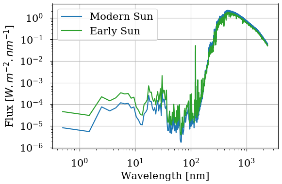
Figure 1 Stellar flux received by modern Earth computed for 0.0 Ga and 1.0 AU as well as stellar flux received by early Earth computed for 2.7 Ga and 1.0 AU from Claire et al. (2012).

The 1D version of the model uses a surface ocean, a surface mean albedo of 0.28, a mean solar zenith angle of 60^∘ and an eddy diffusion coefficient vertical profile from Zahnle et al. (2006).

Photochemical losses from the atmosphere by methane oxidation in the GCM are balanced with a production flux at the surface. This flux is established by fixing the abundance of the species considered in the first layer of the GCM (Eq. 3). It gathers all the surface contributions, such as organic carbon burial and input of reductants, which can be in dynamical equilibrium with atmospheric chemistry. When the stationary regime is reached, we can quantify the total photochemical loss and production of a species as its integrated surface flux required to maintain a constant surface abundance. Several simulations are performed on a grid of oxygen and methane abundance at the surface. The calculated fluxes are used to determine the photochemical loss flux as a function of the variable oxygen and methane abundances at the surface.

Gregory et al. (2021) suggested being cautious on the surface boundary conditions concerning a fixed mixing ratio or a fixed flux. While Gregory et al. (2021) do not describe the oxygen instability area with the fixed flux boundary condition, the fixed mixing ratio boundary condition allows us to explore the full equilibrium states. Fixing the flux is indeed more physical (or in this case biological) than fixing mixing ratios as the flux ratio can vary in time and space during evolution toward the steady state. But in the present study we wanted to intentionally determine the fluxes that correspond to a given steady-state composition. The resulting fluxes are finally consistent with a $\mathrm{1}/\mathrm{2}$ ratio driven by the oxygen and methane chemistry. Beyond this, additional simulations done by fixing the flux have shown some differences, which cannot fully be explained by the analysis of Gregory et al. (2021) considering the 3D geometry of the surface but the homogeneous boundary condition for each approach. This needs to be properly analyzed in a study focusing only on this aspect and could be done following this paper.

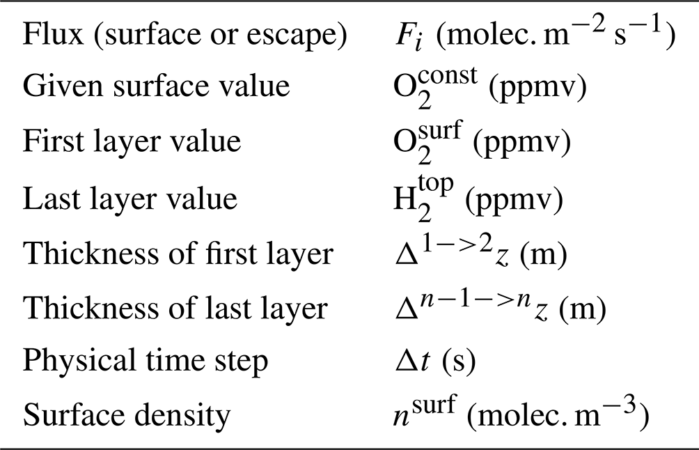
The GCM ensures the convergence of carbonaceous species by also fixing the CO₂ abundance at the surface to 1 %. In addition, the GCM takes into account atmospheric escape according to the Catling et al. (2001) model. The H₂ abundance in the last layer of the GCM is updated according to Eq. (1) thanks to the escape flux calculated by Eq. (2) (see corresponding terms in Table 1).

$$\begin{array}{}\text{(1)}& {\displaystyle }{\mathrm{H}}_{\mathrm{2}}^{\mathrm{top}}={\mathrm{H}}_{\mathrm{2}}^{\mathrm{top}}-{\displaystyle \frac{\mathrm{\Delta }t\times F_{{\mathrm{H}}_{\mathrm{2}}}}{{\mathrm{\Delta }}^{n-\mathrm{1}->n}z\times n^{\mathrm{top}}}}\text{(2)}& {\displaystyle }{F}_{{\mathrm{H}}_{\mathrm{2}}}=\mathrm{2.5}\times {\mathrm{10}}^{\mathrm{17}}\times \left({\mathrm{H}}_{\mathrm{2}}^{\mathrm{top}}+\mathrm{2}{{\mathrm{CH}}_{\mathrm{4}}}^{\mathrm{top}}+{{\mathrm{H}}_{\mathrm{2}}\mathrm{O}}^{\mathrm{top}}\right)\text{(3)}& {\displaystyle }{F}_{{\mathrm{O}}_{\mathrm{2}}}=\left({\mathrm{O}}_{\mathrm{2}}^{\mathrm{const}}-{\mathrm{O}}_{\mathrm{2}}^{\mathrm{surf}}\right){\displaystyle \frac{{\mathrm{\Delta }}^{\mathrm{1}->\mathrm{2}}z}{\mathrm{\Delta }t}}{n}^{\mathrm{surf}}\end{array}$$

Table 1 Terms used in Eqs. (1)–(3).

3 Methane oxidation fluxes

Atmospheric oxygen loss is dominated by the oxidation of methane as in Reaction (R2). The oxidation of methane is catalyzed by OH radicals (Gebauer et al., 2017). These radicals are produced by the photochemistry of water vapor.

$$\begin{array}{}\text{(R6)}& {\displaystyle }{\mathrm{H}}_{\mathrm{2}}\mathrm{O}+h\mathit{\nu }⟶\mathrm{OH}+\mathrm{H}\text{(R7)}& {\displaystyle }{\mathrm{H}}_{\mathrm{2}}\mathrm{O}+\mathrm{O}{(}^{\mathrm{1}}\mathrm{D})⟶\mathrm{OH}+\mathrm{OH}\end{array}$$

The amount of water vapor in the troposphere is controlled by temperature in a 1D model with an infinite water reservoir on the surface, but in a 3D dynamic model with dry continental surfaces, it also depends on the horizontal transport, evaporation and precipitation.

Photochemical processes depend on insolation and therefore on diurnal and seasonal variations. The formation of the ozone layer is a turning point for the photochemical balance. The ozone layer produces a UV shield, which limits the photochemical processes leading to methane oxidation and destroying oxygen. Oxygen can accumulate more efficiently and form more ozone. This positive feedback creates an oxygen instability which accounts for the sudden oxygenation of the atmosphere and may therefore be sensitive to the spatial distribution of ozone and thus to the global 3D transport.

In this section, we compare the results between the 1D and 3D model for photochemical oxygen and methane losses at steady state. We compute the variation of vertical chemical pathways to methane oxidation as a function of the surface O₂ fixed abundance. We also analyze the spatial distribution of ozone. Finally, we examine how surface fluxes required to sustain a steady state depend on surface temperature.

3.1 From 1D to 3D models

We ran the 1D model until steady state for a range of O₂ from 10⁻⁷ to 10⁻³ volume mixing ratio and CH₄ from 10⁻⁶ to 10⁻³ volume mixing ratio. Figure 2 shows the total atmospheric O₂ loss ($F_{{\mathrm{O}}_{\mathrm{2}}}$) as a function of these two parameters. These results are consistent with the previous study of Zahnle et al. (2006).

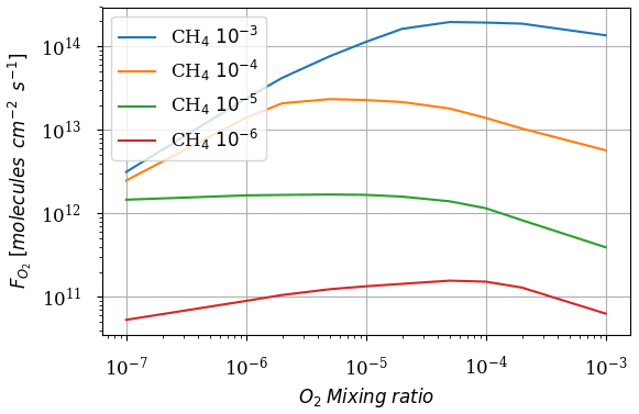
Figure 2 Oxygen atmospheric loss ($F_{{\mathrm{O}}_{\mathrm{2}}}$) as a function of surface O₂ for a surface CH₄ from 10⁻⁶ to 10⁻³.

Figure 3 shows the atmospheric losses of oxygen ($F_{{\mathrm{O}}_{\mathrm{2}}}$) and methane ($F_{{\mathrm{CH}}_{\mathrm{4}}}$), the hydrogen escape flux ($F_{{\mathrm{H}}_{\mathrm{2}}}$), and the ozone column density computed with the 1D and 3D version of the GCM for a methane abundance of 10⁻⁴ and an oxygen abundance grid between 10⁻⁷ and 10⁻³. The results are obtained after the convergence of the model with less than 1 % variation of the average of the last 50 time steps in 1D or the last year in 3D compared to the previous one. This is done for the H₂, CO₂, CH₄ and O₂ surface flux, the H₂, CO₂, CH₄, O₂ and O₃ column density, the surface temperature, the outgoing longwave radiation (OLR), and the absorbed shortwave radiation (ASR). The surface fluxes at steady state in 3D present horizontal and seasonal variations and are averaged over the planetary surface and over 1 year (500 d). Timescales of the rise of oxygen are much larger than a year, and the seasonal fluctuations are therefore not included in the following discussions. Discrepancies between 3D and 1D never exceed 10 % for $F_{{\mathrm{O}}_{\mathrm{2}}}$ and $F_{{\mathrm{CH}}_{\mathrm{4}}}$. However, the ozone column is always found to be larger in 1D: up to 5 times the mean column obtained with 3D. Other values of the arbitrary 1D zenith solar angle do not seem to explain this discrepancy. Figure 3 compares 1D simulations for both 40 and 60^∘, which present tiny differences compared to the 3D results. The average profiles of O₂, O₃, CO, CH₄, H₂ and water vapor found in 1D and 3D are presented in Fig. 4. Differences can come either from averaging the UV irradiation geometry in 1D or from horizontal and vertical transport. A priori, the photochemical losses ($F_{{\mathrm{O}}_{\mathrm{2}}}$ and $F_{{\mathrm{CH}}_{\mathrm{4}}}$) are not significantly modified (Fig. 3) and the vertical transport seems to be responsible for these differences. The 3D vertical transport seems to transport species more efficiently than the 1D transport model, which uses an eddy coefficient from Zahnle et al. (2006) to mimic the 3D transport. In particular, this results in smaller vertical gradients with the 3D model (Fig. 4).

Figure 3 Oxygen atmospheric loss ($F_{{\mathrm{O}}_{\mathrm{2}}}$), methane atmospheric loss ($F_{{\mathrm{CH}}_{\mathrm{4}}}$), hydrogen escape ($F_{{\mathrm{H}}_{\mathrm{2}}}$) and O₃ column density as a function of surface O₂ for a surface CH₄ set up at 10⁻⁴. Solid: results of the 3D model (averaged over the surface and a year). Dashed: 1D results at a zenith solar angle of 60^∘. Dotted: 1D results at a zenith solar angle of 40^∘.

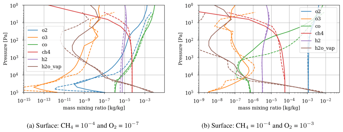
Figure 4 Species profile for 3D surface and annual average (solid) as well as the 1D (dashed) model.

Despite the aforementioned small departures, we find that the 1D model reproduces the results of the more comprehensive 3D model.

3.2 Vertical distribution of O₂ losses

At steady state (averaging seasonal variations) O₂ photochemical losses compensate for the surface outgassing of O₂. The ratio $\mathrm{1}/\mathrm{2}$ between $F_{{\mathrm{O}}_{\mathrm{2}}}$ and $F_{{\mathrm{CH}}_{\mathrm{4}}}$ (Fig. 3) shows that the atmospheric losses of oxygen and methane are dominated by the methane oxidation in Reaction (R2), which uses two molecules of O₂ for each molecule of methane (and forms one molecule of CO₂ and two molecules of H₂O). While oxygen molecules are mainly involved with the CO and CO₂ cycle (Gebauer et al., 2017), CH₄ is dominated by methane oxidation. The O₂, CO and CO₂ cycle is not a global loss of oxygen because there are no sources or losses of CO at the surface, and consequently O₂ has a null balance, contrary to methane oxidation. So, to analyze how losses of molecular oxygen are distributed in altitude, it is clearer to look at the methane loss, dominated by the oxidation of methane.

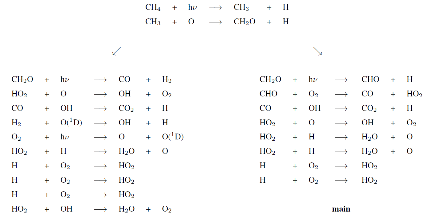
Figure 5 represents the rate of methane destruction as a function of altitude and for different O₂ levels. As for their integrated value, the vertical profiles of $F_{{\mathrm{O}}_{\mathrm{2}}}$ and $F_{{\mathrm{CH}}_{\mathrm{4}}}$ are similar when computed with 1D and 3D models. We distinguish the contribution to the loss of three main altitude domains: the troposphere, stratosphere and above. The losses are dominated, whatever the O₂ abundance, by the tropospheric contribution. In Appendix B, we empirically identify the main reaction pathways leading to a net methane oxidation (Reaction R2). Figure 5 shows a migration of losses from the troposphere to the stratosphere when oxygen abundance increases. Catalysis by OH remains at the heart of the oxidation mechanism, although a different reaction pathway is identified (Appendix B): as stratospheric ozone becomes more abundant, the production of O(¹D) through its photolysis increases:

$$\begin{array}{}\text{(R8)}& {\mathrm{O}}_{\mathrm{3}}+h\mathit{\nu }⟶{\mathrm{O}}_{\mathrm{2}}+\mathrm{O}{(}^{\mathrm{1}}\mathrm{D}),\end{array}$$

which then initiates the production of OH through Reaction (R7) instead of the O(¹D) coming from O₂ photolysis. The stratospheric contribution is less efficient than the tropospheric one, which is why $F_{{\mathrm{O}}_{\mathrm{2}}}$ decreases for high abundances of oxygen. Finally, there are CH₄ and O₂ losses in the upper atmosphere (around 10 Pa), which are less sensitive to the surface O₂ level. This contribution is no longer dominated by the catalysis of OH but comes from the photolysis of methane. The different pathways are identified in Appendix B. Due to the complexity of the chemistry, we developed suggested pathways which are relatively consistent with the work of Gebauer et al. (2017).

Figure 5 Methane photochemical losses as a function of altitude for several O₂ levels and a methane VMR of 10⁻⁴ at the surface. Solid: results of the 3D model (averaged over the surface and a year). Dashed: 1D results.

3.3 Ozone

Figure 6 shows how the ozone column density during a year varies with latitude from low to high pO₂. At low pO₂ we observe a maximum of ozone column density close to the poles during winter, while it switches to summer and lower latitudes (∼ 20^∘) at high pO₂. For comparison, we computed the ozone column density for the current Earth with and without continents. Our simulation of the current Earth with continents reproduces the present-day ozone distribution quite well (Tian et al., 2010), with a maximum close to the North Pole in March and at 50^∘S in October. The poleward transport of ozone in our simulation seems weaker than in reality, certainly due to the absence of the effect of gravity waves, which play a major role in the Brewer–Dobson circulation. By removing continents, the ozone maximum occurs later for both hemispheres, mostly due to the thermal inertia of the ocean. For such a case, the maximum of ozone occurs in the same season as the early Earth with high pCO₂ but at higher latitudes (∼ 45^∘). This is due to the faster rotation of the early Earth, limiting the latitudinal extension of the stratospheric circulation.

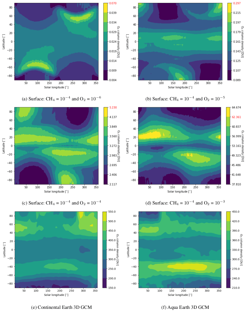
Figure 6 Ozone column density zonal mean over 13 years for early Earth as well as over 1 year for an actual simulated continental Earth and aqua Earth. 1D simulated early Earth values are highlighted in red.

The 3D effects have no significant consequence for the photochemical losses of O₂. The decrease in $F_{{\mathrm{O}}_{\mathrm{2}}}$ with increasing levels of O₂ above an O₂ volume mixing ratio (VMR) of 10⁻⁵ (Fig. 3) is due to the formation of the ozone layer due to UV shielding of methane oxidation (Goldblatt et al., 2006; Zahnle et al., 2006). Figure 6 shows latitudinal variations relatively less than a factor of 2, which have a tiny impact on the ozone lifetime and photochemistry, and Fig. 7 shows that ozone is relatively homogeneous over the whole planet, making 1D modeling relevant. Nevertheless, there are some variations of the O₃ column with latitude and related variations of the biologically harmful UV flux reaching the surface (Fig. 8). This nonhomogeneous opacity of the ozone UV shield may be important for the evolution and distribution of organisms living at the surface.

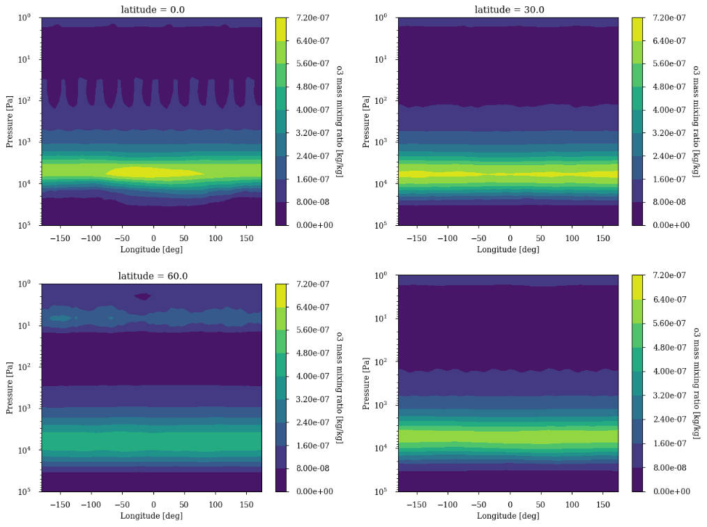
Figure 7 Ozone annual average longitudinal profile for latitudes 0, 30 and 60^∘ as well as the latitudinal average. Surface: CH₄ = 10⁻⁴ and O₂ = 10⁻³.

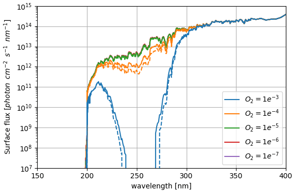
Figure 8 Stellar flux reaching the surface for several surface oxygen levels and surface methane of 10⁻⁴. Results of the 3D model surface and annual average (solid) as well as the 1D model (dashed).

3.4 Surface temperature effect

The resulting tropospheric temperature profile, calculated in both 1D and 3D models, follows a moist or dry adiabat that controls the vertical profile of water vapor, which, in turn, affects the greenhouse warming. Since this water vapor is the source of OH, which is a catalyzer of methane oxidation, this interplay suggests a possible link between surface temperature and photochemical losses of CH₄ and O₂, which we investigate here.

The previous results (Fig. 3) were obtained with a surface temperature close to 280 K, whatever the oxygen abundance at the surface, and an abundance of methane of 10⁻⁴. The surface temperature is the same because all the parameters are the same (rotation period, obliquity, solar input, surface composition – water or continent, continental albedo, etc.) and the main greenhouse gases (CO₂, CH₄) are not changed depending on the oxygen level.

As a first test to assess the effect of surface temperature, we use the 1D model with a surface temperature forced to remain at 220 K (by setting the heating and cooling rate of the surface to zero). This is the approximate surface temperature that would be reached by the 1D model with a frozen start, although the actual value would depend on the level of greenhouse CH₄. This way we can evaluate the impact of a snowball event on the photochemistry. Figure 9 shows that photochemical losses decrease with the temperature. How strong this decrease is depends on the O₂ level, with the drop being the largest around the maximum of $F_{{\mathrm{O}}_{\mathrm{2}}}$, so for a VMR of O₂ around 10⁻⁵. At this O₂ level, the photochemical losses occur entirely in the troposphere. Figure 10 compares the vertical profiles of methane photochemical losses for a surface temperature of 280 and 220 K as well as for different oxygen abundances at the surface. We see that the influence of surface temperature on the losses is located in the troposphere. Thus, the larger the tropospheric contribution, the larger the decrease in losses. The stratospheric thermal profile and the tropopause (the cold trap that controls the transport of water vapor to the stratosphere) show little response to a decrease in surface temperature from 280 to 220 K (see Fig. 13). As a consequence only the tropospheric chemistry is affected, as can be seen in the species profiles (Fig. 11).

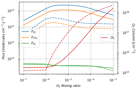
Figure 9 Surface oxygen ($F_{{\mathrm{O}}_{\mathrm{2}}}$) and methane ($F_{{\mathrm{CH}}_{\mathrm{4}}}$) fluxes, hydrogen escape ($F_{{\mathrm{H}}_{\mathrm{2}}}$), and O₃ column density as a function of surface O₂ for a surface CH₄ set up at 10⁻⁴. Results for a 1D model surface temperature of 280 K (solid) and 220 K (dashed).

Figure 10 Methane photochemical losses as a function of altitude for several O₂ levels and a surface CH₄ VMR of 10⁻⁴. Results from 1D modeling and for a surface temperature of 280 K (solid) and 220 K (dashed).

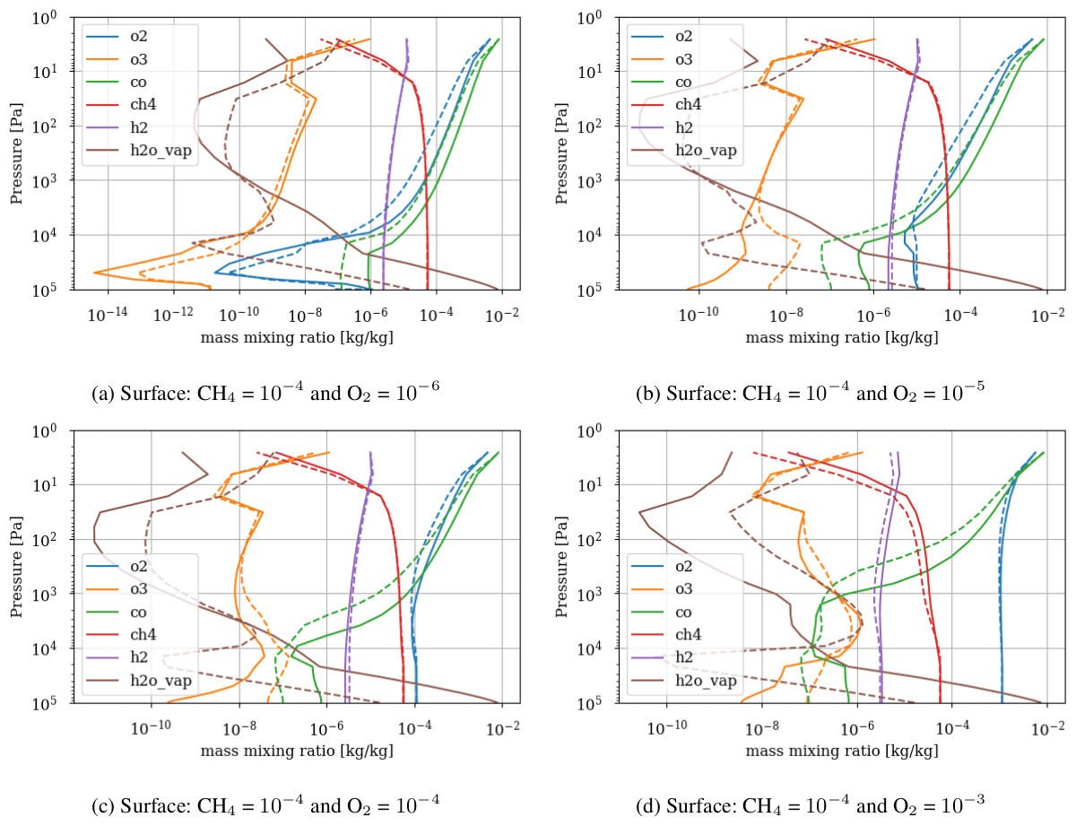
Figure 11 Species profile for a 1D model surface temperature of 280 K (solid) and 220 K (dashed).

The main implication of this result is that, under conditions of a global glaciation, the oxygen instability is triggered for an oxygen abundance or flux about an order of magnitude lower. For a given O₂ flux, glacial conditions should favor the switch from an oxygen-poor to an oxygen-rich atmosphere. During glaciations, however, environments able to provide both light and liquid water are considerably limited, making a considerable drop in the photosynthetic production of O₂ and the burial of biomass likely. To realistically simulate this feedback, one would need to couple the present model to a biogeochemical box model that simulated O₂ and CH₄ production.

The temperature trend of oxygen losses is determined. These losses are calculated using the 1D model by setting different surface temperatures for a methane abundance of 10⁻⁴ and an oxygen abundance of 10⁻⁵ at the surface. Figure 12 shows $F_{{\mathrm{CH}}_{\mathrm{4}}}$ (equivalent to $\mathrm{1}/\mathrm{2}$ $F_{{\mathrm{O}}_{\mathrm{2}}}$) as a function of surface temperature. We observe an order of magnitude increase in losses per 50 K. The discontinuity at 273 K is artificially produced by the change in albedo at the surface between ice-free oceans (albedo 0.07) and fully ice-covered oceans (albedo 0.65). The increase in albedo below 273 K reflects more UV flux and increases photochemical losses in the troposphere. The 3D model smooths this effect by gradually freezing the ocean at the surface. We use the slow convergence of the 3D model towards a frozen state. The photochemical equilibrium is established on a timescale of a few years, whereas the progressive freezing of the surface takes place over several decades. A quasi-stationary state of species abundance in the atmosphere and consequently of atmospheric losses is rapidly established. During freezing on a longer timescale, the evolution of temperature and oxygen losses in their quasi-stationary state is recorded to establish the link between oxygen losses and temperature; see Fig. 12. The 3D model converges to a frozen state wherein the sea ice extends from the poles to 20–25^∘ N and S. The coverage is about 60 %–65 %, as observed in Charnay et al. (2013), and the surface temperature converges to 230 K. A cold start with a completely frozen surface is then performed to evaluate the impact of the 3D model following a global glaciation. The results in Fig. 12 show that in addition to the smoothing of the albedo effect, the trend is weaker than the 1D model. At the root of this difference is the difference in transport between the two models. The 3D model mixes the tropospheric temperature more efficiently, warming the troposphere and reducing the impact of a cooling on atmospheric losses; see Fig. 13.

Figure 12 $F_{{\mathrm{CH}}_{\mathrm{4}}}$ depending on the surface temperature. Results of the 3D model surface and annual average (solid and mark for snowball) as well as the 1D model (dashed). Surface: CH₄ = 10⁻⁴ and O₂ = 10⁻⁵.

Figure 13 Temperature profile for a surface temperature of 280 and 260 K. Results of the 3D model surface and annual average (solid) as well as the 1D model (dashed).

Temperature appears to have a significant impact on atmospheric loss. Between a temperate state and an ice age, oxygen losses can vary by a factor of 2 to 4. Oxygen abundance and methane abundance can accumulate more in the atmosphere during an ice age. The consequences of ice ages for the temporal evolution of oxygen and methane during the GOE are studied in the following by considering this new trend.

4 Temporal evolution, overshoot and glaciation events

After the GOE, a carbon-13 isotopic variation of nearly 15 ‰ is observed (Lyons et al., 2014). This event is called the Lomagundi event (Bachan and Kump, 2015). Although the dynamics of the oxygenation process remain uncertain, this event suggests an over-oxygenation of the atmosphere (Catling and Zahnle, 2020). Other evidence supports this phenomenon, such as the evolution of the δ³⁴S fraction of carbonate-associated sulfates (Planavsky et al., 2012; Schröder et al., 2008) and fluctuations in the degree of uranium enrichment in organic-rich shales (Partin et al., 2013). An increase in overall oxygen productivity followed by a decrease would seem to account for this over-oxygenation (Harada et al., 2015; Holland and Bekker, 2012; Hodgskiss et al., 2019). Nevertheless, we have previously seen that a global glaciation phenomenon can significantly decrease the atmospheric oxygen losses. It is therefore not impossible that Huronian glaciations could also have had an impact on atmospheric over-oxygenation during the global oxygenation process. In order to study the dynamics of over-oxygenation, a time evolution equation model is established based on the equations of Goldblatt et al. (2006) and Claire et al. (2006) and adjusted to take into account variations in primary oxygen productivity and atmospheric losses. We compare the previous Goldblatt et al. (2006) parameterization for atmospheric loss with the GCM interpolated function for the time evolution without an over-oxygenation using the time evolution equation model established. We then apply this model to reproduce the over-oxygenation and the fluctuations brought by glaciations.

4.1 Equation model

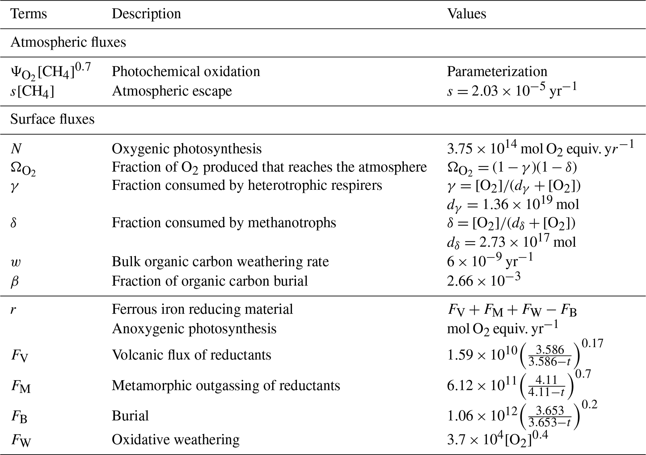
The temporal evolution of oxygen and methane abundance during the GOE is modeled by the Goldblatt et al. (2006) equations. They relate atmospheric losses, described in Sect. 3, to surface contributions associated with biogeochemical exchanges. Goldblatt et al. (2006) propose for this biosphere model a parameterization of atmospheric losses according to ${\mathrm{\Psi }}_{{\mathrm{O}}_{\mathrm{2}}}[{\mathrm{CH}}_{\mathrm{4}}{]}^{\mathrm{0.7}}$, where ${\mathrm{\Psi }}_{{\mathrm{O}}_{\mathrm{2}}}={\mathrm{10}}^{a_{\mathrm{1}}{\mathit{\psi }}^{\mathrm{4}}+a_{\mathrm{2}}{\mathit{\psi }}^{\mathrm{3}}+a_{\mathrm{3}}{\mathit{\psi }}^{\mathrm{2}}+a_{\mathrm{4}}\mathit{\psi }+a_{\mathrm{5}}}$, ψ=log ([O₂]), a₁=0.0030, $a_{\mathrm{2}}=-\mathrm{0.1655}$, a₃=3.2305, $a_{\mathrm{4}}=-\mathrm{25.8343}$ and a₅=71.5398. Goldblatt et al. (2006) also estimate the value of the different parameters (see Table 2). A set of values is associated with a steady state of oxygen and methane abundances. Depending on the value of the flux of reductant r, one is in a state of oxygen-poor or oxygen-rich equilibrium. In order to study the temporal evolution between these two equilibrium states, we use the results of Claire et al. (2006) to establish a temporal evolution of the flux of reductant r (Fig. 14). We introduce this temporal evolution in the equations of Goldblatt et al. (2006) to reproduce the dynamics of oxygenation. Finally, we introduce a coefficient α_N (≥ 1) to model photosynthetic over-productivity responsible for the over-oxygenation, as well as a coefficient α_Ψ (≤ 1) to model the decrease in atmospheric losses during a glaciation. The evolution of the abundance of oxygen, methane and buried carbon is then described by the following equations:

$$\begin{array}{}\text{(4)}& {\displaystyle }\begin{array}{rl}{\displaystyle \frac{\mathrm{d}\left[{\mathrm{CH}}_{\mathrm{4}}\right]}{\mathrm{d}t}}& ={\mathit{\alpha }}_N{\displaystyle \frac{\mathrm{1}}{\mathrm{2}}}{\mathrm{\Omega }}_{{\mathrm{O}}_{\mathrm{2}}}N+{\displaystyle \frac{\mathrm{1}}{\mathrm{2}}}{\mathrm{\Omega }}_{{\mathrm{O}}_{\mathrm{2}}}r-s\left[{\mathrm{CH}}_{\mathrm{4}}\right]\\ & -{\mathit{\alpha }}_{\mathrm{\Psi }}{\displaystyle \frac{\mathrm{1}}{\mathrm{2}}}{\mathrm{\Psi }}_{{\mathrm{O}}_{\mathrm{2}}}[{\mathrm{CH}}_{\mathrm{4}}{]}^{\mathrm{0.7}}-{\displaystyle \frac{\mathrm{1}}{\mathrm{2}}}{\mathrm{\Omega }}_{{\mathrm{O}}_{\mathrm{2}}}(\mathit{\beta }(N+r)-w\mathrm{C}),\end{array}\text{(5)}& {\displaystyle }\begin{array}{rl}{\displaystyle \frac{\mathrm{d}\left[{\mathrm{O}}_{\mathrm{2}}\right]}{\mathrm{d}t}}& ={\mathit{\alpha }}_N{\mathrm{\Omega }}_{{\mathrm{O}}_{\mathrm{2}}}N-\left(\mathrm{1}-{\mathrm{\Omega }}_{{\mathrm{O}}_{\mathrm{2}}}\right)r-s\left[{\mathrm{CH}}_{\mathrm{4}}\right]\\ & -{\mathit{\alpha }}_{\mathrm{\Psi }}{\mathrm{\Psi }}_{{\mathrm{O}}_{\mathrm{2}}}[{\mathrm{CH}}_{\mathrm{4}}{]}^{\mathrm{0.7}}-\left(\mathrm{1}-{\mathrm{\Omega }}_{{\mathrm{O}}_{\mathrm{2}}}\right)(\mathit{\beta }(N+r)-w\mathrm{C}),\end{array}\text{(6)}& {\displaystyle \frac{\mathrm{d}C}{\mathrm{d}t}}=\mathit{\beta }(N+r)-w\mathrm{C},\end{array}$$

with the different terms and values detailed in Table 2.

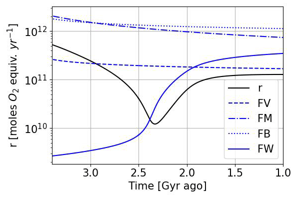
Figure 14 Temporal evolution of the reductant contributions (see Table 2) with α_i = 1 and using the Goldblatt et al. (2006) parameterization for oxygen atmospheric loss ($F_{{\mathrm{O}}_{\mathrm{2}}}$).

Table 2 Equation dependencies and values from Goldblatt et al. (2006). Reductant model from Claire et al. (2006) with time t (Gyr) and amount of oxygen [O₂] (mol).

The size and shape of the over-oxygenation are uncertain, as are the possible variations in oxygen sources and losses during this process. We then arbitrarily define a log-polynomial fit for the time evolution of the parameters ${\mathit{\alpha }}_i=e^{\left(a\right(t-t_{\mathrm{0}}{)}^{\mathrm{2}p}+b)}$ (α_i=α_N or α_Ψ). When there is no deviation from the initial model the values of α_i are equal to 1. The variation of the α_i parameters is triggered in a way that is consistent with the predictions of previous studies on the evolution of primary productivity and ice ages.

4.2 Dynamics with constant temperature and constant primary productivity

The Goldblatt et al. (2006) parameterization for atmospheric oxygen loss as a function of oxygen and methane abundance is compared (Fig. 15) to the results obtained with the 1D GCM, which are shown to be similar to the 3D model. The parameterization established by Goldblatt et al. (2006) does not seem to correctly capture the methane dependence. This variation is not independent of oxygen abundance and cannot be described by a constant power x of methane abundance [CH₄]^x. At high oxygen abundances ($>{\mathrm{10}}^{-\mathrm{4}}$) the variation seems to increase with increasing methane and conversely at lower oxygen abundances ($<{\mathrm{10}}^{-\mathrm{4}}$). An asymptote appears to emerge at low oxygen abundances for the highest methane abundances ($>{\mathrm{10}}^{-\mathrm{5}}$). This behavior has already been seen in Zahnle et al. (2006).

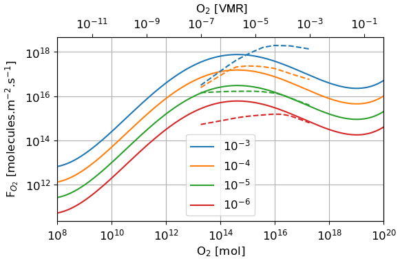
Figure 15 Oxygen atmospheric loss ($F_{{\mathrm{O}}_{\mathrm{2}}}$) depending on oxygen and methane; labeled in VMR. Goldblatt et al. (2006) parameterization (solid) and GCM 1D results (dashed).

Figure 16 shows the equilibrium states as a function of the total reductant parameter r with the Goldblatt et al. (2006) parameterization and an interpolation of the 1D GCM results for the atmospheric losses. These curves show the stable and unstable equilibrium states of the atmosphere. They justify the rapid switch from an oxygen-poor to an oxygen-rich state. The flux of reductant that triggers the instability varies from about 1 × 10¹⁰ to 3 × 10¹⁰ mol O₂ equiv. yr⁻¹ with the interpolation of the 1D GCM results. The asymptotic behavior of the atmospheric losses calculated with the 1D GCM at low oxygen and high methane (high r) levels can be seen in the equilibrium states with an approximately constant value at those levels. This behavior remains uncertain.

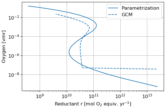
Figure 16 Equilibrium states of the time evolution equation model depending on the reductant parameter r. Oxygen atmospheric loss ($F_{{\mathrm{O}}_{\mathrm{2}}}$) Goldblatt et al. (2006) parameterization (solid) and GCM 1D results (dashed).

A time evolution of oxygen and methane abundance with these two atmospheric loss models (Fig. 17) shows that with the interpolation of 1D GCM results oxygenation is faster. The equilibrium positions in Fig. 16 show that indeed the amount of oxygen is more sensitive to the flux of reductant. Oxygenation therefore occurs for a smaller variation of the reductant flux. As the methane abundance is directly related to the reductant flux ([CH₄] = $r/s$), we also observe a smaller variation of the methane abundance during oxygenation.

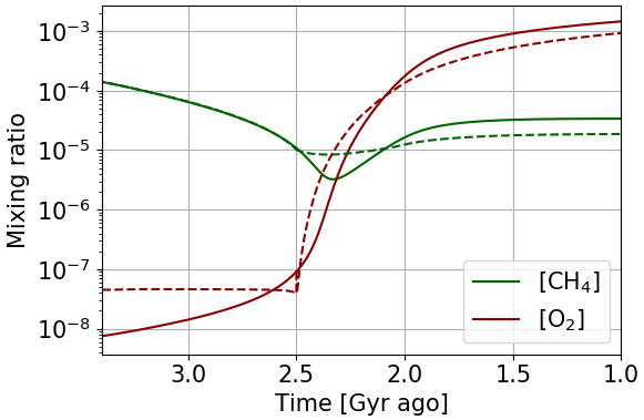
Figure 17 Temporal evolution of oxygen and methane with α_i = 1. Oxygen atmospheric loss ($F_{{\mathrm{O}}_{\mathrm{2}}}$) Goldblatt et al. (2006) parameterization (solid) and GCM 1D results (dashed).

4.3 Long overshoot with variable primary productivity

We model a long variation over 400 million years of the primary productivity, parameter α_N, with a first phase of overproduction before a return to the initial production. We represent in Fig. 18 the reference evolution for constant α_N equal to 1, as well as two different intensities of over-productivity with a maximum at 2 and 10 times the initial productivity. The reference model is in good agreement with the results of Goldblatt et al. (2006) and Claire et al. (2006). We observe a variable over-oxygenation depending on the intensity of the primary productivity variation, but also an overabundance of methane. The primary productivity corresponds to photosynthetic production of oxygen but also of organic matter, transformed into methane by the methanogens. Consequently, the production of methane is increased in addition to that of oxygen. Such an overabundance of methane is not highlighted by previous studies or by the geological record. It is difficult to constrain the amount of methane at that time. This scenario is therefore possible, although one could also imagine that oxygen enrichment of the atmosphere limited the conversion of organic matter into methane: a conversion that is carried out by methanogens, developing more favorably in a reducing environment. A similar explanation has been proposed for the debated higher level of methane during the Boring Billion periods at 1.8–0.8 Ga (Pavlov et al., 2003).

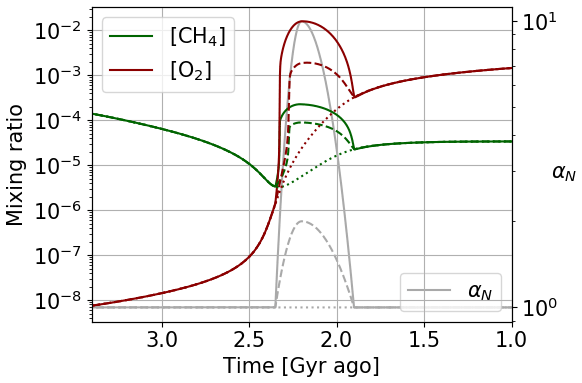
Figure 18 Oxygen and methane temporal evolution. Models with α_N constant equalling 1, reaching a factor of 2 and reaching a factor of 10.

This temporal evolution is identical if we model an inverse variation of atmospheric losses (${\mathit{\alpha }}_{\mathrm{\Psi }}=\mathrm{1}/{\mathit{\alpha }}_N$), corresponding to a glaciation event of 400 million years. This scenario is less likely since there are several shorter glaciation events called Huronian glaciations (Young et al., 2001). In addition, a change in primary productivity provides a link to the positive anomaly in carbon-13 isotope fractionation (Lyons et al., 2014). By using the model of the evolution of the isotopic ratio of Goldblatt et al. (2006), we can evaluate the impact of the variation of primary productivity or atmospheric losses on this ratio:

$$\begin{array}{}\text{(7)}& f={\displaystyle \frac{{\mathit{\delta }}_{\mathrm{carb}}-{\mathit{\delta }}_i}{{\mathit{\delta }}_{\mathrm{carb}}-{\mathit{\delta }}_{\mathrm{org}}}},\end{array}$$

where f is the fraction of buried volcanic carbon, δ_carb is the carbon-13 isotope ratio δ¹³C for carbonates, δ_i is the carbon-13 isotope ratio δ¹³C for volcanic carbon, and δ_org is the carbon-13 isotope ratio δ¹³C for organic carbon. The fraction of buried volcanic carbon can be described by the biosphere model based on the fraction C​​​​​​​ of buried carbon, where C ∼ $\frac{\mathit{\beta }}{w}(N+r)$. We establish the approximation that f α(N+r). Goldblatt et al. (2006) define the initial state during the Archean with δ_carb = 0 ‰, δ_i = −6 ‰ and δ_org = −30 ‰, giving f = 0.2. With this initial state, we determine the relation of proportionality between f and (N+r), and then we evaluate the evolution of the isotopic fractionation of the carbonates δ_carb during the temporal evolution of the oxygen and methane abundance thanks to the following formula.

$$\begin{array}{}\text{(8)}& {\mathit{\delta }}_{\mathrm{carb}}={\displaystyle \frac{{\mathit{\delta }}_i-f\times {\mathit{\delta }}_{\mathrm{org}}}{\mathrm{1}-f}}\end{array}$$

Figure 19 represents the evolution of δ_carb as a function of time for the time evolution models established with primary over-productivity reaching a factor of 2 and the inverse evolution of atmospheric losses. Primary over-productivity is consistent with the anomaly of about 15 ‰ measured in contrast to the decrease in atmospheric losses.

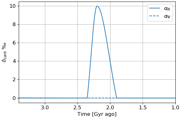
Figure 19 Temporal evolution of δ_carb. Models with α_N reaching a factor of 2 and α_Ψ reaching a factor of 0.5.

4.4 Short overshoot with variable temperature

The Huronian glaciations represent several glacial events that took place during the oxygenation of the atmosphere at the beginning of the Proterozoic. The model of the α_Ψ parameter variation over 400 million years is therefore not consistent with the episodic nature of these glaciations. To reflect the impact of these glaciations on atmospheric losses, an episodic variation over shorter times during the oxygenation period can be established. Figure 20 presents the temporal evolution of oxygen and methane following this adjustment. We observe the punctual over-oxygenations linked to the variations of α_Ψ with a global trend that follows the temporal evolution of the initial model wherein α_i = 1. We note, during the over-oxygenation, an increase in the methane abundance. This increase in greenhouse gases can trigger the thawing of the surface. During the thawing, the surface temperature increases, causing an increase in atmospheric losses by oxidation of methane. This is why the amount of methane decreases again. This negative feedback, coupled with the hysteresis phenomenon between the frozen and warm state of the surface, could be one of the key factors to explain the cyclic character of Huronian glaciations.

Figure 20 Oxygen and methane temporal evolution. Models with α_Ψ reaching a factor of 0.1 on shorter timescales.

Figure 21 shows the complete model for over-oxygenation with a 400-million-year variation in primary productivity and a maximum factor of 2, as well as a fluctuation provided by shorter timescale variations in atmospheric losses due to Huronian glaciations with a maximum factor of 0.5. This coupling is not intended to exactly reproduce what happened during the GOE but to highlight both effects on the evolution of oxygen and methane during this event.

Figure 21 Oxygen and methane temporal evolution. Models with α_N reaching a factor of 2. Models with α_Ψ reaching a factor of 0.5 on shorter timescales.

5 Summary

The atmospheric equilibrium states during the Archean and the Proterozoic have been established for the first time using a 3D photochemical–climate model. Despite some 3D transport discrepancies the atmospheric–surface equilibrium fluxes of methane and oxygen are not significantly different from a 1D model, as has been done in Zahnle et al. (2006) and Gebauer et al. (2017). Following, the (photo)chemical equilibrium pathways have been determined depending on the altitude. It highlights the evolution of the tropospheric and stratospheric contribution depending on the oxygen levels. What remains constant, however, is the important link with the OH molecules, which catalyze the methane oxidation. Because of that, we found a crucial dependency of the surface flux equilibrium with the surface temperature. This temperature dependence is sensitive to the 3D transport and appears weaker in 3D than in 1D. However, a global glaciation could reduce the oxygen atmospheric losses by a factor of 2 to 10. Taking this new contribution into account in a time evolution model, we show that glaciations bring fluctuations in oxygen and methane abundance with an overshoot during glaciations. The increase in methane following glaciation produces an additional greenhouse effect that could eventually lead to deglaciation. This warming increases the atmospheric losses of methane again, and it is possible to establish a cycle of glaciation–deglaciation. Little evidence of methane (Lowe and Tice, 2004; Cadeau et al., 2020) has yet been discovered, but it could explain how the planet has been warmed up enough to terminate the glaciation thanks to the methane greenhouse effect. The feedback between the glaciation and methane evolution coupled with the glaciation hysteresis process might also explain the multiple glaciations known as the Huronian glaciations. More generally, the link between temperature and photochemical processes shows that a decrease in temperature favors the oxygenation of the atmosphere. Without falling into a global glaciation, phenomena such as a decrease in atmospheric CO₂ or the emergence of continents induce a decrease in temperature favorable to the oxygenation of the atmosphere.

6 Perspectives

Beyond the temperature, the UV–visible stellar radiation received by the planet controls the photochemical processes and quantity of ozone that are essential for the oxygenation phenomenon of the atmosphere. A red dwarf such as TRAPPIST-1a presents a spectral distribution in favor of UV radiation with respect to visible radiation, which favors the accumulation of ozone. The 1D study of Gebauer et al. (2018) shows that around such red dwarfs the oxygenation of the atmosphere is triggered for lower atmospheric oxygen levels and surface oxygen flux. These irradiation conditions then favor the oxygenation of the atmosphere. A compact system such as TRAPPIST-1 presumably has synchronous planets (Vinson and Hansen, 2017), which creates interest in using 3D models. The permanent dichotomy between day and night side brings an important variation of temperature (Leconte et al., 2013) and photochemical processes. Red dwarfs represent the majority of the stars and would thus shelter the majority of the planets. It is then necessary to understand how an oxygenated atmosphere could evolve around these planets. For this, 3D models will be necessary to capture the effect of synchronization.

Appendix A: Chemical network

Ogawa and Ogawa (1975)Lewis et al. (1983)Gibson et al. (1983)Minschwaner et al. (1992)Yoshino et al. (1988)Fally et al. (2000)Chan et al. (1993)Stark et al. (2007)Yoshino et al. (1996)Parkinson et al. (2003)Lewis and Carver (1983)Sander et al. (2006)Mota et al. (2005)Chung et al. (2001)Thompson et al. (1963)Schurgers and Welge (1968)Demore et al. (1997)Sander et al. (2003)Kameta et al. (2002)Chen and Wu (2004)Lee et al. (2001)Sander et al. (2011)Lee et al. (2001)Kasting et al. (1983)Chen et al. (1991)Smith et al. (1991)Laufer and Keller (1971)Sander et al. (2006)Sander et al. (2006)Sander et al. (2006)Ashfold et al. (1981)Campbell and Gray (1973)Sander et al. (2006)Sander et al. (2003)Christensen et al. (2002)Sander et al. (2011)Baulch et al. (2005)Banyard et al. (1980)Laufer (1981)Fahr et al. (1991)Friedrichs et al. (2002)Wagner and Wardlaw (1988)Wang et al. (2003)Sander et al. (2003)Sander et al. (2003)Sander et al. (2006)Sander et al. (2011)Sander et al. (2003)Sander et al. (2003)Sander et al. (2003)Sander et al. (2003)Sander et al. (2003)Sander et al. (2003)Sander et al. (2011)Sander et al. (2003)Sander et al. (2006)Sander et al. (2006)Sander et al. (2006)Sander et al. (2003)Sander et al. (2006)Sander et al. (2006)Sander et al. (2011)Sander et al. (2003)Sander et al. (2003)Sander et al. (2003)Tsang and Hampson (1986)Joshi and Wang (2006)Zahnle (1986)Donovan and Husain (1970)Giguere and Huebner (1978)Pitts et al. (1982)Pitts et al. (1982)Prasad and Huntress (1980)Baughcum and Oldenborg (1983)Stephens et al. (1988)Lander et al. (1990)Allen et al. (1992)Tsang and Hampson (1986)Stephens et al. (1988)Allen et al. (1992)Zahnle (1986)Brown and Laufer (1982)Romani et al. (1993)Zahnle (1986)Perry and Williamson (1982)Hampson and Garvin (1977)Fahr et al. (1991)Tsang and Hampson (1986)Warnatz (1984)Allen et al. (1992)Hoyermann et al. (1981)Benson and Haugen (1967)Hampson and Garvin (1977)Hampson and Garvin (1977)Berman et al. (1982)Becker et al. (1989)Zabarnick et al. (1986)Romani et al. (1993)Messing et al. (1981)Butler et al. (1981)Romani et al. (1993)Böhland et al. (1985)Zahnle (1986)Romani et al. (1993)Tsang and Hampson (1986)Ashfold et al. (1981)Tsang and Hampson (1986)Tsang and Hampson (1986)Yung et al. (1984)Darwin and Moore (1995)Zabarnick et al. (1986)Gladstone (1983)Huebner and Giguere (1980)Homann and Schweinfurth (1981)Huebner and Giguere (1980)Baulch et al. (1994)Tsang and Hampson (1986)Michael et al. (1979)Lee (1980)Miller et al. (1982)Watkins and Word (1974)Baulch et al. (1994)Baulch et al. (1994)Tsang and Hampson (1986)Sander et al. (2006)Sander et al. (2006)Sander et al. (2006)Sander et al. (2006)Jasper et al. (2007)Fenimore (1969)Adachi et al. (1981)Adachi et al. (1981)Zahnle (1986)Zahnle (1986)Wen et al. (1989)Tsang and Hampson (1986)Sander et al. (2006)Baulch et al. (1994)Baulch et al. (1992)Baulch et al. (1994)Sander et al. (2006)Sander et al. (2006)Wen et al. (1989)Sander et al. (2006)Tsang and Hampson (1986)Hampson and Garvin (1977)Tsang and Hampson (1986)

Table A1 Chemical network with rate coefficients and references used to model the early Earth. Units are per second (s⁻¹) for photolysis reactions, cubic centimeters per second (cm³ s⁻¹) for two-body reactions and centimeters to the power of six per second for three-body reactions. [M] correspond to the density in molecules per cubic centimeter (molec. cm⁻³). If k₀ and k_∞ are specified, the formula is $\frac{k_{\mathrm{0}}\left[M\right]}{\mathrm{1}+\frac{k_{\mathrm{0}}}{k_{\mathrm{\infty }}}\left[M\right]}{\mathrm{0.6}}^{{\left[\mathrm{1}+{\left[{\log }_{\mathrm{10}}\left(\frac{k_{\mathrm{0}}}{k_{\mathrm{\infty }}}\left[M\right]\right)\right]}^{\mathrm{2}}\right]}^{-\mathrm{1}}}$. If k_1a,0, k_1b,0, k_1a,∞ and F_c are specified, the formula is $k_{\mathrm{1}a,\mathrm{0}}\frac{\mathrm{1}+\frac{k_{\mathrm{1}b,\mathrm{0}}}{k_{\mathrm{1}a,\mathrm{\infty }}-k_{\mathrm{1}b,\mathrm{0}}}}{\mathrm{1}+\frac{k_{\mathrm{1}a,\mathrm{0}}}{k_{\mathrm{1}a,\mathrm{\infty }}-k_{\mathrm{1}b,\mathrm{0}}}}{F}_c^{{\left[\mathrm{1}+{\left[\log \left(\frac{k_{\mathrm{1}a,\mathrm{0}}}{k_{\mathrm{1}a,\mathrm{\infty }}-k_{\mathrm{1}b,\mathrm{0}}}\right)\right]}^{\mathrm{2}}\right]}^{-\mathrm{1}}}+k_{\mathrm{1}b,\mathrm{0}}\frac{\mathrm{1}}{\mathrm{1}+\frac{k_{\mathrm{1}a,\mathrm{0}}}{k_{\mathrm{1}a,\mathrm{\infty }}-k_{\mathrm{1}b,\mathrm{0}}}}{F}_c^{{\left[\mathrm{1}+{\left[\log \left(\frac{k_{\mathrm{1}a,\mathrm{0}}}{k_{\mathrm{1}a,\mathrm{\infty }}-k_{\mathrm{1}b,\mathrm{0}}}\right)\right]}^{\mathrm{2}}\right]}^{-\mathrm{1}}}$.

Appendix B: Methane oxidation pathways

Bilan

$$\begin{array}{}\text{(BR1)}& {\mathrm{CH}}_{\mathrm{4}}+\mathrm{2}{\mathrm{O}}_{\mathrm{2}}⟶{\mathrm{CO}}_{\mathrm{2}}+\mathrm{2}{\mathrm{H}}_{\mathrm{2}}\mathrm{O}\end{array}$$

Tropospheric dominant pathways

Stratospheric dominant pathway

$$\begin{array}{c}{\displaystyle }{\mathrm{CH}}_{\mathrm{4}}+\mathrm{OH}⟶{\mathrm{CH}}_{\mathrm{3}}+{\mathrm{H}}_{\mathrm{2}}\mathrm{O}\\ {\displaystyle }{\mathrm{CH}}_{\mathrm{3}}+{\mathrm{O}}_{\mathrm{2}}⟶{\mathrm{CH}}_{\mathrm{2}}\mathrm{O}+\mathrm{OH}\\ {\displaystyle }{\mathrm{CH}}_{\mathrm{2}}\mathrm{O}+\mathrm{OH}⟶\mathrm{CHO}+{\mathrm{H}}_{\mathrm{2}}\mathrm{O}\\ {\displaystyle }\mathrm{CHO}+{\mathrm{O}}_{\mathrm{2}}⟶\mathrm{CO}+{\mathrm{HO}}_{\mathrm{2}}\\ {\displaystyle }\mathrm{CO}+\mathrm{OH}⟶{\mathrm{CO}}_{\mathrm{2}}+\mathrm{H}\\ {\displaystyle }{\mathrm{HO}}_{\mathrm{2}}+\mathrm{O}⟶\mathrm{OH}+{\mathrm{O}}_{\mathrm{2}}\\ {\displaystyle }\mathrm{H}+{\mathrm{O}}_{\mathrm{2}}⟶{\mathrm{HO}}_{\mathrm{2}}\\ {\displaystyle }{\mathrm{HO}}_{\mathrm{2}}+h\mathit{\nu }⟶\mathrm{OH}+\mathrm{O}\end{array}$$

Upper atmosphere dominant pathway

$$\begin{array}{c}{\displaystyle }{\mathrm{CH}}_{\mathrm{4}}+h\mathit{\nu }⟶{}^{\mathrm{1}}{\mathrm{CH}}_{\mathrm{2}}+{\mathrm{H}}_{\mathrm{2}}\\ {\displaystyle }{}^{\mathrm{1}}{\mathrm{CH}}_{\mathrm{2}}+{\mathrm{O}}_{\mathrm{2}}⟶\mathrm{CHO}+\mathrm{OH}\\ {\displaystyle }\mathrm{CHO}+{\mathrm{O}}_{\mathrm{2}}⟶\mathrm{CO}+{\mathrm{HO}}_{\mathrm{2}}\\ {\displaystyle }\mathrm{CO}+\mathrm{OH}⟶{\mathrm{CO}}_{\mathrm{2}}+\mathrm{H}\\ {\displaystyle }{\mathrm{HO}}_{\mathrm{2}}+\mathrm{O}⟶\mathrm{OH}+{\mathrm{O}}_{\mathrm{2}}\\ {\displaystyle }{\mathrm{H}}_{\mathrm{2}}+\mathrm{O}{(}^{\mathrm{1}}\mathrm{D})⟶\mathrm{OH}+\mathrm{H}\\ {\displaystyle }{\mathrm{O}}_{\mathrm{2}}+h\mathit{\nu }⟶\mathrm{O}+\mathrm{O}{(}^{\mathrm{1}}\mathrm{D})\\ {\displaystyle }\mathrm{H}+{\mathrm{O}}_{\mathrm{2}}⟶{\mathrm{HO}}_{\mathrm{2}}\\ {\displaystyle }\mathrm{H}+{\mathrm{O}}_{\mathrm{2}}⟶{\mathrm{HO}}_{\mathrm{2}}\\ {\displaystyle }{\mathrm{HO}}_{\mathrm{2}}+\mathrm{OH}⟶{\mathrm{H}}_{\mathrm{2}}\mathrm{O}+{\mathrm{O}}_{\mathrm{2}}\\ {\displaystyle }{\mathrm{HO}}_{\mathrm{2}}+\mathrm{OH}⟶{\mathrm{H}}_{\mathrm{2}}\mathrm{O}+{\mathrm{O}}_{\mathrm{2}}\end{array}$$

Upper atmosphere secondary pathways (lower half)

Upper atmosphere secondary pathways (upper half)