the Creative Commons Attribution 4.0 License.
the Creative Commons Attribution 4.0 License.
 | 14 Jan 2022
Glacier response to Holocene warmth inferred from in situ 10Be and 14C bedrock analyses in Steingletscher's forefield (central Swiss Alps)
Irene Schimmelpfennig
Joerg M. Schaefer
Jennifer Lamp
Vincent Godard
Roseanne Schwartz
Edouard Bard
Thibaut Tuna
Naki Akçar
Christian Schlüchter
Susan Zimmerman
Mid-latitude mountain glaciers are sensitive to local summer temperature changes. Chronologies of past glacier fluctuations based on the investigation of glacial landforms therefore allow for a better understanding of natural climate variability at local scale, which is relevant for the assessment of the ongoing anthropogenic climate warming. In this study, we focus on the Holocene, the current interglacial of the last 11 700 years, which remains a matter of dispute regarding its temperature evolution and underlying driving mechanisms. In particular, the nature and significance of the transition from the early to mid-Holocene and of the Holocene Thermal Maximum (HTM) are still debated. Here, we apply an emerging approach by combining in situ cosmogenic 10Be moraine and 10Be–14C bedrock dating from the same site, the forefield of Steingletscher (European Alps), and reconstruct the glacier's millennial recession and advance periods. The results suggest that, subsequent to the final deglaciation at ∼10 ka, the glacier was similar to or smaller than its 2000 CE extent for ∼7 kyr. At ∼3 ka, Steingletscher advanced to an extent slightly outside the maximum Little Ice Age (LIA) position and until the 19th century experienced sizes that were mainly confined between the LIA and 2000 CE extents. These findings agree with existing Holocene glacier chronologies and proxy records of summer temperatures in the Alps, suggesting that glaciers throughout the region were similar to or even smaller than their 2000 CE extent for most of the early and mid-Holocene. Although glaciers in the Alps are currently far from equilibrium with the accelerating anthropogenic warming, thus hindering a simple comparison of summer temperatures associated with modern and paleo-glacier sizes, our findings imply that the summer temperatures during most of the Holocene, including the HTM, were similar to those at the end of the 20th century. Further investigations are necessary to refine the magnitude of warming and the potential HTM seasonality.
- Article
(15625 KB) - Full-text XML
- BibTeX
- EndNote


Mountain glaciers in most glacierized regions of the world, such as the European Alps, are currently rapidly retreating in response to accelerating global warming, driven by human-induced greenhouse gas emissions into the atmosphere (IPCC 2007, 2013, 2021). Small mountain glaciers are reliable indicators of regional climate variations on decadal to multi-millennial timescales, because their mass balance is sensitive to variations of meteorological parameters, in particular summer temperature and precipitation (Oerlemans, 2005). Investigating past glacier behavior and the underlying regional climate variability provides the opportunity to better understand the natural driving mechanisms within Earth's climate system and to help quantify the anthropogenic contribution to the ongoing climate evolution (e.g., Roe et al., 2021).
The current interglacial Holocene followed the end of the last glacial period ∼11 700 years ago and is characterized by moderate climate variations, including both colder-than-today and warmer phases (Mayewski et al., 2004; Wanner et al., 2008). In the northern mid- and high-latitudes, many studies provide evidence of several millennia of warm conditions during the early and mid-Holocene, generally referred to as the Holocene Thermal Maximum (HTM) (e.g., Renssen et al., 2009; Axford et al., 2013; Heiri et al., 2015; Kobashi et al., 2017). However, the occurrence of extended periods that were significantly warmer than recent decades are still debated (e.g., Marcott et al., 2013; Marsicek et al., 2018; Affolter et al., 2019; Kaufman et al., 2020; Bova et al., 2021). The response of mountain glaciers to these Holocene warm periods remains unclear, because records of when and how long mountain glaciers have receded to modern extents or beyond are still scarce and challenging, because much of the potential evidence is buried beneath ice.
The European Alps are one of the regions that are best documented in terms of Holocene glacier behavior (Ivy-Ochs et al., 2009; Solomina et al., 2015), but existing Holocene glacial chronologies are dominated by studies of moraines and thus large glacier extents that occurred during cold episodes (e.g., Schimmelpfennig et al., 2012, 2014; Moran et al., 2017; Le Roy et al., 2017; Protin et al., 2019, 2021; Braumann et al., 2020, 2021). Most of the existing constraints on the timing and amplitudes of glacier recessions come from discrete radiocarbon dates of sub-fossil wood and peat (e.g., Porter and Orombelli, 1985; Baroni and Orombelli, 1996; Nicolussi and Patzelt, 2000; Hormes et al., 2001, 2006; Deline and Orombelli, 2005; Joerin et al., 2008; Nicolussi and Schlüchter, 2012; Le Roy et al., 2015), and few studies provide records that characterize glacier extents during the majority of the Holocene, including periods of glacier retreat (Joerin et al., 2006; Luetscher et al., 2011; Badino et al., 2018).
A more recently developed and powerful approach to addressing the chronological reconstruction of millennial-scale Holocene glacier retreat relies on the measurement of in situ cosmogenic 14C exposure dating in deglaciated bedrock, combined with in situ cosmogenic 10Be or other dating techniques, so far applied in only a few studies around the globe (Goehring et al., 2011, and Wirsig et al., 2016, in the Alps; Schweinsberg et al., 2018, Pendleton et al., 2019, and Young et al., 2021, in the Greenland/Baffin region; Rand and Goehring, 2019, in Norway; Johnson et al., 2019, in Antarctica). This method provides the possibility to quantitatively derive the total duration that deglaciated bedrock has been exposed, i.e., was ice-free, and how long it was buried beneath ice throughout the Holocene. The pioneering studies applying in situ 14C–10Be exposure–burial dating showed that Rhône Glacier, located in the central Swiss Alps, was smaller than its ∼2005 CE extent for 6.4±0.5 kyr, i.e., for the majority of the Holocene (Goehring et al., 2011, 2013). The challenge of this approach arises from the need for additional chronological constraints to determine the specific number and timing of recession periods, if they were interrupted by successive glacier advances.
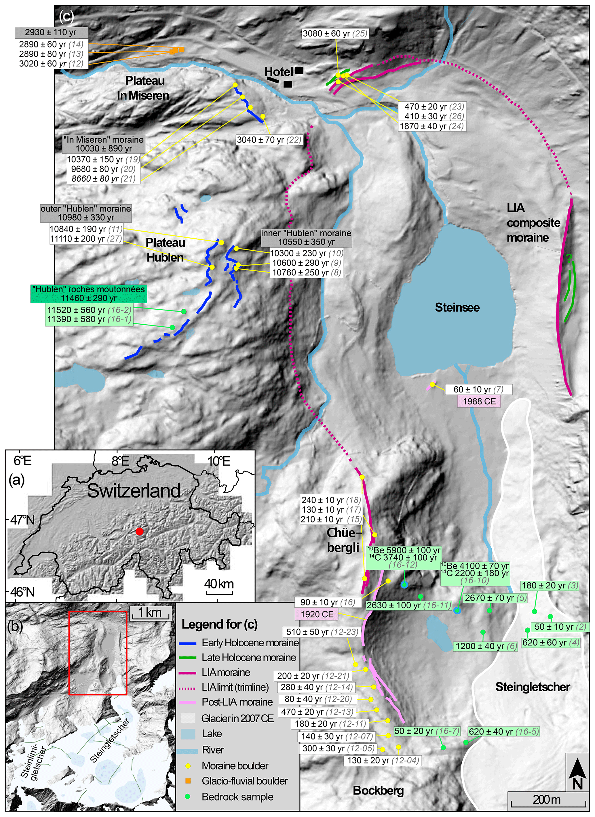
Figure 1Maps of the study site based on shaded relief ALTI3D models by ©swisstopo. (a) Switzerland and the location of Steingletscher as a red dot (central Swiss Alps, 47 ∘C). (b) Overview of the whole glacier catchment with the extents of Steingletscher and Steinlimigletscher in the year 2016. The red rectangular corresponds to panel (c). (c) Steingletscher's forefield with mapped Holocene moraines, their 10Be exposure ages and 1σ analytical uncertainties (white boxes; recalculated from Schimmelpfennig et al., 2014; one outlier in italic), and the new bedrock sample locations with their apparent 10Be and 14C exposure durations and 1σ analytical uncertainties (green boxes). Mean landform ages are shown in darker boxes with 1σ uncertainties including analytical and 10Be production rate uncertainties. Pink boxes give years of historically recorded moraine deposits.
In this study, we focus on Steingletscher, an often-visited, small mountain glacier in the central Swiss Alps (Fig. 1). Its evolution has been well-monitored since the end of the 19th century, showing that it has been constantly retreating, losing >1000 m of its length since 1985 CE as a response to the modern climate warming (GLAMOS, 2020). Its forefield has been subject to various scientific studies, including investigations of the glacier's responses to Holocene cold episodes (King, 1974; Schimmelpfennig et al., 2014). Schimmelpfennig et al. (2014) mapped and 10Be-dated the Holocene moraines in the forefield of Steingletscher (Fig. 1), providing evidence of several large glacier extents between the early Holocene and the end of the Little Ice Age (LIA, ∼14th to 19th century). This existing knowledge on the glacier's advances and its high sensitivity to warming make it an ideal target to investigate the more difficult question: how did this glacier respond to extended warm periods during the Holocene? We therefore present here new measurements of in situ cosmogenic 14C and 10Be in bedrock recently deglaciated in front of Steingletscher, generally following the approach applied at nearby Rhône Glacier (Goehring et al., 2011). We combine the new data on glacier recession with the previously published local Holocene moraine chronology, as well as with earlier published bracketing radiocarbon ages (King, 1974; Hormes et al., 2006) and historical and instrumental documentation of the recent glacier evolution. Our principal objectives are to (1) temporally constrain the Holocene intervals during which Steingletscher was at least as retracted as in modern times and (2) evaluate whether the Steingletscher and Rhône Glacier retreat histories are individual records or rather represent regional glacier responses to warming climate phases. We then put the result into the context of Holocene climate and glacier evolution in the Alps to test the significance of the HTM at regional scale.
Steingletscher is located in the eastern part of the Bernese Alps (∼47∘ N, 8∘ E) at an altitude of 2220 close to Susten Pass and is part of a larger glacier catchment that hosts another glacier, Steinlimigletscher (Fig. 1b). It had a length of 3.35 km in 2019 CE and an area of 7.6 km2 in 2013 (GLAMOS, 2019, 2020). Metagranitoids, gneisses and amphibolites constitute the geology of the glacier's surroundings. During the reference period 1991–2020 CE, the climate at the nearest weather station (Meiringen, 588 ) was characterized by an annual mean temperature of 8.7 ∘C, a monthly mean temperature range between −1.1 and 17.9 ∘C, and an annual mean precipitation of 1341 mm (https://www.meteoswiss.admin.ch, last access: 10 January 2022). During the reference period 1981–2010 CE, snow cover with a thickness of >50 cm occurred on 2.9 d (https://www.meteoswiss.admin.ch, last access: 18 July 2021; climsheet 2.1.6/5 January 2021). In the forefield of Steingletscher, the mean July temperature was 9.5 ∘C between 1991 and 2020 CE (information provided by costumer service MeteoSwiss).
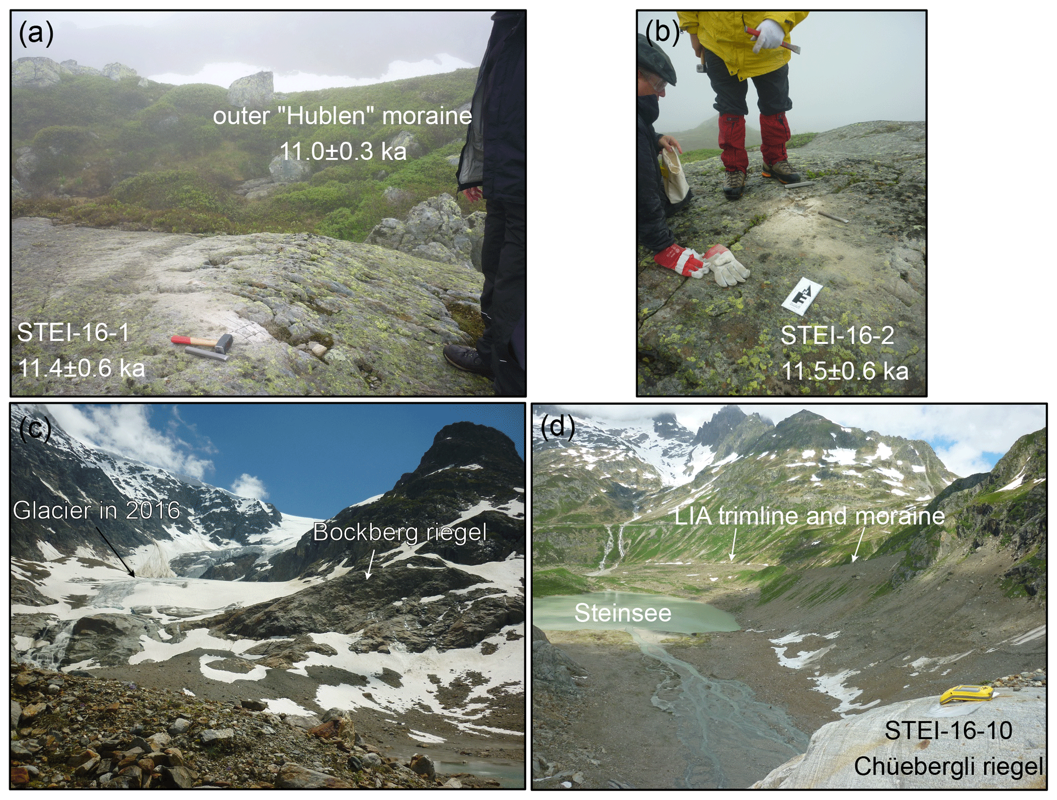
Figure 2Photographs taken during field work. (a, b) Bedrock surfaces sampled close to the summit of Hublen Plateau. (c) Bockberg riegel and the glacier terminus in the year 2016. (d) Location of sample STEI-16-10 on Chüebergli riegel with the view on the eastern side of the Steingletscher forefield, highlighting the LIA trimline and composite moraine.
Steingletscher's forefield, stretching almost linearly towards the north, features glacially smoothed hills, moraines, trimlines and the proglacial Steinsee, a lake located of the half-bowl-shaped distal part of the forefield. The catchment's outlet is located in the northwestern corner of this bowl and drains westward into Gadmen valley. On the left-lateral catchment flank, the up to 2090 m high “Plateau Hublen” and the lower “Plateau In Miseren” are characterized by glacially polished and lichen-covered bedrock knobs (roches moutonnées; Fig. 2a and b), interspersed with vegetated depressions, and small peat bogs and lakes (Fig. 1c). This landscape is overprinted by relicts of several moraine belts, i.e. the outer and the inner Hublen moraines and the In Miseren moraine, which were 10Be-dated at ∼11.0, ∼10.6 and ∼10.0 ka, from outer to inner (Schimmelpfennig et al., 2014). King (1974) obtained minimum radiocarbon ages for moraine formations from basal parts of peat bogs on Plateaus Hublen and In Miseren, which are in agreement with the 10Be Holocene moraine data (Fig. 3a). They indicate that cold conditions still persisted during the deglaciation after the Younger Dryas (YD; 12.8–11.7 ka; Rasmussen et al., 2006). However, further evidence of YD-related extents has not yet been identified. Here, we targeted two roches moutonnées located close to the highest point of Plateau Hublen, a few meters outboard of the outer Hublen moraine (Figs. 1 and 2a, b) with the objective to date the timing of initial deglaciation of this plateau.
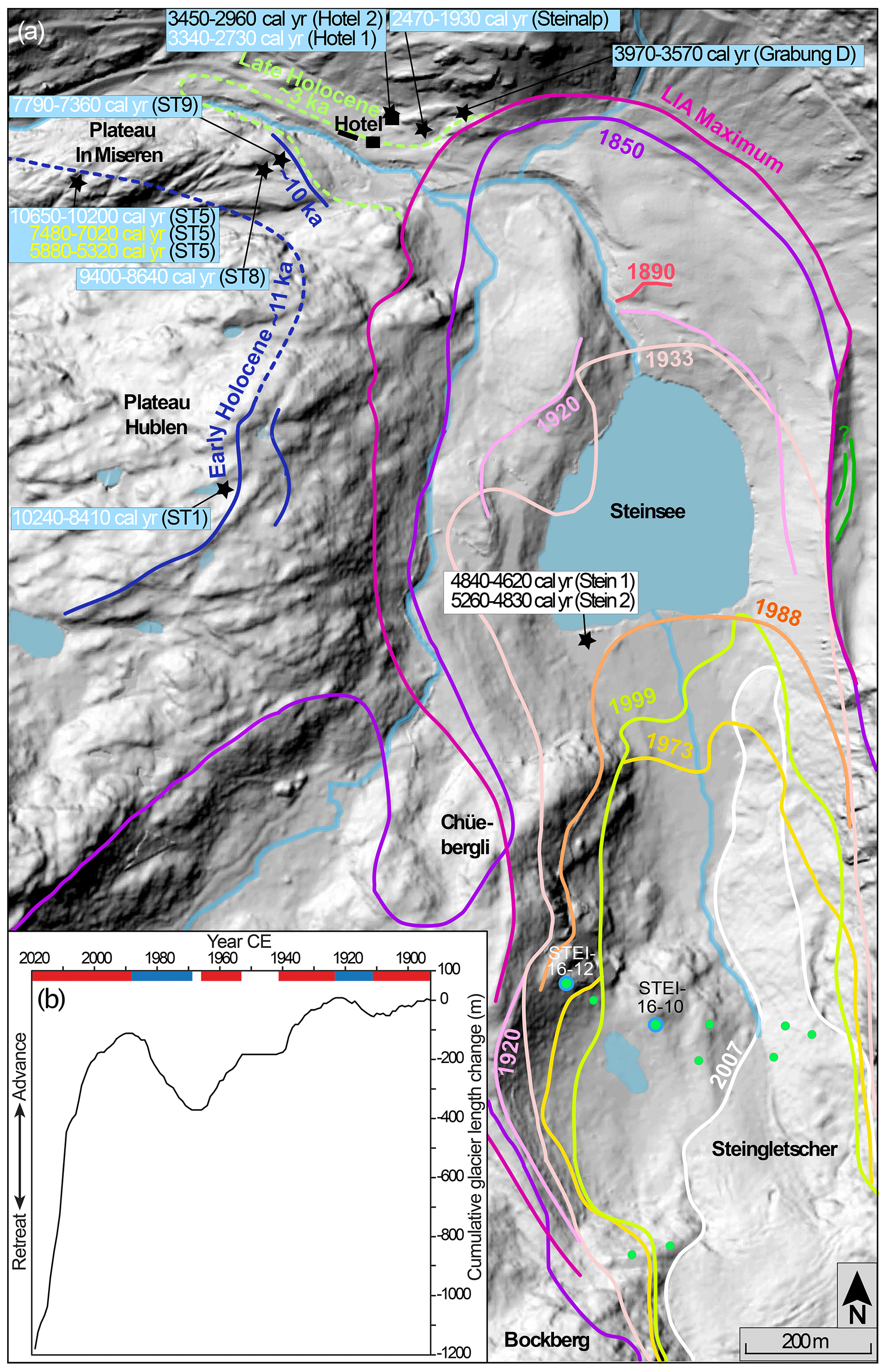
Figure 3Map of Holocene extents of Steingletscher based on 10Be moraine dating (see Fig. 1c) for the period between ∼11 ka and LIA, and on historical topographic maps and data from the Swiss Glacier Inventory (CH-INVGLAZ), adapted from Wirz (2007) and King (1974), for the period between 1850 and 1999 CE (a), on shaded relief ALTI3D model by ©swisstopo. Black stars represent locations of radiocarbon-dated organic material and corresponding calibrated ages from King (1974) (in blue boxes; black numbers are maximum ages and white numbers are minimum ages for moraine deposits or glacier retreats/advances; yellow ages correspond to certain pollen assemblages) and from Hormes et al. (2006) (in white box). Bedrock sample locations on Chüebergli and Bockberg riegels are shown as green dots, and samples STEI-16-10 and -12 are highlighted with blue rims. (b) Length measurements of Steingletscher since 1893 (from GLAMOS, 2020). Red and blue bars correspond to trends of glacier retreat and advance, respectively; intervals of glacier stagnation are in white.
The absence of moraines after ∼10 ka and throughout the mid-Holocene indicates a warmer climate at that time (Schimmelpfennig et al., 2014). This is supported by radiocarbon ages of ∼9 ka cal BP and from the mid-Holocene obtained from peat bogs on Plateau In Miseren (King, 1974; Table 2 in Schimmelpfennig et al., 2014; Fig. 3a). In addition, evidence of a substantially retracted mid-Holocene extent of Steingletscher comes from two wood fragments melted out from the glacier front between 1995 and 2000 CE and radiocarbon-dated at 5.3–4.8 and 4.8–4.6 ka cal BP (Hormes et al., 2006; Fig. 3a). In the same study, two organic silt samples from the forefield of the neighboring Steinlimigletscher, also collected between 1995 and 2000 CE, were radiocarbon-dated at 5.9–5.3 and 2.3–1.8 ka cal BP. Further information on the amplitude and duration of glacier recession during the early and mid-Holocene is missing, as geomorphic markers of glacier extents during that time were destroyed by the glacier re-advances during late Holocene cooling.
Evidence of late Holocene moraine formation comes from glacial boulders in the vicinity of the catchment outlet dated at ∼2.9 ka (Schimmelpfennig et al., 2014). This maximum glacier extent during the late Holocene is corroborated by radiocarbon dates of organic material from soil and peat on the right-lateral side of the catchment outlet, which provide bracketing ages for the glacier advance and retreat around 3 ka ago (King, 1974; Table 2 in Schimmelpfennig et al., 2014; Fig. 3a). One large moraine boulder located on a ridge inboard of the ∼3 ka moraine was 10Be-dated at ∼1.9 ka and might represent a glacier extent at that time (Schimmelpfennig et al., 2014).

Figure 4Aerial photograph of Steingletscher terminus position in 1982 CE with indications of the timing of earlier glacier extents, from http://www.swisseduc.ch (last access: 10 January 2022). The location of the Chüebergli sample profile is indicated by the green box. Ice thickness in 1982 CE is estimated at ∼50 to ∼20 m above the analyzed samples.
The most evident geomorphic markers of glacier expansion in Steingletscher's forefield are those from the Little Ice Age, including a sharp composite moraine on the eastern side of the forefield (Fig. 2d), multiple moraine ridges, and a clearly visible trimline (Figs. 2d and 4). Boulders from the preserved moraines yield 10Be ages between ∼570 and 140 years, consistent with the period of the LIA (Schimmelpfennig et al., 2014).
Historical and instrumental records provide constraints on glacial extents during the general retreat between 1850 CE and the beginning of the 21st century, which are here mainly based on previous compilations by King (1974) and Wirz (2007) and on glacier length measurements (GLAMOS, 2020). Figure 3a shows the glacier outlines in the years 1850, 1920, 1933, 1973, 1988, 1999 and 2007. The length measurements of Steingletscher between the years 1893 and 2019 (Fig. 3b) indicate that the glacier had never retreated as much as in 2007 during that time. The most pronounced retreat of the 20th century occurred between 1960 and 1970, leading very briefly to a minimum extent that was comparable to that of the very beginning of the 21st century, but still slightly bigger than that in 2007 (Fig. 3b). During the subsequent advance of the 1970–1980s the glacier reached as far as into Steinsee. Since 1988, the glacier has been rapidly and continuously retreating and has lost >1000 m of its length in response to the modern global warming. Steingletscher is thus currently not in equilibrium with climate but lags behind the accelerating warming by up to several decades.
To investigate how Steingletscher responded to naturally driven Holocene warmth, specifically how long it was similar in size to its modern configuration during the Holocene, we targeted two bedrock riegels for in situ 14C–10Be exposure–burial dating. One riegel is located east of Chüebergli (“Chüebergli riegel” hereafter) and is ∼400 m long. The other riegel is located north of Bockberg (“Bockberg riegel” hereafter) and is ∼200 m long. Both riegels are characterized by glacially polished, recently deglaciated roches moutonnées (Fig. 2c and d) that form steep cliffs towards the north. Chüebergli riegel was completely covered under at least ∼140 m of ice during the LIA maximum, inferred from the altitude of the LIA composite moraine and trimline on the eastern catchment flank, and continued to be buried throughout most of the 20th century. Eight samples were collected on a transect on Chüebergli riegel from the highest and outmost bedrock surface down to the lowest bedrock surface in the glacial trough, following the sampling approach in Goehring et al. (2011). Note that the three lowest sample surfaces were still covered by ice in 2007 (Fig. 1c) but were ice-free by the sampling year 2010. From Bockberg riegel, two samples were analyzed (Fig. 1c).
After the glacier retreat in the 1960s, the outmost parts of the two riegels were temporarily ice-free, but ice-covered again in the 1970s–1980s by ∼20 m of ice (Figs. 3a and 4). Chüebergli riegel might have been completely ice-free briefly around 1970. Both riegels were deglaciated in the early 21st century, and Steingletscher has continued to retreat since.
3.1 Fieldwork
The 14 bedrock samples were collected during field campaigns in 2010 and 2016, targeting glacially polished and striated surfaces that were free of sediment cover. To minimize the risk of significant snow and sediment cover in the past, slightly sloping surfaces were preferred (Fig. 2d). Rock surface pieces with average thicknesses of ∼2 to ∼4 cm (Table 1) were sampled using either hammer and chisel alone or in combination with a cordless angle grinder and a diamond blade. Primarily the quartz-rich parts of the gneissic lithologies were targeted. Latitude, longitude and elevation at the sample locations were recorded with a Trimble GeoTX GPS; the data reduction was conducted using the WGS coordinate system relative to EGM896 Geoid (Table 1). Correction factors for the shielding by the surrounding topography and the strike and dip of the sampled surfaces were determined from measurements using a handheld inclinometer. These correction factors range from 0.87 to 1.0 (Table 1).
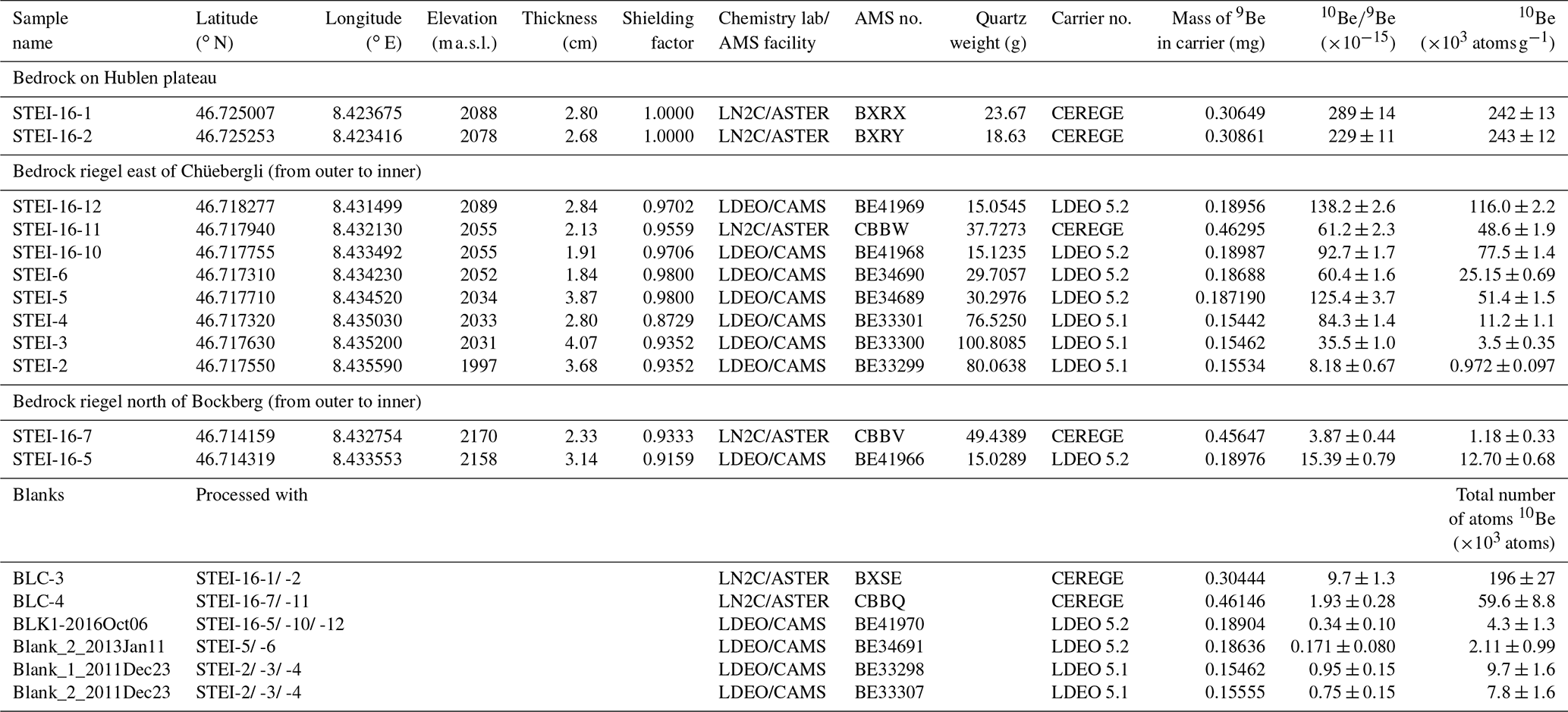
Table 1Sample field information and analytical 10Be data. Carrier solution “CEREGE” used at LN2C has a 9Be concentration of 3025 µg g−1; ratios measured at ASTER (Arnold et al., 2010) were normalized to in-house standard STD-11 with the ratio of (Braucher et al., 2015). LDEO carrier solutions “5.1” and “5.2” have 9Be concentrations of 1024 and 1031.78 µg g−1, respectively; ratios measured at CAMS were normalized to standard 07KNSTD with the ratio (Nishiizumi et al., 2007). A 10Be half-life of years was used (Chmeleff et al., 2010; Korschinek et al., 2010). Samples were corrected for chemistry blanks by subtracting the number of atoms 10Be in the corresponding blank from that of the sample.
3.2 Analytical methods
We separated and decontaminated quartz from 14 samples and extracted 10Be from the clean quartz after spiking it with a pure 9Be carrier (Table 1). Chemical processing was carried out at the Lamont-Doherty Earth Observatory (LDEO) Cosmogenic Nuclide Laboratory (New York, USA) according to the standard procedures described in Schaefer et al. (2009) and at the Laboratoire National des Nucléides Cosmogéniques (LN2C) at the Centre Européen de recherche et d'Enseignement des Géosciences de l'Environnement (CEREGE, Aix en Provence, France) following routine methods described for example in Protin et al. (2019). ratios were measured at the Lawrence Livermore National Laboratory – Center for Accelerator Mass Spectrometry (LLNL-CAMS) and at Accélérateur pour les Sciences de la Terre, Environnement, Risques (ASTER) at CEREGE. All data related to the 10Be analyses are presented in Table 1.
In situ 14C was extracted from the quartz of the two bedrock samples from Chüebergli riegel with the highest 10Be concentrations (STEI-16-10 and -12). These extractions were performed at LDEO following the procedure described in Goehring et al. (2014) and Lamp et al. (2019), with two updates: the purified CO2 sample and blank gas were diluted with only small amounts of 14C-free gas corresponding to ∼20 µg of C (Table 2); the sample and dilution gas mixtures were not converted into graphite, but sealed into pyrex break seals for ratio measurements at the AixMICADAS facility at CEREGE using the ion source dedicated for gaseous samples (Bard et al., 2015; Tuna et al., 2018), thus avoiding the graphitization step. 14C concentrations were calculated following the method of Hippe and Lifton (2014) (Table 2).
Table 2Analytical in situ 14C data. “Mass C (µg) sample” and “Mass C (µg) sample + diluted” are the masses of carbon released during extraction and after addition of 14C-free dilution gas, respectively. Oxalic acid OX-II is used as AMS standard, and all measurements are corrected for the AMS machine background blank with a ratio of 0.0023. The percent of modern carbon value (pmC) includes the d13C correction, which is undone following the calculations of Hippe and Lifton (2014). Samples were corrected for the procedural blank by subtracting the number of atoms 14C in the blank from that of the samples. The apparent 14C ages do not account for subglacial erosion effects and are therefore minimum ages, referenced to the sampling year 2016. See text for parameters used for the age calculations.
3.3 Principles of the exposure–burial dating approach
Three types of glacial surfaces with different exposure histories are investigated in this study.
- i.
Moraine boulders. They can in most cases be assumed to have a simple exposure history; i.e., they were free from cosmogenic nuclides at the moment of their stabilization after the glacier had retreated from its advance and have since been continuously exposed. In this case, the analysis of 10Be alone usually provides the exposure age of the surface. Based on the consistency of the 10Be moraine boulder ages of Schimmelpfennig et al. (2014), they seem to fulfill this condition.
- ii.
Bedrock surfaces that remained continuously ice-free during the Holocene. They are located outboard of the maximum Holocene glacier extent. We assume that they were covered long enough and subglacially eroded deep enough during the ∼100 ka lasting last glacial period that ended with the YD that these surfaces were free from cosmogenic nuclides at the moment of their last deglaciation. Subsequently, they experienced a simple exposure history, if cover by sediment, soil or vegetation is negligible. The two dated bedrock samples from Hublen (STEI-16-1 and -2), located outboard of the outer Hublen moraine, are assumed to fulfill these conditions.
- iii.
Bedrock surfaces that were alternately ice-free and ice-covered during the Holocene. They are located inboard of all Holocene moraines. Like the bedrock type ii, their cosmogenic nuclide inventory is assumed to have been set to zero during the last glacial period. If during the Holocene phases of no glacier cover were followed by glacier cover during 102–103-year periods and with moderate subglacial erosion, cosmogenic nuclide concentrations accumulated from several exposure periods but were reduced through the glacial erosion during ice cover. Consequently, the analysis of 10Be alone in this type of sample provides a minimum duration of the cumulative exposure period. The 10 samples from Chüebergli and Bockberg riegels correspond to this type of bedrock.
In the case of the bedrock type iii, the combined analysis of 10Be and 14C allows for solving for the unknown exposure duration and erosion depth, if the moment of initial deglaciation can be constrained (see Sect. 3.5). This is because 14C (half-life 5.7 kyr) decays much faster than 10Be (half-life 1.39 Myr, Chmeleff et al., 2010; Korschinek et al., 2010), and therefore their concentrations evolve differently as a function of exposure and burial: during exposure both nuclides accumulate at a nearly constant rate with the concentration ratio close to ∼3; during burial under ice, production stops and only the decay of the 14C concentration is notable on these relatively short timescales, leading to lower concentration ratios (Fig. 5; Hippe, 2017). In addition, subglacial erosion of the initially exposed surface removes the superficial bedrock layers, thereby advecting less 14C and 10Be concentrated rock from depth to the surface (Fig. 5). If this subglacial erosion is negligible or largely dominated by abrasion, the concentration ratio is less than 3 in the collected samples (Fig. 5), while higher ratios indicate surface quarrying by the glacier (Rand and Goehring, 2019). The latter is because production at depth of 14C is higher relative to that of 10Be due to a higher 14C contribution from muons, which penetrate deeper under the subsurface than neutrons (Hippe, 2017). Thus, in the case of moderate erosion rates dominated by abrasion, the apparent (i.e., non-burial- and erosion-corrected) 10Be and 14C ages provide both minimum exposure durations, with apparent 14C ages being younger than their 10Be counter parts, and the concentration ratio less than ∼3.
Figure 5General concept of the in situ 14C–10Be exposure–burial approach. Left panels show a hypothetical scenario of alternating large and retracted glacier extents, covering and uncovering a fictive sample location (red spot). Middle panels depict the position of the sample material (red rectangle) with regard to the bedrock surface. Right panels of stages (2) and (3) illustrate the trajectories of the in situ 14C and 10Be concentrations in the sample during its exposure and advection (exhumation) towards the surface (Lagrangian perspective; see Sect. 3.5). Stage (1): subsequent to continuous ice cover and deep subglacial erosion during the last glaciation, the bedrock is free from cosmogenic nuclides. Deposition of the early Holocene (EH) moraines and subsequent glacier retreat constrains the beginning of the Holocene glacier retreat, i.e., 10 ka in this example. Stage (2): the sample location is exposed for an unknown duration texp, with the sample material remaining at the same depth (no surface erosion), where 14C and 10Be accumulate constantly. Stage (3): the sample location is buried by ice, which abrades the bedrock surface, thus progressively exhuming the sample material. No production of 14C and 10Be due to shielding by ice cover. Radioactive decay leads to steady loss of 14C (short half-life of 5.7 kyr) but does not affect the 10Be concentration due to the long half-life of this nuclide of 1.4 Myr. The burial duration tb is equal to the timing of initial EH glacier retreat minus texp. The dashed line represents the initially exposed surface elevation. Stage (4): exposed since the recent glacier retreat, the sample material is now at the surface where it is collected. E represents the unknown erosion depth, i.e., the thickness of rock layer that was removed by abrasion during stage (3). The lowest right panel shows a two-isotope plot with the thick black line representing continuous exposure ( ratio = ∼3) and the grey area burial and subglacial abrasion ( ratio <3). The ratio and 10Be concentration of the fictive sample is plotted as a red dot.
We make the assumption that during the periods of burial, the ice cover was always thick enough at our sample locations to hinder significant 14C accumulation via muogenic production. Shielding by >70 m of ice is required to reduce 14C production to 1 % of its surface production, and under a thin ice cover of ∼13 m 14C is produced at 10 % compared to an ice-free surface, while 10Be is produced at only 1 % (Hippe, 2017). The photograph in Fig. 4 allowed us to estimate that during the glacier extent in 1982, ice cover was on the order of ∼20 to 50 m above the sample locations, suggesting that 14C production in the subglacial rock surfaces during episodes of ice cover should be small enough to not significantly affect the interpretation of our data.
This exposure–burial bedrock dating approach thus allows us to determine the cumulative duration that the glacier retreated beyond the sample locations during the Holocene. As reference for this minimum amplitude of retreat, we refer to the extent in modern times when the glacier uncovered the sample locations for the last time, i.e., ∼1999 CE for sample STEI-16-12 and ∼2007 CE for sample STEI-16-10 (Fig. 3a). As the time elapsed between these two years is insignificant compared to the centennial to millennial timescales investigated here, we simplify and refer to 2000 CE for both sample locations.
3.4 Calculations of simple exposure ages
The 10Be moraine and apparent bedrock ages discussed below were calculated with CREp (http://crep.crpg.cnrs-nancy.fr/#/, last access: 11 January 2022; Martin et al., 2017), choosing the local “Alpine” 10Be spallation production rate (Claude et al., 2014) (4.11±0.10 as calculated in CREp via the link to the ICE-D calibration database), the ERA40 atmosphere model (Uppala et al., 2005) and Lal–Stone time-corrected scaling (Lal, 1991; Stone, 2000; Balco et al., 2008) with atmospheric 10Be-based VDM (Muscheler et al., 2005; Valet et al., 2005). The apparent 14C bedrock ages were calculated accounting for spallogenic and muogenic production and radioactive decay, using the global 14C spallation production rate of 12.22±0.89 , the muon parameters from Balco (2017) and the half-life of 5730 years. The same atmosphere model and scaling methods as for 10Be were applied. A density of 2.7 g cm−3 is assumed for all samples.
As most of the recent studies in the Alps used the former CRONUS-Earth calculator by Balco et al. (2008) to calculate cosmogenic nuclide ages, we also show the 10Be moraine and apparent 10Be and 14C exposure durations of bedrock calculated with version 3 of this tool, choosing the same parameters as above regarding the 10Be production rate (calculated as 4.04±0.38 in the former CRONUS-Earth calculator using the calibration data from the ICE-D calibration database), atmosphere model and scaling scheme. Note that the calculator applies default parameters for the geomagnetic field model and the 14C production rate.
All 10Be and 14C exposure ages and durations are shown in Tables 2 and 3. 10Be exposure ages and durations calculated with both calculators differ by 1 %–2 % for early Holocene ages, and by at most 8 % for younger ages and exposure durations. 14C exposure durations differ by 3 %–5 %. Higher differences in the results are due to high late Holocene inter- and intra-variability in the geomagnetic field records used in both calculators.
Table 310Be moraine ages and apparent 10Be bedrock ages at Steingletscher, with their full 1σ uncertainties. The uncertainties in parentheses are the analytical 1σ uncertainties in the case of individual ages and standard deviations in the case of mean ages. Moraine ages are recalculated from Schimmelpfennig et al. (2014), using the same methods as for the bedrock samples (see Sect. 3.4). One outlier is in italics. The apparent 10Be exposure ages do not account for subglacial erosion effects and are therefore minimum ages (with reference to the year of sampling). All moraine ages and bedrock ages from Hublen are referenced to 1950 CE.
Unless otherwise stated, in situ cosmogenic ages corresponding to glacial surface types i and ii are reported in the text, tables and figures with the unit ka (“thousand years ago”) with reference to 1950 CE (before BP), i.e., 60–66 years were deduced from their exposure ages. Exposure and burial durations of type iii bedrock are given with the unit kyr and refer to their year of sampling (2010 or 2016 CE).
3.5 Modeling of complex bedrock exposure history and erosion depth
Regarding the complex exposure history of bedrock type iii, three variables are unknown: the cumulative exposure duration texp, the cumulative burial duration tb and the erosion depth E, while the two-nuclide system allows for two of these unknowns to be solved (Goehring et al., 2011). In our study, the age of the youngest early Holocene moraine (In Miseren moraine, ∼10 ka), provides the timing of initial deglaciation of Steingletscher's forefield, and therefore the cumulative burial duration can be constrained by (Fig. 5; Goehring et al., 2011). In the pioneer Rhône Glacier study by Goehring et al. (2011) the remaining two unknowns, texp and E, were determined for each sample through the classical Eulerian computation, i.e., using the two equations for 10Be and 14C production and loss at the rock surface. In a follow-up study, Goehring et al. (2013) proposed in addition an isochron Bayesian approach that allows several samples to be considered simultaneously with the purpose of reducing the uncertainties for the whole data set.
Here, we use the Lagrangian instead of the Eulerian calculation method (Knudsen et al., 2019), combined with a Monte Carlo–Markov chain (MCMC) inversion to constrain the values of texp and E. We define a forward model to predict 10Be and 14C concentrations as a function of texp and E in each of the two 10Be- and 14C-analyzed rock samples (STEI-16-10 and -12) during their advection toward the surface, as schematically illustrated in Fig. 5. For this, we apply the same production parameters and scaling method as for the simple exposure age calculations. We assume that the 10Be and 14C concentrations were set to zero due to deep and sustained glacial erosion during the previous glacial phase (Fig. 5). The onset of the exposure history is set at 10 ka, as constrained by In Miseren moraine. The subsequent history is divided into two steps. First, the surface is exposed for a duration texp, leading to steady accumulation of 10Be and 14C. Second, the surface is covered by ice until the present, leading to zero nuclide production, but bedrock erosion of a thickness E. The corresponding hypothetical 10Be and 14C concentration–time trajectories are shown in Fig. 5. We then use a standard MCMC approach to sample the parameter plane defined by texp and E with the Metropolis–Hastings algorithm and obtain the posterior distributions of these parameters for both samples. For each sample, we run six MCMC chains of length 105, including a 103 burn-in phase. For each parameter we report the average and standard deviation of the chain. The average erosion rate ε is subsequently determined by .
The advantage of using the Lagrangian instead of the Eulerian approach is that it is more flexible when calculating the changing nuclide concentrations in a bedrock sample during its advection to the surface (Knudsen et al., 2019). In our specific case it conveniently allows the depth-dependent production and decay of 14C to be considered as a function of time, instead of summing up nuclide production and loss in a virtual surface sample. However, we stress that in our application, no significant differences result from the two approaches. Figure 7l indeed depicts the concentration–time trajectories at the surface, i.e., using the Eulerian approach, both for the above-described single exposure–burial scenario and a more complex scenario with several exposure–burial alternations.
3.6 Recalibration of previously published radiocarbon dates
The radiocarbon ages previously published in King (1974) and Hormes et al. (2006) and discussed in this study were calibrated with the online program OxCal 4.4 (Bronk Ramsey, 2009), using its standard options and the IntCal20 calibration curve (Reimer et al., 2020), and are reported relative to the year 1950 CE. This changes the 2σ age intervals by at most 6 % compared to the calibration with the earlier OxCal 3.9 version presented in Hormes et al. (2006). The radiocarbon ages published in King (1974) were uncalibrated and can therefore not be compared to the ages calibrated in our study. Note that with regard to the original studies, the general interpretations of all radiocarbon ages discussed here remain unaffected from the (re)calibration.
Tables 2 and 3 and Figs. 1c and 6a show the exposure ages and apparent exposure durations directly calculated from the measured 10Be and 14C concentrations. Also listed in Table 3 are all 10Be moraine boulder ages and moraine mean ages previously published in Schimmelpfennig et al. (2014) and recalculated with the methods presented in Sect. 3.4. In the tables, ages are shown with their full uncertainties (i.e., including analytical and production rate uncertainties) and analytical uncertainties only. In the text and in the figures, the individual ages are presented with their analytical uncertainties only, while moraine mean ages are presented in the text and in the figures with their full uncertainties, i.e., standard deviation and production rate error combined through simple error propagation (square root of the sum of their values in quadrature).
Figure 6Exposure durations of bedrock samples inferred from measured in situ 10Be and 14C concentrations. (a) Apparent exposure durations calculated from 10Be concentrations of eight samples and 14C concentrations of two samples as a function of position in the glacial trough profile. The subglacial erosion effect during ice burial is not accounted for; calculations therefore yield minimum exposure durations. (b) Exposure durations and erosion depths modeled from combined in situ 10Be and 14C concentrations of samples STEI-16-10 and -12 (orange and green signatures). Solid grey curves represent possible exposure duration and erosion–depth combinations for samples with 10Be concentration only. Yellow lines indicate selected theoretical bedrock erosion rates.
The two 10Be bedrock samples from Plateau Hublen yield indistinguishable ages of 11.39±0.58 ka (STEI-16-1) and 11.52±0.56 ka (STEI-16-2) with an arithmetic mean age of 11.5±0.3 ka.
The two oldest apparent 10Be bedrock exposure durations from the Chüebergli riegel profile are 5.90±0.10 kyr (STEI-16-12) and 4.10±0.07 kyr (STEI-16-10). The other samples on this profile range between 2.67±0.07 kyr (STEI-5) and 0.05±0.01 kyr (STEI-2). All eight apparent 10Be ages from the profile present a general trend from high values at the outer margin towards low values at the inner, lowest sample locations (Fig. 6a). This trend is consistent with the higher ice flow velocity in the center of a glacial trough that leads to deeper subglacial bedrock erosion during periods of ice cover, thus reducing the 10Be surface concentrations at a higher rate (Goehring et al., 2011).
Only the two samples with the oldest apparent 10Be exposure durations (STEI-16-12 and STEI-16-10) were chosen for 14C analyses to ensure 14C measurements precise enough for a meaningful interpretation. The apparent 14C exposure durations of the two analyzed samples are 3.74±0.10 and 2.20±0.05 kyr, respectively; i.e., both are apparently younger than their 10Be counterparts. This trend and the low concentration ratios of 1.67±0.05 and 1.62±0.04, respectively, are consistent with temporary burial of the surfaces and indicate that subglacial erosion was moderate and dominated by abrasion (see Sect. 3.3; Table 2).
The two apparent 10Be bedrock exposure durations from the Bockberg riegel are 0.05±0.02 kyr (STEI-16-7) and 0.62±0.03 kyr (STEI-16-5). We decided to not use them for 14C analyses due to the low cosmogenic nuclide inventory. These samples are therefore only briefly discussed in the following text.
We highlight the exceptionally young apparent ages of samples STEI-2 and STEI-16-7, prepared/measured at LDEO/CAMS and LN2C/ASTER, respectively (Table 1), showing that at these facilities we are able to detect 10Be signals that correspond to ages as young as ∼50 years with 20 %–40 % analytical uncertainty.
Modeling of the 10Be and 14C data yields cumulative exposure durations texp for STEI-16-12 and STEI-16-10 of 8.0±0.3 and 6.8±0.3 kyr (1σ analytical uncertainties), burial durations tb of 2.1±0.1 and 3.2±0.1 kyr, and subglacial erosion depths E of 21±3 cm and 36±3 cm. This corresponds to erosion rates ε of 0.10 ± 0.02 mm yr−1 and 0.11 ± 0.01 mm yr−1, respectively. Following the assumption that samples on a transect parallel to the ice flow experienced the same exposure history on millennial timescales (Goehring et al., 2011), an average ice-free duration and standard deviation of 7.4±0.8 kyr can be deduced from the results of STEI-16-12 and STEI-16-10. Given that STEI-16-12 lies ∼160 m further outboard and 34 m higher in elevation than STEI-16-10, the longer exposure duration derived for STEI-16-12 could also either be due to shorter ice cover or be an artifact of a thinner ice cover above this sample, the latter potentially leading to small muogenic 14C production in the subglacial surface of the sample (see Sect. 3.3). Distinct exposure histories of the two sample locations are explored in Sect. 5.1.
Figure 6b shows the texp and E distributions that can explain the observed concentration of one nuclide alone, 10Be or 14C, resulting from the forward model (see Sect. 3.5) and represented by plain and dashed curves, respectively, for each sample (colored curves). The intersection of the two curves coincides with the average texp and E values, determined with the MCMC inversion, thus providing a visual check of the optimal model solution. Following this strategy, we added the same type of curves obtained from the 10Be concentrations alone of four other samples from Chüebergli riegel (grey curves; not shown are the results from the two innermost samples due to their low 10Be concentrations). This approach allows evaluation of the range of possible erosion depths and rates, illustrated by the yellow lines, even without combination with 14C analyses. Assuming that these four samples experienced a similar exposure–burial history to samples STEI-16-12 and STEI-16-10, their 10Be concentrations indicate subglacial erosion rates of >0.2 mm yr−1 (Fig. 6b). This erosion rate estimate and the values inferred from the combined 10Be and 14C data (∼0.10–0.11 mm yr−1) agree with those from Rhône Glacier (∼0.02–0.33 mm yr−1) and the steep Trift riegel (0–>2 mm yr−1) obtained with the same analytical method (Goehring et al., 2011; Steinemann et al., 2021).
5.1 Holocene timing and duration of Steingletscher retreat
Given the similarity in ages of the Hublen bedrock (highest and stratigraphically outmost position; 11.5±0.3 ka) and the outer Hublen moraine (11.0±0.3 ka), we infer that these bedrock surfaces experienced a simple exposure history and that their age represents the timing of the first general deglaciation of the summit of Plateau Hublen at ∼11.5 ka, during the transition from the YD to the Holocene. This supports our assumption that the Hublen bedrock was free from significant 10Be inheritance from earlier interglacials (see Sect. 3.3), thus providing evidence that this is the case for any bedrock surface further inboard in Steingletscher's forefield.
This date of deglaciation of the plateau summit also implies that the glacier had a greater extent prior to ∼11.5 ka. However, chronological constraints on positions of Steingletscher prior to or during the YD do not currently exist.
Subsequent to the ∼11.5 ka deglaciation of the Hublen Plateau summit, Steingletscher experienced a slow oscillatory retreat for about 1.5 kyr, similar to other glaciers in the Alps (Protin et al., 2021), and deposited the three preserved early Holocene moraines on Plateaus Hublen and In Miseren. Steingletscher's forefield was thus most likely completely covered by ice until the deposition of the In Miseren moraine (10.0±0.9 ka). Chüebergli riegel was covered by at least 140 m of ice until then. Subsequently, the glacier retreated considerably, most probably for the first time in the Holocene. Although the amplitude of Steingletscher's recession at that time is unknown, we assume that Chüebergli and Bockberg riegels already became ice-free at ∼10 ka. This is supported by radiocarbon-dated subfossil wood relicts that melted out of several glaciers across the Swiss Alps between 1990 and 2006 CE, indicating that the tree line had been well above the wood sample localities and that these glaciers were equally small or smaller between ∼10 and ∼8.2 cal BP than between 1990 and 2006 CE (Hormes et al., 2001, 2006; Joerin et al., 2006, 2008; Nicolussi and Schluechter, 2012).
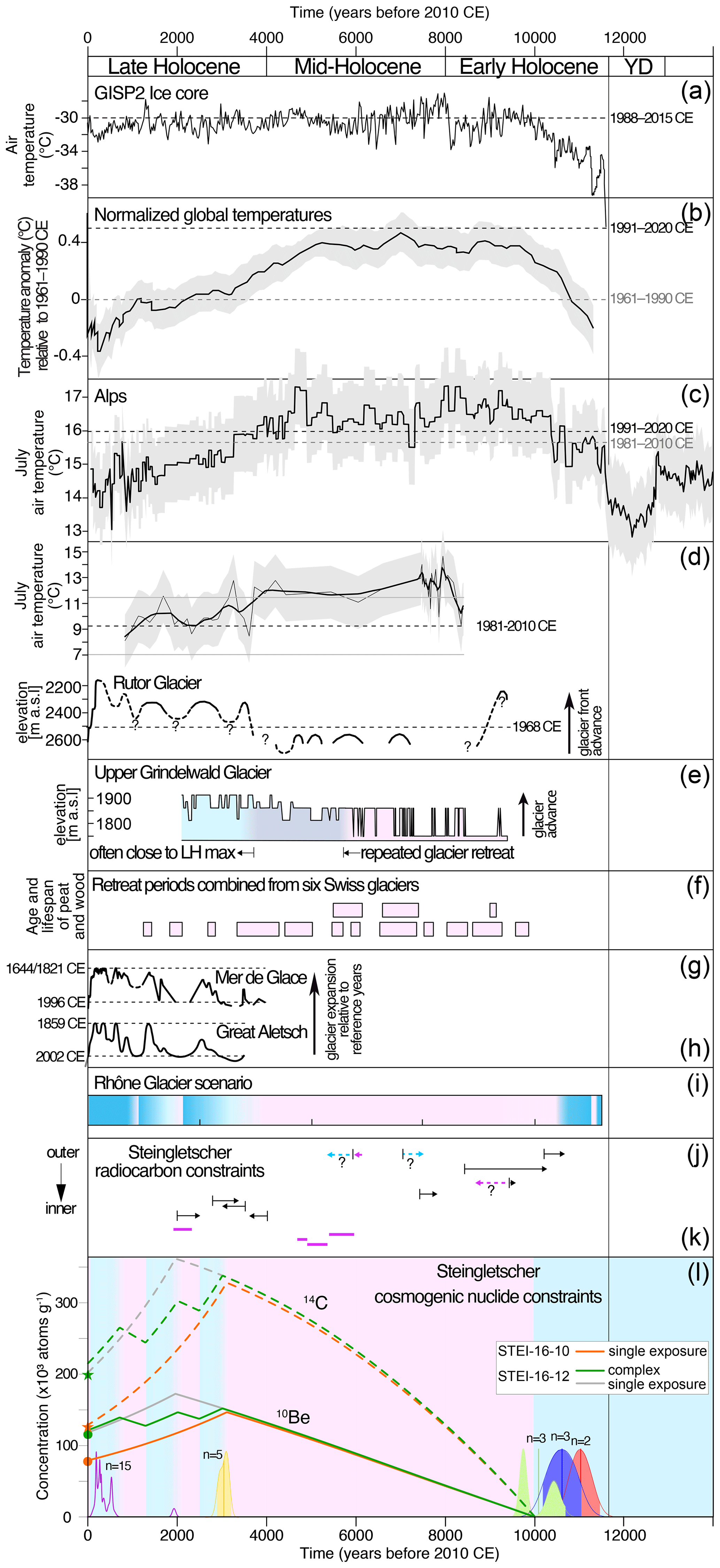
Figure 7Holocene advance and retreat history of Steingletscher (l) in comparison with independent records. (a) Greenland summit temperatures (Kobashi et al., 2017). (b) Global temperature anomalies relative to 1961–1990 CE (Marcott et al., 2013). The black dashed line is the global annual mean temperature anomaly in 1991–2020 CE (https://data.giss.nasa.gov/gistemp/, last access: 10 January 2022). (c) Chironomid-based stacked summer temperature at 1000 (Heiri et al., 2015). The dashed lines are the modern July temperatures at the weather stations closest to Hinterburgsee and Stazersee, i.e. Meiringen (588 ) and Samedan (1708 ) (https://www.meteoswiss.admin.ch, last access: 10 January 2022), extrapolated to 1000 , using a lapse rate of 6 as in Heiri et al. (2015). (d) Pollen-inferred summer temperatures from the Rutor Glacier forefield (Italian Alps), modern July temperature and uncertainty as horizontal lines. Fluctuations of Rutor glacier in comparison to 1968 CE (Badino et al., 2018). (e) Speleothem-based elevation changes of Upper Grindelwald Glacier (central Swiss Alps) (Luetscher et al., 2011). (f) Recession periods of six Swiss glaciers based on radiocarbon-dated subfossil wood and peat (Joerin et al., 2006). (g, h) Glacier fluctuations of Great Aletsch (central Swiss Alps; length changes) and Mer de Glace (northern French Alps; altitude changes) based on radiocarbon-dating and dendrochronology (Holzhauser et al., 2005; Le Roy et al., 2015, respectively). The grey extension added to the curve of Great Aletsch is the loss in length until 2020 CE (http://www.glamos.ch/en/factsheet#/B36-26, last access: 10 January 2022). (i) Holocene advance and retreat scenario of Rhône Glacier, central Swiss Alps (Goehring et al., 2011). (j) Bracketing radiocarbon ages from Steingletscher forefield (King, 1974) with arrow lengths corresponding to the 2σ age intervals. Plain arrows stand for moraine deposits or glacier advances. Dashed arrows correspond to pollen-inferred climate cooling (blue) or warming (pink) trends. (k) Radiocarbon dates of organic samples melted out from Steingletscher and Steinlimigletscher, with line lengths corresponding to the 2σ age intervals (Hormes et al., 2006). (l) Steingletscher advance and retreat scenario (this study). Summed probability curves are mean 10Be moraine ages (Schimmelpfennig et al., 2014). The modeled in situ 14C and 10Be concentrations are trajectories at the bedrock surface (Eulerian perspective). Blue bands are periods dominated by glacier positions larger than in ∼2000 CE; pink bands are periods with dominantly smaller glacier extents.
Apart from two wood fragments collected in Steingletscher's forefield and radiocarbon-dated at 5.3–4.8 and 4.8–4.6 cal ka testifying to a glacier recession upstream of its ∼2000 CE extent, no further direct constraints exist for the timing and amplitudes of Steingletscher's fluctuations during the mid-Holocene (Hormes et al., 2006; Fig. 7k). Evidence of recession of the neighboring Steinlimigletscher at 5.9–5.3 cal ka suggests that Steingletscher was in a retreated position, too, at that time (Hormes et al., 2006). During the late Holocene, the glacier readvanced considerably at ∼3 ka ago and covered Chüebergli riegel again with ∼140 m of ice or more. This happened again from at the latest 0.6 ka onward during the period of the LIA until the general retreat trend from 1850 CE on, which eventually uncovered Chüebergli riegel completely around 2000 CE. Between ∼3 ka and the LIA, the exact timing of further Steingletscher fluctuations is unknown. The bracketing radiocarbon age of a wood fragment of ∼2.5–1.9 cal ka at the base of a ∼1.10 m deep peat profile on fluvioglacial deposits near the LIA glacier limit points to glacier retreat (King, 1974). Significant glacier recession to modern extents at that time has also been documented at other Alpine glaciers, in particular in the detailed late Holocene records at Great Aletsch (Holzhauser et al., 2005) and Mer de Glace (Le Roy et al., 2015) (Fig. 7g and h). At Steinlimigletscher, one organic silt sample radiocarbon-dated at ∼2.3–1.8 cal ka, attesting to glacier retreat beyond the ∼2000 CE extent, supports a local impact of this probably regional-scale warming event (Hormes et al., 2006; Fig. 7k). A subsequent readvance of Steingletscher is tentatively suggested by one 10Be boulder age of ∼1.9 ka (Schimmelpfennig et al., 2014). Another period of considerable retreat can be assumed for the Medieval Warm Period (∼1.3–0.7 ka), when several glaciers in the Alps are known to have retreated again to modern extents (Holzhauser et al., 2005; Le Roy et al., 2015; Fig. 7g and h).
Based on the 10Be and 14C data from Chüebergli riegel, we now explore the duration that the glacier had uncovered this area during the Holocene and put it into the context of the above-described glacier fluctuations. The apparent 10Be exposure durations from Chüebergli riegel alone already indicate that at least the outmost part of the profile has been exposed for a cumulative period of more than ∼5.9 kyr during the Holocene, i.e., that the glacier was smaller for that duration than its extent in 2000 CE. The general trend of decreasing apparent 10Be durations on the profile (by 2 orders of magnitude) indicates that the glacier temporarily covered and subglacially eroded the riegel again, otherwise similar apparent exposure durations would be expected for all samples on the profile. The erosion-corrected exposure durations modeled from the 10Be–14C data of the two samples indicate that the glacier was smaller than its 2000 CE extent for a total of ∼7.4 kyr during the Holocene. Based on the assumptions and knowledge of relatively rare and short periods of glacier retreat after 3 ka ago, it is most likely that almost all of this glacial retreat occurred between ∼10 and ∼3 ka. In Fig. 7l we propose two general scenarios of ice-free and ice-burial periods at Chüebergli riegel (i.e., glacier retreat and advance periods relative to 2000 CE) represented by theoretically reconstructed evolutions of 10Be and 14C concentrations at the surface of the locations where samples STEI-16-12 and -10 were collected. The simplest scenario, consistent with the measured concentrations of STEI-16-10, consists of a single ice-free period between 10 and 3 ka, and a continuously ice-covered period between ∼3 ka and modern times (orange curves). In the more complex scenario, which yields final theoretical concentrations similar to the measured concentrations of STEI-16-12, the glacier retreat beyond the 2000 CE glacier extent occurred not only between 10 and 3 ka, but also during the late Holocene warm periods at 2.5–2 and 1.3–0.7 ka (green curves). The sum of the exposure durations in this scenario amounts to 8.1 kyr and is thus indistinguishable from the exposure duration of 8.0±0.3 kyr analytically inferred from the 10Be and 14C measurements in sample STEI-16-12. For comparison, the scenario with a single exposure period between 10 and 2 ka is also shown for sample STEI-16-12 (also leading to consistent 10Be and 14C concentrations), which however is not consistent with the recorded glacier advance at ∼3 ka and therefore appears to be less realistic.
Taken together, it is most likely that frequent glacier oscillations led to temporary burial of Chüebergli riegel, and that during the ∼10–3 ka period, burial beneath ice occurred very rarely or not at all, while the ∼3 ka to 2000 CE period was dominated by Steingletscher advances and ice cover of Chüebergli riegel.
5.2 Comparison with Holocene glacier reconstructions in the European Alps
At a growing number of glacier sites, millennia-spanning records support the observed trend by providing evidence of significant and long-lasting glacier retreat during the early and mid-Holocene and progressive glacier re-advance during the late Holocene. Rutor Glacier in the western Italian Alps was smaller than its LIA maximum extent between 8.8 and 0.85 ka, and it was at least as contracted as in the 1960s between 8.8 and 3.7 ka (Badino et al., 2018; Porter and Orombelli, 1985; Fig. 7d). Upper Grindelwald Glacier experienced high-frequency elevation changes that were dominated by ice loss between 9.2 and 3.8 ka, followed by predominant advances close to the glacier's Holocene maximum (Luetscher et al., 2011; Fig. 7e). Radiocarbon-dated subfossil wood and peat fragments that had melted out of several retreating glaciers across Switzerland since 1990 CE revealed frequent and prolonged periods of recession between ∼10 and 3.5 ka followed by rare and short recessions during the late Holocene (Hormes et al., 2001; Joerin et al., 2006, 2008; Fig. 7f). Detailed reconstructions of late Holocene glacier fluctuations of Great Aletsch (central Swiss Alps) and Mer de Glace (northern French Alps), based on radiocarbon-dated founds, historical data and dendrochronology, reveal frequent large advances from ∼4–3 ka onward (Holzhauser et al., 2005; Le Roy et al., 2015) (Fig. 7g and h). Finally, Fig. 7i shows the Holocene retreat–advance scenario for Rhône Glacier (central Swiss Alps) inferred from combining the retreat duration of 6.4±0.5 kyr with chronological data on glacier advances from the Alps (Goehring et al., 2011, 2013). The general consistency of the findings from Steingletscher with the Rhône Glacier scenario and with the findings from the other locations in the Alps validate the approach applied here and confirms that the millennial retreat behavior of Steingletscher and Rhône Glacier represent regional glacial responses to Holocene climate warming.
Quantitative differences in the cumulative retreat durations inferred from the different methods seem to be consistent with the amplitude of glacier recession that is associated with the investigated sample material or location. While the in situ 14C–10Be dating approach suggests that glaciers were as retracted as the ∼2000 CE glacier extents for ∼7 kyr during the Holocene (Goehring et al., 2011; this study), the currently known recession periods inferred from the radiocarbon record by Joerin et al. (2006) add up to less, ∼5 ka. The reason could be that the subfossil organic material implies glacier retreat significantly upstream of the sampling locations and the ∼2000 CE glacier extents, as tree growth and peat development can only occur in deglaciated basins. This would roughly imply that since the final deglaciation (∼10 ka), glaciers in the Alps were similar in size to ∼2000 CE during a total of ∼2 kyr, while they were smaller than this extent for ∼5 kyr. However, we acknowledge that this interpretation is tentative and will need to be verified, as the observed differences in the cumulative retreat durations might also be inherent to uncertainties in the dating approaches. In particular, it is likely that some periods of retracted glaciers are still unknown because the associated radiocarbon-dateable material has not yet been discovered. Another source for differing results from the two methods could also derive from unaccounted-for in situ 14C production through thin ice (see Sect. 3.3). We also note that the existing data on Holocene glacier retreat do not allow verification of whether or not the glaciers completely vanished at some point during the Holocene.
5.3 Holocene glacier evolution in the Alps in the context of regional and global temperatures
Alpine summer temperature reconstructions based on chironomid and pollen assemblages are consistent with the Holocene glacier behavior in the Alps, showing a prolonged period of high temperatures during the early and mid-Holocene that might have been periodically and locally up to ∼1–3 ∘C warmer than in 1981–2010 CE (e.g., Heiri et al., 2015; Badino et al., 2018; Fig. 7c and d). Also, the proxy-based global mean temperature reconstructions by Marcott et al. (2013) and Kaufman et al. (2020) reveal a very similar trend suggesting an early to mid-HTM followed by long-term cooling until the LIA (Fig. 7b). By contrast, model simulations of mean annual temperatures indicate that steady warming prevailed throughout the Holocene and that the recent decades are the warmest of the whole Holocene (Liu et al., 2014; Marsicek et al., 2018). Amongst the possible causes that have been proposed to explain these discrepancies, recent studies pay particular attention to the effect of seasonal biases (Marsicek et al., 2018; Affolter et al., 2019; Bova et al., 2021). According to this hypothesis, proxy-based global temperature reconstructions reflect warm-season rather than annual temperatures, because the growth of biogenic proxies is controlled by summer temperatures.
As mid-latitude glacier records at regional scale are mainly driven by summer temperature evolutions (Oerlemans, 2005; Solomina et al., 2015), our results corroborate the existence of an extended warm-season HTM. The fact that alpine glaciers are currently out of equilibrium with the accelerating anthropogenic warming, lagging behind by up to several decades, complicates a direct comparison of summer temperatures associated with glacier positions of the Holocene and the Anthropocene. Glaciers in similar settings and of similar size to Steingletscher have response times on the order of a few to ∼50 years (e.g., Oerlemans, 2012; Zekollari and Huybrechts, 2015), indicating that the summer temperatures responsible for Steingletscher's 2000 CE extent may have occurred in the middle or end of the 20th century, thus being 0.5–1 ∘C less than in 2000 CE, according to the instrumental temperature record in the Alps (http://www.zamg.ac.at/histalp/, last access: 10 January 2022; Auer et al., 2007). Our data therefore imply that summer climate during the HTM was similarly warm to or warmer than during the second part of the 20th century. No further inferences can be drawn on the amplitude of warming.
The occurrence of an extended warm-season HTM seems to support the hypothesis of seasonality during the early and mid-Holocene. However, the amplitude of this seasonality cannot be determined from glacier chronologies. Further investigations are therefore necessary to resolve the controversial annual temperature evolution of the Holocene. A recent reconstruction of seasonally unbiased temperatures in Greenland, based on argon and nitrogen isotopes, provides evidence of several early and mid-Holocene episodes (amounting to 27 % of the Holocene) with temperatures above the average of the 1988–2015 CE period (Kobashi et al., 2017; Fig. 7a). This reconstruction is incompatible with the model-based steady annual warming and rather points to a hemispheric teleconnection with the trend of glacier fluctuations in the Alps.
In addition, we note that none of the continuous proxy records reveals a significant cooling event at ∼3 ka that could explain the deposition of late Holocene moraines outboard of the LIA extent of Steingletscher. Hints of a LIA-like cooling at 4–3 ka are only noticeable in the pollen-based summer temperature record at Rutor Glacier (Fig. 7d). This inconsistency will also need to be further investigated, because several other moraines of similar age are preserved across the Alps (Schimmelpfennig et al., 2012; Le Roy et al., 2017; Moran et al., 2017), while other Alpine records indicate glacier extents at ∼3 ka that are as short as in ∼ 2000 CE (Holzhauser et al., 2005; Le Roy et al., 2015; Fig. 7g and h).
Various drivers are relevant for Holocene climate change, i.e., external forcings at low (orbital summer insolation) and high frequency (volcanism and solar irradiance), feedback of the carbon cycle (greenhouse gases), and different climate boundary conditions linked to residual Northern Hemisphere ice sheets (Mayewski et al., 2004; Wanner et al., 2008). Our findings of Alpine glacier retreats and advances are in line with the current understanding of Holocene climate change. Orbital summer insolation modulates the long-term summer temperature evolution, thus driving millennial-scale glacier evolution in the northern middle and high latitudes (e.g., Solomina et al., 2015). Insolation is strongest in the early Holocene followed by progressive decrease, consistent with glacier retreat during the early and mid-Holocene and glacier re-expansion in the late Holocene. Volcanic eruptions and changes in solar irradiance superimpose centennial to decadal glacier fluctuations on the long-term trend during the late Holocene (e.g., Büntgen et al., 2016; Jomelli et al., 2016). Finally, while greenhouse gas concentrations were relatively stable over the Holocene, the accelerating anthropogenic greenhouse gas forcing has caused glaciers in the Alps and worldwide to retreat over the last century, with drastically increasing speed over the past few decades (Figs. 3b and 7g, h; e.g., Maurer et al., 2020; Roe et al., 2021; IPCC, 2007, 2013, 2021). The high sensitivity of Steingletscher to the moderate summer temperature amplitudes during the Holocene implies that the glacier will continue to melt and shrink dramatically and will most likely disappear if the human-induced warming is not reversed.
We find that Steingletscher responded highly sensitively to natural climate changes throughout the Holocene. It was as small as or smaller than its 2000 CE extent for a total of ∼7.4 kyr throughout the Holocene. No later than ∼10 ka, it shrank to its 2000 CE extent (or beyond) and advanced again to a LIA-like size at ∼3 ka, followed by expanded extents throughout much of the past 3000 years until the rapid general retreat that started in the 19th century. This Steingletscher record is consistent with the regional Holocene glacier evolution in the Alps suggesting that glaciers across the Alps were as small as or smaller than their extents around ∼2000 CE for most of the Holocene. The correlation between reconstructed summer temperature variability and the established glacier pattern demonstrates that the Alpine warm season temperatures between ∼10 and ∼3 ka, i.e., throughout the total of the HTM, were similar to or warmer than in recent decades. However, additional investigations are needed to fully understand whether or not the early and mid-Holocene was characterized by significant seasonality.
Uncertainty also remains with regard to the amplitude of glacier recessions and thus the magnitude of warming. The exact amplitude of glacier retreat can indeed not be inferred from the paired-nuclide approach applied here, because the dated bedrock does not delineate a past glacier extent. As a perspective, applying this approach at various distances from the current glacier front could be a valuable strategy to add further spatial constraints on the amplitudes of glacier recessions, provided subglacial bedrock erosion is low enough. In addition, the combination with complementary dating methods and glacier reconstruction approaches will help refine the long-term records in terms of both chronological and spatial constraints and thus add important knowledge to the Holocene glacier and climate picture in the region.
All cosmogenic nuclide measurements and related information needed for reuse of the data are available in the tables of the paper.
ASTER Team: Georges Aumaître (Aix-Marseille Université, CNRS, Coll France, IRD, INRAE, CEREGE, Aix en Provence, France), Didier Bourlès (deceased, Aix-Marseille Université, CNRS, Coll France, IRD, INRAE, CEREGE, Aix en Provence, France) and Karim Keddadouche (Aix-Marseille Université, CNRS, Coll France, IRD, INRAE, CEREGE, Aix en Provence, France).
IS and JMS designed the study. IS, JMS, NA and CS conducted the fieldwork. IS, JL, RS, TT, SZ and the ASTER Team carried out the sample preparation and analyses. VG performed the modeling. IS wrote the paper with contributions from JMS, JL, VG, EB, NA and CS.
The contact author has declared that neither they nor their co-authors have any competing interests.
Publisher's note: Copernicus Publications remains neutral with regard to jurisdictional claims in published maps and institutional affiliations.
Irene Schimmelpfennig is grateful for support by the French National Research Agency (project ANR-15-CE01-0007-01 WarHol). Joerg M. Schaefer gratefully acknowledges support by the NSF grant no. 1853881, the Columbia Climate Center and the Vetlesen Foundation. We thank Jean Hanley (LDEO) and Magali Ermini (CEREGE) for assistance during sample preparation. The reviewers Yarrow Axford and Kurt Nicolussi provided constructive comments and suggestions that helped to improve the paper. We also thank Heinz Wanner and Martin Grosjean for relevant community comments, and Melaine Le Roy for suggestions that improved the geomorphic map. The ASTER AMS national facility (CEREGE) is supported by INSU/CNRS, IRD and ANR project ASTER-CEREGE (program “projet thématiques d'excellence”, action “Equipements d'excellence”).
This research has been supported by the French National Research Agency (project ANR-15-CE01-0007-01 WarHol), the NSF (grant no. 1853881), the Columbia Climate Center, and the Vetlesen Foundation.
This paper was edited by Alessio Rovere and reviewed by Kurt Nicolussi and Yarrow Axford.
Affolter, S., Häuselmann, A., Fleitmann, D., Edwards, R. L., Cheng, H., and Leuenberger, M.: Central Europe temperature constrained by speleothem fluid inclusion water isotopes over the past 14,000 years, Sci. Adv., 5, eaav3809, https://doi.org/10.1126/sciadv.aav3809, 2019.
Arnold, M., Merchel, S., Bourles, D., Braucher, R., Benedetti, L., Finkel, R. C., Aumaître, G., Gottdang, A., and Klein, M.: The French accelerator mass spectrometry facility ASTER: improved performance and developments, Nucl. Instrum. Meth. B, 268, 1954–1959, https://doi.org/10.1016/j.nimb.2010.02.107, 2010.
Auer, I., Böhm, R., Jurkovic, A., Lipa, W., Orlik, A., Potzmann, R., Schöner, W., Ungersböck, M., Matulla, C., Briffa, K., Jones, P., Efthymiadis, D., Brunetti, M., Nanni, T., Maugeri, M., Mercalli, L., Mestre, O., Moisselin, J.-M., Begert, M., Müller-Westermeier, G., Kveton, V., Bochnicek, O., Stastny, P., Lapin, M., Szalai, S., Szentimrey, T., Cegnar, T., Dolinar, M., Gajic-Capka, M., Zaninovic, K., Majstorovic, Z., and Nieplova, E.: HISTALP–Historical instrumental climatological surface time series of the Greater Alpine Region, Int. J. Climatol., 27, 17–46, https://doi.org/10.1002/joc.1377, 2007.
Axford, Y., Losee, S., Briner, J. P., Francis, D. R., Langdon, P. G., and Walker, I. R.: Holocene temperature history at the western Greenland Ice Sheet margin reconstructed from lake sediments, Quaternary Sci. Rev., 59, 87–100, https://doi.org/10.1016/j.quascirev.2012.10.024, 2013.
Badino, F., Ravazzi, C., Vallè, F., Pini, R., Aceti, A., Brunetti, M., Champvillair, E., Maggi, V., Maspero, F., Perego, R., and Orombelli, G.: 8800 years of high-altitude vegetation and climate history at the Rutor Glacier forefield, Italian Alps. Evidence of middle Holocene timberline rise and glacier contraction, Quaternary Sci. Rev., 185, 41–68, https://doi.org/10.1016/j.quascirev.2018.01.022, 2018.
Balco, G.: Production rate calculations for cosmic-ray-muon-produced 10Be and 26Al benchmarked against geological calibration data, Quat. Geochronol., 39, 150–173, https://doi.org/10.1016/j.quageo.2017.02.001, 2017.
Balco, G., Stone, J. O., Lifton, N. A., and. Dunai, T. J.: A complete and easily accessible means of calculating surface exposure ages or erosion rates from 10Be and 26Al measurements, Quat. Geochronol., 3, 174–195, https://doi.org/10.1016/j.quageo.2007.12.001, 2008.
Bard E., Tuna T., Fagault Y., Bonvalot L., Wacker L., Fahrni S., and Synal H.-A.: AixMICADAS, the accelerator mass spectrometer dedicated to 14C recently installed in Aix-en-Provence, France, Nucl. Instrum. Meth. B, 361, 80–86, https://doi.org/10.1016/j.nimb.2015.01.075, 2015.
Baroni, C. and Orombelli, G.: The alpine “Iceman” and Holocene climatic change, Quaternary Res., 46, 78–83, https://doi.org/10.1006/qres.1996.0046, 1996.
Bova, S., Rosenthal, Y., Liu, Z., Godad, S. P., and Yan, M.: Seasonal origin of the thermal maxima at the Holocene and the last interglacial, Nature, 589, 548–553, https://doi.org/10.1038/s41586-020-03155-x, 2021.
Büntgen, U., Myglan, V. S., Ljungqvist, F. C., McCormick, M., Di Cosmo, N., Sigl, M., Jungclaus, J., Wagner, S., Krusic, P. J., Esper, J., Kaplan, J. O., de Vann, M. A. C., Luterbacher, J., Wacker, L., Tegel, W., and Kirdyanov, A. V.: Cooling and societal change during the Late Antique Little Ice Age from 536 to around 660 AD, Nat. Geosci., 9, 231–236, https://doi.org/10.1038/NGEO2652, 2016.
Braucher, R., Guillou, V., Bourles, D. L., Arnold, M., Aumaître, G., Keddadouche, K., and Nottoli, E.: Preparation of ASTER in-house standard solutions, Nucl. Instrum. Meth. B, 361, 335–340, https://doi.org/10.1016/j.nimb.2015.06.012, 2015.
Braumann, S. M., Schaefer, J. M., Neuhuber, S. M., Reitner, J. M., Lüthgens, C., and Fiebig, M.: Holocene glacier change in the Silvretta Massif (Austrian Alps) constrained by a new 10Be chronology, historical records and modern observations, Quaternary Sci. Rev., 245, 106493, https://doi.org/10.1016/j.quascirev.2020.106493, 2020.
Braumann, S. M., Schaefer, J. M., Neuhuber, S. M., Lüthgens, C., Hidy, A. J., and Fiebig, M.: Early Holocene cold snaps and their expression in the moraine record of the eastern European Alps, Clim. Past, 17, 2451–2479, https://doi.org/10.5194/cp-17-2451-2021, 2021.
Bronk Ramsey, C.: Bayesian analysis of radiocarbon dates, Radiocarbon, 51, 337–360, https://doi.org/10.1017/S0033822200033865, 2009.
Chmeleff, J., von Blanckenburg, F., Kossert, K., and Jakob, D.: Determination of the 10Be half-life by multicollector ICP-MS and liquid scintillation counting, Nucl. Instrum. Meth. B, 268, 192–199, https://doi.org/10.1016/j.nimb.2009.09.012, 2010.
Claude, A., Ivy-Ochs, S., Kober, F., Antognini, M., Salcher, B., and Kubik, P. W.: The Chironico landslide (Valle Leventina, southern Swiss Alps): age and evolution, Swiss J. Geosci., 107, 273–291, https://doi.org/10.1007/s00015-014-0170-z, 2014.
Deline, P. and Orombelli, G.: Glacier fluctuations in the western Alps during the Neoglacial, as indicated by the Miage morainic amphitheatre (Mont Blanc massif, Italy), Boreas, 34, 456–467, https://doi.org/10.1080/03009480500231369, 2005.
GLAMOS: Swiss Glacier Volume Change, release 2019, Glacier Monitoring Switzerland, https://doi.org/10.18750/volumechange.2019.r2019, 2019.
GLAMOS: Swiss Glacier Length Change, release 2020, Glacier Monitoring Switzerland, https://doi.org/10.18750/lengthchange.2020.r2020, 2020.
Goehring, B. M., Schaefer, J. M., Schluechter, C., Lifton, N. A., Finkel, R. C., Jull, A. J. T., Akcar, N., and Alley, R. B.: The Rhone Glacier was smaller than today for most of the Holocene, Geology, 39, 679–682, https://doi.org/10.1130/G32145.1, 2011.
Goehring, B. M., Muzikar, P., and Lifton, N. A.: An in situ 14C-10Be Bayesian isochron approach for interpreting complex glacial histories, Quat. Geochronol., 15, 61–66, https://doi.org/10.1016/j.quageo.2012.11.007, 2013.
Goehring, B. M., Schimmelpfennig, I., and Schaefer, J. M.: Capabilities of the Lamont-Doherty Earth Observatory in situ 14C extraction laboratory updated, Quat. Geochronol., 19, 194–197, https://doi.org/10.1016/j.quageo.2013.01.004, 2014.
Heiri, O., Ilyashuk, B., Millet, L., Samartin, S., and Lotter, A. F.: Stacking of discontinuous regional palaeoclimate records: Chironomid-based summer temperatures from the Alpine region, Holocene, 25, 137–149, https://doi.org/10.1177/0959683614556382, 2015.
Hippe, K.: Constraining processes of landscape change with combined in situ cosmogenic 14C-10Be analysis, Quaternary Sci. Rev., 173, 1–19, https://doi.org/10.1016/j.quascirev.2017.07.020, 2017.
Hippe, K. and Lifton, N. A.: Calculating isotope ratios and nuclide concentrations for in situ cosmogenic 14C analyses, Radiocarbon, 56, 1167–1174, https://doi.org/10.2458/56.17917, 2014.
Holzhauser, H., Magny, M., and Zumbuühl, H. J.: Glacier and lake-level variations in west-central Europe over the last 3500 years, Holocene, 15, 789–801, https://doi.org/10.1191/0959683605hl853ra, 2005.
Hormes, A., Müller, B. U., and Schlüchter, C.: The Alps with little ice: evidence for eight Holocene phases of reduced glacier extent in the Central Swiss Alps, Holocene, 11, 255–265, https://doi.org/10.1191/095968301675275728, 2001.
Hormes, A., Beer, J., and Schlüchter, C.: A geochronological approach to understanding the role of solar activity on Holocene glacier length variability in the Swiss Alps, Geogr. Ann. A, 88, 281–294, https://doi.org/10.1111/j.0435-3676.2006.00301.x, 2006.
IPCC: Climate Change 2007: The Physical Science Basis. Contribution of Working Group I to the Fourth Assessment Report of the Intergovernmental Panel on Climate Change, edited by: Solomon, S., Qin, D., Manning, M., Chen, Z., Marquis, M., Averyt, K. B.,Tignor, M., and Miller, H. L., Cambridge University Press, Cambridge, UK and New York, NY, USA, 2007.
IPCC: Climate Change 2013: The Physical Science Basis. Contribution of Working Group I to the Fifth Assessment Report of the Intergovernmental Panel on Climate Change, edited by: Stocker, T. F., Qin, D., Plattner, G.-K., Tignor, M., Allen, S. K., Boschung, J., Nauels, A., Xia, Y., Bex, V., and Midgley, P. M., Cambridge University Press, Cambridge, UK and New York, NY, USA, 2013.
IPCC: Climate Change 2021: The Physical Science Basis. Contribution of Working Group I to the Sixth Assessment Report of the Intergovernmental Panel on Climate Change, edited by: Masson-Delmotte, V., Zhai, P., Pirani, A., Connors, S. L., Péan, C., Berger, S., Caud, N., Chen, Y., Goldfarb, L., Gomis, M. I., Huang, M., Leitzell, K., Lonnoy, E., Matthews, J. B. R., Maycock, T. K., Waterfield, T., Yelekçi, O., Yu, R., and Zhou, B., Cambridge University Press, in press, 2021.
Ivy-Ochs, S., Kerschner, H., Maisch, M., Christl, M., Kubik, P. W., and Schluechter, C.: Latest Pleistocene and Holocene glacier variations in the European Alps, Quaternary Sci. Rev., 28, 2137–2149, https://doi.org/10.1016/j.quascirev.2009.03.009, 2009.
Joerin, U. E., Stocker, T. F., and Schlüchter, C.: Multicentury glacier fluctuations in the Swiss Alps during the Holocene, Holocene, 16, 697–704, https://doi.org/10.1191/0959683606hl964rp, 2006.
Joerin, U. E., Nicolussi, K., Fischer, A., Stocker, T. F., and Schlüchter, C.: Holocene optimum events inferred from subglacial sediments at Tschierva Glacier, Eastern Swiss Alps, Quaternary Sci. Rev., 27, 337–350, https://doi.org/10.1016/j.quascirev.2007.10.016, 2008.
Johnson, J. S., Nichols, K. A., Goehring, B. M., Balco, G., and Schaefer, J. M.: Abrupt mid-Holocene ice loss in the western Weddell Sea Embayment of Antarctica, Earth Planet. Sc. Lett., 518, 127–135, https://doi.org/10.1016/j.epsl.2019.05.002, 2019.
Jomelli, V., Lane, T., Favier, V., Masson-Delmotte, V., Swingedouw, D., Rinterknecht, V., Schimmelpfennig, I., Brunstein, D., Verfaillie, D., Adamson, K., Leanni, L., Mokadem, F., ASTER Team, Aumaître, G., Bourlès, D. L., and Keddadouche, K.: Paradoxical cold conditions during the medieval climate anomaly in the Western Arctic, Sci. Rep.-UK, 6, 1–9, https://doi.org/10.1038/srep32984, 2016.
Kaufman, D., McKay, N., Routson, C., Erb, M., Dätwyler, C., Sommer, P. S., Heiri, O., and Davis, B.: Holocene global mean surface temperature, a multi-method reconstruction approach, Scientific data, 7, 1–13, https://doi.org/10.1038/s41597-020-0530-7, 2020.
King, L.: Studien zur postglazialen Gletscher- und Vegetationsgeschichte des Sustenpassgebietes, Baseler Beitr. Geogr., Helbig and Lichtenhahn, 18, 1–123, 1974.
Knudsen, M. F., Egholm, D. L., and Jansen, J. D.: Time-integrating cosmogenic nuclide inventories under the influence of variable erosion, exposure, and sediment mixing, Quat. Geochronol., 51, 110–119, https://doi.org/10.1016/j.quageo.2019.02.005, 2019.
Kobashi, T., Menviel, L., Jeltsch-Thömmes, A., Vinther, B. M., Box, J. E., Muscheler, R., Nakaegawa, T., Pfister, P. L., Döring, M., Leuenberger, M., Wanner, H., and Ohmura, A.: Volcanic influence on centennial to millennial Holocene Greenland temperature change, Sci. Rep.-UK, 7, 1–10, https://doi.org/10.1038/s41598-017-01451-7, 2017.
Korschinek, G., Bergmaier, A., Faestermann, T., Gerstmann, U. C., Knie, K., Rugel, G., Wallner, A., Dillmann, I., Dollinger, G., von Gostomski, C. L., Kossert, K., Maiti, M., Poutivtsev, M., and Remmert, A.: A new value for the half-life of 10Be by Heavy-Ion Elastic Recoil Detection and liquid scintillation counting, Nucl. Instrum. Meth. B, 268, 187–191, https://doi.org/10.1016/j.nimb.2009.09.020, 2010.
Lal, D.: Cosmic ray labeling of erosion surfaces: in situ nuclide production rates and erosion models, Earth Planet. Sc. Lett., 104, 424–439, https://doi.org/10.1016/0012-821X(91)90220-C, 1991.
Lamp, J. L., Young, N. E., Koffman, T., Schimmelpfennig, I., Tuna, T., Bard, E., and Schaefer, J. M.: Update on the cosmogenic in situ 14C laboratory at the Lamont-Doherty Earth Observatory, Nucl. Instrum. Meth. B, 456, 157–162, https://doi.org/10.1016/j.nimb.2019.05.064, 2019.
Le Roy, M., Nicolussi, K., Deline, P., Astrade, L., Edouard, J.-L., Miramont, C., and Arnaud, F.: Calendar-dated glacier variations in the western European Alps during the Neoglacial: the Mer de Glace record, Mont Blanc massif, Quaternary Sci. Rev., 108, 1–22, https://doi.org/10.1016/j.quascirev.2014.10.033, 2015.
Le Roy, M., Deline, P., Carcaillet, J., Schimmelpfennig, I., Ermini, M., and ASTER Team: 10Be exposure dating of the timing of Neoglacial glacier advances in the Ecrins-Pelvoux massif, southern French Alps, Quaternary Sci. Rev., 178, 118–138, https://doi.org/10.1016/j.quascirev.2017.10.010, 2017.
Liu, Z., Zhu, J., Rosenthal, Y., Zhang, X., Otto-Bliesner, B. L., Timmermann, A., Smith, R. S., Lohmann, G., Zheng, W., and Timm, O. E.: The Holocene temperature conundrum, P. Natl. Acad. Sci. USA, 111, E3501–E3505, https://doi.org/10.1073/pnas.1407229111, 2014.
Luetscher, M., Hoffmann, D. L., Frisia, S., and Spötl, C.: Holocene glacier history from alpine speleothems, Milchbach cave, Switzerland, Earth Planet. Sc. Lett. 302, 95–106, https://doi.org/10.1016/j.epsl.2010.11.042, 2011.
Marcott, S. A., Shakun, J. D., Clark, P. U., and Mix, A. C.: A reconstruction of regional and global temperature for the past 11,300 years, Science, 339, 1198–1201, https://doi.org/10.1126/science.1228026, 2013.
Marsicek, J., Shuman, B. N., Bartlein, P. J., Shafer, S. L., and Brewer, S.: Reconciling divergent trends and millennial variations in Holocene temperatures, Nature, 554, 92–96, https://doi.org/10.1038/nature25464, 2018.
Martin, L. C. P., Blard, P.-H., Balco, G., Lave, J., Delunel, R., Lifton, N., and Laurent, V.: The CREp program and the ICE-D production rate calibration database: a fully parameterizable and updated online tool to compute cosmic-ray exposure ages, Quat. Geochronol., 38, 25–49, https://doi.org/10.1016/j.quageo.2016.11.006, 2017.
Maurer, J. M., Schaefer, J. M., Russell, J. B., Rupper, S., Wangdi, N., Putnam, A. E., and Young, N.: Seismic observations, numerical modeling, and geomorphic analysis of a glacier lake outburst flood in the Himalayas, Science advances, 6, eaba3645, https://doi.org/10.1126/sciadv.aba3645, 2020.
Mayewski, P., Rohling, E. E., Stager, J. C., Karlén, W., Maasch, K. A., Meeker, L. D., Meyerson, E. A., Gasse, F., van Kreveld, S., Holmgren, K., Lee-Thorp, J., Rosqvist, G., Rack, F., Staubwasser, M., Schneider, R. R., and Steig, E. J.: Holocene climate variability, Quaternary Res., 62, 243–255, https://doi.org/10.1016/j.yqres.2004.07.001, 2004.
Moran, A. P., Ivy Ochs, S., Christl, M., and Kerschner, H.: Exposure dating of a pronounced glacier advance at the onset of the late-Holocene in the central Tyrolean Alps, Holocene, 27, 1350–1358, https://doi.org/10.1177/0959683617690589, 2017.
Muscheler, R., Beer, J., Kubik, P. W., and Synal, H.-A.: Geomagnetic field intensity during the last 60,000 years based on 10Be and 36Cl from the Summit ice cores and 14C, Quaternary Sci. Rev., 24, 1849–1860, https://doi.org/10.1016/j.quascirev.2005.01.012, 2005.
Nicolussi, K. and Patzelt, G.: Discovery of early Holocene wood and peat on the forefield of the Pasterze Glacier, Eastern Alps, Austria, Holocene, 10, 191–199, https://doi.org/10.1191/095968300666855842, 2000.
Nicolussi, K. and Schlüchter, C.: The 8.2 ka event–Calendar-dated glacier response in the Alps, Geology, 40, 819–822, https://doi.org/10.1130/G32406.1, 2012.
Nishiizumi, K., Imamura, M., Caffee, M. W., Southon, J. R., Finkel, R. C., and McAninch, J.: Absolute calibration of 10Be AMS standards, Nucl. Instrum. Meth. B, 258, 403–413, https://doi.org/10.1016/j.nimb.2007.01.297, 2007.
Oerlemans, J.: Extracting a climate signal from 169 glacier records, Science, 308, 675–677, https://doi.org/10.1126/science.1107046, 2005.
Oerlemans, J.: Linear modelling of glacier length fluctuations, Geogr. Ann. A, 94, 183–194, https://doi.org/10.1111/j.1468-0459.2012.00469.x, 2012.
Pendleton, S., Miller, G., Lifton, N., and Young, N.: Cryosphere response resolves conflicting evidence for the timing of peak Holocene warmth on Baffin Island, Arctic Canada, Quaternary Sci. Rev., 216, 107–115, https://doi.org/10.1016/j.quascirev.2019.05.015, 2019.
Porter, S. C. and Orombelli, G.: Glacier contraction during the middle Holocene in the western Italian Alps: evidence and implications, Geology, 13, 296–298, https://doi.org/10.1130/0091-7613(1985)13<296:GCDTMH>2.0.CO;2, 1985.
Protin, M., Schimmelpfennig, I., Mugnier, J. L., Ravanel, L., Le Roy, M., Deline, P., Favier, V., Buoncristiani, J.-F., and ASTER Team: Climatic reconstruction for the Younger Dryas/Early Holocene transition and the Little Ice Age based on paleo-extents of Argentière glacier (French Alps), Quaternary Sci. Rev., 221, 105863, https://doi.org/10.1016/j.quascirev.2019.105863, 2019.
Protin, M., Schimmelpfennig, I., Mugnier, J. L., Buoncristiani, J. F., Le Roy, M., Pohl, B., Moreau, L., and ASTER Team: Millennial-scale deglaciation across the European Alps at the transition between the Younger Dryas and the Early Holocene–evidence from a new cosmogenic nuclide chronology, Boreas, 50, 671–685, https://doi.org/10.1111/bor.12519, 2021.
Rand, C. and Goehring, B. M.: The distribution and magnitude of subglacial erosion on millennial timescales at Engabreen, Norway, Ann. Glaciol., 60, 73–81, https://doi.org/10.1017/aog.2019.42, 2019.
Rasmussen, S. O., Andersen, K. K., Svensson, A. M., Steffensen, J. P., Vinther, B. M., Clausen, H. B., Siggaard-Andersen, M.-L., Johnsen, S. J., Larsen, L. B., Dahl-Jensen, D., Bigler, M., Röthlisberger, R., Fischer, H., Goto-Azuma, K., Hansson, M. E., and Ruth, U.: A new Greenland ice core chronology for the last glacial termination, J. Geophys. Res., 111, D06102, https://doi.org/10.1029/2005JD006079, 2006.
Reimer, P., Austin, W., Bard, E., Bayliss, A., Blackwell, P., Bronk Ramsey, C., Butzin, M., Cheng, H., Edwards, R., Friedrich, M., Grootes, P., Guilderson, T., Hajdas, I., Heaton, T., Hogg, A., Hughen, K., Kromer, B., Manning, S., Muscheler, R., Palmer, J., Pearson, C., van der Plicht, J., Reimer, R., Richards, D., Scott, E., Southon, J., Turney, C., Wacker, L., Adolphi, F., Büntgen, U., Capano, M., Fahrni, S., Fogtmann-Schulz, A., Friedrich, R., Köhler, P., Kudsk, S., Miyake, F., Olsen, J., Reinig, F., Sakamoto, M., Sookdeo, A., and Talamo, S.: The IntCal20 Northern Hemisphere radiocarbon age calibration curve (0–55 cal kBP), Radiocarbon, 62, 725–757, https://doi.org/10.1017/RDC.2020.41, 2020.
Renssen, H., Seppä, H., Heiri, O., Roche, D. M., Goosse, H., and Fichefet, T.: The spatial and temporal complexity of the Holocene thermal maximum, Nat. Geosci., 2, 411–414, https://doi.org/10.1038/NGEO513, 2009.
Roe, G. H., Christian, J. E., and Marzeion, B.: On the attribution of industrial-era glacier mass loss to anthropogenic climate change, The Cryosphere, 15, 1889–1905, https://doi.org/10.5194/tc-15-1889-2021, 2021.
Schaefer, J. M., Denton, G. H., Kaplan, M., Putnam, A., Finkel, R. C., Barrell, D. J. A., Andersen, B. G., Schwartz, R., Mackintosh, A., Chinn, T., and Schlüchter, C.: High-frequency Holocene glacier fluctuations in New Zealand differ from the northern signature, Science, 324, 622–625, https://doi.org/10.1126/science.1169312, 2009.
Schimmelpfennig, I., Schaefer, J. M., Akcar, N., Ivy-Ochs, S., Finkel, R. C., and Schlüchter, C.: Holocene glacier culminations in the Western Alps and their hemispheric relevance, Geology, 40, 891–894, https://doi.org/10.1130/G33169.1, 2012.
Schimmelpfennig, I., Schaefer, J. M., Akçar, N., Koffman, T., Ivy-Ochs, S., Schwartz, R., Finkel, R. C., Zimmerman, S., and Schlüchter, C.: A chronology of Holocene and Little Ice Age glacier culminations of the Steingletscher, Central Alps, Switzerland, based on high-sensitivity beryllium-10 moraine dating, Earth Planet. Sc. Lett., 393, 220–230, https://doi.org/10.1016/j.epsl.2014.02.046, 2014.
Schweinsberg, A. D., Briner, J. P., Miller, G. H., Lifton, N. A., Bennike, O., and Graham, B. L.: Holocene mountain glacier history in the Sukkertoppen Iskappe area, southwest Greenland, Quaternary Sci. Rev., 197, 142–161, https://doi.org/10.1016/j.quascirev.2018.06.014, 2018.
Solomina, O. N., Bradley, R. S., Hodgson, D. A., Ivy-Ochs, S., Jomelli, V., Mackintosh, A. N., Nesje, A., Owen, L. A., Wanner, H., Wiles, G. C., and Young, N. E.: Holocene glacier fluctuations, Quaternary Sci. Rev., 111, 9–34, https://doi.org/10.1016/j.quascirev.2014.11.018, 2015.
Steinemann, O., Ivy-Ochs, S., Hippe, K., Christl, M., Haghipour, N., and Synal, H. A.: Glacial erosion by the Trift glacier (Switzerland): Deciphering the development of riegels, rock basins and gorges, Geomorphology, 375, 107533, https://doi.org/10.1016/j.geomorph.2020.107533, 2021.
Stone, J. O.: Air pressure and cosmogenic isotope production, J. Geophys. Res., 105, 23753, https://doi.org/10.1029/2000JB900181, 2000.
Tuna T., Fagault Y., Bonvalot L., Capano M., and Bard E.: Development of small CO2 gas measurements with AixMICADAS, Nucl. Instrum. Meth. B, 437, 93–97, https://doi.org/10.1016/j.nimb.2018.09.012, 2018.
Uppala, S. M., KÅllberg, P. W., Simmons, A. J., Andrae, U., Bechtold, V. D. C., Fiorino, M., Gibson, J. K., Haseler, J., Hernandez, A., Kelly, G. A., Li, X., Onogi, K., Saarinen, S., Sokka, N., Allan, R. P., Andersson, E., Arpe, K., Balmaseda, M. A., Beljaars, A. C. M., Van De Berg, L., Bidlot, J., Bormann, N., Caires, S., Chevallier, F., Dethof, A., Dragosavac, M., Fisher, M., Fuentes, M., Hagemann, S., Holm, E., Hoskins, B. J., Isaksen, L., Janssen, P. A. E. M., Jenne, R., Mcnally, A. P., Mahfouf, J.-F., Morcrette, J.- J., Rayner, N. A., Saunders, R. W., Simon, P., Sterl, A., Trenberth, K. E., Untch, A., Vasiljevic, D., Viterbo, P., and Woollen, J.: The ERA-40 re-analysis, Q. J. Roy. Meteor. Soc., 131, 2961–3012, https://doi.org/10.1256/qj.04.176, 2005.
Valet, J.-P., Meynadier, L., and Guyodo, Y.: Geomagnetic dipole strength and reversal rate over the past two million years, Nature, 435, 802–805, https://doi.org/10.1038/nature03674, 2005.
Wanner, H., Beer, J., Bütikofer, J., Crowley, T. J., Cubasch, U., Flückiger, J., Goosse, H., Grosjean, M., Joos, F., Kaplan, J. O., Küttel, M., Müller, S. A., Prentice, I. C., Solomina, O., Stocker, T. F., Tarasov, P., Wagner, M., and Widmann, M.: Mid to Late Holocene climate change: an overview, Quaternary Sci. Rev, 27, 1791–1828, https://doi.org/10.1016/j.quascirev.2008.06.013, 2008.
Wirsig, C., Ivy-Ochs, S., Akçar, N., Lupker, M., Hippe, K., Wacker, L., Vockenhuber, C., and Schlüchter, C.: Combined cosmogenic 10Be, in situ 14C and 36Cl concentrations constrain Holocene history and erosion depth of Grueben glacier (CH), Swiss J. Geosci., 109, 379–388, https://doi.org/10.1007/s00015-016-0227-2, 2016.
Wirz, P.: Gletscherschwundvisualisierung im Sustenpassgebiet, Bsc report, Swiss Federal Institute of Technology Zurich., 37 pp., available at: http://www.ika.ethz.ch/studium/bachelorarbeit/2007_wirz_bericht.pdf (last access: 10 January 2022), 2007.
Young, N. E., Lesnek, A. J., Cuzzone, J. K., Briner, J. P., Badgeley, J. A., Balter-Kennedy, A., Graham, B. L., Cluett, A., Lamp, J. L., Schwartz, R., Tuna, T., Bard, E., Caffee, M. W., Zimmerman, S. R. H., and Schaefer, J. M.: In situ cosmogenic 10Be–14C–26Al measurements from recently deglaciated bedrock as a new tool to decipher changes in Greenland Ice Sheet size, Clim. Past, 17, 419–450, https://doi.org/10.5194/cp-17-419-2021, 2021.
Zekollari, H. and Huybrechts, P.: On the climate–geometry imbalance, response time and volume–area scaling of an alpine glacier: insights from a 3-D flow model applied to Vadret da Morteratsch, Switzerland, Ann. Glaciol., 56, 51–62, https://doi.org/10.3189/2015AoG70A921, 2015.