Effects of orbital forcing, greenhouse gases and ice sheets on Saharan greening in past and future multi-millennia

Climate archives reveal alternating arid and humid conditions in North Africa during the last several million years. Most likely the dry phases resembled current hyper-arid landscapes, whereas the wet phases known as African humid periods (AHPs) sustained much more surface water and greater vegetated areas that “greened” large parts of the Sahara region. Previous analyses of sediment cores from the Mediterranean Sea showed the last five AHPs differed in strength, duration and rate of change. To understand the causes of such differences we perform transient simulations of the past 190 000 years with the Earth system model of intermediate complexity CLIMBER-2. We analyse the amplitude and rate of change of the modelled AHP responses to changes in orbital parameters, greenhouse gases (GHGs) and ice sheets. In agreement with estimates from Mediterranean Sea sapropels, we find the model predicts a threshold in orbital forcing for Sahara greening and occurrence of AHPs. Maximum rates of change in simulated vegetation extent at AHP onset and termination correlate strongly with the rate of change of the orbital forcing. As suggested by available data for the Holocene AHP, the onset of modelled AHPs usually happens faster than termination. A factor separation analysis confirms the dominant role of the orbital forcing in driving the amplitude of precipitation and vegetation extent for past AHPs. Forcing due to changes in GHGs and ice sheets is only of secondary importance, with a small contribution from synergies with the orbital forcing. Via the factor separation we detect that the threshold in orbital forcing for AHP onset varies with GHG levels. To explore the implication of our finding from the palaeoclimate simulations for the AHPs that might occur in a greenhouse-gas-induced warmer climate, we extend the palaeoclimate simulations into the future. For the next 100 000 years the variations in orbital forcing will be smaller than during the last 100 millennia, and the insolation threshold for the onset of late Quaternary AHPs will not be crossed. However, with higher GHG concentrations the predicted threshold drops considerably. Thereby, the occurrence of AHPs in upcoming millennia appears to crucially depend on future concentrations of GHGs.

1 Introduction

Extensive evidence from geological records indicates that the landscape across North Africa changed repeatedly back and forth from wet to dry conditions during the late Quaternary (Larrasoaña et al., 2013; Grant et al., 2017). Wet phases or African humid periods (AHPs) were intervals with increased rainfall and abundant lakes and rivers, as well as extended vegetation cover that “greened” large parts of the Sahara (deMenocal et al., 2000). Environmental shifts occurred at a millennial timescale, primarily in response to variations in the Earth's orbit, which altered the seasonal radiation budget and led to distinct regional circulation patterns and atmospheric moisture transports (Kutzbach, 1981). This link between orbital configuration and climate of North Africa is noticeable in the proxy data (e.g. Lourens et al., 2001) and supported by computer simulations (e.g. Tuenter et al., 2003). Orbitally induced changes in regional circulation were amplified by several feedback processes related mainly to surface properties such as sea temperature and land cover (Claussen et al., 2017; Pausata et al., 2020). Despite current knowledge about these key mechanisms, inconsistencies between proxy data and simulations suggest there are still gaps in understanding of AHP dynamics (Braconnot et al., 2012).

Much of what is known about AHPs stems out of the study of the last event during the Holocene epoch (Tierney et al., 2017b). The relatively vast number of available proxy data that cover this epoch has allowed for extensive data analyses (e.g. Bartlein et al., 2011; Lézine et al., 2011; Shanahan et al., 2015) and numerical simulations of its AHP (e.g. Thompson et al., 2019; Chandan and Peltier, 2020; Dallmeyer et al., 2020; Cheddadi et al., 2021; Hopcroft and Valdes, 2021; Jungandreas et al., 2021). Yet the latest sediment records from the Mediterranean Sea have highlighted the diversity in intensity of earlier AHPs (Blanchet et al., 2021; Ehrmann and Schmiedl, 2021), reaching as far back in time as Marine Isotope Stage (MIS) 6 about 190 000 years ago (190 ka). The motivation behind this study lies in understanding the causes behind the different intensities. Although regional climate likely responded in a similar way for all previous AHPs, paced by orbital variations described in current theory (Claussen et al., 2017), an additional complication emerges from the added effects of simultaneous changes in greenhouse gases (GHGs) and ice sheet extent. The last two factors should act as additional forcing on the AHP response, considering that North African climate responds to changes in both of them (Claussen et al., 2003; Marzin et al., 2013) and assuming the region in turn has a negligibly small effect on these global climate drivers. Therefore we examine the changes in orbital, GHG and ice sheet forcings in order to understand how the past five AHPs differed.

Previous modelling studies investigated the AHP response under these forcings separately, through sensitivity experiments that showed individually their first-order effects. For instance, Tuenter et al. (2003) described the consequences of changes in orbital parameters, while Claussen et al. (2003) focused on GHGs and Marzin et al. (2013) on the ice sheets. However, considering each forcing separately prevents simulation of synergistic or joint effects amongst them, and therefore a direct comparison of their individual impact on AHP response is limited. The transient experiments in Weber and Tuenter (2011), Kutzbach et al. (2020), and Blanchet et al. (2021) included all three forcing factors and showed the minor role the forcing from GHGs and ice sheets plays in setting the strength of AHPs. Nonetheless, these studies focused more on the simulated response of North Africa (and how it compares with proxies) than on the evolution or absolute values of the forcings. The novelty of this work lies in our attention to the multiple forcings involved since we look at their rates of change, threshold values and correlations, and we present the first factor separation analyses for these forcings in North Africa. Additionally we use future estimates of these forcings to simulate potential future AHP responses and assess how far our lessons from past regional climate change can take us into the future.

Our main goal is to investigate how much each forcing mechanism, by itself and in synergy with the others, contributes to the different AHP intensities seen in proxy records. We use model CLIMBER-2 (Petoukhov et al., 2000; Ganopolski et al., 2001) of intermediate complexity (Claussen et al., 2002) to study the climate response of North Africa to changes in orbital parameters, GHG radiative forcing and the extent of ice sheets. We run an ensemble of transient global climate simulations for the last 190 millennia (190 kyr) and study the dynamics of the previous five AHPs. Thus we can compare our simulation results with the proxy data by Ehrmann and Schmiedl (2021), at least qualitatively. Using the factor separation method of Stein and Alpert (1993), we quantify individual and synergistic contributions of every forcing to the magnitude of an AHP. Our findings from the past humid periods are also useful when we extend experiments for 100 kyr into the future and assess potential consequences of changes in GHGs in relation to development of future AHPs.

2 Methods

2.1 Model description

CLIMBER-2 incorporates a 2.5-dimensional statistical–dynamical atmosphere model of coarse horizontal resolution of about 10^∘ latitude and 51^∘ longitude and a parameterised vertical structure assuming universal profiles of temperature, humidity and meridional circulation (Petoukhov et al., 2000). The atmosphere component is coupled to a zonally averaged and multi-basin dynamic ocean model based on that of Stocker et al. (1992), with meridional resolution of 2.5^∘ latitude and 20 vertical levels. Connected to these components the model also includes a one-layer thermodynamic sea ice model with horizontal ice transport (Ganopolski and Rahmstorf, 2001), the three-dimensional polythermal ice sheet model SICOPOLIS (Greve, 1997), the dynamic global vegetation model VECODE (Brovkin et al., 1997), a dynamic global carbon cycle model with land and ocean biogeochemistry (Brovkin et al., 2002, 2007; Ganopolski and Brovkin, 2017), and modules for aeolian dust effects (Bauer and Ganopolski, 2010, 2014).

The model representation of the atmosphere–vegetation coupling is particularly important for this study. In CLIMBER-2 the interaction between these components occurs every year. Annual growing degree days and precipitation are used to compute equilibrium vegetation cover based on the approach by Brovkin et al. (1997). In turn, the vegetation-related variables modify surface albedo, aerodynamic roughness length and evapotranspiration, which affect energy and moisture fluxes between land and atmosphere components, similarly to Dickinson et al. (1993). Vegetation cover is computed as fractional amounts of two plant functional types: trees and grasses. Non-vegetated areas can include fractions of desert or glacier cover types. Details about atmosphere–vegetation coupling in CLIMBER-2 and parameter values are given in Brovkin et al. (2002).

The model has a low computational cost that enables simulations over long timescales, when multiple components of the climate system can interact. Despite its coarse spatial resolution and simplifications, the model captures well past climate changes (Claussen et al., 1999a), as well as the aggregated large-scale features of modern climate (Ganopolski et al., 1998). Its response to changes in boundary conditions and climate forcings is comparable to that of more comprehensive models (Ganopolski et al., 2001), and it successfully simulates glacial–interglacial cycles (Ganopolski et al., 2010; Ganopolski and Brovkin, 2017). In fact, CLIMBER-2 is currently the only geographically explicit model which can be used for an ensemble of simulations of glacial–interglacial cycles. For the specific case of North Africa CLIMBER-2 has already been used to study its climate on multi-millennia timescales with a favourable performance (e.g. Claussen et al., 1999b, 2003; Tuenter et al., 2005; Tjallingii et al., 2008).

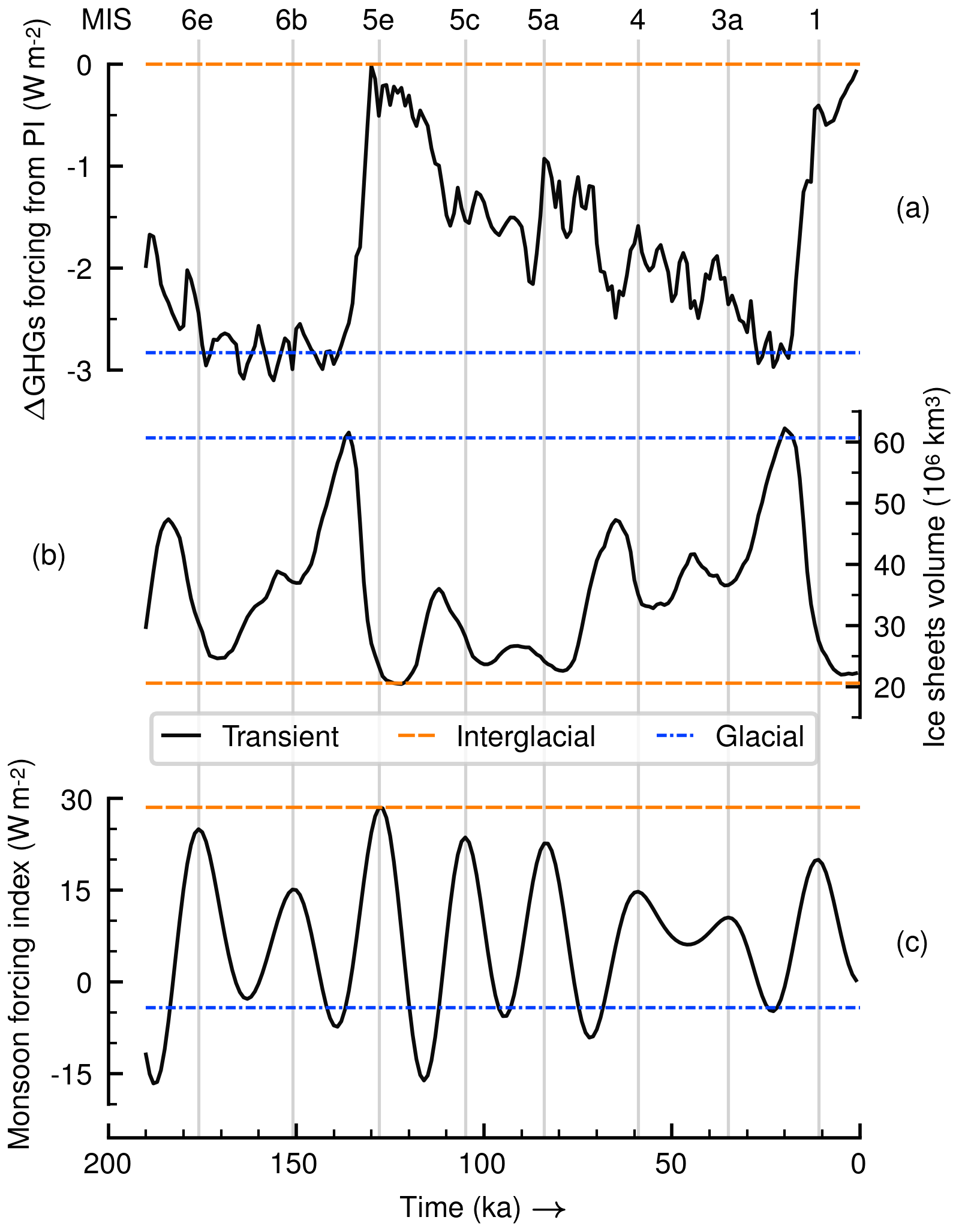
Figure 1 Prescribed forcing parameters in simulations: (a) GHG radiative forcing change (Δ) from preindustrial (PI) era, (b) ice sheet global ice volume and (c) orbital forcing via the monsoon forcing index. Transient series come from Antarctic ice cores, modelled ice sheet data and orbital theory, respectively. Horizontal lines are cases when forcings are fixed to interglacial or glacial reference values. Vertical lines indicate maxima in the monsoon forcing index and are labelled using MIS names on top (see Appendix A for details about notation).

2.2 Experiments of past AHPs

We simulate the coupled atmosphere, ocean, sea ice, land surface and vegetation dynamics for the past 190 kyr. The polythermal ice sheets model and global carbon cycle model components are not employed since we prescribe ice sheet extent and atmospheric GHG levels using available data. Simulations start from an equilibrium state attained after a 5 kyr simulation that maintained parameters set at 190 ka values. We perform 15 transient simulations prescribing possible combinations of climate forcing factors: GHG levels, ice sheet extent and orbital parameters. Forcings are prescribed either with a transient series from past evidence or with a single reference value as shown in Fig. 1. Reference values are taken from the transient series close to the Eemian interglacial state at about 125 ka and close to the Last Glacial Maximum (LGM) at about 21 ka. The GHG radiative forcing change from preindustrial (PI) conditions in Fig. 1a comes from Ganopolski and Calov (2011), and it considers variations in gases, CO₂, CH₄ and N₂O, that are in line with Antarctic ice cores (Petit et al., 1999; EPICA Community Members, 2004). Ice sheet data are model output from a simulation also in Ganopolski and Calov (2011) which agrees with sea level changes in Waelbroeck et al. (2002) and the reconstructions of Peltier (1994). Ice sheets are represented by a spatially distributed transient series varying mostly in the Northern Hemisphere, even though we show only the global cumulative ice volume (Fig. 1b). The Earth's orbital parameters (precession, obliquity and eccentricity) vary according to Berger (1978). We show their secular variations using the monsoon forcing index defined by Rossignol-Strick (1983), which measures an insolation gradient in the tropics relevant to monsoon systems and AHPs (Fig. 1c). In the text and in Fig. 1 we label peaks in the monsoon forcing index using MIS names to ease location of time slices when AHPs usually occur. Details about forcings, computation of the monsoon forcing index and MIS nomenclature are given in Appendix A.

Berger (1978)Berger (1978)Berger (1978)Berger (1978)Berger (1978)Berger (1978)

Table 1 Experiments and forcing settings. Entries in the “Field” column indicate how a climatic variable taken from an experiment is used in the factor separation method (see Appendix B with equations). Transient series are those in Fig. 1. The future set is not part of the separation method; 0 ka is present day, and kyr AP is millennia after present day.

Experiments of past AHPs and their forcing setup combinations follow the factor separation method of Stein and Alpert (1993) for three factors: (1) GHG radiative forcing changes from the PI era, (2) ice sheet extent and (3) orbital parameters. Using this method it is possible to estimate individual (also called “pure”) and synergistic contributions of the forcing factors to a simulation outcome (or predicted climatic field). The method assumes all contributions are additive and can be separated subtracting fields of a set of sensitivity simulations. To implement the method, a specific simulation target must be chosen in order to calculate deviations from a baseline or control state (i.e. the factor separation depends on the target or point of view). We are interested in knowing how much the forcings contribute to the simulation of AHPs. We choose two simulation targets with opposing global climates and AHP situations: the Eemian interglacial at around 125 ka (i.e. warm global climate) with a strong AHP and the LGM at around 21 ka (i.e. cold global climate) with no AHP. Experiments and forcing combinations are shown in Table 1. Only in the control experiment E0 do all forcings vary realistically as in the transient series obtained from past data (see Fig. 1). For the rest of the experiments we have two sets of simulations using the interglacial or glacial reference values shown in Table 1, with all possible “fixed-or-transient” combinations in each set. For instance, simulation EI4 has both GHG forcing change and ice sheets fixed at the interglacial reference values for the entire 190 kyr run (i.e. they are kept constant at interglacial levels). Likewise for EG4 but instead the fixed values are the glacial levels. Experiments EI7 and EG7 have the three forcings fixed at their respective reference points. Details and equations of the separation analyses are given in Appendix B.

2.3 Experiments of future AHPs

The low computational cost of the model and information available about future changes in the forcings enable us to also look into potential future climate change in North Africa. We are also interested in knowing how much our findings from the past can inform the future. Additional simulations start from present-day conditions in the control experiment E0 and cover the next 100 millennia after present (kyr AP). Projections of GHG radiative forcing changes from the PI era are based on the CO₂ emissions scenarios of Archer and Brovkin (2008), which estimate possible cumulative amounts of carbon to be released to the atmosphere in units of gigatonnes of carbon (Gt C). The emission estimates take into account both data from the reports of the Intergovernmental Panel on Climate Change (IPCC) and the size of available coal deposits to designate “moderate” or “large” amounts. Six experiments include a scenario of null emissions since preindustrial conditions (0 Gt C); a moderate emissions scenario with a release of 1000 Gt C; a large emissions scenario with a release of 5000 Gt C; and the intermediate cases of 2000, 3000 and 4000 Gt C. In these scenarios 90 % of the emissions are assumed to occur within the first few centuries of simulation, meaning there is an early peak of atmospheric concentration of CO₂ that subsequently decays to an equilibrium value (higher than preindustrial). These experiments are also shown in Table 1. For these simulations we ignore the radiative forcing effect of other GHGs. The orbital forcing is considered to continue changing following Berger (1978). We keep the ice sheets fixed at the preindustrial setting, neglecting the effects of a potential complete deglaciation or a new glacial inception. The latter is justified since a large ice sheet should not emerge within the next 100 kyr, even for the moderate emissions scenario (Ganopolski et al., 2016).

3 Results

We study century-mean values of model output for near-surface air temperature, daily precipitation and fractional vegetation coverage in the Sahara region. In the model the Sahara is a single grid box spanning approximately 20–30^∘ N and 15^∘ W–50^∘ E. We present astronomical season averages of summer (June–July–August) and winter (December–January–February) for temperature and precipitation, which are resolved daily in the model, whereas for the vegetation cover fraction only annual mean values can be reported.

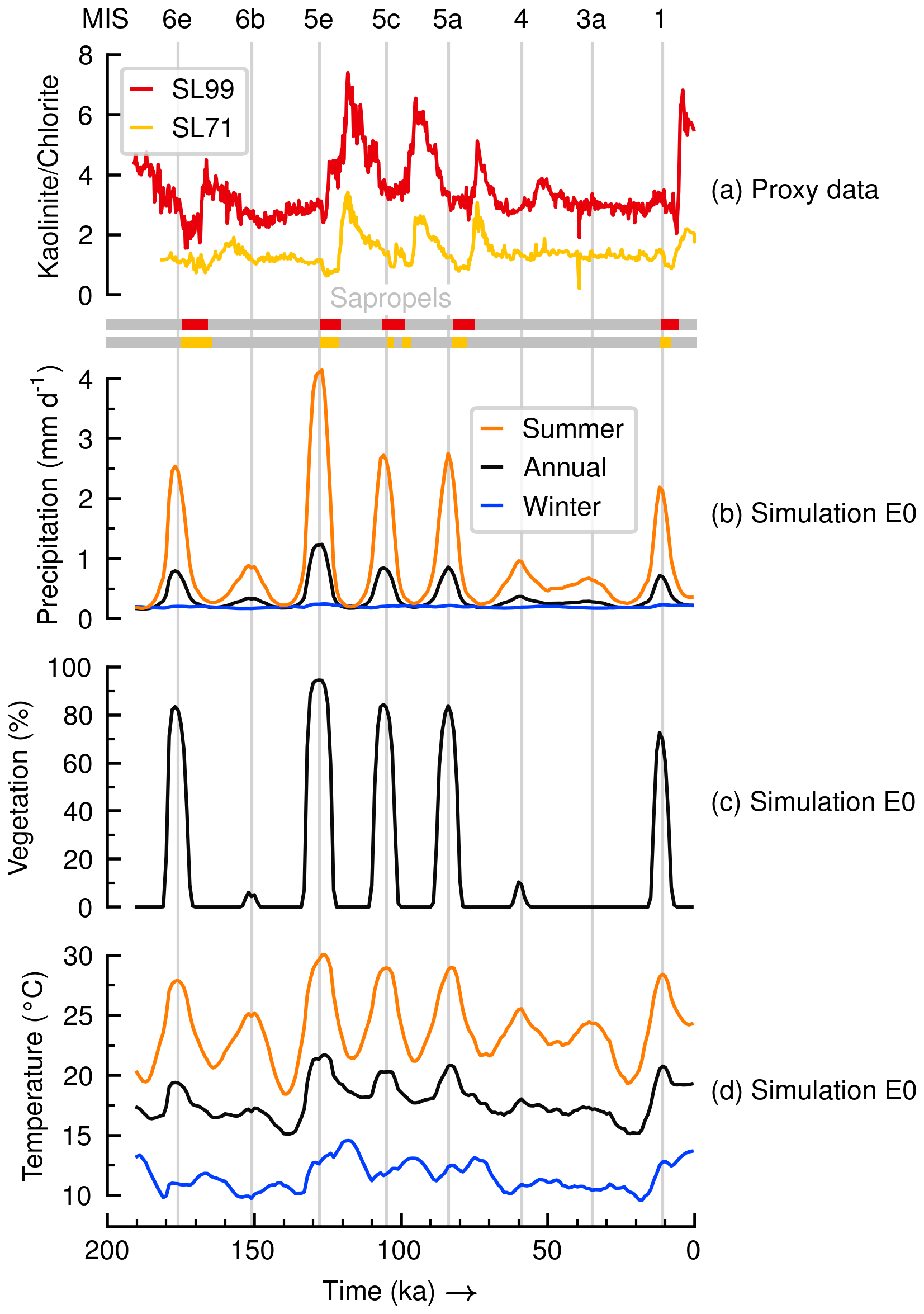
Figure 2 Comparison of (a) proxy data with (b, c, d) results from control simulation E0 in the Sahara grid box: annual and seasonal means of (b) precipitation, (c) vegetation cover fraction and (d) near-surface temperature. Proxy data are ratios of clay minerals and sapropel layers from sediment cores SL71 and SL99 from the eastern Mediterranean Sea described in Ehrmann and Schmiedl (2021). Vertical lines indicate maxima in the monsoon forcing index and are labelled using MIS names on top.

3.1 Simulation of past AHPs

Results of the control simulation E0 are shown in Fig. 2, alongside proxy data from sediment cores SL71 and SL99 from the eastern Mediterranean Sea (Ehrmann and Schmiedl, 2021). The proxies in Fig. 2a show pulses in the ratios of fine-grained minerals (kaolinite and chlorite), always found following a sapropel layer in the sediments. The sapropel doublet during MIS 5c for core SL71 corresponds to a single event in spite of the interruption in the sediments, which could be explained by postdepositional redox reactions (Grant et al., 2016). The sapropel layers indicate past instances of AHPs, when enhanced riverine discharge suppressed seabed oxygenation in the Mediterranean Sea, while the amplitudes of the dust pulses reveal the strength of the hydrological cycle during their preceding AHPs since the mineral production depends on rainfall intensity (weathering). In Fig. 2a the dust pulses lag the sapropel layers because aeolian dust transport from waterbodies across (most likely) North Africa can only occur once arid conditions are re-established after an AHP. The comparison between the proxy data and our simulations can only be qualitative in nature since we do not model either dust transport into the Mediterranean Sea or sapropel formation. It is remarkable, however, that the control simulation E0 (Fig. 2b–d) shows large peaks close in time with the sapropel layers in the proxies. Also in both simulation E0 and the proxies the strongest signals happen during MIS 5e. The simulation E0 is in closer agreement with the data from core SL71, where the pulses after MIS 5c and 5a have similar magnitude. Comparison with other proxy data from marine cores off the coasts of West Africa (Skonieczny et al., 2019) and East Africa (Tierney et al., 2017a) likewise reveals agreement in timing and in magnitude of the E0 simulation with the proxies (not shown).

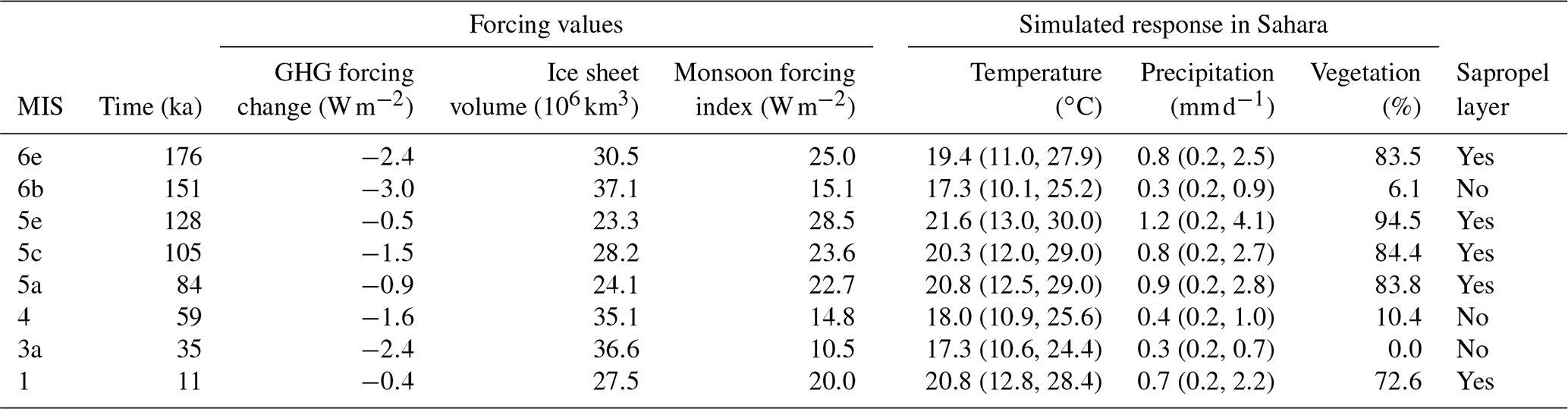
In Fig. 2 simulation E0 shows that peak values of precipitation, the vegetation cover fraction and temperature in the Sahara region coincide with peaks in the monsoon forcing index during the past 190 kyr. The peak values are summarised in Table 2. In the case of precipitation (Fig. 2b) and temperature (Fig. 2d) this is most conspicuous in the summer seasonal means, with large peaks similar to those evident in the vegetation cover fraction (Fig. 2c). The strongest peak values occur during the last two interglacial periods at MIS 5e and 1, as well as during MIS 6e, 5c and 5a. Only these five MIS periods have a vegetation cover fraction above 70 %. The vegetation peaks happen during warmer periods when annual mean daily precipitation is greater than 0.7 mm d⁻¹. This could accumulate to more than 250 mm yr⁻¹, well above the minimum limit estimated to support perennial grasslands and savanna biome types in North Africa (Larrasoaña et al., 2013). Although this precipitation value is low compared to estimates from proxy data (Braconnot et al., 2012), any amount over 200 mm yr⁻¹ is still distinctly greater than present-day values across the region (Bartlein et al., 2011) and is within the variability range of more sophisticated climate models for the last AHP during the Holocene (e.g. Harrison et al., 2015; Pausata et al., 2016; Dallmeyer et al., 2020). Therefore we consider these peak times to be simulated past AHPs with CLIMBER-2. The oldest one at MIS 6e was also found by Tuenter et al. (2005), and those at MIS 5c, 5a and 1 agree with the results of Tjallingii et al. (2008). Measuring from the moment the modelled vegetation starts growing until the moment it vanishes (Fig. 2c), the AHPs last on average 10.8 kyr, with the one at MIS 5e being the longest (12 kyr) and the one at MIS 1 the shortest (9 kyr).

Table 2 Forcing values and results in the Sahara grid box of seasonal and annual mean values in control experiment E0, taken near maxima of the monsoon forcing index. Sapropel layers are those in Fig. 2a. Values in parentheses are winter and summer means, in that order.

3.2 Correlation of forcings and AHPs

A first approximation to study the effects of the forcings on the modelled AHP response follows a simple linear regression analysis. With the values from Table 2 we plot paired combinations of forcings and response variables in phase diagrams and fit regression lines with the ordinary least-squares method and use the statistic R² and the p value of the F statistic as goodness-of-fit estimates. The forcings are included in the regression analysis (besides the modelled response) because even though we know that GHG levels and ice sheets are not independent from the orbital forcing, we do not know exactly how they relate to each other during AHPs. We also recognise that GHGs and ice sheets are global features, while the monsoon forcing index is a regional insolation gradient. We find there is a strong correlation (R²=0.75, p value=0.006) between the average ice sheet volume and the monsoon forcing index peaks, with the highest monsoon forcing index values having the least ice volume. In contrast, we see a weak correlation (R²=0.27, p value=0.19) between the GHG radiative forcing and the monsoon forcing index peaks.

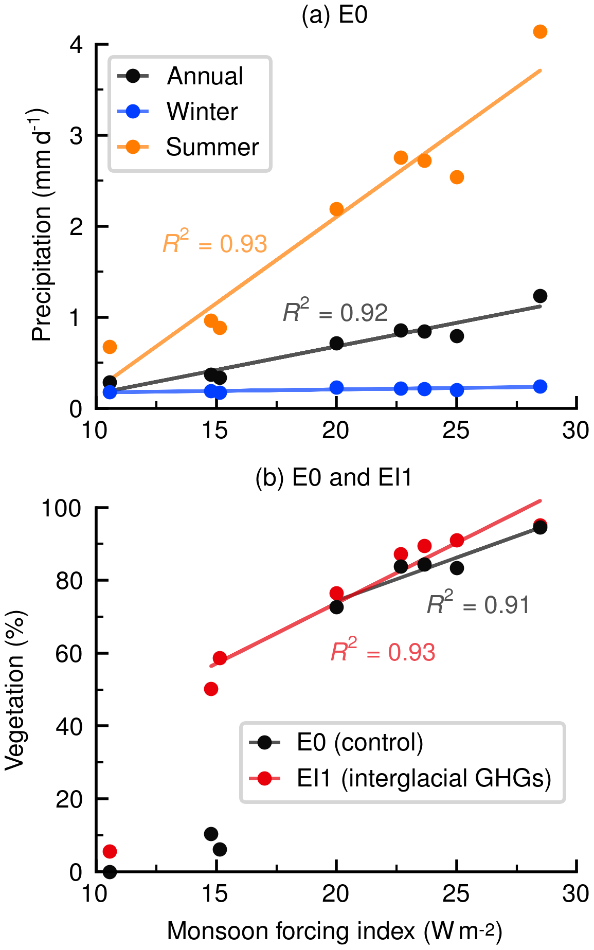
Figure 3 Correlation of the monsoon forcing index with the simulated response in the Sahara grid box in control simulation E0 for mean values of (a) precipitation and (b) vegetation cover fraction during peak times of the monsoon forcing index. Values of E0 are the same as in Table 2. In (b) we also include the modelled vegetation from experiment EI1 with fixed interglacial GHGs.

The modelled response correlates strongly with the monsoon forcing index during its peak times, as shown in Fig. 3. For precipitation (Fig. 3a) we observe a positive linear relationship for summer seasonal (R²=0.93, p value=0.0001) and annual (R²=0.92, p value=0.0001) means; therefore higher monsoon forcing index values yield higher precipitation in the Sahara grid box. Winter precipitation being almost a flat line shows this modelled variable in the Sahara does not depend on the monsoon forcing index. In the case of vegetation (Fig. 3b) we see non-linear behaviour with an abrupt large jump from low (about 10 %) to high (about 70 %) vegetation coverage within a small range of variation in the monsoon forcing index from around 15 to 20 W m⁻². In fact, for vegetation cover the change-point analysis of Killick et al. (2012) finds a change point (i.e. a significant jump in the linear regression) between values of the monsoon forcing index of 15 and 20 W m⁻². When applied to the correlation of precipitation with the monsoon forcing index, the change-point analysis does not find a jump in the linear regression at the same level of significance as for vegetation cover. Vegetation cover values occurring past the threshold range have a strong correlation (R²=0.91, p value=0.012) with the monsoon forcing index.

We also include in Fig. 3b the vegetation response of sensitivity simulation EI1 (with interglacial GHG forcing) because it shows that the insolation threshold might be sensitive to the GHG forcing. With interglacial GHG radiative forcing (experiment EI1) the threshold decreases below 15 W m⁻², and the correlation past this threshold between vegetation cover and the monsoon forcing index is still strong (R²=0.93, p value=0.0005). Looking also at the GHG radiative forcing values in Table 2 for MIS 6b and 4 (the points close to 15 W m⁻² in Fig. 3), we find that there is an average increase of about 2 W m⁻² in the GHG forcing in simulation EI1 relative to the control simulation E0. Hence we tentatively suggest that an increase in GHG forcing of some 2 W m⁻² is associated with a decrease in the threshold of the monsoon forcing index by some 5 W m⁻². This implies a sensitivity of the threshold in monsoon forcing index to a change in GHG forcing of around −2.5.

Existence of such threshold behaviour suggests that changes in the model should happen at a fast rate. Already in Fig. 2c we see that vegetation growth and decline phases occur rapidly. To look into the rates of change more carefully we plot in Fig. 4 the temporal derivatives of the forcings and the simulated vegetation fraction in the Sahara in the control experiment E0. This figure shows how the non-linear dynamics of the vegetation response does not follow smoothly the speeds of change in any of the forcings. However, vegetation growth and decline phases are coherent with times of increasing and decreasing rates, respectively, of the monsoon forcing index. In fact, we also find a strong correlation (R²=0.96, p value<0.0001) between peak speeds of change in the monsoon forcing index and peak growth and decline rates of the vegetation response. The fastest vegetation growth rate occurs during MIS 5e (59.2 % kyr⁻¹), when a peak in the increasing rate of the monsoon forcing index coincides with a relatively strong increase in the speed of change in the GHG radiative forcing and the strongest decline rate in the ice sheet volume. Figure 4d shows that the vegetation growth phases, during AHP onset, usually occur at faster rates than the decline phases during AHP terminations, which is most conspicuous during MIS 6e (onset at 50.1 % kyr⁻¹ versus termination at −31.6 % kyr⁻¹). Only during MIS 5a is this not the case (onset at 33.7 % kyr⁻¹ versus termination at −39.7 % kyr⁻¹), when ice sheets do not wane at a strong pace. On average, during AHPs the vegetation growth phase lasts about 5.2 kyr and the vegetation decline about 6.2 kyr.

3.3 Factor separation analyses

We suspect that differences in intensity amongst AHPs should be mainly determined by differences in the state of GHGs, ice sheets and orbital configuration at the time they occur. However, we do not know how much each of the forcings affects the AHP intensities. To look into this we perform simulations according to the factor separation method of Stein and Alpert (1993) and implement its equations (see Appendix B) using the model output for annual means of temperature, precipitation and the vegetation fraction in the Sahara region. Because the separation method depends on the chosen simulation target, we carry out two analyses: one of them isolates the contributions of the forcing factors to attain an Eemian-like strong AHP response (i.e. interglacial perspective), while the other one does it for an LGM-like non-AHP response (i.e. glacial perspective).

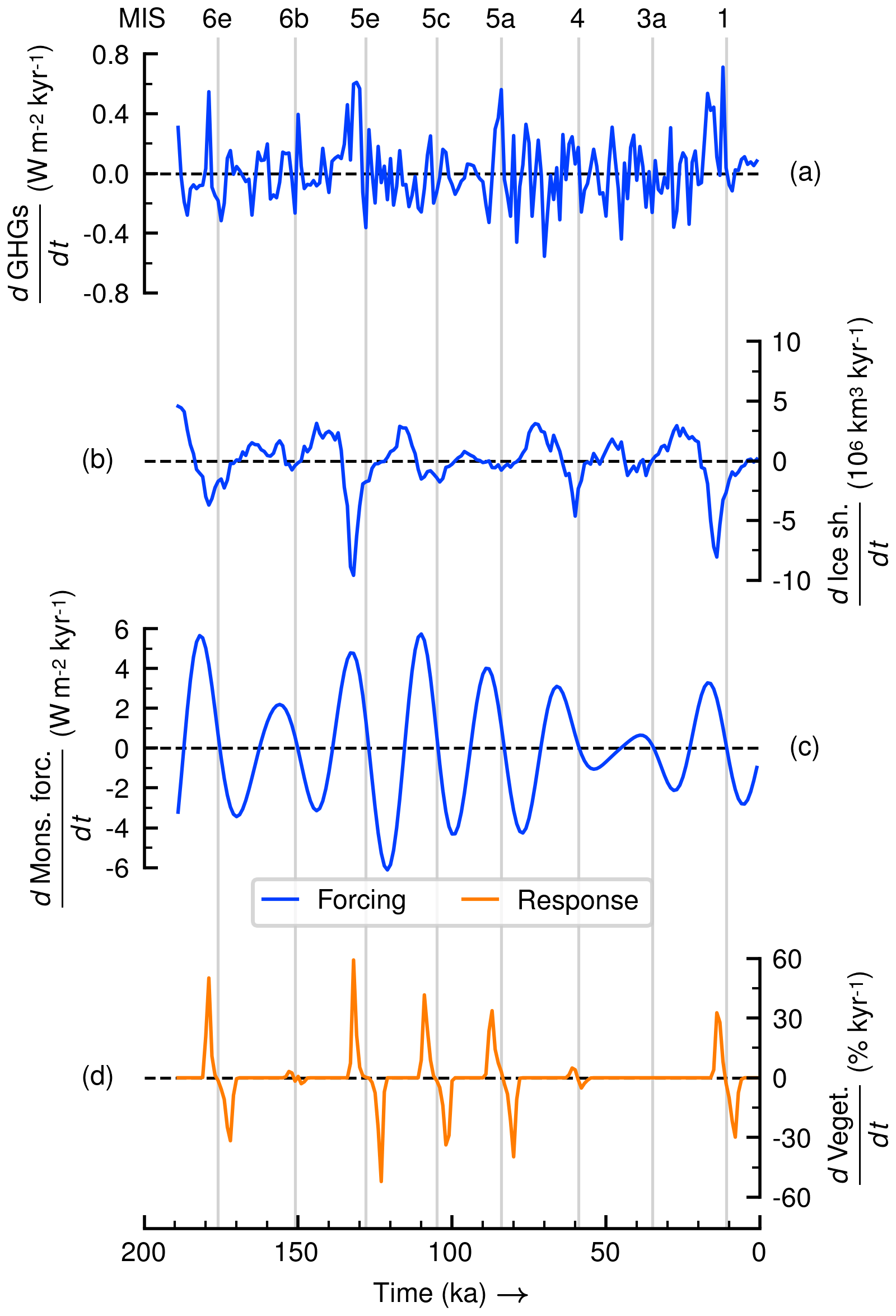
Figure 4 Rates of change of forcings and modelled response in control experiment E0: (a) GHG radiative forcing change from PI era, (b) global ice sheet volume, (c) monsoon forcing index and (d) simulated vegetation cover fraction in the Sahara grid box. Vertical lines show maxima of monsoon forcing index and are labelled using MIS names on top.

Both target responses for the two separation analyses are represented in simulations EI7 and EG7. Simulation EI7 from the interglacial perspective has all three forcing factors fixed at interglacial conditions (using the Eemian as reference). In this simulation, annual mean Saharan temperature stays for all times at 21.8 ^∘C, precipitation at 1.3 mm d⁻¹ and the vegetation cover fraction at 95.8 %. These values resemble those around the Eemian peak (about 125 ka) in the control simulation E0 (see Fig. 2). Simulation EG7 from the glacial perspective has forcings fixed at glacial conditions (using the LGM as reference). In this simulation, annual mean Saharan temperature remains for all times at 15.2 ^∘C, precipitation at 0.2 mm d⁻¹ and the vegetation cover fraction at 0.0 %. These values resemble those around the LGM (about 21 ka) in the control simulation E0 (see Fig. 2). Therefore, the interglacial-perspective experiment EI7 keeps a permanent strong Eemian-like AHP for the entire simulation, whereas the glacial EG7 keeps none. Through the factor separation method we then estimate how much each of the forcings is contributing at all times to the differences between the control experiment E0 and targets EI7 (strong AHP) and EG7 (no AHP).

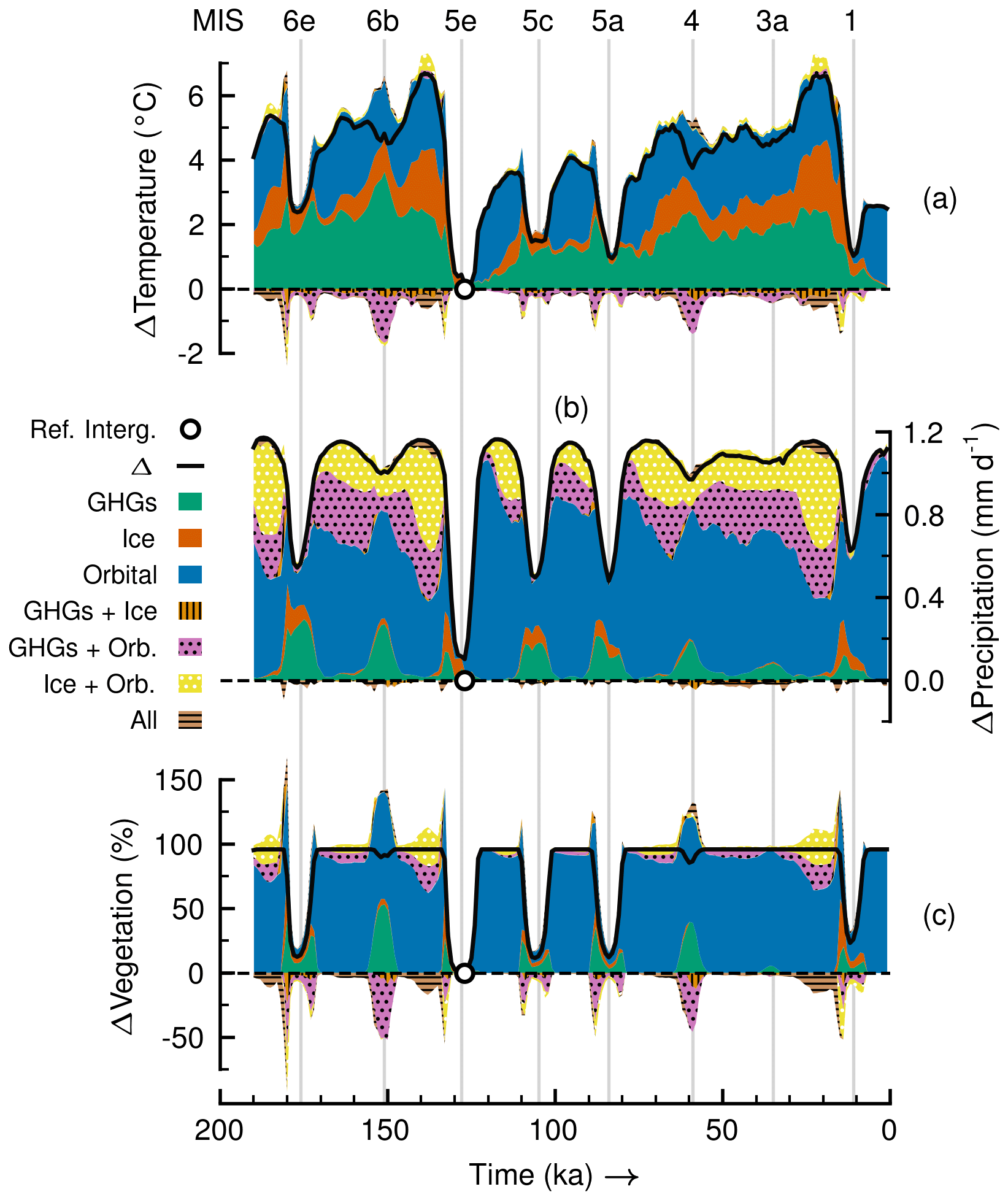
Figure 5 Factor separation analysis in the Sahara grid box from an interglacial perspective for annual means of (a) near-surface temperature, (b) precipitation and (c) vegetation cover fraction. Colours indicate contributions from individual forcings and related synergies to the total deviation in EI7 (Eemian-like AHP) from the control experiment (Δ= EI7 − E0). Synergies are also shown with patterns. A marker shows the location of the reference interglacial state, where the difference between EI7 and E0 is minimal. Vertical lines indicate maxima of the monsoon forcing index and are labelled using MIS names on top.

Results of the separation analysis from the interglacial perspective are shown in Fig. 5 for AHP temperature, precipitation and the vegetation cover fraction. With the forcing factors fixed at interglacial levels, the modelled response in EI7 (Eemian-like AHP) always deviates positively from the control experiment E0 for the three climatic variables. This is as expected since the resulting values of EI7 in the previous paragraph are higher than those in the control E0 at all times (only the Eemian in E0 is close to EI7). The slight offset between E0 and EI7 at MIS 5e occurs because the combination of prescribed forcings in EI7 happens closely around MIS 5e but not exactly at the same time during the control experiment E0. The relevant outcome of the separation method lies in the colours (and patterns) in Fig. 5, which show how the forcings contribute to the EI7–E0 difference. For AHP temperature (Fig. 5a) the individual contribution of each forcing is directly proportional to the change in the forcing. To see this it is necessary to compare differences between the control forcing values in the transient series in Fig. 1 and the interglacial reference level in that same figure. For instance, at MIS 6b the largest contribution to temperature change comes from the GHG radiative forcing change (Fig. 5a) since that is the forcing with the largest difference between the transient series and the interglacial horizontal line (see also Fig. 1a). For the AHP temperature response the synergistic effects are small in comparison to the individual contributions. Averaging the contributions to AHP temperature for the whole time series in Fig. 5a shows that GHGs add about 1.6 ^∘C (41.1 % of change from E0), ice sheets 0.8 ^∘C (19.9 % of change from E0) and the orbital forcing 1.8 ^∘C (45.9 % of change from E0). The synergy between GHGs and the orbital forcing is small but is the synergy with the largest effect, adding on average about −0.2 ^∘C (−4.9 % of change from E0).

The AHP precipitation case in the separation analysis is different to the temperature one. Figure 5b shows that the AHP precipitation response largely depends on the orbital forcing (substantial blue colour). Not only is the individual contribution of this forcing the largest for all times, but also its synergies with the other two forcings have relatively large effects. The individual contribution of the GHG radiative forcing to changes in AHP precipitation is small. The individual effects of ice sheets on AHP precipitation are negligible as well. No synergistic effects seem to exist between the ice sheet forcing and the GHG radiative forcing. Averaging the contributions to AHP precipitation for the whole time series in Fig. 5b, we find that GHGs add about 0.1 mm d⁻¹ (6.7 % of change from E0), ice sheets close to 0.0 mm d⁻¹ (2.2 % of change from E0) and the orbital forcing about 0.6 mm d⁻¹ (59.3 % of change from E0). Both synergies of the orbital forcing with GHGs and ice sheets round up to 0.2 mm d⁻¹ (each about 15 % of change from E0). This means the effects of the orbital forcing and these two synergies with GHGs and ice sheets amount to about 90.9 % of the change from E0.

AHP vegetation results in Fig. 5c are similar to the AHP precipitation case, although the individual effect of the orbital forcing is much more conspicuous (predominant blue colour). The negative synergistic effects seen in the vegetation changes should be an artefact of the separation analysis method because vegetation is a bounded quantity. Consider, for example, the time around 150 ka during MIS 6b, when the Sahara is much greener, close to a 100 % vegetation cover, in simulation EI7 than in simulation E0 (Fig. 5c). The individual contribution of orbital forcing (blue colour) would make some 90 % of the Sahara green and the GHG forcing (green colour) some 50 %. If both forcings are active, then the pure contributions cannot be superposed (do not add linearly) because the Sahara cannot be more than 100 % covered with vegetation. Therefore, the synergy between these forcings (pink colour and dot pattern) has to be negative. Average contributions to AHP vegetation for the whole series in Fig. 5c are about 5.8 % from GHGs (6.4 % of change from E0), 2.2 % from ice sheets (2.4 % of change from E0) and 72.6 % from the orbital forcing (79.5 % of change from E0). The synergy (when positive) between GHGs and orbital forcing adds on average about 4.0 % (4.4 % of change from E0) and the synergy (when positive) between ice sheets and orbital forcing about 5.3 % (5.8 % of change from E0). The orbital forcing and all of its synergies account for about 90.4 % of vegetation change from E0.

From the glacial perspective in the additional separation analysis, we do not find anything significantly new; hence details are to be found in Appendix C. Figure C1 shows that in this case the deviations in EG7 from the control E0 are always negative for the three climatic variables and the effects of the ice sheet changes are larger than those of the GHGs. Nonetheless, the same behaviour for temperature is observed, with changes being proportional to the changes in the forcings. This analysis demonstrates that it is the relatively low maxima in orbital forcing that result in the absence of AHP conditions at MIS 6b, 4 and 3a – rather than the low GHG radiative forcing or the large ice sheets. From this perspective synergies are more difficult to assess because of the lower bounds in precipitation (0 mm d⁻¹) and the vegetation cover fraction (0 %).

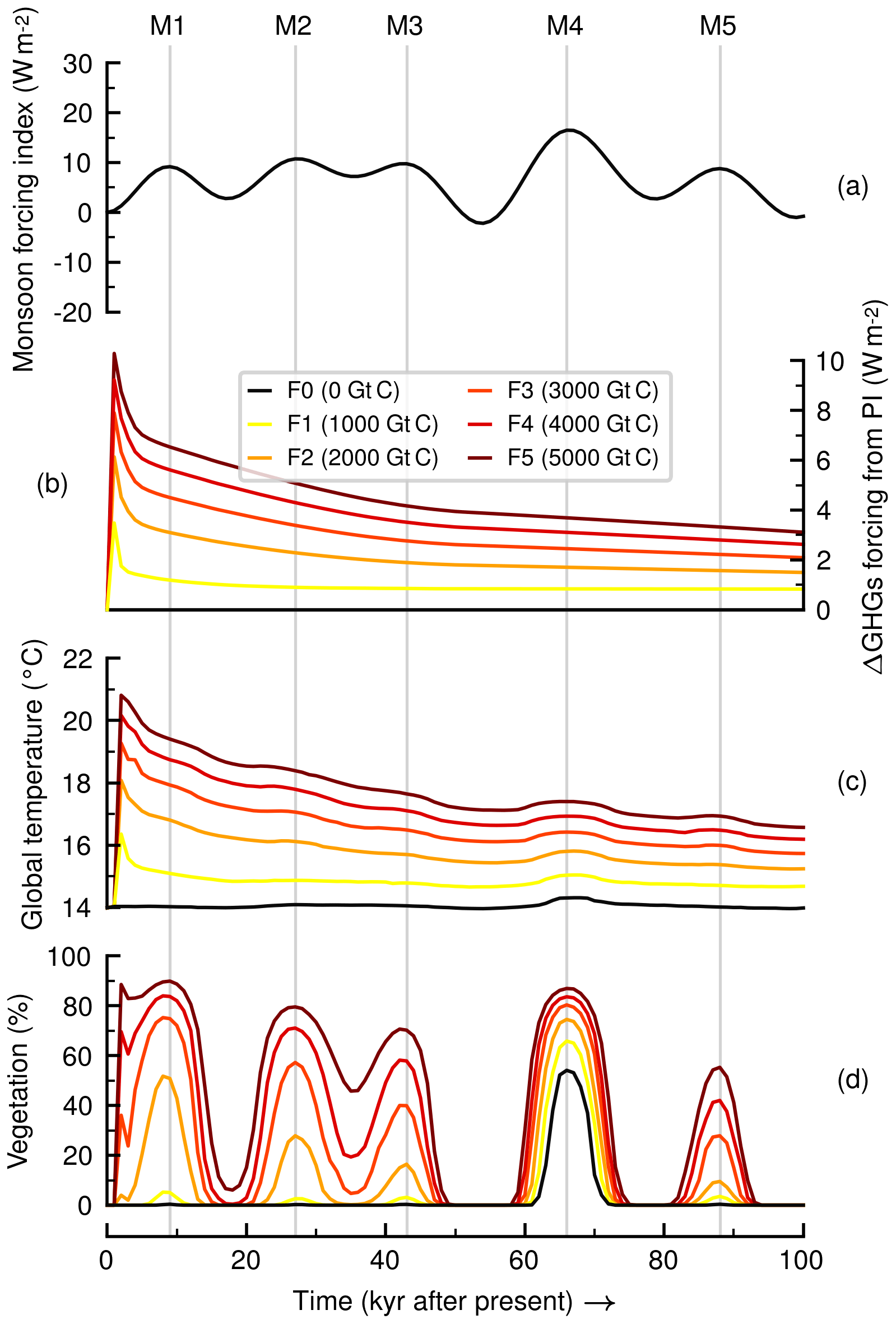
Figure 6 AHPs in future climate change scenarios for the next 100 kyr: (a) computed monsoon forcing index, (b) scenarios of GHG radiative forcing changes from PI era, (c) simulated global near-surface temperature and (d) modelled vegetation fraction in the Sahara grid box. Vertical lines indicate future peaks in the monsoon forcing index. Total cumulative emissions of carbon are shown in parentheses in the legend.

3.4 AHPs in scenarios of future climate change

When computing the monsoon forcing index for the next 100 kyr (millennia after present) we see that the onset threshold range of past AHPs (15–20 W m⁻² in the model) will not be crossed within the next ca. 60 kyr (Fig. 6a). The amplitude in the monsoon forcing index (proxy for orbital forcing) is much smaller than that of past times (see Fig. 1) due to low eccentricity in the Earth's orbit. Only for the time around 66 kyr AP does the monsoon forcing index approach the onset threshold range. From the sensitivity simulation EI1 in which the GHG radiative forcing change is set to an interglacial level, we find that an increase in GHG forcing by some 2 W m⁻² can lower the threshold in the monsoon forcing index by some 5 W m⁻² (Fig. 3b). Hence we expect that in a climate with much stronger GHG forcing and much warmer global temperatures (Fig. 6b and c), the threshold might decrease even further. The simulations F0–5 corroborate the lesson learnt from the study of the past; Fig. 6d shows AHP responses for monsoon forcing indices below 10 W m⁻².

The modelled vegetation response in Fig. 6d shows the potential effects of increased GHG radiative forcing for climate in the Sahara. The no-emissions scenario F0 (0 Gt C) predicts that no AHP should occur before the next 60 kyr. For this scenario only at 66 kyr AP (named peak M4) is the threshold range of the monsoon forcing index crossed slightly at 16.5 W m⁻², and we see a vegetation response of about 54.1 %. However, for the moderate emissions scenario F1 (1000 Gt C) we see already that additional vegetation responses begin to occur at earlier monsoon forcing index peaks. These are still quite small responses since the average change in GHG radiative forcing stays close to 1 W m⁻² for this scenario, and according to our estimate from the past simulations, this means the threshold range only decreases by 2.5 W m⁻² from its original position at 15–20 W m⁻²; thus it remains higher than most peaks in the monsoon forcing index in Fig. 6a. Such mild responses are amplified as the GHG radiative forcing increases with the other scenarios. For instance, for the large emissions scenario F5 (5000 Gt C) the vegetation cover response at 9 kyr AP (peak M1) with a monsoon forcing index of only 9.2 W m⁻² is already at about 89.9 %, which is higher than that of the strongest monsoon forcing index peak M4 for any scenario. In this case the average GHG forcing change is close to 6 W m⁻², which according to our calculations should lower the threshold range in the monsoon forcing index to about 2–7 W m⁻² (lowered by 13 W m⁻²), and this would explain why with only 9.2 W m⁻² of the monsoon forcing index do we see such a strong response. Therefore we see that the effect of the large GHG radiative forcing in the early 60 kyr AP of simulation is compensating for the low monsoon forcing index values during this time. Nonetheless, this effect is only seen at the monsoon forcing index peaks; therefore the orbital forcing is still the triggering mechanism for the AHP response.

4 Discussion

Our aim is to quantify the effects of multiple forcings on the simulated vegetation cover in the Sahara region during AHPs. To this end we use CLIMBER-2, a climate system model of intermediate complexity. CLIMBER-2 runs at a coarse resolution with three grid cells representing North Africa: the Sahara, the Sahel and tropical North Africa. CLIMBER-2 is a statistical–dynamical model in which the effect of weather on climate is parameterised. Hence CLIMBER-2 does not reveal any variability at decadal timescales and shorter. This implies that CLIMBER-2 cannot be used to study the role of decadal internal variability on AHPs, which might play an important role during transition phases (e.g. Liu et al., 2006; Bathiany et al., 2012; Brierley et al., 2018). Despite these limitations, CLIMBER-2 has proven a useful tool in many studies of large-scale climate processes at timescales of centuries to millions of years, including the first transient simulations of abrupt vegetation changes in Africa (e.g. Claussen et al., 1999b, 2003).

We begin by re-assessing the ability of CLIMBER-2 to simulate past occurrences of AHPs during glacial–interglacial cycles. Our results broadly agree with previous efforts which also found the model's performance adequate (e.g. Tuenter et al., 2005; Tjallingii et al., 2008). Magnitude and timing of the simulated AHPs compare favourably not only with the proxy data in Tierney et al. (2017a), Skonieczny et al. (2019), and Ehrmann and Schmiedl (2021) but also with the data and simulations of Blanchet et al. (2021) and Kutzbach et al. (2020). Although comparison between simulations is limited due to large differences in spatial resolution, one difference that might be discussed is the magnitude of the simulated Holocene AHP. In the case of Blanchet et al. (2021) the AHP during the Holocene is stronger than those at MIS 5c and 5a. Our simulations show the opposite, in agreement with the simulations in Kutzbach et al. (2020). To reconcile this we can look at the sediment records from the Mediterranean Sea discussed in Ehrmann and Schmiedl (2021) and say that simulations of Saharan climate in CLIMBER-2 evolve like the proxy data from semi-distal sites off the North African coastline, whereas those in Blanchet et al. (2021) resemble the data from proximal sites. Spatial heterogeneity of the changes during AHPs hinders model consistency with all proxy data. Nevertheless our simulations show a reasonable representation of the evolution of the climate in the Sahara during the last 190 kyr, and this enables us to study the effects of forcing from GHGs, ice sheets and orbital parameters.

Analysis of our control simulation reveals that the AHP response in CLIMBER-2 is strongly correlated with the variations in the monsoon forcing index (proxy for orbital forcing based on a gradient in tropical insolation). This correlation was also found in the proxy data of Rossignol-Strick (1983) and Ehrmann et al. (2017). We find that there is a critical value of the monsoon forcing index that must be crossed to simulate Saharan greening with the model. Past this threshold vegetation and precipitation feed back through biogeophysical changes (see Sect. 2.1) and the climatic response in Sahara is amplified, resulting in an AHP (Brovkin et al., 1998; Claussen et al., 1999b). The amplification effect of the vegetation is clearly shown for this model in the sensitivity experiments of Claussen et al. (2003). Such non-linear responses from monsoon regions are also seen in proxy data (e.g. Rossignol-Strick, 1983; Ziegler et al., 2010). The threshold value we find lies somewhere between 15 and 20 W m⁻²; thus we refer to it rather as a threshold range. Depending on the strength of additional factors (such as GHGs or ice sheets) the critical value could be closer to the lower or the upper boundary of this range. Below 15 W m⁻² until about 10 W m⁻² the model simulates only a weak vegetation response that cannot develop into an AHP, probably because within this range the amplifying feedback between vegetation and precipitation is not yet effective. Rossignol-Strick (1983) found that the threshold for occurrence of sapropel layers in sediment cores from the Mediterranean Sea (an indication of past AHPs) is about 19.8 W m⁻² (41 Ly d⁻¹). How close this value is from the estimate from CLIMBER-2 is useful as additional validation for the model, even though we simulate Saharan greening and not sapropel formation.

From the control simulation we also find that the maximum onset and termination speeds of the AHP vegetation response correlate well with the speed of change in the monsoon forcing index. However, for the fastest rates of vegetation change to occur it is also important that the trends of change in the ice sheets and the GHG radiative forcing are favourable. For instance, at AHP onset during MIS 5e (fastest vegetation growth rate) the three forcing factors are synchronised with an increasing monsoon forcing index, strong reduction in ice sheets and an increasing rate of warming from GHG radiative forcing change. Synchronisation of the forcings may also explain why we find that vegetation growth speeds during AHP onsets are generally faster than those of vegetation decline during AHP terminations. Such difference between onset and termination speeds was also suggested for the Holocene AHP in Shanahan et al. (2015). Because of a lag in the ice sheet rate of change with respect to the orbital forcing change and because of the rather erratic rate of change of the GHGs, the three forcing factors are not usually coherent during AHPs terminations, resulting in slower vegetation rates of change (than those during AHP onsets). The only AHP termination that has faster vegetation changes than its onset occurs in MIS 5a, when a strong increase in ice sheets happens closely after the monsoon forcing index negative peak rate of change. In Lézine et al. (2011) the role of groundwater is described to explain why there is a rapid climate response during AHP onset and a subsequent slower more gradual AHP termination (with aquifers providing base flow). However, the model's hydrology does not include this feature, and we focus only on the speeds of the forcings and their synchronisation.

We complement the study of the control simulation with a factor separation analysis. Its outcome confirms the dominant role of the orbital forcing in setting the amplitude of the modelled precipitation and vegetation responses of past AHPs. This was already described, for instance, in Tuenter et al. (2003), Kutzbach et al. (2020) and Blanchet et al. (2021). In particular, a factor analysis in Blanchet et al. (2021) showed that the individual roles of the GHG radiative forcing and the global ice volume are of secondary importance for the strength of simulated AHPs. What we do with the factor separation method is make quantitative estimates of the said dominance or secondary importance of these forcings. From our results, when we add together the individual contributions from GHGs and ice sheets to the AHP precipitation or vegetation coverage responses, we find they amount to less than 20 % of the change induced by the orbital forcing alone. In fact, according to the simulations the orbital forcing alone (without effects from GHGs and ice sheets) should account for about 60 % (80 %) of changes in the AHP precipitation (vegetation cover) during the last 190 kyr. If its synergies are included, then the orbital forcing is responsible for more than 90 % of precipitation and vegetation changes. The factor separation also shows that GHGs and ice sheets have a larger impact on precipitation (and vegetation extent) when in synergy with the orbital forcing than individually. For near-surface temperature, in contrast, all the three forcing factors have a large effect individually and the synergies are all small in comparison.

But besides the dominance of the orbital forcing, the experiments of the factor separation method also reveal that the GHG forcing has important consequences for the existence of the threshold behaviour in the Sahara greening in the model. Our results suggest that an increase in GHG radiative forcing of some 1 W m⁻² can lower the threshold in the monsoon forcing index by some 2.5 W m⁻². We explain this reduction by the fact that both GHGs and orbital forcings tend to amplify precipitation and greening. Hence, with higher GHG levels the system responds earlier to a smaller orbital forcing. This has been demonstrated by, for instance, sensitivity experiments in Claussen et al. (2003) also using CLIMBER-2. They show how CO₂ and orbital forcings affect dynamic and thermodynamic contributions to Saharan precipitation. D’Agostino et al. (2019) also looked into these contributions in experiments of the Coupled Model Intercomparison Project phase 5 and arrived at a similar result. To understand how GHG radiative forcing changes can alter the threshold in orbital forcing, we look at the precipitation–vegetation feedback mechanism in the model (Claussen et al., 1999b). There is a minimum of Saharan vegetation (or precipitation) after which the precipitation–vegetation feedback sets in. With dynamic (circulation) effects alone, caused mainly by the changes in orbital parameters, the minimum triggering value of vegetation (or precipitation) is only reached when the monsoon forcing index is strong enough. However, when thermodynamical effects become stronger (increased GHGs, increased atmosphere warming, increased water vapour), the minimum value of vegetation (or precipitation) can be reached sooner or with a lower value of tropical insolation.

We take this lesson from the simulation of the past, about the relationship between GHGs and the threshold in orbital forcing, to evaluate the potential for future occurrences of humid periods. During the next 100 kyr the effects of changes in GHG radiative forcing become larger while those of the orbital forcing become weaker. The future of the ice sheets is more uncertain, but a glacial inception is not likely to happen (Ganopolski et al., 2016), and if we ignore potential catastrophic consequences of a complete deglaciation, the impact of the ice sheets on AHPs should not change much from its current interglacial-like effect. The main finding is that the GHG radiative forcing has an amplification effect on the simulated vegetation response that is large enough to overcome the limiting threshold for Sahara greening imposed by the orbital forcing. An alternative interpretation is that the GHG forcing lowers the tropical insolation requirement for AHP onset. Here it is also important to mention that we are neglecting biogeochemical effects since we prescribe GHG levels; therefore potential effects of feedbacks between the carbon cycle and vegetation are being ignored. The AHP responses are still paced by precession variations, but the increased atmospheric moisture (product of GHG radiative warming) compensates for a weaker gradient in insolation (i.e. lower monsoon forcing index).

5 Conclusions

We have used the climate model of intermediate complexity CLIMBER-2 to assess the role in AHP strength of three climate forcing factors: (1) Earth's orbital parameters, (2) GHG radiative forcing changes from preindustrial conditions and (3) ice sheet extent. Consistently with previous studies we find the model simulates reasonably well the evolution of past AHPs in terms of timing and magnitude. A newly discovered feature is the model contains the threshold behaviour of AHPs associated with the orbital forcing, previously found in proxy data. For the Saharan greening response during past AHPs, the simulated threshold in the monsoon forcing index lies within the range 15–20 W m⁻². Besides this critical threshold range, the monsoon forcing index also correlates well with the simulated precipitation and vegetation cover responses during AHPs, not only with their magnitudes but also with their rates of change: higher monsoon forcing index values lead to larger and faster changes. We also show that for fast changes to occur it is important that the rates of change of the forcings are synchronised. In the experiments this happens more often during AHP onset than termination, and therefore the onset vegetation rate of change is generally faster.

In addition to the results from a control experiment we include two complete factor separation analyses that make explicit the dominant role of the orbital forcing in setting the strength of past AHPs. The individual effects of the GHGs and ice sheets put together cause less than 20 % of the change induced by the orbital forcing. The effects of GHGs and ice sheets are notably greater when in synergy with the orbital forcing than separately. When we add together the effects of the orbital forcing and its synergies, it amounts to over 90 % of the change in the AHP precipitation and vegetation cover responses. Despite the dominance of the orbital forcing, when we extend the simulations to cover the next 100 kyr, we see that increased GHG radiative forcing indeed lowers the critical value of the monsoon forcing index that must be crossed to simulate Saharan greening and the subsequent AHP response.

These findings both support previous research and contribute new insights to our understanding of AHP dynamics. In several cases we are able to extrapolate previous knowledge from the Holocene AHP to earlier humid periods. In general the results agree with the consensus on predominance of the orbital forcing and make explicit the minor role that additional forcing from GHGs and ice sheets played during previous AHPs. However, because we consider both past and future simulations of AHPs, we are able to show that GHGs may be more important than previously thought. A key message from this work is that even though the orbital forcing is the leading factor setting intensity and timing of AHPs, the atmospheric levels of GHGs have the potential to lower the insolation requirement for AHP onset. We estimate the effect of the GHGs on the orbital forcing as a reduction of roughly 2.5 W m⁻² in the monsoon forcing index threshold range per 1 W m⁻² change in the GHG radiative forcing. Such an effect of GHGs in the past might have been hidden by the strength of the non-linear response to the orbital forcing, combined with a relatively narrow range of GHGs variability, yet it may be particularly important when considering future occurrences of AHPs under climate change scenarios.

Appendix A: Forcings, monsoon forcing index and MIS notation

Experiments with CLIMBER-2 differ only in the input data concerning the GHG radiative forcing changes from preindustrial conditions, the extent of ice sheets and the orbital parameters (precession, obliquity and eccentricity). The GHG radiative forcing input series agrees with data from Antarctic ice cores (Petit et al., 1999; EPICA Community Members, 2004). It is described in Ganopolski et al. (2010) as an equivalent CO₂ concentration (C_e) that includes variations in CO₂, CH₄ and N₂O. The total GHG radiative forcing change from the preindustrial era (ΔRF) is computed as

$$\begin{array}{}\text{(A1)}& \mathrm{\Delta }\mathrm{RF}=\mathrm{5.35}\ln {\displaystyle \frac{C_{\mathrm{e}}}{C_{\mathrm{0}}}},\end{array}$$

where C₀ is set to 280 ppm. The reference values for glacial and interglacial conditions are about 165 and 280 ppm of equivalent CO₂, respectively, which translate using Eq. (A1) into the radiative forcing values summarised in Table 1.

In the case of ice sheets, Fig. 1 shows only a global cumulative sum. For our simulations the input for the model is a gridded time series that is itself model output from an earlier simulation by Ganopolski and Calov (2011), who ran the CLIMBER-2 model employing the ice sheets model component SICOPOLIS (Greve, 1997). The ice sheet evolution is in agreement with the sea level change data from Waelbroeck et al. (2002) and the ice sheet maps of Peltier (1994). The reference values in this case are actually maps taken from the gridded series during the Eemian around 124 ka and the LGM around 21 ka. Their global cumulative ice volumes are those seen in Table 1. Sea level change corresponding to the Eemian ice sheet map is −0.21 m, while that of the LGM is −106.44 m.

Berger (1978)Berger (1978)Berger (1978)Berger (1978)

Table A1 Orbital parameters in CLIMBER-2 simulations and their respective monsoon forcing index value.

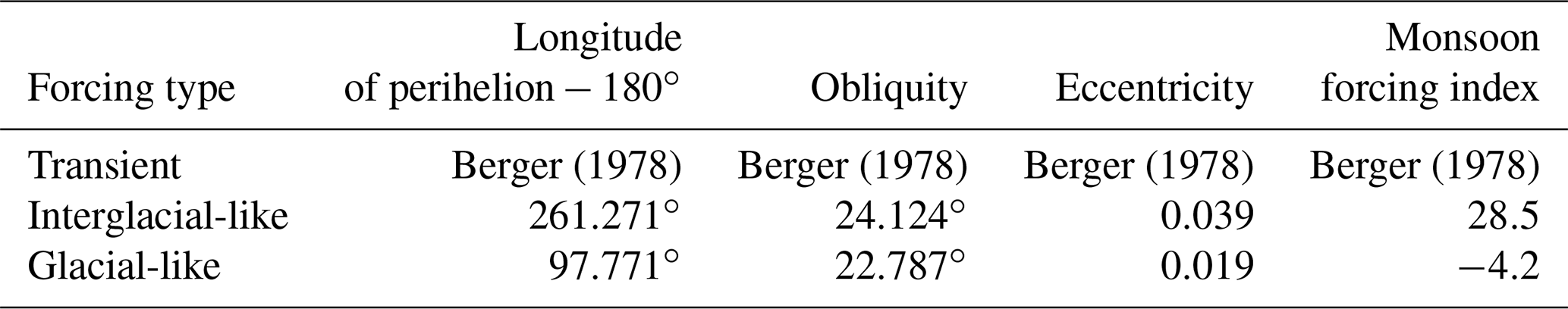
CLIMBER-2 by default computes the orbital parameters using the formulae of Berger (1978). In the experiments with fixed orbital forcing, we switch off the module for the Berger (1978) computation and fix the values of precession (setting the angle from vernal equinox to perihelion), obliquity and eccentricity to those calculated for the Eemian and LGM periods. These values are shown in Table A1. To summarise them into a single value, we use the monsoon forcing index defined by Rossignol-Strick (1983). To compute the index, it is necessary first to compute the cumulative insolation during the Northern Hemisphere caloric summer season defined by Milankovitch (1941). We do this using the daily insolation values computed with the Berger (1978) theory (to obtain astronomical seasons) and the equations presented in Vernekar (1972). The caloric summer insolation is obtained for latitudes at the Northern Tropic near 23.45^∘ N (I_T) and at the Equator (I_E), and then the monsoon forcing index (MI) at millennia before the present-day time slice t is

$$\begin{array}{}\text{(A2)}& {\mathrm{MI}}^t=\mathrm{2}{I}_T^t-I_E^t.\end{array}$$

Figure 1 shows in fact the variations in the monsoon forcing index from the 1950 Common Era (CE) reference value of about 482 W m⁻² (around 995 Ly d⁻¹). Because AHPs usually occur at peak times of this index, it is convenient for the discussion to be able to identify every monsoon forcing index maximum. Therefore, to label them we use the Marine Isotope Stage (MIS) name that occurred at the time of the monsoon forcing index maximum. This is also useful because MIS names give hints about the state of the climate system at the time. In spite of there not being consensus in some of the names, here we make use of the notation scheme put forth by Railsback et al. (2015). Figure A1 shows the monsoon forcing index in the control experiment and the Lisiecki and Raymo (2005) dataset used by Railsback et al. (2015). In Fig. A1 a thin bar with coloured boxes shows the different periods they identified. Vertical lines then help us in choosing the names for each monsoon forcing index peak.

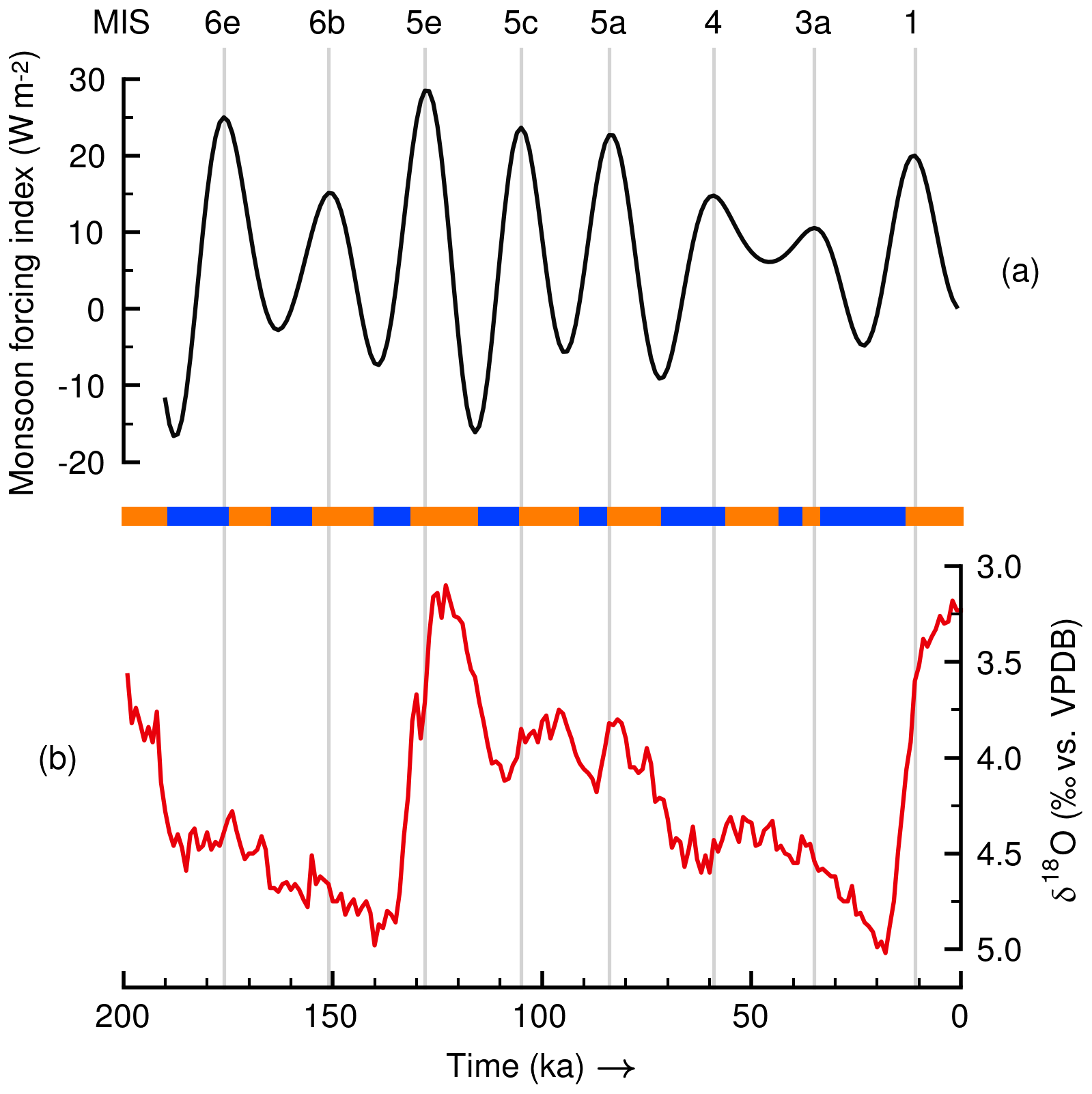
Figure A1 Notation for peaks of (a) monsoon forcing index using MIS labels on top, following the scheme in Railsback et al. (2015), who used the (b) Lisiecki and Raymo (2005) marine isotope stack data to label the time slices shown in a bar with different colours. The isotope data are with respect to the standard Vienna Peedee Belemnite (VPDB). Vertical lines indicate the monsoon forcing index peaks.

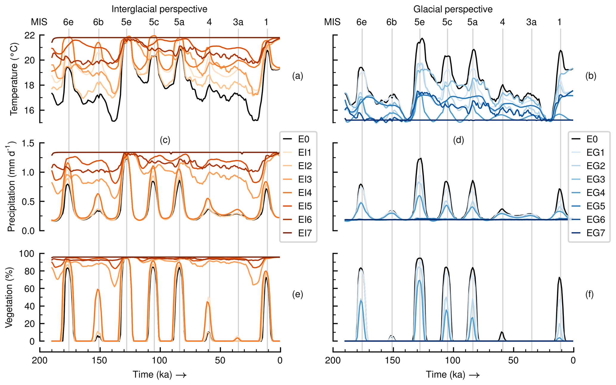
Figure A2 Results of annual means of (a, b) near-surface temperature, (c, d) precipitation and (e, f) vegetation cover fraction in the Sahara grid box for all simulations involved in the separation analyses from interglacial and glacial perspectives. Vertical lines indicate monsoon forcing index maxima and are labelled using MIS names on top.

Appendix B: Equations of separation analyses

We perform experiments following the separation method of Stein and Alpert (1993). In this case it is done for three factors: (1) GHG radiative forcing changes from the PI era, (2) global ice sheet volume and (3) orbital parameters. Consequently 2³ simulations are needed for one separation analysis. The technique uses deviations of a simulation target with respect to a baseline or control state (experiment E0). We choose two different simulation targets: (1) global interglacial conditions with a strong AHP and (2) global glacial conditions with no AHPs. The targets correspond to simulations EI7 and EG7, respectively. Therefore we undertake two separation analyses for AHPs: one from an interglacial perspective and the other from a glacial one. The equations for the separation analysis from the interglacial perspective are

$$\begin{array}{ll}\text{(B1)}& {\displaystyle }& {\displaystyle }{\widehat{f}}_{\mathrm{0}}=f_{\mathrm{0}},\text{(B2)}& {\displaystyle }& {\displaystyle }{\widehat{f}}_{\text{I, GHG}}=f_{\text{I, GHG}}-f_{\mathrm{0}},\text{(B3)}& {\displaystyle }& {\displaystyle }{\widehat{f}}_{\text{I, Ice}}=f_{\text{I, Ice}}-f_{\mathrm{0}},\text{(B4)}& {\displaystyle }& {\displaystyle }{\widehat{f}}_{\text{I, Orbital}}=f_{\text{I, Orbital}}-f_{\mathrm{0}},\text{(B5)}& {\displaystyle }& {\displaystyle }{\widehat{f}}_{\text{I, GHG + Ice}}=f_{\text{I, GHG + Ice}}-(f_{\text{I, GHG}}+f_{\text{I, Ice}})+f_{\mathrm{0}},\text{(B6)}& {\displaystyle }& {\displaystyle }{\widehat{f}}_{\text{I, GHG + Orbital}}=f_{\text{I, GHG + Orbital}}-(f_{\text{I, GHG}}{\displaystyle }& {\displaystyle }+f_{\text{I, Orbital}})+f_{\mathrm{0}},\\ \text{(B7)}& {\displaystyle }& {\displaystyle }{\widehat{f}}_{\text{I, Ice + Orbital}}=f_{\text{I, Ice + Orbital}}-(f_{\text{I, Ice}}{\displaystyle }& {\displaystyle }+f_{\text{I, Orbital}})+f_{\mathrm{0}},\\ \text{(B8)}& {\displaystyle }& {\displaystyle }{\widehat{f}}_{\text{I, GHG + Ice + Orbital}}=f_{\text{I, GHG + Ice + Orbital}}{\displaystyle }& {\displaystyle }-(f_{\text{I, GHG + Ice}}+f_{\text{I, GHG + Orbital}}+f_{\text{I, Ice + Orbital}})\\ {\displaystyle }& {\displaystyle }+(f_{\text{I, GHG}}+f_{\text{I, Ice}}+f_{\text{I, Orbital}})-f_{\mathrm{0}},\end{array}$$

where letters with hats on the left-hand side are the estimated effects on the simulation outcome of each forcing factor alone, when having a single subscript, or together in synergy with others, when multiple subscripts are used. The letters on the right-hand side (known as climatic fields) represent the model output for a variable taken from the set of the experiment part of the analysis. Therefore shown in Fig. 2 are the fields f₀ from simulation E0 for temperature, precipitation and vegetation cover. Likewise f_{I, GHG + Ice + Orbital} represents the variables when taken from simulation EI7. All fields for these variables are shown in Fig. A2, including all the other simulations. For the separation analysis from the glacial perspective the equations are

$$\begin{array}{ll}\text{(B9)}& {\displaystyle }& {\displaystyle }{\widehat{f}}_{\mathrm{0}}=f_{\mathrm{0}},\text{(B10)}& {\displaystyle }& {\displaystyle }{\widehat{f}}_{\text{G, GHG}}=f_{\text{G, GHG}}-f_{\mathrm{0}},\text{(B11)}& {\displaystyle }& {\displaystyle }{\widehat{f}}_{\text{G, Ice}}=f_{\text{G, Ice}}-f_{\mathrm{0}},\text{(B12)}& {\displaystyle }& {\displaystyle }{\widehat{f}}_{\text{G, Orbital}}=f_{\text{G, Orbital}}-f_{\mathrm{0}},\text{(B13)}& {\displaystyle }& {\displaystyle }{\widehat{f}}_{\text{G, GHG + Ice}}=f_{\text{G, GHG + Ice}}-(f_{\text{G, GHG}}{\displaystyle }& {\displaystyle }+f_{\text{G, Ice}})+f_{\mathrm{0}},\\ \text{(B14)}& {\displaystyle }& {\displaystyle }{\widehat{f}}_{\text{G, GHG + Orbital}}=f_{\text{G, GHG + Orbital}}-(f_{\text{G, GHG}}{\displaystyle }& {\displaystyle }+f_{\text{G, Orbital}})+f_{\mathrm{0}},\\ \text{(B15)}& {\displaystyle }& {\displaystyle }{\widehat{f}}_{\text{G, Ice + Orbital}}=f_{\text{G, Ice + Orbital}}-(f_{\text{G, Ice}}{\displaystyle }& {\displaystyle }+f_{\text{G, Orbital}})+f_{\mathrm{0}},\\ \text{(B16)}& {\displaystyle }& {\displaystyle }{\widehat{f}}_{\text{G, GHG + Ice + Orbital}}=f_{\text{G, GHG + Ice + Orbital}}{\displaystyle }& {\displaystyle }-(f_{\text{G, GHG + Ice}}+f_{\text{G, GHG + Orbital}}+f_{\text{G, Ice + Orbital}})\\ {\displaystyle }& {\displaystyle }+(f_{\text{G, GHG}}+f_{\text{G, Ice}}+f_{\text{G, Orbital}})-f_{\mathrm{0}},\end{array}$$

where now, for instance, there is f_{G, GHG + Ice + Orbital} to represent the variables taken from simulation EG7. We perform a total of 15 simulations (and not 16) for the two separation analyses because they share the same baseline state E0.

Appendix C: Glacial separation analysis

Figure C1 Factor separation analysis in the Sahara grid box from a glacial perspective for annual means of (a) near-surface temperature, (b) precipitation and (c) vegetation cover fraction. Colours indicate contributions from individual forcings and related synergies to the total deviation in EG7 (glacial non-AHP) from the control experiment (Δ= EG7 − E0). Synergies are also shown with patterns. A marker shows the location of the reference glacial state, where the difference between EG7 and E0 is minimal. Vertical lines indicate monsoon forcing index maxima and are labelled using MIS names on top.

The factor separation analysis from the glacial perspective is shown in Fig. C1. In this case deviations in EG7 from the control experiment E0 are negative. In simulation EG7 there is a permanent non-AHP state. Differently to the interglacial case, the effect of the ice sheets is larger than that of the GHGs or the orbital forcing in some cases. Saharan temperature negative changes in Fig. C1a happen everywhere except during glaciations before the Eemian interglacial around 140 ka and the LGM. Average contributions to temperature change during the series at times close to peaks of the monsoon forcing index in Fig. C1a (when changes are most visible) are −1.0 ^∘C from GHGs (−25.8 % of change from E0), −2.0 ^∘C (−49.4 % of change from E0) from ice sheets and −1.5 ^∘C from orbital forcing (−38.6 % of change from E0). There is a rather small counteracting (positive) temperature change from the synergy between ice sheets and orbital forcing that amounts to about 0.5 ^∘C (+13.1 % of change from E0).

Glacial precipitation (Fig. C1b) and vegetation cover (Fig. C1c) reductions only occur at peak times of the monsoon forcing index (where AHPs occur in control E0). For these two variables the deviations from the control experiment are bounded at 0 mm d⁻¹ and 0 %. Due to these bounds, the synergies are not reliable, and they are shown in Fig. C1 as the symmetrical opposite shapes of their individual contributions for GHGs and ice sheets. Average contributions to precipitation reductions near monsoon forcing index peaks in Fig. C1b (not the whole series) are about −0.1 mm d⁻¹ from GHGs (−13.0 % of change from E0), −0.2 mm d⁻¹ from ice sheets (−27.0 % of change from E0) and −0.4 mm d⁻¹ from orbital forcing (−54.0 % of change from E0). For vegetation cover change near times of the peak monsoon forcing index in Fig. C1c (not the whole series), contributions average about −7.3 % from GHGs (−8.3 % of change from E0), −26.0 % from ice sheets (−29.0 % of change from E0) and −49.0 % from orbital forcing (55.0 % of change from E0). We reach a similar conclusion to that from the interglacial perspective: contributions to temperature are proportional to the size of the change in the forcings, while for precipitation and temperature the orbital forcing changes constitute the main cause of change.