Melt in the Greenland EastGRIP ice core reveals Holocene warm events

We present a record of melt events obtained from the East Greenland Ice Core Project (EastGRIP) ice core in central northeastern Greenland, covering the largest part of the Holocene. The data were acquired visually using an optical dark-field line scanner. We detect and describe melt layers and lenses, seen as bubble-free layers and lenses, throughout the ice above the bubble–clathrate transition. This transition is located at 1150 m depth in the EastGRIP ice core, corresponding to an age of 9720 years b2k. We define the brittle zone in the EastGRIP ice core as that from 650 to 950 m depth, where we count on average more than three core breaks per meter. We analyze melt layer thicknesses, correct for ice thinning, and account for missing layers due to core breaks. Our record of melt events shows a large, distinct peak around 1014 years b2k (986 CE) and a broad peak around 7000 years b2k, corresponding to the Holocene Climatic Optimum. In total, we can identify approximately 831 mm of melt (corrected for thinning) over the past 10 000 years. We find that the melt event from 986 CE is most likely a large rain event similar to that from 2012 CE, and that these two events are unprecedented throughout the Holocene. We also compare the most recent 2500 years to a tree ring composite and find an overlap between melt events and tree ring anomalies indicating warm summers. Considering the ice dynamics of the EastGRIP site resulting from the flow of the Northeast Greenland Ice Stream (NEGIS), we find that summer temperatures must have been at least 3 ± 0.6 ^∘C warmer during the Early Holocene compared to today.

1 Introduction

1.1 What are melt layers?

Melt layers are commonly thought of as events with surface melt due to intense solar radiation and/or a high temperature, leading to the formation of superficial liquid melt puddles followed by their percolation into the snowpack (e.g., Shoji and Langway, 1987; Humphrey et al., 2012). Thick clouds bringing in high air temperatures, possibly enhanced by local albedo changes due to dark particles (Keegan et al., 2014), triggered the 1889 and 2012 CE melt events across Greenland, which are the two largest melt events in recent history (e.g., Nghiem et al., 2012; Bonne et al., 2015). Another possible cause of enhanced surface melting is a reduction of the snow albedo due to the presence of a previous melt layer close to the surface, which is still exposed due to a lack of further precipitation (Keegan et al., 2014). Occurring less frequently, rain events over an ice sheet can lead to the same type of features.

The features in the snowpack resulting from superficial melt water can be divided into horizontal melt layers and lenses (Das and Alley, 2005) and vertical melt pipes (Pfeffer and Humphrey, 1998). These features stand out in the stratigraphy as they are bubble free (see the “Methods” section for more details). It is also possible for water to refreeze homogeneously throughout a section of the snow pack in the absence of a low-permeability layer.

1.2 Greenland melt layer records

A 10 000-year melt layer record from a Greenlandic ice core (the Greenland Ice Sheet Project 2 (GISP2) ice core) was presented by Alley and Anandakrishnan (1995), who applied visual inspection during ice core processing. Herron et al. (1981) also used visual inspection of an ice core (DYE3 from southern Greenland) to create a 2200-year melt record. Similar visual methods, in addition to density measurements, were used by Freitag et al. (2014, EGU poster) on two shallow cores around DYE3 and South Dome in Greenland. Shorter melt records have been established at other southern Greenland sites, such as site A (70.8^∘ N, 36.0 ^∘ W, 3145 m, Alley and Koci, 1988) and site J (66^∘51.9^′ N, 46^∘15.9^′ W, 2030 m, Kameda et al., 1995), and in western Greenland (Trusel et al., 2018).

A range of techniques have been applied to investigate melt layers in ice cores from Greenland and other locations. Keegan et al. (2014) compare multiple shallow cores across the dry snow zone in Greenland and show a spatial variability of melt layers, with only the warm summer event from 1889 CE being visible in all cores (the cores were drilled before 2012 CE).

Studies of melt features in the ablation zone of the Greenland ice sheet have been conducted using multiple shallow ice cores (e.g., Graeter et al., 2018) or snow pits (e.g., Humphrey et al., 2012). Combined computed tomography (CT, Schaller et al., 2016) and visual analysis using line scan images (see the “Methods” section) for melt layer detection was applied to the Renland Ice Cap (RECAP) ice core, coastal eastern Greenland, by Taranczewski et al. (2019), who examined one deep and two shallow cores. Melt layer records have been established for many glaciated sites around the world, e.g., in Canada (Koerner and Fisher, 1990; Fisher et al., 1995, 2012), Alaska (Winski et al., 2018), and Arctic Russia (Fritzsche et al., 2005).

Melt, or bubble-free, layer records for the past 10 000 years have only been identified for the GISP2 (Alley and Anandakrishnan, 1995) and the RECAP (Taranczewski et al., 2019) ice cores. In deep ice cores, such as GISP2, bubbles transform into clathrates and become difficult to detect visually (Kipfstuhl et al., 2001). Methods to detect melt layers from clathrate distributions have not succeeded yet. In the RECAP ice core, the Holocene ice covers 533 m of a total core length of 584 m (Simonsen et al., 2019), but the stratigraphy of the deepest layers of the Holocene (Early Holocene) is thinned too much to detect single melt layers. Therefore, all analyses to date have been limited to the past 10 000 years, with the exception of NEEM community members (2013) and Orsi et al. (2015), who investigated noble gas isotopes to detect melt layers on selected samples of the Eemian section of the North Greenland Eemian Ice Drilling (NEEM) ice core.

More common methods to detect melt layers are to identify irregularities in the electronic conductivity measurements (ECM, Sune Rasmussen, personal communication, 2021​​​​​​​) or anomalies in stable water isotope records (Morris et al., 2021). More recent melt events can be detected using satellite images; as an example, Steen-Larsen et al. (2011) describe six recent melt events at the NEEM site. Combining satellite and ice core data to create a melt archive has been done in several studies such as Mote (2007), Keegan et al. (2014), or Trusel et al. (2018). Melt layers, i.e., bubble-free layers, can easily be confused with wind crusts (see the “Methods” section), which have been studied by Fegyveresi et al. (2018) and Weinhart et al. (2021).

1.3 In situ analysis of the 2012 CE melt and rain event

The 2012 CE melt and rain event in Greenland is very well observed and documented, e.g., Nghiem et al. (2012), Tedesco et al. (2013), Nilsson et al. (2015), or Bonne et al. (2015). Bonne et al. (2015) provide a detailed study on the atmospheric conditions leading to the rain event in combination with field observations, e.g., from Steen-Larsen et al. (2011). Nilsson et al. (2015) present a detailed study on the 2012 CE melt event using CryoSat-2 radar altimetry. Polar ice sheets are colder under clear-sky conditions, as snow absorbs and radiates effectively in the longwave but reflects in the shortwave. Eyewitnesses from NEEM, DYE3, and South Dome in Greenland verify that thick clouds brought in the high air temperatures that led to the 2012 CE warm event across Greenland. Observations at the NEEM drill site show that the surface temperature exceeded the melting point over 5 d, and that melt layers formed at approximately 5, 20, and 69 cm depth (Nghiem et al., 2012). In the Appendix, we include an overview of the temperature evolution of the snowpack during the 2012 CE warm event. In the words of Trusel et al. (2018): “For the most recent 350 years in Greenland ice core, 2012 melt is unambiguously the strongest melt season on record.”

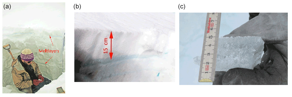
Figure 1 (a) View into the snowpit dug just after the 2012 rain/melt event at NEEM. The resulting melt layers occur in depths of around 15 and 70 cm below the surface. (b) Close-up of the upper melt layer and (c) close-up of the 3.5 cm thick layer.

A problem with interpreting melt layers is shown by the snowpit sampling performed during the 2012 CE melt event at NEEM (Figs. 1 and A1c). When a melt event creates multiple melt layers, the uppermost melt layers remain in the snow of that year and the lower ones may percolate into snow from previous years. This is also true for melt events that only form one layer, yet larger melt events seem to percolate deeper into the snowpack.

In the Appendix, we also present the result from a simple rain/melt event experiment performed in April 1995, using cold coffee as a colored substitute for melt (Fig. A1a, b). In a more recent study, Pfeffer and Humphrey (1998) perform a very detailed analysis of melt water infiltration into the snowpack. Therefore, interpretations of melt events on an annual timescale should be handled with care, and the uppermost layer should be taken as a reference. This effect can be neglected at decadal and lower temporal resolution.

1.4 Climate of the Holocene

Melt layers can be found in ice cores throughout the Holocene in central Greenland. To analyze and understand these, a climatic overview is necessary. Axford et al. (2021) have compiled different records of the Holocene climate in Greenland (Fig. 2), including the GISP2 melt layer record (Alley and Anandakrishnan, 1995). Their study offers two possible climatic reconstructions: a climatic optimum around the Early Holocene, as shown by pollen, geological records, and δ¹⁵N from ice cores (e.g., Fig. 2c), or a damped climatic optimum, as shown by the δ¹⁸O from ice cores (Fig. 2d). Based on ice core reconstructions, the dampening of these warm temperatures during the Early Holocene is due to a larger ice sheet with higher surface elevation (Fig. 2a, h) and therefore cooler temperatures due to a higher lapse rate (e.g., Brunt, 1933; Gardner et al., 2009; Vinther et al., 2009).

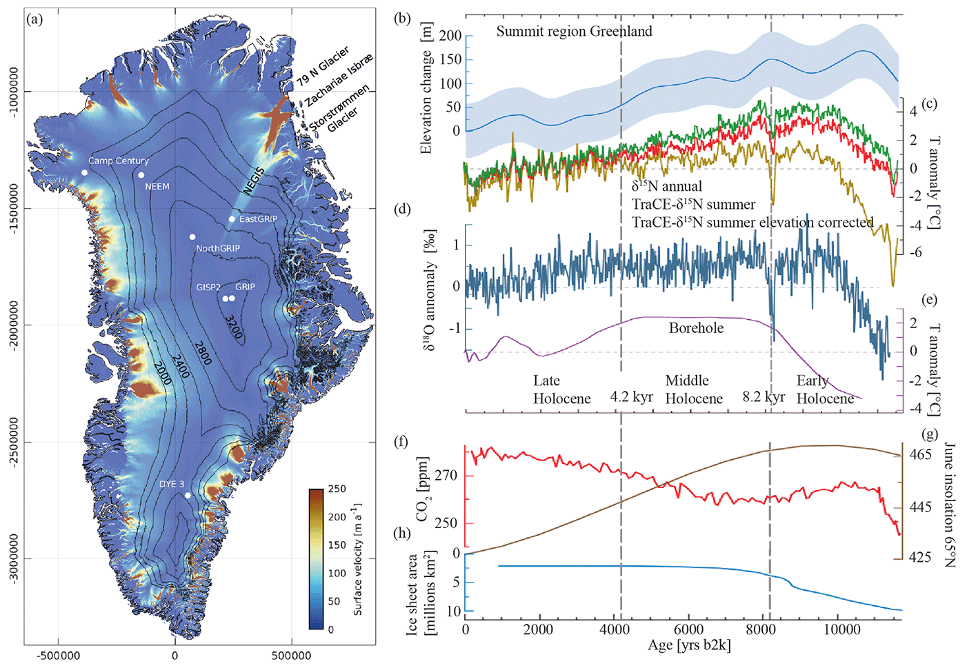
Figure 2 (a) Overview map of Greenland, including relevant ice core drill sites and surface velocities from Gerber et al. (2021). (b) Estimated surface elevation change at Summit (dark blue, Vinther et al., 2009) and uncertainty (faded blue shading, Lecavalier et al., 2013). (c) Annual δ¹⁵N (dark yellow) and summer (red) and elevation-corrected summer (green) Summit temperature anomalies from TraCE-δ¹⁵N (Buizert et al., 2018). (d) GRIP oxygen isotopes (Rasmussen et al., 2006; Vinther et al., 2006). (e) GRIP borehole temperature reconstruction (Dahl-Jensen et al., 1998). (f) Atmospheric CO₂ (Monnin et al., 2004). (g) Climate forcings and influences, including June insolation (Berger and Loutre, 1991). (h) Decline of the Laurentide–Innuitian–Cordilleran ice sheet complex (Dalton et al., 2020); note the reversed y axis. Panels (b–h) are modified from Axford et al. (2021, Figs. 2 and 3e); the vertical dashed lines mark the boundary between the Early and Middle and the Middle and Late Holocene at 8.2 and 4.2 ka, respectively, and all proxies are shown as anomalies relative to the 1930–1970 mean.

The timing and intensity of the Holocene Climatic Optimum (HCO) is still debated: e.g., Lecavalier et al. (2017) find an early and intense HCO, while, e.g., Badgeley et al. (2020) argue for a later HCO. Bova et al. (2021) argue that the warm temperatures at the beginning of the Holocene are a bias caused by proxies being mostly affected by warmer summer temperatures (Fig. 2g) and by larger seasonal variations, while the annual mean temperature remained lower and gradually climbed to today's value, more or less following atmospheric CO₂ concentrations (Fig. 2f).

1.5 The EastGRIP site

The East Greenland Ice Core Project (EastGRIP) ice core, based on which we create our melt layer record, is drilled through the Northeast Greenland Ice Stream (NEGIS, Fig. 2a). This ice stream flows from the ice divide, between NorthGRIP and the summit area, towards the NNE until it terminates at the coast (Vallelonga et al., 2014). The position of the EastGRIP drill site currently moves at approximately 55 m yr⁻¹ (Hvidberg et al., 2020), i.e., approximately 15 cm d⁻¹.

2 Methods

2.1 Depth of interest

Our analysis covers the upper 1090 m of the EastGRIP ice core, corresponding to the years 1965 CE to 7604 BCE, i.e., 9569 years. We use the age scale provided by Mojtabavi et al. (2020) and the time reference “years before the year 2000 CE” (years b2k).

The depth notation in this work refers to the depth below the 2017 ice sheet surface, the year in which ice core drilling began. Ice core processing started 13.75 m below the surface, which corresponds to the year 1965 CE (44 years b2k, Mojtabavi et al., 2020). Thus, this is the youngest material available for our analysis.

We terminate our investigation of bubble-free layers at a depth of 1090 m (approximately 9604 years b2k) because of the almost complete transition from air bubbles to clathrates (e.g., Shoji and Langway, 1987; Kipfstuhl et al., 2001; Uchida et al., 2014). With bubbles becoming smaller and eventually transforming to clathrates under increasing pressure, the spacing between bubbles increases and bubble-free layers become increasingly difficult to identify. This bubble–clathrate transformation is not a gradual process over depth, but has variable rates for different layers due to their physical properties and the resulting complex crystallization of air hydrates (Weikusat et al., 2015). Using the line scan images (next section), we find that the conversion from bubbles to clathrates is fully completed in a depth of 1150 m, but we end our analysis 60 m above that depth.

2.2 The line scanner and its images

The line scanner is a well-established and powerful tool for high-resolution analysis of ice stratigraphy, making use of contrast enhancement by the optical dark-field method (Faria et al., 2018). Different devices with similar setups have been used on many deep ice cores since the NorthGRIP drilling in 1995 (e.g., Svensson et al., 2005; McGwire et al., 2008; Jansen et al., 2016; Faria et al., 2018; Morcillo et al., 2020; Westhoff et al., 2020). The device used at EastGRIP is the second-generation Alfred Wegener Institute (AWI) line scanner. Images are obtained with a camera moving along the top of a 165 cm long and 3.6 cm thick ice core slab (Weikusat et al., 2020). Two light sources illuminate the polished ice core slab at an angle from below (for more details, consult Svensson et al., 2005 and Westhoff et al., 2020).

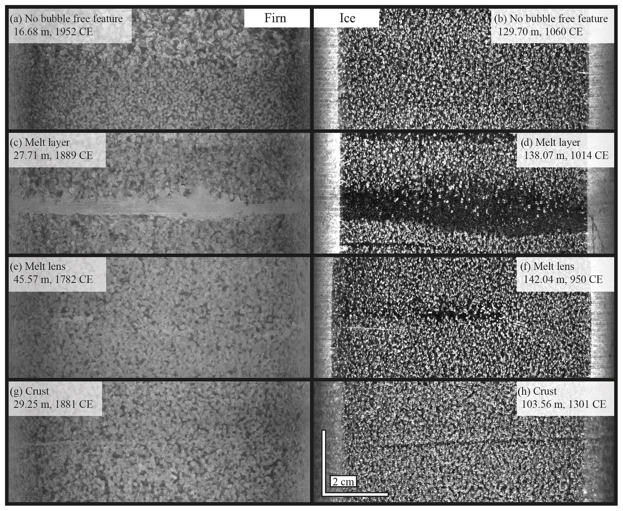
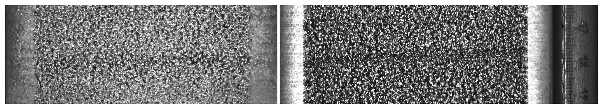
Figure 3 The appearance of different structures in line scan images of firn (left) and ice (right). (a, b) Typical examples of the appearance of firn and ice. (c, d) Bubble-free layers interpreted as melt layers. These are continuous horizontally across the ice core. (e, f) Bubble-free lenses interpreted as melt lenses, which are discontinuous patches that mostly have a horizontal elongation. (g, h) Very thin and straight bubble-free layers with sharp edges. These structures are hard to see in line scan images and are interpreted as crusts, the result of surface hardening by the wind.

The line scan images for firn and ice differ substantially (Fig. 3 left and right, respectively). In firn and snow, the bright sections of the image represent the solid parts, such as snow crystals, firn grains, or ice layers. The high number of firn grains, and thus many grain boundaries, reflect the light, causing the bright appearance. Dark sections of the image represent voids, i.e., air. When firn has been compressed to ice, the appearance of features is inverted: ice now appears dark, and bubbles (i.e., air) are now represented by bright pixels. In ice, the open pores and voids between single grains have been closed, which allows light to travel through without any reflections; thus, a dark field below the ice core slab is imaged. Bubbles appear bright, as their rounded ice–air interface offers perfect conditions for light scattering in all directions.

At EastGRIP, the firn–ice transition is situated at around 70 m depth (e.g., Buizert et al., 2012), so the largest part of our investigation is conducted on ice with bubbles, where bubble-free layers are easy to identify (e.g., Fig. 3d).

2.3 Types of events

In the upper 1100 m of the EastGRIP ice core, the majority of the ice contains bubbles, and thus has the “normal” appearance of firn and ice (Fig. 3a, b). Firn and ice can be bubble free for two reasons: either snow melted and refroze close to the surface, creating a melt layer or lens, or surface hardening took place, e.g., by wind, which forms hard (wind) crusts. On this basis, we define three types of bubble-free features: melt layers (Fig. 3c, d), melt lenses (Fig. 3e, f), and crusts (Fig. 3g, h). Within our three categories, we denote the certainty of our labeling as either “certain” or “uncertain.” The process of data acquisition and depth registration can be found in the Appendix.

We define the different types as follows:

• Melt layers are, in general, continuous features ranging across the entire horizontal core width (10 cm). The melt layer thickness can vary within one layer, but we define that it should always be greater than 1 mm at its narrowest point (1 mm = 18.6 pixels). Melt layers can have sharp edges (Fig. 3c, bottom left) or smooth edges where bubbles are within the melt layer (Fig. 3d, top edge).

• Melt lenses have the same appearance as melt layers, yet are of smaller dimensions and are not continuous across the width of the core. The definition of layer and lens is therefore determined by the core diameter, which in the EastGRIP ice core is approximately 10 cm. Lenses can have a rounded shape, yet, in general, they show elongation along the horizontal. These disk-shaped structures point to a melt layer above and, in order not to overestimate the number of events, the lens itself should thus not be seen as a separate event (Sepp Kipfstuhl, personal communication, 2021​​​​​​​).

• Crusts are very thin (around 1 mm thick) bubble-free layers that are, in general, continuous from one side of the core to the other. They have a sharp border with the bubbles around them. These thin layers can be identified reasonably well and distinguished from melt layers in the upper 250 m. Yet, as the thinning of layers proceeds, it becomes no longer possible to distinguish them from the 2D line scan images. We therefore assume that, below 250 m, all layers with the appearance of crusts are actually thinned melt layers. Thinning is influential to such a degree that crusts eventually become no longer detectable using line scan images.

2.4 Core breaks and the brittle zone

Core breaks influence the counting of melt layers and lenses. Core breaks are fractures in the core, which mainly occur for two reasons: they are produced when breaking the ice core free at the bottom of the borehole (see Westhoff et al., 2020) or are due to fractures in the brittle-zone ice (Neff, 2014). It is found that:

• Drilling-related core breaks are usually approximately horizontal. During smooth drilling operations and with good ice quality, core breaks occur every few meters, depending on the length of the core barrel chamber implemented in the deployed drilling system.

• In the brittle zone, where the internal pressure of the trapped air bubbles is very high and exceeds the tensile strength of the ice core, the ice core samples will break up and sometimes even explode. This is an effect of pressure–temperature relaxation after core recovery at the surface. Core breaks in the brittle zone can have any orientation and thus tend to run diagonally across the core and line scan image.

During line scanning, light is introduced at an angle from below the core slab. As the core breaks usually have a rough break surface followed by a gap and another rough break surface, the light intensity will drop when crossing the void. This intensity loss casts shadows on either side of the core break. These shadows greatly depend on the geometry of the core break and can easily be mistaken for a bubble-free layer. A rare occasion (one of two in total) is shown by Fig. 4, where a melt layer is very close to a break. The core break is distinguishable from the melt layer because the core break casts a shadow on the edge of the core slab while the edge remains at a constant brightness in the presence of the melt layer (yellow boxes in Fig. 4). Similar to the core break shadows are the saw-cut shadows, which appear at the ends of each 165 cm-long line scan.

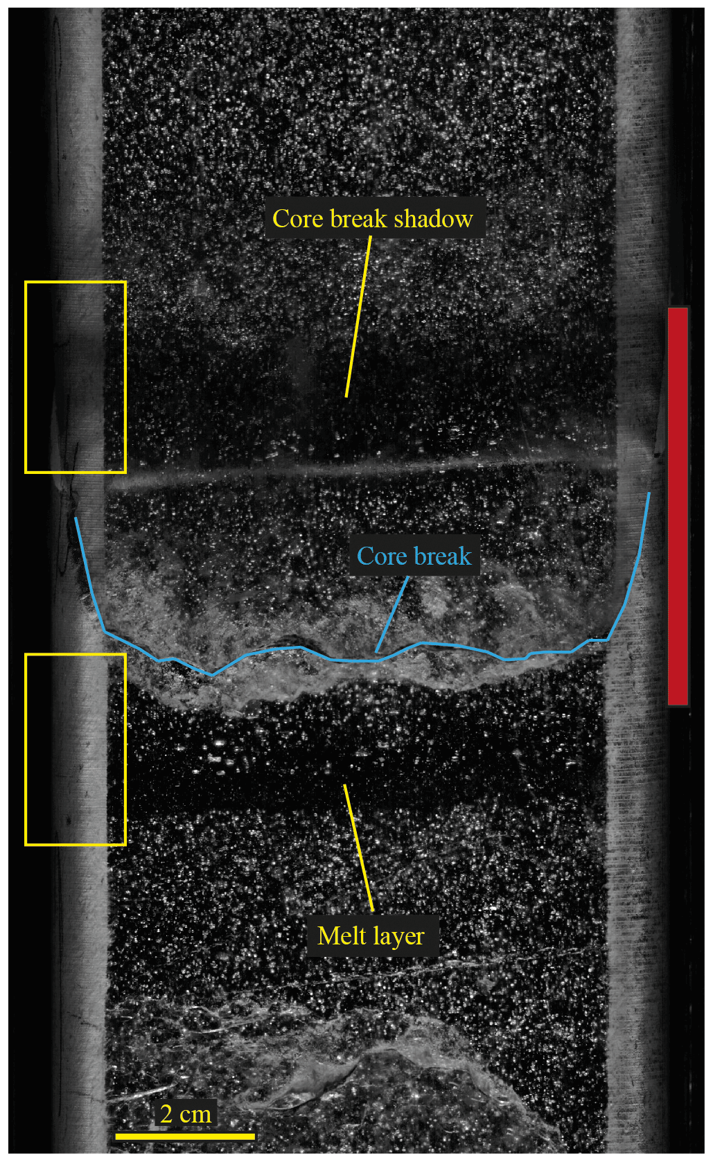
Figure 4 A core break casting a shadow and a melt layer have a very similar appearance in line scan images. A distinction is made based first on the proximity to the break and then on differences in brightness along the ice core's round drilling edge (yellow boxes). Core break shadows darken the edge of the sample. The minimum section not suited for analysis is indicated by the red bar.

To account for this difficulty, features close to core breaks and the edges of images are in general disregarded. This implies that the more core breaks we have, the more bubble-free events we may miss, and the more we underestimate the number of events. It is, therefore, necessary to obtain an overview of core breaks throughout the depth of interest. We estimate the chance of missing a bubble-free event by assuming a 4 cm sample loss for each break. In general, a shadow is cast 1.5 cm to either side of the break, and the break itself disturbs the image across at least 1 cm, adding up to 4 cm in total (Fig. 4, red bar).

2.5 Northern Hemisphere tree rings

Sigl et al. (2015) created a Northern Hemisphere temperature reconstruction using the tree ring composite record (N-Tree), which we compare to melt events. The tree ring record comprises tree ring growth anomalies from five different locations across the Northern Hemisphere, where temperature is the limiting factor on growth. The N-Tree record is presented based on its independent annual ring-width timescale (NS1-2011) and carries no uncertainty according to Sigl et al. (2015). The individual records from northern locations in Finland, Sweden, Siberia, Central Europe, and the USA almost always overlap, providing a composite average of the tree growth in response to temperature.

For the comparison of melt events to the tree ring data, we translate the EastGRIP (Greenland Ice Core Chronology 2005: GICC05) ages to the tree ring timescale (NS1-2011). We verified that there is good alignment of EastGRIP and N-Tree data, as many volcanic eruptions align with drastic cooling events to within 1 to 2 years. We refer to ages and events using the GICC05 timescale for consistency throughout the paper.

3 Results

3.1 Melt events

We find 561 melt events throughout the last 9700 years in the EastGRIP record (Fig. 5c), which can be separated into 137 melt layers (Fig. 5a) and 424 melt lenses (Fig. 5b). Melt lenses are thus almost 3 times more frequent and represent smaller events. We find another 622 uncertain events, of which 157 are uncertain melt layers and 465 are uncertain melt lenses (Fig. A2).

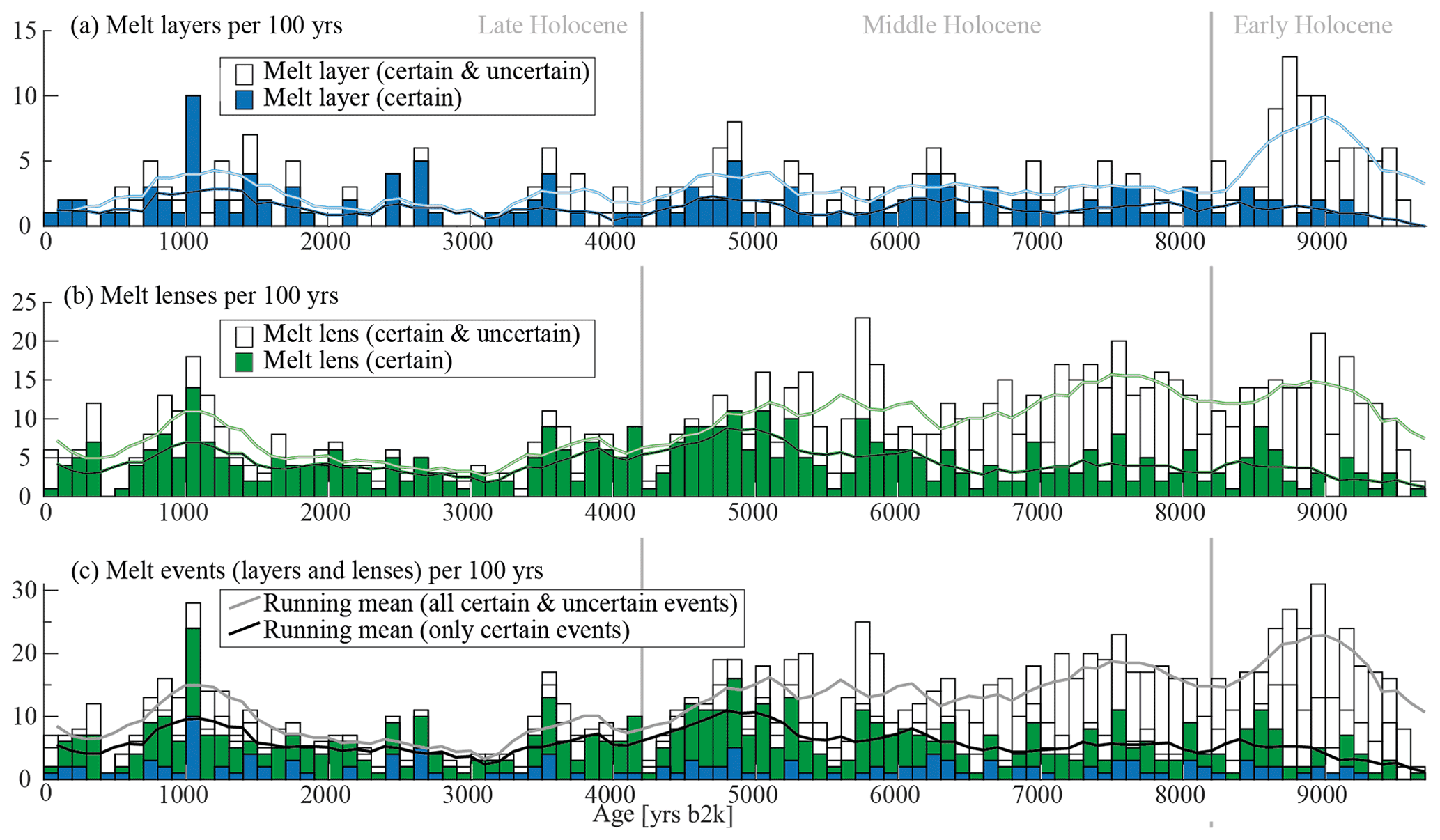
Figure 5 Number of melt layers and lenses per century throughout the last 9700 years in the EastGRIP ice core. Running means are shown as solid lines. (a) Melt layers (dark blue) and uncertain melt layers (white). (b) Melt lenses (dark green) and uncertain melt lenses (white). (c) Melt events, i.e., panels (a) and (b) stacked, including their uncertainties. Note that the bar representing the period from 0 to 100 years b2k represents only 56 years, not 100 years like the other bars, as our analysis begins in 1956 CE.

Both melt lenses and layers follow the same trend and are most abundant during the same periods. As both features represent refrozen melt water, we can consequently group them together as melt events (Fig. 5). For events we are certain of, we see a gradual decrease in the number of events towards the Early Holocene. We find very few or no melt layers around the years 500, 2000, and 3000 b2k, and melt lenses are also less frequent. We find many certain melt events (dark blue and dark green in Fig. 5) around the years 1000, 3500 to 4000, 4500 to 5200, and 6000 b2k. We then continuously find melt events in between 6000 and 9000 years b2k, but varying in number.

Including uncertain events, the number of events shows a slight increase towards the Early Holocene. These are melt layers and lenses that are difficult to see in the line scan data, and should thus be treated with caution.

Events older than 9000 years become difficult to detect due to progressive bubble to clathrate transformation; therefore, values gradually decrease. Slightly before 9000 years b2k, the ratio of uncertain to certain layers increases, indicating the difficulty of detecting melt layers. Also, we do not capture the most recent years, i.e., those younger than 44 years b2k (1956 CE).

3.2 Core breaks and their implications

We count core breaks (Fig. 6a, orange bars) in the upper 1100 m of the EastGRIP ice core and show the corresponding ages and depths. The running mean over 16.5 m (Fig. 6a, brown line) clearly locates the brittle zone as lying between 650 and 950 m depth. In the brittle zone, the number of core breaks greatly increases and exceeds three breaks per meter (or five breaks per 165 cm sample). As a core break masks 4 cm, we lose almost 25 % of the sample in sections with six core breaks per meter.

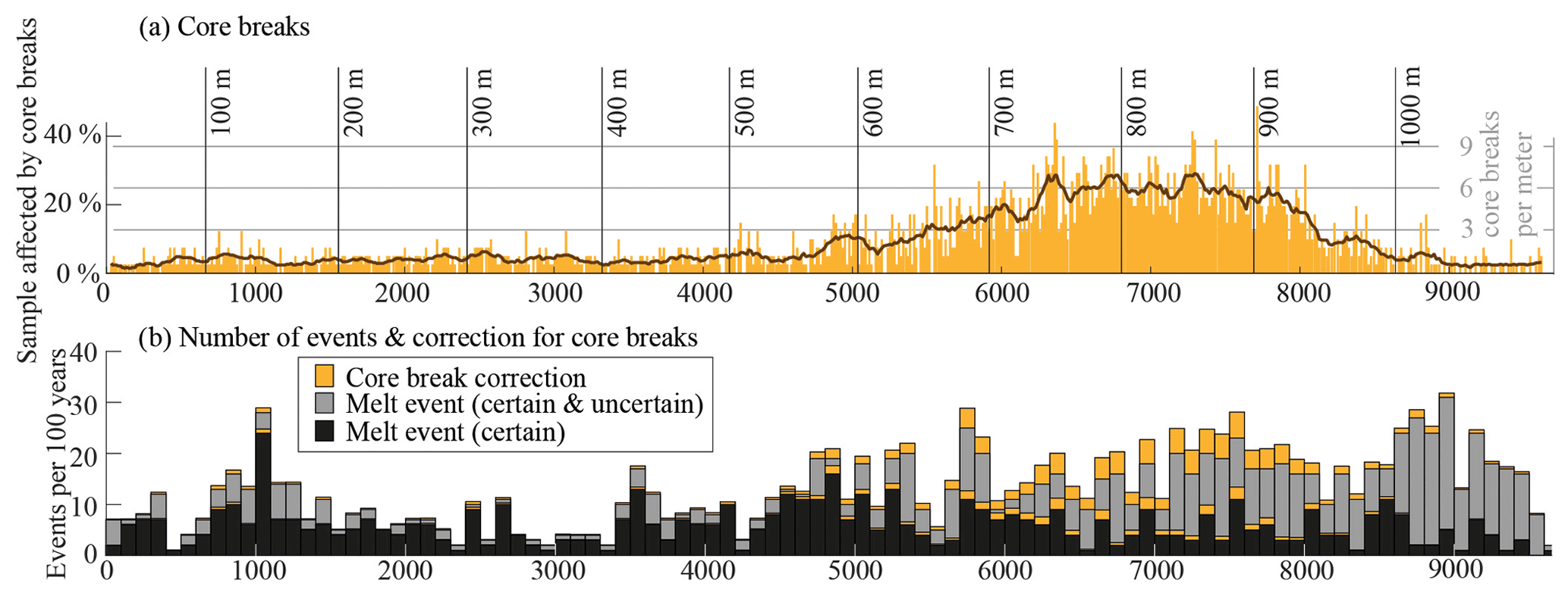
Figure 6 (a) Percentage of a 165 cm sample affected by core breaks (orange bars, scale on the left side), number of core breaks per meter (orange bars, scale on the right side), and running mean over 16.5 m (brown line). The broad peak between 650 and 950 m depth indicates the brittle zone. (b) Certain melt events (black) and uncertain melt events (gray) corrected for potentially missed events in the proximity of core breaks (orange).

As we know the number of melt events per sample, we can estimate the number of events missed due to core break shadows (Fig. 4). Events per 100 years are shown by vertical bars, and the potentially missed melt events, i.e., our core break correction, are shown in orange (Fig. 6b). The largest corrections are therefore performed in the brittle zone, where we add around 25 % to the number of melt events. This does not change the overall picture much, but it shows that we probably underestimate melt events in the time between 6000 and 8000 years b2k.

Our correction described above assumes no correlation between the locations of core breaks and melt layers. This correlation could be expected, as melt layers might affect the crystal structure or other physical properties of the core. We performed a nonquantitative visual inspection and did not find any connection of melt layers to weakening or strengthening of the ice, which would affect the initiation and location of core breaks in the brittle zone.

3.3 Melt layer thickness and total melt

We have documented the thicknesses of the 137 certain melt layers (M₀, Fig. 7). Melt lenses are excluded from this analysis, as their average thickness is below 1 mm and has not been measured. The layer thicknesses of melt layers are shown by the yellow, orange, and red bars; to distinguish events occurring within a short period, the layer thicknesses are indicated by circles. Cases of multiple events within 5 years are marked with a star (Fig. 7c). We find three cases with three or more events within 5 years (red stars) and 13 cases with two layers in 5 years (blue stars).

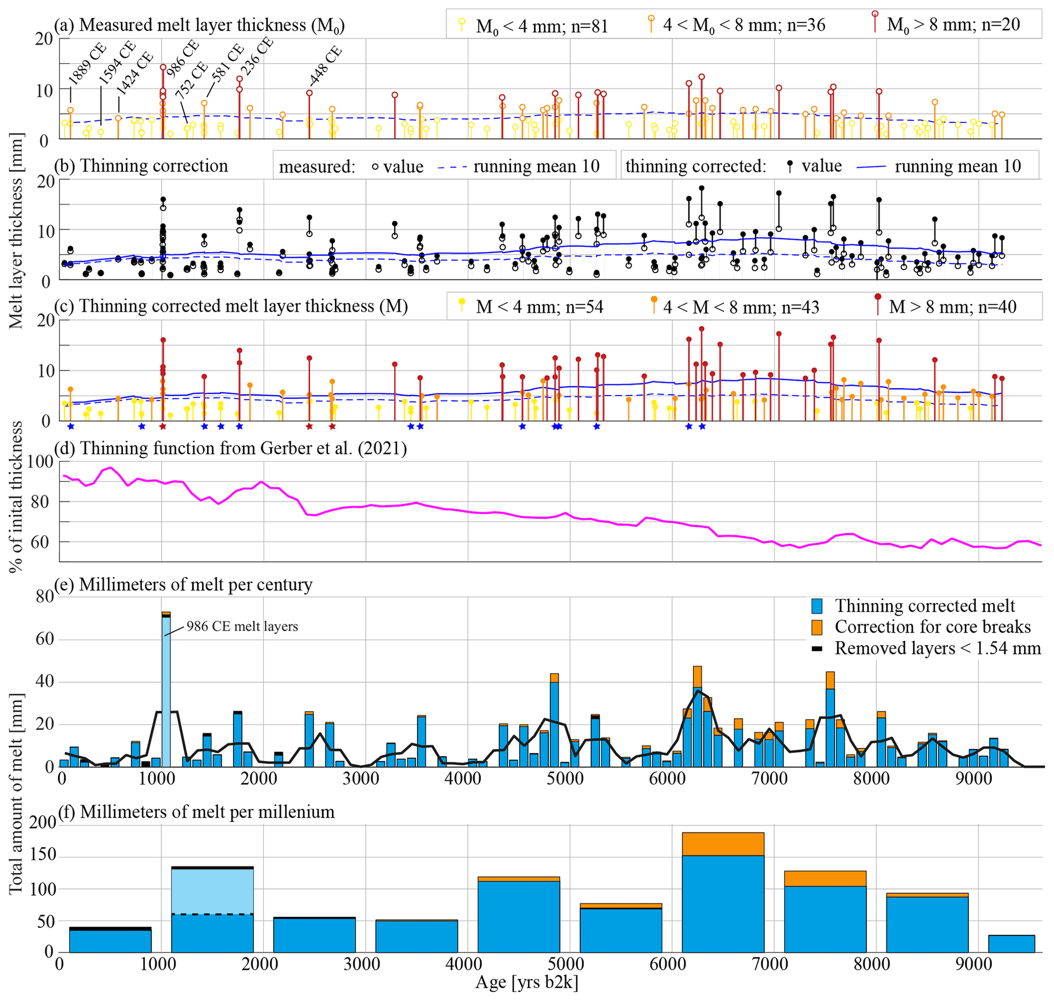
Figure 7 The layer thicknesses of melt layers are shown by the yellow, orange, and red bars (smaller than 4 mm, between 4 and 8 mm, and greater than 8 mm, respectively). To distinguish events occurring within a short period, the layer thicknesses are indicated by circles (measured thicknesses M₀ are indicated by open circles, and thinning-corrected thicknesses M are indicated by closed circles). Running means of 10 events are indicated by dashed (for measured thicknesses) and solid (for thinning-corrected thicknesses) blue lines. Panel (a) shows events that were later compared to tree rings, along with their dates in CE notation. (b) Individual layer thicknesses corrected for thinning using the thinning function from Gerber et al. (2021) shown in (d). Stars in (c) mark multiple events within 5-year periods (blue stars indicate two events, red stars indicate three or more). Panels (e) and (f) show the millimeters of melt (blue bars, calculated from melt layer thicknesses) per century (e) and millennium (f), potentially missed events due to core breaks (orange), removed layers smaller than 1.54 mm (black, see Fig. A4), and the running mean (black line). Melt layers around the year 986 CE are plotted in light blue.

We correct the melt layer thickness for thinning, i.e., we correct the initial thickness M₀ (shown as open circles in Fig. 7a, b, c) to the corrected thickness M (shown as filled circles), using the thinning function from Gerber et al. (2021, Fig. 7d). Here, we must keep in mind that the thinning is an average over tens of meters derived from radar data. It is thus an upper limit assumption for the thinning of melt layers, which are denser (due to the lack of bubbles) and should therefore thin less than the surrounding ice.

Thin melt layers (M<4 mm, yellow) are found throughout the Holocene, yet they seem to be more abundant in the Late Holocene (the last 4200 years). Thick melt layers (M>8 mm, red) become more frequent further back in time (positive blue trend line in Fig. 7b). The thinning-corrected running mean (solid blue line in Fig. 7b, c) points to an average melt layer thickness of around 5 mm for the past 4500 years. Going back further in time, we see a gradual increase in melt layer thickness in ice older than 4500 years (Fig. 7c), peaking at an average thickness of 8 mm around 6500 to 7000 years b2k (solid blue line). In events older than 7000 years, the mean gradually drops. We find that the last melt layer in the ice was deposited 9235 years b2k.

We expect to miss thinner melt layers the further back we go in time, which is seen in our results (Fig. 7c), as we find only seven thin melt layers (M<4 mm, yellow) between 7000 and 9700 years b2k. In the same period, we find 15 medium (4 mm $<M<$ 8 mm, orange) and nine thick (M>8 mm, red) melt layers. Assuming we miss thin layers but not thicker ones, we would expect a continuous increase in average melt layer thickness. Yet this average (blue line in Fig. 7c) gradually drops below 7500 years as we approach the Holocene Climatic Optimum (HCO). A possible reason for this gradual drop could be the two cooling events 8200 and 9300 years ago (Alley et al., 1997; Thomas et al., 2007; Rasmussen et al., 2007).

We only find melt layers exceeding a thickness of 15 mm between 6100 and 8100 years b2k, with one exception at 1014 years b2k (Fig. 7c). This allocates the majority of the thick melt layers to the Middle Holocene (Northgrippian period; Cohen et al., 2016). An overview of the thickness distributions can be found in Fig. A3.

Derived from melt layer thicknesses, we present a melt layer record of the total amount of melt per century and millennium (Fig. 7e and f, respectively). This record is corrected for thinning using values from Fig. 7c, and we account for potentially missed layers due to core breaks (orange, from Fig. 6). Layers thinner than 1.54 mm have been removed for consistency (see Fig. A4).

Millimeters of melt per century (Fig. 7e) shows the high variability of melt events, as some centuries do not contain any events. Yet, the running mean (black line) shows distinct spikes around 4500 to 5000, 6000 to 6500, and 7500 years b2k. These coincide with the period of the HCO. The HCO is also apparent in the amount of melt per millennium (Fig. 7f), with a peak in the interval between 6000 and 7000 years b2k.

In both plots (centuries and millennia), there is a particularly prominent peak at around 1000 years b2k (light blue). The melt event from this period, i.e., 1014 years b2k or 986 CE, was of such an intensity that it left an unprecedented spike in the melt record of the past 10 000 years. Here, it is important to note that this is an event confined to a short period of one or a few summers, and not a signal that is representative of the entire century or millennium.

4 Discussion

4.1 Integrity of our (and other) melt layer records

If a melt lens is behind bubbles, it becomes hard to see in our 2D images, and will probably be classified as uncertain or missed completely (Fig. A2). The prominent and big events will not be missed with our analysis as they are very obvious in line scan images. To further reduce the likelihood of missing events, our analysis was done twice, minimizing operator errors.

We may also miss bubble-free layers in the ice sheet's stratigraphy due to the ice core's restricted diameter. Studies such as Keegan et al. (2014), Schaller (2018), Fegyveresi et al. (2018), Taranczewski et al. (2019), or our coffee experiment (Fig. A1) show the high spatial variability of melt lenses in trenches or shallow cores. While the spatial distribution of a melt lens or a layer is not homogeneous over larger areas, our ice core with a diameter of 10 cm is a very narrow sample of the ice column. Keegan et al. (2014) show that big melt events such as the 1889 CE event are visible in most shallow cores and snowpits, thus proving they have a widespread distribution. For bigger events, we can therefore assume that our analysis is representative of the largest part of northern Greenland, while smaller events might be restricted to local areas.

4.2 The highly dynamic EastGRIP site

The EastGRIP ice core is drilled into the NEGIS (Fig. 2a) with a surface velocity of 55 m yr⁻¹. Gerber et al. (2021) track the location of ice from EastGRIP back over time and show that, e.g., 9000-year-old ice was deposited 170 (±17) km further southwest and at a 270 m higher elevation. For their calculations, Gerber et al. (2021) use today's ice sheet dimensions, but, as Vinther et al. (2009) show, the ice sheet elevation has not been constant over the Holocene (Fig. 2b). NEGIS originates from an area somewhere between the NorthGRIP and GRIP sites. Vinther et al. (2009) suggest that these two sites were at an elevation that was 150 to 200 m higher at the beginning of the Holocene, than they are today.

Adding the values from Vinther et al. (2009) and Gerber et al. (2021), the true elevation change over the past 9000 years could lie around 400 m. Using the lapse rate estimate of temperatures decreasing by 0.6 to 0.9 ^∘C every 100 m of elevation gain (Gardner et al., 2009), we can deduce a temperature change at the EastGRIP drill site of 2.4 to 3.6 ^∘C (or 3 ± 0.6 ^∘C) based on the 9000 years that have elapsed and on it flowing downstream, without considering any climatic changes. Thus, when analyzing EastGRIP ice, we must take into account the spatial variations with time.

Alley and Anandakrishnan (1995) suggest that an increase of 2 ^∘C causes a 7.5-fold increase in melt frequency, based on a comparison of their GISP2 melt layer frequencies to a record from site A (Alley and Koci, 1988). Assuming this linear relationship between melt layers and temperature to be correct, we would expect a more than 10-fold increase in melt frequency for EastGRIP from the Early Holocene to today, solely due to the lowering of the site elevation. An increase in frequency of such a magnitude is not supported by our data. On the contrary, the amount of melt and the average thickness of a melt layer decreases from the Early Holocene to today (see Fig. 7f). Thus, cooling or decreasing summer insolation outweighs the warming from the elevation drop. Despite the lower surface elevation today and the corresponding 3 ± 0.6 ^∘C warming, our data suggest that melt events around the HCO were more intense (Fig. 7) and more frequent (Fig. A5).

4.3 The EastGRIP melt layer record

In comparison with ice core melt layer records from southwestern Greenland (Trusel et al., 2018), Renland, coastal Greenland (Taranczewski et al., 2019), or northern Canada (Fisher et al., 2012), the record of 831 mm melt in 10 000 years of the EastGRIP ice core is rather low. However, we must keep in mind that the average summer temperature at EastGRIP is around −25 ^∘C, making melt events a rare phenomenon. It is therefore almost surprising that we find 137 melt layers and 424 melt lenses at a site with such cold summers.

4.4 The melt layers of the 986 CE event

When analyzing melt layers on an annual timescale, the well-studied 2012 CE melt event in Greenland (e.g., Nghiem et al., 2012; Bonne et al., 2015; Nilsson et al., 2015) helps our understanding of natural melt events. The infiltration of melt layers from different years into the stratigraphy could potentially ruin the consistency of, e.g., isotope records that assume the stratigraphy to be linear in time. This certainly adds another factor of complication to the temporospatial variability recently observed and discussed (e.g., Steen-Larsen et al., 2011; Münch and Laepple, 2018). In hindsight, it is not possible to distinguish between two scenarios: (1) 5 consecutive years with surface melting each summer, which then creates a melt layer in each of the corresponding snow layers, or (2) one large melt and rain event that creates melt layers scattered across all the snow from the last 5 years below. For smaller events, the first option seems likely. For larger events, creating thick melt layers, the chances are high that melt percolates deep into the wet and warm snowpack, disrupting the stratigraphic order.

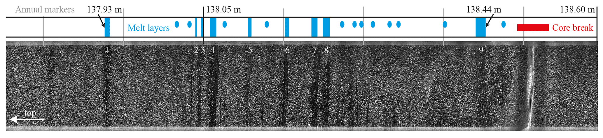
Figure 8 Nine melt layers and 12 melt lenses (blue bars and ellipses, respectively) within just 50 cm at around 138 m depth. Vertical gray lines represent annual markers. The depth 138.05 m corresponds to the year 986 CE (GICC05) or 991 CE (GICC21).

At a depth of around 138 m, we find 9 melt layers and 12 melt lenses within just 50 cm (Fig. 8). This depth interval represents the years 988 to 982 CE (on the GICC05 timescale). Adjusting to the new GICC21 timescale (Sinnl et al., 2021), this corresponds to the years 993 to 987 CE.

According to the thinning function of Gerber et al. (2021), at this depth, the layers have been thinned to approximately 90 % of their initial thicknesses (Fig. 7d). The thinning function works reliably in firn and ice, yet the melt layers must have been formed while the snow was still loosely packed on the surface. With today's accumulation rate, the upper 1.5 m of the snowpack contain 5 years of snowfall (Kjær et al., 2021).

The nine melt layers might not represent nine separate events; they could have been created in one single event. It may be possible that melt water percolated approximately 1.5 m deep into the snowpack and left nine melt layers. All of these layers would thus may have formed within a few days. During the 2012 CE warm event, with rain, melt percolated 0.7 m into the snowpack at NEEM, i.e., half the depth of our event (Fig. A1c). This leaves two assumptions: (1) the 986 CE event was more intense than the 2012 CE event, or (2) we are looking at multiple summers with surface melt. As shown in Fig. 8, layer 1 (137.93 m) is located 1 year above layer 2, while layer 9 is located 2 years below layer 8. The close proximity of layers 2 and 8 hints at a single formation event, similar to the 2012 CE event (Fig. A1). It could thus be that three consecutive warm summers created this melt layer sequence.

Assuming the melt layers around 986 CE to have formed in one event, then this must have been a long-lasting period of high temperatures and/or of intense rainfall. Rain events are rare on the Greenland ice sheet, and melt events such as the 2012 CE event are clearly noticeable, given the many melt layer traces they leave. It is also worth noting that the 1889 CE melt event, which is present in most areas and ice cores across Greenland and therefore considered a big event, consists of only two melt layers with a total of 8.5 mm melt. The 1889 CE event must therefore not have been as intense as the 986 CE (total of 63.2 mm melt) or the 2012 CE event. The only melt event comparable to the 986 CE event – although with significantly thinner layers – happened around the year 675 BCE (2675 years b2k and 328 m depth, Fig. 7c), with four melt layers and three melt lenses occurring within the stratigraphy of 1 year, and a total of 11.7 mm melt. Thus, events with many melt layers are rare in Greenland, even over the course of the entire Holocene.

In a previous version of this work, we noted a possible connection between the 986 CE event and the settlement voyages of Erik the Red from Iceland to Greenland in the same year. Applying the GICC21 timescale (Sinnl et al., 2021), and considering the melt layers (Fig. 8) to be three events, then they would have occurred in the years 993, 991, and 988 CE. This would date them to a few years after the Vikings reached Greenland, and the events could have provided the Nordic settlers with warm summers in their first years on Greenland. Nevertheless, the 986 CE melt layer marks the beginning of consecutive warm periods, which are also preserved in tree ring data (see the next section).

4.5 Melt layers and Northern Hemisphere tree rings

We use the tree ring data (Sigl et al., 2015) to compare to melt layers. For seven melt events (see Fig. 7a), we evaluate the age offset of the melt event from the highest peak in the tree ring record (Fig. 9a) within an ±6-year window around the melt event (Fig. 9b–h). Each melt event lies very close to a tree ring peak; in most cases within the same year. Two events show an offset of 4 to 5 years from the highest peak within the ±6-year window (E4 and E6, Fig. 9e and g, respectively). We find a slightly smaller peak around the same year as the melt layer. Thus, we attribute this offset to incorrect peak assignment. All highlighted events (black boxes, E1 to E7) have at least one tree ring peak (warm anomaly) in very close proximity. For the 986 CE event (E3, Fig. 9d), the most prominent melt event in our record, we find a tree-ring warm year that is about 2.4 years older.

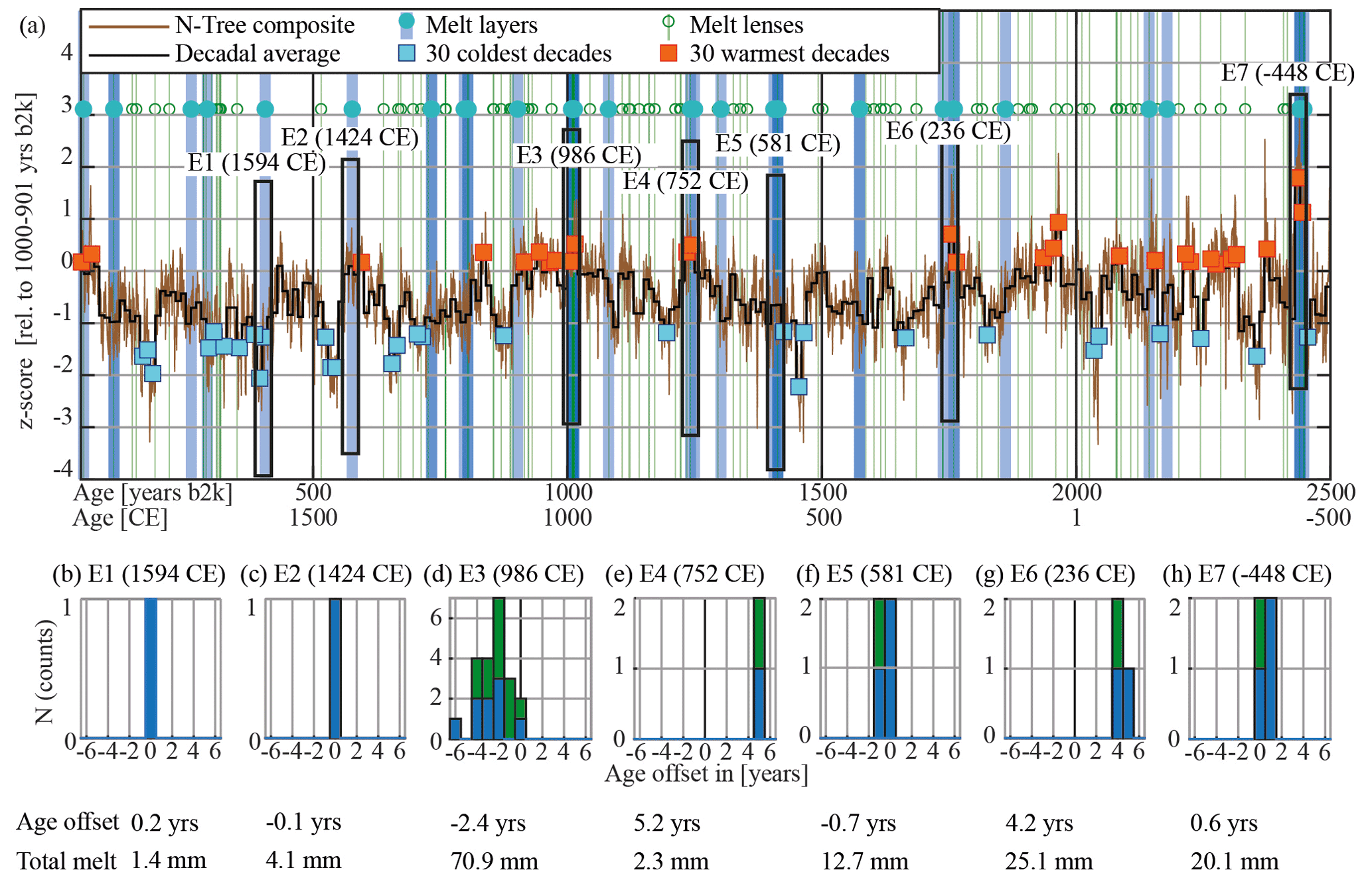
Figure 9 Tree-ring growth anomaly (Sigl et al., 2015) compared to the EastGRIP melt record from 44 to 2500 years b2k. (a) The tree-ring growth anomaly (brown) is averaged to decadal resolution (black), and the 30 warmest and 30 coldest decades are marked as orange and light blue boxes, respectively. Vertical bars highlight melt layers (blue) and lenses (green) at the corresponding ages. Seven melt events (E1 to E7) are highlighted by black boxes. (b–h) Histograms of the age offset of a melt event from the largest tree-ring growth year within ±6 years (layers in blue, lenses in green). The exceptional 986 CE event (E3) is younger than the tree ring maximum by about 2.4 years. The entire figure is based on the NS1-2011 tree ring timescale; the only exceptions are dates of events, e.g., 986 CE, which are based on GICC05 for consistency.

A more recent, 2000-year, temperature reconstruction from Büntgen et al. (2020) shows a distinct tree ring peak in the year 990 CE, coinciding with our E3 event, which spans across the year 990 CE on the the GICC21 timescale (Sinnl et al., 2021). The shifts of some of the other tree ring peaks by a few years from the compilation of Sigl et al. (2015) to Büntgen et al. (2020) still leave our melt layers in close proximity to these peaks.

The melting at EastGRIP might not be synchronous with all tree ring peaks, but it still offers some insight into the correlation of melt and tree ring growth on a larger geographic scale. This is also the case for volcanic eruptions: many volcanic events do not correspond to deep cooling in the tree ring records, although local minima are often observed in correspondence. Due to the age uncertainty of melt events and difficulties in timescale translations, we cannot evaluate a more precise age offset. Moreover, even though more melting occurs during tree-ring warm decades, not every prominent peak in the tree ring record has melt events in its proximity.

The location of EastGRIP might not represent the complexity of the climatic dynamics that produces tree-ring growth anomalies at scattered locations around the Northern Hemisphere, but the occurrence of more melt in warm periods and in proximity to some of the warmest years suggests a partial correlation. We expect that future studies could improve the results we have presented, in particular for the correlation of the melt events at EastGRIP with other ice cores and with more temperature records from the Northern Hemisphere.

5 Conclusion

We have created a melt record from the EastGRIP ice core covering the largest part of the Holocene. This record is only the second one, after Alley and Anandakrishnan (1995), that covers central Greenland. In the Early and the beginning of the Middle Holocene, we find the thickest melt layers (Fig. 7c), and also more melt per century or millennium than in the younger part of the Holocene (Fig. 7e, f). Nevertheless, the most occurrences of melt layers within a few years are found in the Late Holocene (Fig. 7c), e.g., the 2012 CE, 986 CE, and 675 BCE events.

The melt event that left the most melt layers in our record was the 986 CE event, followed by the 675 BCE event. The 2012 CE event is not displayed in our record but seems to have left similar traces to the 986 CE event (Fig. A1). So far, the 986 and 2012 CE melt events are unprecedented in the Holocene. This extends the statement of Trusel et al. (2018), who find the 2012 CE event to be unprecedented in the most recent 350 years. Although the 2012 CE melt, and rain, event is considered an exception, it could be a hint as to what we can expect for future summers in Greenland as global warming proceeds.

In our melt event record, we distinguish between melt layers and lenses and compare the most recent 2500 years to the tree ring temperature anomaly record from Sigl et al. (2015). We find that some peaks in the melt events and the tree ring data align (with an offset of a few years, see above). The large melt events stand out in the tree ring record from Sigl et al. (2015, Fig. 9) and also in the record of Büntgen et al. (2020, not compared in detail here). Warm events found in ice cores and tree rings therefore hint that outstandingly warm summers are a phenomenon over the entire Northern Hemisphere. While this is not strictly in agreement with our understanding of atmospheric circulations (e.g., Bonne et al., 2015; Hanna et al., 2016; Graeter et al., 2018), the effect could also be restricted to some trees used in the tree ring composite, introducing a warm bias for those particular years.

The value of a melt record from the EastGRIP ice stream ice core is due to its change of location and elevation over the past 9000 years. Today, the highly dynamic EastGRIP site is 170 km further north-northeast and 400 m lower than 9000 years ago. With a corresponding lapse rate of 0.6 to 0.9 ^∘C per 100 m, the temperature has increased by 3 ± 0.6 ^∘C over the past 9000 years. This temperature change is solely connected to the drop in elevation and not any climatic changes. Yet, this change has implications for the climate, as we find more and thicker melt layers in the Early Holocene than today (Fig. 7), whereas an increase in temperature of over 3 ± 0.6 ^∘C would suggest that there should be more and thicker melt layers today. This implies that the local warming caused by the elevation drop does not compensate for the summer temperature cooling over the Holocene. Our data therefore strongly suggest that Greenland summer temperatures must have been more than 3 ± 0.6 ^∘C warmer during the Early Holocene than today. The full-year average temperature from the GRIP borehole temperature follows the same trend as our melt layer proxy for summer temperatures, suggesting a stable Middle Holocene temperature and a decrease, with fluctuations, over the Early Holocene.

Melt records from central Greenland deep ice cores, e.g., GISP2 or EastGRIP, are subjected to less horizontal thinning in the Early Holocene than shallower ice cores, e.g., the RECAP ice core (Alley and Anandakrishnan, 1995; Taranczewski et al., 2019). This has the advantage that the Early Holocene melt record is preserved to a higher resolution, and our melt layer record thus differs from the melt reconstruction from Taranczewski et al. (2019). Nevertheless, due to the bubble–clathrate transition at around 1100 m depth, our melt layer record ends approximately 9300 years before today, as does the record of Alley and Anandakrishnan (1995). Establishing melt layer records below this depth/age remains a challenge due to the lack of bubbles and therefore the inability to find bubble-free layers. One approach to this problem would be to analyze the bubble distribution in line scan images, and the first steps in this approach have been done by Morcillo et al. (2020).

Our melt layer record can provide the basis to better understand summer temperatures in the Holocene, as the melt layers pinpoint warm events. The frequency or temporal distribution of these events can be incorporated into climate reconstructions or modeling studies (e.g., McCrystall et al., 2021). Melt layer records are therefore valuable climate archives, preserving single warm events over the course of millennia.

Appendix A

A1 Real-time observations of the 2012 CE melt event

While ice core studies of melt events show the finished picture of melt layers, lenses, and pipes (see the “Methods” section) in the snowpack, the 2012 CE melt event at NEEM offered a unique chance to observe the creation of these structures in real time. The warm event in 2012 CE lasted from 12 to 15 July, with temperatures varying around 0 ^∘C (Bonne et al., 2015). On those days, snowpits revealed the appearance of ice layers at different depths over time (Fig. A1c). Depth is relative to the snow surface and, due to the warming of the snowpack, the whole surface level lowered about 10 to 15 cm over the course of the warm event. This explains the apparent “rise” of the uppermost ice level over time – the surface was actually lowering. To acquire undisturbed data, the trench was widened by approximately 0.5 m every measurement day. This widening slightly changed the depth registration of each ice layer, which shows the high spatial variability of ice and melt layers in the snowpack.

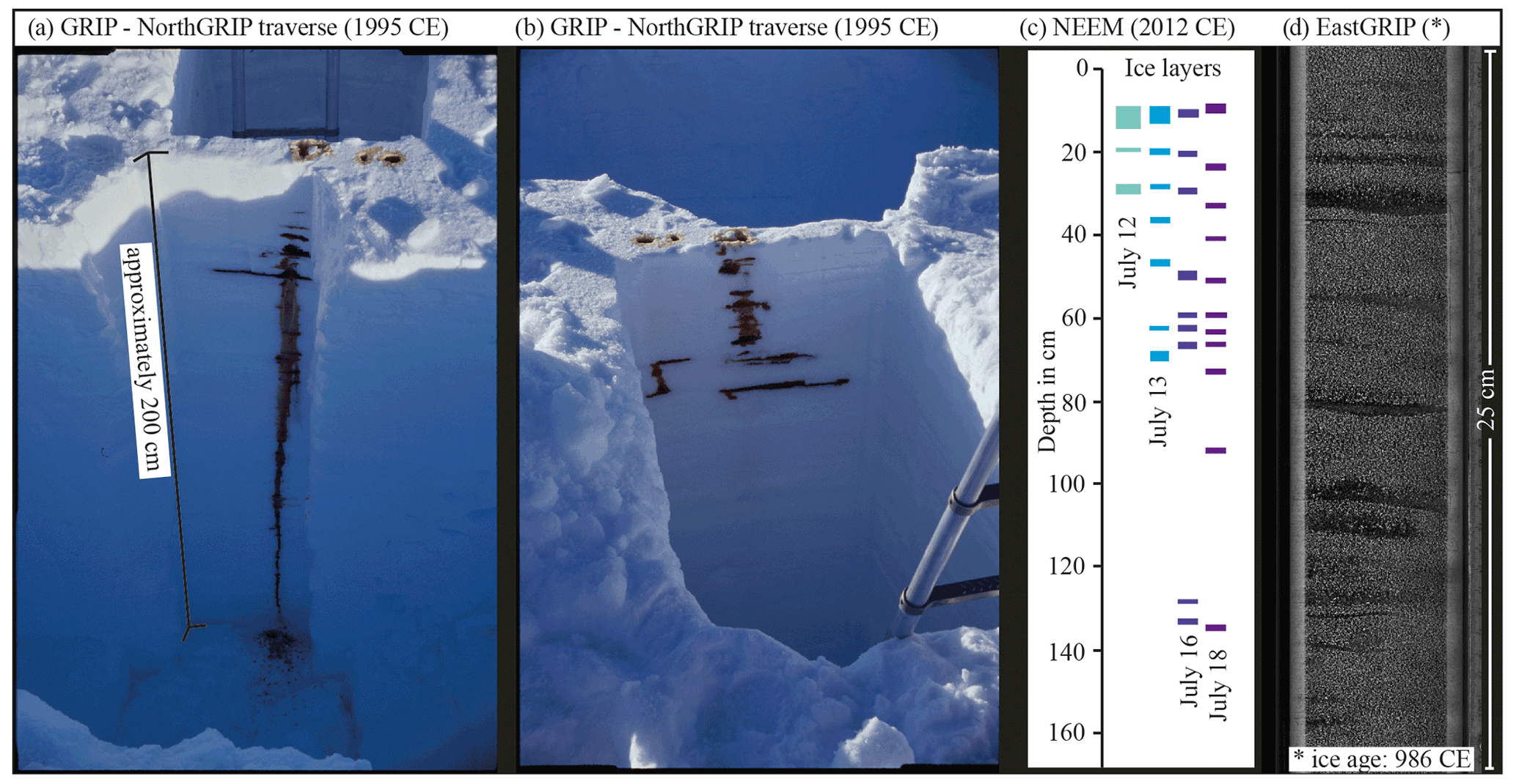
Figure A1 (a, b) Two sides of the same double trench, with three coffee injection points visible on the surface of the trench wall. Vertical coffee pipes are not always visible, but the horizontal coffee layers and lenses are very pronounced. The long vertical pipe reaching the bottom in (a) is due to the ex-filtration of coffee from the trench wall. The second trench, shown in (b), was dug after coffee injection. The trench's depth was approximately 2 m. (c) Appearance of ice layers at different depths during the warm event in 2012 CE at NEEM. Measurements were made by extending the same snow pit, which was revisited over the days of the warm event. (d) Upper half of a line scan of bag 252 (top at 138.05 m depth, years 986 to 989 CE) with multiple melt lenses and layers.

By 12 July, a substantial warming of the surface snowpack was observed, with the top 12 cm of the snowpack close to melting point (­0.2 ^∘C) and the development of more ice or refrozen melt layers at depths 22 and 32 cm. The surface snowpack had warmed considerably by 13 July, with further thickening of melt layers and the development of a 3.5 cm thick melt layer at 70 cm depth (Fig. 1c). Local rain contributed to this rapid warming of the top 65 cm of the snowpack to near-­melting temperatures. Somewhat cooler conditions on 14 July saw some cooling of the lower part of the snowpack. 15 July was the last day of warming observed in the snowpack, with the uppermost 80 cm of the snowpack near melting ­point, the warming of deeper snow down to 1.5 m depth, and the deeper percolation of melt water to 1.5 m depth. Observations from 16 July indicate a cooling of the snowpack from both above and below, with complete refreezing of the surface snow by 18 July.

Experimental simulations of melt events have been performed by Das and Alley (2005) and Humphrey et al. (2012), but in situ observations have only been conducted at NEEM (e.g., Bonne et al., 2015) and Summit in 2012 CE (e.g., Bennartz et al., 2013). Older melt events can be found in ice cores using visual methods (Fig. A1d), such as the line scanner (see the “Methods” section).

A2 The coffee experiment

We present the results from a simple rain/melt event experiment performed in April 1995 on a traverse from the Greenland Ice Core Project (GRIP) site to the Northern Greenland Ice Core Project (NorthGRIP) site in Greenland (Fig. A1a, b). Next to an existing trench (Fig. A1a), three shots of coffee were poured into the snow, simulating the infiltration of superficial water into the snowpack. A second trench was dug (Fig. A1b), leaving an approximately 30 cm thick wall between the two trenches. This is commonly done to visualize different structures in the snowpack (e.g., Fegyveresi et al., 2018). The coffee percolated through the snowpack, leaving a brown trace representing melt layers, lenses, and pipes. A more sophisticated version of this experiment was performed a decade later, between 2007 and 2009, by Humphrey et al. (2012) in western Greenland.

The vertical melt pipes remained mostly invisible, but the horizontal expansion of the coffee into layers and lenses was very pronounced. It is worth noting that this represented one event, which created multiple layers in the snowpack. Furthermore, these melt layers were not at the surface; they penetrated 40 cm deep. It was also apparent that melt layers from the same event (coffee injection) could appear very differently, despite the fact they were only 30 cm apart, i.e., on either side of the trench wall (compare Fig. A1a, b). Having multiple melt layers and lenses in such close vertical proximity thus indicates a rain event on the ice sheet.

A3 Uncertain melt events

Melt layers are not always as clear as shown in the examples in Fig. 3. Figure A2 shows two examples of melt layers that we have labeled as uncertain. The layers are not free from bubbles, yet one could assume that there is a bubble-free layer behind, or in front of, a thin section of ice with bubbles.

Figure A2 Uncertain melt layers from 102 and 187 m depth. Scale on right.

A4 Data acquisition

The data were collected in a semi-automated fashion using MATLAB. We run a script that divides the line scan image (length 165 cm) into ten equal sections with a 2 cm overlap. Thus, we display 16.5 (+2) cm of the core at a time. We display three different color maps: a “hot” map, a “cool” map of the inverted image, and the original grayscale line scan image. Using a tool that records pixel coordinates by clicking on the image, we select the layers of interest. The position of the layer is then immediately converted to depth using

$$\begin{array}{}\text{(A1)}& \begin{array}{rl}\mathrm{depth}\left[\mathrm{m}\right]& =\left(\right(\mathrm{bagNumber}\times \mathrm{0.55})-\mathrm{0.55})\\ & +(\mathrm{pixels}/(\mathrm{186}\times \mathrm{100}\left)\right).\end{array}\end{array}$$

A bag is the standard unit in ice coring samples, and corresponds to 55 cm. bagNumber refers to the line scan bag number, where only every third bag is listed, meaning that one sample (165 cm) corresponds to three bags (55 cm each). We convert pixels to depth using the relation 1 cm = 186 pixels. This means that the depth is referenced to the top of every third bag, not to every bag, as is the standard for most other methods. For melt layers, we record the upper and lower boundaries; for all other features, we only record the center value for depth. We do the analysis twice to minimize operator errors and mismatches between the first and second analyses are reassessed.

A5 Melt layer thickness

Over the Holocene, the melt layer thicknesses range between 1 and 14 mm (Fig. A3a). Although a melt layer cannot be thinner than 2 mm by definition, we find 27 layers below this threshold before correcting for thinning. These are events that are included for one of two reasons: they vary in thickness and an estimated average was taken, or they have the distinct appearance of a melt layer and can clearly be differentiated from a crust. Correcting for thinning removes the layers between zero and 1 mm thick and increases the number of thick melt layers.

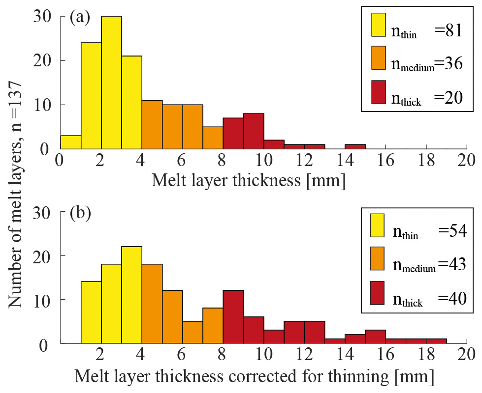
Figure A3 Histogram of melt layer thicknesses; the same color code is used as in Fig. 7. (a) Measured values and (b) values corrected for thinning using the thinning function from Gerber et al. (2021).

We see that most melt layers (n=81, Fig. A3a) are thin melt layers (M<4 mm, yellow). Even after correcting for thinning, this remains the same (Fig. A3b). Thick melt layers (M>8 mm, red) remain the rarest, although their number doubles when correcting for thinning. We find 40 thick melt layers in almost 10 000 years, giving an average of one big melt layer in 250 years. On average, we find one melt layer every 70 years, but not regularly (compare to Fig. 7).

A6 Too-thin melt layers

The time-averaged total melt record is corrected for thinning and for layers that are potentially missed due to core breaks (Fig. 7e, f). For consistency, we cut out layers that are thinner than 1.54 mm. This is the thickness of the thinnest layer found in the oldest section, with an age of 8101 years b2k (Fig. A4a, pink circle). We apply this threshold to thinning-corrected layers (Fig. A4a, pink line). Excluding these thin layers from older ice removes the bias from counting more thin layers in younger sections compared to older sections.

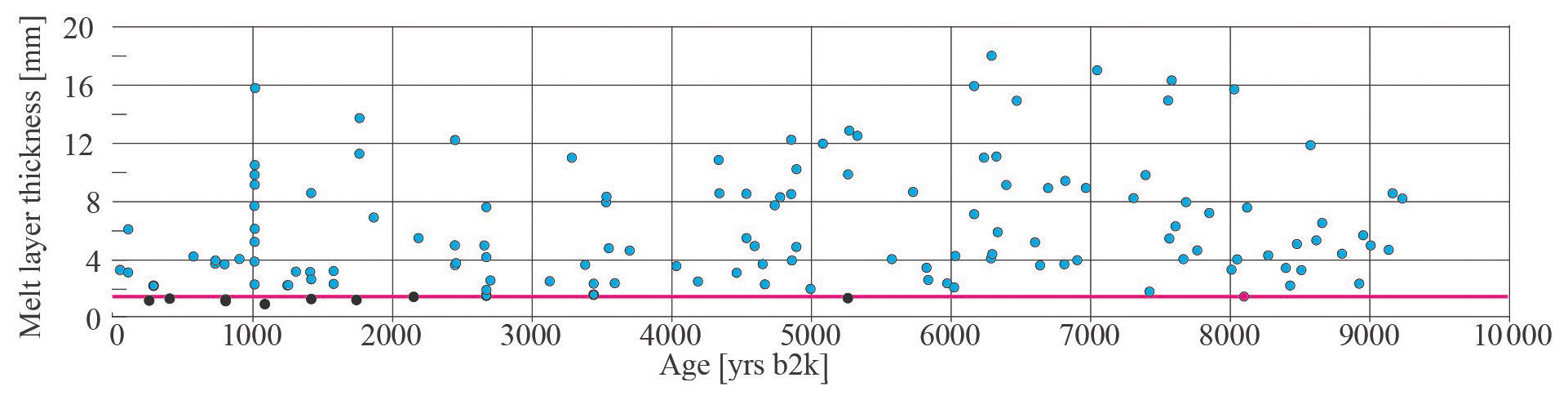
Figure A4 Thinning-corrected melt layer thicknesses (circles). Black circles were removed from the record due to the cutoff at 1.54 mm (pink circle and line).

A7 Melt layer and lens frequency

We analyze the duration between melt layers and melt lenses, representing the time from an event to the next younger event (Fig. A5). We distinguish between melt layers (blue bars, Fig. A5a) and melt lenses (green bars, Fig. A5b). Running means for 2-, 10-, and 50-year events show the long-term variations. As melt lenses are approximately three times more frequent, their spacing is much smaller than that of melt layers.

Figure A5 Time from an event to the next younger event for (a) 137 melt layers (vertical blue bars) and (b) 424 melt lenses (green bars). Different running means (averages with a moving window) are shown to visualize long-term variations. Red bars highlight periods with short spacing between events, and blue bars represent long spacing. Figure A6d shows the combination of melt layers and lenses.

In Fig. A5b (melt lenses), we see that around 1000, 3500 to 4000, 4500 to 5500, 6000, 8000 to 8200, and 500 years b2k, the time between two melt lenses is between 10 and 15 years (orange running mean), and therefore very short (red bars). We find a very large spacing (blue bars) of events around 500 years b2k, where the spacing exceeds 100 years, and in the period from 3000 to 3500 years b2k, where the spacing between two melt lenses is around 60 years. Such a large spacing between two melt lens events only becomes visible again in ice older than 9000 years, where bubble-free layers become more difficult to see and we end our analysis.

A similar pattern is also visible in Fig. A5a (melt layers), although with fewer details, as melt layers occur less frequently. Time spans with high melt lens frequencies roughly match periods with high frequencies of melt layers. A notable difference is seen for the period from 5800 to 6200 years b2k, where the time between two melt lenses is short but that between melt layers is long. The opposite is visible around 6400 years b2k, where the time between two melt layers is short but that between the lenses is long.

In both records (Fig. A5a, b), we find three shorter time spans (around 7800, 8100, and 8500 years b2k) that have a very short spacing between two events.

The long-term trend (Fig. A5b, purple line), which is the running mean over 50 events, suggests that the largest spacing between two events (approximately 30 to 35 years) occurs around 3000 years b2k, and the smallest spacing (12 years) occurs around 5000 years b2k. Going further back than 5000 years b2k, the trend gradually increases (i.e., the spacing between two melt events increases), with a small drop observed around 7500 years b2k. The largest spacing (35 years) between two events is reached at the very bottom of our analyzed depth range – older than 9000 years, where the likelihood of missing an event greatly increases.

A8 The climatic picture of the Holocene derived from melt events

Our climatic interpretation of Holocene summer temperatures (Fig. A6a) is derived, by eye, from the number of melt events, their thicknesses, and the melt event frequency (Fig. A6b, c, d respectively). In the central northeastern part of the Greenland ice sheet, i.e., the EastGRIP site, we see strong variations in these melt layer proxies over time, suggesting a fluctuating summer temperature over the past 10 000 years. The most recent 4000 years show a gradual decrease in melt events, with the last peak – probably caused by a single event – occurring around 1000 years before today. The trend in the Middle and Early Holocene appears to plateau, with some fluctuations. This climatic interpretation fits well with the generally accepted theory that summer temperatures decrease throughout the Holocene, e.g., Axford et al. (2021), and also follows the trend in stable water isotopes, a proxy for temperature (Fig. A6a). As melt events generally occur during summer, our interpretation is consistent with recent results from Bova et al. (2021) indicating that annual temperatures increase and summer temperatures decrease throughout the Holocene.

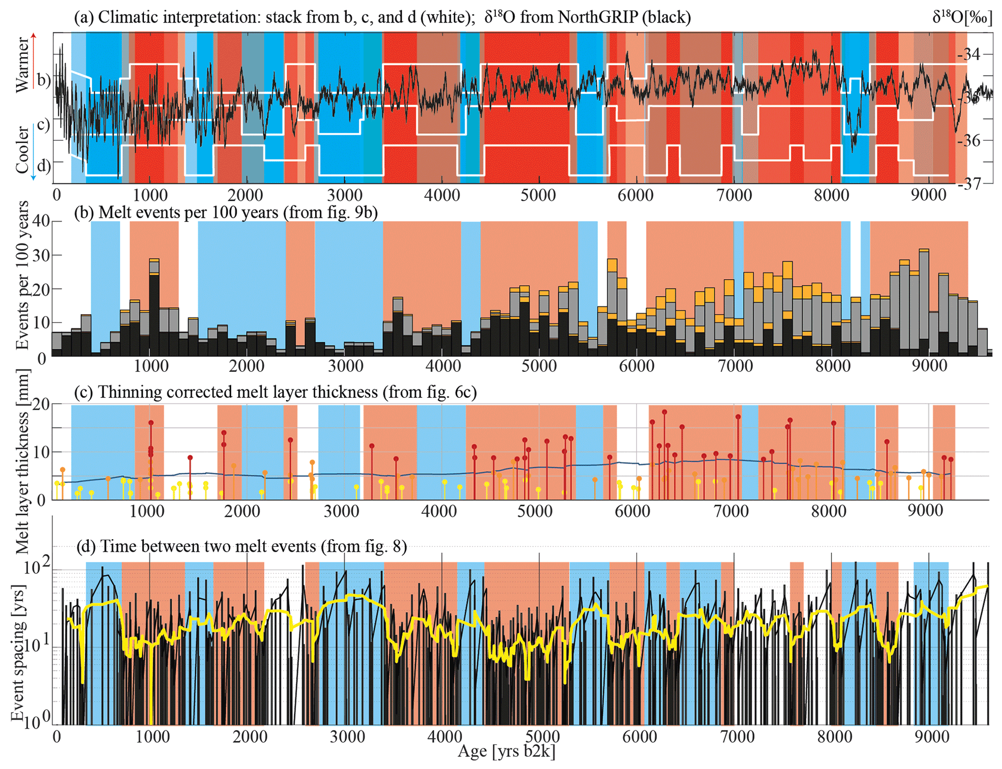
Figure A6 (a) A climatic interpretation of Holocene summer temperatures from the melt layer distribution over the Holocene. Without providing absolute values, red represents warmer periods and blue colder ones. The white lines are climatic interpretations from (b), (c), and (d), and the red and blue shading represents (b), (c), and (d) stacked. The stable oxygen isotope (δ¹⁸O) record from NorthGRIP is shown in black (North GRIP members, 2004). (b) Melt events per 100 years (Fig. 6b), with red shading indicating periods with many events and blue indicating periods with fewer events. (c) Melt layer thickness (Fig. 7c), with red shading indicating periods with thick melt layers. (d) Melt event frequencies, with short time spans between melt events shown in red and long time spans in blue. The running mean is shown in yellow.

We clearly see the Medieval Warm Period at around 1000 years b2k, identified by a number of melt layers and lenses. Concerning the Roman Warm Period, only the second half (2000 to 1600 years b2k) is visible in the number of melt events and the melt layer thickness (Fig. A6b and c, respectively), while the full period (between 2250 and 1600 years b2k) is represented by melt event frequencies (Fig. A6d). Based on Fig. A6a, we see the warm HCO occurring from 5800 to 7000, from 7200 to 8100, and from 8500 to 8700 years b2k, with cooler periods in between.

We find distinct cold periods around 500, 3000, 5600, and 8200 years b2k. In all our measurements (Fig. A6), the 8.2 kyr event (Alley et al., 1997; Thomas et al., 2007; Rasmussen et al., 2007) stands out as a period with very few melt events and only one melt layer. Our analysis does not show the 9.3 kyr event, as this is where we lose the signal due to the bubble–hydrate conversion.

Periods that are neither explicitly warm nor cold (e.g., the very recent past, i.e., younger than 100 years b2k) are shown in white (Fig. A6). During the youngest 100 years in our record, we see a clear increase in the stable water isotope signal (North GRIP members, 2004, Fig. A6a), showing an increase of temperature over the Greenland ice sheet. We remind the reader that our melt layer analysis ends in the year 1956 CE. For the more recent period, we rely on other data sources, e.g., Steen-Larsen et al. (2011), who suggest that we have had five melt events in the past 15 years. These melt events are derived from satellite-based microwave observations, and their existence in the snowpack is not confirmed, so they must be treated with caution. These five events would translate to 33 events per 100 years, and would create a peak slightly higher than the one at around 1014 years b2k, which we refer to as the 986 CE event from here on.

A9 Tree ring statistics

We test the hypothesis that warmer periods contain more melt events than colder ones (Fig. A7). For this, we remove outliers and test the amount of melt per decade (in the last 2500 years) against Poisson distributions. We find that in the 50 warmer decades, the occurrence of melt is 0.82 events per decade, while in the other decades it is on average 0.55. However, the attribution of warm/cold depends on the N-Tree record used as a temperature proxy, so we are forced to stop our analysis at 2500 years b2k. For the rest of the Holocene, we observe that the occurrence of melt is highest in the older millennia (4000 to 8000 years b2k) – on average about 1.5 per decade, compared to about 0.7 in the younger Holocene millennia (compare to Fig. 7f).

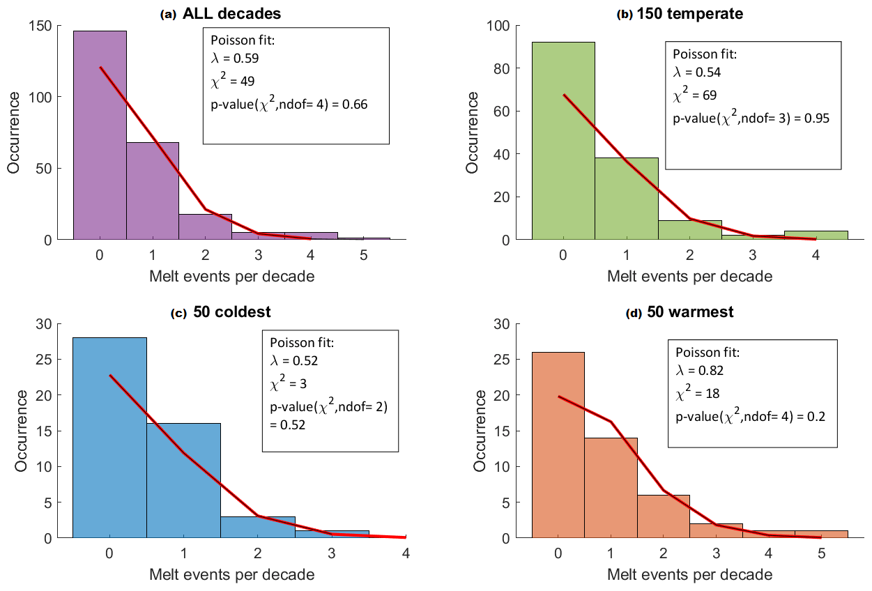
Figure A7 Histograms of melt events per decade over the last 2500 years. To highlight the correlation between melt and Northern Hemisphere temperatures, we distinguish between cold, warm, and temperate decades (b, c, and d, respectively). We fit the occurrence of melt per decade to Poisson distributions and obtain satisfactory p-values. The warmest decades (d) show an occurrence of melt that is 18 % higher than the general value (a). Melt in cold decades is not substantially different from the temperate value.

A10 Comparison to other melt layer records

A10.1 GISP2

To compare with our work, we use the only other melt layer record from a central Greenland ice core covering large parts of the Holocene. Alley and Anandakrishnan (1995) analyzed the GISP2 ice core using visual inspection and, to some degree, photography, the state-of-the-art method at that time. On average they found one melt event every 153 years. We find one melt event every 17.3 years in the EastGRIP ice core (561 melt events in total, Fig. 5c). We attribute the factor of 10 difference between these results to the better optical methods used nowadays.

The GISP2 (Alley and Anandakrishnan, 1995) and EastGRIP (this work) sites are both in a central region on the Greenland ice sheet, and the ice recovered at EastGRIP, inside the NEGIS, originates upstream from the GRIP and GISP2 area (Gerber et al., 2021). When ice flows downstream, the site elevation decreases and the temperature gradually increases (see the “Discussion”). For the Early Holocene, we can therefore assume that the records must be similar in some ways but that the number of events should gradually increase towards the present day. This holds, as the GISP2 record has a very pronounced HCO (between 6000 and 8000 years b2k), while our record (of certain events, Fig. 5c, dark colors) shows melt events to be slightly more evenly distributed over the past 10 000 years. When we include uncertain events (Fig. 5c, bright colors), the GISP2 and EastGRIP records are very similar and their peaks align well.

At site A in Greenland (70.8^∘ N, 36.0^∘ W, 3145 m), which is southeast of GISP2 and approximately 2 ^∘C warmer, Alley and Koci (1988) find nine melt events in the last 300 years. This relates to one event every 33 years at a site that is 2^∘ warmer than GISP2. Alley and Anandakrishnan (1995) argue that a value of one event per 33 years, rather than one event every 153 years, corresponds to a temperature increase of 2^∘. As this value was not reached in their record, they assume that the temperature variations throughout the Holocene must have been below 2^∘.

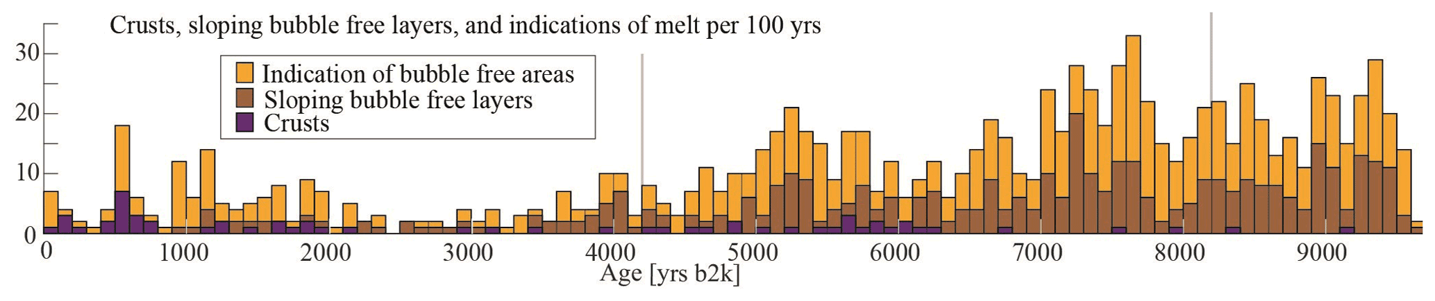
Figure A8 Number of bubble-free layers and lenses per century throughout the last 9700 years in the EastGRIP ice core. Indications of bubble-free areas, which are very uncertain melt layers and lenses that only hint at bubble-free areas, are shown in orange. Sloping bubble-free layers with a tilt of more than 10^∘ from the horizontal, which are in general very thin and not always continuous, are shown in brown. Crusts are shown in purple. Certain/clearly identifiable crusts only occur in the last 2000 years (upper 250 m). Crusts occurring beyond the last 2000 years were thought to be crusts during analysis but were later changed to uncertain melt layers. Note that the bar representing the period from 0 to 100 years b2k represents only 56 years, not 100 like the other bars, as our analysis begins in 1956 CE.

A10.2 RECAP ice core

Another available, but not peer reviewed, melt layer record has been assembled by Taranczewski et al. (2019) from the RECAP ice core. The authors present a melt layer record for the last 10 000 years in Renland, eastern Greenland. In this ice core, the Holocene covers 533 of the 584 m of total core length (Simonsen et al., 2019). As the Holocene ice reaches almost to bedrock, it is subject to high amounts of thinning in the bottom parts. As thinning equally affects bubble-free ice and bubbly ice (for ice, no study has shown the opposite so far), the signal is lost at a much shallower depth than at EastGRIP or GISP2. The RECAP record, therefore, provides a very robust melt layer record for the Late Holocene (the past 4200 years), but probably not for the Middle and Early Holocene.

Taranczewski et al. (2019) find a broad peak of melt events around 4000 years b2k, which is not visible in the GISP2 (Alley and Anandakrishnan, 1995) or EastGRIP (this study) melt layer records. The RECAP melt layer record is thus likely a regional record of eastern Greenland, but is not fully comparable with the central ice sheet.

A11 Indications of bubble-free layers, crusts, and sloping layers

Other than melt events, we find crusts, sloping bubble-free layers, and indications of melt events (Fig. A8). In total, we find 60 crusts (purple in Fig. A8), 17 of which we are certain about. These certain crusts are all found in the last 2000 years, i.e., the upper 250 m. Crusts found below this depth are classified as uncertain and were added as uncertain melt layers. We find 410 cases of sloping bubble-free layers, mainly at depths below 600 m (approximately 5000 years b2k). These bubble-free layers with an inclination of over 10^∘ are discussed in Sect. A12​​​​​​​. We also find 579 cases where the line scan images hint at an area or layer without bubbles that cannot be seen with full certainty. These are not included in our analysis and interpretation in the main text. These indications of bubble-free layers could represent warm summer days on which small amounts of surface melt occurred, but not sufficient melt to classify it as melting. This small amount of water at the air–ice interface can cause a change in the porosity of the firn. Dash et al. (2006) describe this as enhanced pre-melting, and discuss incomplete vs. complete surface melting. These pre-melt events are hard to identify in line scan images, or even under a microscope, and only become visible when comparing the brightness changes over a long section (>10 cm). We, therefore, classify these brightness changes as “very uncertain melt layers” or, as in Fig. A8, as “indications of bubble-free layers.” They are added to the overview for the sake of completeness and might be useful for comparison to other methods (e.g., Morris et al., 2021).

A12 A first attempt to interpret sloping bubble-free layers

Sloping bubble-free layers (Fig. A9) become more frequent in the lower half of our investigated depth range, i.e., below 600 m or older than 5000 years b2k (Fig. A8). These are layers that have a tilt of greater than 10^∘ (mostly between 30 and 60^∘) from the horizontal (Fig. A9). In general, they are discontinuous, giving them the appearance of a lens rather than a layer. These thin and hard-to-see structures are very dependent on which plane was cut, by chance, to produce the 2D line scan image (Westhoff et al., 2020). A layer such as that in Fig. A9 can easily be missed if it is located just a few millimeters below the surface.

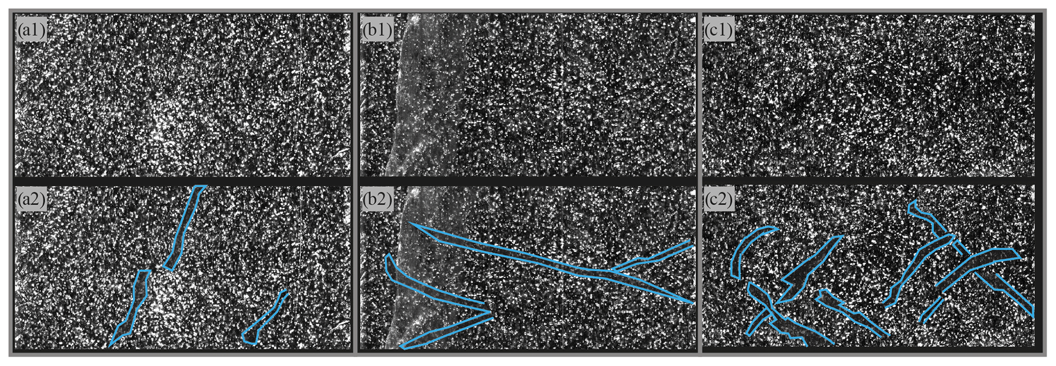
Figure A9 (a1, b1, c1) Line scan images and (a2, b2, c2) the same images as in the top row but with sloping bubble-free layers highlighted. (a) 459.60 m, 3840 years b2k, very steep structures, melt-pipe-like appearance. (b) 696.26 m, 5886 years b2k, continuous bubble-free structure appearing as a set of conjugate deformation bands. (c) 998.73 m, 8625 years b2k, many sloping bubble-free layers that are all at angles of around 45^∘.

These layers cannot be leftovers of sloping surface structures due to their steep tilt. Resolving the initial shape of the layer, i.e., by stretching it in the vertical, would cause the layers to become even steeper – too steep for ice sheet surface structures.

Figure A9a is an almost vertical structure and thus could be a melt pipe. Yet, this fails to explain why we only see these structures at great depths and not in the upper half of our depth range of interest.

Sloping layers at around 15^∘ and 45^∘ in Fig. A9b and c, respectively, appear to be sets of conjugate bands; thus, they could be the result of rheology. Steinbach et al. (2016) and Llorens et al. (2017) show sets of conjugate shear bands as a result of pure shear in ice in their numerical simulations. So far, in nature, all sloping layers allocated to deformation have been the result of simple shear (Alley et al., 1997; Jansen et al., 2016) and not pure shear. One challenge is that we expect to find shear bands where ice is softer, and thus brighter, due to more bubbles. Our results show that these shear bands appear in dark, bubble-free layers, contradicting the established theory. While discussing these deformation structures in detail is beyond the scope of this work, it is worth mentioning them for future investigations.