Climate and ice sheet evolutions from the last glacial maximum to the pre-industrial period with an ice-sheet–climate coupled model

The last deglaciation offers an unique opportunity to understand the climate–ice-sheet interactions in a global warming context. In this paper, to tackle this question, we use an Earth system model of intermediate complexity coupled to an ice sheet model covering the Northern Hemisphere to simulate the last deglaciation and the Holocene (26–0 ka). We use a synchronous coupling every year between the ice sheet and the rest of the climate system and we ensure a closed water cycle considering the release of freshwater flux to the ocean due to ice sheet melting. Our reference experiment displays a gradual warming in response to the forcings, with no abrupt changes. In this case, while the amplitude of the freshwater flux to the ocean induced by ice sheet retreat is realistic, it is sufficient to shut down the Atlantic meridional overturning circulation from which the model does not recover within the time period simulated. However, with reduced freshwater flux we are nonetheless able to obtain different oceanic circulation evolutions, including some abrupt transitions between shut-down and active circulation states in the course of the deglaciation. The inclusion of a parameterisation for the sinking of brines around Antarctica also produces an abrupt recovery of the Atlantic meridional overturning circulation, absent in the reference experiment. The fast oceanic circulation recoveries lead to abrupt warming phases in Greenland. Our simulated ice sheet geometry evolution is in overall good agreement with available global reconstructions, even though the abrupt sea level rise at 14.6 ka is underestimated, possibly because the climate model underestimates the millennial-scale temperature variability. In the course of the deglaciation, large-scale grounding line instabilities are simulated both for the Eurasian and North American ice sheets. The first instability occurs in the Barents–Kara seas for the Eurasian ice sheet at 14.5 ka. A second grounding line instability occurs ca. 12 ka in the proglacial lake that formed at the southern margin of the North American ice sheet. With additional asynchronously coupled experiments, we assess the sensitivity of our results to different ice sheet model choices related to surface and sub-shelf mass balance, ice deformation and grounding line representation. While the ice sheet evolutions differ within this ensemble, the global climate trajectory is only weakly affected by these choices. In our experiments, only the abrupt shifts in the oceanic circulation due to freshwater fluxes are able to produce some millennial-scale variability since no self-generating abrupt transitions are simulated without these fluxes.

1 Introduction

The Quaternary has been marked by large sea level oscillations. A gradual sea level fall, associated with an increase in the continental ice sheet volume, characterises prolonged glacial periods lasting for several tens of thousand of years. In turn, short glacial terminations precede interglacial periods that show reduced ice sheets. The study of glacial terminations can help us to understand the mechanisms behind large-scale ice sheet retreat but also the key role of ice sheets within the global climate system.

During the last deglaciation (∼21–7 ka), the sea level rose by about 120 metres to reach approximately its present-day level (Waelbroeck et al., 2002; Lambeck et al., 2014). This rise is mostly explained by the disintegration of the North American and Eurasian ice sheets, while Greenland and Antarctica together probably contributed less than 20 m (Whitehouse et al., 2012; Briggs et al., 2014; Lecavalier et al., 2014; Simms et al., 2019). The extent of the Northern Hemisphere ice sheets across the deglaciation is relatively well known, although it can sometimes present large (>1 kyr) dating uncertainties (Hughes et al., 2016; Dalton et al., 2020). However, the volume evolution of the individual ice sheets remains weakly constrained. In particular, sea level archives have suggested the presence of abrupt sea level rises standing out from the gradual sea level rise of the deglaciation (Deschamps et al., 2012; Abdul et al., 2016; Harrison et al., 2019). These so-called meltwater pulses suggest large-scale ice sheet instabilities, but the contribution of the different ice sheets to these events remains debated (e.g. Liu et al., 2016).

Parallel to the non-linear ice sheet retreat, the atmosphere and the ocean have also undergone some large and abrupt variations. For example, while atmospheric temperatures above Greenland rise gradually since the Last Glacial Maximum (LGM), they rise abruptly by more than 10 ^∘C in a few decades at the onset of the Bølling–Allerød period at 14.7 ka (Severinghaus and Brook, 1999; Buizert et al., 2014). After 500 years of interglacial conditions, the climate abruptly returns to a cold state during the Younger Dryas (Alley, 2000a) from which the temperatures rise again steadily to reach their Holocene values. The evolution of the oceanic conditions are more uncertain. It seems nonetheless that the North Atlantic Deep Water (NADW) was shallower at the LGM compared to today (Curry and Oppo, 2005). The 3D evolution of the water masses across the deglaciation is difficult to constrain given that different proxies can provide conflicting information (Waelbroeck et al., 2019). However, it is likely that the Atlantic meridional oceanic circulation (AMOC) has not remained constant, with possible rapid transitions from different states: intense, reduced or even shut down (e.g. McManus et al., 2004; Ng et al., 2018).

The succession of events linking the changes in the atmosphere, ocean and ice sheets has yet to be formalised. Bi-directionally coupled ice-sheet–climate models are ideal tools to study these interactions since they can explicitly represent the different climatic feedbacks at play, without having to prescribe ad hoc external scenarios. In such coupling, the climate model provides the climatic forcing fields needed by the ice sheet model and in turn the ice sheet model provides an updated surface topography and ice sheet mask. Several coupled ice-sheet–climate models are now available in the literature, spanning a range of complexities. Given that the ice sheet integrates climate change over long timescales (>10 kyr), the vast majority of the work that has investigated multi-millennial climate change during the Quaternary has used simplified climate models to reduce the numerical cost (e.g. Calov et al., 2005; Fyke et al., 2011; Huybrechts et al., 2011; Heinemann et al., 2014). However, some general circulation models (GCMs) have also been bi-directionally coupled to ice sheet models (e.g. Vizcaíno et al., 2008; Gregory et al., 2012). In this case, the model is run for short integrations (typically less than 1000 years) or use an asynchronous coupling to speed up the simulations (e.g. Ziemen et al., 2019). With the asynchronous coupling, the climate model is run less frequently than the ice sheet model (e.g. 1 year of climate is used to perform 10 years of ice sheet evolution).

To date, although a fair amount of coupled ice-sheet–climate models exist, only few have been used to simulate the last deglaciation of Northern Hemisphere ice sheets. Thanks to an inexpensive setup in terms of computational cost, the CLIMBER-2 Earth system model of intermediate complexity coupled to the SICOPOLIS ice sheet model has been used in several studies to simulate the last glacial–interglacial cycles (e.g. Ganopolski and Brovkin, 2017) and beyond (Willeit et al., 2019). CLIMBER-2 has also been coupled to an alternative ice sheet model (Charbit et al., 2005; Bonelli et al., 2009). These studies have demonstrated the ability of the model to reproduce the global eustatic sea level reconstructions. They have also brought major improvements in our understanding of the respective role of orbital forcing, greenhouse gas mixing ratio, ice sheets and dust to explain the past climatic variability. However, CLIMBER-2 shows drastic simplifications of the physics of the atmosphere (statistical–dynamical model on a coarse grid of $\mathrm{10}{}^{\circ }\times \sim \mathrm{51}{}^{\circ }$ resolution) and in the ocean (three zonally averaged oceanic basins). Heinemann et al. (2014) used an alternative Earth system model of intermediate complexity, LOVECLIM (Goosse et al., 2010), to simulate the last deglaciation of Northern Hemisphere ice sheets. Compared to CLIMBER-2, LOVECLIM shows a higher spatial resolution in the atmosphere ($\sim \mathrm{5.6}{}^{\circ }\times \mathrm{5.6}{}^{\circ }$ resolution) and accounts for a general circulation oceanic model (Goosse and Fichefet, 1999). To successfully reproduce the ice sheet evolution Heinemann et al. (2014) have to use a correction of the climatic fields (namely temperature and precipitation). In addition, they use an asynchronous coupling to speed up their simulations. In doing so, they discard the role of freshwater flux to the ocean resulting from ice sheet melting. To our knowledge, no other bi-directionally coupled ice-sheet–climate model has been used to simulate the last deglaciation of Northern Hemisphere ice sheets.

Building on the work of Roche et al. (2014a), we present here the first comprehensive climatic simulations of the last deglaciation with interactive Northern Hemisphere ice sheets using a bi-directional synchronous coupling. We have performed different experiments with varying oceanic conditions to assess their importance in shaping the deglaciation. In addition, we have performed additional sensitivity experiments using an asynchronous coupling to assess the importance of some modelling choices on our results. In Sect. 2 we present our model, the coupling strategy and the experimental setup. We show our results in terms of atmospheric temperature evolution, oceanic circulation changes and simulated ice sheets in Sect. 3. We discuss further our model limitations and expected improvements in Sect. 4 and conclude in Sect. 5.

2 Methods

2.1 Climate and ice sheet models

iLOVECLIM (here in version 1.1) is a code fork of the LOVECLIM 1.2 model (Goosse et al., 2010). The core of the model is a combination of a quasi-geostrophic atmospheric model solved on a T21 ($\sim \mathrm{5.6}{}^{\circ }\times \mathrm{5.6}{}^{\circ }$) spectral grid (ECBilt, Haarsma et al., 1997; Opsteegh et al., 1998); a free surface oceanic general circulation model on a $\mathrm{3}{}^{\circ }\times \mathrm{3}{}^{\circ }$ spherical grid which includes a thermodynamic sea ice model (CLIO, Goosse and Fichefet, 1999); and a dynamic vegetation and carbon allocation model (VECODE, Brovkin et al., 1997). iLOVECLIM has been extensively used to study millennial climate change during the Quaternary. For example, it has proven able to reproduce the glacial–interglacial variability of the hydrological cycle in the tropics (Caley et al., 2014). It has also been used to study Heinrich events during the last glacial period (Roche et al., 2014b) or to investigate the processes responsible for changes in the carbon cycle during the last eight interglacial periods (Bouttes et al., 2018). With a similar model configuration to the one used in this work, iLOVECLIM results were included in the fourth phase of the Palaeoclimate Modelling Intercomparison Project (PMIP) contribution to the Coupled Model Intercomparison Project (CMIP) (Kageyama et al., 2021).

Since Roche et al. (2014a), the model has also included a 3D thermomechanically coupled ice sheet model (GRISLI, Ritz et al., 2001; Quiquet et al., 2018a). GRISLI solves the ice sheet mass conservation equation on a Cartesian grid. Like most ice sheet models, deformation is computed with a Glen flow law in which anisotropy is artificially accounted for using a flow enhancement factor (E_f) that facilitates deformation induced by vertical shear. For the entire domain, the velocity field is the sum of velocity driven by vertical shearing (shallow ice approximation, SIA) and the velocity driven by horizontal shearing (shallow shelf approximation, SSA). In doing so, the SSA is used as a sliding law (Bueler and Brown, 2009; Winkelmann et al., 2011). Basal dragging τ_b is assumed to follow a linear friction law:

$$\begin{array}{}\text{(1)}& {\mathit{\tau }}_{\mathrm{b}}=-\mathit{\beta }{\mathit{u}}_{\mathrm{b}},\end{array}$$

where β is the basal drag coefficient and u_b is the basal velocity. Cold-based grid points have a virtually infinite friction at the base (5×10⁵ Pa yr m⁻¹), while floating ice shelves have no friction. For grid points at the pressure melting point, we use a friction computed from the effective pressure at the base of the ice sheet N:

$$\begin{array}{}\text{(2)}& \mathit{\beta }=c_{\mathrm{f}}N,\end{array}$$

where c_f is a parameter that has to be calibrated. For the experiments shown here, we impose an ice flux at the grounding line that follows the analytical solution of Tsai et al. (2015). Calving at the ice shelf edge occurs if the ice thickness falls below a critical threshold and if the upstream Lagrangian ice flux does not allow us to maintain an ice thickness above this threshold. The threshold is set here to 250 m. Ice sheet model parameters (enhancement factor, basal drag coefficient and hydraulic conductivity) are calibrated in the same way as in Quiquet et al. (2018a) to reproduce glacial–interglacial Antarctic ice sheet grounding line migration. In addition, we used a map of sediment thickness (Laske and Masters, 1997) to locally reduce basal dragging. We assume that for a sediment thickness greater than 200 m, the basal drag coefficient in Eq. (2) is multiplied by a dimensionless factor of 0.05. Glacial isostatic adjustment is accounted for in GRISLI using an elastic-lithosphere–relaxed-asthenosphere model (Le Meur and Huybrechts, 1996), with a relaxation time of the asthenosphere of 3000 years. The ice sheet model is run here on a Cartesian 40 km grid of the Northern Hemisphere using a Lambert azimuthal equal-area projection.

2.2 Ice sheet model coupling

The inclusion of GRISLI into iLOVECLIM has been presented in Roche et al. (2014a). However, the coupling procedure has been largely modified from this work. In particular, we have substantially improved the computation of surface and sub-shelf mass balance. Water conservation between GRISLI and the rest of the climate model has also been considerably improved. Details on this coupling are given in the following, while its schematic representation is shown in Fig. 1. It is important to mention that only the Northern Hemisphere ice sheets are interactively simulated, while the Antarctic ice sheet topography and ice mask remain prescribed at their Last Glacial Maximum following the PMIP4 protocol.

Figure 1 Schematic representation of the coupling between the ice sheet model (GRISLI) and the atmospheric (ECBilt) and the oceanic (CLIO) models.

2.2.1 Surface mass balance

In Roche et al. (2014a), the ice sheet surface mass balance (SMB) was computed from the annual mean precipitation and the annual and July mean near-surface air temperature using a positive degree day method (Reeh, 1989). Although computationally inexpensive and easy to implement in a model, this method does not account for some important physical quantities that influence the SMB. In particular, the surface shortwave radiation is only implicitly taken into account through the temperature. Instead, we use here the insolation temperature melt method (ITM) following Pollard (1980) and van den Berg et al. (2008). The amount of melt M_s over one time step Δt is in this case

$$\begin{array}{}\text{(3)}& M_{\mathrm{s}}=max\left({\displaystyle \frac{\mathrm{\Delta }t}{{\mathit{\rho }}_{\mathrm{w}}{L}_m}}\left(\left(\mathrm{1}-\mathit{\alpha }\right){\text{SW}}_{\mathrm{s}}+c_{\mathrm{rad}}+\mathit{\lambda }{T}_{\mathrm{s}}\right),\mathrm{0}\right),\end{array}$$

where is the T_s is the near-surface air temperature, SW_s is the shortwave radiation at the surface, α is the surface albedo, ρ_w is the density of liquid water and L_m is the specific latent heat of fusion. λ and c_rad are empirical parameters that need calibration. In the literature, this calibration has been performed on observations of present-day glaciers. The λ parameter is generally set to 10 W m⁻² K⁻¹ (Pollard, 1980; van den Berg et al., 2008; Robinson et al., 2010). The parameter c_rad is less constrained and is adjusted for the region considered (van den Berg et al., 2008). It is set to −50 W m⁻² in Pollard (1980), it ranges from −40 to −60 W m⁻² in Robinson et al. (2010), whilst it is equal to −117 W m⁻² in van den Berg et al. (2008). We used λ=10 W m⁻² K⁻¹ and $c_{\mathrm{rad}}=-\mathrm{40}$ W m⁻². However, iLOVECLIM presents an important warm bias in eastern North America and a cold bias in northern Europe that lead to an unrealistic simulated ice sheet under glacial forcing, a problem also identified in Heinemann et al. (2014). To account for this, we use a local modification of the melt parameter c_rad to partially correct these temperature biases. To this aim, we compute the annual mean temperature bias with respect to ERA-Interim (Dee et al., 2011) and use a linear correction in which a +10 ^∘C bias leads to $c_{\mathrm{rad}}=-\mathrm{80}$ W m⁻² (instead of the reference value of −40 W m⁻²).

Because of the gap between the coarse atmospheric model resolution and the ice sheet model resolution, the downscaling of the forcing fields needed by the ice sheet model is a persistent issue in ice-sheet–climate coupling. Here, we make use of the online dynamical downscaling embedded in iLOVECLIM (Quiquet et al., 2018b). This allows for the computation on every atmospheric model time step (4 h) of snow, rain and near-surface air temperature at the ice sheet model resolution, explicitly taking into account the high-resolution topography. We used these fields directly to compute a surface mass balance at the resolution of the ice sheet model with the ITM method (Eq. 3). The near-surface air temperature and the SMB are accumulated along the course of the year to generate the yearly forcing fields required by the ice sheet model. We made a few adjustments compared to the downscaling procedure presented in Quiquet et al. (2018b). In particular, some large-scale climate fields are now bi-linearly interpolated onto the high-resolution grid before the energy and moisture computation. This prevents the strong discontinuities that could exist between two sub-grid points belonging to two different large-scale grid cells.

2.2.2 Sub-shelf melt rate

The sub-shelf melt rate in Roche et al. (2014a) was imposed arbitrarily to a homogeneous and constant value for the entire Northern Hemisphere. Instead, we use here a physically based computation of the sub-shelf melt rate following Beckmann and Goosse (2003). For each vertical oceanic layer, z, we estimate the potential sub-shelf melt rate as

$$\begin{array}{}\text{(4)}& M_{\mathrm{shelf}}\left(z\right)={\displaystyle \frac{{\mathit{\rho }}_{\mathrm{w}}{c}_p{\mathit{\gamma }}_{\mathrm{T}}{F}_{\mathrm{g}}\text{TF}\left(z\right)}{{\mathit{\rho }}_{\mathrm{i}}{L}_m}},\end{array}$$

where c_p is the specific heat capacity of sea water, ρ_i is the density of ice, γ_T is the thermal exchange velocity and TF(z) is the thermal forcing at depth z, defined as the difference between the ambient temperature and the temperature of the salinity-dependent freezing point. F_g is a weakly constrained dimensionless parameter and can be changed to explore the response of the ice sheet to different sub-shelf melt sensitivities to oceanic temperature change. In our reference experiment, we chose a parameter value ($\mathrm{15}\times {\mathrm{10}}^{-\mathrm{3}}$) that produces about 0.1 m yr⁻¹ in the Arctic, a value similar to what the Ross ice shelf is experiencing today in Antarctica. In addition, in order to avoid unrealistic ice shelf expansion over the deep ocean we also impose a high sub-shelf melt rate of 20 m yr⁻¹ where the bathymetry is greater than 1500 m. Also, to mimic the fact that observed melt rates are greater in the vicinity of the grounding line, we double the value of the inferred melt rate in Eq. (4) for the floating points that are in contact with the grounding line. Equation (4) is computed for each oceanic time step (1 d) and integrated over the year in order to provide the yearly forcing needed by the ice sheet model. There is no downscaling of the sub-shelf melt rate to the high-resolution ice sheet model grid, except that the depth of the ice shelf draft is used to determine the vertical layer z in Eq. (4) that produces the melt.

2.2.3 Ice sheet feedbacks

Changes in the ice sheet feed back to the atmospheric and to the oceanic models. On the one hand, at the beginning of each year in the climate model, the ice mask and the orography in the climate model are changed according to the changes computed by the ice sheet model in the previous year. Both fields are aggregated from the ice sheet model resolution (40 km) to the T21 resolution in the same way as in Roche et al. (2014a). There is no partially glaciated grid cell in the atmospheric model: a coarse grid cell is regarded as glaciated (ice mask set to 1) if it contains at least 30 % of sub-grid points with an ice thickness greater than 1 m. The ice mask in the atmospheric model impacts the surface albedo.

On the other hand, freshwater fluxes resulting from the ice sheet melting are transferred to the oceanic model. In Roche et al. (2014a), the total ice sheet volume variation was transferred to the continental routing scheme assuming a uniform distribution over the ice sheet. Only the calving flux was separated from the total volume variation to eventually feed an iceberg model (Bügelmayer et al., 2015). This method has the advantage of ensuring a closed water budget within the model but the spatial information about ice sheet runoff is lost. For this reason, we now explicitly separate the different components of the global volume variation on the ice sheet model side. Basal and surface melt of the grounded part of the ice sheet are transferred to the routing scheme exactly where they occur. The basal melt below the ice shelves are also added to the ocean where they occur but at the surface and not at depth. The calving flux can be either regarded as the basal melt or used to feed the iceberg model. At present, the iceberg model is not activated in our experiments and the calving flux, similarly to the sub-shelf melt, is given at the oceanic surface. Local latent heat release resulting from iceberg melting is taken into account. Since the ice sheet model main time step is 1 year, we do not have access to the seasonal cycle of the freshwater fluxes and their annual value computed by the ice sheet model is homogeneously distributed through the year in the oceanic model.

For the experiments presented here, changes in the ice sheet size do not affect the global ocean volume. The bathymetry in the oceanic model thus remains constant.

2.3 Experimental setup

2.3.1 Boundary and initial conditions

The climate model uses time-varying information of greenhouse gases (Lüthi et al., 2008) and insolation (Berger, 1978). The carbon dioxide mixing ratio evolution and the 65^∘ N insolation in June is depicted in Fig. 3. For the oceanic model, we use a recent implementation of the Last Glacial Maximum bathymetry at 21 ka (Lhardy et al., 2021), which is left unchanged for the duration of the experiments. Topography and ice mask are both provided by the ice sheet model. On the ice sheet model side, in addition to the climate forcings, another forcing is the transient eustatic sea level reconstruction from Waelbroeck et al. (2002).

To define our initial state, we run uncoupled ice sheet and climate experiments. First, we run the climate model using the Last Glacial Maximum boundary conditions for 3000 years. In this case, the ice sheet topography and ice mask correspond to the one of the GLAC-1D reconstructions (Tarasov et al., 2012; Tarasov and Peltier, 2002; Briggs et al., 2014) at 21 ka. The different experiments presented in the rest of the paper are all branched from the simulated climate at the end of this 3000 years. In addition, the last 100 years of this experiment are also used to define a climatological annual surface mass balance and surface temperature. We use this climatology to perform stand-alone ice sheet experiments starting from an ice-free configuration of the Northern Hemisphere. The ice sheet model is run for 200 kyr under this constant climate forcing. In doing so, the model has time to build up ice sheets in equilibrium with the Last Glacial Maximum climate simulated by the climate model. We chose to run such a long spin-up so that the slowly evolving variables, such as the internal temperature field and the basal hydraulic head, are in equilibrium with the simulated glacial climate. In this way, we reduce the initial model drift for the coupled experiments. The simulated ice sheets after this spin-up are presented in Fig. 2a. The extent of the ice sheets generally agrees well with the geologically constrained reconstruction of GLAC-1D (Fig. 2c) and ICE-6G_C (Fig. 2d, Argus et al., 2014; Peltier et al., 2015) even though it is underestimated in the western part of the Eurasian ice sheet. The climate fields used to build the spun-up ice sheets have been elaborated from the climate model with prescribed GLAC-1D boundary conditions. As such, the spun-up ice sheets should resemble the GLAC-1D reconstructions. If this is generally the case, there is nonetheless an overestimation of the surface elevation of the North American ice sheet. This could indicate a precipitation overestimation in this area or an underestimation of the ice sheet velocities. However, the fact that the Eurasian ice sheet does not present this bias points towards an overestimation of the precipitation. The spun-up ice sheets are used as initial conditions for the ice sheet model in the coupled experiments presented in this paper. All the experiments, including the sensitivity experiments with perturbed parameter values, use the same spun-up climate and ice sheet states.

Figure 2 Surface elevation above contemporaneous sea level: (a) after the glacial spin-up, (b) in the reference deglaciation experiment DGL at 21 ka, (c) in the GLAC-1D reconstruction and (d) in the ICE-6G_C reconstruction. The colour scale is different for ice-free and ice-covered regions. The simulated ice sheet grounding line is represented by the red line, while the black lines represent isocontours of ice sheet surface elevation (separated by 1000 m).

2.3.2 Description of the experiments

We have performed two sets of experiments to investigate two important points for the simulation of the deglaciation. First, the freshwater fluxes resulting from ice sheet melting likely influenced the climate evolution during the deglaciation since they can have led to abrupt AMOC changes (e.g. Liu et al., 2009; Menviel et al., 2011; Obase and Abe-Ouchi, 2019). Thus, in a first set of experiments, we have performed various synchronously coupled experiments with varying oceanic circulation evolutions. Second, several modelling choices related to the ice sheet model are not well constrained and could also have an influence on the simulated deglaciation. To tackle this problem, in a second set of experiments, we have performed various sensitivity experiments using an asynchronous coupling to reduce the computation cost. More details on these experiments are given in the following.

Our reference experiment (DGL) is an ice-sheet–climate experiment, synchronously coupled. This experiment starts at 26 ka and uses the initial conditions presented in Sect. 2.3.1. The climate and the ice sheets used as initial conditions are not fully consistent between each other since they have been obtained with uncoupled long-term equilibriums. As such, the first 1000 years or so of our experiments have to be discussed with care since part of the response can arise from artefacts due to the start of the coupling.

In addition to this reference experiment, we have performed additional synchronously coupled experiments for the first set of experiments which aims at investigating the importance of oceanic changes in shaping the last deglaciation.

First, we have run experiments in which the amount of freshwater is reduced in order to gradually limit their influence. In DGL_FWF/2 and DGL_FWF/3 we divide the flux resulting from ice sheet melting by 2 and 3, respectively, while in DGL_noFWF this flux is not injected into the ocean.

Second, it has been shown that the simulated NADW at the LGM in the iLOVECLIM model is too deep with respect to what oceanic tracers suggest (Lhardy et al., 2021), a feature shared with other PMIP participating models (Kageyama et al., 2021). This bias in the oceanic circulation can affect our results for the deglaciation. One way to provide an alternative oceanic circulation in the model is to use a parameterisation for the sinking of brines (Bouttes et al., 2010) around Antarctica. In this parameterisation, a fraction of the salt rejected by sea ice formation (40 %) is transferred to the deepest oceanic layer. This is done to artificially reproduce the sinking of dense waters induced by sea ice formation along the continental slope of Antarctica since such a process cannot be properly resolved in a $\mathrm{3}{}^{\circ }\times \mathrm{3}{}^{\circ }$ resolution oceanic model. The parameterisation favours vertical stratification around Antarctica, enhancing Antarctic Bottom Water (AABW) and conversely weakening and shallowing of the NADW. Under glacial conditions, this leads to a better agreement with palaeo-data (Lhardy et al., 2021). We have thus performed an experiment in which the parameterisation for the sinking of brines is activated (DGL_brines). The experiments with reduced freshwater flux and with the parameterisation for the sinking of brines are branched from the reference experiment DGL at 21 ka. At that time the ice sheets are not contributing to sea level change (total mass change of 0).

The second set of experiments consists of asynchronously coupled experiments to assess the sensitivity of our results to the modelling choices for the ice sheet model. In these experiments, the forcings (greenhouse gas mixing ratio and orbital forcing) are accelerated with a factor of 5. Acceleration has already been used extensively in the literature (e.g. Jackson and Broccoli, 2003; Gregory et al., 2012; Roberts et al., 2014; Heinemann et al., 2014; Choudhury et al., 2020). The accelerated experiments cover the 26–0 ka time span, but only 5200 years are computed in the climate model instead of the full 26 000 years. In such experiments, the ice sheet model is run for 5 years after 1 year of simulated climate so that only the ice sheet forcings are accelerated but not ice dynamics. This method allows us to significantly reduce the computation time needed to perform multi-millennial experiments. However, accelerated experiments cannot correctly represent the effect of freshwater discharge to the ocean resulting from ice sheet melting since either the flux of water or the mass can be preserved but not both at the same time. Here, we discard completely the role of freshwater flux to the ocean in the accelerated experiments. The ADGL experiments are the accelerated counterpart of the DGL experiments and as such will define the new reference for the accelerated experiments.

The other accelerated experiments are used to assess the sensitivity of our simulated deglaciation to important processes related to ice sheet dynamics: modelling choices for ice dynamics, for the surface mass balance and for the sub-shelf melt rate.

First, we explore two aspects related to ice dynamics: grounding line dynamics and ice deformation. The ice sheet model GRISLI accounts for two formulations of the flux at the grounding line. For the Antarctic ice sheet, the use of Schoof (2007) instead of Tsai et al. (2015) leads to slower grounding line retreat during deglaciation phases (Quiquet et al., 2018a). For this reason, in the ADGL_schoof experiment we use the Schoof (2007) formulation of the flux at the grounding instead of Tsai et al. (2015). A second aspect for ice dynamics is the choice of the flow enhancement factor E_f, which is a tuned parameter that has consequences for the ice velocity. In the ADGL_ef experiment we use a larger flow enhancement factor (larger velocities) since the simulated North American ice thickness at the LGM is overestimated (Fig. 2).

Then, to explore the sensitivity of our results to the surface mass balance we have performed two experiments in which the weakly constrained melt parameter c_rad (Eq. 3) is changed. In ADGL_accplus we use a smaller value for this parameter in order to reduce surface melt to delay the deglaciation. In the ADGL_nocor experiment we use a homogeneous value of c_rad instead of using the spatial heterogeneous value defined from the temperature bias.

Finally, to assess the sensitivity of our results to the sub-shelf melt rate, in the ADGL_bmbplus we enhance the sub-shelf melt rate to increase the relative importance of oceanic changes with respect to atmospheric changes.

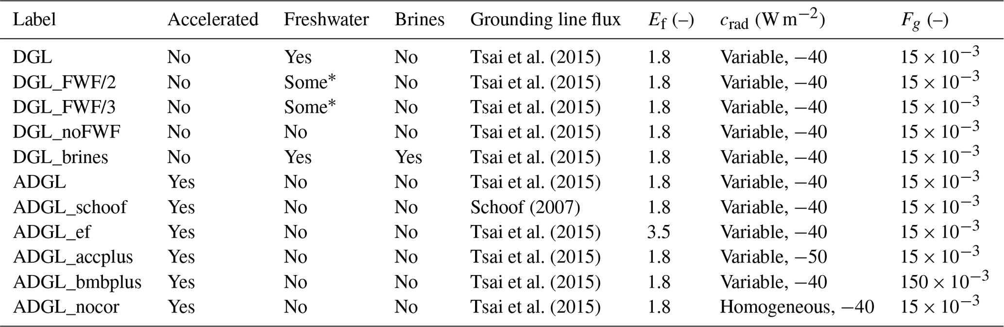
The list of the different experiments is available in Table 1.

Tsai et al. (2015)Tsai et al. (2015)Tsai et al. (2015)Tsai et al. (2015)Tsai et al. (2015)Tsai et al. (2015)Schoof (2007)Tsai et al. (2015)Tsai et al. (2015)Tsai et al. (2015)Tsai et al. (2015)

Table 1 Characteristics of the experiments performed in this study. The accelerated experiments use an ice sheet coupling frequency of 5 years with an acceleration factor for the forcings of 5. The freshwater flux to the ocean resulting from ice sheet melting is either considered (labelled “yes”), discarded (“no”) or partially considered (marked with ^*). Brine rejection due to Southern Ocean sea ice formation is either considered or not. The ice flux at the grounding line in the ice sheet model follows the Tsai et al. (2015) or the Schoof (2007) formulation. The calibrated value for the ice flow enhancement factor, E_f, is 1.8. The parameter c_rad in the surface melt model is −40 W m⁻² in the reference experiments, and its value is locally corrected with a map elaborated from the present-day annual mean surface temperature bias (labelled “variable”). The parameter F_g is used in the linear sub-shelf melt model, set in its reference value at $\mathrm{15}\times {\mathrm{10}}^{-\mathrm{3}}$.

The climate model computes about 850 years in 24 h on a single core of an Intel^®Xeon^®CPU@3.70 GHz. The computational cost of the ice sheet model is negligible with respect to the rest of the climate model, while the interactive atmospheric downscaling decreases the performance by about 40 % compared to the standard climate model. The coupled synchronous experiments took roughly 1 month to complete, while the asynchronous experiments were approximatively 5 times faster.

3 Results

In this section we first describe the general evolution of the simulated climate in the synchronously coupled experiments before examining the ice sheet changes. Then we examine the results for the accelerated asynchronously coupled experiments to infer the sensitivity of our results to different ice sheet evolutions.

3.1 Climate evolution in the synchronously coupled ice-sheet–climate experiments

The simulated global mean surface temperature evolution for the synchronously coupled ice sheet climate experiments is shown in Fig. 3, together with the strength of the AMOC. In response to the forcings, the different experiments produce a gradual warming from the Last Glacial Maximum towards its maximum value during the Holocene. The glacial–interglacial temperature difference ranges from 3.1 to 3.8 ^∘C and is in good agreement with a palaeo-temperature stack (Shakun et al., 2012), even though iLOVECLIM is one of the warmest models at the LGM within the PMIP4 ensemble (Kageyama et al., 2021). The glacial–interglacial temperature difference is mostly explained by the cold temperatures at the LGM resulting from the large ice sheets that induce higher surface elevations and a strong albedo effect. A polar amplification is simulated since the northern and southern high latitudes both show a greater temperature difference from the pre-industrial period compared to the tropics (Fig. 4). This pattern is consistent with recent reconstructions (e.g. Tierney et al., 2020, shown in Fig. 4d), even though with a smaller amplitude in our model. However, our simulated glacial–interglacial temperature difference is within the range of other estimates (4±0.8 ^∘C, Annan and Hargreaves, 2013).

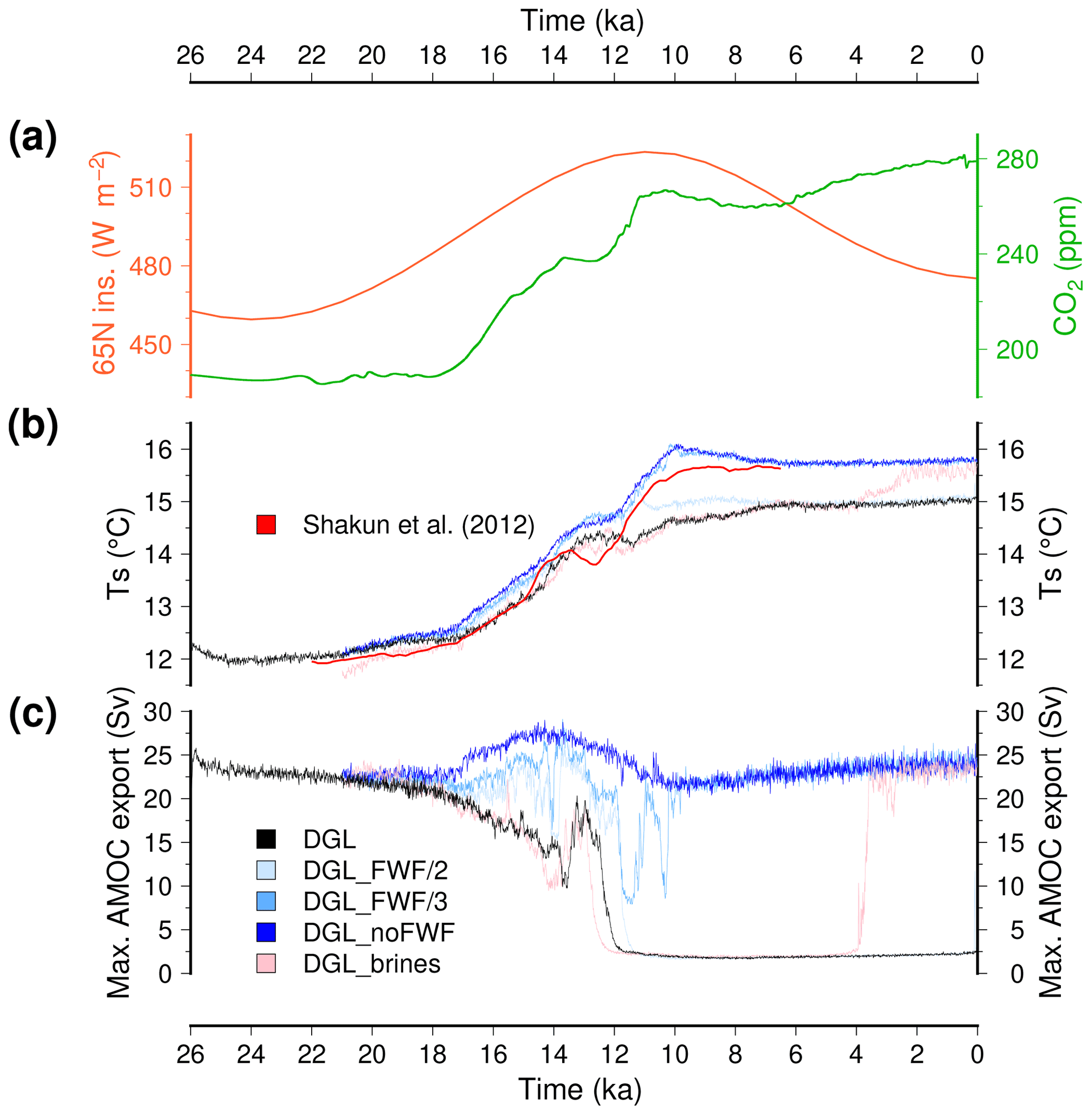
Figure 3 (a) Time evolution of the major forcings for the climate model (June insolation at 65^∘ N and carbon dioxide mixing ratio). (b) Simulated global mean surface temperature. (c) Simulated maximum of the Atlantic stream function. The reference model DGL is in black, while the experiments with reduced freshwater flux to the ocean from ice sheet melting are depicted with blue shading (dark blue for no freshwater flux). The experiments with enhanced brine formation are in pink. Here, we use a 10-year running mean for the model results to smooth interannual variability. In (b) we also show the temperature anomaly reconstruction from Shakun et al. (2012) (to which we added 15.5 ^∘C, a typical pre-industrial global mean surface temperature simulated by the model).

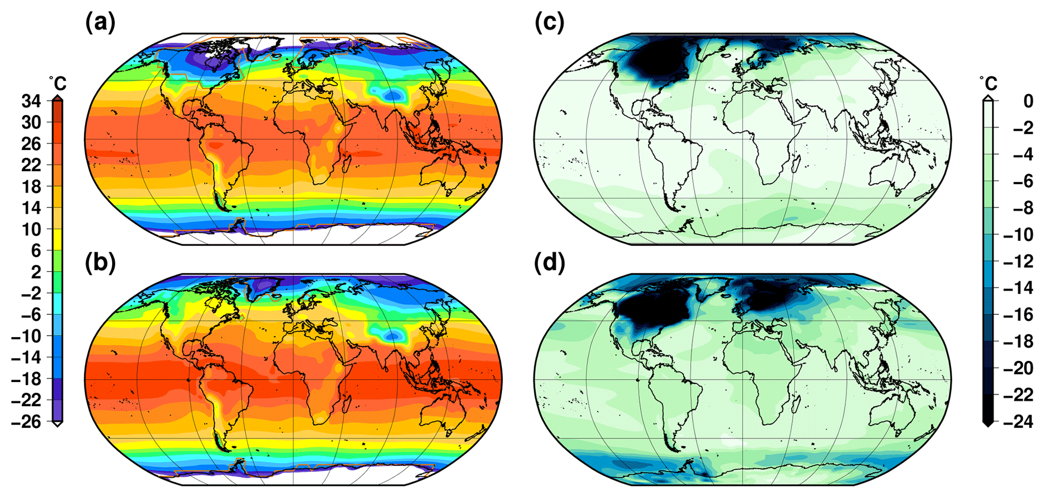
Figure 4 Simulated annual near-surface air temperature in the reference experiment DGL: (a) at the Last Glacial Maximum (21 ka) and (b) for the pre-industrial period (0 ka). (c) Simulated temperature difference between the Last Glacial Maximum and the pre-industrial period (a–b). (d) Temperature difference between the Last Glacial Maximum and the pre-industrial period in Tierney et al. (2020).

For all the experiments, we simulate a gradual warming with no abrupt climate transitions. If the different experiments show a similar temperature evolution, they also display subtle differences. First, the experiments that use a reduced freshwater flux resulting from ice sheet melting present a more rapid warming compared to the reference experiment (e.g. DGL_noFWF with respect to DGL). Second, the experiments show a diverging temperature evolution after around 13 ka. After this date, the reference DGL simulation shows a slight decrease in temperature for about 2 kyr followed by a moderate warming until ∼7 ka. By contrast, the experiment in which the freshwater fluxes are discarded (DGL_noFWF) displays a brief period during which the temperature ceases to increase followed by a sharp temperature increase. In this case, the maximal surface temperature is reached at 10 ka after which there is a slight decrease until 7 ka. DGL_FWF/3 shows a very similar temperature change as DGL_noFWF, while DGL_FWF/2 presents similarities with both DGL and DGL_noFWF. This temperature evolution is in overall agreement with the temperature reconstruction of Shakun et al. (2012), which shows a pause in the deglacial warming trends at about 13.5 ka, synchronous with the carbon dioxide plateau. The experiment with the parameterisation of brines sinking, DGL_brines, displays a comparable temperature evolution to the reference simulation DGL for most of the simulated time period. However, the brine parameterisation induces a cooling of about 0.5 ^∘C in the first years after its activation due to increased sea ice extent around Antarctica. In addition, at 4 ka, the global mean temperature starts to rise again after a relatively steady state for the rest of the Holocene. At 0 ka the temperature in the DGL_brines experiment is close to the temperature in the DGL_noFWF and DGL_FWF/3.

These differences in terms of global mean surface temperature amongst the different experiments are mostly explained by the differences in the state of the simulated Atlantic oceanic circulation. The reference experiment DGL simulates a decrease in the AMOC from the Last Glacial Maximum. After a 50 % reduction in its glacial values, the oceanic circulation strengthens at 13.5 ka for about 500 years before an abrupt collapse. This AMOC collapse is synchronous with the simulated pause in the temperature increase. From 12 ka onwards, the model simulates virtually no meridional overturning circulation. The evolution of the AMOC is drastically different when the freshwater flux to the ocean resulting from ice sheet melting is not considered (DGL_noFWF). In this case, the AMOC remains strong during the whole 26 kyr, with a maximum in the middle of the deglaciation towards 14 ka. This explains why the temperature rises more rapidly during the deglaciation in this experiment compared to the reference DGL experiment. Due to the weak AMOC in this case, the Northern Hemisphere remains colder, which ultimately delays the deglaciation of the ice sheets. The simulated pre-industrial period is also 0.8 ^∘C colder in DGL with respect to DGL_noFWF since the absence of oceanic meridional heat transport results in much colder high latitudes, especially in the North Atlantic (Fig. 5). The release of only half the meltwater flux to the ocean (DGL_FWF/2) does not allow us to maintain an active AMOC during the Holocene either, but the collapse of the AMOC is delayed here with respect to the reference experiment. In addition to the DGL_noFWF experiment, only the experiment in which only one-third of the meltwater flux is released to the ocean (DGL_FWF/3) is able to maintain an active AMOC during the Holocene. In this case, there are several abrupt oscillations in the strength of the circulation from 14 to 10 ka, but the model recovers and simulates an AMOC similar to the DGL_noFWF from 10 ka onwards. For most of the simulated time period, the experiment in which the sinking of brines around Antarctica is parameterised (DGL_brines) shows a very similar evolution than the reference DGL experiment, except that the AMOC shut-down occurs a few centuries earlier. However, at 4 ka the AMOC abruptly recovers and explains the final increase in the global mean temperature.

Figure 5 Simulated annual near-surface air temperature difference during the pre-industrial period (0 ka) from the reference experiment DGL and the experiment DGL_noFWF, in which the freshwater flux resulting from ice sheet melting is not applied to the ocean model (DGL_noFWF – DGL).

While some experiments show very abrupt shifts in the ocean, the atmospheric temperature evolution is nonetheless mostly gradual. This is visible at the global scale (Fig. 3b) but also when examining the temperature change above the Greenland ice sheet (Fig. 6a). The local temperature change closely resembles the global mean temperature change, even though with a larger amplitude. There are a few abrupt changes: slightly less than 4 ^∘C in about 200 years at 10.7 ka and at 3.8 ka for the DGL_FWF/3 and DGL_brines experiments, respectively. These are direct consequences of the AMOC recoveries visible in Fig. 3c. These simulated abrupt warming events over the Greenland ice sheet look similar to the ones of the ice core record (Fig. 6b). The North GRIP (North Greenland Ice Core Project) δ¹⁸O is generally used to reconstruct the past local temperature changes with a conversion factor of 0.67 ‰ per degree to 0.8 ‰ per degree (e.g. Johnsen et al., 1997; Buizert et al., 2014), suggesting a glacial–interglacial difference of more than 15 ^∘C. On comparable timescales, the Bølling–Allerød warming at 14.7 ka displays a similar temperature change amplitude compared to our simulated abrupt warming events, even though slightly larger. This suggests that, in our model, abrupt changes in the Atlantic oceanic circulation can induce large temperature changes over the Greenland ice sheet, similar to the ones deduced from the ice core records. However, the timing of the simulated abrupt events in the experiments shown here does not correspond to the ones of the ice record.

Figure 6 (a) Simulated surface temperature at the location of the North GRIP deep ice core. The reference model DGL is in black, while the experiments with reduced freshwater flux to the ocean from ice sheet melting are depicted with blue shading (dark blue for no freshwater flux). The experiments with enhanced brine formation are in pink. Here, we use a 10-year running mean for the model results to smooth interannual variability. (b) The isotopic content in δ¹⁸O measured at North GRIP (Andersen et al., 2004), which is often regarded as representative of local temperature changes.

3.2 Simulated ice sheet changes

The large-scale differences amongst the different experiments discussed in Sect. 3.1 are largely driven by differences in the amount of the freshwater released to the ocean related to ice sheet melting. This freshwater flux is shown in Fig. 7a for the reference experiment DGL. Even though this flux displays some variability, its evolution is generally gradual and shows a maximum around 14 ka where it peaks above 0.3 Sv (1 Sv corresponds to 10⁶ m³ s⁻¹) with 100-year mean values about 0.23 Sv. In Fig. 7a we also show the meltwater flux computed from the ice thickness changes in the ICE-6G_C and GLAC-1D geologically constrained reconstructions. These fluxes have the same order of magnitude of the simulated flux in the DGL experiment. However, the model fails to reproduce the two distinct accelerations in ice sheet retreat visible in the reconstructions for the meltwater pulse 1A at 14.6 ka (Deschamps et al., 2012) and the meltwater pulse 1B at 11.45 ka (Abdul et al., 2016). Instead, the model produces important fluxes (greater than 0.1 Sv) over a few thousand years. Another way to discuss these fluxes is to integrate them in time to have an idea of the total ice sheet volume evolution through the deglaciation (Fig. 7b). In doing so, we can see that the coupled iLOVECLIM-GRISLI model setup produces an ice volume evolution in general agreement with the reconstructions since it lies between the two estimates of ICE-6G_C and GLAC-1D most of the time. However, the coupled model seems to deglaciate too fast since it displays a lower total ice sheet volume than the two reconstructions from 12.5 ka. In Fig. 7b we also show the eustatic sea level reconstruction of Lambeck et al. (2014) which displays a larger ice sheet volume, in particular around the Last Glacial Maximum. Since we do not simulate the Antarctic ice sheet changes, the ice volume shown in this figure only represents the Northern Hemisphere ice sheet volume. Interactive simulation of the Antarctic ice sheet would result in a larger ice volume during the glacial period reducing partially the mismatch with the Lambeck et al. (2014) reconstruction. At the end of the simulation, the model has an overestimation of the present-day ice volume. This overestimation corresponds to about 4.5 m of sea level equivalent and is explained by an overestimation of the Greenland ice sheet volume and remaining small ice sheets in the Ellesmere Island, Iceland, Norway and offshore of Newfoundland (Grand Banks).

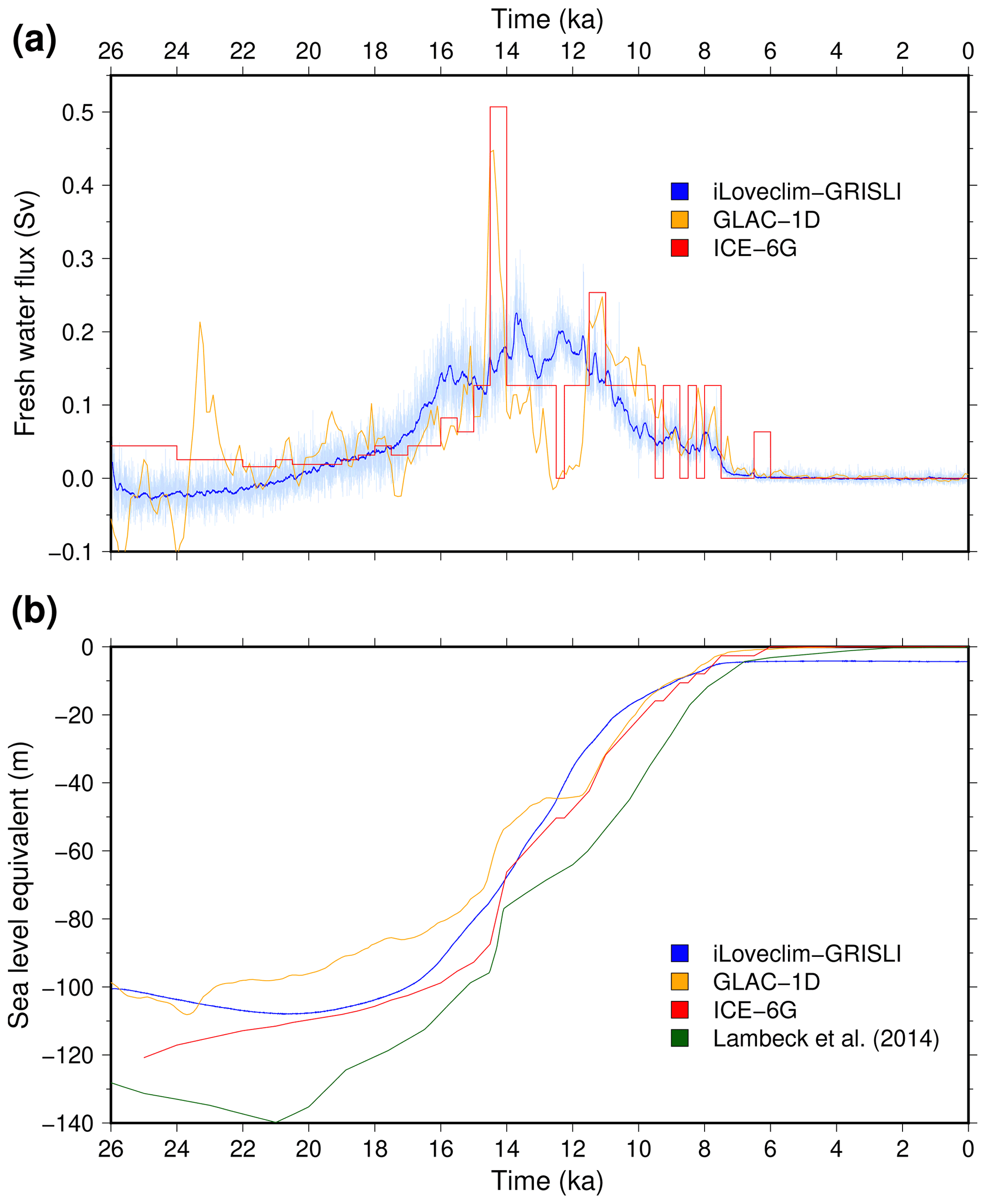
Figure 7 (a) Time evolution of the freshwater release to the ocean resulting from the computed change in the Northern Hemisphere ice sheets. The blue curve depicts the values smoothed with a 100-year running mean, while annual values are depicted in light blue. The ice mass change for the two geologically constrained reconstructions of GLAC-1D and ICE-6G_C is depicted in orange and red, respectively. (b) Corresponding eustatic sea level evolution.

The ice volume evolution of individual ice sheets is presented in Fig 8 for both the reference DGL and the DGL_noFWF experiments. In this figure, the individual ice sheet break-up is also represented for the ICE-6G_C and the GLAC-1D reconstructions. The ice volume partitioning is well reproduced. The North American ice sheet is by far the largest contributor for the last glacial sea level fall. At 26 ka, we simulate an ice volume of 81 m of sea level equivalent within the range of the geological reconstructions (75 and 86 m). However, in our experiments, the North American ice sheet volume increases until 20.5 ka where the reconstructions suggest a decline already as early as 26 ka (ICE-6G_C) or 23.8 ka (GLAC-1D). This is mostly due to our methodology used to define the initial state for the coupled experiments. When the coupling starts, at the beginning of our experiments, there is an abrupt change in the climate model in terms of ice mask and surface elevation from GLAC-1D to our spun-up ice sheets. Our spun-up ice sheets at 26 ka (Fig. 2a) show a higher North American ice sheet surface elevation than the GLAC-1D reconstruction used during the climatic spin-up, suggesting an overestimation of the precipitation in this area. When the coupling starts, this precipitation bias is amplified due to higher surface elevation and related increased orographic precipitation. The iLOVECLIM climate model likely shows an underestimation of the elevation desertification effect over the ice sheets (Quiquet et al., 2018b). The simulated volume of the Eurasian ice sheet displays a similar evolution than the North American ice sheet with a maximum around the Last Glacial Maximum. This agrees well with the GLAC-1D reconstruction. Given its smaller volume, the absolute rate of volume loss is smaller for the Eurasian ice sheet (1.3 m per millennium) compared to the one of the North American ice sheet (5.7 m per millennium). However, the Eurasian ice sheet has already lost half its volume by 14.5 ka, whereas this occurs at 12.8 ka for the North American ice sheet. The Greenland ice sheet presents only a small volume reduction of 2.6 m of sea level equivalent, in good agreement with the reconstructions. However, the Greenland ice sheet volume at the end of the simulation is largely overestimated compared to the present-day observations (about 40 % volume overestimation). As for the total volume, the individual ice sheets deglaciate faster in the DGL_noFWF experiment. This is particularly visible for the North American ice sheet for which there is a difference of 1000 years at about 11 ka.

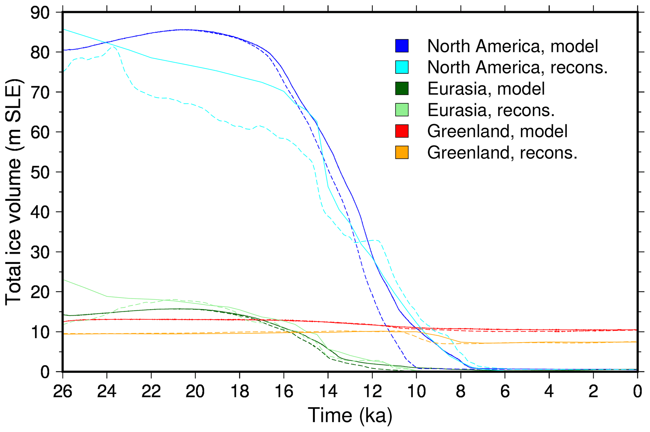
Figure 8 Individual ice sheet contributions to deglacial sea level rise, expressed as metres of sea level equivalent (SLE). For our model experiments, we show the ice volume for the reference experiment DGL (plain lines) and the experiment in which the freshwater flux resulting from ice sheet melting is not released to the ocean DGL_noFWF (dashed lines). For the reconstructions, we show the ICE-6G_C (plain lines) and the GLAC-1D (dashed lines) reconstructions.

A map of the simulated ice sheet configuration for selected snapshots is shown in Fig. 9. This figure shows the results for the reference DGL experiment, while the other synchronously coupled experiments show a similar deglacial pattern although with differences in timing. At 26 ka, the North American ice sheet presents some very active ice streams on its northern margin from east to west: the Hudson Strait ice stream, the Lancaster Sound ice stream and the Amundsen Gulf ice stream. In these regions, grounded ice velocities are greater than 500 m yr⁻¹. Elsewhere, the ice sheet does not present well-identified ice streams but the margins generally present large velocities, greater than 200 m yr⁻¹. The other ice sheets present a smaller ice flow. From 26 to 21 ka, there is only little change in the ice sheet except the Eurasian ice sheet retreat from the British Isles and the development of an ice shelf at the outlet of the Hudson Strait ice stream. The simulated topography at 21 ka (Fig. 2b) is close to the spun-up ice sheets used at 26 ka and generally remains in good agreement with the geologically constrained reconstructions. From 21 ka, we simulate a gradual ice sheet retreat for both the North American and the Eurasian ice sheets. The North American ice sheet mostly retreats in its southern continental part due to decreased surface mass balance related to the gradual warming. The deflected bedrock in this area leads to the apparition of proglacial lakes, already visible at 14 ka. Similarly, at this date, the southern flank of the Eurasian ice sheet also displays proglacial lakes. The eastern part of the Eurasian ice sheet, the Barents–Kara ice sheet, rapidly collapses due to a grounding line instability in the Kara sea. This instability is initiated at about 14.5 ka and results in a complete disintegration of the Barents–Kara ice sheet in about 1.2 ka. Such instability is favoured by the depressed bedrock, with a ∼300 m deepening in the Kara sea with respect to the present-day bathymetry, resulting in steeper retrograde slopes. Another grounding line instability occurs later for the continental part of the North American ice sheet. The grounding line retreat is clearly visible at 12 ka. This lake-induced instability considerably facilitates the North American ice sheet deglaciation (Quiquet et al., 2021a). At 8 ka, we simulate a very small North American ice sheet and only a relic of the Eurasian ice sheet over the Scandinavian mountains. At this time, the bedrock is still depressed below sea level over the northern most part of America but slowly returns to its present-day value. During the last 1000 years of the simulation, the bedrock uplift rate in the vicinity of the Hudson Bay is about 0.5 to 1.2 m per century, a value comparable to modern observations (Husson et al., 2018). The Greenland ice sheet expands considerably onto the continental shelf during the glacial period and retreats until about 10 ka. It does not display any substantial change in the ice extent during the Holocene, but it displays some ice elevation changes. The ice elevation evolution near the summit shows a maximum at about 10 ka and decreases afterwards in agreement with palaeo-elevation reconstructions at the deep ice core drilling sites (Vinther et al., 2009).

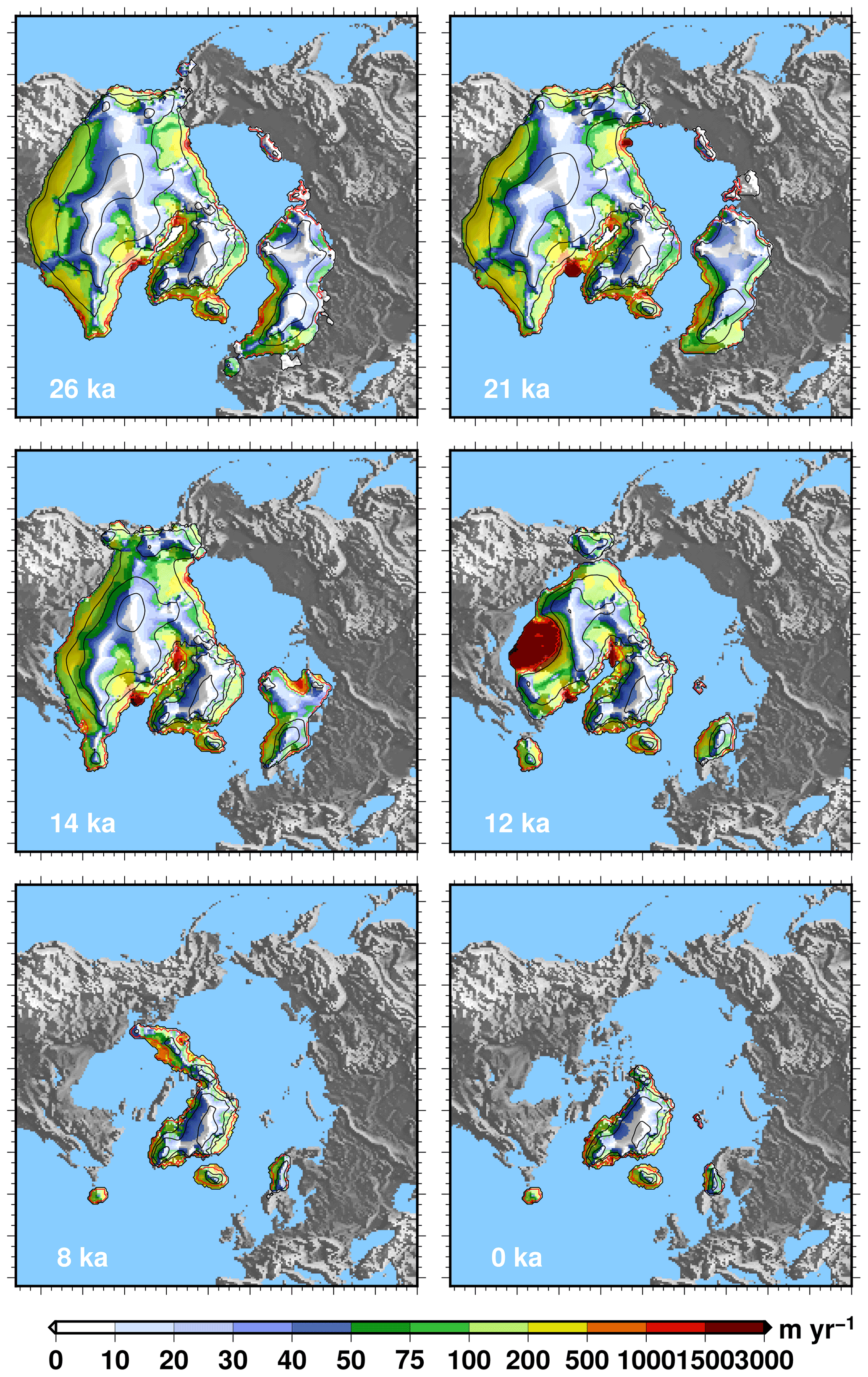
Figure 9 Simulated Northern Hemisphere ice sheets in the reference model for selected snapshots. The simulated ice elevation above contemporaneous eustatic sea level is shown with the black isocontours (separated by 1000 m). The red contour is the ice sheet grounding line. The amplitude of the simulated vertically averaged ice sheet velocity is draped over the surface topography and depicted by the colour palette. Emerged land masses are in grey, while bed elevation below contemporaneous sea level is in blue.

The chronology and pattern of the deglaciation is largely affected by the biases in the climate model. We present these biases in terms of mean annual temperature and total precipitation rate in Fig. 10. To construct this figure we use a reference pre-industrial experiment (with fixed ice sheets), performed with a similar setup to the deglaciation experiments. Notably, this pre-industrial experiment uses the same last glacial oceanic bathymetry with a closed Bering Strait. The Northern Hemisphere topography and ice mask are nonetheless at their present-day reference value for GRISLI (Amante and Eakins, 2009; Bamber et al., 2013). The model presents a cold bias associated with an overestimation of the precipitation in the northwestern part of the North American continent. This explains why this region of the North American ice sheet deglaciates much later than its eastern sector where a warm bias is present. Also, Grand Banks and Iceland remain ice covered at the end of the simulation where the model is generally too cold and too wet. More generally, the climate model tends to overestimate the precipitation over mountainous areas which can induce a positive feedback over some ice caps such as Iceland, Grand Banks, Ellesmere Island and the Scandinavian mountains.

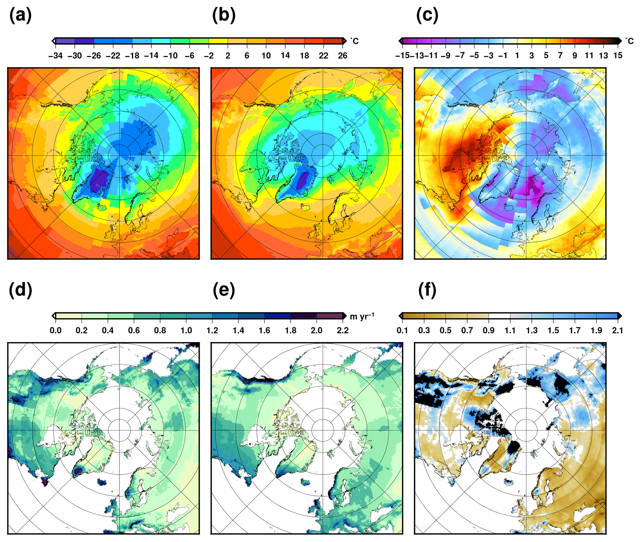
Figure 10 (a) Simulated annual near-surface air temperature for a pre-industrial climate experiment using the model configuration used for the deglaciation experiment (i.e. with an LGM ocean bathymetry) but with a present-day topography and ice mask for the Northern Hemisphere. (b) Annual near-surface air temperature for the ERA5 climatological mean over 1979–2008. (c) Temperature difference (a–b). (d) Simulated annual total precipitation rate for the same pre-industrial experiment. (e) CRU-CL-v2 annual total precipitation rate. (f) Precipitation ratio between the data in panels (d) and (e).

In Fig. 11 we present the rate of total ice mass change and its individual components: surface mass balance, basal mass balance and calving. The total mass change remains positive until 20.5 ka due to a positive integrated surface mass balance, not entirely compensated for by the basal mass loss (mostly sub-shelf melt) and calving. After this date, the total mass change becomes negative for the rest of the duration of the experiment. The total mass loss peaks at $-\mathrm{9.7}\times {\mathrm{10}}^{\mathrm{3}}$ Gt yr⁻¹ at 13.8 ka when surface ablation and loss by calving almost synchronously display a maximum (surface ablation slightly precedes the calving increase). At this date, the mass loss due to the ocean and lake represent more than half the loss by surface mass balance. In fact, if both basal mass loss and calving remain almost constant until 14.5 ka ($-\mathrm{1.4}\times {\mathrm{10}}^{\mathrm{3}}$ Gt yr⁻¹), they nonetheless show some variability after this date. These fluxes are maximal at the time of the grounding instabilities shown in Fig. 9 for both the Eurasian (14.5–13.5 ka) and the North American (12.8–10 ka) ice sheets. While the mass loss is primarily driven by surface ablation until 12.8 ka, after this date the oceanic and lake forcing become the major driver for the ice sheet retreat. The total mass loss finally reaches zero (ice sheet equilibrium) at 6.5 ka. The lesser importance of the sub-shelf melt rate for the first phase of the deglaciation could arise from the simple model we use to represent this process. Notably, we use a linear melting rate dependency on temperature change, while a quadratic dependency could best reproduce this process (Favier et al., 2019). A quadratic dependency would result in more sensitive melt rate changes to temperature changes.

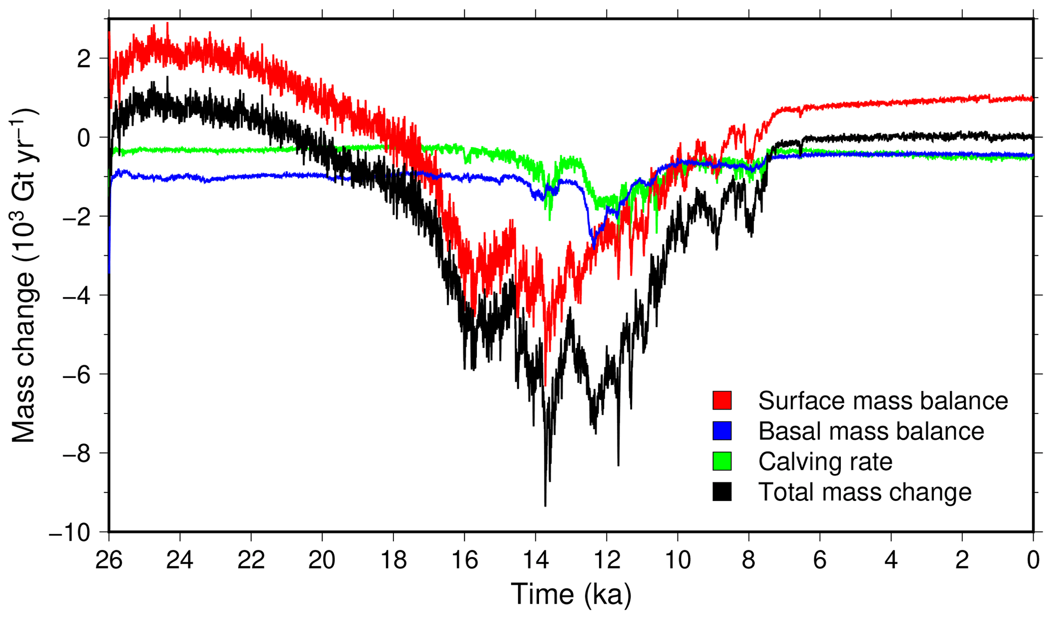
Figure 11 Time evolution of the different contributions to ice sheet mass changes. The total mass change is the sum of the surface mass balance, the basal mass balance and the calving rate.

3.3 Accelerated experiments to assess specific sensitivities

The aim of this section is to assess the sensitivity of the simulated climate evolution to the choice of critical ice sheet model parameters and assumptions. To do so, we have performed additional experiments in which the forcings are accelerated. Three major sources of uncertainties have been explored: ice sheet mechanics (deformation and grounding line dynamics), surface mass balance and sub-shelf melting rates.

The evolution of some large-scale climate variables for these additional experiments are shown in Fig. 12. Since we do not feed back the freshwater related to ice sheet melting to the ocean in the accelerated experiments, they have to be compared to the DGL_noFWF experiment. The reference accelerated experiment ADGL (black in Fig. 12) is in fact similar to the DGL_noFWF (blue): rapid temperature increase and active Atlantic circulation throughout the deglaciation. However, the accelerated experiment displays larger ice sheets than the non-accelerated (about 8 m of sea level equivalent at 14 ka) and as a result a colder climate (∼0.4 ^∘C in global mean surface temperature at 14 ka). If the timing of the ice sheet retreat can be slightly different, the overall pattern of this retreat is only weakly affected by the acceleration factor.

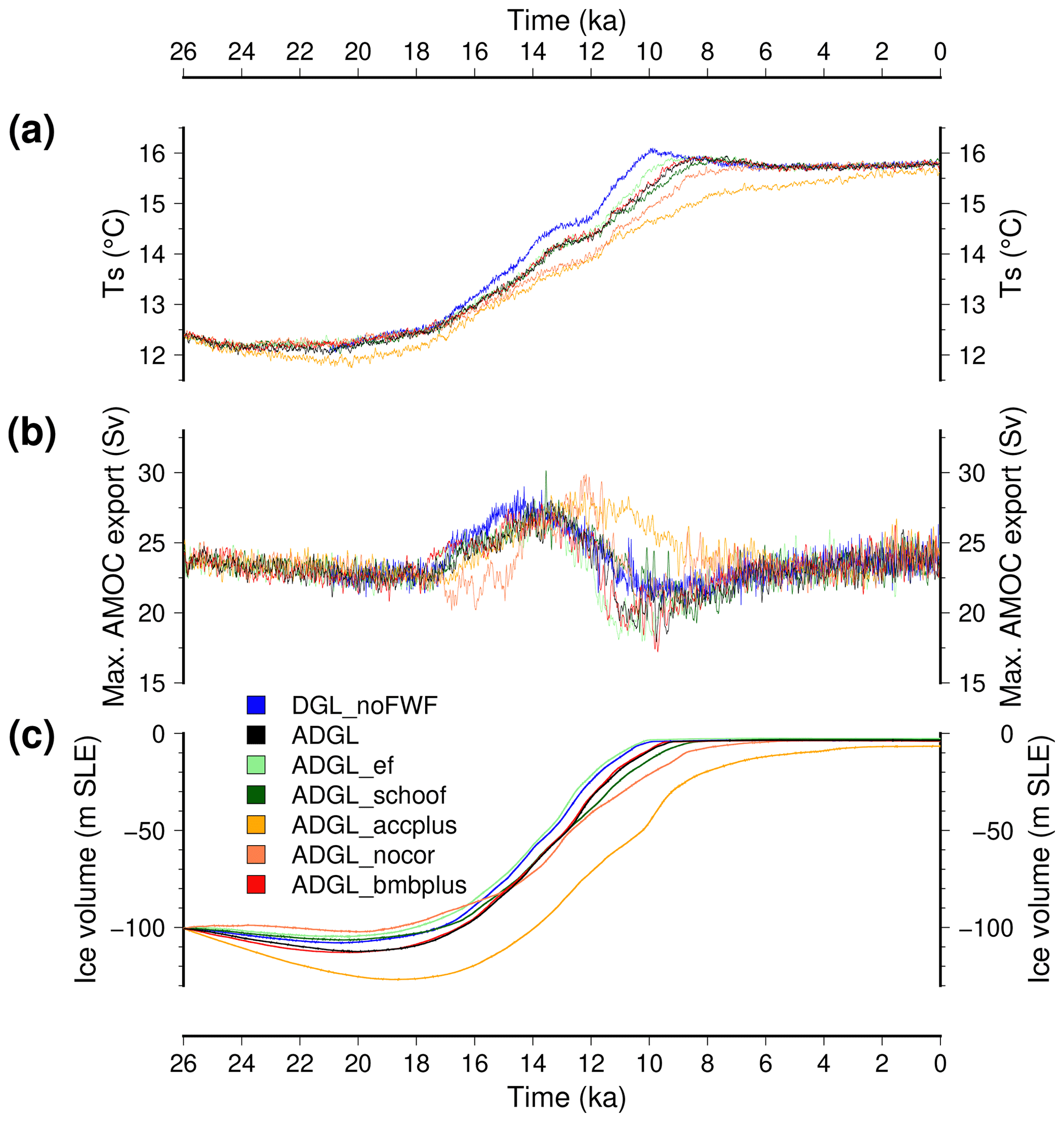
Figure 12 Time evolution of a selection of large-scale climate variables for different sensitivity experiments: (a) global mean surface temperature, (b) maximum of the Atlantic stream function and (c) simulated Northern Hemisphere ice volume. The model that does not account for the freshwater release to the ocean due to ice sheet melting is shown in grey (DGL_noFWF). The other lines are accelerated simulations (factor of acceleration of 5), and they similarly do not account for the freshwater flux to the ocean. The accelerated reference experiment is in blue (ADGL). The dark green line is an experiment in which we use the Schoof (2007) formulation of the flux at the grounding line (ADGL_schoof) instead of Tsai et al. (2015). The light green line is an experiment for which we use a larger enhancement factor (3.5 instead of 1.8, ADGL_ef). The light orange line is a version of the model with a lower c_rad coefficient (−50 instead of −40 W m⁻², ADGL_accplus) which induces a more positive surface mass balance. The dark orange is for an experiment in which we do not apply the spatial correction of the c_rad parameter (ADGL_nocor). The blue line is for an experiment with an increase in sub-shelf melting rate (ADGL_bmbplus).

The two experiments related to ice sheet dynamics (ADGL_ef and ADGL_schoof) do present some differences in their simulated ice sheet volume. The increased enhancement factor (ADGL_ef) leads to thinner ice sheets (smaller ice volume) and, as such, deglaciates faster than the reference accelerated experiment (ADGL). The experiment in which we use the formulation of Schoof (2007) instead of Tsai et al. (2015) (ADGL_schoof) also produces a lower ice sheet volume during the glacial period. However, this experiment shows a slower ice sheet retreat during the deglaciation compared to the reference ADGL experiment. This is mostly related to the greater grounding line sensitivity in the formulation of Tsai et al. (2015), already shown in (Quiquet et al., 2018a) for the Antarctic ice sheet. These differences in terms of ice sheet evolution nonetheless only have a limited impact on the climate evolution. The ADGL_ef produces a slightly more rapid warming during the deglaciation (related to the smaller ice sheets), while it is the opposite for the ADGL_schoof (slower ice sheet retreat). The Atlantic circulation is also weakly impacted by the different ice sheet evolution. Only the ADGL_ef produces a slightly earlier decrease in the overturning circulation than the ADGL experiment, while the ADGL_schoof displays insignificant differences.

The two experiments related to modification of the surface mass balance parameters induce larger simulated ice sheet volume differences. Associated with a larger ice sheet surface mass balance, the ADGL_accplus produces larger ice sheet volumes throughout the whole simulated time period. For this experiment the maximal ice volume is reached by circa 19 ka, and it is larger by about 15 m of sea level equivalent than the ADGL experiment. This excess ice also explains the delayed ice sheet retreat: at 10 ka the simulated ice sheets still represent about 45 m drop in eustatic sea level in the ADGL_accplus experiment compared to about 8 m in the ADGL experiment. This has consequences for the simulated climate: (i) the global mean temperature rises more slowly, eventually reaching a comparable value to the reference simulation at 0 ka; (ii) the phase of very active overturning in the middle of the deglaciation is extended by 2 kyr. Even though the ADGL_accplus experiment displays larger ice sheet volume, the pattern of the ice sheet retreat is similar to the one of the ADGL experiment. By contrast, the ADGL_nocor experiment provides alternative ice sheet histories. In the ADGL experiment the Barents–Kara sector of the Eurasian ice sheet is almost fully deglaciated at 13.5 ka, while it is the case only after 8.5 ka in the ADGL_nocor experiment. Conversely, the North American ice sheet retreats faster in the ADGL_nocor experiment. This is a direct consequence of the cold temperature bias in northern Europe and the warm bias in North America. If the climate evolution is not drastically changed as a result of these different ice sheet chronologies, it nonetheless shows some interesting differences. The overturning circulation remains moderate for a longer time period compared to the ADGL experiment since it increases only after 15 ka (with respect to 17.5 ka in ADGL). As a result the global mean temperature in ADGL_nocor is colder than in ADGL even though it shows smaller ice sheets at least until 15 ka. The oceanic circulation in the model seems largely affected by the Eurasian ice sheet size.

Finally, the experiment in which we increase the sub-shelf melting rate, ADGL_bmbplus, shows only negligible changes with respect to the ADGL experiment. This suggests that, in our model, the ice sheet retreat is mostly driven by surface ablation and not sub-shelf melt.

4 Discussion

We have shown that in our reference experiment the freshwater flux to the ocean resulting from ice sheet melting leads to a progressive weakening of the Atlantic overturning circulation from the Last Glacial Maximum, eventually leading to a complete shut-down without recovery within the time frame of the experiments presented. With different sensitivity experiments in which we modify the amount of freshwater flux released to the ocean, we have shown that we are able to simulate abrupt transitions from collapsed to recovered state of the Atlantic circulation during the deglaciation. Thus, with a reduced freshwater flux, the AMOC can remain active during the Holocene. This suggests that if the model contains the physical elements for rapid changes in the AMOC, it seems nonetheless too sensitive to the amount of freshwater since it is unable to maintain an active oceanic circulation with a realistic amount of freshwater fluxes. Alternative experiments (not discussed here) with the iLOVECLIM model in which we used prescribed ice sheet reconstructions (instead of interactive) and freshwater fluxes derived from the GLAC-1D and ICE-6G_C also lead to a shut-down of the overturning circulation. This problem has been identified in other models. For example, freshwater derived from geologically constrained ice sheet reconstructions (ICE-5G, Peltier, 2004) also leads to an AMOC collapse in Bethke et al. (2012), while most of the time idealised freshwater scenarios, which can substantially differ from the reconstructions, are preferred (e.g. Liu et al., 2009; Menviel et al., 2011; He et al., 2013; Obase and Abe-Ouchi, 2019). Transient sensitivity of the simulated AMOC to freshwater flux remains an open question when attempting to simulate the climate evolution across the last deglaciation. For these transient experiments, it would be useful to perform a systematic analysis of the sensitivity of the oceanic circulation to key processes for deep convection, such as the brine rejection during sea ice formation or atmospheric wind stress and also in the way the freshwater flux is imposed on the oceanic model, e.g. considering the depth of the freshwater release, its seasonality or the impact of the iceberg transport.

The simulated temperature change during the deglaciation is generally very gradual with no abrupt transitions. For example, in our experiments over the Greenland ice sheet the local temperature change is strongly correlated to the global mean temperature change and most of the time does not display abrupt events such as the one recorded in ice cores (Alley, 2000b). In fact only the abrupt AMOC recoveries in certain experiments (DGL_FWF/3 at 10.7 ka and DGL_brines at 3.8 ka) are able to produce abrupt temperature changes in Greenland comparable to the ice core record. Since these AMOC recoveries are lacking in the majority of our experiments we generally largely underestimate the millennial-scale variability observed at high latitudes. This variability could largely influence the ice sheet evolution. For example, since the Bølling–Allerød warming is not simulated in our model, we are not able to quantify its impact on the North American or the Eurasian ice sheets (Gregoire et al., 2016; Brendryen et al., 2020).

In addition, within the experiments presented here, only changes in the AMOC related to freshwater flux are able to produce some abrupt temperature changes. For example, all the accelerated experiments, in which this process is not considered, have produced a smooth temperature increase since the LGM. However, these experiments show different ice sheet evolutions with some rapid ice sheet retreat at times. This suggests that in our model and for the time period simulated, external forcing and ice sheet changes alone are not able to produce millennial-scale climate variability without invoking freshwater hosing.

Finally, we have identified a few expected improvements.

First, in our experiments we did not consider the potential changes in the Antarctic ice sheet since we use a constant topography and ice mask in the Southern Hemisphere. Similarly we do not take into account the freshwater flux resulting from Antarctic ice sheet retreat from the Last Glacial Maximum. This simplification was motivated by the fact that an earlier study already identified that freshwater hosing around Antarctica with our model has a negligible impact on the simulated climate (Roche et al., 2010). In this region, the circumpolar current tends to rapidly dilute the released freshwater leading to a very limited impact on vertical oceanic mixing. However, the gradual retreat of the ice sheet from the continental shelf margin can also facilitate the sinking of brines and as such enhance dense water formation. If the sinking of brines around Antarctica seems to play a moderate role in our experiments, it can nonetheless produce an abrupt AMOC recovery at 3.8 ka, not occurring in the reference experiment. As such, this process should be more thoroughly investigated with, for example, interactive Antarctic topography and bathymetry.

Second, we have used a very simple parameterisation for sub-shelf melt when alternative parameterisations display a better agreement with complex sub-shelf cavity oceanic models (Favier et al., 2019). This process is key for the future of Antarctic ice sheet (Seroussi et al., 2020) and could be equally important for the deglaciation of marine-based sectors of the Northern Hemisphere ice sheets (Petrini et al., 2018; Clark et al., 2020). For this reason, we plan to implement an alternative sub-shelf melt model at the interface between GRISLI and iLOVECLIM. However, in our experiments, the main driver for ice sheet retreat is surface mass balance, at least until 12.8 ka. After this date, sub-shelf melt rate becomes important only because grounding line instabilities have been triggered. These instabilities do not seem to be triggered by an artificially high grounding line melting rate since the experiment with higher sub-shelf melt displays a very similar ice sheet evolution. These results could be revisited with a more complex sub-shelf model.

Lastly, we run deglaciation experiments starting from 26 ka assuming that the Northern Hemisphere ice sheets were in equilibrium with the simulated glacial climate. However, the Last Glacial Maximum ice sheets were the results of the long previous glacial period starting from the last glacial inception. Ideally, it would have been best to perform a transient coupled experiment covering this period of time in order to have more realistic ice sheet states. Notably, slowly evolving ice sheet variables such as glacial isostasy or internal temperatures are expected to be affected by a transient spin-up instead of a constant glacial spin-up. However, it currently remains a numerical challenge to perform such a transient spin-up.

5 Conclusions

In this paper, we have presented climate model experiments in which the Northern Hemisphere ice sheets are synchronously coupled to the rest of the system (atmosphere and ocean). For the majority of our experiments, the atmospheric changes are mostly gradual, while the Atlantic overturning circulation displays abrupt changes. In the reference experiment, the model fails at keeping an active circulation during the Holocene. It is only when the freshwater amounts released to the ocean are reduced that we can simulate AMOC shut-downs and recoveries, suggesting too strong a sensitivity of this process in our model. The AMOC recoveries, when simulated, are associated with abrupt warming events in Greenland. The simulated ice sheet evolution is in general agreement with geologically reconstructions even though the retreat is too fast with respect to these reconstructions. The simulated ice sheets present some phases of acceleration in their retreat related to grounding line instabilities. These occur in the Arctic Ocean for the Eurasian ice sheet and in proglacial lakes at the southern margin of the North American ice sheet. However these events are not directly correlated to abrupt climate changes. In addition, we performed various sensitivity experiments in which we did not consider the freshwater released to the ocean but in which we modified some critical aspects of the ice sheet model. If these experiments produce different ice sheet deglacial chronologies they show similar climate trajectories. This suggests that ice sheet geometry changes alone, i.e without freshwater fluxes, are not enough to generate abrupt events in our model.