PMIP4/CMIP6 last interglacial simulations using three different versions of MIROC: importance of vegetation

We carry out three sets of last interglacial (LIG) experiments, named lig127k, and of pre-industrial experiments, named piControl, both as part of PMIP4/CMIP6 using three versions of the MIROC model: MIROC4m, MIROC4m-LPJ, and MIROC-ES2L. The results are compared with reconstructions from climate proxy data. All models show summer warming over northern high-latitude land, reflecting the differences between the distributions of the LIG and present-day solar irradiance. Globally averaged temperature changes are −0.94 K (MIROC4m), −0.39 K (MIROC4m-LPJ), and −0.43 K (MIROC-ES2L). Only MIROC4m-LPJ, which includes dynamical vegetation feedback from the change in vegetation distribution, shows annual mean warming signals at northern high latitudes, as indicated by proxy data. In contrast, the latest Earth system model (ESM) of MIROC, MIROC-ES2L, which considers only a partial vegetation effect through the leaf area index, shows no change or even annual cooling over large parts of the Northern Hemisphere. Results from the series of experiments show that the inclusion of full vegetation feedback is necessary for the reproduction of the strong annual warming over land at northern high latitudes. The LIG experimental results show that the warming predicted by models is still underestimated, even with dynamical vegetation, compared to reconstructions from proxy data, suggesting that further investigation and improvement to the climate feedback mechanism are needed.

1 Introduction

The last interglacial (LIG, 130–116 ka) is referred to as the warmest period in the recent glacial–interglacial cycle (NGRIP members, 2004; Overpeck et al., 2006; Lang and Wolff, 2011). The most important characteristic of the LIG is the strong summer solar irradiance in the Northern Hemisphere due to the difference between the Earth's orbit during that period and that of the present day (Berger, 1978; Yin and Berger, 2015). For example, 127 000 years ago, the peak summer solar irradiance was more than 70 W m⁻² larger compared to that of the present day at 65^∘ N (Fig. 1). Geological evidence shows that the globally averaged temperature was higher by 1.9 K in the LIG compared to the pre-industrial (Turney and Jones, 2010). The sea surface temperature (SST) also shows a warming of 0.7 ± 0.6 K (McKay et al., 2011) and 0.5 ± 0.3 K (Hoffman et al., 2017). Records from ice cores show warming in Greenland (NEEM, 2013; Masson-Delmotte et al., 2011) and in Antarctica (Jouzel et al., 2007; Stenni et al., 2010; Capron et al., 2017). Sea level rise due to warming has also been pointed out, with contributions from the mass balance change in the Greenland and Antarctic ice sheets. The total sea level rise in the LIG is estimated to be 5.5–9.0 m (Dutton and Lambeck, 2012; Dutton et al., 2015). The contribution from the Greenland ice sheet is estimated to be 1.4–4.3 m (Robinson et al., 2011; Born and Nisancioglu, 2012; Quiquet et al., 2013; IPCC, 2013), 2–4 m (Dutton and Lambeck, 2012), and 0.6–3.5 m (Stone et al., 2013). Paleo-evidence shows substantial summer warming at northern high-latitude land areas (typically +4–5 K, at most +8 K) in response to this different spatial and temporal pattern of solar irradiance (CLIP members, 2006; Otto-Bliesner et al., 2006; Velichko et al., 2008). A northward shift of the boreal treeline due to warming is also indicated by proxies (LIGA members, 1991; Edwards et al., 2003). In the Sahara, vegetation is estimated to be expanded northward due to wetter conditions (Larrasoaña et al., 2013).

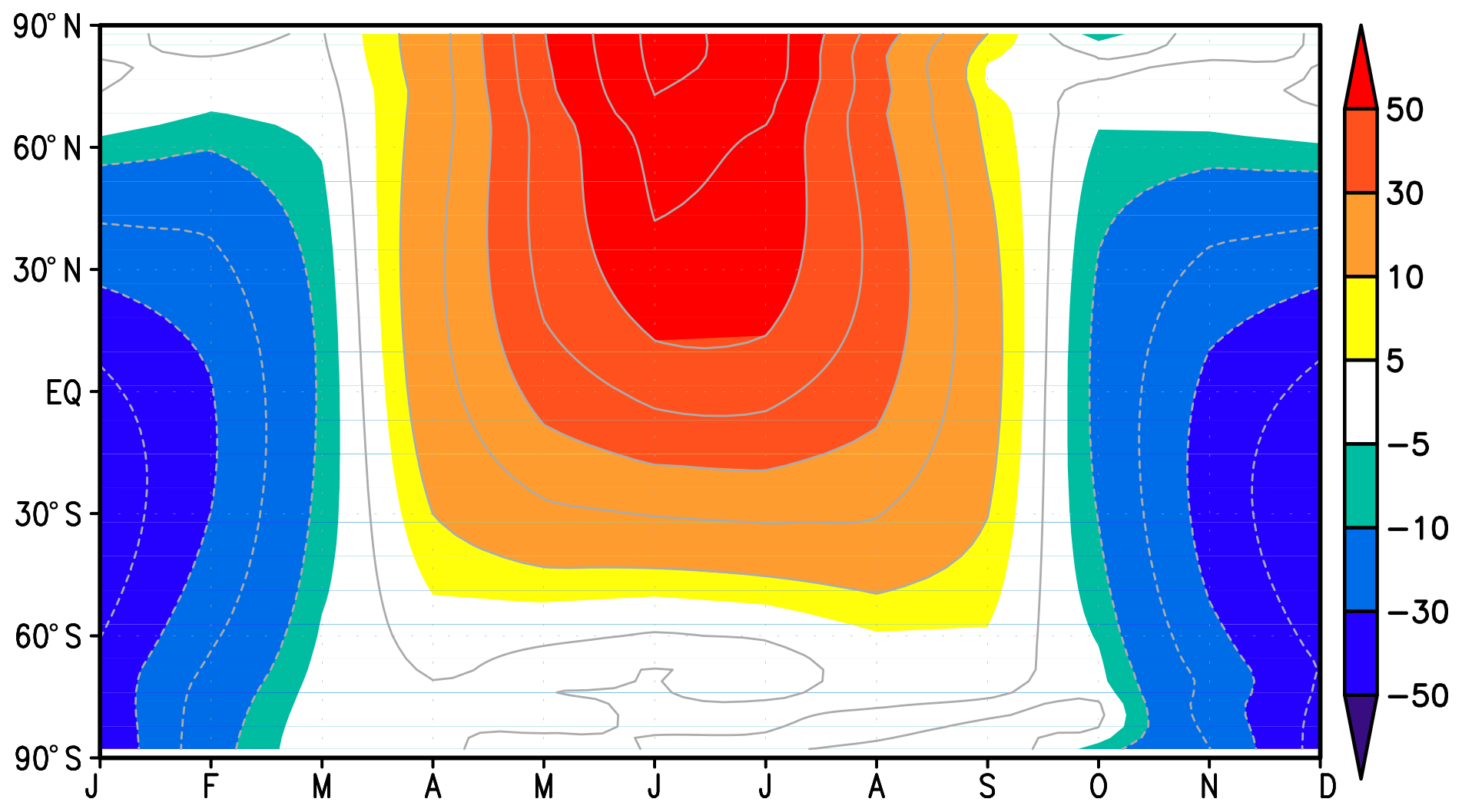
Figure 1 Latitude–month insolation anomaly between 127k and PI (W m⁻²). The calendar for 127k is adjusted using a method based on Bartlein and Shafer (2019).

The Paleoclimate Modelling Intercomparison Project (PMIP) coordinates the cooperation and comparison between modeling and data for the past (Braconnot et al., 2000, 2007, 2012; Kageyama et al., 2018). The LIG is one of the targeted periods in addition to the mid-Holocene and the Last Glacial Maximum (Lunt et al., 2013; Otto-Bliesner et al., 2017). For the simulation of past periods, PMIP provides protocols with common settings that should be applied to participating models. In the present study, we apply the LIG boundary conditions provided by the PMIP4 to three different versions of atmosphere–ocean coupled general circulation models (AOGCMs), which belong to the Model for Interdisciplinary Research on Climate (MIROC) family, and compare results with the pre-industrial simulations, focusing on the different treatment of vegetation among the three models. In Sect. 2, models and their components are described. The experimental settings are also mentioned in Sect. 2. Section 3 describes the results of LIG model simulations and comparison with proxies. In Sect. 4, we discuss the validity of data–model comparison. The feedback mechanism for the Arctic warming amplification is also discussed.

2 Models and settings

2.1 Models

In this section, the models used in the present study, MIROC4m, MIROC4m-LPJ, and MIROC-ES2L, are described. An overview of the models is shown in Fig. 2. Their critical difference among others is that MIROC4m prescribes a modern vegetation distribution with corresponding leaf area indices, MIROC-ES2L prescribes modern vegetation distribution but allows leaf area indices to respond to the simulated climate, and MIROC4m-LPJ simulates both vegetation distribution and leaf area indices in response to climate change. Therefore, comparisons of these three models provide an opportunity to loosely reveal the effect of no, partial, and full vegetation feedbacks. We note, however, that the effect of other differences in model resolution and physics cannot be excluded. MIROC4m and MIROC-LPJ do not include a carbon feedback upon the climate. MIROC4m-LPJ predicts changes in land surface properties depending on vegetation change. MIROC-ES2L includes the prediction of atmospheric carbon and nitrogen content as greenhouse gases (GHGs), but the radiative effect of GHGs is fixed in the present study (see settings).

Figure 2 Schematic of models.

2.1.1 MIROC4m

The AOGCM, MIROC4m, is based on MIROC3.2, which contributed to the fourth assessment report (AR4; Meehl et al., 2007) of the Intergovernmental Panel on Climate Change (IPCC). MIROC4m consists of the Center for Climate System Research Atmosphere General Circulation Model (CCSR AGCM; Hasumi and Emori, 2004) and the CCSR Ocean Component Model (COCO; Hasumi, 2006). The AGCM solves the primitive equations on a sphere using a spectral method (Numaguti et al., 1997). The model resolution of the atmosphere component is T42 with 20 vertical layers. The land submodel is the Minimal Advanced Treatments of Surface Interaction and Runoff (MATSIRO; Takata et al., 2003). Vegetation is prescribed as a satellite-based present-day distribution. The OGCM solves the primitive equation on a sphere, whereby the Boussinesq and hydrostatic approximations are adopted (Hasumi, 2006). The horizontal resolution is ∼ 1.4^∘ in longitude and 0.56–1.4^∘ in latitude (latitudinal resolution is finer near the Equator), and there are 43 vertical layers. The OGCM is coupled to a dynamic–thermodynamic sea ice model (Hasumi, 2006). MIROC4m has been used extensively for modern climate (Obase et al., 2017), paleoclimate (Ohgaito and Abe-Ouchi, 2007; Abe-Ouchi et al., 2013; Sherriff-Tadano et al., 2018), and future climate studies (Yamamoto et al., 2015).

2.1.2 MIROC4m-LPJ

We recently developed a vegetation coupled AOGCM MIROC4m-LPJ by introducing the Lund–Potsdam–Jena Dynamical Global Vegetation Model (LPJ-DGVM; Sitch et al., 2003) into MIROC4m. The coupling method is similar to that used for MIROC-LPJ in previous studies (O'ishi and Abe-Ouchi, 2009, 2011, 2013), which adopted a motionless “slab” ocean instead of the dynamical ocean model COCO. What is new in the present study is that bias correction is not applied to the coupling between atmosphere and vegetation components. LPJ-DGVM predicts the potential vegetation distribution, which is translated to the classification used for MATSIRO annually by using monthly mean temperature, precipitation, and cloud cover predicted by the atmosphere component of the GCM. LPJ-DGVM predicts the vegetation distribution based on carbon balance, but MIROC-LPJ does not include a carbon cycle or its feedback to the climate. Leaf area index (LAI) seasonality in MIROC-LPJ is prescribed with a sine curve, which is defined by maximum and minimum values for each vegetation type. A detailed description of the method can be found in O'ishi and Abe-Ouchi (2009). Another important modification is the introduction of a wetland scheme developed by Nitta et al. (2017). This scheme improves the seasonality of the hydrological behavior over land. When snowmelt occurs, some of the meltwater does not immediately discharge into rivers but remains in isolated storage. This stored water decays with a timescale dependent on the standard deviation of the topography, and the amount of decayed water is taken into account in the land surface water and energy balance. The introduction of this scheme reduces the summer warm bias over land at middle to high latitudes. The model resolutions of the atmosphere and land are the same as those of MIROC4m. The resolution of LPJ-DGVM is T42.

2.1.3 MIROC-ES2L

An Earth system model (ESM), the MIROC Earth System version 2 for long-term simulations (MIROC-ES2L; Hajima et al., 2020; Ohgaito et al., 2020), is one of the contributing models to PMIP4/CMIP6. The physical component of MIROC-ES2L is MIROC5.2 (Tatebe et al., 2018), an upgraded version of MIROC5 (Watanabe et al., 2010), which contributed to the IPCC AR5 (IPCC, 2013). In MIROC-ES2L, the sea ice component is updated from MIROC4m to a sub-grid multicategory model described in Komuro and Suzuki (2013). The most important update in MIROC-ES2L from previous versions of MIROC-ESM (Watanabe et al., 2011; Kawamiya et al., 2005) is the introduction of a nitrogen cycle. The land nitrogen and carbon cycles are predicted by a modified version of the Vegetation Integrative Simulator for a Trace gas model, VISIT (Ito and Inatomi, 2012), referred to hereafter as VISIT-e. The vegetation distribution is prescribed in both MATSIRO and VISIT-e, but the LAI is predicted daily by VISIT-e and transferred to MATSIRO. The ocean nitrogen and carbon cycles are predicted by an ocean biogeochemical component model, OECO₂. Detailed information is described in Hajima et al. (2020) and Ohgaito et al. (2020). The model resolution of the atmosphere component is T42 with 40 vertical layers. The model resolution of the ocean component is a warped tripolar coordinate system with longitudinal 1^∘ grid spacing in the spherical coordinate south of 63^∘ N and meridional grid spacing varying from 0.5^∘ (near the Equator) to 1^∘ (midlatitudes). The number of vertical layers is set to 63.

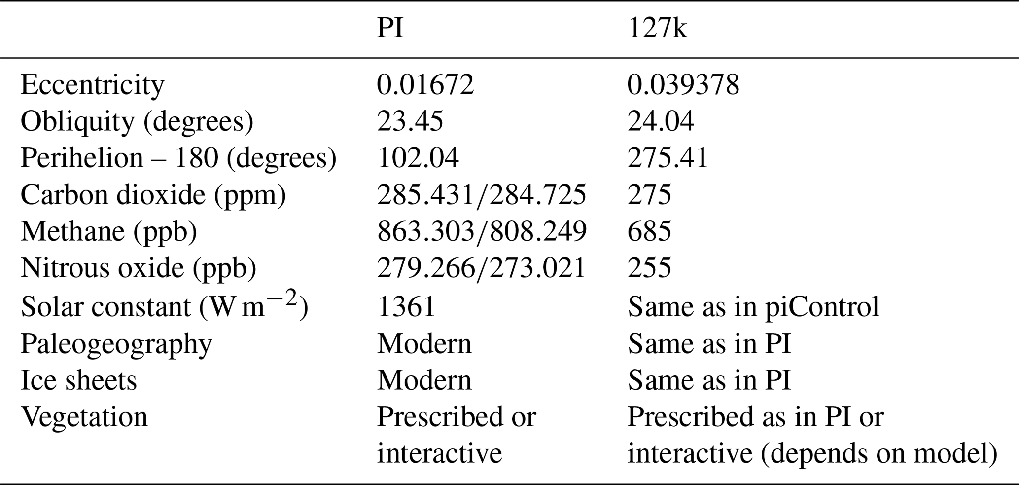
Table 1 Forcings and boundary conditions of the pre-industrial (PI) and last interglacial (127k). Greenhouse gas levels for MIROC-ES2L are shown in the PI column.

2.2 Settings

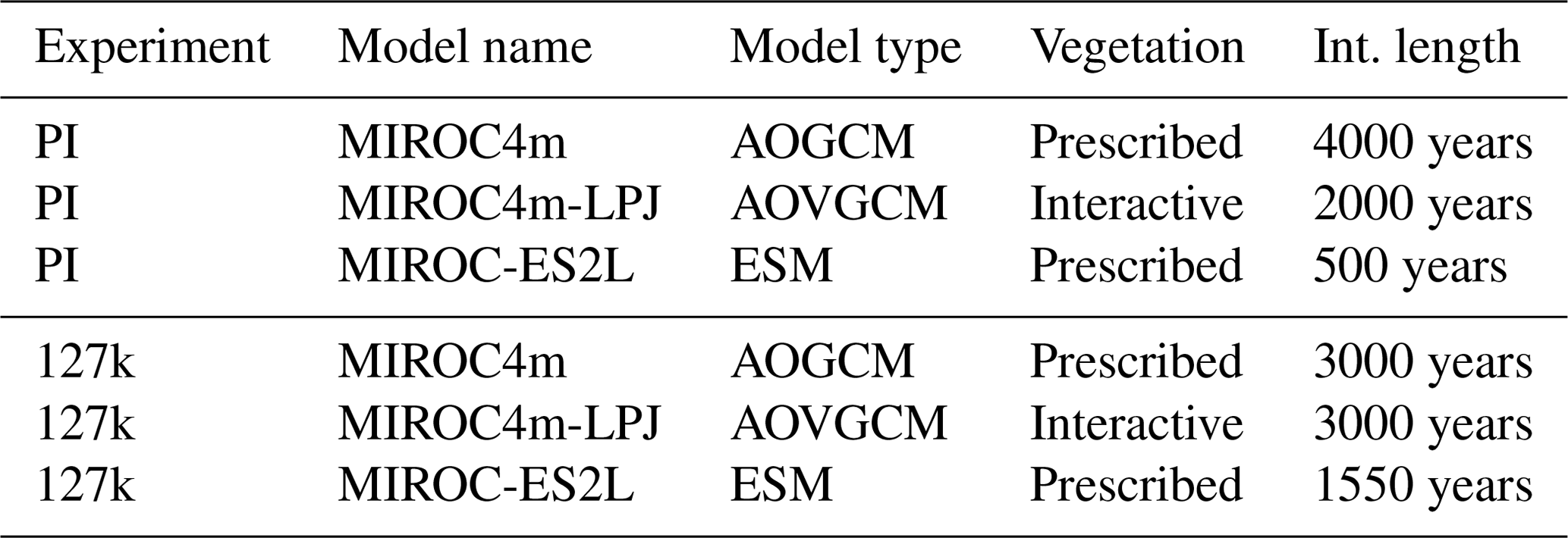
In the present study, three models are run with the same forcings and with the boundary conditions of the pre-industrial (piControl in PMIP4/CMIP6, hereafter PI) and of the last interglacial (lig127k in PMIP4, hereafter 127k), as shown in Table 1, following the PMIP4/CMIP6 protocol (Otto-Bliesner et al., 2017). The orbital forcings in both experiments are the same as those recommended in Otto-Bliesner et al. (2017). The GHG concentrations in piControl are slightly different from Otto-Bliesner et al. (2017). We apply fixed GHG values from the CMIP3 control experiment to MIROC4m and MIROC4m-LPJ. In MIROC-ES2L, GHGs are fixed to the same as the CMIP6 DECK piControl experiment settings. The GHG concentrations in the 127k experiments are fixed to the same as those specified in Otto-Bliesner et al. (2017) in all GCMs. Details on these GHG values are shown in Table 1. Especially in MIROC-ES2L, the carbon balance in the land and ocean ecosystem does not affect the atmospheric CO₂ concentration in the present study. Paleogeography and ice sheets are set to modern in all experiments. The vegetation distribution in MIROC4m is fixed to the present-day configuration according to Ramankutty and Foley (1999); see Fig. 3. In MIROC4m-LPJ, the vegetation distribution is predicted as in MIROC-LPJ (O'ishi and Abe-Ouchi, 2009). MIROC-ES2L applies a new definition of the land–sea mask, different to that of MIROC4m. The distribution of prescribed vegetation is also updated from MIROC4m and redefined by using newer satellite data sets. In MIROC-ES2L, the vegetation distribution is fixed to a satellite-based vegetation distribution (Matthews, 1983, 1984; Hall et al., 2006), the same as that in MATSIRO of MIROC5 (Watanabe et al., 2010; see Fig. 2) and in the DECK piControl experiment (Hajima et al., 2020; Ohgaito et al., 2020), using VISIT-e. However, as described above, VISIT-e predicts the LAI, which is accessed by MATSIRO. In PI experiments, MIROC4m, MIROC4m-LPJ, and MIROC-ES2L are integrated for 4000 years, 2000 years, and 500 years, respectively. In 127k experiments, MIROC4m, MIROC4m-LPJ, and MIROC-ES2L are integrated for 3000 years, 3000 years, and 1550 years, respectively (Table 2). In all experiments, the last 100 years, during which the climate has reached equilibrium, are used for analysis. Since the definition of the length of months is set to the present-day calendar, monthly averaged values may not correspond exactly to the appropriate seasons at 127 ka. We applied a calendar adjustment to all 127k results based on Bartlein and Shafer (2019). Their method defines the length of months based on the arc of the Earth's orbit, which is traverse.

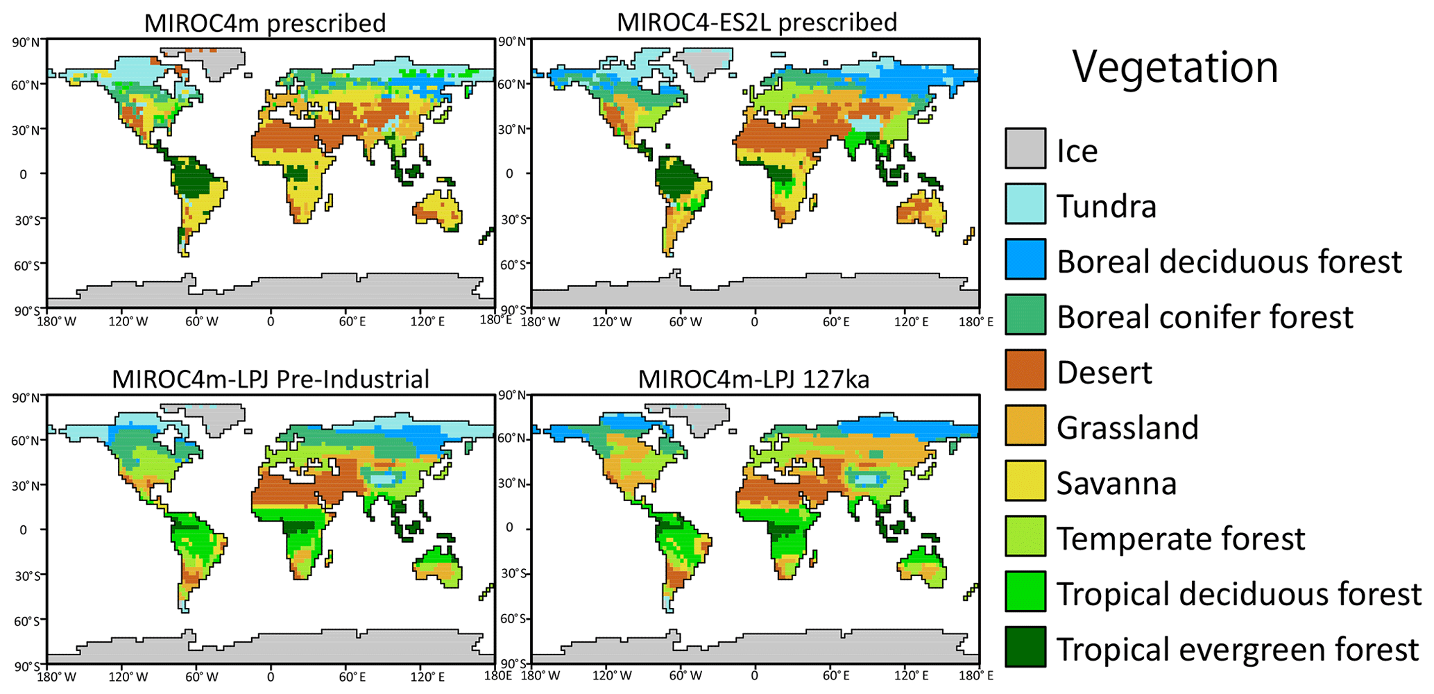
Figure 3 Vegetation distribution as a fixed boundary condition (MIROC4m and MIROC-ES2L) and the resultant most dominant vegetation types in MIROC4m-LPJ experiments in PI and 127k.

Table 2 List of experiments.

3 Results

3.1 Temperature

A look at the globally averaged annual mean temperature changes in the present study shows that there is a slight cooling from PI for all three models: −0.94 K (MIROC4m), −0.39 K (MIROC4m-LPJ), and −0.43 K (MIROC-ES2L). Seasonally and annually averaged surface air temperature differences between 127k and PI are shown in Fig. 4. All models show the largest regional warming (> 6 K) in June–July–August (JJA) over northern high-latitude land and the largest global cooling in December–January–February (DJF), which corresponds to increased boreal summer solar irradiance and decreased boreal winter solar irradiance in the LIG, respectively. In September–October–November (SON), there is still a slight warming over Northern Hemisphere land at middle and high latitudes carried over from the summer. In March–April–May (MAM), the global cooling is less than that in DJF and warming is seen at northern high latitudes. Antarctica in all models shows cooling in DJF, reflecting the decrease in solar irradiance at SH high latitudes in winter (Fig. 1).

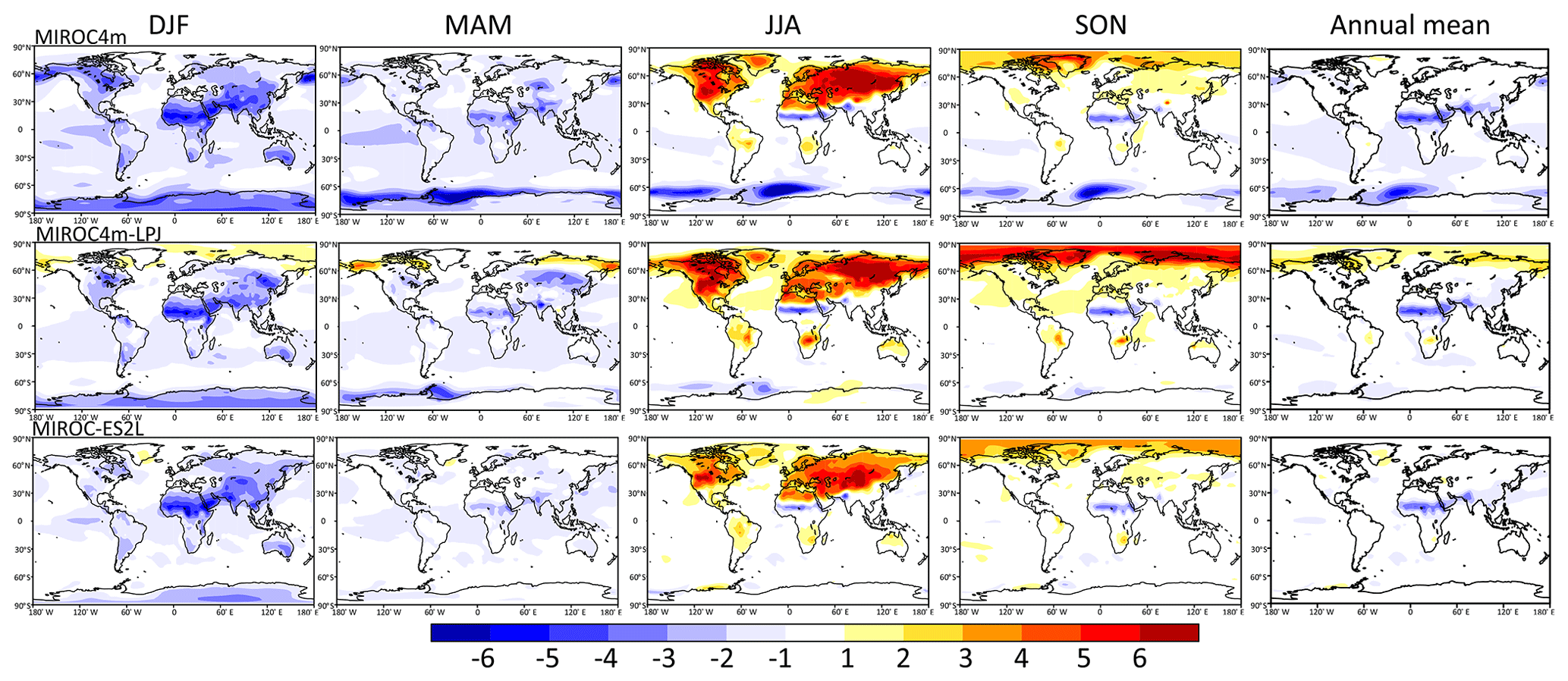
Figure 4 Seasonal and annual surface air temperature difference (K) between 127k and PI in three models. The calendar for 127k is adjusted using a method based on Bartlein and Shafer (2019).

The change in annually averaged surface air temperature is smaller than that of the seasonally averaged value because summer warming is compensated for by cooling in other seasons. MIROC4m shows global cooling except for some isolated areas where annual temperatures are higher, e.g., Greenland. MIROC4m-LPJ shows annual warming (at most 3 K) over both high-latitude land and in the Arctic Ocean, with vegetation changing from tundra to boreal forest in the northern coastal areas of Eurasia and North America (Fig. 3). Only MIROC4m-LPJ shows strong warming in Alaska and eastern Siberia, especially in MAM. The Arctic Ocean shows warming throughout all seasons in MIROC4m-LPJ, which is not seen in MIROC4m and MIROC-ES2L. MIROC-ES2L and MIROC4m-LPJ show annual warming in the Arctic Ocean, but the intensity in the former model is less. MIROC-ES2L shows annual warming in Antarctica, which is not seen in the other two models.

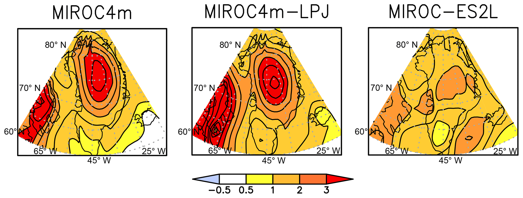
Figure 5 May–June–July–August averaged temperature difference (K) between 127k and PI in three models. The calendar for 127k is adjusted using a method based on Bartlein and Shafer (2019).

The May–June–July–August (MJJA) averaged temperature difference is shown in Fig. 5, which focuses on Greenland because the ice sheet mass balance is affected by the increased solar irradiance during MJJA at northern high latitudes (Fig. 1). MIROC4m and MIROC4m-LPJ show a similar pattern of warming that increases with altitude. MIROC-ES2L shows a more homogeneous warming pattern over Greenland, and the intensity of warming is weaker than in the other two models.

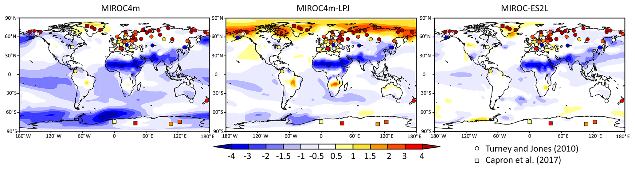
Figure 6 The annual surface air temperature change (K) between 127k and PI is compared with reconstructions by Turney and Jones (2010) and Capron et al. (2017).

Simulated temperature changes are compared with reconstructed values from proxies. In Fig. 6, annual surface temperature change is compared with land proxies by Turney and Jones (2010), hereafter referred to as TJ2010. MIROC4m-LPJ exhibits the largest warming among the three models at northern high latitudes. However, the agreement with TJ2010 is not quantitative but more qualitative; annual warming is still underestimated. The other two models show cooling over northern high-latitude land. Greenland warming appears in all models but is smaller than that of TJ2010. In Antarctica, MIROC-ES2L shows the same sign of temperature change as in TJ2010, but the intensity of warming (at most 1 K) is weaker than that of TJ2010. MIROC4m and MIROC4m-LPJ show cooling rather than warming in Antarctica. In Fig. 6, annual surface temperature change is also compared with a newer reconstruction by Capron et al. (2017), hereafter referred to as C2017. All models show warming in Greenland, but only MIROC-ES2L reproduces Antarctica warming. The models underestimate warming at all sites in C2017 as the intensity is not reproduced.

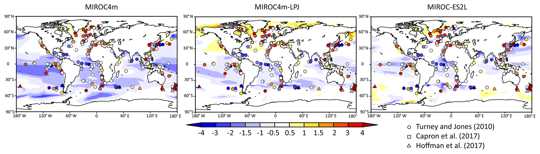
Figure 7 The annual sea surface temperature change (K) in 127k from PI is compared with reconstructions by Turney and Jones (2010), Capron et al. (2017), and Hoffman et al. (2017).

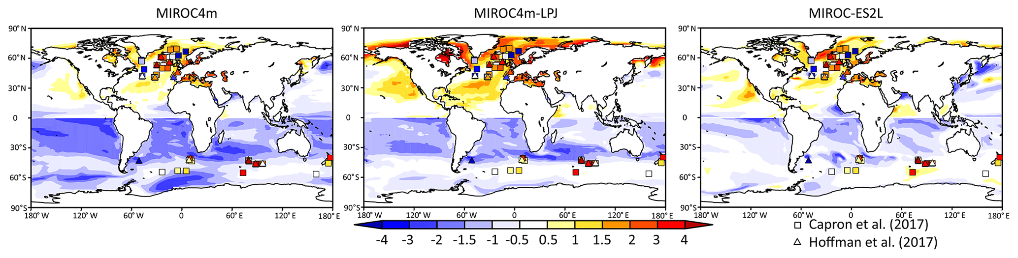
Figure 8 The summer (JJA in NH, DJF in SH) sea surface temperature change (K) in 127k from PI is compared with reconstructions by Capron et al. (2017) and Hoffman et al. (2017). The calendar for 127k is adjusted using a method based on Bartlein and Shafer (2019).

Figure 7 compares the simulated annual sea surface temperature (SST) change and TJ2010 ocean proxies. All three models predict warm SST at northern high latitudes and cooling in tropical regions. This large-scale latitudinal pattern agrees with TJ2010, but some individual sites disagree in terms of sign. For example, the NH SST warming is more substantial in MIROC4m-LPJ and in MIROC-ES2L than in MIROC4m. The largest warming in the SH is seen in MIROC-ES2L. However, the intensity of SST changes in all models is far smaller than that of TJ2010. We also compare the modeled annual SST difference with newer reconstructions by C2017 and Hoffman et al. (2017), hereafter referred to as H2017, in Fig. 7. MIROC4m underestimates warming in the Irminger Sea and shows changes of opposite sign in the southern part of the Pacific and Indian Ocean. MIROC4m-LPJ shows larger NH warming than MIROC4m. However, as with MIROC4m, warming in the SH is not simulated. MIROC-ES2L predicts better warming in the Irminger Sea than MIROC4m/MIROC4m-LPJ. MIROC-ES2L also predicts improved warming in the SH, which is partially consistent with proxies. Summer temperature changes in the models are compared with that of reconstructions by C2017 and H2017 in Fig. 8. Across the wide expanse of the northern Atlantic Ocean, all models predict warming with a sign consistent with those of reconstructions, except at some sites that show cooling. MIROC4m-LPJ predicts the largest warming (at most > 4 K), while the other two models show a smaller intensity of warming (at most 3 K) in the northern Atlantic Ocean. On the other hand, in the SH, MIROC4m and MIROC4m-LPJ show cooling in contrast to the warming indicated by proxies. MIROC-ES2L shows warming across much of the Southern Ocean, in contrast to the other two models. However, some sites still indicate an opposite sign to that of proxies.

3.2 Precipitation, sea ice, and vegetation

3.2.1 Precipitation

The precipitation change between 127k and PI is shown in Fig. 9. In general, the annually averaged precipitation changes seen in all three models are similar and show the largest increase, 700 mm yr⁻¹, at the southern edge of the Sahara. The second largest increase over land is seen in the northern part of India. The largest precipitation increase over ocean is seen in the Somali Sea. On the other hand, a precipitation decrease is mainly seen in the Southern Hemisphere. South America, South Africa, and the northern part of Australia become drier than PI. These characteristics in the model result are consistent with previous studies (Scussolini et al., 2019), except for the slight annual precipitation increase in eastern Siberia and Alaska. In our three MIROC versions, precipitation increase in eastern Siberia and Alaska is only seen in JJA. MIROC4m and MIROC4m-LPJ show almost the same precipitation change since they share the same atmosphere component. MIROC-ES2L shows a pattern slightly different to that of the MIROC4m models.

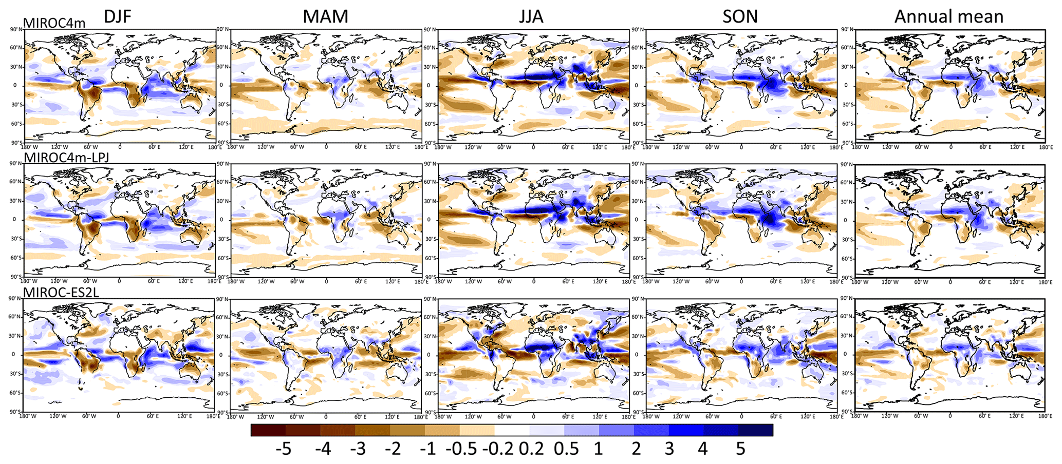
Figure 9 The annual and seasonal precipitation change (mm d⁻¹) in 127k from PI is shown. The calendar for 127k is adjusted using a method based on Bartlein and Shafer (2019).

3.2.2 Sea ice

In Fig. 10, the March NH sea ice concentration in PI and 127k, along with their difference (127k–PI), is shown for all three models. The PI sea ice distribution shows characteristics common to both MIROC4m and MIROC4m-LPJ. In PI, they show values larger than observations in the Labrador Sea, the Irminger Sea, and the Beaufort Sea. MIROC-ES2L shows a pattern different to the two MIROC4m models. The sea ice concentration in MIROC-ES2L is more realistic than MIROC4m and MIROC4m-LPJ. This is due to the different ocean and sea ice model adopted in the physical part of MIROC-ES2L. However, the sea ice concentrations in 127k and PI during March do not show any clear differences. Figure 11 shows the September NH sea ice concentration. As in March, MIROC-ES2L shows a different distribution of sea ice and response in 127k compared to MIROC4m-based models. MIROC4m-LPJ shows the largest reduction in sea ice from PI and 127k, which corresponds to a warm Arctic Ocean during those two periods. As such, MIROC4m-LPJ predicts less sea ice in September in PI compared to observations (e.g., HadISST averaged over 1870–1919; Rayner et al., 2003). The March SH sea ice concentration is shown in Fig. 12. In the Southern Ocean, all models show the sea ice extent in PI to be smaller than observations. March sea ice shows the same characteristics in the two MIROC4m-based models. MIROC-ES2L shows a different pattern, and the smallest amount of sea ice, compared with MIROC4m-based models. In all three models, March sea ice increases in 127k but the amount differs depending on the model, similar to September NH. The September SH sea ice concentration is shown in Fig. 13. As in March, there is a discrepancy between the sea ice concentrations in the MIROC4m-based models and in MIROC-ES2L. Sea ice in the PI is smaller in MIROC-ES2L and the response of sea ice in 127k is also the smallest in that model. MIROC-ES2L clearly underestimates sea ice in both seasons compared to observations.

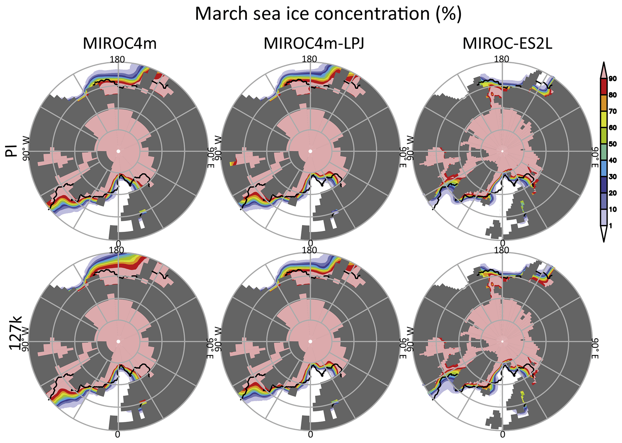
Figure 10 The NH March sea ice concentration (%) in PI and 127k, along with the difference between 127k and PI, is shown for three models. Thick lines indicate a concentration of 15 % in the climatology (the HadISST data averaged over 1870–1919). The calendar for 127k is adjusted using a method based on Bartlein and Shafer (2019).

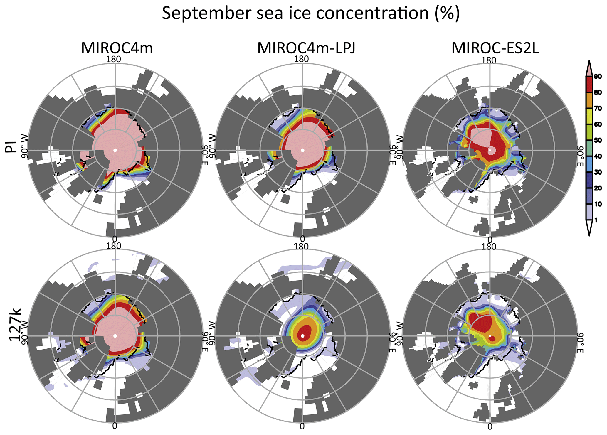
Figure 11 Same as Fig. 10 but for NH September sea ice concentration (%).

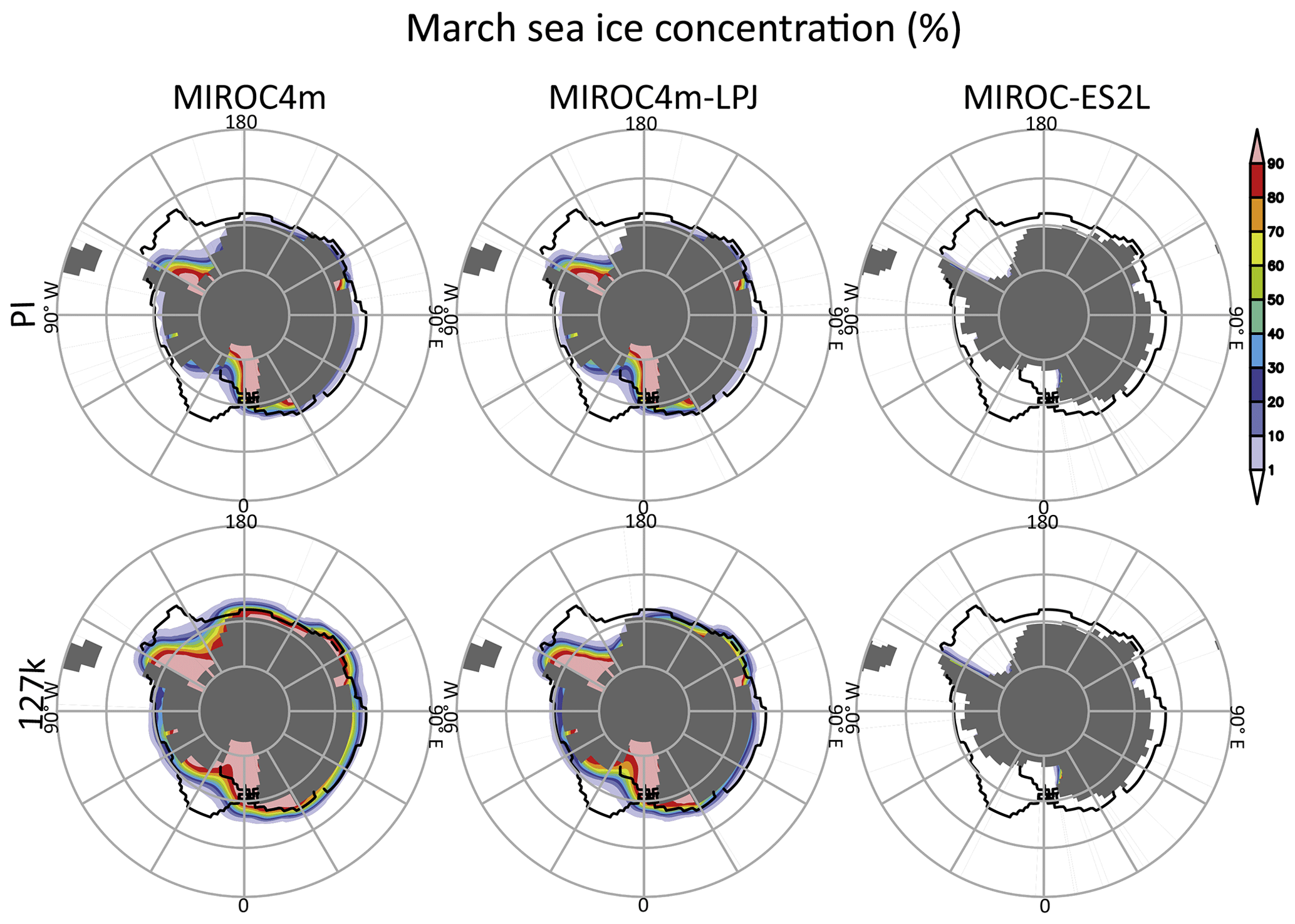
Figure 12 Same as Fig. 10 but for SH March sea ice concentration (%).

Figure 13 Same as Fig. 10 but for SH September sea ice concentration (%).

3.2.3 Vegetation

We compare the vegetation distribution in all three models (Fig. 3) regardless of different treatment (prescribed or predicted). MIROC4m and MIROCES2L adopt a fixed vegetation distribution based on satellite data. The vegetation distribution in MIROC4m is based on the classification of MATSIRO, translated from actual vegetation by Ramankutty and Foley (1999). MIROC-ES2L is also fixed to a satellite-based vegetation distribution that is translated from satellite data (Matthews, 1983, 1984; Hall et al., 2006). These two vegetation maps show similar patterns of forest and grassland, although they differ in the interpretation of classifications such as C₃ and C₄ or the boundary between forest and tundra. Only MIROC4m-LPJ predicts the vegetation distribution in the present study. The 100-year averaged vegetation distribution in the PI shows characteristics common to the other two satellite-based distributions, except for the overestimation of forests (in the boreal forest band and African tropical forest) and underestimation of grassland (in African savanna and central Eurasia). In the 127k simulation, vegetation changes drastically at northern high latitudes. Tundra is broadly replaced by boreal deciduous forest and almost disappears, reflecting the summer warming in the northern high-latitude land, especially in eastern Siberia and North America. Forestation of tundra regions causes amplification of warming in eastern Siberia and North America, especially in the snow melting season. This northward shift of boreal forest eventually leads to an increase in the annually averaged temperature of eastern Siberia and North America by an additional 3 K compared with LIG warming without vegetation change. Grassland appears over a wide area at the boreal–temperate boundary in both Eurasia and North America due to less precipitation supporting forest growth in 127k. This increase in grassland causes cooling at midlatitudes, especially in Eurasia. In the Sahara, a slight northward expansion of grassland is seen, but MIROC4m-LPJ does not reproduce the so-called “green Sahara” (Larrasoaña et al., 2013). Figure 14 shows JJA zonally averaged precipitation over the Sahara (30^∘ W–20^∘ E). In all models, 127k summer precipitation shifts northward compared to PI. MIROC4m-LPJ shows the largest northward shift of precipitation.

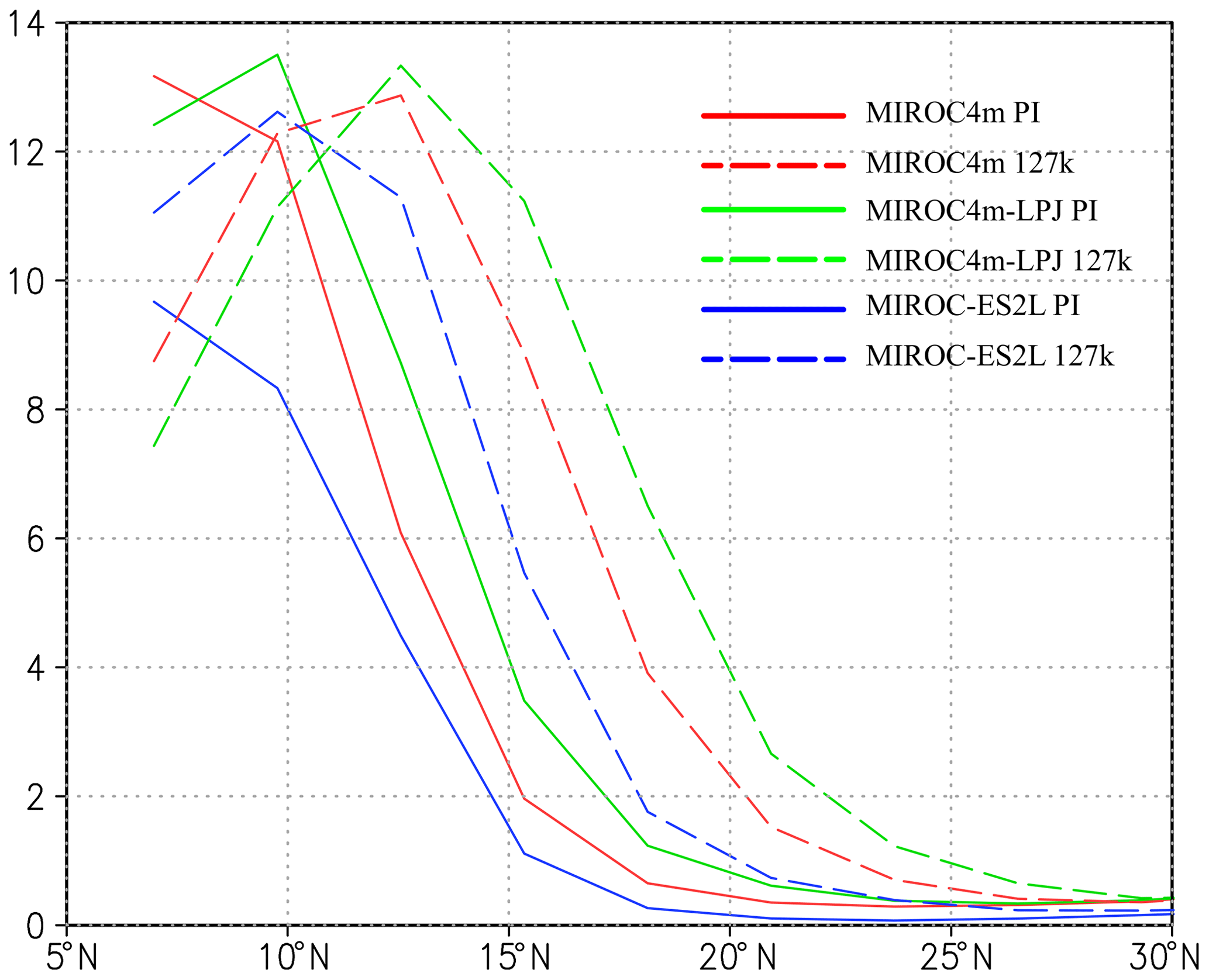
Figure 14 Zonally (30^∘ W–20^∘ E) averaged JJA precipitation (mm d⁻¹) over land at 5–30^∘ N. The calendar for 127k is adjusted using a method based on Bartlein and Shafer (2019).

4 Conclusion and discussion

In the present study, we examined the LIG and PI simulations in accordance with the PMIP4 protocol by using three different versions of the MIROC AOGCM. These three models show a similar response of temperature to the LIG boundary conditions, i.e., warming in boreal summer and cooling in boreal winter (Fig. 4). However, the annually averaged temperature is different among the models. Only MIROC4m-LPJ predicts annual warming at NH high latitudes that is qualitatively consistent with proxy data such as in Turney and Jones (2010), Capron et al. (2017), and Hoffman et al. (2017), while the other two models show a cooling at NH high latitudes. Capron et al. (2014, 2017) noted that the proxies in Turney and Jones (2010) were based on peak warmth values throughout the LIG, and thus the 127k result would not be directly comparable with Turney and Jones (2010). Although it would be more appropriate to compare the modeled LIG result with time slice proxy data at 127 ka from time series reconstructions (Capron et al., 2017; Hoffman et al., 2017), Turney and Jones (2010) provide a large-scale pattern of temperature change. Hence, comparisons between the LIG simulation and Turney and Jones (2010) would still be of much value.

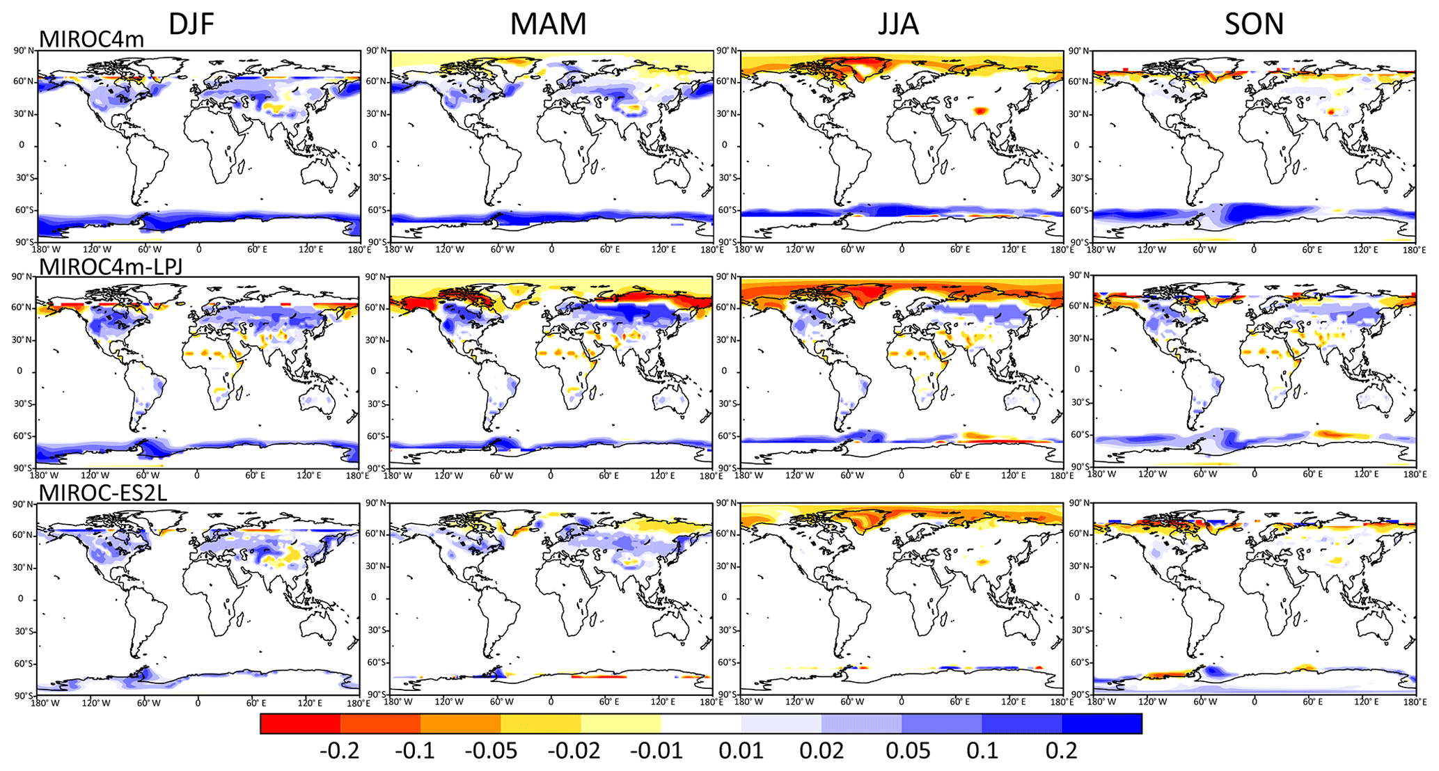
Figure 15 Seasonal surface albedo difference between 127k and PI in three models. The calendar for 127k is adjusted using a method based on Bartlein and Shafer (2019).

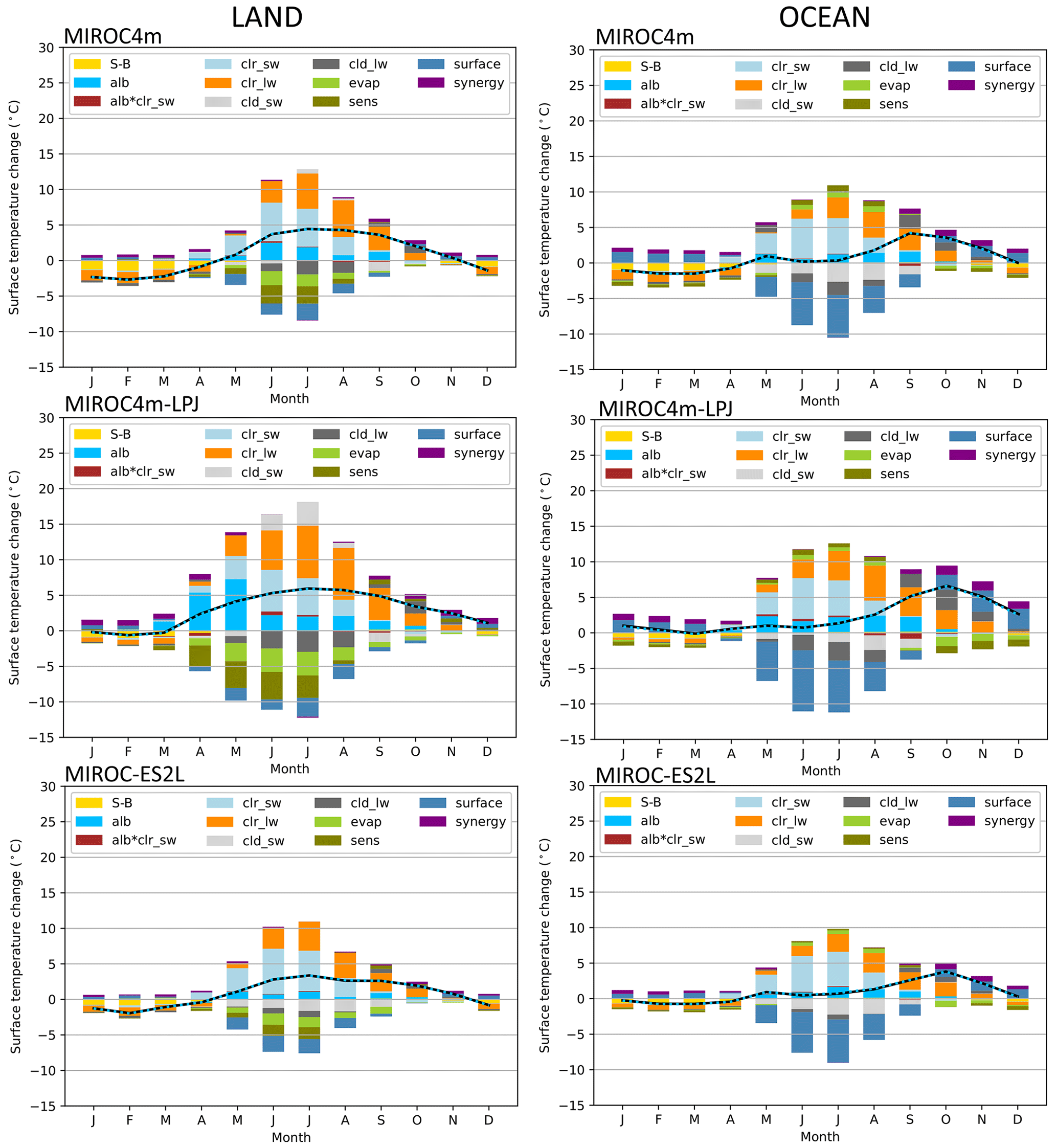
Figure 16 Simulated and diagnosed surface temperature changes (K) in 127k from PI for the land and the ocean (north of 60^∘ N). The solid black polygonal lines denote simulated changes, and dashed blue lines denote the sum of the diagnosed partial changes; the two lines are superimposed. See Table 3 for the interpretation of each component.

The vegetation change seen in MIROC4m-LPJ simulations is a reasonable response to temperature change induced by modifications in orbital parameters. The largest change is the northward shift of boreal forest and expansion of grassland at midlatitudes. By comparing MIROC4m-LPJ and MIROC4m, we suggest that the vegetation feedback mechanism is necessary to explain the temperature change reconstructed by proxies since MIROC4m-LPJ predicts warming closer to reconstructions. By considering the overestimation of boreal forest in PI, vegetation feedback may still be underestimated in MIROC4m-LPJ. The introduction of dynamical vegetation in MIROC4m-LPJ appears to amplify the warming not only over land but also in the ocean at NH high latitudes. On the other hand, MIROC-ES2L, which partially introduces a vegetation effect through LAI prediction, does not show enough warming in the LIG and even shows annual cooling over land at northern high latitudes. In the Arctic Ocean, all three models show warming in SON, in spite of less solar irradiance with 127 ka orbital parameters. This can be considered to be the same as an interseasonal effect of warming in the Arctic Ocean shown by Laîné et al. (2016) and Yoshimori and Suzuki (2019). They analyzed the energy balance and concluded that heat is stored in the Arctic Ocean during summer and emitted in autumn and winter, which causes a larger warming in autumn and winter than in summer. This commonly occurs in CO₂-induced cases (Laîné et al., 2016) and orbitally induced cases (Yoshimori and Suzuki, 2019). In the present study, this mechanism occurs in MIROC4m, without vegetation feedback, and is amplified in MIROC4m-LPJ by vegetation feedback. The largest land surface albedo change occurs in spring (Fig. 15) caused by surface albedo feedback due to the snow-masking effect of trees in MIROC4m-LPJ. The additional energy input to land due to the reduction of albedo is transferred to the Arctic Ocean, where it reduces sea ice and is stored as heat in the ocean. This leads to the largest Arctic warming occurring in autumn through heat release from the ocean in all three models. To confirm this mechanism, we applied the same feedback analysis method as Yoshimori and Suzuki (2019) and obtained the monthly decomposed contribution of energy flux terms to the surface temperature change between 127k and PI in northern high-latitude land and ocean (Fig. 16 and Table 3). The result shows a strong land albedo effect in April and May with MIROC4m-LPJ. The corresponding ocean heat uptake is largest in MIROC4m-LPJ. In autumn and winter, heat is released from the ocean. These results indicate that vegetation feedback, including changes in vegetation distribution, is necessary to predict past warm climate, and such results have implications for future climate simulations. Compared to observations, MIROC-ES2L shows the most realistic PI distribution of sea ice in the Arctic Ocean owing to a new ice physics model. MIROC4m-LPJ predicts the smallest amount of sea ice in PI among the three models in both March and September because temperature in MIROC4m-LPJ is generally higher than that of MIROC4m over land due to the inclusion of dynamical vegetation. This higher temperature reduces sea ice in the Arctic Ocean in the PI and thus inevitably affects the response of sea ice to higher temperatures in the LIG. On the other hand, in the Southern Ocean, MIROC-ES2L underestimates sea ice extension both in March and September, which leads to an underestimation of feedbacks related to sea ice. To investigate the mechanisms in detail, we are planning a further feedback analysis focusing on the surface energy balance.

Table 3 List of the energy flux terms used in Fig. 16. Row 1 represents the strength of the global mean feedback calculated with local warming sensitivity reproduced from Yoshimori and Suzuki (2019). Rows 2–10 represent the strength of local feedback calculated with global mean warming sensitivity.