the Creative Commons Attribution 4.0 License.
the Creative Commons Attribution 4.0 License.
 | 28 Sep 2021
Does a difference in ice sheets between Marine Isotope Stages 3 and 5a affect the duration of stadials? Implications from hosing experiments
Sam Sherriff-Tadano
Ayako Abe-Ouchi
Akira Oka
Takahito Mitsui
Fuyuki Saito
Glacial periods undergo frequent climate shifts between warm interstadials and cold stadials on a millennial timescale. Recent studies show that the duration of these climate modes varies with the background climate; a colder background climate and lower CO2 generally result in a shorter interstadial and a longer stadial through its impact on the Atlantic Meridional Overturning Circulation (AMOC). However, the duration of stadials is shorter during Marine Isotope Stage 3 (MIS3) than during MIS5, despite the colder climate in MIS3, suggesting potential control from other climate factors on the duration of stadials. In this study, we investigate the role of glacial ice sheets. For this purpose, freshwater hosing experiments are conducted with an atmosphere–ocean general circulation model under MIS5a and MIS3 boundary conditions, as well as MIS3 boundary conditions with MIS5a ice sheets. The impact of ice sheet differences on the duration of the stadials is evaluated by comparing recovery times of the AMOC after the freshwater forcing is stopped. These experiments show a slightly shorter recovery time of the AMOC during MIS3 compared with MIS5a, which is consistent with ice core data. We find that larger glacial ice sheets in MIS3 shorten the recovery time. Sensitivity experiments show that stronger surface winds over the North Atlantic shorten the recovery time by increasing the surface salinity and decreasing the sea ice amount in the deepwater formation region, which sets favorable conditions for oceanic convection. In contrast, we also find that surface cooling by larger ice sheets tends to increase the recovery time of the AMOC by increasing the sea ice thickness over the deepwater formation region. Thus, this study suggests that the larger ice sheet during MIS3 compared with MIS5a could have contributed to the shortening of stadials in MIS3, despite the climate being colder than that of MIS5a, because surface wind plays a larger role.
- Article
(3547 KB) - Full-text XML
-
Supplement
(1481 KB) - BibTeX
- EndNote


Reconstructions from ice cores reveal that the climate varied frequently on a millennial timescale over the glacial period (Kawamura et al., 2017). These millennial-scale climate variabilities are known as Dansgaard–Oeschger (DO) cycles and occurred more than 20 times over the last glacial period (DO cycles, Fig. 1; Dansgaard et al., 1993; Huber et al., 2006; Capron et al., 2010; Kindler et al., 2014). The DO cycles are famous for their abrupt and large temperature increases over Greenland from stadial to interstadial, followed by gradual cooling and a drastic return to stadial conditions. These two contrasting climate modes persist for more than several hundred years, and in total, result in periodicity from 1000 years to more than 5000 years (Buizert and Schmittner, 2015; Kawamura et al., 2017). The DO cycles are often attributed to reorganizations of the Atlantic Meridional Overturning Circulation (AMOC) between a vigorous mode and a weak mode (Ganoploski and Rahmstrof, 2001; Piotrowski et al., 2005; Menviel et al., 2014; Henry et al., 2016; Menviel et al., 2020). For example, it is shown that the shift of the AMOC from a vigorous mode to a weak mode causes a reduction of northward oceanic heat transport in the Atlantic, expansion of sea ice and drastic cooling over the North Atlantic and warming over the Southern Ocean (Kageyama et al., 2010, 2013).
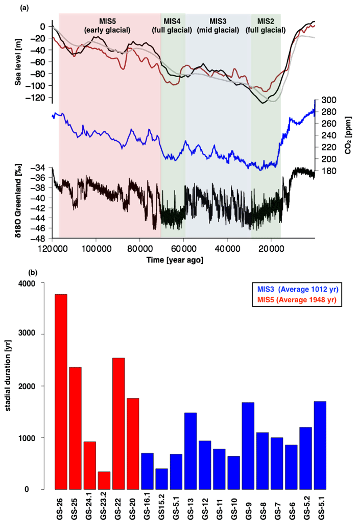
Figure 1(a) Changes in ice volume (sea level, black: Spratt and Lisiecki, 2016; brown: Grant et al., 2012; gray: Abe-Ouchi et al., 2013), CO2 (Bereiter et al., 2015) and Greenland ice core δ18O (a proxy of temperature, Rasmussen et al., 2014) over the last glacial–interglacial cycle. (b) Duration of stadials during MIS5 and MIS3. Color shading in panel (a) separates the period within one glacial cycle. Green: MIS2, MIS4; blue: MIS3; and red: MIS5a–d. During MIS2 and MIS4, the glacial ice sheets were most extensive and the CO2 concentration was low. During MIS3, the glacial ice sheets were relatively small and the CO2 concentration was higher than those of MIS2 and MIS4. During MIS5a–d, the glacial ice sheets were smallest and the CO2 concentration was highest among the glacial periods.
To better understand the dynamics of DO cycles as well as the spread in the duration of DO cycles, previous studies investigate possible relations between the frequency of these cycles and the background climate such as glacial ice sheet amounts and atmospheric CO2. For example, McManus et al. (1999) suggest that DO cycles occur most frequently when the size of the glacial ice sheets is at an intermediate level between interglacial and full glacial. They suggest that intermediate ice sheets can be unstable, and that the frequent release of freshwater can cause drastic weakening of the AMOC. On the other hand, ice core and modeling studies suggest the importance of global cooling in determining the frequency of DO cycles (Buizert and Schmittner, 2015; Kawamura et al., 2017). Kawamura et al. (2017) show that DO cycles occur most frequently when the Antarctic temperature and global cooling are at intermediate levels between interglacial and full glacial periods over the last 720 000 years. It is further demonstrated based on climate modeling experiments that the vigorous AMOC becomes more vulnerable to perturbations such as freshwater hosing when the global or Southern Ocean climate is colder than the modern climate but not as cold as the full glacial climate, resulting in a more unstable vigorous AMOC mode during mid-glacial periods (Buizert and Schmittner, 2015; Kawamura et al., 2017). These results suggest that the spread of the frequency of DO cycles may not purely result from chaotic behavior of the AMOC, but rather may be modulated by changes in the background climate (Buizert and Schmittner, 2015; Kawamura et al., 2017; Mitsui and Crucifix, 2017).
Recent studies of ice cores from both Greenland and Antarctica further explore the relation of the background climate and the frequency of DO cycles by separating the durations of interstadials and stadials. With respect to interstadials, Buizert and Schmittner (2015) show that the duration decreases as Antarctic temperature decreases from interglacial to full glacial conditions (Fig. 1). Lohmann and Ditlevsen (2019) also show, based on ice core data from Greenland, that the duration of interstadials is highly correlated with the surface cooling rate over the northern North Atlantic; the duration decreases as the cooling rate of the Greenland temperature increases. These studies are supported by experiments with climate models showing an increased sensitivity of the vigorous AMOC to freshwater hosing under colder climates (Zhang et al., 2014b; Kawamura et al., 2017) and by climate model studies showing shortening of the duration of interstadials in their intrinsic millennial-scale climate variability with lower CO2 levels (Brown and Galbraith, 2016; Klockmann et al., 2018).
With respect to stadials, the situation is different. Buizert and Schmittner (2015) find a weak relation between the durations of stadials and Antarctic temperature; the durations of the stadials are extremely long during the full glacial interval (Marine Isotope Stage (MIS) 2, 4, Fig. 1a), short in the early glacial interval (MIS5) and even shorter in the mid-glacial period (MIS3, Fig. 1b), which contributes to the short periodicity of DO cycles during mid-glacial periods. In addition, Lohmann (2019) analyze the dust record in Greenland ice cores and find that the durations of stadials correlate with the decreasing trend of dust during the first 100 years of the stadials. Although the factors controlling the trend of dust remain unclear, these results suggest that another type of climate forcing over the North Atlantic plays a role in modulating the durations of stadials in combination with surface cooling. In addition, these results suggest that the processes modulating durations of interstadials and stadials may differ. Nevertheless, it still remains unclear why the durations of stadials are generally shorter in MIS3 compared with MIS5, despite colder conditions in MIS3.
From a climate modeling point of view, previous studies investigate dependence of the recovery time of the AMOC and the duration of stadials to the background climate, based on freshwater hosing experiments. While the timing of freshwater input and DO cycles is still debated, and while freshwater hosing may not be the cause of the AMOC weakening (Barker et al., 2015), these studies provide useful information to study DO cycles. For example, Weber and Drijhout (2007) and Bitz et al. (2007) show that the recovery time of the AMOC is longer under glacial conditions (Last Glacial Maximum, LGM) compared with pre-industrial (PI) conditions. These studies suggest that a larger expansion of sea ice over the North Atlantic in the LGM causes an increase in the recovery time of the AMOC. Extensive sea ice covers the original deepwater formation regions and suppresses atmosphere–ocean heat exchange in the deepwater formation region (Oka et al., 2012, 2021; Sherriff-Tadano and Abe-Ouchi, 2020), which makes it difficult for the AMOC to recover after freshwater hosing is ceased (Bitz et al., 2007; Weber and Drijhout, 2007). In contrast, Gong et al. (2013) compare the recovery time of the AMOC under PI, mid-glacial and LGM conditions in a comprehensive climate model and find that the recovery time is shortest in the mid-glacial case and longest in the PI case. They suggest that greater subsurface ocean warming over the deepwater formation region, which affects ocean stratification (Mignot et al., 2007), is important in causing a shorter recovery time of the AMOC in the mid-glacial period. Furthermore, Goes et al. (2019) recently show that the recovery time of the AMOC becomes shorter when they force their Earth system model of intermediate complexity (EMIC) with LGM winds compared with modern winds. These results support the inference that changes in the background climate (e.g., ice sheet configurations and insolation) can modify the duration of stadials, although the processes and results may depend on the models used. However, in most studies, because the boundary conditions such as ice sheet configurations, CO2 concentration and insolation are all modified at the same time, the impacts of individual boundary conditions on the durations of stadials and the recovery time of the AMOC remain elusive. A better understanding of the individual roles of boundary conditions and their mechanism in modifying the recovery time is necessary to understand the changes in the durations of stadials across glacial periods, as well as to interpret model discrepancies.
Previously, it was shown that large Northern Hemisphere glacial ice sheets increase sea surface salinity over the North Atlantic Deep Water (NADW) formation region by increasing surface winds and decreasing precipitation (Eisenman et al., 2009; Smith and Gregory, 2012; Brady et al., 2013; Zhang et al., 2014a; Gong et al., 2015; Klockmann et al., 2016; Galbraith and de Lavergne, 2019; Guo et al., 2019). In addition, it was shown that stronger surface cooling by ice sheets increases the amount of sea ice in the NADW formation region and the Southern Ocean, the latter of which is induced by colder NADW outcropping in the Southern Ocean (Sherriff-Tadano et al., 2021a). These results imply that differences in glacial ice sheets may play a role in modifying the durations of stadials during glacial periods. Recently, Sherriff-Tadano et al. (2021a) performed simulations of MIS3 and MIS5a and explored the impact of ice sheet differences on the AMOC and climate. In their simulations, differences in ice sheets exert small impacts on the vigorous mode of the AMOC, because of a compensational balance between the increase in sea surface salinity in the northern North Atlantic (strengthening effect) and the increase in sea ice in the North Atlantic and Southern Ocean (weakening effect). However, the impact of mid-glacial ice sheets on the duration of stadials and the recovery time of the AMOC remains elusive. Because the important processes affecting the stability of the AMOC may differ between vigorous and weak AMOC modes (Buizert and Schmittner, 2015; Lohmann, 2019), a different response of the AMOC to ice sheet forcing under a weak AMOC state may be found.
In this study, we explore the impacts of differences in the ice sheets between the MIS3 and MIS5a on the recovery time of the AMOC and the durations of stadials. For this purpose, we perform freshwater hosing experiments under three background climates that have been simulated previously, MIS3, MIS5a and MIS3 with the ice sheet forcing of MIS5a (Sherriff-Tadano et al., 2021a). By comparing the recovery time of the AMOC after the cessation of freshwater hosing in each experiment, we assess the impact of the ice sheets on the recovery time of the AMOC. Furthermore, to explore the mechanism by which the ice sheets modify the recovery time of the AMOC, we perform partially coupled experiments. In these experiments, the atmospheric forcing, which is passed to the oceanic component of the model, is replaced with a different forcing. By this method, individual effects of changes in surface wind, atmospheric freshwater flux, or surface cooling on the AMOC can be estimated (Mikolajewicz et al., 2000; Schmittner et al., 2002; Gregory et al., 2005; Sherriff-Tadano et al., 2021a).
We should note that, in the hosing experiments, we focus on how the climate system recovers from the cessation of external forcing. In contrast, recent studies with atmosphere–ocean coupled general circulation models (AOGCMs) show intrinsic oscillations of AMOC, which resemble DO cycles, without any external forcing. For example, Vettoretti and Peltier (2016) and Sherriff-Tadano and Abe-Ouchi (2020) show in their intrinsic oscillations of AMOC that the recovery of the AMOC from weak mode to strong mode is determined by the balance among sea ice, surface salinity and subsurface ocean warming over the deepwater formation region in the North Atlantic. From the viewpoint of mechanisms, the recovery process of the AMOC in the present hosing experiments is similar to that in the intrinsic oscillations of AMOC. Therefore, our findings may not be confined to the hosing experiments or DO cycles induced by external forcing but may also be applied to those obtained via intrinsic oscillations of the AMOC.
This paper is organized as follows. Section 2 describes the model and the experimental design. In Sect. 3, the impacts of the ice sheet configurations on the recovery time of the AMOC and its mechanism are assessed. Section 4 discusses the results, and Sect. 5 presents the conclusion.
2.1 Model
Numerical experiments are performed with the Model for Interdisciplinary Research on Climate 4m (MIROC4m; Hasumi and Emori, 2004), an AOGCM. This model consists of an atmospheric general circulation model (AGCM) and an oceanic general circulation model (OGCM). The AGCM and OGCM include a land surface model and a sea ice model, respectively. The AGCM solves the primitive equations on a sphere using a spectral method. The horizontal resolution of the atmospheric model is ∼ 2.8∘, and there are 20 layers in the vertical direction. The OGCM solves the primitive equations on a sphere, with the Boussinesq and hydrostatic approximations adopted. The horizontal resolution is ∼ 1.4∘ in longitude and 0.56–1.4∘ in latitude (latitudinal resolution is finer near the Equator). There are 43 layers in the vertical direction. Note that the coefficient of horizontal diffusion of the isopycnal layer thickness in the OGCM is increased to 700 m2 s−1 compared with the original model version (300 m2 s−1) that was submitted to Paleoclimate Model Intercomparison Project 2. These two model versions are referred to as Model B and Model A, respectively, by Sherriff-Tadano and Abe-Ouchi (2020). Here, we use Model B. The model version used in this study has been used extensively for modern climate, paleoclimate (Obase and Abe-Ouchi, 2019; O'ishi et al., 2021; Chan and Abe-Ouchi, 2020) and future climate studies (Yamamoto et al., 2015). It also reproduces the AMOC of the present, LGM (Sherriff-Tadano and Abe-Ouchi, 2020), MIS3 and MIS5a (Sherriff-Tadano et al., 2021a) reasonably well. See Hasumi and Emori (2004) and Chan et al. (2011) for detailed information on the parameterizations used in the model.
2.2 Model simulations
This study is based on three climate simulations that have been performed previously (Sherriff-Tadano et al., 2021a, Table 1). The first climate simulation is that of MIS5a, which is forced with a CO2 concentration of 240 ppm, insolation of 80 ka and the ice sheet boundary configuration of 80 ka taken from Ice sheet model for Integrated Earth system Studies (IcIES, Abe-Ouchi et al., 2007, 2013, Fig. 2a). The second and third climate simulations are those of MIS3, both of which are forced with CO2 of 200 ppm and insolation of 35 ka but forced with ice sheets of either 36 ka (MIS3, Fig. 2b) or 80 ka (MIS3–5aice, Table 1). The volumes of the ice sheet are 40 m sea level equivalent for 80 ka and 96 m sea level equivalent for 36 ka (Abe-Ouchi et al., 2013). The volume of the MIS3 ice sheets exceeds the range of reconstructions (40 to 90 m sea level equivalent; Grant et al., 2012; Spratt and Lisiecki, 2016; Pico et al., 2017; Gowan et al., 2021); hence, this may cause an overestimation of the ice sheet effect. Nevertheless, the ice sheet forcing used in this study at least captures the characteristics suggested by reconstructions, which show larger ice sheets at MIS3 compared to MIS5a (Pico et al., 2017; Gowan et al., 2021). The Antarctic ice sheet is fixed to the modern configuration, and the Bering Strait is open in all experiments. For methane and other greenhouse gases, the concentration of the LGM is used (Dallenbach et al., 2000). These three simulations are initiated from a previous LGM experiment by Kawamura et al. (2017) and are integrated for 2000 years (MIS5a) or 3000 years (MIS3 and MIS3–5aice). The decreasing trends of deep ocean temperature of the last 100 years are 0.002 ∘C in MIS5a, 0.011 ∘C in MIS3 and 0.007 ∘C in MIS3–5aice, respectively (Sherriff-Tadano et al., 2021a).
Table 1Forcing and boundary conditions of the climate simulations.
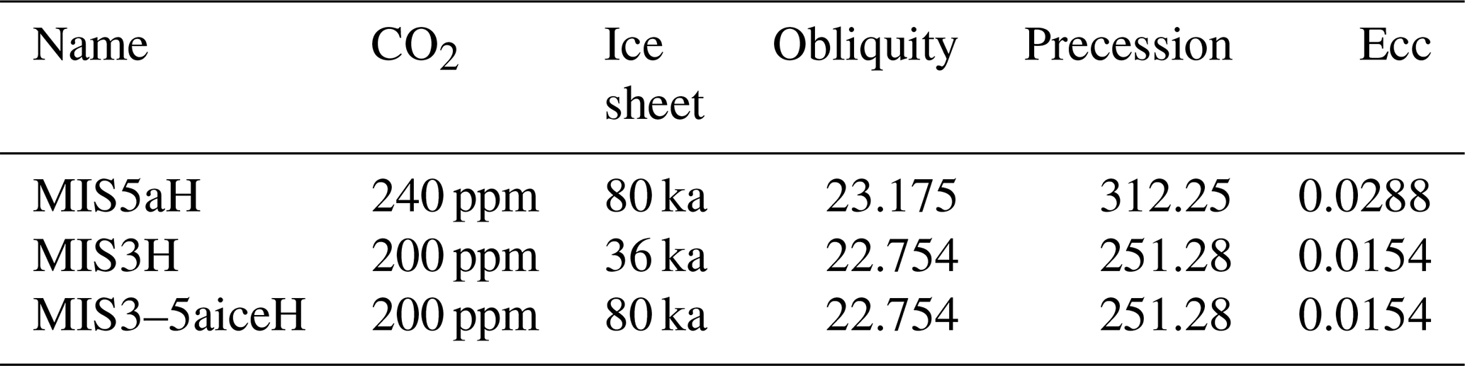
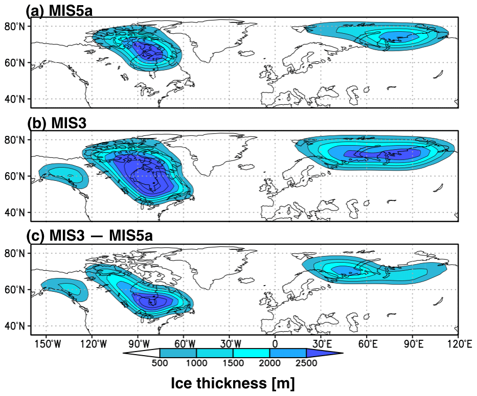
Figure 2Ice sheet thickness of (a) MIS5a (80 ka), (b) MIS3 (36 ka) and (c) MIS3 minus MIS5a. Results from an ice sheet model are presented (Abe-Ouchi et al., 2013). These ice sheet configurations were used for climate model simulations.
To cause drastic weakening of the AMOC and shift the climate into stadial, a freshwater flux of 0.1 Sv is applied uniformly over the northern North Atlantic (50–70∘ N) for 500 years (Fig. 3). Subsequently, the freshwater flux is stopped and the experiments are further integrated for 1000 years to assess the dependence of the recovery time on the background climate. These experiments are named MIS3H, MIS5aH and MIS3–5aiceH, respectively (Table 1). The impact of the mid-glacial ice sheet on the duration of stadials is assessed by comparing the recovery time of the AMOC between MIS3H and MIS3–5aiceH (Table 1). The effect of the differences in CO2 and insolation can be assessed by comparing the recovery time of the AMOC between MIS3–5aiceH and MIS5aH (Table 1).
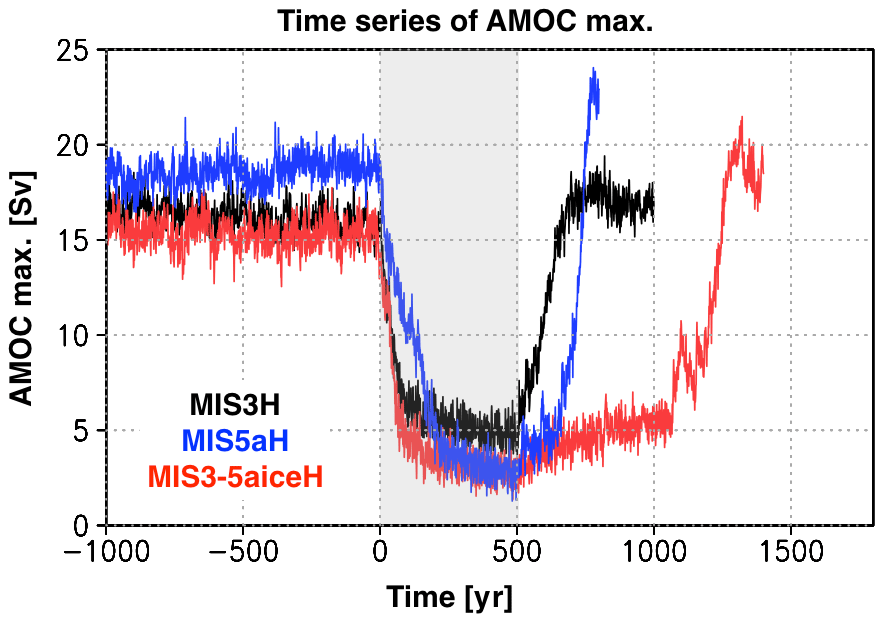
Figure 3Time series of the strength of the AMOC under freshwater hosing. Freshwater of 0.1 Sv was released to 50–70∘ N in the North Atlantic for 500 years from year 1 (gray-shaded period). Black: MIS3H, blue: MIS5aH, and red: MIS3–5aiceH.
2.3 Partially coupled experiments
To clarify the mechanisms by which glacial ice sheets modify the recovery time of the AMOC, partially coupled experiments are conducted (Table 2). In these experiments, the atmospheric forcing – wind stress and atmospheric freshwater flux (precipitation, evaporation and river runoff) – is replaced with monthly climatologies. The heat flux is unchanged in these experiments, as it is strongly coupled with the sea surface temperature and fixing the surface heat conditions has an unrealistic impact on the AMOC (Schmittner et al., 2002; Gregory et al., 2005; Marozke, 2012). Atmospheric forcing is replaced with monthly climatologies of the last 100 years of the hosing period in each experiment. Thus, this forcing does not include atmospheric noise, which itself can induce a mode shift of the AMOC (Kleppin et al., 2015). Nevertheless, a similar conclusion is obtained when raw daily fields obtained from the last 100 years of the hosing period are used instead of monthly climatologies (Fig. S1 in the Supplement). Understanding the role of atmospheric noise is beyond the scope of this study but should be explored in other studies.
Table 2List of partially coupled experiments. In each of these experiments, atmospheric forcing was replaced by the monthly climatologies of the specified experiment.
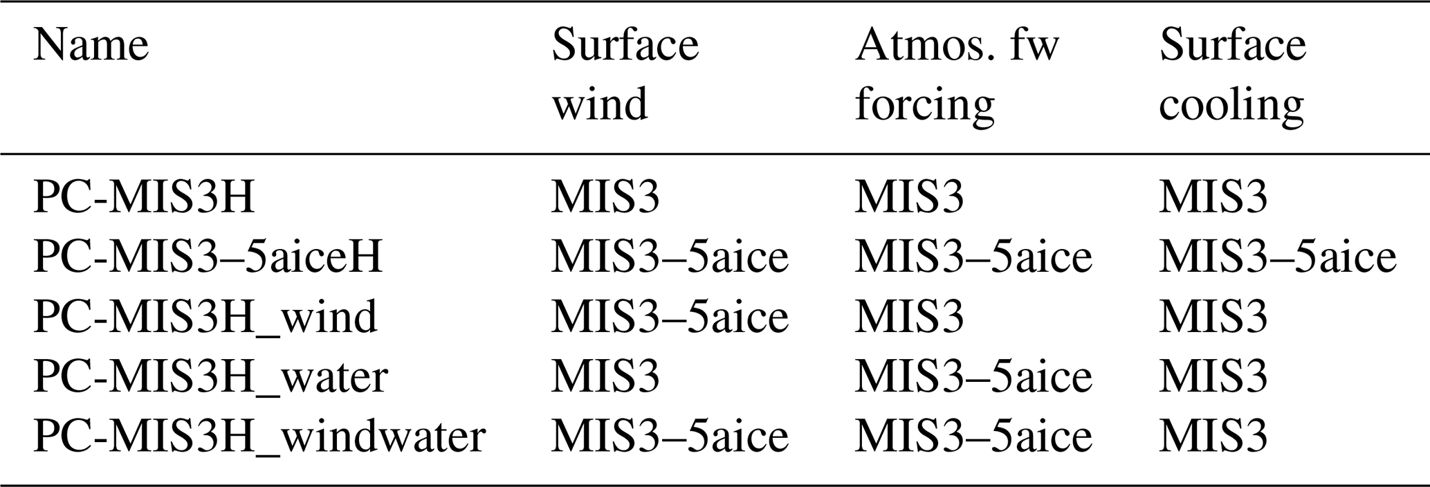
Five partially coupled experiments are conducted under MIS3H and MIS3–5aiceH (Table 2). All of the experiments are initiated from the first year of the cessation of freshwater hosing, which correspond to the period when the climate and AMOC have settled to the stadial state (see Figs. 11 and 12). The first two experiments serve as a validation of the method; the atmospheric forcing is replaced with the monthly climatologies in MIS3H and MIS3–5aiceH. These experiments are named PC-MIS3H and PC-MIS3–5aiceH, respectively. We regard the method as valid when these experiments reproduce the general difference of MIS3H and MIS3–5aiceH. In the other three experiments, the atmospheric forcing is replaced with different forcing (Table 2). In PC-MIS3H_wind, the surface wind stress of MIS3–5aiceH is applied to MIS3H. In PC-MIS3H_water, the atmospheric freshwater flux of MIS3–5aiceH is applied to MIS3H. In PC-MIS3H_windwater, the atmospheric freshwater flux and surface wind stress of MIS3–5aiceH are applied to MIS3H. From these experiments, the impact of differences in the wind is estimated as the difference between PC-MIS3H_wind and PC-MIS3H, the impact of differences in the atmospheric freshwater flux is estimated as the difference between PC-MIS3H_water and PC-MIS3H, and the impact of differences in the surface cooling is estimated as the difference between PC-MIS3H_windwater and PC-MIS3–5aiceH (Table 2). Note that the effect of surface cooling (heat flux) is estimated as a residual, following previous studies (Gregory et al., 2005). The surface cooling effect includes the effects of changes in freshwater flux of sea ice.
In conducting partially coupled experiments, the location of atmospheric freshwater flux needs to be adjusted following differences in land–sea mask between MIS3 and MIS5a ice sheets (Fig. S2). The largest changes appear over the Barents Sea, where new ice sheets expand. In contrast, changes in land–sea mask near the Labrador Sea and Norwegian Sea, where the main oceanic convections take place (Fig. 5), are small (Fig. S2). We adjust the location of river runoff and atmospheric freshwater flux in the partially coupled experiment by shifting it to closest ocean grid points.
Simulated climates of unperturbed MIS5a, MIS3 and MIS3–5aice are displayed in Figs. 3–5. The simulated global air temperatures are 10.6 ∘C in MIS5a, 7.9 ∘C in MIS3 and 8.9 ∘C in MIS3–5aice (Sherriff-Tadano et al., 2021a). The maximum strength of the AMOC is 18.4 Sv in MIS5a, 15.6 Sv in MIS3 and 15.1 Sv in MIS3–5aice (Fig. 4). The slightly weaker AMOC in MIS3 than in MIS5a is consistent with a reconstruction based on 231Pa 230Th (Bohm et al., 2015). Associated with the vigorous AMOC, deepwater forms in the Greenland Sea and the Irminger Sea, and most parts of the northern North Atlantic remain ice-free in all experiments (Fig. 5). These characteristics are consistent with proxy data suggesting ice-free conditions in the Norwegian Sea during interstadials (Dokken et al., 2013; Sadatzki et al., 2019).
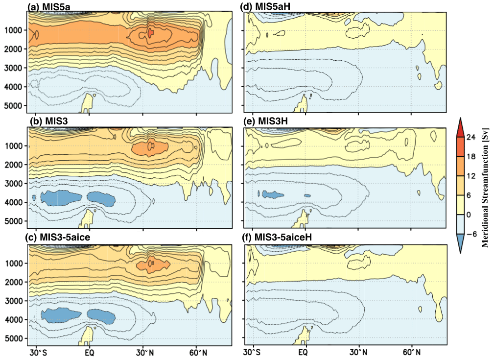
Figure 4Meridional streamfunction (Sv = 106 m3 s−1) in the Atlantic. (a) MIS5a, (b) MIS3, (c) MIS3–5aice, (d) MIS5aH, (e) MIS3H, and (f) MIS3–5aiceH. The last 100 years are used for analysis.
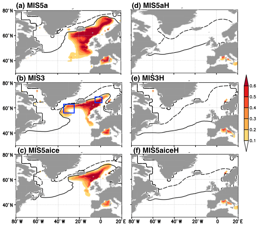
Figure 5Sea ice edge (contour, 50 % concentration) for February (solid) and August (dashed) and deepwater formation region shown in annually averaged frequency of the convective adjustment at 300 m depth (color). (a) MIS5a, (b) MIS3, (c) MIS3–5aice, (d) MIS5aH, (e) MIS3H, and (f) MIS3–5aiceH. In panels (a)–(c), deepwater formation regions before the hosing are displayed, while in panels (d)–(f), deepwater formation regions of the last 100 years of the hosing period are shown. In panel (b), areas used for time series analysis in Figs. 8 and 12 are shown in blue rectangles.
3.1 Responses to freshwater hosing
To shift the climate and AMOC into stadial states, freshwater hosing experiments are performed under these background climate conditions. These experiments all show drastic weakening of the AMOC in response to hosing (Figs. 3 and 4). The strength of the AMOC decreases to 3 Sv in MIS5aH and MIS3–5aiceH, and decreases to 5 Sv in MIS3H. In addition, the Antarctic bottom water further penetrates into the North Atlantic compared with unperturbed conditions (Fig. 4). Associated with the weakening of the AMOC, sea ice expands farther south and reaches 50∘ N (Fig. 5). As a result, the deepwater formation region is covered by sea ice and the sea surface temperature over the northern North Atlantic is drastically reduced (Fig. 6). In addition, the surface salinity decreases drastically at high latitudes (Fig. 6) because of freshwater hosing, cessation of convective mixing and a reduction in northward salt transport by the AMOC. In contrast, the subsurface ocean temperature increases at high latitudes because of the suppression of convective mixing. These characteristics are consistent with proxies (Rasmussen and Thomsen, 2004; Dokken et al., 2013). In the tropics, the subsurface ocean temperature and salinity increase because of the weakening of the northward transport of heat and salt by the AMOC (Gong et al., 2013).
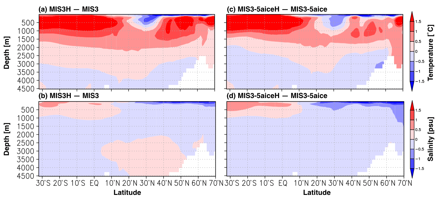
Figure 6Oceanic responses to freshwater hosing in MIS3 (a, b) and MIS3–5aice (c, d). Figures on the top show annual mean ocean temperature anomalies (∘C, color), and figures on the bottom show salinity anomaly (psu, color). Differences between the last 100 years of hosing and the last 100 years before hosing are shown.

Figure 7Atmospheric responses to freshwater hosing in MIS3–5aiceH. (a) Annual mean surface air temperature (∘C, color) and (b) precipitation anomaly (cm d−1, color). Differences between the last 100 years of hosing and last 100 years before hosing are shown.
The weakening of the AMOC and the expansion of sea ice induce drastic cooling over Greenland (Fig. 7a). In particular, the February temperature decreases by 12 ∘C in MIS3H, 10 ∘C in MIS3–5aiceH and 12 ∘C in MIS5aH, which are within the range of ice core data (Kindler et al., 2014). Over the Antarctic, the temperature increases by 1–2 ∘C because of the bipolar seesaw (Kawamura et al., 2017). In terms of precipitation (Fig. 7b), the model reproduces a southward shift of the tropical rain belt (Wang et al., 2004) and weakening of the Indian monsoon (Deplazes et al., 2014). Therefore, the model reproduces the overall characteristics of the climate shift into stadial reasonably well.
3.2 Recovery
The AMOC recovers from the weak state to the vigorous state in all experiments after the cessation of freshwater hosing (Fig. 3), although the recovery time differs among the experiments. In MIS5aH, the AMOC starts to recover abruptly 200 years after the cessation of hosing. In MIS3H, the AMOC first increases by 4.5 Sv over the first 80 years and then intensifies abruptly to the vigorous mode by 7.1 Sv in 70 years (the recovery speed nearly doubled compared with the first 80 years). The recovery time is 100 years shorter in MIS3H compared with MIS5aH, which is consistent with the ice core data showing slightly shorter durations of stadials during MIS3 compared with MIS5a–d (Buizert and Schmittner, 2015). In contrast, the recovery time is much longer in MIS3–5aiceH; it takes approximately 600 years to start the drastic recovery. Before that, the AMOC recovers gradually by 3 Sv over the first 560 years. Around model year 1065, the AMOC is abruptly enhanced to 10 Sv. The strength of the AMOC then decreases to 7 Sv, although 100 years after the first abrupt strengthening, the AMOC starts to recover abruptly to the interstadial state. These results reveal three important points. First, the larger mid-glacial ice sheets in MIS3 compared with those of MIS5a shorten the recovery time of the AMOC (comparisons of MIS3H and MIS3–5aiceH). Second, the lowering of the CO2 and the changes in insolation from MIS5aH to MIS3–5aiecH contribute to the increase in the recovery time of the AMOC in our experiments. This is consistent with other studies showing an increase in the durations of stadials under lower CO2 concentrations (Brown and Galbraith, 2016; Klockmann et al., 2018). Third, the recovery time of the AMOC cannot be predicted based on the original strength of the AMOC because the recovery time is shorter in MIS3H compared with MIS5aH, even though the original AMOC is weaker. In MIS3H, the effect of the glacial ice sheet is strong and thus causes shortening of the recovery time compared with MIS5aH, despite having lower CO2 concentration. Below, we further compare the recovery process in MIS3–5aiceH and MIS3H to understand how glacial ice sheets modify the recovery time, which remains unclear in previous studies.
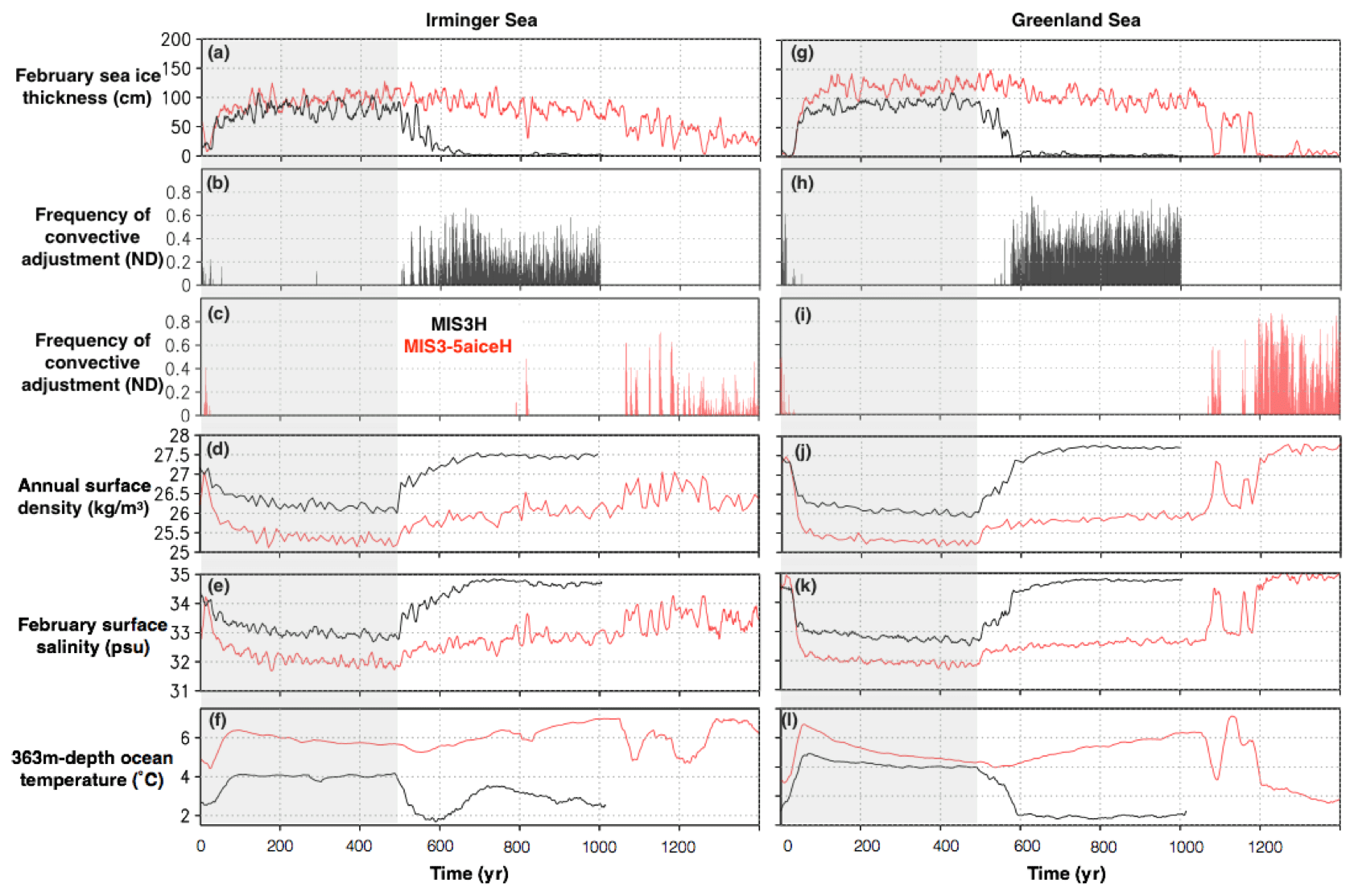
Figure 8Temporal evolution of oceanic variables in the Irminger Sea (55–63∘ N, 35–25∘ W; left) and Greenland Sea (65–70∘ N, 1∘ W–5∘ E; right) for MIS3H (black) and MIS3–5aiceH (red). (a, g) February sea ice thickness (cm). (b, h) Annual average frequency of convective adjustment of MIS3H. (c, i) Same as panels (b) and (h) but for MIS3–5aiceH. (d, j) Annual mean surface density (kg m−3). (e, k) February surface salinity (psu) and (f, l) annual mean subsurface ocean temperature (∘C). Except for panels (b), (c), (h) and (i), 11-year running means are shown. Freshwater flux of 0.1 Sv is applied during years 0 to 500 (gray-shaded period).
To understand the recovery process of MIS3–5aiceH, time series of sea ice, deepwater formation, surface salinity, surface density and subsurface ocean temperature are analyzed (Renold et al., 2010; Vettoretti and Peltier, 2016; Brown and Galbraith, 2016). Figure 8 shows time series of these variables in the Irminger Sea (55–63∘ N, 35–25∘ W) and Greenland Sea (65–70∘ N, 1∘ W–5∘ E), where deepwater forms at the onset of the abrupt recovery of the AMOC. In MIS3–5aiceH, after the cessation of hosing, surface salinity and density first increase in the Irminger Sea and Greenland Sea (red line in Fig. 8d, e, j, k). In association, the AMOC strengthens slightly by 3 Sv over the first 560 years and increases the northward transport of salt and heat. This induces a slight increase in the subsurface temperature and surface salinity and a decrease in sea ice (Fig. 8). During this period, no deepwater forms in Irminger Sea and Greenland Sea, except for one case in the Irminger Sea approximately 300 years after the cessation of hosing (Fig. 8c, year 800 in the figure). Nevertheless, the AMOC does not start to recover at this point (Fig. 3) because the surface salinity and subsurface ocean temperature are not sufficiently high to maintain convection. Then 400 years after the cessation of hosing, the surface salinity and sea ice thickness reach an apparently steady state (Fig. 8a, e), whereas the subsurface temperature continuously increases (Fig. 8f, year 900 in the figure). When the subsurface ocean warms sufficiently, vigorous convective mixing initiates again in the Irminger Sea (Figs. 8c and 9, regions circled by black contours). As a result, a positive salinity anomaly spreads over the subpolar gyre regions (Fig. 9), which causes a second deepwater formation in the northwestern North Atlantic in the Greenland Sea, where the surface salinity is sufficiently high and subsurface ocean sufficiently warm (Figs. 8f and 9). These deepwater formations do not occur continuously and they cease once, possibly associated with decadal variability in deepwater formation (Oka et al., 2006), and are similar to the observation of early warning signals for DO events (i.e., signs of a tipping point) in a high-resolution ice core record (Boers, 2018). However, the deepwater formation in the Greenland Sea induces southward flow through the Denmark Strait in the deep ocean and enhances the AMOC via downward flow along the slope (Renold et al., 2010). As a result, a compensational northward surface flow transports salt into the deepwater formation and causes a second occurrence of convection in the Greenland Sea (Fig. 9, years 1075 to 1079). Subsequently, the AMOC recovers abruptly to its original strength with an overshoot (Fig. 3). These recovery processes show that the balance of sea ice thickness, sea surface salinity and subsurface ocean temperature determine the recovery time of the AMOC in this experiment. The recovery process observed here is also similar to the recovery process of AMOC in intrinsic AMOC oscillations observed in Vettoretti and Peltier (2016) and Sherriff-Tadano and Abe-Ouchi (2020).
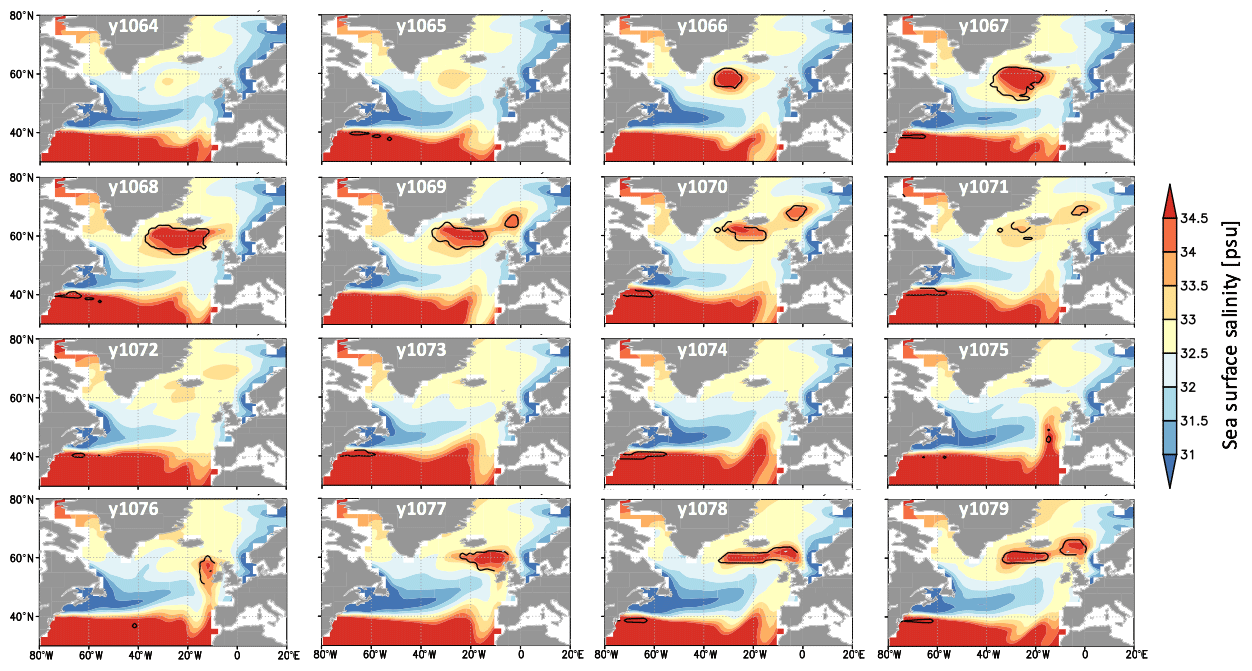
Figure 9Spatial maps of the temporal evolution of surface salinity (color, psu) and the frequency of convective adjustment at 300 m depth (black contours, non-dimensional) in MIS3–5aiceH. Annual means are shown. The value of the contour is 0.1.
In contrast, the recovery process differs in MIS3H (black line in Fig. 8). At first, during the hosing period, sea surface salinity is higher and sea ice thickness is thinner compared with MIS3–5aiceH (Fig. 8a, d, e), which are favorable conditions to induce deepwater formation. Note that at this point, no deepwater forms in the northern North Atlantic (Figs. 5d and 8b, h). After the cessation of freshwater hosing, however, the initial increase of surface salinity triggers deepwater formation in the Irminger Sea (Fig. 8b, e). Because the surface salinity is already sufficiently high in the last 100 years of the hosing period (Fig. 8e), deepwater can form continuously over Irminger Sea (Fig. 8b). As a result, vertical mixing occurs continuously and further increases surface salinity and decreases sea ice thickness over the Irminger Sea and Greenland Sea. The increase in sea surface salinity and density then induces a gradual strengthening of the AMOC by 4.5 Sv in 80 years (Fig. 3). This gradual increase in the AMOC further helps to increase the surface salinity and decrease sea ice thickness over the Greenland Sea (Fig. 8g, j, k). As a result, 80 years after the cessation of hosing, deepwater formation initiates in the Greenland Sea (Fig. 8h), and the AMOC abruptly recovers by 7.1 Sv in 70 years (Fig. 3). Thus, in MIS3H, changes in the surface salinity and sea ice thickness play a larger role in controlling the recovery time of the AMOC, whereas the changes in subsurface ocean temperature play a minor role in the recovery (Fig. 8f, l).
The above analysis suggests that the differences in surface salinity and sea ice between MIS3H and MIS3–5aiceH under the hosing phase cause the difference in the recovery time; in MIS3H, surface salinity is higher and sea ice thickness is thinner compared with MIS3–5aiceH, which favor a shorter recovery time. The differences in sea ice and surface salinity may be attributed to a difference in the surface wind (Sherriff-Tadano et al., 2018). Figure 10a and d show how the surface wind differs in the two experiments. Anomaly fields in Fig. 10d reveal the enhancement of cyclonic wind over the northern North Atlantic and southward displacement of the westerly winds in MIS3H compared with MIS3–5aiceH, which are induced by the topography of the Laurentide ice sheet (Pausata et al., 2011; Sherriff-Tadano et al., 2021a). The southward-shifted westerly wind and strong northerly wind over the western North Atlantic act to reduce the eastward transport of sea ice to the deepwater formation region in MIS3H (Fig. 10c, f). Therefore, even though the atmosphere is colder (Fig. S5), less sea ice exists over the Irminger Sea. In terms of surface salinity, the stronger cyclonic surface winds enhance the Ekman upwelling and gyre circulation that transport saline water to the deepwater formation region and support convection through increasing the surface salinity (Fig. 10b, e; Montoya and Levermann, 2008; Muglia and Schmittner, 2015; Sherriff-Tadano et al., 2018). In fact, a positive wind stress curl is larger in the subpolar region and the Irminger Sea in MIS3H compared with MIS3–5aiceH (Fig. 10d). Therefore, differences in winds over the northern North Atlantic seem to contribute to the difference in the recovery time between the two experiments by modulating the surface salinity and sea ice in the stadial period.
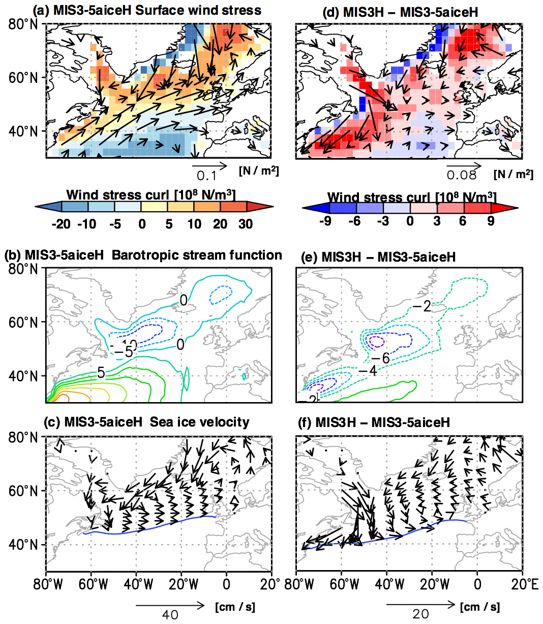
Figure 10Comparison of surface wind and wind-driven oceanic components between MIS3H and MIS3–5aiceH. Annual mean climatology values of (a, d) surface wind stress, (b, e) barotropic streamfunction (m2 s−1) and (c, f) sea ice velocity (cm s−1) are shown. In panels (a), (b) and (c), results from MIS3–5aiceH are shown. In panels (d), (e) and (f), the differences between MIS3H and MIS3–5aiceH are shown. Blue contour lines in panels (c) and (f) show sea ice edges (15 % concentration) of MIS3–5aiceH and MIS3H, respectively. The average over the last 100 years of hosing (years 401–500) is shown.
3.3 Partially coupled experiments
To clarify the impact of differences in surface wind between MIS3H and MIS3–5aiceH on the recovery time of the AMOC, partially coupled experiments are conducted from the first year after the cessation of freshwater hosing (Fig. 11). First, the reproducibility of the original experiments by the partially coupled experiments is assessed. In PC-MIS3H and PC-MIS3–5aiceH, the recovery time is shorter compared with the corresponding original experiments. In particular, the recovery time is 200 to 300 years shorter in PC-MIS3–5aiceH compared with MIS3–5aiceH. This is related to the removal of sub-monthly variations in wind stress (Sherriff-Tadano et al., 2021a, Supplement); removal of these variations causes thinning of sea ice in the center of the subpolar region by reducing sea ice transport in this region (Fig. 12b, c) and creates favorable conditions for deepwater to form. Nevertheless, even though PC-MIS3–5aiceH underestimates the recovery time, PC-MIS3H and PC-MIS3–5aiceH at least reproduce the main difference of the recovery time between MIS3H and MIS3–5aiceH.
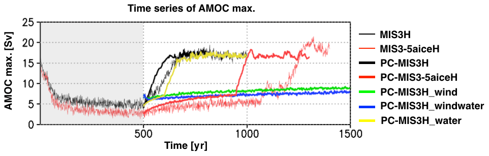
Figure 11Results from partially coupled experiments. Time series of the strength of the AMOC is shown. Results from the original AOGCM experiments are shown by thin lines, whereas the results from partially coupled experiments are shown in thick lines. Thin black: MIS3H, thin red: MIS3–5aiceH, thick black: PC-MIS3H, thick red: PC-MIS3–5aiceH, thick green: PC-MIS3H_wind, thick blue: PC-MIS3H_windwater, thick yellow: PC-MIS3H_water. Freshwater flux of 0.1 Sv is applied during years 0 to 500 (gray-shaded period).
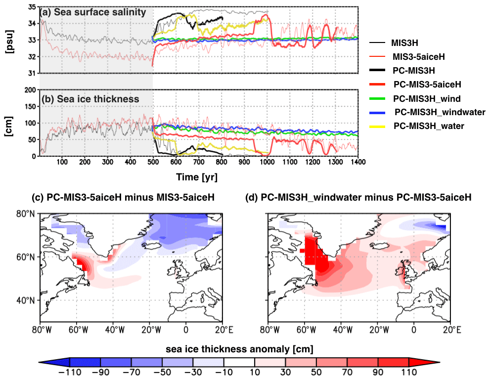
Figure 12Changes in sea surface conditions obtained from partially coupled experiments. Temporal evolution of February sea surface salinity (psu, a) and February sea ice thickness (cm, b) over the Irminger Sea (55–63∘ N, 35–25∘ W; left). Thin black: MIS3H, thin red: MIS3–5aiceH, thick black: PC-MIS3H, thick red: PC-MIS3–5aiceH, thick green: PC-MIS3Hwind, thick blue: PC-MIS3Hwindwater, thick yellow: PC-MIS3Hwater. Freshwater flux of 0.1 Sv is applied during years 0 to 500 (gray-shaded period). (c, d) Spatial maps of annual mean sea ice thickness (cm) averaged over years 501–600. Panel (c) shows the differences between a partially coupled experiment (PC-MIS3–5aiceH) and the corresponding original experiment (MIS3–5aiceH); panel (d) shows the effect of surface cooling by the MIS3 ice sheet (difference between PC-MIS3H_windwater and PC-MIS3–5aiceH). For panels (a) and (b), 11-year running means are shown.
Next, the effect of surface wind on the recovery time of the AMOC is explored. When the surface winds of the MIS5a ice sheet (MIS3–5aiceH) are applied to PC-MIS3H (PC-MIS3H_wind), the AMOC does not start to recover in the first 100 years, as seen in MIS3H (Fig. 11). This is related to the weaker cyclonic surface wind, which reduces the wind-driven oceanic transport of salt into the deepwater formation and caused a decrease of sea surface salinity there. Thus, partially coupled experiments show that the stronger wind in MIS3H creates favorable conditions to cause an earlier recovery of the AMOC. This is also confirmed by another sensitivity experiment showing earlier recovery of the AMOC when the surface wind of MIS3H is applied to PC-MIS3–5aiceH (not shown).
Interestingly, the AMOC does not recover in PC-MIS3H_wind during the integration, despite having the same surface wind forcing as in PC-MIS3–5aiceH, which recovers around year 900. A similar feature is also observed in PC-MIS3H_windwater (Table 2), where the model is forced with the surface cooling of the MIS3 ice sheet (MIS3H) and the surface wind and atmospheric freshwater flux of the MIS5a ice sheet (MIS3–5aiceH). The long stadial states observed in these two experiments are caused by the very thick sea ice over the deepwater formation region (green and blue lines compared to the red line in Fig. 12b, see also Fig. 12d), associated with stronger surface cooling by the MIS3 ice sheet (Fig. S5). After the cessation of freshwater hosing and the replacement of the surface wind, the sea surface salinity as well as the subsurface ocean temperature increase gradually in PC-MIS3H_wind and PC-MIS3H_windwater as in PC-MIS3–5aiceH. However, the thick sea ice over the deepwater region prevents the initiation of deepwater formation and maintains the weak AMOC (Loving and Vallis, 2005; Bitz et al., 2007; Oka et al., 2012; Sherriff-Tadano et al., 2021a). This result shows that the cooling effect of the MIS3 ice sheet plays a role in increasing the recovery time of the AMOC by increasing sea ice over the deepwater formation region.
Lastly, the effects of differences in atmospheric freshwater flux on the recovery time of the AMOC are explored for completeness. When the atmospheric freshwater flux of the MIS5a ice sheet (MIS3–5aiceH) is applied to PC-MIS3H (PC-MIS3H_water), the recovery time of the AMOC increases slightly (Fig. 11). This is associated with a decrease of sea surface salinity over the deepwater formation region (Fig. 12a), which is linked to the northward shift of the rain belt in the midlatitudes caused by the smaller ice sheet (Eisenman et al., 2009). Therefore, the larger MIS3 ice sheet reduces the recovery time of the AMOC by reducing the input of atmospheric freshwater flux over the deepwater formation region when compared to MIS5a ice sheet. Nevertheless, the differences in atmospheric freshwater flux have less impact on the duration of the recovery compared with the effect of wind in these experiments.
To summarize, the shorter recovery time in MIS3H compared with MIS3–5aiceH is a result of the dominance of the surface wind effect caused by larger ice sheets. The stronger cyclonic surface winds at mid-high latitudes in MIS3H than in MIS3–5aiceH (Fig. 10d) enhance the wind-driven transport of salt to the deepwater formation in MIS3H (Fig. 10e). In addition, the strong northerly wind anomaly over the western North Atlantic and the southward shift of westerly wind cause a reduction of wind-driven transport of sea ice to the deepwater formation region over Irminger Sea in MIS3H (Fig. 10f). The higher surface salinity (Fig. 8d) and thinner sea ice thickness (Fig. 8a) over the deepwater formation region during the weak AMOC state then increase the probability of the recovery of the AMOC and cause an early recovery in MIS3H (Fig. 3).
Our results show that the recovery time of the AMOC largely depends on the background climate. In MIS3H, the AMOC starts to recover soon after the cessation of freshwater hosing, whereas in MIS3–5aiceH, the AMOC first recovers gradually for several hundred years and then recovers abruptly (Fig. 3). From partially coupled experiments, it is found that the difference in surface wind plays a role in causing the shorter recovery of AMOC in MIS3H compared to MIS3–5aiceH (Fig. 11). In contrast, it is also found that the stronger surface cooling by larger ice sheets promote to increase in the recovery time of the AMOC by increasing the amount of sea ice over the deepwater formation region (Fig. 11). Thus, we find that the changes in the surface wind caused by the glacial ice sheet can contribute to a shorter stadial during MIS3 compared with MIS5, when its effect is stronger than that of surface cooling.
Previous studies show that the subsurface ocean temperature (Mignot et al., 2007; Gong et al., 2013), freshwater transport by the AMOC (de Vreis and Weber, 2005; Weber and Drijfhout, 2007; Liu et al., 2014) and surface winds (Goes et al., 2019) affect the recovery time of the AMOC. Our analysis of these parameters in hosing experiments shows results consistent with these studies. With respect to subsurface ocean temperature, the subsurface ocean temperature anomaly is larger in MIS3H than in MIS3–5aiceH, which favors early recovery of the AMOC by destabilizing the water column in the deepwater formation region (Gong et al., 2013). With respect to freshwater transport by the AMOC, our analysis shows a larger amount of freshwater transport into the Atlantic in MIS3H than in MIS3–5aiceH (0.073 and 0.017 Sv, respectively, before freshwater hosing). Thus, the results are also consistent with previous studies in that the experiment in which the AMOC transports more freshwater in the Atlantic recovers more quickly. Nevertheless, as shown in the partially coupled experiments, the AMOC cannot recover in PC-MIS3H_wind when the surface wind is weak over the deepwater formation region. With respect to wind forcing, Goes et al. (2019) show that the stronger surface wind in the LGM cause a shorter recovery time of the AMOC compared with that from the modern climate. Our study is also in line with their study in that the stronger surface wind in MIS3 compared with MIS5a induced by ice sheet differences causes a shorter recovery time of the AMOC. Therefore, together with Goes et al. (2019), this study reveals another important control on the recovery time of the AMOC: differences in localities of winds in the deepwater formation region. In this regard, this study supports the conclusion of Weber and Drijfhout (2007) and Bitz et al. (2007) that differences in atmospheric conditions play a role in controlling the recovery time of the AMOC.
Our findings can be used to interpret model discrepancies. Gong et al. (2013) show that the recovery time of the AMOC is shorter under mid-glacial and LGM conditions compared with the PI climate, whereas Weber and Drijhout (2007) and Bitz et al. (2007) show that the recovery time is longer under LGM conditions compared with PI conditions. In these studies, all of the boundary conditions (e.g., glacial ice sheets and CO2) are modified; thus, the reason for differences between the models remains elusive. Based on this study, we suggest that the wind effect of the glacial ice sheets plays the dominant role in the study of Gong et al. (2013), whereas the sea ice effect caused by lowering of the CO2 concentration and by the glacial ice sheet plays a larger role in the studies of Weber and Drijhout (2007) and Bitz et al. (2007). In fact, the surface winds are strongest in the mid-glacial experiment compared with the other experiments of Gong et al. (2013, 2015). In contrast, the surface winds are not stronger in the LGM simulations compared with the PI simulation by Bitz et al. (2007; Otto-Bliesner et al., 2006), even under the existence of glacial ice sheets. Although the cause of the difference in surface wind remains elusive, differences in the strength of the surface winds between models may cause the difference in the recovery time. Because Weber and Drihout (2007) use an EMIC, the model may underestimate the wind change caused by the glacial ice sheets. Therefore, the wind effect may not have a strong impact, and thus the sea ice effect will be played the dominant role.
Ice core studies recently suggest a possibility that the relation between the background climate and the durations of climate states can differ between interstadials and stadials; although the durations of both interstadials and stadials are generally affected by global temperatures and surface cooling (Buizert and Schmittner, 2015; Kawamura et al., 2017; Lohmann and Ditlevsen, 2019), the durations of stadials may be affected by additional conditions over the Northern Hemisphere (Lohmann, 2019) when the global climate is generally cold. A similar feature is also observed in climate model simulations of Sherriff-Tadano et al. (2021a) and this study. For example, using the same ice sheet forcing, Sherriff-Tadano et al. (2021a) show that differences in the vigorous AMOC between MIS5a and MIS3 are mainly caused by the differences in CO2. In their simulations, ice sheet differences have small impacts on the vigorous AMOC because of compensational balance between the strengthening effect of surface wind and the weakening effect of sea ice increase in the Northern Hemisphere and Southern Hemisphere. In contrast, in the hosing experiments of the present study, the effect of surface wind by the larger MIS3 ice sheets appears to be stronger compared with stronger surface cooling by the ice sheets and lower CO2, causing shortening of the stadials in MIS3 compared with MIS5a. These results support the findings of ice core studies and suggest that the relation between the background climate and the durations of climate states can differ between interstadials and stadials.
Although the expansion of glacial ice sheets from MIS5a to MIS3 can contribute to short stadials during the mid-glacial period, we should keep in mind that there are still large uncertainties in reconstructions of the glacial ice sheets prior to LGM. For example, sea level reconstructions show a wide range of ice sheet volume from 40 to 90 m sea level equivalent during MIS3 (Grant et al., 2012; Spratt and Lisiecki, 2016; Pico et al., 2017; Gowan et al., 2021). This can directly translate into uncertainties in the quantitative effect of the ice sheets on AMOC and can also indirectly affect the AMOC by changing the timing of the closure of Bering Strait, which may be important when interpreting DO cycles and AMOC variabilities (Hu et al., 2015). Furthermore, uncertainties in the shape of ice sheet may affect the balance of the surface wind and surface cooling effects on AMOC. Hence, further studies on similar topic using other ice sheet reconstructions are important to better interpret the evolution of millennial-timescale climate and AMOC variabilities over the glacial period.
There is also another unsolved problem: why are stadials very long during MIS2 and MIS4, when the glacial ice sheets are at their largest size (McManus et al., 1999; Buizert and Schmittner, 2015; Kawamura et al., 2017)? During these periods, summer insolation over the North Atlantic is very low; therefore, this may be important. In fact, Turney et al. (2015) show that lowering of the obliquity in MIS2 weakens the AMOC by increasing sea ice in the North Atlantic. In addition, very strong surface cooling by the glacial ice sheets may cause long stadials. In fact, we find that the strengthening of surface cooling by the larger ice sheets can increase the recovery time of the AMOC by increasing the amount of sea ice over the deepwater formation region. If there is a shift from a wind-dominated ice sheet effect, which shortens the recovery time of the AMOC, to a surface cooling-dominated ice sheet effect, the large ice sheets during MIS2 and MIS4 can contribute to the very long stadials. Further investigations of the roles of insolation and the ice sheet effect will be important for better understanding the glacial AMOC as well as interpreting the controlling parameters changing the duration of stadials over the glacial period.
Lastly, drastic weakening of the AMOC is induced by freshwater hosing in this study. Recent studies, however, show that the large-scale freshwater hosing is a result of weakening of the AMOC, rather than the cause of the drastic weakening of the AMOC (Alvarez-Solas et al., 2011; Barker et al., 2015). Nevertheless, the main point of our results is that once the AMOC is weakened by external forcing, the recovery time of the AMOC differs because of the ice sheet configurations. Thus, the external forcing that induces the weakening of the AMOC does not have to be a large discharge from the ice sheet and can be other forcing, such as a small amount of freshwater flux from the ice sheet, or perhaps volcanic eruptions. Hence, our results are applicable for DO cycles forced by external forcing. On the other hand, previous studies show that DO cycles may be excited by internal oscillation of the atmosphere–sea ice–ocean system (Arzel et al., 2010; Peltier and Vettoretti, 2014; Vettoretti and Peltier, 2016; Brown and Galbraith, 2016; Klockmann et al., 2018; Sherriff-Tadano and Abe-Ouchi, 2020). In Vettoretti and Peltier (2016) and Sherriff-Tadano and Abe-Ouchi (2020), the recovery of the AMOC is excited by the gradual warming of subsurface ocean and its balance with sea ice and surface salinity over deepwater formation region. From this point of view, the recovery process of the AMOC in the present hosing experiments is similar to that of the intrinsic oscillations of AMOC. Therefore, our findings may not be confined to the hosing experiments or DO cycles induced by external forcing but may also be applicable to DO cycles associated with intrinsic oscillations of AMOC. Hence, although we have not explicitly investigated the case of intrinsic oscillations of AMOC, we speculate that stronger winds in the northern North Atlantic can increase the probability of deepwater formation during stadials by modifying the balance of sea ice, surface salinity and subsurface ocean temperature. Nevertheless, it is important to assess our findings in this case as well.
To understand the reason why the durations of stadials are shorter during MIS3 compared with MIS5 despite the generally colder climate in MIS3, we explore the impact of the mid-glacial ice sheets on the durations of stadials. For this purpose, we conduct freshwater hosing experiments with the MIROC4m AOGCM under MIS3 and MIS5a conditions. Furthermore, to extract the impact of the difference in the glacial ice sheets on the recovery time of the AMOC, a sensitivity experiment is performed, which is forced with the MIS5a ice sheet under MIS3 CO2 and insolation conditions (MIS3–5aiceH). The ice sheets of MIS3 and MIS5a are taken from an ice sheet model, which reproduces the evolution of the ice sheets over the last 400 000 years (Abe-Ouchi et al., 2013). Freshwater hosing of 0.1 Sv over the northern North Atlantic induces collapse of the AMOC and southward expansion of sea ice, which covers the deepwater formation region in all experiments. After the cessation of freshwater hosing, the AMOC recovers in all experiments, which is associated with the initiation of deepwater formation in both the Irminger Sea and the Greenland Sea. However, the recovery time of the AMOC differs among the experiments; following the cessation of freshwater hosing, recovery starts after 80 years in MIS3, after approximately 200 years in MIS5a, and after approximately 600 years in MIS3–5aice. The slightly shorter recovery time in MIS3 compared with MIS5a is consistent with the ice core data. The sensitivity experiment (MIS3–5aiceH) extracting the effect of the mid-glacial ice sheet shows that a larger glacial ice sheet causes a shorter recovery time in MIS3, whereas lowering of the CO2 concentration and changes in insolation cause an increase of the recovery time. The partially coupled experiments further show that stronger surface winds over the North Atlantic shorten the recovery time by increasing the surface salinity and decreasing the sea ice amount in the deepwater formation region. In contrast, we also find that the surface cooling caused by larger ice sheets tends to increase the recovery time of the AMOC by increasing the sea ice thickness over the North Atlantic. In our simulation, the effect of surface winds appears to be stronger than the effect of surface cooling, thus causing a shortening of the recovery time of the AMOC. Therefore, our results suggest that the expansion of glacial ice sheets plays a role in reducing the duration of stadials during MIS3 and thus can contribute to the frequent DO cycles during MIS3 when the effect of surface winds dominates. Nevertheless, the effect of surface cooling may be important when the long stadials during the MIS2 and MIS4 and the model discrepancies are considered.
The MIROC code associated with this study is available to those who conduct collaborative research with the model users under license from copyright holders. The code of partially coupled experiments is available from the corresponding author (Sam Sherriff-Tadano) upon reasonable request. The simulation data are available from https://ccsr.aori.u-tokyo.ac.jp/~tadano/ (Sherriff-Tadano et al., 2021b).
The supplement related to this article is available online at: https://doi.org/10.5194/cp-17-1919-2021-supplement.
SST performed the climate model simulation and analyzed the results with the assistance of AAO and FS. SST performed the partially coupled experiments with the assistance of AO. SST and TM analyzed the ice core data. The manuscript was written by SST with contributions from AAO, AO, TM and FS.
The contact author has declared that neither they nor their co-authors have any competing interests.
Publisher’s note: Copernicus Publications remains neutral with regard to jurisdictional claims in published maps and institutional affiliations.
We thank Masahide Kimoto, Hiroyasu Hasumi, Masahiro Watanabe, Ryuji Tada, Masakazu Yoshimori and Takashi Obase for constructive discussion. The model simulations were performed on the Earth Simulator 3 at JAMSTEC. We thank Sara J. Mason for editing a draft of the manuscript. We would also like to thank the two reviewers and the editor, Laurie Menviel.
This research has been supported by the Japan Society for the Promotion of Science (grant nos. 15J12515, 17H06104, 17H06323, and 20K14552). Takahito Mitsui received funding by the Volkswagen Foundation.
This paper was edited by Laurie Menviel and reviewed by two anonymous referees.
Abe-Ouchi, A., Segawa, T., and Saito, F.: Climatic Conditions for modelling the Northern Hemisphere ice sheets throughout the ice age cycle, Clim. Past, 3, 423–438, https://doi.org/10.5194/cp-3-423-2007, 2007.
Abe-Ouchi, A., Saito, F., Kawamura, K., Raymo, M. E., Okuno, J., Takahashi, K., and Blatter, H.: Insolation-driven 100 000-year glacial cycles and hysteresis of ice-sheet volume, Nature, 500, 190–193, https://doi.org/10.1038/nature12374, 2013.
Álvarez-Solas, J., Montoya, M., Ritz, C., Ramstein, G., Charbit, S., Dumas, C., Nisancioglu, K., Dokken, T., and Ganopolski, A.: Heinrich event 1: an example of dynamical ice-sheet reaction to oceanic changes, Clim. Past, 7, 1297–1306, https://doi.org/10.5194/cp-7-1297-2011, 2011.
Arzel, O., de Verdiere, A. C., and England, M. H.: The Role of Oceanic Heat Transport and Wind Stress Forcing in Abrupt Millennial-Scale Climate Transitions, J. Climate, 23, 2233–2256, https://doi.org/10.1175/2009jcli3227.1, 2010.
Barker, S., Chen, J., Gong, X., Jonkers, L., Knorr, G., and Thornalley, D.: Icebergs not the trigger for North Atlantic cold events, Nature, 520, 333–336, https://doi.org/10.1038/nature14330, 2015.
Bereiter, B., Eggleston, S., Schmitt, J., Nehrbass-Ahles, C., Stocker, T. F., Fischer, H., Kipfstuhl, S., and Chappellaz, J.: Revision of the EPICA Dome C CO2 record from 800 to 600 kyr before present, Geophys. Res. Lett., 42, 542–549, https://doi.org/10.1002/2014gl061957, 2015.
Bitz, C. M., Chiang, J. C. H., Cheng, W., and Barsugli, J. J.: Rates of thermohaline recovery from freshwater pulses in modern, Last Glacial Maximum, and greenhouse warming climates, Geophys. Res. Lett., 34, L07708, https://doi.org/10.1029/2006gl029237, 2007.
Boers, N.: Early-warning signals for Dansgaard-Oeschger events in a high-resolution ice core record, Nat. Comm. 9, 2556, https://doi.org/10.1038/s41467-018-04881-7, 2018.
Bohm, E., Lippold, J., Gutjahr, M., Frank, M., Blaser, P., Antz, B., Fohlmeister, J., Frank, N., Andersen, M. B., and Deininger, M.: Strong and deep Atlantic meridional overturning circulation during the last glacial cycle, Nature, 517, 73–170, https://doi.org/10.1038/nature14059, 2015.
Brady, E. C., Otto-Bliesner, B. L., Kay, J. E., and Rosenbloom, N.: Sensitivity to Glacial Forcing in the CCSM4, J. Climate, 26, 1901–1925, https://doi.org/10.1175/jcli-d-11-00416.1, 2013.
Brown, N. and Galbraith, E. D.: Hosed vs. unhosed: interruptions of the Atlantic Meridional Overturning Circulation in a global coupled model, with and without freshwater forcing, Clim. Past, 12, 1663–1679, https://doi.org/10.5194/cp-12-1663-2016, 2016.
Buizert, C. and Schmittner, A.: Southern Ocean control of glacial AMOC stability and Dansgaard-Oeschger interstadial duration, Paleoceanography, 30, 1595–1612, https://doi.org/10.1002/2015pa002795, 2015.
Capron, E., Landais, A., Chappellaz, J., Schilt, A., Buiron, D., Dahl-Jensen, D., Johnsen, S. J., Jouzel, J., Lemieux-Dudon, B., Loulergue, L., Leuenberger, M., Masson-Delmotte, V., Meyer, H., Oerter, H., and Stenni, B.: Millennial and sub-millennial scale climatic variations recorded in polar ice cores over the last glacial period, Clim. Past, 6, 345–365, https://doi.org/10.5194/cp-6-345-2010, 2010.
Chan, W.-L. and Abe-Ouchi, A.: Pliocene Model Intercomparison Project (PlioMIP2) simulations using the Model for Interdisciplinary Research on Climate (MIROC4m), Clim. Past, 16, 1523–1545, https://doi.org/10.5194/cp-16-1523-2020, 2020.
Chan, W.-L., Abe-Ouchi, A., and Ohgaito, R.: Simulating the mid-Pliocene climate with the MIROC general circulation model: experimental design and initial results, Geosci. Model Dev., 4, 1035–1049, https://doi.org/10.5194/gmd-4-1035-2011, 2011.
Dallenbach, A., Blunier, T., Fluckiger, J., Stauffer, B., Chappellaz, J., and Raynaud, D.: Changes in the atmospheric CH4 gradient between Greenland and Antarctica during the Last Glacial and the transition to the Holocene, Geophys. Res. Lett., 27, 1005–1008, https://doi.org/10.1029/1999gl010873, 2000.
Dansgaard, W., Johnsen, S. J., Clausen, H. B., Dahljensen, D., Gundestrup, N. S., Hammer, C. U., Hvidberg, C. S., Steffensen, J. P., Sveinbjornsdottir, A. E., Jouzel, J., and Bond, G.: Evidence for general instability of past climate from a 250 kyr ice-core record, Nature, 364, 218–220, https://doi.org/10.1038/364218a0, 1993.
Deplazes, G., Lückge, A., Stuut, J.-B. W., Pätzold, J., Kuhlmann, H., Husson, D., Fant, M., and Haug, G. H.: Weakening and strengthening of the Indian monsoon during Heinrich events and Dansgaard-Oeschger oscillations, Paleoceanography, 29, 99–114, https://doi.org/10.1002/2013PA002509, 2014.
de Vries, P. and Weber, S. L.: The Atlantic freshwater budget as a diagnostic for the existence of a stable shut down of the meridional overturning circulation, Geophys. Res. Lett., 32, L09606, https://doi.org/10.1029/2004gl021450, 2005.
Dokken, T. M., Nisancioglu, K. H., Li, C., Battisti, D. S., and Kissel, C.: Dansgaard-Oeschger cycles: Interactions between ocean and sea ice intrinsic to the Nordic seas, Paleoceanography, 28, 491–502, https://doi.org/10.1002/palo.20042, 2013.
Eisenman, I., Bitz, C. M., and Tziperman, E.: Rain driven by receding ice sheets as a cause of past climate change, Paleoceanography, 24, PA4209, https://doi.org/10.1029/2009pa001778, 2009.
Galbraith, E. and de Lavergne, C.: Response of a comprehensive climate model to a broad range of external forcings: relevance for deep ocean ventilation and the development of late Cenozoic ice ages, Clim. Dynam., 52, 653–679, https://doi.org/10.1007/s00382-018-4157-8, 2019.
Ganopolski, A. and Rahmstorf, S.: Rapid changes of glacial climate simulated in a coupled climate model, Nature, 409, 153–158, https://doi.org/10.1038/35051500, 2001.
Goes, M., Murphy, L. N., and Clement, A. C.: The Stability of the AMOC During Heinrich Events Is Not Dependent on the AMOC Strength in an Intermediate Complexity Earth System Model Ensemble, Paleoceanography and Paleoclimatology, 34, 1359–1374, https://doi.org/10.1029/2019pa003580, 2019.
Gong, X., Knorr, G., Lohmann, G., and Zhang, X.: Dependence of abrupt Atlantic meridional ocean circulation changes on climate background states, Geophys. Res. Lett., 40, 3698–3704, https://doi.org/10.1002/grl.50701, 2013.
Gong, X., Zhang, X. D., Lohmann, G., Wei, W., Zhang, X., and Pfeiffer, M.: Higher Laurentide and Greenland ice sheets strengthen the North Atlantic ocean circulation, Clim. Dynam., 45, 139–150, https://doi.org/10.1007/s00382-015-2502-8, 2015.
Gowan, E. J., Zhang, X., Khosravi, S., Rovere, A., Stocchi, P., Hughes, A. L. C., Gyllencreutz, R., Mangerud, J., Svendsen, J. I., and Lohmann, G.: A new global ice sheet reconstruction for the past 80000 years, Nat. Commun., 12, 1199, https://doi.org/10.1038/s41467-021-21469-w, 2021.
Grant, K. M., Rohling, E. J., Bar-Matthews, M., Ayalon, A., Medina-Elizalde, M., Ramsey, C. B., Satow, C., and Roberts, A. P.: Rapid coupling between ice volume and polar temperature over the past 150 000 years, Nature, 491, 744–747, https://doi.org/10.1038/nature11593, 2012.
Gregory, J. M., Dixon, K. W., Stouffer, R. J., Weaver, A. J., Driesschaert, E., Eby, M., Fichefet, T., Hasumi, H., Hu, A., Jungclaus, J. H., Kamenkovich, I. V., Levermann, A., Montoya, M., Murakami, S., Nawrath, S., Oka, A., Sokolov, A. P., and Thorpe, R. B.: A model intercomparison of changes in the Atlantic thermohaline circulation in response to increasing atmospheric CO2 concentration, Geophys. Res. Lett., 32, L12703, https://doi.org/10.1029/2005gl023209, 2005.
Guo, C., Nisancioglu, K. H., Bentsen, M., Bethke, I., and Zhang, Z.: Equilibrium simulations of Marine Isotope Stage 3 climate, Clim. Past, 15, 1133–1151, https://doi.org/10.5194/cp-15-1133-2019, 2019.
Hasumi, H. and Emori, S.: K-1 coupled model (MIROC) description, K-1 Technical Report 1, Center For Climate System Research, Univ. of Tokyo, Tokyo, Japan, 34 pp., 2004.
Henry, L. G., McManus, J. F., Curry, W. B., Roberts, N. L., Piotrowski, A. M., and Keigwin, L. D.: North Atlantic ocean circulation and abrupt climate change during the last glaciation, Science, 353, 470–474, https://doi.org/10.1126/science.aaf5529, 2016.
Hu, A. X., Meehl, G. A., Han, W. Q., Otto-Bliestner, B., Abe-Ouchi, A., and Rosenbloom, N.: Effects of the Bering Strait closure on AMOC and global climate under different background climates, Prog. Oceanogr., 132, 174–196, https://doi.org/10.1016/j.pocean.2014.02.004, 2015.
Huber, C., Leuenberger, M., Spahni, R., Fluckiger, J., Schwander, J., Stocker, T. F., Johnsen, S., Landals, A., and Jouzel, J.: Isotope calibrated Greenland temperature record over Marine Isotope Stage 3 and its relation to CH4, Earth Planet. Sc. Lett., 243, 504–519, https://doi.org/10.1016/j.epsl.2006.01.002, 2006.
Kageyama, M., Paul, A., Roche, D. M., and Van Meerbeeck, C. J.: Modelling glacial climatic millennial-scale variability related to changes in the Atlantic meridional overturning circulation: a review, Quaternary Sci. Rev., 29, 2931–2956, https://doi.org/10.1016/j.quascirev.2010.05.029, 2010.
Kageyama, M., Merkel, U., Otto-Bliesner, B., Prange, M., Abe-Ouchi, A., Lohmann, G., Ohgaito, R., Roche, D. M., Singarayer, J., Swingedouw, D., and X Zhang: Climatic impacts of fresh water hosing under Last Glacial Maximum conditions: a multi-model study, Clim. Past, 9, 935–953, https://doi.org/10.5194/cp-9-935-2013, 2013.
Kawamura, K., Abe-Ouchi, A., Motoyama, H., Ageta, Y., Aoki, S., Azuma, N., Fujii, Y., Fujita, K., Fujita, S., Fukui, K., Furukawa, T., Furusaki, A., Goto-Azuma, K., Greve, R., Hirabayashi, M., Hondoh, T., Hori, A., Horikawa, S., Horiuchi, K., Igarashi, M., Iizuka, Y., Kameda, T., Kanda, H., Kohno, M., Kuramoto, T., Matsushi, Y., Miyahara, M., Miyake, T., Miyamoto, A., Nagashima, Y., Nakayama, Y., Nakazawa, T., Nakazawa, F., Nishio, F., Obinata, I., Ohgaito, R., Oka, A., Okuno, J., Okuyama, J., Oyabu, I., Parrenin, F., Pattyn, F., Saito, F., Saito, T., Saito, T., Sakurai, T., Sasa, K., Seddik, H., Shibata, Y., Shinbori, K., Suzuki, K., Suzuki, T., Takahashi, A., Takahashi, K., Takahashi, S., Takata, M., Tanaka, Y., Uemura, R., Watanabe, G., Watanabe, O., Yamasaki, T., Yokoyama, K., Yoshimori, M., and Yoshimoto, T.: State dependence of climatic instability over the past 720 000 years from Antarctic ice cores and climate modeling, Sci. Adv., 3, e1600446, https://doi.org/10.1126/sciadv.1600446, 2017.
Kindler, P., Guillevic, M., Baumgartner, M., Schwander, J., Landais, A., and Leuenberger, M.: Temperature reconstruction from 10 to 120 kyr b2k from the NGRIP ice core, Clim. Past, 10, 887–902, https://doi.org/10.5194/cp-10-887-2014, 2014.
Kleppin, H., Jochum, M., Otto-Bliesner, B., Shields, C. A., and Yeager, S.: Stochastic Atmospheric Forcing as a Cause of Greenland Climate Transitions, J. Climate, 28, 7741–7763, https://doi.org/10.1175/jcli-d-14-00728.1, 2015.
Klockmann, M., Mikolajewicz, U., and Marotzke, J.: The effect of greenhouse gas concentrations and ice sheets on the glacial AMOC in a coupled climate model, Clim. Past, 12, 1829–1846, https://doi.org/10.5194/cp-12-1829-2016, 2016.
Klockmann, M., Mikolajewicz, U., and Marotzke, J.: Two AMOC states in response to decreasing greenhouse gas concentrations in the coupled climate model MPI-ESM, J. Climate, 31, 7969–7984, https://doi.org/10.1175/JCLI-D-17-0859.1, 2018.
Liu, W., Liu, Z., and Brady, E. C.: Why is the AMOC Monostable in Coupled General Circulation Models?, J. Climate, 27, 2427–2443, https://doi.org/10.1175/jcli-d-13-00264.1, 2014.
Lohmann, J.: Prediction of Dansgaard-Oeschger Events From Greenland Dust Records, Geophys. Res. Lett., 46, 12427–12434, https://doi.org/10.1029/2019gl085133, 2019.
Lohmann, J. and Ditlevsen, P. D.: Objective extraction and analysis of statistical features of Dansgaard–Oeschger events, Clim. Past, 15, 1771–1792, https://doi.org/10.5194/cp-15-1771-2019, 2019.
Loving, J. L. and Vallis, G. K.: Mechanisms for climate variability during glacial and interglacial periods, Paleoceanography, 20, PA4024, https://doi.org/10.1029/2004pa001113, 2005.
Marotzke, J.: CLIMATE SCIENCE A grip on ice-age ocean circulation, Nature, 485, 180–181, https://doi.org/10.1038/485180a, 2012.
McManus, J. F., Oppo, D. W., and Cullen, J. L.: A 0.5-million-year record of millennial-scale climate variability in the North Atlantic, Science, 283, 971–975, https://doi.org/10.1126/science.283.5404.971, 1999.
Menviel, L., Timmermann, A., Friedrich, T., and England, M. H.: Hindcasting the continuum of Dansgaard–Oeschger variability: mechanisms, patterns and timing, Clim. Past, 10, 63–77, https://doi.org/10.5194/cp-10-63-2014, 2014.
Menviel, L. C., Skinner, L. C., Tarasov, L., and Tzedakis, P. C.: An ice–climate oscillatory framework for Dansgaard–Oeschger cycles, Nat. Rev. Earth Environ., 1, 677–693, https://doi.org/10.1038/s43017-020-00106-y, 2020.
Mignot, J., Ganopolski, A., and Levermann, A.: Atlantic subsurface temperatures: Response to a shutdown of the overturning circulation and consequences for its recovery, J. Climate, 20, 4884–4898, https://doi.org/10.1175/jcli4280.1, 2007.
Mikolajewicz, U. and Voss, R.: The role of the individual air-sea flux components in CO2-induced changes of the ocean's circulation and climate, Clim. Dynam., 16, 627–642, https://doi.org/10.1007/s003820000066, 2000.
Mitsui, T. and Crucifix, M.: Influence of external forcings on abrupt millennial-scale climate changes: a statistical modelling study, Clim. Dynam., 48, 2729–2749, https://doi.org/10.1007/s00382-016-3235-z, 2017.
Montoya, M. and Levermann, A.: Surface wind-stress threshold for glacial Atlantic overturning, Geophys. Res. Lett., 35, L03608, https://doi.org/10.1029/2007gl032560, 2008.
Muglia, J. and Schmittner, A.: Glacial Atlantic overturning increased by wind stress in climate models, Geophys. Res. Lett., 42, 9862–9869, https://doi.org/10.1002/2015gl064583, 2015.
Obase, T. and Abe-Ouchi, A.: Abrupt Bolling-Allerod Warming Simulated under Gradual Forcing of the Last Deglaciation, Geophys. Res. Lett., 46, 11397–11405, https://doi.org/10.1029/2019gl084675, 2019.
O'ishi, R., Chan, W.-L., Abe-Ouchi, A., Sherriff-Tadano, S., Ohgaito, R., and Yoshimori, M.: PMIP4/CMIP6 last interglacial simulations using three different versions of MIROC: importance of vegetation, Clim. Past, 17, 21–36, https://doi.org/10.5194/cp-17-21-2021, 2021.
Oka, A., Hasumi, H., Okada, N., Sakamoto, T. T., and Suzuki, T.: Deep convection seesaw controlled by freshwater transport through the Denmark Strait, Ocean Model., 15, 157–176, https://doi.org/10.1016/j.ocemod.2006.08.004, 2006.
Oka, A., Hasumi, H., and Abe-Ouchi, A.: The thermal threshold of the Atlantic meridional overturning circulation and its control by wind stress forcing during glacial climate, Geophys. Res. Lett., 39, L09709, https://doi.org/10.1029/2012GL051421, 2012.
Oka, A., Abe-Ouchi, A., Sherriff-Tadano, S., Yokoyama, Y., Kawamura, K., and Hasumi, H.: Glacial mode shift of the Atlantic meridional overturning circulation by warming over the Southern Ocean, Commun. Earth Environ., 2, 169, https://doi.org/10.1038/s43247-021-00226-3, 2021.
Otto-Bliesner, B. L., Brady, E. C., Clauzet, G., Tomas, R., Levis, S., and Kothavala, Z.: Last Glacial Maximum and Holocene climate in CCSM3, J. Climate, 19, 2526–2544, https://doi.org/10.1175/jcli3748.1, 2006.
Pausata, F. S. R., Li, C., Wettstein, J. J., Kageyama, M., and Nisancioglu, K. H.: The key role of topography in altering North Atlantic atmospheric circulation during the last glacial period, Clim. Past, 7, 1089–1101, https://doi.org/10.5194/cp-7-1089-2011, 2011.
Peltier, W. R. and Vettoretti, G.: Dansgaard-Oeschger oscillations predicted in a comprehensive model of glacial climate: A “kicked” salt oscillator in the Atlantic, Geophys. Res. Lett., 41, 7306–7313, https://doi.org/10.1002/2014gl061413, 2014.
Pico, T., Creveling, J. R., and Mitrovica, J. X.: Sea-level records from the US mid-Atlantic constrain Laurentide Ice Sheet extent during Marine Isotope Stage 3, Nat. Commun., 8, 15612, https://doi.org/10.1038/ncomms15612, 2017.
Piotrowski, A. M., Goldstein, S. L., Hemming, S. R., and Fairbanks, R. G.: Temporal relationships of carbon cycling and ocean circulation at glacial boundaries, Science, 307, 1933–1938, https://doi.org/10.1126/science.1104883, 2005.
Rasmussen, S. O., Bigler, M., Blockley, S. P., Blunier, T., Buchardt, S. L., Clausen, H. B., Cvijanovic, I., Dahl-Jensen, D., Johnsen, S. J., Fischer, H., Gkinis, V., Guillevic, M., Hoek, W. Z., Lowe, J. J., Pedro, J. B., Popp, T., Seierstad, I. K., Steffensen, J. P., Svensson, A. M., Vallelonga, P., Vinther, B. M., Walker, M. J. C., Wheatley, J. J., and Winstrup, M.: A stratigraphic framework for abrupt climatic changes during the Last Glacial period based on three synchronized Greenland ice-core records: refining and extending the INTIMATE event stratigraphy, Quaternary Sci. Rev., 106, 14–28, https://doi.org/10.1016/j.quascirev.2014.09.007, 2014.
Rasmussen, T. L. and Thomsen, E.: The role of the North Atlantic Drift in the millennial timescale glacial climate fluctuations, Palaeogeography Palaeoclimatology Palaeoecology, 210, 101–116, https://doi.org/10.1016/j.palaeo.2004.04.005, 2004.
Renold, M., Raible, C. C., Yoshimori, M., and Stocker, T. F.: Simulated resumption of the North Atlantic meridional overturning circulation – Slow basin-wide advection and abrupt local convection, Quaternary Sci. Rev., 29, 101–112, https://doi.org/10.1016/j.quascirev.2009.11.005, 2010.
Sadatzki, H., Dokken, T. M., Berben, S. M. P., Muschitiello, F., Stein, R., Fahl, K., Menviel, L., Timmermann, A., and Jansen, E.: Sea ice variability in the southern Norwegian Sea during glacial Dansgaard-Oeschger climate cycles, Sci. Adv., 5, eaau6174, https://doi.org/10.1126/sciadv.aau6174, 2019.
Schmittner, A., Meissner, K. J., Eby, M., and Weaver, A. J.: Forcing of the deep ocean circulation in simulations of the Last Glacial Maximum, Paleoceanography, 17, 1015, https://doi.org/10.1029/2001pa000633, 2002.
Sherriff-Tadano, S. and Abe-Ouchi, A.: Roles of sea ice–surface wind feedback in maintaining the glacial Atlantic meridional overturning circulation and climate, J. Climate, 33, 3001–3018, https://doi.org/10.1175/JCLI-D-19-0431.1, 2020.
Sherriff-Tadano, S., Abe-Ouchi, A., Yoshimori, M., Oka, A., and Chan, W.-L.: Influence of glacial ice sheets on the Atlantic meridional overturning circulation through surface wind change, Clim. Dynam., 50, 2881–2903, https://doi.org/10.1007/s00382-017-3780-0, 2018.
Sherriff-Tadano, S., Abe-Ouchi, A., and Oka, A.: Impact of mid-glacial ice sheets on deep ocean circulation and global climate, Clim. Past, 17, 95–110, https://doi.org/10.5194/cp-17-95-2021, 2021a.
Sherriff-Tadano, S., Abe-Ouchi, A., Oka, A., Mitsui, T., and Saito, F.: Data repository, [data set], available at: https://ccsr.aori.u-tokyo.ac.jp/~tadano/, last access: 18 September 2021b.
Smith, R. S. and Gregory, J.: The last glacial cycle: transient simulations with an AOGCM, Clim. Dynam., 38, 1545–1559, https://doi.org/10.1007/s00382-011-1283-y, 2012.
Spratt, R. M. and Lisiecki, L. E.: A Late Pleistocene sea level stack, Clim. Past, 12, 1079–1092, https://doi.org/10.5194/cp-12-1079-2016, 2016.
Turney, C. S. M., Thomas, Z. A., Hutchinson, D. K., Bradshaw, C. J. A., Brook, B. W., England, M. H., Fogwill, C. J., Jones, R. T., Palmer, J., Hughen, K. A., and Cooper, A.: Obliquity-driven expansion of North Atlantic sea ice during the last glacial, Geophys. Res. Lett., 42, 10382–10390, https://doi.org/10.1002/2015gl066344, 2015.
Vettoretti, G. and Peltier, W. R.: Thermohaline instability and the formation of glacial North Atlantic super polynyas at the onset of Dansgaard-Oeschger warming events, Geophys. Res. Lett., 43, 5336–5344, https://doi.org/10.1002/2016gl068891, 2016.
Wang, X., Auler, A., Edwards, R., Cheng, H., Cristalli, P. S., Smart, P. L., Richards, D. A., and Shen, C.-C.: Wet periods in northeastern Brazil over the past 210 kyr linked to distant climate anomalies, Nature, 432, 740–743, https://doi.org/10.1038/nature03067, 2004.
Weber, S. L. and Drijfhout, S. S.: Stability of the Atlantic meridional overturning circulation in the last glacial maximum climate, Geophys. Res. Lett., 34, L22706, https://doi.org/10.1029/2007gl031437, 2007.
Yamamoto, A., Abe-Ouchi, A., Shigemitsu, M., Oka, A., Takahashi, K., Ohgaito, R., and Yamanaka, Y.: Global deep ocean oxygenation by enhanced ventilation in the Southern Ocean under long-term global warming, Global Biogeochem. Cy., 29, 1801–1815, https://doi.org/10.1002/2015gb005181, 2015.
Zhang, X., Lohmann, G., Knorr, G., and Purcell, C.: Abrupt glacial climate shifts controlled by ice sheet changes, Nature, 512, 290–294, 30 2014a.
Zhang, X., Prange, M., Merkel, U., and Schulz, M.: Instability of the Atlantic overturning circulation during Marine Isotope Stage 3, Geophys. Res. Lett., 41, 4285–4293, https://doi.org/10.1002/2014GL060321, 2014b.