the Creative Commons Attribution 4.0 License.
the Creative Commons Attribution 4.0 License.
 | 17 Sep 2021
Enhanced moisture delivery into Victoria Land, East Antarctica, during the early Last Interglacial: implications for West Antarctic Ice Sheet stability
Nicole E. Spaulding
Michael L. Bender
Edward J. Brook
John A. Higgins
Andrei V. Kurbatov
Paul A. Mayewski
The S27 ice core, drilled in the Allan Hills Blue Ice Area of East Antarctica, is located in southern Victoria Land, ∼80 km away from the present-day northern edge of the Ross Ice Shelf. Here, we utilize the reconstructed accumulation rate of S27 covering the Last Interglacial (LIG) period between 129 ka and 116 ka (where ka indicates thousands of years before present) to infer moisture transport into the region. The accumulation rate is based on the ice-age–gas-age differences calculated from the ice chronology, which is constrained by the stable water isotopes of the ice, and an improved gas chronology based on measurements of oxygen isotopes of O2 in the trapped gases. The peak accumulation rate in S27 occurred at 128.2 ka, near the peak LIG warming in Antarctica. Even the most conservative estimate yields an order-of-magnitude increase in the accumulation rate during the LIG maximum, whereas other Antarctic ice cores are typically characterized by a glacial–interglacial difference of a factor of 2 to 3. While part of the increase in S27 accumulation rates must originate from changes in the large-scale atmospheric circulation, additional mechanisms are needed to explain the large changes. We hypothesize that the exceptionally high snow accumulation recorded in S27 reflects open-ocean conditions in the Ross Sea, created by reduced sea ice extent and increased polynya size and perhaps by a southward retreat of the Ross Ice Shelf relative to its present-day position near the onset of the LIG. The proposed ice shelf retreat would also be compatible with a sea-level high stand around 129 ka significantly sourced from West Antarctica. The peak in S27 accumulation rates is transient, suggesting that if the Ross Ice Shelf had indeed retreated during the early LIG, it would have re-advanced by 125 ka.
- Article
(4810 KB) - Full-text XML
-
Supplement
(4937 KB) - BibTeX
- EndNote


The West Antarctic Ice Sheet (WAIS) is grounded on bedrock that currently lies below sea level and is therefore vulnerable to rising temperatures (Mercer, 1968; Hughes, 1973). Yet, the stability of the WAIS remains poorly understood and constitutes a major source of uncertainty in projecting future sea-level rises in a warming world (Dutton et al., 2015a; DeConto and Pollard, 2016). One way to constrain the sensitivity of ice sheets to climate change is to explore their behavior during past warm periods. The Last Interglacial (LIG) between 129 ka and 116 ka (where ka indicates thousands of years before present) is a geologically recent warm interval with an average global temperature 0 to 2 ∘C above the pre-industrial level (Otto-Bliesner et al., 2013). The LIG could therefore shed light on the response of the WAIS to future warming. While the WAIS must have contributed to the LIG sea-level high stand (Dutton et al., 2015a, and references therein), quantifying these contributions is challenging and the timing of such WAIS changes (early versus late in LIG) is still debated (e.g., Yau et al., 2016; Rohling et al., 2019; Clark et al., 2020).
As the floating extension of land ice masses, the extent of sea ice and ice shelves can provide important insights into the dynamics of continental ice sheets. For example, as the ocean warms and sea level rises, the loss of ice shelves due to calving and basal melting may lead to further losses of the continental ice they buttress (Pritchard et al., 2012). The Ross Ice Shelf (RIS) is the largest ice shelf in Antarctica, located between Marie Byrd Land in West Antarctica and Victoria Land in East Antarctica (Fig. 1). Ice sheet models have suggested that the complete disintegration of the Ross Ice Shelf may have accompanied the collapse of the WAIS in both past and future simulations (DeConto and Pollard, 2016; Garbe et al., 2020). However, terrestrial evidence is lacking due to subsequent ice sheet growth, and existing marine records do not have enough temporal resolution to resolve the extent of RIS during the LIG.
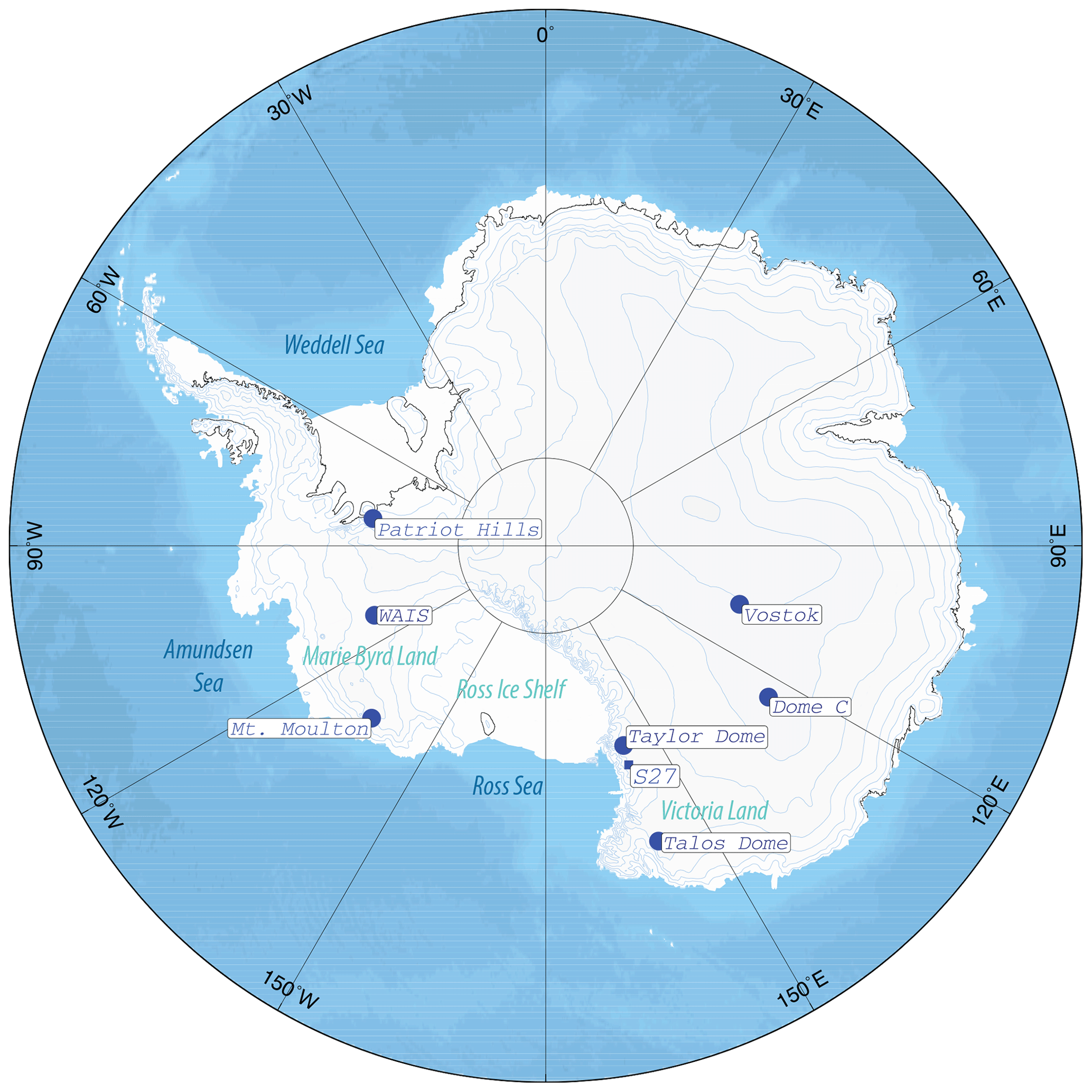
Figure 1Locations of key ice coring sites and geographic features of Antarctica. The rectangle indicates the location of Site 27 (S27). Other ice coring sites mentioned in this study are marked with blue circles (map source: Bindschadler et al., 2011).
Ice cores provide continuous, well-dated records of local climate information that is, in turn, sensitive to the extent of nearby ice masses. The position of the ice margin and sea ice extent can impact atmospheric circulation, snow deposition, and isotopic signatures in the precipitation captured in ice cores (Morse et al., 1998; Steig et al., 2015; Holloway et al., 2016). In this study, we use a shallow ice core – Site 27 (S27) from the Allan Hills Blue Ice Area (BIA) – to explore RIS changes during the LIG. The Allan Hills BIA in Victoria Land, East Antarctica, is ideally located near the present-day northwest margin of the RIS (Figs. 1 and S1 in the Supplement). S27 provides a continuous climate record between 115 and 255 ka (Spaulding et al., 2013). The close proximity of Site 27 to the Ross Sea embayment holds the potential to shed light on the behavior of the Ross Ice Shelf during Termination II (the transition from the Penultimate Glacial Maximum to the LIG) and, by extension, on the West Antarctic Ice Sheet.
Here, we present a record of the accumulation rate of Site 27 between 115 and 140 ka, derived from independently constrained ice and gas chronologies. This approach has previously been applied to Taylor Glacier blue ice samples to estimate accumulation rates between 10 and 40 ka (Baggenstos et al., 2018) and between 55 and 84 ka (Menking et al., 2019). We take advantage of the fact that the age of the ice is older than the age of the trapped gases at the same depth. This age difference (Δage) results from the process of converting snow into ice (firn densification) and reflects the age of the ice when the firn crosses a threshold density where the gases become isolated in impermeable ice. The evolution of firn density is found to empirically correlate with the ice accumulation rate and surface temperature (Herron and Langway, 1980). Subsequent ice thinning and flow do not alter this Δage.
The ice chronology of S27 was originally established by matching features in the stable water isotopes (δDice) to those in the EPICA Dome C (EDC) record (Fig. 2; Spaulding et al., 2013). The δ notation here is defined as ‰, where R is the raw ratio. Similarities between S27 and EDC δDice overall give us confidence in the stratigraphic continuity of the S27 ice core. By contrast, a preliminary gas age timescale is available in Spaulding et al. (2013), constructed by matching the δ18O of atmospheric O2 (δ18Oatm) measured in S27 (sample N=39) to the δ18Oatm record of the Vostok ice core (Fig. S2 in the Supplement). This preliminary δ18Oatm record, however, did not capture a δ18Oatm peak between 170 and 190 ka because either the measurement is too sparse or the S27 ice core might not be continuous after all. We note, however, that δDice in this interval aligns well with the δDice record at Vostok, supporting the continuity of the S27 core.
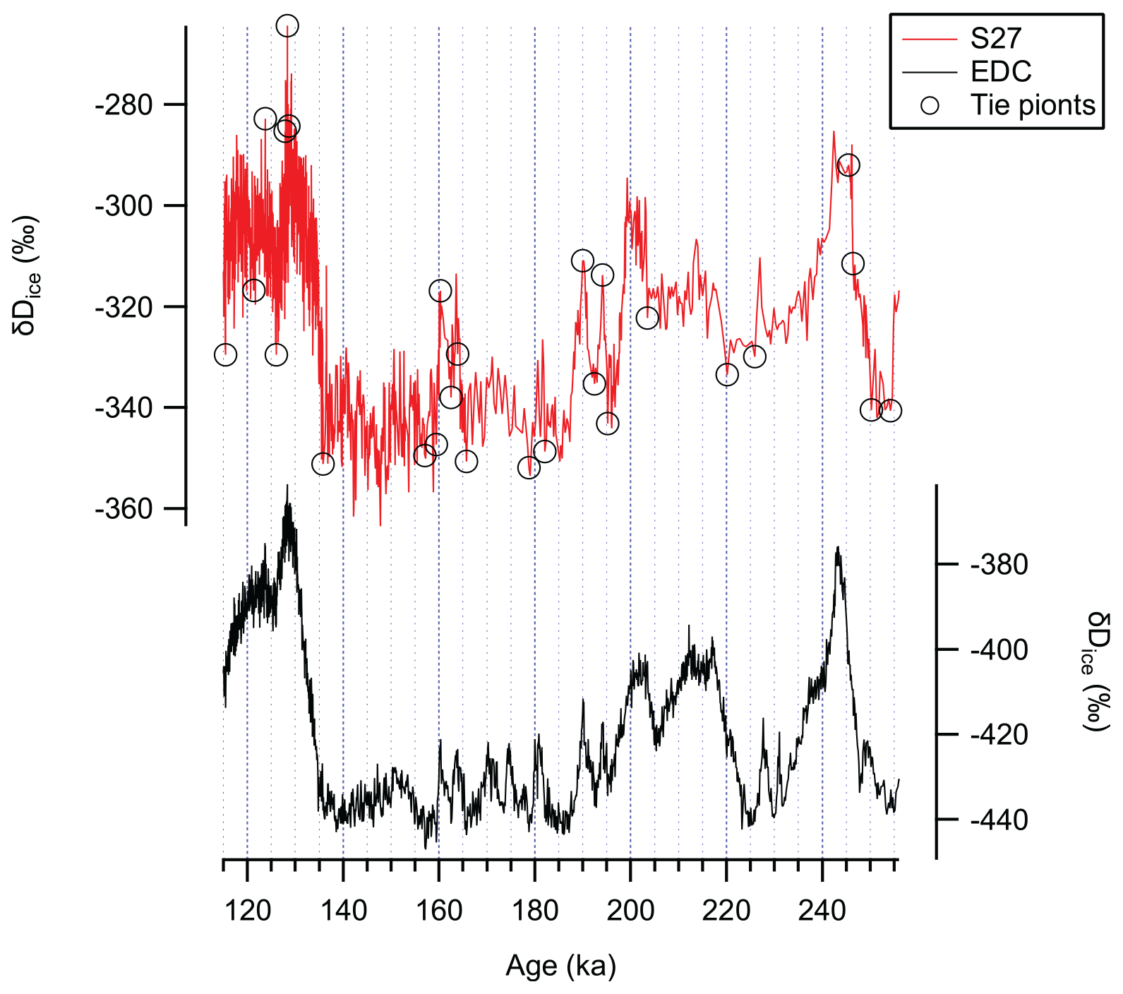
Figure 2Stable water isotope records in S27 (red; Spaulding et al., 2013) and EDC (black; Jouzel et al., 2007) between 115 and 255 ka. Tie points in S27 δDice used by Spaulding et al. (2013) are marked as circles.
In this study, we extend the existing S27 δ18Oatm measurements by adding new δ18Oatm values at 45 depths, including one that overlaps with earlier data, in order to understand the stratigraphic integrity of the record at ∼180 ka and further improve the gas chronology. This collated δ18Oatm record is then correlated with a recently published δ18Oatm record of EDC (Extier et al., 2018) to derive a more accurate and complete gas chronology for S27. New measurements of CH4 and CO2 from the S27 ice core are also used to further improve the δ18Oatm-based age scale between 105 and 147 ka. The gas chronology developed here, together with the ice chronology reported in Spaulding et al. (2013), yields the Δage, from which the accumulation rate at Site 27 is estimated. We then examine the accumulation rate history in the context of atmospheric circulation changes and ice shelf and/or ice sheet stability during the LIG.
2.1 Glaciological setting
The Site 27 (S27; 76.70∘ S, 159.31∘ E) ice core was drilled along the main ice flow line (MIF; Spaulding et al., 2012) of the Allan Hills region. It is situated to the northwest of the Convoy Range and the McMurdo Dry Valleys in southern Victoria Land, East Antarctica, about 80 km from the Ross Sea coastline (Figs. 1 and S1). MIF ice flows slowly (<0.5 m yr−1) from the southwest to the northeast and feeds into the Mawson Glacier before eventually draining into the Ross Sea embayment. Horizontal ice velocities decrease as the ice approaches the Allan Hills nunatak: from 0.4–0.5 m yr−1 in the upstream portion of the MIF to less than 0.3 m yr−1 near where S27 is located, with the slowest ice flow rate in the area being 0.015 m yr−1 (Spaulding et al., 2012).
The accumulation area of the ice feeding the Allan Hills BIA today lies about 20 km upstream (Kehrl et al., 2018). An accumulation rate of 0.0075 m yr−1 for the past ∼660 years is inferred from a shallow firn core drilled near the Allan Hills BIA (Dadic et al., 2015). We regard this value as the present-day accumulation rate for the region where the blue ice at Allan Hills today was originally deposited. Note that the accumulation rate of a blue ice record characterizes its original deposition site and is different from the surface mass balance within the blue ice field. The Allan Hills BIA in particular is characterized by an ablation rate of 0.02 m yr−1 (Spaulding et al., 2012). This negative mass balance leads to the exhumation of ice older than 100 ka at the surface (Spaulding et al., 2013).
2.2 δ18O of O2 (δ18Oatm)
S27 δ18Oatm samples measured in this work share the analytical procedures described in Dreyfus et al. (2007) and Emerson et al. (1995) with several modifications. In brief, roughly 20 g of ice was cut from the core and the outer 2–3 mm trimmed away to prevent contamination from exchange with ambient air. The ice was then melted under vacuum to release the trapped air, and the released gases were allowed to equilibrate with the meltwater for 4 h (Emerson et al., 1995). After equilibration, the majority of the meltwater was discarded, and the remaining water refrozen at −30 ∘C. The headspace gases were subsequently collected cryogenically at −269 ∘C in a stainless-steel dip tube submerged in liquid helium. During the transfer to the dip tube, H2O and CO2 were removed by two traps in series, the first kept at −100 ∘C and the second placed inside a liquid nitrogen cold bath.
After gas extraction, the dip tube was warmed up to room temperature and attached to a dual-inlet isotope-ratio mass spectrometer (Thermo Finnigan Delta Plus XP) for elemental and isotopic analysis. δ15N of N2, δ18O of O2, and were measured simultaneously. All raw ratios were corrected for pressure imbalance between sample and reference sides of the mass spectrometer (Sowers et al., 1989). Pressure-corrected δ15N of N2 and δ18O of O2 were further corrected for the elemental composition of the O2–N2 mixture of the sample relative to the reference (Sowers et al., 1989). Next, and δ18O of O2 were normalized to the modern atmosphere and corrected for gravitational fractionation that enriches the heavy molecules in the ice using δ15N (Craig et al., 1988):
The gravitationally corrected δ18O is reported as δ18Ograv.
δ18Ograv is frequently equal to δ18Oatm, the δ18O of atmospheric O2. In the case of this study, however, it is necessary to make an additional correction for post-coring gas losses using . Gas losses would lower δO2N2 and elevate the δ18O of O2 trapped in ice and can occur in ice cores stored at or above −50 ∘C for an extended period of time (Dreyfus et al., 2007; Suwa and Bender, 2008). δ18O of O2 would also be elevated in ice that is extensively fractured (Severinghaus et al., 2009). In S27, δO2N2 values measured 5 years apart clearly display the impact of gas losses, both in fractured and non-fractured ice (Fig. S3 in the Supplement).
In order to quantitatively correct for gas loss fractionations, we made the following assumptions: (1) δ18Oatm samples measured in Spaulding et al. (2013) have no gas loss and their represents the true in situ value; (2) the systematic difference between the values of the new samples measured in this study and those measured 5 years earlier is solely due to gas loss; and (3) in both fractured and non-fractured ice, the sensitivity of δ18Oatm to gas loss (registered in the values) is the same.
Gas loss correction for S27 δ18Oatm is given by
where b is the slope of the regression line between the δ18Ograv replicate difference versus the replicate difference observed in new samples measured in this study. Ice with and without fractures has a statistically indistinguishable slope between the δ18Ograv replicate difference versus the replicate difference (Fig. S4 in the Supplement). We therefore use a unified gas loss correction equation. Because all but one of the new S27 samples were measured on depths different from the earlier samples, ΔδO2N2 cannot be directly computed. We regressed the values against depth for the new and earlier datasets (Fig. S3). ΔδO2N2 in Eq. (3) was then calculated from the predicted values at the same depth from the two regression lines. The absolute magnitude of this gas loss is on the order of 0.020 ‰.
After all corrections are applied, the pooled standard deviation of δ15N and δ18Oatm of S27 samples measured in this work is 0.012 ‰ and 0.067 ‰ (N=45), respectively. Combined with the δ15N and δ18Oatm data presented in Spaulding et al. (2013), the resulting pooled standard deviation for all of the S27 δ15N and δ18Oatm measurements (N=83) is 0.041 ‰ and 0.046 ‰, respectively. S27 δ15N, δ18Oatm, and data are available in Supplement Table S1.
2.3 CO2 and CH4
S27 CH4 was analyzed using a melt–refreeze method described by Mitchell et al. (2013). In short, ∼60–70 g of ice was cut, trimmed, melted under vacuum, and refrozen at about −70 ∘C. CH4 concentrations in released air were measured with gas chromatography and referenced to air standards calibrated by the NOAA Global Monitoring Laboratory on the NOAA04 scale. Precision is generally better than ±4 ppb. CO2 concentrations were measured using a dry extraction (crushing) method described by Ahn et al. (2009). A total of 8–15 g of samples was crushed under vacuum and the sample air was condensed in a stainless-steel tube at 11 K. S27 CO2 concentrations were measured after equilibration to room temperature using gas chromatography, referenced to air standards calibrated by the NOAA Global Monitoring Laboratory on the WMO scale. Due to the relatively large size of the methane samples, cracks and fractures sometimes cannot be avoided and lead to potential contamination of greenhouse gases in the ambient air. No CO2 and CH4 data from S27 are available below 151 m in S27 due to extensive cracks. CO2 and CH4 samples above this interval were also excluded for age synchronization purposes if fractures were found to be present. Whenever possible, samples were processed and analyzed in replicate for each depth and results averaged to obtain final CH4 or CO2 concentrations. Only CO2 and CH4 samples with two or more replicates are reported in Supplement Table S2 and used in this study.
2.4 Gas age synchronization
We used the EPICA Dome C (EDC) ice core to synchronize the gas records for S27 between 115 and 255 ka because EDC has a more recent, higher-resolution δ18Oatm record available (Extier et al., 2018). We note that the ice chronology of S27 is also based upon EDC (Spaulding et al., 2013). In addition, many Vostok δ18Oatm measurements reported by Suwa and Bender (2008) were made on samples stored at −20 ∘C. They showed appreciable gas losses compared to Vostok samples analyzed during earlier times. The EDC δ18Oatm record, some of which were obtained from samples stored at −50 ∘C, should be much less affected by gas loss than the Vostok samples are.
Figure 3 is the logic diagram outlining the gas age synchronization processes consisting of three steps: (1) match the extrema (either a peak or a trough) in the S27 δ18Oatm records to the extrema in EDC δ18Oatm records (“peak match”); (2) match the absolute values of the remaining S27 δ18Oatm to those of δ18Oatm in EDC (“direct match”); and (3) if no match is available from either step (1) or (2), assign age by linearly interpolating the ages of their adjacent δ18Oatm points.
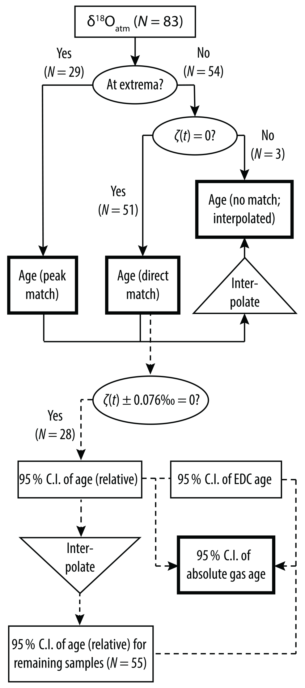
Figure 3Schematic workflow of timescale synchronization by δ18Oatm (solid lines) and uncertainty estimates (dashed lines). Rectangles refer to data, circles include conditional statements, and triangles stand for mathematical operations. Arrows mark the workflow. Boxes in bold lines indicate that we have arrived at the final answer. Definition of ζ(t) is given by Eq. (4) in the text. C.I.: confidence interval.
In the first step, an extreme is defined when the δ18Oatm sample is higher (“peak”) or lower (“trough”) than the two adjacent δ18Oatm samples. The advantage of this approach is that it relies on the prominent features within the δ18Oatm records and is not very sensitive to the systematic offset (if any) between the records. Out of 83 δ18Oatm samples from S27, 29 (35 %) were identified as peaks/troughs and matched to corresponding features in the EDC δ18Oatm record.
However, not all points are at peaks or troughs. To maximally utilize the rest of the data, we proceed with step (2) and constructed ζ, a function of time t, defined below:
Note that δ18Oatm(t),EDC here is linearly interpolated between individual δ18Oatm points reported in Extier et al. (2018). We seek the age t that satisfies in which case a “direct match” is deemed successful and a corresponding EDC age is assigned to the S27 sample. In total, 51 samples (61 %) have their ages assigned this way.
Finally, if a δ18Oatm(t),S27 point is neither at a peak or trough nor successfully matched to EDC δ18Oatm, the age of this data point is constrained by the ages of its adjacent δ18Oatm points, as in step (3). Only three points (4 %) fall into the final category. The age assignment method and result of each S27 δ18O datum are listed in Supplement Table S3, along with their uncertainties. The final reported uncertainties associated with the gas chronology consist of three parts: the analytical uncertainties of δ18Oatm, the relative uncertainties of S27 chronology to EDC chronology, and the inherent uncertainties of the EDC chronology itself. Readers are referred to the Supplement for a more detailed discussion.
2.5 Firn densification inverse modeling
Firn densification models typically use accumulation rate and mean annual surface temperature to calculate Δage (see Lundin et al., 2017, for a more in-depth review). In our case, however, we seek to do the opposite, using the temperatures inferred from the isotopic composition of the ice δDice, and the Δage to estimate accumulation rates for S27. Δage is calculated by subtracting the gas age (obtained according to Sect. 2.4) from the ice age (from Spaulding et al., 2013) of the same depth.
Here, we employ an empirical firn densification model from Herron and Langway (1980), abbreviated as H-L hereafter. H-L has the merits of transparency and simplicity, as only three properties are involved. In any case, densification models are trained against similar data and simulate similar relations between temperature, accumulation rate, close-off depth, and close-off age (Δage). A limitation of empirical firn densification models is that their range of calibration may not include low-accumulation sites. To evaluate the performance of the H-L model, we compare the model output with the present-day accumulation rate in the vicinity of S27 from Dadic et al. (2015).
The H-L model divides firn densification into two stages. In the first stage (firn density <550 kg m−3), the densification process is independent of accumulation rate and is a function of surface temperature. At the threshold density of 550 kg m−3, the elapsed time since snow deposition on the surface, t0.55, is given by
k0 is a temperature-dependent rate constant [], in which T equals temperature, in Kelvin (to be inferred from δDice), A is the accumulation rate (m yr−1), ρi is the density of ice (917 kg m−3), and ρ0 is the density of surface snow, which we assume to be 360 kg m−3 (Herron and Langway, 1980). In the second stage, t, the total elapsed time since snow deposition, is calculated from firn density (ρ) using the following relationship:
where k1 is another temperature-dependent rate constant [], and ρ is the firn density at this depth (Herron and Langway, 1980). A key step in the firn densification process is bubble close-off, at which point gases can no longer diffuse within the firn and become “locked” between ice grains. For S27, bubble close-off is assumed to occur when the firn density reaches 830 kg m−3. At this density, t in Eq. (6) equals Δage.
An additional parameter needed to solve accumulation rate A from Eqs. (5) and (6) is the site temperature, T. In order to derive historic Site 27 temperatures, we use δDice reported in Spaulding et al. (2013) and a regional isotope–temperature sensitivity of 4.0 established at the nearby Taylor Dome (Steig et al., 2000). We acknowledge that this isotope–temperature relationship could change over time, but it is not well-constrained in southern Victoria Land (Steig et al., 2000). A recent estimate of isotope–temperature sensitivity for Talos Dome located in northern Victoria Land yields a slope of 7.0 (Buizert et al., 2021). Increasing the isotope–temperature sensitivity by 75 % to 7.0 reduces the accumulation rate estimates by no more than 20 %. The main conclusions of this paper would remain unchanged.
Modern-day Allan Hills δDice of −270 ‰ (Dadic et al., 2015) and mean annual temperature of −30 ∘C (Delisle and Sievers, 1991) are used to calculate past temperatures. We note that the Allan Hills surface snow δDice value found by Dadic et al. (2015) is −257 ‰, but we opted not to use this value for the following reasons. First, this δDice value is ∼30 ‰ heavier than the Last Interglacial δDice observed in the S27 core (Fig. 2), implying an unlikely 7.5 ∘C warming today compared to the LIG. Second, the deuterium excess value of the same surface snow is negative (−5 ‰), which may have been the result of post-depositional processes (Dadic et al., 2015). Third, a gradient of δDice and deuterium excess along depth is observed, reaching −270 ‰ and 1 ‰ at the depth of ∼0.25 m, respectively. Below this depth, both δDice and deuterium excess show little variability (Fig. 2 in Dadic et al., 2015). We interpret these observations to indicate post-depositional alterations to the isotopic compositions of snow above 0.25 m and therefore use the δDice values below 0.25 m (−270 ‰) for the isotope–temperature calibration. In any case, using the nominal surface δDice value of −257 ‰ for calibration increases the accumulation rate estimates by less than 10 %.
Finally, we ran a Monte Carlo simulation for each single Δage datum with 100 000 iterations to derive the distribution of accumulation rate estimates given the Δage uncertainties (see the Supplement for its derivations). The reported accumulation rate comes from the value with the highest number of occurrences (the mode), and its 95 % confidence interval is bracketed by the values at the 2.5th and 97.5th percentile, respectively (Fig. S5 in the Supplement).
The H-L model also produces estimates of the depth at which firn density crosses the bubble close-off threshold. The interval from the close-off depth to the surface contains three components: the lock-in zone where ice layers are impenetrable and vertical transport is inhibited (hLIZ); the height of the diffusive column where the gravitational separation of heavy isotopes occurs (hdiff); and the height of the convective zone where vigorous mixing by convective air motions prevents the establishment of gravitational profiles (hconv; Severinghaus et al., 2010).
The following barometric equation is used to link the diffusive column height hdiff to the δ15N enrichment (Sowers et al., 1989):
where Δm is the difference between the molecular weight of 15N14N and 14N14N (0.001 kg mol−1), g is the gravitational acceleration constant (9.8 m s−2), R is the ideal gas constant (8.314 ), and T is the temperature (in Kelvin). hdiff is calculated by subtracting the hLIZ (3 m) and hconv (0 m) from the bubble close-off depth calculated using the H-L model.
3.1 A new gas chronology for S27
Figure 4 shows the result of synchronization between the S27 and EDC via δ18Oatm. Each of the δ18Oatm minima and maxima associated with orbital-scale insolation variations between 105 and 245 ka is successfully identified in S27, including the δ18Oatm peak around 180 ka that was previously missing in Spaulding et al. (2013). Overall, the strong similarities between the two δ18Oatm series give confidence to the stratigraphic integrity of the S27 gas record. The match between the S27 and EDC δ18Oatm is particularly tight between 105 and 145 ka, which corresponds to the depth interval of 7 m to 145 m in S27. δ18Oatm samples older than 145 ka show more offsets between S27 and EDC. This is noticeably evidenced by the scattering of S27 δ18Oatm data around the EDC curve between 202 and 210 ka. One possible explanation for the increased scatter is a decline in core quality in S27, where ice below ∼145 m is heavily fractured and visibly characterized by uneven surface cracks. This explanation is supported by more variable S27 values below 150 m (Fig. S3), suggesting a critical point between 145 and 150 m, below which depth data reproducibility deteriorates substantially. This variability would be accompanied by more noise in the δ18Oatm record despite the corrections for gas loss in the deeper part of the ice core.
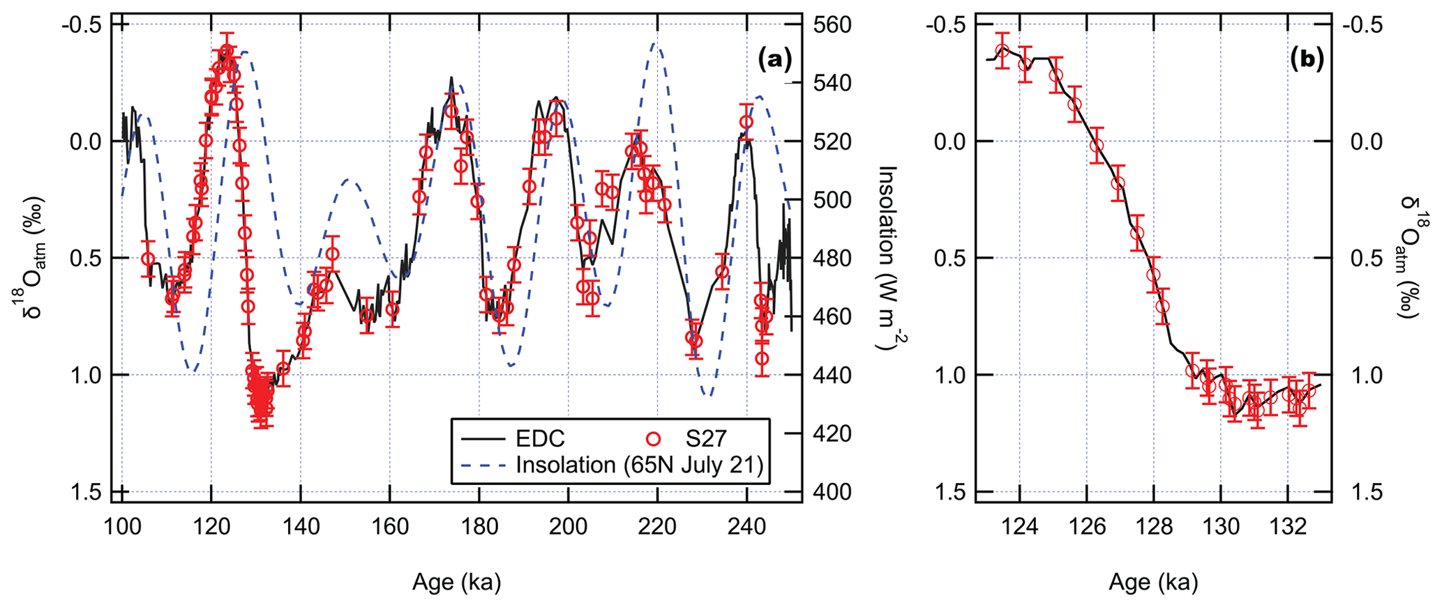
Figure 4δ18Oatm measured in S27 (red) was matched to a high-resolution δ18Oatm record from EDC (black) between 100 and 250 ka by Extier et al. (2018): (a) the whole record between 114 and 255 ka, accompanied by the Northern Hemisphere (65∘ N) 21 July insolation curve (dashed blue), and (b) a close-up view between 123 and 133 ka. S27 δ18Oatm data include those reported in Spaulding et al. (2013) and additional δ18Oatm samples measured in this work. Error bars represent 95 % confidence interval of the combined EDC and S27 δ18Oatm measurements, following the approaches described in the Supplement.
CH4 (N=12) and CO2 (N=17) samples measured at S27 are plotted on the δ18Oatm-derived timescale in Fig. 5. Also shown for comparison are an EDC CH4 (Loulergue et al., 2008) record and a composite high-resolution CO2 record built upon multiple Antarctic ice cores (Bereiter et al., 2015, and references therein). Because the relative uncertainties associated with greenhouse gas measurements are smaller than the errors of the δ18Oatm analyses, greenhouse gases are used to further improve the δ18Oatm-derived gas chronology. Below we describe the process of fine-tuning the δ18Oatm-derived gas chronology to better match greenhouse gas measurements in the reference records. We also tabulate chosen tie points between the S27 and EDC CH4, as well as S27 and the composite CO2, in Supplement Table S2. The timescale adjustment below only applies to the interval between 115.7 and 147.2 ka: at 115.7 ka, both S27 CO2 and CH4 agree well with the coeval values observed in the reference records, and S27 and EDC δ18Oatm values were both extrema at 147.2 ka. They are selected as “anchor points” that do not involve any adjustment.
The most prominent feature in Fig. 5 is the greenhouse gas peak at ∼128 ka. There is a 2 ppm offset in this CO2 peak observed in the S27 record compared to the composite record (within the analytical uncertainty). There is an offset of only 163 years between the ages of the CO2 peaks recorded at S27 and in the composite record. We therefore tied the CO2 peak at 128.6 ka in S27 to the peak at 128.5 ka in reference time series. In the ice below, both CH4 and CO2 in S27 show a clear increasing trend with time going upward towards the maximum, corresponding to the deglacial rise of greenhouse gases. We tied the S27 CH4 data point at 144.2 ka with the EDC CH4 point at 144.8 ka. We acknowledge that the low sampling resolution of greenhouse gases below 140 m precludes more rigorous evaluation of the δ18Oatm-derived gas chronology.
Ages of the data points in between the anchor and tie points were re-sampled by linear interpolation. Uncertainties of the gas chronology are assumed to be unaffected by this fine-tuning. The new, complete gas chronology for S27 is presented in Supplement Table S3. We emphasize that the effect of this fine-tuning on the gas chronology is at most 600 years (at 144.2 ka), and in many cases much smaller. Even with the timescale solely derived from δ18Oatm, the conclusions of this study remain the same. The final uncertainty associated with the new S27 gas age scale (1σ) varies between ±1600 and ±4000 years, averaging ±2200 years, also listed in Supplement Table S3.
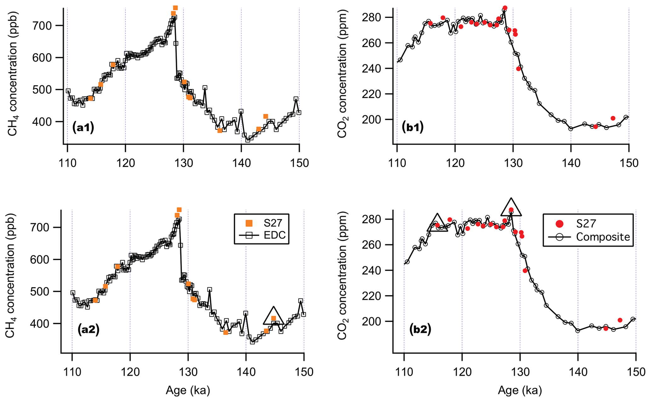
Figure 5CH4 and CO2 measured in S27 plotted on the timescale developed solely on δ18Oatm (a1, b1) and on the chronology after greenhouse gas synchronization (a2, b2). Tie points and anchor points are marked in triangles. EDC CH4 data are from Loulergue et al. (2008), composite CO2 data from multiple ice cores are from Bereiter et al. (2015) and references therein, and the timescale (AICC2012) is from Veres et al. (2013) and Bazin et al. (2013).
3.2 Ice-age–gas-age difference (Δage)
Below we evaluate Δage calculated by subtracting gas age from ice age. Gas age comes from the δ18Oatm-derived, CH4- and CO2-adjusted gas chronology from this work. Ice age comes from the δDice-based ice chronology established in Spaulding et al. (2013). All chronologies discussed here have been converted to AICC2012, the most up-to-date Antarctic ice core timescale (Veres et al., 2013; Bazin et al., 2013).
The relationship between the depth and the ice and gas age in S27 is shown in Fig. 6. The ice age is younger than the gas age between 192 and 204 m. This result is glaciologically impossible given the presence of a diffusive column and the measured positive δ15N values (Fig. S6 in the Supplement). Such discrepancies could arise from the ambiguous matching of δDice, severe impact of gas losses on δ18Oatm, or both.
The interval between 115 and 140 ka in S27 is where the gas and ice age scales are both well-constrained, corresponding to a depth range of 10.05 and 134.55 m. The selection of δ18Oatm samples from this section was done so that there are no visible fractures and cracks, and we therefore limit our subsequent discussion of Δage to the interval between 115 and 140 ka. Here, δDice values represent deglacial warming, and the cooling after the LIG, allowing unambiguous feature matching (e.g., the distinct LIG peak around 128.2 ka). We acknowledge that different ice core water isotope records may not be perfectly synchronous, and it is possible that the selected tie points do not capture the true peaks (or troughs) due to the discrete sampling of the ice cores. These errors are incorporated in the form of relative uncertainty in the ice age scale and propagated along with the intrinsic uncertainty associated with EDC Δage on the AICC2012 timescale into the S27 Δage uncertainty. We discuss those considerations in greater detail in the Supplement.
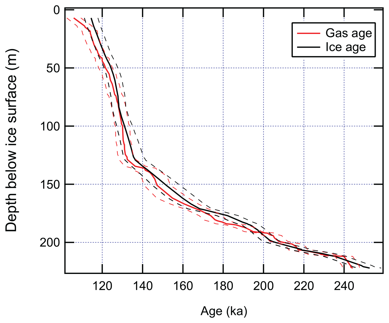
Figure 6Depth profile of gas age (red) and ice age (black) in S27. Dashed lines represent the 95 % uncertainty of the absolute age.
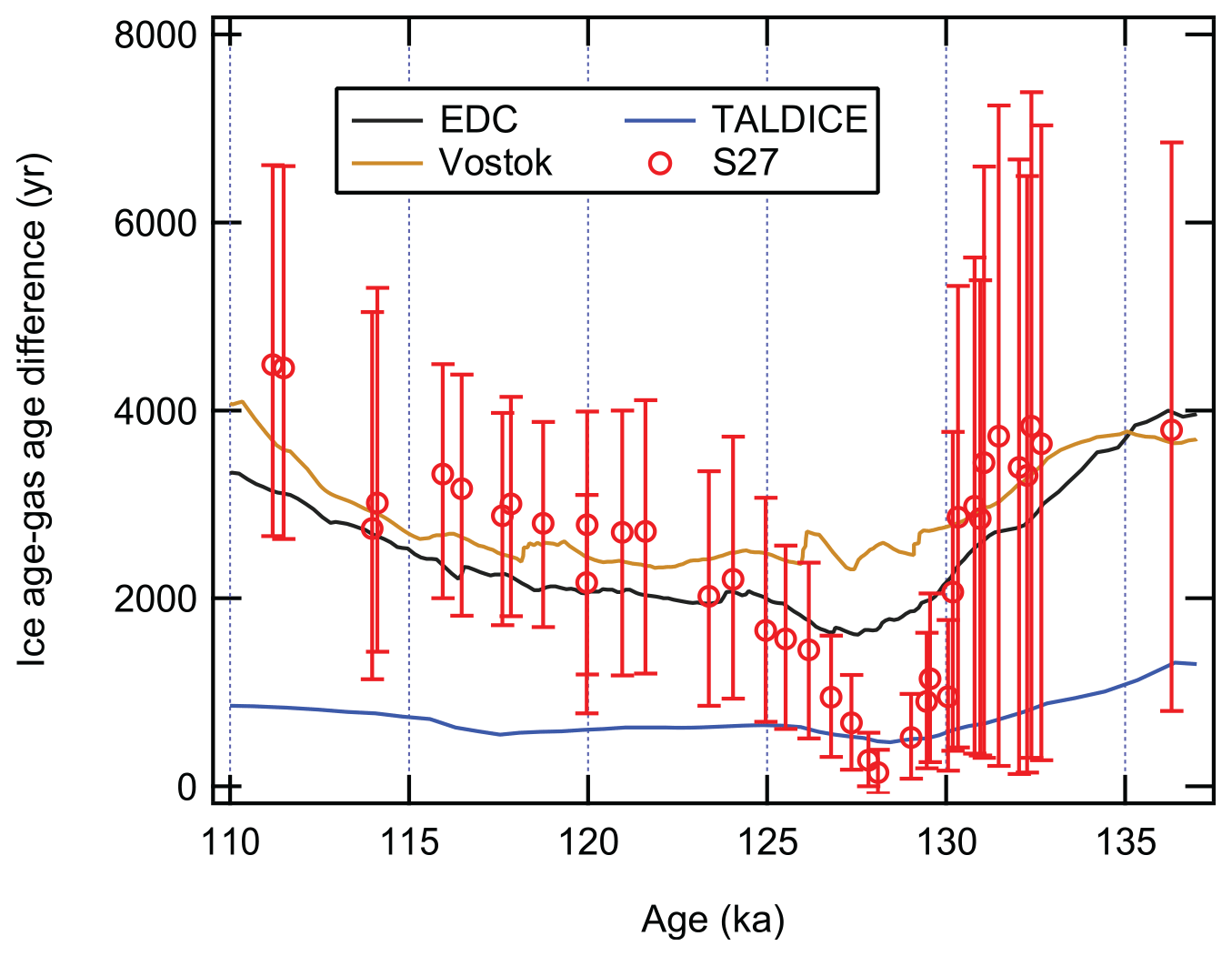
Figure 7Ice-age–gas-age difference (Δage) between 110 and 136 ka in S27 (red), Talos Dome (TALDICE; blue), Vostok (brown), and EDC (black). This age interval corresponds to the depth range of 10.05 to 134.55 m in S27, where the measured samples are free from any visible fractures. TALDICE, Vostok, and EDC Δage data are from Bazin et al. (2013) and references therein. All four Δage records show a similar pattern during Termination II, with minimum values reached around ∼128 ka. Error bars in S27 data represent the 95 % confidence interval of the Δage estimates. Note that the Δage values are plotted on the gas age scale and the confidence intervals of the S27 Δage points are asymmetrical.
Δage of S27 between 115 and 140 ka is plotted along with the Δage estimates in Talos Dome, EDC, and Vostok (Fig. 7). Apart from the similarities in the shape of the Δage curve across Termination II between the four records, a prominent feature here is the very low Δage of S27 during the LIG, reaching its minimum value of 145 years (95 % C.I.: 27–300 years) at 128.2 ka. In the entire record, small Δage values are not limited to 128 ka. For example, the Δage reaches less than 500 years at ∼142 ka, but we caution that the interval between 140 and 145 ka is under-constrained. Between the interval of 140 and 145 ka, there are only two ice age tie points (Fig. 2) and four δ18Oatm measurements (Fig. 4). The very small Δage around 142 ka cannot be established as a robust feature. By contrast, there are 15 δ18Oatm samples in the 5000-year interval from 128 to 133 ka and four ice age tie points within the interval between 125 and 130 ka.
Finally, we acknowledge that given the noisy nature of the S27 δDice records (Figs. 2 and S7 in the Supplement), it is possible that the Δage – and by inference the ice accumulation rates – could have larger errors than reported here, which we discuss in greater detail in the Supplement. A more refined ice chronology, perhaps made available by absolute-dating tephra layers and synchronizing ion content such as sulfate, will greatly improve the ice chronology of S27. However, the Allan Hills volcanological records are dominated by regional tephra, with similar composition and contamination by plagioclase crystals from the basement bedrock. In any case, past efforts to date tephra layers directly using the Ar method were not successful (William McIntosh, personal communications, 2010). Abundant regional volcanic signals further complicate direct correlation of the Allan Hills volcanic record with deep Antarctic ice cores (Nishio et al., 1985).
3.3 Accumulation rates
Figure 8 shows the estimated accumulation rate in S27 versus time between 115 and 140 ka, determined from estimates of Δage (i.e., solving A from t in Eq. 6). Accumulation rates in three other aforementioned Antarctic ice cores (Talos Dome, EDC, and Vostok) during the same time interval are shown for comparison. While the accumulation rate at other sites began to increase around 136 ka, coinciding with the onset of Termination II, the accumulation rate at S27 remained low for another ∼3000 years, averaging 0.0026 m yr−1 from 140.1 to 133.2 ka.
Beginning at 132.2 ka, S27 accumulation rate increased by an order of magnitude within 4000 years and reached its maximum value at 0.086 m yr−1 (95 % C.I.: 0.059–0.904 m yr−1) at 128.2 ka. The peak in S27 accumulation rates coincides with ∼128 ka peak warming in Antarctica, as well as with the maximum accumulation rate recorded in three other East Antarctic ice cores. We acknowledge the large uncertainty here, as high accumulation rate estimates are associated with a very small Δage values and hence large relative errors. That said, this particular small Δage is a robust estimate because the precise match between δDice peaks around ∼128 ka puts a firm constraint on ice age (Fig. 2), and the monotonic deglacial δ18Oatm change means small gas age uncertainty (Fig. 4b). In addition, this estimate agrees with the peak LIG accumulation rate at the nearby Taylor Dome deduced from 10Be activities in the ice (0.074 m yr−1; Steig et al., 2000). Importantly, even the most conservative accumulation rate estimate of 0.059 m yr−1 (the lower bound of the 95 % C.I.) still means an order-of-magnitude increase in the LIG S27 accumulation rate.
The elevated snow accumulation during the LIG at S27 was a transient phenomenon as by 125.5 ka, accumulation rates had already dropped below 0.075 m yr−1, the present-day accumulation rate observed in the vicinity of Allan Hills (Dadic et al., 2015), and further declined to a baseline value of less than 0.005 m yr−1 after 120 ka. The H-L model in general produce estimates for δ15N values that agree with the observations, except between 125 and 130 ka where the H-L model appears to overestimate δ15N (Fig. S6). This could be explained by the presence of a convective column (Severinghaus et al., 2010). We note, however, that the occurrence of deep convection in the firn column does not impact accumulation rate estimates from Δage because we are not relying on δ15N values to reconstruct lock-in depths.

Figure 8Accumulation rate between 115 and 140 ka in S27 (red), Talos Dome (TALDICE; blue), Vostok (brown), and EDC (black). Note that the y axis is plotted on logarithm scales. Accumulation rates of EDC, TALDICE, and Vostok are from Bazin et al. (2013) and the references therein. Error bars represent the 95 % confidence interval for S27 accumulation rate estimates. The dashed line in red represents the present-day accumulation rate (0.0075 m yr−1) in the vicinity of Allan Hills (Dadic et al., 2015).
Today, moisture transport into Allan Hills vicinity is primarily in the form of synoptic-scale low-pressure weather systems (Cohen et al., 2013) modulated by the position and intensity of the Amundsen Sea Low and the austral westerlies (Bertler et al., 2004; Patterson et al., 2005). In this context, one way to interpret the pronounced increase in S27 accumulation rates during Termination II is a transient reorganization of large-scale atmospheric circulation due to the poleward shift in the westerly wind belt associated with the deglacial warming. This mechanism is commonly invoked to explain the CO2 rise during ice age terminations (Toggweiler et al., 2006). Simulations also reveal increased precipitation in southern Victoria Land by the end of the 21st century due to enhanced moisture transport towards the interior of the continent in a warmer climate state (Krinner et al., 2007). Atmospheric CO2 during Termination II began to increase around 140 ka and peaked around 128.5 ka, coinciding with the accumulation rate peak in S27 (Fig. 9). The contraction of the westerlies would push the storm tracks further into the Antarctic continent. The results would be increased precipitation at otherwise low-accumulation sites and the peak in accumulation concomitant with the maximum atmospheric CO2.
In addition to large-scale circulation shifts, local to regional changes must also be at work for two reasons. First, the peak accumulation rate at S27 during the LIG is an order of magnitude larger than the average S27 accumulation rate between 140 and 133 ka. This difference is at least 3 times larger than the doubling or tripling in accumulation rates recorded in other Antarctic ice cores (Fig. 8). Second, the S27 accumulation rate started to increase at 132 ka and lagged the Antarctic warming and CO2 increase (Fig. 9). The abrupt change in accumulation rates could possibly be linked to the migration of local ice domes and the subsequent shifts in accumulation gradient, as revealed by some pioneering studies in this region (Morse et al., 1998, 1999). More recently, studies comparing the Taylor Dome and Taylor Glacier blue ice accumulation rates find a reversal in the accumulation gradient in the Last Glacial Maximum compared to Marine Isotope Stage 4 (MIS) without glacial–interglacial transitions (Baggenstos et al., 2018; Menking et al., 2019). We cannot fully rule out this possibility. However, we note that the peak LIG accumulation rate estimated from S27 is comparable to the Taylor Dome ice record (0.074 m yr−1; Steig et al., 2000) and Talos Dome (0.101 m yr−1; Bazin et al., 2013). It appears that the high accumulation rates observed in the LIG are a regional signal in Victoria Land. We thus proceed with the interpretation that the increase in accumulation rate during MIS 5e reflects a regional climatic shift. A more rigorous test would be to extend the accumulation history beyond 140 ka and to seek a large accumulation increase in glacial intervals.
We hypothesize that the peak S27 accumulation rate at 128 ka may reflect more open-ocean conditions in the Ross Sea. More open-water conditions near S27 could result from (1) reduced sea ice extent and an increase in polynya size, and/or (2) the retreat of the Ross Ice Shelf. Our first hypothesis concerning sea ice extent is supported by the blue ice record from the Mt Moulton BIA ( S, W; Fig. 1) near the Ross Sea coast in West Antarctica. The Mt Moulton record clearly documents an increase in sea salt concentrations and the lowest level of non-sea-salt sulfate during the peak LIG warming, interpreted as a minimum extent of sea ice and therefore the proximity of Mt Moulton ice field to an open ocean at 128 ka (Korotkikh et al., 2011). Moreover, Holloway et al. (2016) demonstrate that the retreat of winter sea ice in the Southern Ocean is fully capable of explaining the distinctive 128 ka δ18O isotope peak observed in Antarctic ice cores, although it should be noted that the inferred sea ice retreat in the Ross Sea is minimal in Holloway et al. (2016). If our hypothesis of more open-water conditions in the Ross Sea is correct, an LIG spike in sea salt concentration similar to that in the Mt Moulton ice record should also be visible in the S27 record. Furthermore, as moisture originating from a higher latitude generally has lower deuterium excess values, the open-water conditions at the peak of the LIG would lower the deuterium excess in the S27 ice. We note, however, that no aerosol or deuterium excess data from S27 are available at present.
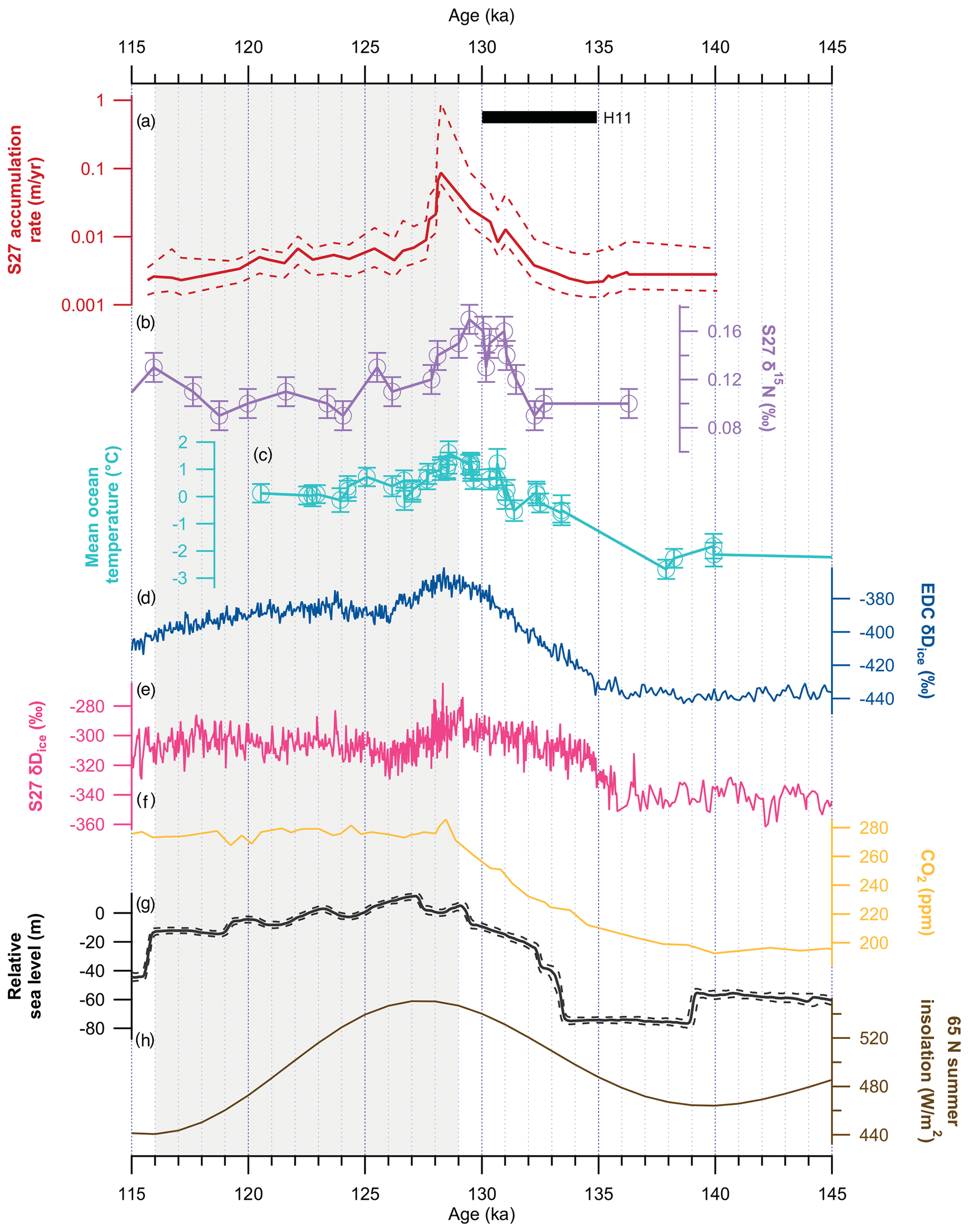
Figure 9Paleoclimate records during Termination II and the Last Interglacial. (a) S27 accumulation rate (this study) deduced from ice without any visible fractures. (b) δ15N of N2 in S27 (this study). (c) Mean ocean temperature based on noble gas ratios (Shackleton et al., 2020). (d) S27 stable water isotope records (Spaulding et al., 2013). (e) EPICA Dome C δDice records (Jouzel et al., 2007). (f) Atmospheric CO2 (Bereiter et al., 2015, and references therein). (g) Sea level relative to the present day inferred from δ18O of Red Sea planktonic foraminifera with 95 % confidence interval marked by the dashed lines (Rohling et al., 2019). (h) The 21 July insolation at 65∘ N. Shaded zone marks the LIG. The black bar marks Heinrich event 11 (H11).
The second hypothesis concerns the Ross Ice Shelf (RIS). Since the Last Glacial Maximum (LGM) the RIS has shrunk in size (Ship et al., 1999; Yokoyama et al., 2016), and recent work on glacial deposits in the southern Transantarctic Mountains reveals rapid grounding line retreat in the central and western Ross Sea in the early Holocene (Spector et al., 2017). Morse et al. (1998) first proposed that the elevated topography and the expansion of RIS during the LGM drove the storms heading towards Victoria Land northward, supported by later studies such as Aarons et al. (2016). If the RIS has been capable of exerting an influence on the synoptic weather systems over the last 13 000 years, the same underlying mechanism could also be operating in the LIG. That is, a further retreat of RIS led to the southward displacements of storm tracks and the enhancement of moisture transport into Site 27's accumulation region. Indeed, surface airflow into Victoria Land via the Ross Sea is enhanced in some numerical simulations where the WAIS and its adjacent ice shelves are removed (Steig et al., 2015). McKay et al. (2012) in addition suggest the absence of ice shelf cover in the western Ross Sea sometime in the past 250 000 years, a scenario compatible with the LIG retreat of RIS inferred from the S27 accumulation rate record. We acknowledge that the hypothesized response of atmospheric circulation to the absence of the RIS and reduced sea ice extent requires more examination by climate models.
The reduced ice shelf extent in the LIG has important implications for the stability of the West Antarctic Ice Sheet, as a widespread ice shelf retreat could signify the breakup of continental ice masses (DeConto and Pollard, 2016; Garbe et al., 2020). The inference of increased open-ocean water in the Ross Sea during the LIG aligns with other observations. Several lines of geologic evidence point to a rising sea level in the early LIG between 129 and 125 ka, implying substantial mass losses from continental ice sheets (e.g., McCulloch and Esat, 2000; O'Leary et al., 2013; Dutton et al., 2015b). Temperature reconstructions for north Greenland show similar-to-modern values at 129 ka (NEEM community members, 2013) and suggest that the Greenland Ice Sheet (GIS) was not responsible for the sea-level high stand at that time (Yau et al., 2016). In this case, the elevated sea level beginning ∼129 ka would have to significantly result from mass losses in West Antarctica, according to a recent LIG sea-level reconstruction with high temporal resolution and precise chronological controls (Fig. 9; Rohling et al., 2019). This reconstruction is further reinforced by basin-wide ice losses in the Weddell Sea as early as 129 ka deduced from a blue ice record from Patriot Hills, West Antarctica ( S, W; Fig. 1; Turney et al., 2020).
An open Ross Sea at 128 ka inferred from the S27 ice record presented in this work supports the proposed early collapse of the WAIS in the LIG and underscores the vulnerability of Antarctic ice shelves and ice sheets to rising ocean temperatures during Termination II, possibly linked to Heinrich event 11 between 135 and 130 ka (Fig. 9; Marino et al., 2015). For example, a chain of events could be that meltwater discharge in the North Atlantic weakened the Atlantic Meridional Overturning Circulation and consequently reduced the northward cross-equatorial heat transport, resulting in Southern Hemisphere warming, southward shifts of the intensified westerlies, and enhanced CO2 ventilation in the Southern Ocean (Menviel et al., 2018). Even if the S27 accumulation rate increase since 132 ka was not accompanied by the collapse of the WAIS in the early LIG, our results appear at odds with some model predictions that the collapse of the WAIS only began at 127 ka while the RIS remained largely intact (e.g., Clark et al., 2020). Based on the accumulation rate history, the Ross Ice Shelf appeared to quickly readvance soon after the conclusion of peak warming. By 125 ka the open oceans conducive to a high accumulation rate in S27's accumulation region became reverted to its previous conditions covered by ice. Since it is unlikely that the WAIS could recover within 3000 years, this recovery likely stems from the fact that the Ross Ice Shelf is partly fed by the East Antarctic Ice Sheet (Rignot et al., 2011), which remained stable during the LIG.
Finally, regardless of the cause(s) of the LIG spike in the S27 accumulation rate, it has significant glaciological implications in terms of ice flow modeling for the Allan Hills BIA, where ice older than 2 Ma (where Ma indicates millions of years before present) has been discovered in sites disconnected from the main ice flow line (Yan et al., 2019). Recent ice-penetrating radar surveys and ice flow modeling by Kehrl et al. (2018) have suggested the potential preservation of a stratigraphically continuous ice record, with 1 Ma ice located 25 to 35 m above the bedrock. The modeling efforts by Kehrl et al. (2018) assume no-higher-than-present accumulation rates in the past and constant sublimation rates that control the exhumation of ice along the flow line. In light of the discovery of this work, models with the time-dependent accumulation rate constrained by observations could better predict the age–depth profile. Nonetheless, S27 itself provides a continuous, readily available ice record for Termination II and the LIG with a nominal resolution of 285.7 yr m−1 in the upper 145 m with good ice core quality, making the Allan Hills BIA an appealing archive for paleoclimate investigations targeting the LIG.
We present an improved gas chronology for a shallow blue ice record (S27) drilled in the Allan Hills Blue Ice Area, East Antarctica, located in close proximity to the current northwest margin of the Ross Ice Shelf (RIS). The new S27 gas chronology is derived from the δ18O of O2 trapped in the ice. Complementary CH4 and CO2 measurements validate and refine the gas chronology, paving the way for future utilization of S27 samples. The calculation of accumulation rate on the basis of the ice-age–gas-age differences between 115 and 140 ka in S27 reveals a dramatic increase in accumulation rate since 132 ka peaking at 128.2 ka and coinciding with the peak LIG Antarctic warming and atmospheric CO2.
We hypothesize that in addition to changes in the large-scale atmospheric circulation affecting precipitation on the Antarctic continent, sea ice and ice shelf extent could alter local meteorological boundary conditions and lead to the observed spike in accumulation rate. A greater reduction in size of the RIS would cause the storm tracks that bring substantial precipitation to Victoria Land today to migrate farther south. The ice shelf retreat would also be compatible with a high sea-level stand around 129 ka sourced from the collapse of the West Antarctica Ice Sheet near the onset of the Last Interglacial period (Yau et al., 2016; Rohling et al., 2019). If this was the case, an early collapse of the WAIS (along with the RIS) in the LIG would underscore its vulnerability to rising temperatures.
Our data suggest that, soon after the conclusion of peak warming, the open ocean conducive to a high accumulation rate near S27's accumulation region once again became covered by ice by 125 ka. The depositional site of S27 returned to its previous conditions characterized by low accumulation rates similar to those today. We conclude that if the Ross Ice Shelf indeed collapsed early in the LIG, it would have quickly re-advanced by 125 ka, possibly fed by the ice streams sourced from the East Antarctic Ice Sheet.
In addition, S27 ice core data underlying this study will be made publicly available at the United States Antarctic Program Data Center upon the acceptance of this paper for publication with the following digital object identifiers (DOIs): https://doi.org/10.7265/N5NP22DF (S27 stable water isotope records) (Kurbatov et al., 2013); https://doi.org/10.15784/601424 (S27 gas isotopes) (Yan et al., 2021); and https://doi.org/10.15784/601425 (S27 greenhouse gas concentrations) (Yan and Brook, 2021).
The supplement related to this article is available online at: https://doi.org/10.5194/cp-17-1841-2021-supplement.
YY conceived the study conceptually. YY, MLB, EJB, AVK, and PAM designed the experiments. YY performed the new δ18Oatm analyses. JAH undertook earlier δ18Oatm measurements. NES measured δDice and established the ice chronology. YY carried out age synchronization and firn densification modeling. YY wrote the paper with inputs from all authors.
The authors declare that they have no conflict of interest.
Publisher's note: Copernicus Publications remains neutral with regard to jurisdictional claims in published maps and institutional affiliations.
We thank Michael Kalk, Jon Edwards, James E. Lee, Laura M. Chimiak, and Douglas S. Introne for their laboratory assistance. Discussion with James A. Menking on firn densification modeling improved the paper.
This research has been supported by the National Science Foundation, Directorate for Geosciences (grant nos. ANT-1443263, ANT-1443276, and ANT-1443306) and a Pan Family Postdoctoral Fellowship at Rice University to Yuzhen Yan.
This paper was edited by Eric Wolff and reviewed by Frédéric Parrenin and two anonymous referees.
Aarons, S. M., Aciego, S. M., Gabrielli, P., Delmonte, B., Koornneef, J. M., Wegner, A., and Blakowski, M. A.: The impact of glacier retreat from the Ross Sea on local climate: Characterization of mineral dust in the Taylor Dome ice core, East Antarctica, Earth Planet. Sc. Lett., 444, 34–44, https://doi.org/10.1016/j.epsl.2016.03.035, 2016.
Ahn, J., Brook, E. J., and Howell, K.: A high-precision method for measurement of paleoatmospheric CO2 in small polar ice samples, J. Glaciol., 55, 499–506, https://doi.org/10.3189/002214309788816731, 2009.
Baggenstos, D., Severinghaus, J. P., Mulvaney, R., McConnell, J. R., Sigl, M., Maselli, O., Petit, J. R., Grente, B., and Steig, E. J.: A horizontal ice core from Taylor Glacier, its implications for Antarctic climate history, and an improved Taylor Dome ice core time scale, Paleoceanogr. Paleoclimatol., 33, 778–794, https://doi.org/10.1029/2017PA003297, 2018.
Bazin, L., Landais, A., Lemieux-Dudon, B., Toyé Mahamadou Kele, H., Veres, D., Parrenin, F., Martinerie, P., Ritz, C., Capron, E., Lipenkov, V., Loutre, M.-F., Raynaud, D., Vinther, B., Svensson, A., Rasmussen, S. O., Severi, M., Blunier, T., Leuenberger, M., Fischer, H., Masson-Delmotte, V., Chappellaz, J., and Wolff, E.: An optimized multi-proxy, multi-site Antarctic ice and gas orbital chronology (AICC2012): 120–800 ka, Clim. Past, 9, 1715–1731, https://doi.org/10.5194/cp-9-1715-2013, 2013.
Bereiter, B., Eggleston, S., Schmitt, J., Nehrbass-Ahles, C., Stocker, T. F., Fischer, H., Kipfstuhl, S., and Chappellaz, J.: Revision of the EPICA Dome C CO2 record from 800 to 600 kyr before present, Geophys. Res. Lett., 42, 542–549, https://doi.org/10.1002/2014GL061957, 2015.
Bertler, N. A., Barrett, P. J., Mayewski, P. A., Fogt, R. L., Kreutz, K. J., and Shulmeister, J.: El Niño suppresses Antarctic warming, Geophys. Res. Lett., 31, L15207, https://doi.org/10.1029/2004GL020749, 2004.
Bindschadler, R., Choi, H., Wichlacz, A., Bingham, R., Bohlander, J., Brunt, K., Corr, H., Drews, R., Fricker, H., Hall, M., Hindmarsh, R., Kohler, J., Padman, L., Rack, W., Rotschky, G., Urbini, S., Vornberger, P., and Young, N.: Getting around Antarctica: new high-resolution mappings of the grounded and freely-floating boundaries of the Antarctic ice sheet created for the International Polar Year, The Cryosphere, 5, 569–588, https://doi.org/10.5194/tc-5-569-2011, 2011.
Buizert, C., Fudge, T. J., Roberts, W. H., Steig, E. J., Sherriff-Tadano, S., Ritz, C., Lefebvre, E., Edwards, J., Kawamura, K., Oyabu, I., and Motoyama, H.: Antarctic surface temperature and elevation during the Last Glacial Maximum, Science, 372, 1097–1101, https://doi.org/10.1126/science.372.6546.1051-f, 2021.
Clark, P. U., He, F., Golledge, N. R., Mitrovica, J. X., Dutton, A., Hoffman, J. S., and Dendy, S.: Oceanic forcing of penultimate deglacial and last interglacial sea-level rise, Nature, 577, 660–664, https://doi.org/10.1038/s41586-020-1931-7, 2020.
Cohen, L., Dean, S., and Renwick, J.: Synoptic weather types for the Ross Sea region, Antarctica, J. Climate, 26, 636–649, https://doi.org/10.1175/JCLI-D-11-00690.1, 2013.
Craig, H., Horibe, Y., and Sowers, T.: Gravitational separation of gases and isotopes in polar ice caps, Science, 242, 1675–1678, https://doi.org/10.1126/science.242.4886.1675, 1988.
Dadic, R., Schneebeli, M., Bertler, N. A., Schwikowski, M., and Matzl, M.: Extreme snow metamorphism in the Allan Hills, Antarctica, as an analogue for glacial conditions with implications for stable isotope composition, J. Glaciol., 61, 1171–1182, https://doi.org/10.3189/2015JoG15J027, 2015.
DeConto, R. M. and Pollard, D.: Contribution of Antarctica to past and future sea-level rise, Nature, 531, 591–597, https://doi.org/10.1038/nature17145, 2016.
Delisle, G. and Sievers, J.: Sub-ice topography and meteorite finds near the Allan Hills and the Near Western ice field, Victoria Land, Antarctica, J. Geophys. Res.-Planet., 96, 15577–15587, https://doi.org/10.1029/91JE01117, 1991.
Dreyfus, G. B., Parrenin, F., Lemieux-Dudon, B., Durand, G., Masson-Delmotte, V., Jouzel, J., Barnola, J.-M., Panno, L., Spahni, R., Tisserand, A., Siegenthaler, U., and Leuenberger, M.: Anomalous flow below 2700 m in the EPICA Dome C ice core detected using δ18O of atmospheric oxygen measurements, Clim. Past, 3, 341–353, https://doi.org/10.5194/cp-3-341-2007, 2007.
Dutton, A., Carlson, A. E., Long, A., Milne, G. A., Clark, P. U., DeConto, R., Horton, B. P., Rahmstorf, S., and Raymo, M. E.: Sea-level rise due to polar ice-sheet mass loss during past warm periods, Science, 349, aaa4019, https://doi.org/10.1126/science.aaa4019, 2015a.
Dutton, A., Webster, J. M., Zwartz, D., Lambeck, K., and Wohlfarth, B.: Tropical tales of polar ice: evidence of Last Interglacial polar ice sheet retreat recorded by fossil reefs of the granitic Seychelles islands, Quaternary Sci. Rev., 107, 182–196, https://doi.org/10.1016/j.quascirev.2014.10.025, 2015b.
Emerson, S., Quay, P. D., Stump, C., Wilbur, D., and Schudlich, R.: Chemical tracers of productivity and respiration in the subtropical Pacific Ocean, J. Geophys. Res.-Oceans, 100, 15873–15887, https://doi.org/10.1029/95JC01333, 1995.
Extier, T., Landais, A., Bréant, C., Prié, F., Bazin, L., Dreyfus, G., Roche, D. M., and Leuenberger, M.: On the use of δ18Oatm for ice core dating, Quaternary Sci. Rev., 185, 244–257, https://doi.org/10.1016/j.quascirev.2018.02.008, 2018.
Garbe, J., Albrecht, T., Levermann, A., Donges, J. F., and Winkelmann, R.: The hysteresis of the Antarctic ice sheet, Nature, 585, 538–544, https://doi.org/10.1038/s41586-020-2727-5, 2020.
Herron, M. M. and Langway, C. C.: Firn densification: an empirical model, J. Glaciol., 25, 373–385, https://doi.org/10.3189/S0022143000015239, 1980.
Holloway, M. D., Sime, L. C., Singarayer, J. S., Tindall, J. C., Bunch, P., and Valdes, P. J.: Antarctic last interglacial isotope peak in response to sea ice retreat not ice-sheet collapse, Nat. Commun., 7, 1–9, https://doi.org/10.1038/ncomms12293, 2016.
Hughes, T.: Is the West Antarctic ice sheet disintegrating? J. Geophys. Res., 78, 7884–7910, https://doi.org/10.1029/JC078i033p07884, 1973.
Jouzel, J., Masson-Delmotte, V., Cattani, O., Dreyfus, G., Falourd, S., Hoffmann, G., Minster, B., Nouet, J., Barnola, J. M., Chappellaz, J., and Fischer, H.: Orbital and millennial Antarctic climate variability over the past 800 000 years, Science, 317, 793–796, https://doi.org/10.1126/science.1141038, 2007.
Kehrl, L., Conway, H., Holschuh, N., Campbell, S., Kurbatov, A. V., and Spaulding, N. E.: Evaluating the duration and continuity of potential climate records from the Allan Hills Blue Ice Area, East Antarctica, Geophys. Res. Lett., 45, 4096–4104, https://doi.org/10.1029/2018GL077511, 2018.
Korotkikh, E. V., Mayewski, P. A., Handley, M. J., Sneed, S. B., Introne, D. S., Kurbatov, A. V., Dunbar, N. W., and McIntosh, W. C.: The last interglacial as represented in the glaciochemical record from Mount Moulton Blue Ice Area, West Antarctica, Quaternary Sci. Rev., 30, 1940–1947, https://doi.org/10.1016/j.quascirev.2011.04.020, 2011.
Krinner, G., Magand, O., Simmonds, I., Genthon, C., and Dufresne, J. L.: Simulated Antarctic precipitation and surface mass balance at the end of the twentieth and twenty-first centuries, Clim. Dyn., 28, 215–230, https://doi.org/10.1007/s00382-006-0177-x, 2007.
Kurbatov, A. V., Introne, D., Mayewski, P. A., and Spaulding, N.: Allan Hills Stable Water Isotopes, U.S. Antarctic Program (USAP) Data Center [data set], https://doi.org/10.7265/N5NP22DF, 2013.
Loulergue, L., Schilt, A., Spahni, R., Masson-Delmotte, V., Blunier, T., Lemieux, B., Barnola, J. M., Raynaud, D., Stocker, T. F., and Chappellaz, J.: Orbital and millennial-scale features of atmospheric CH4 over the past 800 000 years, Nature, 453, 383–386. https://doi.org/10.1038/nature06950, 2008.
Lundin, J. M., Stevens, C. M., Arthern, R., Buizert, C., Orsi, A., Ligtenberg, S. R., Simonsen, S. B., Cummings, E., Essery, R., Leahy, W., and Harris, P.: Firn Model Intercomparison Experiment (FirnMICE), J. Glaciol., 63, 401–422, https://doi.org/10.1017/jog.2016.114, 2017.
Marino, G., Rohling, E. J., Rodríguez-Sanz, L., Grant, K. M., Heslop, D., Roberts, A. P., Stanford, J. D., and Yu, J.: Bipolar seesaw control on last interglacial sea level, Nature, 522, 197–201, https://doi.org/10.1038/nature14499, 2015.
McCulloch, M. T. and Esat, T: The coral record of last interglacial sea levels and sea surface temperatures, Chem. Geol., 169, 107–129, https://doi.org/10.1016/S0009-2541(00)00260-6, 2000.
McKay, R., Naish, T., Powell, R., Barrett, P., Scherer, R., Talarico, F., Kyle, P., Monien, D., Kuhn, G., Jackolski, C., and Williams, T.: Pleistocene variability of Antarctic ice sheet extent in the Ross embayment, Quaternary Sci. Rev., 34, 93–112, https://doi.org/10.1016/j.quascirev.2011.12.012, 2012.
Menking, J. A., Brook, E. J., Shackleton, S. A., Severinghaus, J. P., Dyonisius, M. N., Petrenko, V., McConnell, J. R., Rhodes, R. H., Bauska, T. K., Baggenstos, D., Marcott, S., and Barker, S.: Spatial pattern of accumulation at Taylor Dome during Marine Isotope Stage 4: stratigraphic constraints from Taylor Glacier, Clim. Past, 15, 1537–1556, https://doi.org/10.5194/cp-15-1537-2019, 2019.
Menviel, L., Spence, P., Yu, J., Chamberlain, M. A., Matear, R. J., Meissner, K. J., and England, M. H.: Southern Hemisphere westerlies as a driver of the early deglacial atmospheric CO2 rise, Nat. Commun., 9, 2503, https://doi.org/10.1038/s41467-018-04876-4, 2018.
Mercer, J.: Antarctic Ice and Sangamon Sea Level, International Association of Scientific Hydrology Publication, 79, 217–225, 1968.
Mitchell, L., Brook, E., Lee, J. E., Buizert, C., and Sowers, T.: Constraints on the late Holocene anthropogenic contribution to the atmospheric methane budget, Science, 342, 964–966, https://doi.org/10.1126/science.1238920, 2013.
Morse, D. L., Waddington, E. D., and Steig, E. J.: Ice age storm trajectories inferred from radar stratigraphy at Taylor Dome, Antarctica, Geophys. Res. Lett., 25, 3383–3386, https://doi.org/10.1029/98GL52486, 1998.
Morse, D. L., Waddington, E. D., Marshall, H. P., Neumann, T. A., Steig, E. J., Dibb, J. E., Winebrenner, D. P., and Arthern, R. J.: Accumulation rate measurements at Taylor Dome, East Antarctica: Techniques and strategies for mass balance measurements in polar environments, Geogr. Ann. A, 81, 683–694, available at: https://onlinelibrary.wiley.com/doi/10.1111/1468-0459.00106 (last access: 14 September 2021), 1999.
NEEM community members: Eemian interglacial reconstructed from a Greenland folded ice core, Nature, 493, 489–494, https://doi.org/10.1038/nature11789, 2013.
Nishio, F., Katsushima, T., and Ohmae, H.: Volcanic ash layers in bare ice areas near the Yamato mountains, Dronning Maud Land and the Allan Hills, Victoria Land, Antarctica, Ann. Glaciol., 7, 34–41, https://doi.org/10.3189/S0260305500005875, 1985.
O'Leary, M. J., Hearty, P. J., Thompson, W. G., Raymo, M. E., Mitrovica, J. X., and Webster, J. M.: Ice sheet collapse following a prolonged period of stable sea level during the last interglacial, Nat. Geosci., 6, 796–800, https://doi.org/10.1038/ngeo1890, 2013.
Otto-Bliesner, B. L., Rosenbloom, N., Stone, E. J., McKay, N. P., Lunt, D. J., Brady, E. C., and Overpeck, J. T.: How warm was the last interglacial? New model–data comparisons, Philos. T. R. Soc. A, 371, 20130097, https://doi.org/10.1098/rsta.2013.0097, 2013.
Patterson, N. G., Bertler, N. A. N., Naish, T. R., and Morgenstern, U.: ENSO variability in the deuterium-excess record of a coastal Antarctic ice core from the McMurdo Dry Valleys, Victoria Land, Ann. Glaciol., 41, 140–146, https://doi.org/10.3189/172756405781813339, 2005.
Pritchard, H., Ligtenberg, S. R., Fricker, H. A., Vaughan, D. G., van den Broeke, M. R., and Padman, L.: Antarctic ice-sheet loss driven by basal melting of ice shelves, Nature, 484, 502–505, https://doi.org/10.1038/nature10968, 2012.
Rignot, E., Mouginot, J., and Scheuchl, B.: Ice flow of the Antarctic ice sheet, Science, 333, 1427–1430, https://doi.org/10.1126/science.1208336, 2011.
Rohling, E. J., Hibbert, F. D., Grant, K. M., Galaasen, E. V., Irvalı, N., Kleiven, H. F., Marino, G., Ninnemann, U., Roberts, A. P., Rosenthal, Y., and Schulz, H.: Asynchronous Antarctic and Greenland ice-volume contributions to the last interglacial sea-level highstand, Nat. Commun., 10, 5040, https://doi.org/10.1038/s41467-019-12874-3, 2019.
Severinghaus, J. P., Beaudette, R., Headly, M. A., Taylor, K., and Brook, E. J.: Oxygen-18 of O2 records the impact of abrupt climate change on the terrestrial biosphere, Science, 324, 1431–1434, https://doi.org/10.1126/science.1169473, 2009.
Severinghaus, J. P., Albert, M. R., Courville, Z. R., Fahnestock, M. A., Kawamura, K., Montzka, S. A., Mühle, J., Scambos, T. A., Shields, E., Shuman, C. A., and Suwa, M.: Deep air convection in the firn at a zero-accumulation site, central Antarctica, Earth Planet. Sc. Lett., 293, 359–367, https://doi.org/10.1016/j.epsl.2010.03.003, 2010.
Shackleton, S., Baggenstos, D., Menking, J. A., Dyonisius, M. N., Bereiter, B., Bauska, T. K., Rhodes, R. H., Brook, E. J., Petrenko, V. V., McConnell, J. R., and Kellerhals, T.: Global ocean heat content in the Last Interglacial, Nat. Geosci., 13, 77–81, https://doi.org/10.1038/s41561-019-0498-0, 2020.
Ship, S., Anderson, J., and Domack, E.: Late Pleistocene–Holocene retreat of the West Antarctic Ice-Sheet system in the Ross Sea: part 1 – Geophysical results, Geol. Soc. Am. Bull., 111, 1486–1516, https://doi.org/10.1130/0016-7606(1999)111%3C1486:LPHROT{%}3E2.3.CO;2, 1999.
Sowers, T., Bender, M., and Raynaud, D.: Elemental and isotopic composition of occluded O2 and N2 in polar ice, J. Geophys. Res.-Atmos., 94, 5137–5150, https://doi.org/10.1029/JD094iD04p05137, 1989.
Spaulding, N. E., Spikes, V. B., Hamilton, G. S., Mayewski, P. A., Dunbar, N. W., Harvey, R. P., Schutt, J., and Kurbatov, A. V.: Ice motion and mass balance at the Allan Hills blue-ice area, Antarctica, with implications for paleoclimate reconstructions, J. Glaciol., 58, 399–406, https://doi.org/10.3189/2012JoG11J176, 2012.
Spaulding, N. E., Higgins, J. A., Kurbatov, A. V., Bender, M. L., Arcone, S. A., Campbell, S., Dunbar, N. W., Chimiak, L. M., Introne, D. S., and Mayewski, P. A.: Climate archives from 90 to 250 ka in horizontal and vertical ice cores from the Allan Hills Blue Ice Area, Antarctica, Quaternary Res., 80, 562–574, https://doi.org/10.1016/j.yqres.2013.07.004, 2013.
Spector, P., Stone, J., Cowdery, S. G., Hall, B., Conway, H., and Bromley, G.: Rapid early-Holocene deglaciation in the Ross Sea, Antarctica, Geophys. Res. Lett., 44, 7817–7825, https://doi.org/10.1002/2017GL074216, 2017.
Steig, E. J., Morse, D. L., Waddington, E. D., Stuiver, M., Grootes, P. M., Mayewski, P. A., Twickler, M. S., and Whitlow, S. I.: Wisconsinan and Holocene climate history from an ice core at Taylor Dome, western Ross Embayment, Antarctica, Geogr. Ann. A, 82, 213–235, https://doi.org/10.1111/j.0435-3676.2000.00122.x, 2000.
Steig, E. J., Huybers, K., Singh, H. A., Steiger, N. J., Ding, Q., Frierson, D. M., Popp, T., and White, J. W.: Influence of West Antarctic ice sheet collapse on Antarctic surface climate, Geophys. Res. Lett., 42, 4862–4868, https://doi.org/10.1002/2015GL063861, 2015.
Suwa, M. and Bender, M. L.: Chronology of the Vostok ice core constrained by O2N2 ratios of occluded air, and its implication for the Vostok climate records, Quaternary Sci. Rev., 27, 1093–1106, https://doi.org/10.1016/j.quascirev.2008.02.017, 2008.
Toggweiler, J. R., Russell, J. L., and Carson, S. R.: Midlatitude westerlies, atmospheric CO2, and climate change during the ice ages, Paleoceanography, 21, PA2005, https://doi.org/10.1029/2005PA001154, 2006.
Turney, C. S., Fogwill, C. J., Golledge, N. R., McKay, N. P., van Sebille, E., Jones, R. T., Etheridge, D., Rubino, M., Thornton, D. P., Davies, S. M., and Ramsey, C. B.: Early Last Interglacial ocean warming drove substantial ice mass loss from Antarctica, P. Natl. Acad. Sci. USA, 117, 3996–4006, https://doi.org/10.1073/pnas.1902469117, 2020.
Veres, D., Bazin, L., Landais, A., Toyé Mahamadou Kele, H., Lemieux-Dudon, B., Parrenin, F., Martinerie, P., Blayo, E., Blunier, T., Capron, E., Chappellaz, J., Rasmussen, S. O., Severi, M., Svensson, A., Vinther, B., and Wolff, E. W.: The Antarctic ice core chronology (AICC2012): an optimized multi-parameter and multi-site dating approach for the last 120 thousand years, Clim. Past, 9, 1733–1748, https://doi.org/10.5194/cp-9-1733-2013, 2013.
Yan, Y. and Brook, E. J.: Greenhouse gas composition in the Allan Hills S27 ice core, U.S. Antarctic Program (USAP) Data Center [data set], https://doi.org/10.15784/601425, 2021.
Yan, Y., Bender, M. L., Brook, E. J., Clifford, H. M., Kemeny, P. C., Kurbatov, A. V., Mackay, S., Mayewski, P. A., Ng, J., Severinghaus, J. P., and Higgins, J. A.: Two-million-year-old snapshots of atmospheric gases from Antarctic ice, Nature, 574, 663–666, https://doi.org/10.1038/s41586-019-1692-3, 2019.
Yan, Y., Bender, M., and Higgins, J.: Stable isotope composition of the trapped air in the Allan Hills S27 ice core, U.S. Antarctic Program (USAP) Data Center [data set], https://doi.org/10.15784/601424, 2021.
Yau, A. M., Bender, M. L., Robinson, A., and Brook, E. J.: Reconstructing the last interglacial at Summit, Greenland: Insights from GISP2, P. Natl. Acad. Sci. USA, 113, 9710–9715, https://doi.org/10.1073/pnas.1524766113, 2016.
Yokoyama, Y., Anderson, J. B., Yamane, M., Simkins, L. M., Miyairi, Y., Yamazaki, T., Koizumi, M., Suga, H., Kusahara, K., Prothro, L., and Hasumi, H.: Widespread collapse of the Ross Ice Shelf during the late Holocene, P. Natl. Acad. Sci. USA, 113, 2354–2359, https://doi.org/10.1073/pnas.1516908113, 2016.