the Creative Commons Attribution 4.0 License.
the Creative Commons Attribution 4.0 License.
 | 13 Jul 2021
The unidentified eruption of 1809: a climatic cold case
Claudia Timmreck
Matthew Toohey
Davide Zanchettin
Stefan Brönnimann
Elin Lundstad
Rob Wilson
The “1809 eruption” is one of the most recent unidentified volcanic eruptions with a global climate impact. Even though the eruption ranks as the third largest since 1500 with a sulfur emission strength estimated to be 2 times that of the 1991 eruption of Pinatubo, not much is known of it from historic sources. Based on a compilation of instrumental and reconstructed temperature time series, we show here that tropical temperatures show a significant drop in response to the ∼ 1809 eruption that is similar to that produced by the Mt. Tambora eruption in 1815, while the response of Northern Hemisphere (NH) boreal summer temperature is spatially heterogeneous. We test the sensitivity of the climate response simulated by the MPI Earth system model to a range of volcanic forcing estimates constructed using estimated volcanic stratospheric sulfur injections (VSSIs) and uncertainties from ice-core records. Three of the forcing reconstructions represent a tropical eruption with an approximately symmetric hemispheric aerosol spread but different forcing magnitudes, while a fourth reflects a hemispherically asymmetric scenario without volcanic forcing in the NH extratropics. Observed and reconstructed post-volcanic surface NH summer temperature anomalies lie within the range of all the scenario simulations. Therefore, assuming the model climate sensitivity is correct, the VSSI estimate is accurate within the uncertainty bounds. Comparison of observed and simulated tropical temperature anomalies suggests that the most likely VSSI for the 1809 eruption would be somewhere between 12 and 19 Tg of sulfur. Model results show that NH large-scale climate modes are sensitive to both volcanic forcing strength and its spatial structure. While spatial correlations between the N-TREND NH temperature reconstruction and the model simulations are weak in terms of the ensemble-mean model results, individual model simulations show good correlation over North America and Europe, suggesting the spatial heterogeneity of the 1810 cooling could be due to internal climate variability.
- Article
(5025 KB) - Full-text XML
-
Supplement
(1943 KB) - BibTeX
- EndNote


The early 19th century (∼ 1800–1830 CE), at the tail end of the Little Ice Age, marks one of the coldest periods of the last millennium (e.g., Wilson et al., 2016; PAGES 2k Consortium, 2019) and is therefore of special interest in the study of inter-decadal climate variability (Jungclaus et al., 2017). It was influenced by strong natural forcing: a grand solar minimum (Dalton Minimum, ∼ 1790–1820 CE) and simultaneously a cluster of very strong tropical volcanic eruptions that includes the widely known Mt. Tambora eruption in 1815, an unidentified eruption estimated to have occurred in 1808 or 1809, and a series of eruptions in the 1820s and 1830s. Brönnimann et al. (2019a) point out that this sequence of volcanic eruptions influenced the last phase of the Little Ice Age by not only leading to global cooling but also by modifying the large-scale atmospheric circulation through a southward shift of low-pressure systems over the North Atlantic related to a weakening of the African monsoon and the Atlantic–European Hadley cell (Wegmann et al., 2014).
The Mt. Tambora eruption in April 1815 was the largest in the last 500 years and had substantial global climatic and societal effects (e.g., Oppenheimer, 2003; Brönnimann and Krämer, 2016; Raible et al., 2016). In contrast to the Mt. Tambora eruption, little is known about the 1809 eruption. Although there is no historical source reporting a strong volcanic eruption in 1809, its occurrence is indubitably brought to light by ice-core sulfur records, which clearly identify a peak in volcanic sulfur in 1809/1810 (Dai et al., 1991). Simultaneous signals in both Greenland and Antarctic ice cores with similar magnitude are consistent with a tropical origin, and analysis of sulfur isotopes in ice cores supports the hypothesis of a major volcanic eruption with stratospheric injection (Cole-Dai et al., 2009).
Based on ice-core sulfur records from Antarctica and Greenland, the 1809 eruption is estimated to have injected 19.3 ± 3.54 Tg of sulfur (S) into the stratosphere (Toohey and Sigl, 2017). This value is roughly 30 % less than the estimate for the 1815 Mt. Tambora eruption and roughly twice that of the 1991 Pinatubo eruption. Accordingly, the 1809 eruption produced the second-largest volcanic stratospheric sulfur injection (VSSI) of the 19th century and the sixth largest of the past 1000 years. For comparison, the Ice-core Volcanic Index 2 (IVI2) database (Gao et al., 2008) estimates that the 1809 eruption injected 53.7 Tg of sulfate aerosols, which corresponds to 13.4 Tg S. While smaller than the estimate of Toohey and Sigl (2017), the IVI2 value lies within the reported 2σ uncertainty range. Uncertainties in VSSI and related uncertainties in the radiative impacts of the volcanic aerosol could be relevant for the interpretation of post-volcanic climate anomalies, as recently discussed for the 1815 Mt. Tambora eruption and the “year without summer” in 1816 (Zanchettin et al., 2019; Schurer et al., 2019).
While the location and the magnitude of the 1809 eruption are unknown, its exact timing is also uncertain. A detailed analysis of high-resolution ice-core records points to an eruption in February 1809 ± 4 months (Cole-Dai, 2010), which is consistent with the timing implied by other high-resolution ice-core records (Sigl et al., 2013, 2015; Plummer et al., 2012). Observations from South America of atmospheric phenomena consistent with enhanced stratospheric aerosol (Guevara-Murua et al., 2014) suggest a possible eruption in late November or early December 1808 (4 December 1808 ± 7 d), although there is no direct link between these observations and the ice-core sulfate signals. Chenoweth (2001) proposed an eruption date of March–June 1808 based on a sudden cooling in Malaysian temperature data and maximum cooling of marine air temperature in 1809. Such uncertainty in the eruption date has implications for the associated spatiotemporal pattern of aerosol dispersal as well as hemispheric and global climate impacts (Toohey et al., 2011; Timmreck, 2012). The climatic impacts of the 1809 eruption have been mostly studied in the context of the early 19th century volcanic cluster (e.g., Cole-Dai et al., 2009; Zanchettin et al., 2013, 2019; Anet et al., 2014; Winter et al., 2015; Brönnimann et al., 2019a) or multi-eruption investigations (e.g., Fischer et al., 2007; Rao et al., 2017). Less attention has been given to characterizing and understanding the short-term climatic anomalies that specifically followed the 1809 eruption. Available observations and reconstructions indicate ambiguous signals in NH land-mean summer temperatures reconstructed from tree-ring data for this period. For example, Schneider et al. (2017) found that, among the 10 largest eruptions of the past 2500 years, the 1809 event was one of two that did not produce a significant “break” in the temperature time series. While the temperature reconstruction reports cooling in 1809/1810, Schneider et al. (2017) note that reconstructed temperatures did not return to their climatological mean after the initial drop and remained low until the Mt. Tambora eruption in 1815. Hakim et al. (2016) presented multivariate reconstructed fields for the 1809 volcanic eruption from the last millennium climate reanalysis (LMR) project. They found abrupt global surface cooling in 1809, which was reinforced in 1815. The post-volcanic global-mean 2 m temperature anomalies, however, show a wide spread of up to 0.3 ∘C in the LMR between ensemble members and experiments using different combinations of calibration data for the proxy system models and prior data in the reconstruction. Using the LMR paleoenvironmental data assimilation framework, Zhu et al. (2020) demonstrate that some of the known discrepancies between tree-ring data and paleoclimate models can partly be resolved by assimilating tree-ring density records only and focusing on growing-season temperatures instead of annual temperature while performing the comparison at the proxy locales. However, differences remain for large events like the Mt. Tambora 1815 eruption.
In this study, we investigate the climate impact of the 1809 eruption by using Earth system model ensemble simulations and by analyzing new and existing observational and proxy-based datasets. We explore how uncertainties in the magnitude and spatial structure of the forcing propagate to the magnitude and ensemble variability of post-eruption regional and hemispheric climate anomalies.
In Sect. 2, we briefly describe the applied methods, model, experiments, and datasets. Section 3 provides an overview of the reconstructed and observed climate effects of the 1809 eruption, while Sect. 4 presents the main results of the model experiments including a model–data intercomparison. The results are discussed in Sect. 5. The paper ends with a summary and conclusions (Sect. 6).
2.1 Methods
2.1.1 Model
We use the latest low-resolution version of the Max Planck Institute Earth System Model (MPI-ESM1.2-LR; Mauritsen et al., 2019), an updated version of the MPI-ESM used in the Coupled Model Intercomparison Project Phase 5 (CMIP5) (Giorgetta et al., 2013). The applied MPI-ESM1.2 configuration is one of the two reference versions used in the Coupled Model Intercomparison Project Phase 6 (CMIP6; see Eyring et al., 2016). It consists of four components: the atmospheric general circulation model ECHAM6 (Stevens et al., 2013), the ocean–sea ice model MPIOM (Jungclaus et al., 2013), the land component JSBACH (Reick et al., 2013), and the marine biogeochemistry model HAMOCC (Ilyina et al., 2013). JSBACH is directly coupled to the ECHAM6.3 model and includes dynamic vegetation, whereas HAMOCC is directly coupled to the MPIOM. ECHAM6 and MPIOM are in turn coupled through the OASIS3-MCT coupler software. In MPI-ESM1.2, ECHAM6.3 is used, which is run with a horizontal resolution in the spectral space of T63 (∼ 200 km) and with 47 vertical levels up to 0.01 hPa and 13 model levels above 100 hPa. In ECHAM6.3 aerosol microphysical processes are not included. The radiative forcing of the volcanic aerosol is prescribed by monthly and zonal-mean optical parameters, which are generated with the Easy Volcanic Aerosol forcing generator (EVA; Toohey et al., 2016); see Sect. 2.1.2. The MPIOM, which is run in its GR15 configuration with a nominal resolution of 1.5∘ around the Equator and 40 vertical levels, has remained largely unchanged with respect to the CMIP5 version. Several revisions with respect to the MPI-ESM CMIP5 version have, however, been made for the atmospheric model including a new representation of radiation transfer, land physics, and biogeochemistry components as well as the ocean carbon cycle. A detailed description of all updates is given in Mauritsen et al. (2019). Previous studies have successfully shown that MPI-ESM is especially well-suited for paleo-applications and has been widely tested and employed in the context of the climate of the last millennium (e.g., Jungclaus et al., 2014; Zanchettin et al., 2015; Moreno-Chamarro et al., 2017).
2.1.2 Forcing
The applied volcanic forcing is compiled with the Easy Volcanic Aerosol (EVA) forcing generator (Toohey et al., 2016). EVA provides an analytic representation of volcanic stratospheric aerosol forcing, prescribing the aerosol's radiative properties and primary modes of their spatial and temporal variability. Although EVA represents an idealized forcing approach, its forcing estimates lie within the multi-model range of global aerosol simulations for the Tambora eruption (Zanchettin et al., 2016; Clyne et al., 2021). This also permits the compilation of physically consistent forcing estimates for historic eruptions. EVA uses sulfur dioxide (SO2) injection time series as input and applies a parameterized three-box model of stratospheric transport to reconstruct the space–time structure of sulfate aerosol evolution. Simple scaling relationships serve to construct stratospheric aerosol optical depth (SAOD) at 0.55 µm and aerosol effective radius from the stratospheric sulfate aerosol mass, from which wavelength-dependent aerosol extinction, single-scattering albedo, and scattering asymmetry factors are derived for pre-defined wavelength bands and latitudes. Volcanic stratospheric sulfur injection (VSSI) values for the simulations performed in this work are taken from the eVolv2k reconstruction based on sulfate records from various ice cores from Greenland and Antarctica (Toohey and Sigl, 2017). Compared to prior volcanic reconstructions, eVolv2k includes improvements of the ice-core records in terms of synchronization and dating, as well as in the methods used to estimate VSSI from them.
Consistent with the estimated range given by Cole-Dai (2010) and the convention for unidentified eruptions used by Crowley and Unterman (2013), the eruption date of the unidentified 1809 eruption is set to occur on 1 January 1809 located at the Equator. The eVolv2k best estimate for the VSSI of the 1809 eruption is 19.3 Tg S, with a 1σ uncertainty of ±3.54 Tg S based on the variability between individual ice-core records and model-based estimates of error due to the limited hemispheric sampling provided by ice sheets. To incorporate this uncertainty into climate model simulations, we constructed aerosol forcing time series using the central (or best) VSSI estimate, as well as versions which perturbed the central estimate by adding and subtracting 2 times the estimated uncertainty (±2σ) from the central VSSI estimate. These three forcing sets are hereafter termed “Best”, “High”, and “Low”, respectively. Constructed in this manner, the range from Low to High forcing should roughly span a 95 % confidence interval of the global-mean aerosol forcing.
There are other important sources of uncertainty in the reconstruction of stratospheric aerosol other than that related to the magnitude of the sulfur deposition. For example, the transport of aerosol from the tropics to each hemisphere has been seen to be quite variable for the tropical eruptions of Pinatubo in June 1991, El Chichón in April 1982, and Agung in March 1963, which likely arises due to the particular meteorological conditions at the time of the eruption (Robock, 2000). While the 1991 Pinatubo eruption produced an aerosol cloud that spread relatively evenly to each hemisphere, the aerosol from the 1982 El Chichón eruption and the 1963 Agung eruption was heavily biased to one hemisphere (Fig. S2 in the Supplement). Furthermore, the lifetime, evolution, and spatial structure of aerosol properties may vary significantly as a result of the injection height of the volcanic plume (Toohey et al., 2019; Marshall et al., 2019). Recently, Yang et al. (2019) pointed out that an accurate reconstruction of the spatial forcing structure of volcanic aerosol is important to get a reliable climate response. Motivated in large part by the post-1809 surface temperature anomalies to be discussed below, which include strong cooling in the tropics and a muted NH mean temperature signal, we constructed a fourth forcing set, which is identical to the Best forcing in the tropics and in the Southern Hemisphere (SH) but has the aerosol mass in the NH extratropics completely removed, creating a strongly asymmetric forcing structure. This forcing scenario, which we call “no-NH plume” or “nNHP” in the following, should be interpreted as a rather extreme “end-member” in terms of NH forcing. The lack of aerosol for the NH in this constructed forcing is clearly inconsistent with the polar ice-core records of sulfate deposition from the 1809 eruption, which suggests roughly equal deposition between Greenland and Antarctica over a similar duration as other typical tropical eruptions, indicating a long-lasting and global aerosol spread. Due to uncertainties in the conversion of ice-core sulfate to hemispheric aerosol burden and radiative forcing (Toohey and Sigl, 2017; Marshall et al., 2020), it is not impossible that the radiative forcing from the 1809 eruption aerosol was characterized by some degree of hemispheric asymmetry in reality. Still, the nNHP forcing presented here should be interpreted as a rather unlikely scenario for the 1809 eruption. Here we explore the impact of this forcing scenario as an extreme idealized form of hemispheric asymmetry that might conceivably play some role in the response to the 1809 eruption and is directly applicable to “unipolar” tropical eruptions like Agung (1963) and El Chichón (1982).
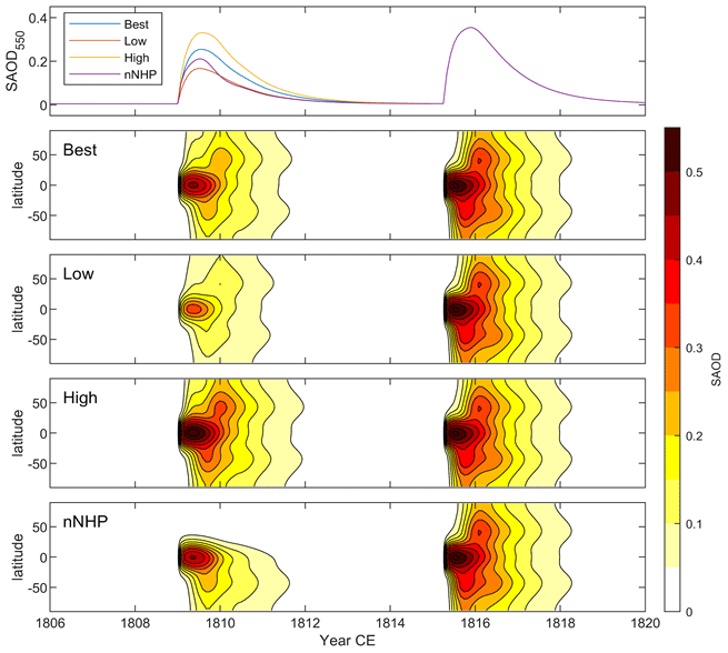
Figure 1Volcanic radiative forcing. Global stratospheric aerosol optical depth (SAOD) at 0.55 µm based on eVolv2k VSSI estimates (Toohey and Sigl, 2017) and calculation with the volcanic forcing generator EVA (Toohey et al., 2016) for the four different forcing scenarios (“Best”, “Low”, “High”, and “nNHP”) for the 1809 eruption and the Best forcing scenario for the Mt. Tambora eruption. Bottom: spatial and temporal distribution of a zonal-mean stratospheric SAOD for the four experiments.
Time series of global-mean and zonal-mean SAOD at 0.55 µm for the different 1809 aerosol forcing scenarios discussed above are shown in Fig. 1, together with the Best scenario after the Mt. Tambora eruption. Peak global-mean SAOD values following the 1809 eruption range from 0.17 to 0.33 from the Low to High scenarios, roughly corresponding to forcing from a little stronger than that from the 1991 Pinatubo eruption to a little weaker than the 1815 Mt. Tambora eruption, respectively. The nNHP scenario produces a global-mean SAOD that peaks at a value of 0.21, i.e., between the Low and Best scenarios, and decays in a manner very similar in magnitude to the Low scenario. The latitudinal spread of aerosol is relatively evenly split between the NH and SH in the Best, Low, and High scenarios, with offsets in the timing of the peak hemispheric SAOD resulting from the parameterized seasonal dependence of stratospheric transport in EVA. After the removal of aerosol mass from the NH extratropics in the construction of the nNHP scenario, the SAOD is predictably negligible in the NH extratropics, and a strong gradient in SAOD is produced at 30∘ N.
2.1.3 Experiments
We have performed ensemble simulations of the early 19th century with the MPI-ESM1.2-LR for each of the four forcing scenarios for the 1809 eruption (Best, High, Low, and nNHP). All simulations also include the eVolv2k Best forcing estimate for the Mt. Tambora eruption from 1815 onwards. Related experiments using a range of different forcing estimates for the 1815 Mt. Tambora eruption were used in Zanchettin et al. (2019) and Schurer et al. (2019) to investigate the role of volcanic forcing uncertainty in the climate response to the 1815 Mt. Tambora eruption, in particular the “year without summer” in 1816. For each experiment we have produced 10 realizations branched off every 100 to 200 years from an unperturbed 1200-year-long pre-industrial control run (constant forcing, excluding background volcanic aerosols) to account for internal climate variability. All simulations were initialized on 1 January 1800 with constant pre-industrial forcing except for stratospheric aerosol forcing.
2.2 Data
2.2.1 Temperature reconstructions
Tropical temperature reconstructions
In our study, we compare three different sea surface temperature (SST) reconstructions with the MPI-ESM simulations. The temperature reconstruction TROP is a multi-proxy tropical (30∘ N–30∘ S, 34∘ E–70∘ W) annual SST reconstruction between 1546 and 1998 (D'Arrigo et al., 2009). TROP consists of 19 coral, tree-ring, and ice-core proxies located between 30∘ N and 30∘ S. The records were selected on the basis of data availability, dating certainty, annual or higher resolution, and a documented relationship with temperature. It shows annual- to multi-decadal-scale variability and explains 55 % of the annual variance in the most replicated period of 1897–1981. Further, 400-year-long spatially resolved tropical SST reconstructions for four specific regions in the Indian Ocean (20∘ N–15∘ S, 40–100∘ E), the western (25∘ N–25∘ S, 110–155∘ E) and eastern Pacific (10∘ N–10∘ S, 175∘ E–85∘ W), and the western Atlantic (15–30∘ N, 60–90∘ W) were compiled by Tierney et al. (2015) based on 57 published and publicly archived marine paleoclimate datasets. The four regions were selected based on the availability of nearby coral sampling sites and an analysis of spatial temperature covariance. An even more regionally specific SST reconstruction was developed by D'Arrigo et al. (2006) for the Indo-Pacific warm pool region (15∘ S–5∘ N, 110–160∘ E) using annually resolved teak-ring-width and coral δ18O records. This September–November mean SST reconstruction dates from 1782–1992 CE and explains 52 % of the SST variance in the most replicated period. This record was used in the D'Arrigo et al. (2009) TROP reconstruction.
Northern Hemisphere extratropical temperature reconstruction
We compare our climate simulations of the early 19th century with four near-surface air temperature (SAT) reconstructions, which have all been used to assess the impacts of volcanic eruptions on surface temperature. The N-TREND (Northern Hemisphere Tree-Ring Network Development) reconstructions (Wilson et al., 2016; Anchukaitis et al., 2017) are based on 54 published tree-ring records and use different parameters as proxies for temperature. A total of 11 of the records are derived from ring width (RW), 18 are from maximum latewood density (MXD), and 25 are mixed records which consist of a combination of RW, MXD, and blue intensity (BI) data (see Wilson et al., 2016, for details). The N-TREND database domain covers the NH midlatitudes between 40 and 75∘ N, with at least 23 records extending back to at least 978 CE. Two versions of the N-TREND reconstructions are used herein. N-TREND (N), detailed in Wilson et al. (2016), is a large-scale mean composite May–August temperature reconstruction derived from averaging the 54 tree-ring records weighted to four longitudinal quadrats, with separate nested calibration and validation performed as each shorter record is removed back in time. N-TREND (S), detailed in Anchukaitis et al. (2017), is a spatial reconstruction of the same season derived by using point-by-point multiple regression (Cook et al., 1994) of the tree-ring proxy records available within 1000 to 2000 km of the center point of each 5 × 5∘ instrumental grid cell. For each gridded reconstruction a similar nesting procedure was used as Wilson et al. (2016). Herein, we use the average of all the grid point reconstructions for the periods during which the validation reduction of error (RE – Wilson et al., 2016) was greater than zero. The NVOLC reconstruction (Guillet et al., 2017) is an NH summer temperature reconstruction over land (40–90∘ N) composed of 25 tree-ring chronologies (12 MXD, 13 TRW) and three isotope series from Greenland ice cores (DYE3, GRIP, Crete). NVOLC was generated using a nested approach and includes only chronologies which encompass the full time period between today and the 13th century. The temperature reconstruction by Schneider et al. (2015) is based on 15 MXD chronologies distributed across the NH extratropics. All the temperature reconstructions show distinct short-time cooling after the largest eruptions of the Common Era. However, Schneider et al. (2017) point to a notable spread in the post-volcanic temperature response across the different reconstructions. This has various possible explanations, including the different parameters used, the spatial domain of the reconstruction, the method(s) used for detrending, and choices made in the network compilations.
2.2.2 Observed temperatures
Surface air temperature from English East India Company ship logs
Brohan et al. (2012) compiled an early observational dataset of weather and climate between 1789 and 1834 from records of the English East India Company (EEIC), which are archived in the British Library. The records include 891 ships' logbooks of voyages from England to India or China and back containing daily instrumental measurements of temperature and pressure, as well as wind-speed estimates. Several thousand weather observations could be gained from these ship voyages across the Atlantic and Indian oceans, providing a detailed view of the weather and climate in the early 19th century. Brohan et al. (2012) found that mean temperatures expressed a modest decrease in 1809 and 1816 as a likely consequence of the two large tropical volcanic eruptions during the period. Following Brohan et al. (2012), here we calculate temperature anomalies from the SAT measurements recorded in the EEIC logs. We account for the relatively sparse and irregular spatial and temporal sampling by computing for each measurement its anomaly from the HadNMAT2 night marine air temperature climatology (Kent et al., 2013). The SAT anomalies were then binned according to the month, year, and location and averaged. We present the data as mean temperature anomalies for the tropics (20∘ S to 20∘ N) in monthly or annual means. To quantify the impact of the 1809 eruption, anomalies are referenced to the 1800–1808 time period.
Station data
Climate model output is compared with monthly temperature series from land stations that cover the period 1806–1820 from a number sources, as compiled in Brönnimann et al. (2019b). The sources include data available electronically from the German Weather Service (DWD), the Royal Dutch Weather service (KNMI), the International Surface Temperature Initiative (Rennie et al., 2014), and the Global Historical Climatology Network (Lawrimore et al., 2011). In addition, we added nine series digitized from the compilation of Friedrich Wilhelm Dove that were not contained in any of the other sources (Dove, 1838, 1839, 1842, 1845). Of the 73 series obtained, 20 had less than 50 % data coverage within the period 1806 to 1820 and were thus not further considered. The remaining 53 time series (see Appendix Table A1) were deseasonalized based on the 1806–1820 mean seasonal cycle and grouped by region (see Appendix Table A2).
2.3 Analysis of model output
Post-eruption climatic anomalies in the volcanically forced ensembles are compared with both anomalies from the control run (describing the range of intrinsic climate variability) and with anomalies from a set of proxy-based reconstructions and instrumental observations, providing a reference or target to evaluate the simulation under both volcanically forced and unperturbed conditions. Comparison between the volcanically forced ensembles and the control run is based on the generation of signals in the control simulation analogous to the post-eruption ensemble-mean and ensemble-spread anomalies. In practice, a large number (1000) of surrogate ensembles is sampled from the control run, each identified by a randomly chosen year as a reference for the eruption. Ensemble means and spreads (defined by 5th and 95th percentiles) of such surrogate ensembles provide an empirical probability distribution that is used to determine the range of intrinsic variability, which is illustrated by the associated 5th–95th percentile ranges. Differences between the volcanically forced ensembles and the surrogate ensembles are tested statistically through the Mann–Whitney U test (following, e.g., Zanchettin et al., 2019). When the ensembles are compared with a one-value target, either an anomaly from reconstructions and observations or a given reference (e.g., zero), the significance of the difference between the ensemble and the target is determined based on whether the latter exceeds a given percentile range from the ensemble (e.g., the interquartile or the 5th–95th percentile range) or, alternatively, based on a t test.
Integrated spatial analysis between the simulations and the N-TREND (S) gridded reconstruction is performed through a combination of the root mean square error (RMSE) and spatial correlation. Both metrics are calculated by including grid points in the reconstructions that correspond to the proxy locations and interpolating the model output to those locations with a nearest-neighbor algorithm. The relative contribution of each location is weighted by the cosine of its latitude to account for differences in the associated grid cell area.
In proxy and instrumental records of tropical temperatures, cooling in the years 1809–1811 is generally on par with that after the 1815 Mt. Tambora eruption. Based on annually resolved temperature-related records from corals, TRs, and ice cores, D'Arrigo et al. (2009) report peak tropical cooling of −0.77 ∘C in 1811 compared to −0.84 ∘C in 1817 (Fig. 2a). Tropical SST variability is modulated by El Niño–Southern Oscillation (ENSO) variability such as neutral to La Niña-like conditions in 1810 and El Niño-like ones in 1816 (Li et al., 2013; McGregor et al., 2010). The lagged response to the 1809 and 1815 eruptions in the TROP reconstruction is therefore most likely a result of an overlaying El Niño signal. Removing the ENSO signal from the TROP reconstructions led to a shift of maximum post-volcanic cooling from 2 years after the eruption to 1 year (D'Arrigo et al., 2009). A clear signal is found in reconstructed Indo-Pacific warm pool SST anomalies from the post-1809 period of 1809–1812, with values of −0.28, −0.73, −0.76, and −0.79 ∘C compared to −0.30, −0.51, and −0.51 ∘C for the post-Tambora period of 1815–1817 (D'Arrigo et al., 2006). Chenoweth (2001) reports pronounced tropical cooling from ship-based marine SAT measurements in 1809 (−0.84 ∘C) that is similar to that in 1816 (−0.81 ∘C). More recent analysis of a larger set of ship-based marine SAT records from the EEIC by Brohan et al. (2012) suggests a more modest cooling for the two early 19th century eruptions of about 0.5 ∘C (Fig. 2b). However, the cooling is again found to be of comparable magnitude after the 1809 and 1815 eruptions, and it therefore hints to a tropical location of the 1809 eruption, in agreement with the ice-core data.
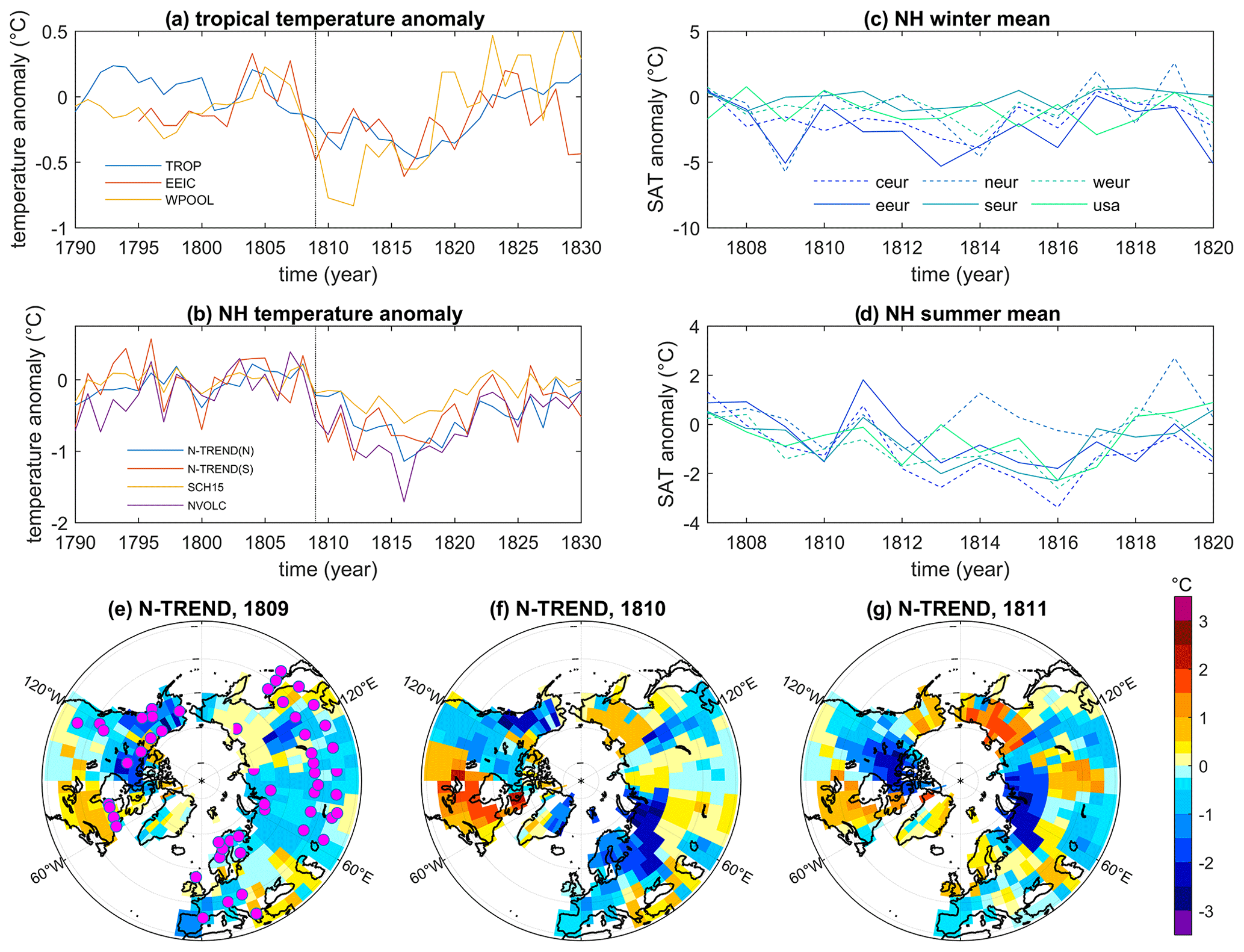
Figure 2Observed and reconstructed temperature anomalies around the 1809 volcanic eruption. (a) Reconstructed tropical (30∘ N–30∘ S, 34∘ E–70∘ W) sea surface temperature (TROP; D'Arrigo et al., 2009), measured tropical marine surface air temperatures from EEIC ship logs (Brohan et al., 2012), and Indo-Pacific warm pool data (D'Arrigo et al., 2006). (b) NH summer land temperatures from four tree-ring-based reconstructions (Wilson et al., 2016, N-TREND (N); Anchukaitis et al., 2017, N-TREND (S); Guillet et al., 2017, NVOLC; Schneider et al., 2015, SCH15). (c–d) Monthly mean NH winter (c) and summer (d) temperature anomalies (∘C) from 53 station datasets averaged over different European regions (central Europe, CEUR: 46.1–52.5∘ N, 6–17.8∘ E; eastern Europe, EEUR: 47–57∘ N, 18–32∘ E; northern Europe, NEUR: 55–66∘ N, 10–31∘ E; southern Europe: 38–46∘ N, 7–13.5∘ E; western Europe, WEUR: 48.5–56∘ N, 6∘ W–6∘ O; and New England, NENG: 41–44∘ N, 73–69∘ W). (e–g) Mean surface temperature anomalies ( ∘C) for boreal summers of 1809 (e), 1810 (f), and 1811 (g) in NH tree-ring data from N-TREND (S) (Anchukaitis et al., 2017). Pink dots in panel (e) illustrate the location of the tree-ring proxies used in the N-TREND reconstructions.
Tree-ring records capture volcanically forced summer cooling very well (e.g., Briffa et al., 1998; Hegerl et al., 2003; Schneider et al., 2015; Stoffel et al., 2015). However, in the NH extratropics, SAT anomalies after 1809 are more spatially and temporally complex compared to the typical post-eruption pattern with broad NH cooling. In tree-ring-based temperature reconstructions for interior Alaska–Yukon (Briffa et al., 1994; Davi et al., 2003; Wilson et al., 2019), 1810 is one of the coldest summers identified over recent centuries. In earlier reconstructions of summer SAT in different regions of the western United States (Schweingruber et al., 1991; Briffa et al., 1992), 1810 was shown to be the third-coldest summer in the British Columbia–Pacific Northwest region. Likewise, European tree-ring records show cooling after 1809 (e.g., Briffa et al., 1992; Wilson et al., 2016). In contrast, tree-ring networks in certain regions such as eastern Canada show a minimal response after 1809 (Gennaretti et al., 2018).
Based on compilations of regional records, tree-ring-based reconstructions of NH mean land summer SAT show a large spread in hemispheric cooling after the 1809 eruption (Fig. 2b), with anomalies of −0.87, −0.77, −0.21, and −0.15 ∘C in 1810 for the N-TREND (S), NVOLC, N-TREND (N), and SCH15 reconstructions, respectively. Although using the same dataset, the spatial N-TREND (S) and the nested N-TREND (N) reconstructions show quite different behavior. In N-TREND (S), the nature of the spatial multiple regression modeling biases the input records to those that correlate most strongly with local temperatures, which, when available, are likely MXD data. In all four reconstructions, NH temperature does not return to the climatological mean after an initial drop in 1810 but remains low or even exhibits a continued cooling trend until the Mt. Tambora eruption in 1815 (Schneider et al., 2015). The spatial variability of the reconstructed NH extratropical temperature response to the 1809 eruption is illustrated in Fig. 2e, f, and g based on the spatially resolved N-TREND (S) reconstruction (Anchukaitis et al., 2017), displaying zonal oscillations consistent with a “wave-2” structure that are especially evident in 1810 but already appreciable in 1809. This hemispheric structure is in contrast with the relatively uniform cooling seen in tree-ring records for Tambora (Fig. S3) and indeed for many of the largest eruptions of the past millennium (Hartl-Meier et al., 2017).
Information about regional and seasonal mean NH temperature anomalies in the early 19th century can be obtained from different station data across Europe and from New England (Fig. 2c, d). In NH winter the measurements reflect the high variability of local-scale weather (Fig. 2c). Warm anomalies, an indication for post-eruption “NH winter warming”, are clearly visible in 1816/1817 in the second winter after the Mt. Tambora eruption in 1815. Northern Europe shows the largest warm anomaly for all regions (about 3 ∘C). Warm NH winter anomalies between 1.5 and 2 ∘C are seen in the winter 1809/1810 over northern and eastern Europe and over New England. Strong cooling, however, is found for the 1808/1809 winter in northern and central Europe. NH summer temperature anomalies are less variable than in winter (Fig. 2d). A local distinct cooling is found in the “year without summer” in 1816 over all regions except northern Europe, where it occurs a year later. The cooling after the 1809 eruption is not so pronounced as after the Mt. Tambora eruption in 1815.
In general the station data support the spatial distribution of the reconstructed near-surface temperature anomalies derived from tree-ring data. They show a local minimum over northern, eastern, and southern Europe in NH summer 1810, which does not appear over western and central Europe and New England. The warm anomalies of the order of 2 ∘C, which are found in summer 1811 over eastern Europe, are not captured by the N-TREND spatial reconstruction, although some slight warming is seen in the data over eastern Poland, Belarus, and the Baltic states.
4.1 Simulations
Firstly, we compare the simulated evolutions of monthly mean near-surface (2 m) air temperature anomalies between the four experiments globally, in the tropics, and in the NH extratropics (Fig. 3). Ensemble-mean global-mean temperature anomalies grow through 1809 and reach peak values through 1810 in all experiments before decaying towards climatological values (Fig. 3a). Peak cooling reaches around 1.0 ∘C in the High experiment compared to 0.5 ∘C in the Low and nNHP experiments. Peak temperature anomalies across the experiments correlate with the magnitude of prescribed AOD (Fig. 1a), and the responses are qualitatively consistent with expectations; the AOD for the Low and nNHP experiments, which is similar in magnitude to that from the observed 1991 Pinatubo eruption, leads to global-mean temperature anomalies also similar to those observed after Pinatubo. Global ensemble-mean near-surface temperature anomalies are close together in Low and nNHP over boreal summer but differ for boreal winter when the intrinsic variability is higher. Low is the only experiment for which large-scale temperatures return to within the 5th–95th percentile range of the control run before the Mt. Tambora eruption in 1815. Global-mean temperature anomalies of the other three experiments return only to within the 5th–95th percentile range of unperturbed variability by 1815. As expected, almost no significant near-surface temperature anomalies are found for the nNHP simulation in the NH extratropics except a few months in spring and autumn 1813 (Fig. 3b). The nNHP ensemble-mean values stay within the interquartile range of the control run but show a slight negative trend between 1809 and 1815. The nNHP is also the only experiment in which the NH extratropical summer of 1814 is colder than the summer of 1809. Internal variability is relatively high in the NH extratropics, in particular in NH winter, spanning more than 1.5 ∘C. So, even the ensemble-mean near-surface temperature anomalies for the Best and High experiments almost reach the 5th–95th percentile range of the control run in the first post-volcanic winters. Peak cooling appears for all experiments except nNHP in the summer 1810. In the tropics, the Best, High, and nNHP experiments are outside the 5th–95th percentile range in the first 4 post-volcanic years, while Low exceeds the 5th–95th percentile range only for 2 years (Fig. 3c).
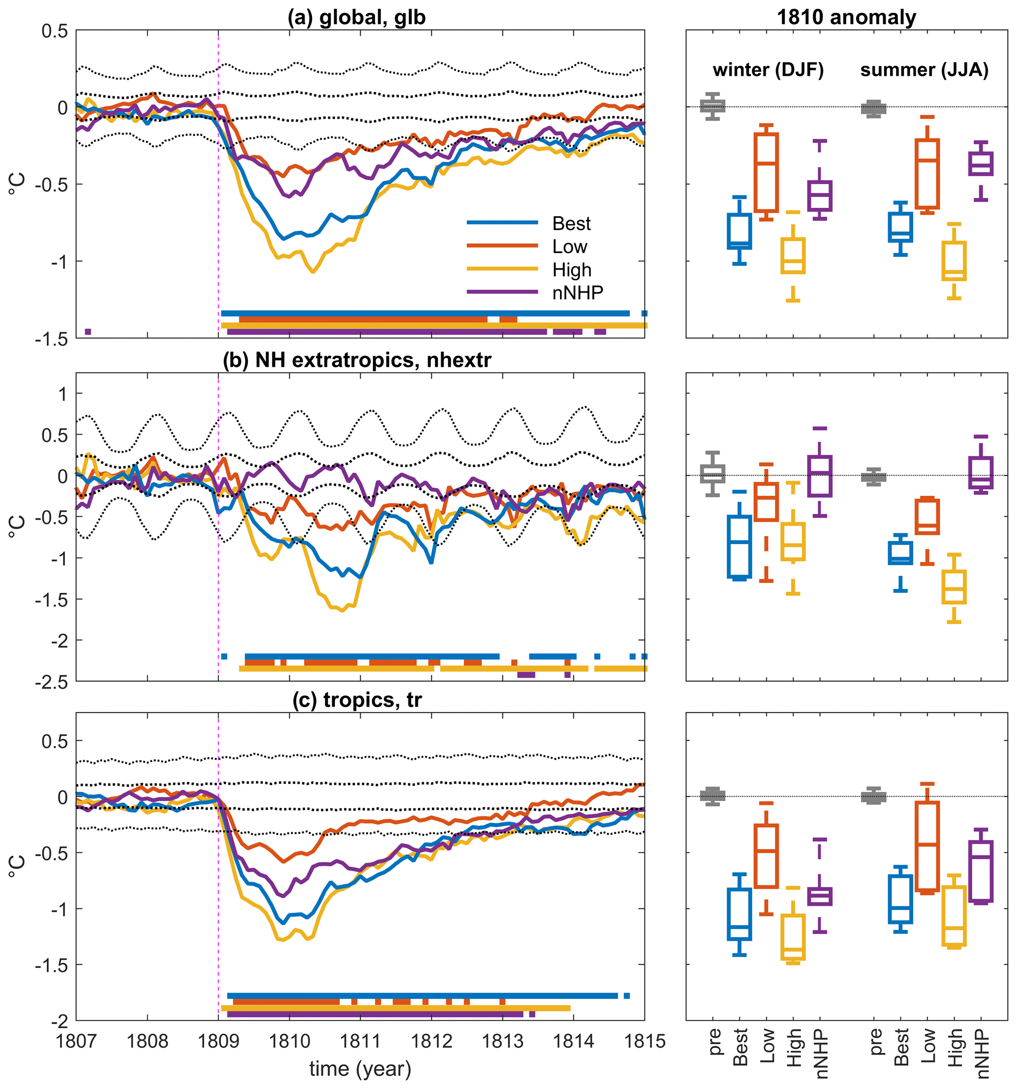
Figure 3Global, tropical, and extratropical temperature anomalies. Left: simulated ensemble-mean monthly anomalies of (a) global, (b) extratropical Northern Hemisphere, and (c) tropical averages of near-surface air temperature with respect to the pre-eruption (1800–1808) climatology. All data are deseasonalized using the respective annual average cycle from the control run. Thick (thin) black dashed lines are the 5th–95th percentile intervals for signal occurrence in the control run for the ensemble mean (ensemble spread). Bottom bars indicate periods when an ensemble member's monthly mean temperature (color code as for the time series plots) is significantly different (p=0.05) from the control run according to the Mann–Whitney U test. Right: ensemble distributions (median as well as 25th–75th and 5th–95th percentile ranges) of seasonal mean anomalies for the first post-eruption winter (1809–1810, DJF) and summer (1810, JJA) following the 1809 eruption as well as for the pre-eruption period (1800–1808).
The ensemble distributions for the seasonal mean of winter 1809/1810 and summer 1810 illustrate the differences between the four experiments not only in the mean anomaly but also for the ensemble spread (Fig. 3d–f). While, for example, in summer 1810 the global and tropical ensemble means of the Low and nNHP experiments are quite close, the ensemble spread is much larger in Low compared to nNHP. The Low experiment generally has the largest ensemble spread independent of season and hemispheric scale. The clearest separation between the experiments appears in the NH extratropics in summer 1810 (Fig. 3f), in line with Zanchettin et al. (2019), who show with a k-means cluster analysis on a large ensemble that forcing uncertainties can overwhelm initial condition spread in boreal summer.
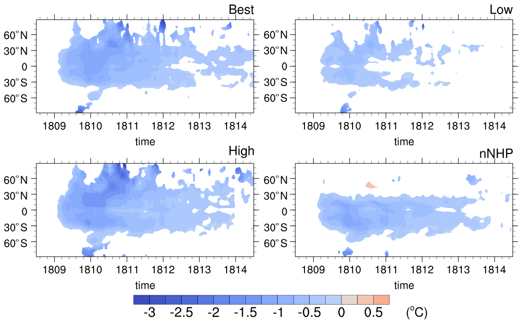
Figure 4Simulated ensemble-mean zonal-mean near-surface air temperature anomalies (∘C) for the four MPI-ESM experiments. Only anomalies exceeding 1 standard deviation of the control run are shown. Anomalies are calculated with respect to the pre-eruption (1800–1808) climatology.
A more detailed spatial distribution of the simulated temporal evolution of post-volcanic surface temperature anomalies is seen in the Hovmöller diagram in Fig. 4. It shows that in all four experiments a multiannual surface temperature response is found in the tropics (30∘ S–30∘ N). In the inner tropics, the cooling disappears after 1.5 years in the Low experiment and 2 to 3 years later in the Best, High, and nNHP experiments. In the subtropics, a significant surface cooling signal is found over the ocean until 1815 in Best and High, while over land no significant cooling appears in 1814 (Fig. S4). A strong cooling signal is found in the NH extratropics in the Best, Low, and High experiments in summer 1810 as well as in the High and to a small extent also in the Best experiment in summer 1811. In nNHP no surface cooling is detectable over the NH extratropics in the first 4 years after the eruption, consistent with the prescribed volcanic forcing (see Fig. 1). However, a cooling anomaly is apparent around 60∘ N in summer 1813, which is seen in the zonal mean over the ocean (Fig. S4) and likely due to decreased poleward ocean heat transport. Significant cooling south of 30∘ S appears only in austral spring 1809.
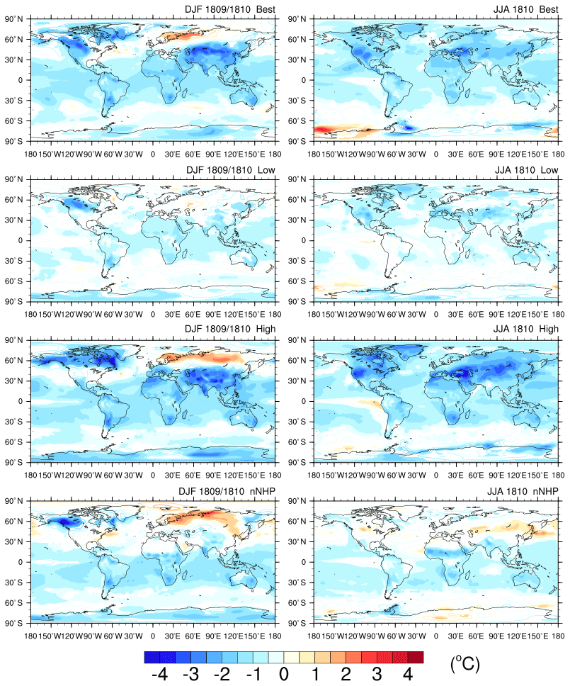
Figure 5Simulated ensemble-mean near-surface air temperature anomalies for the first winter (1809/1810) and the second summer (1810) after the 1809 eruption for the four different MPI-ESM simulations. Shaded regions are significant at the 95 % confidence level according to a t test. Anomalies are calculated with respect to the period 1800–1808.
Figure 5 shows the spatial near-surface air temperature anomalies for the first boreal winter (1809/1810) and the second boreal summer (1810) after the 1809 eruption for the four experiments. In general, the cooling is strongest over the NH continents in all experiments, revealing a strong cooling pattern over Alaska, Yukon, and the Northwest Territories in the first post-eruption winter. In the Best and High experiments, relatively strong cold anomalies are found over the central Asian dry highland regions around 40∘ N from the Hindu Kush in the west to the Pacific, while the Low and nNHP experiments show a small yet significant cooling over India and southeastern China. In boreal winter a significant warming is visible over Eurasia in all experiments except for Low, wherein warming anomalies are instead found over the polar ocean, and it is most pronounced in the High experiment but also quite extensive in nNHP. Such an NH winter warming pattern is known to be induced by atmospheric circulation changes (e.g., Wunderlich and Mitchell, 2017; DallaSanta et al., 2019) and can occur in post-eruption winters as a dynamic response to the enhanced stratospheric aerosol layer when it displays a highly variable amplitude of local anomalies (Shindell et al., 2004). Accordingly, in our simulations the Eurasian winter warming pattern consists of one or two areas with positive temperature anomalies centered over various locations between Fennoscandia and the Central Siberian Plateau in the different simulations. Significant cooling, albeit of different strength, is found in the NH extratropics in boreal summer in the three symmetric forcing experiments (Best, High, Low). However, while all of them show significant negative temperature anomalies over the North American continent with a local maximum over California and also cooling over Greenland, no significant anomalies are seen in the Low experiment over Fennoscandia. Except for some small regions (Finland, the Kola Peninsula, and western Alaska), no significant cooling is found in nNHP in the NH extratropics in boreal summer. The spatial distribution of the forcing can impact the latitudinal position of peak surface cooling, which in turn can lead to a shift of the Intertropical Convergence Zone (e.g., Haywood et al., 2013; Pausata et al., 2020). This is clearly visible in the cold anomaly belt over the Sahel region in the asymmetric forcing experiment nNHP. Significant warm anomalies are detectable in a small band that extends from the Caspian Sea in the west to Japan in the east. Cooling over the ocean is weaker and mostly confined in the tropical belt between 30∘ S and 30∘ N. The High experiment is the only experiment in which a significant El Niño-type anomaly is seen over the Pacific Ocean in boreal summer 1810, while in the other three experiments a slight but non-significant warming appears off the coast of South America. Looking at the relative SST anomalies as calculated after Khodri et al. (2017), an El Niño-type anomaly is seen for all four scenarios in boreal summer 1810, while in winter 1809/1810 a significant warming anomaly appears in the central tropical Pacific in all experiments except the Best experiment (Fig. S5).
The substantial differences found in the post-eruption evolution of continental and subcontinental climates reflect the variety of climate responses produced by different combinations of internal climate variability and forcing structure. In this regard, post-eruption anomalies of selected dominant modes of large-scale atmospheric circulation in the Northern Hemisphere and the tropics, including the Pacific–North American pattern, the North Atlantic Oscillation, the North Pacific Index, and the Southern Oscillation, yield a spread of responses within individual ensembles that is often as large as the range of pre-eruption variability. Further, response distributions generated by different forcings in some cases do not overlap (see Fig. S1).
4.2 Model–data comparison
4.2.1 Tropics
A multiannual cooling signal is found in the MPI-ESM simulations in the tropical region after the unidentified 1809 eruption (Figs. 3 and 4). The same signature is detected in the English East India Company (EEIC) ship-based surface air temperature anomaly annual means (Brohan et al., 2012) as well as in tropical SST reconstructions (TROP; D'Arrigo et al., 2009) and the Indo-Pacific warm pool (D'Arrigo et al., 2006) in Fig. 6. The simulated ensemble-mean temperatures (Fig. 6a) bracket the observed anomaly in the EEIC data in 1809, with the observed value falling between the results of the Low and nNHP forcing experiments. In 1810–1812, the cooling in the Best, High, and nNHP experiments is stronger than that observed, and therefore the results from the Low experiment are generally the most consistent with the shipborne measurements (Fig. 6a). When the model results are sampled at the locations and times of the EEIC measurements (Fig. S6), the mean negative temperature anomalies in 1809 are 10 %–30 % smaller, with the Best, High, and nNHP experiments all producing anomalies similar to that of the EEIC measurements. For the 1810–1812 period, the sampling makes little difference compared to the full tropical average, with the Best, High, and nNHP experiments all showing larger negative temperature anomalies than the EEIC measurements. A comparison of TROP with our four experiments reveals that all experiments lie within the 5th–95th percentile interval of the TROP reconstruction, although the reconstructed SST response appears to be dampened in comparison to the model experiments (Fig. 6b). Although the long-term trends of TROP and the model experiments are in general agreement, the dampened post-volcanic cooling could reflect autocorrelative biases in the proxies (Lücke et al., 2019). Detailed scrutiny of high-resolution tropical SST proxies and their potential biases to robustly reflect volcanically forced cooling has not been made in the same way as has been performed for tree-ring archives over the last decade (Anchukaitis et al., 2012; D'Arrigo et al., 2013; Esper et al., 2015; Franke et al., 2013; Lücke et al., 2019). A similar behavior is found for the Indonesian warm pool (Fig. 6c). However, in contrast to the whole tropics, the differences between the different forcing experiments are much smaller for the warm pool region compared to the wider tropical regions, and the volcanic signal is more pronounced in the reconstructed SST, at least for the unidentified 1809 eruption.
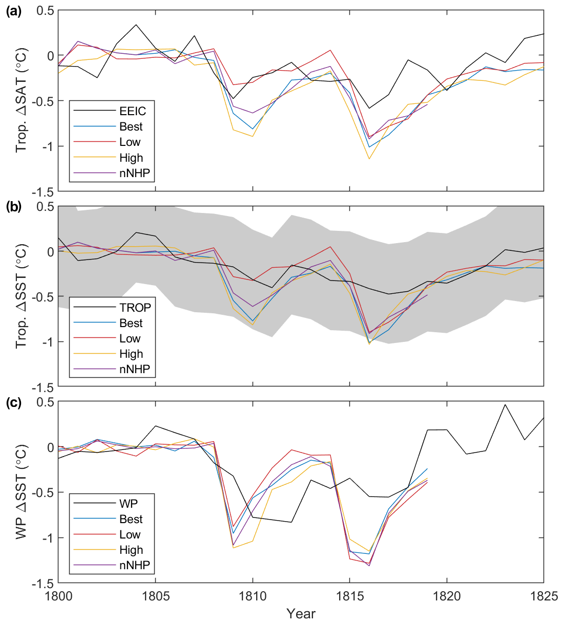
Figure 6Comparison of tropical temperatures anomalies. Comparison of the MPI-ESM simulations with (a) tropical and annual mean (30∘ N–30∘ S) surface air temperature from shipborne measurements of the English East India Company (EEIC; Brohan et al., 2012), (b) annual mean tropical sea surface temperature (SST) reconstruction (TROP; D'Arrigo et al., 2009) over the tropical Indo-Pacific (30∘ N–30∘ S, 34∘ E–70∘ W), and (c) seasonal mean (September–November) SST reconstruction (D'Arrigo et al., 2006) anomalies over the Indonesian warm pool (WP; 15∘ S–5∘ N, 110–160∘ E). The black line represents the observed or reconstructed data in all panels, while the colored lines represent ensemble means of the respective model simulations. The grey shaded regions in (b) indicate the 95 % confidence interval of the reconstruction. Anomalies are taken with respect to the years 1800 to 1808.
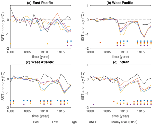
Figure 7Coral–SST comparison. Comparison of reconstructed tropical annual mean SST (Tierney et al., 2015) with the MPI-ESM experiments over the (a) eastern Pacific (10∘ N–10∘ S, 175∘ E–85∘ W), (b) western Pacific (25∘ N–25∘ S, 110–155∘ E), (c) western Atlantic (15–30∘ N, 60–90∘ W), and (d) Indian (20∘ N–15∘ S, 40–100∘ E) oceans. Black solid line: SST reconstruction; colored lines: ensemble means of the model simulations. Anomalies are taken with respect to the years 1800 to 1808. The squares on the bottom of each panel indicate years when the observation lies outside the simulated ensemble range (color code as for the ensemble mean).
Tierney et al. (2015) provided coral-based reconstructions of tropical SSTs for four different ocean regions: the Indian Ocean, the western and eastern Pacific, and the western Atlantic. Comparison of our four experiments with the coral-based reconstructions reveals quite different behavior and simulation–reconstruction agreement across the various regions (Fig. 7). For the eastern Pacific region, the reconstruction and the MPI-ESM simulations are not inconsistent with each other over the 1809 period, showing substantially high variability (Fig. 7a) that reflects the influence of both ENSO and volcanic cooling. A clear volcanic signal is therefore found in the four experiments only for the Mt. Tambora eruption, while for the 1809 eruption, the High and Best experiments show a distinct cooling in 1809 and nNHP in 1811. In contrast to the eastern Pacific, variability in the western Pacific is rather small (Fig. 7b). In all four experiments a clear volcanic signal is visible in the simulated ensemble-mean SST anomaly after the 1809 eruption and the Mt. Tambora eruption, whereas only a weak signal appears for both eruptions in the reconstruction. Interestingly, in the western Atlantic, two distinct positive SST anomalies appear in the reconstructions in the aftermath of the unidentified 1809 and the Mt. Tambora eruption, while the MPI-ESM simulations show cooling (Fig. 7c). Reasons for the anticorrelated behavior are not obvious per se and may be related to changes in either ocean circulation or climate factors other than SST that influence the coral record, such as salinity and precipitation. In the reconstruction, the Indian Ocean is the only region that displays a peak cold anomaly after the Mt. Tambora eruption, but the magnitude of this cooling is comparable to an apparent cooling in 1807. A clear reference to the Mt. Tambora eruption is therefore difficult to establish. No large cooling is found in the coral data after 1809 over the Indian Ocean (Fig. 7d).
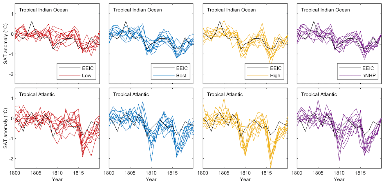
Figure 8Annual mean surface air temperature anomalies from shipborne measurements of the English East India Company (EEIC) (Brohan et al., 2012) over the tropical Indian and Atlantic oceans (black line) compared to similarly sampled model simulations from the Low, Best, High, and nNHP forcing ensembles as labeled. Anomalies are taken with respect to the years 1800 to 1808.
Instrumental measurements from the tropical region are sparse, and no continuous temperature record covering the early 19th century exists. Figure 8 shows a comparison between the model simulations and ship-based surface air temperature measurements from the tropical Atlantic and Indian oceans. For each ocean basin, the model output is sampled at the locations and times of the ship measurements. For the Indian Ocean, observed temperature anomalies after 1809 are within the model ensemble spread of all the model ensembles. The model response in the Indian Ocean is quite variable for the Low forcing experiment, with some members showing no apparent cooling and others with cooling of up to 0.9 ∘C. Overall, observed Indian Ocean temperature anomalies are on the lower edge of the Low ensemble. For the Best, High, and nNHP experiments, the simulated cooling over the Indian Ocean is more consistent across individual simulations, with the ensemble spread enveloping the observed temperature time series. While Low forcing is not inconsistent with the observed Indian ocean temperatures, Best, High, and nNHP appear more likely scenarios. In the tropical Atlantic, the observed cooling after the 1809 eruption is slightly stronger than for Mt. Tambora and slightly stronger than that in the Indian Ocean. The maximum observed cooling in 1809 is roughly within the spread of all the model ensembles. However, while observed tropical Atlantic temperature anomalies are largest in 1809, the simulated cooling usually peaks in 1810. In 1810, the observed cooling is less than simulated in the Best ensemble and smaller than all but one of the individual simulations in the High ensemble. Looking at the years after the Mt. Tambora eruption, simulations and observations agree relatively well in the Indian Ocean, while in the Atlantic, the model simulations overestimate the post-Tambora cooling. Since satellite observations of the aerosol cloud from the 1991 eruption of Pinatubo show that aerosol quickly spreads uniformly across the tropics, it is unlikely that aerosol forcing from the 1809 eruption would be significantly different between the tropical Indian and Atlantic Ocean basins. Therefore, differences in temperature response in the model between the two regions seems more likely to be related to model sensitivity, which might particularly be linked to differences in ocean circulation and/or mixed layer depth.
4.2.2 Northern Hemisphere extratropics
Figure 9 shows a comparison between the model experiments with four NH summer land near-surface temperature reconstructions from tree-ring records, including the nested N-TREND (N) (Wilson et al., 2016) and the spatial N-TREND (S) reconstruction (Anchukaitis et al., 2017). To ensure comparability between the reconstructions and the model results, the data are expressed as anomalies with respect to 1800–1808. The High and Best experiments show significantly larger cooling than the reconstructions and are outside the 95 % confidence interval of the N-TREND (N) reconstruction. Simulated SAT anomalies in nNHP are generally smaller than the reconstructions between 1809 and 1815. The best agreement between the ESM simulations and the data after the 1809 eruption is found for the Low experiment. In NH summer 1810 and 1811, the Low experiment matches the reconstructed temperature anomalies from the NVOLC (Guillet et al., 2017) and N-TREND (S) records quite well. Interestingly, the devil really is in the detail. Despite the data richness of this period, the temporal evolution (trend) differs substantially between the different tree-ring reconstructions. In N-TREND (N) the evolution is a step-like temperature decrease with a first step in 1809, followed by a second one in 1812 and persistent low values until 1816. Distinct peak cooling appears in NVOLC and N-TREND (S) in NH 1810, followed by a short recovery phase in 1811 and a drop in 1812, but while summer SAT anomalies stay constant in the NVOLC reconstruction, for N-TREND (S) they start to recover again after 1812. Schneider et al. (2015) show only a small cooling trend between 1809 and 1815. In their reconstruction, temperatures after the 1809 event did not return to their climatological mean after the initial drop but remained low until the Mt. Tambora eruption in 1815. Compared to the reconstructions, the ESM simulations (High, Best, Low) show a very different temporal evolution with a relatively fast recovery after the 1809 eruption to near background conditions, followed by a second cooling peak for the Mt. Tambora eruption starting in 1816. In the MPI-ESM simulations no cooling peak appears in the ensemble mean for the summer of 1812, in contrast to the tree-ring records. The nNHP is the only experiment which shows only a slight cooling trend between 1810 and 1815, appearing closer to Schneider et al. (2015). Between 1813 and 1815, nNHP reveals similar temperature anomalies as the Best and High experiments, while the Low experiment shows less cooling than all other experiments, which even disappears before the onset of the Tambora eruption.
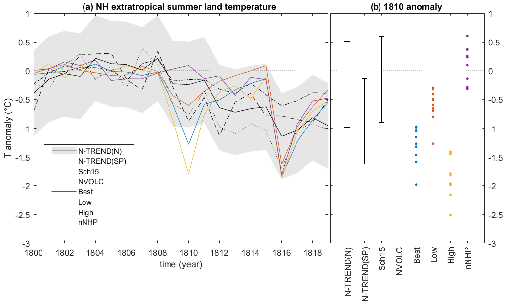
Figure 9Comparison of NH extratropical summer land temperatures. (a) Comparison of simulated NH extratropical (40–75∘ N) summer land temperature anomalies (seasonal and spatial averaged) with four different NH tree-ring-based temperature reconstructions (Wilson et al., 2016, N-TREND (N); Anchukaitis et al., 2017, N-TREND (S); Guillet et al., 2017, NVOLC; Schneider et al., 2015, SCH15). Anomalies are taken with respect to the years 1800–1808. The black lines represent the tree-ring records, and the colored ones represent the ensemble mean of the four MPI-ESM experiments. The shaded grey area indicates the 2σ uncertainty range for N-TREND (N). (b) Comparison for the reconstructed and simulated anomalies for the year 1810. Uncertainty ranges for all reconstructions are based on the 2σ of the N-TREND (N) reconstruction. Simulated anomalies are shown as individual realizations.
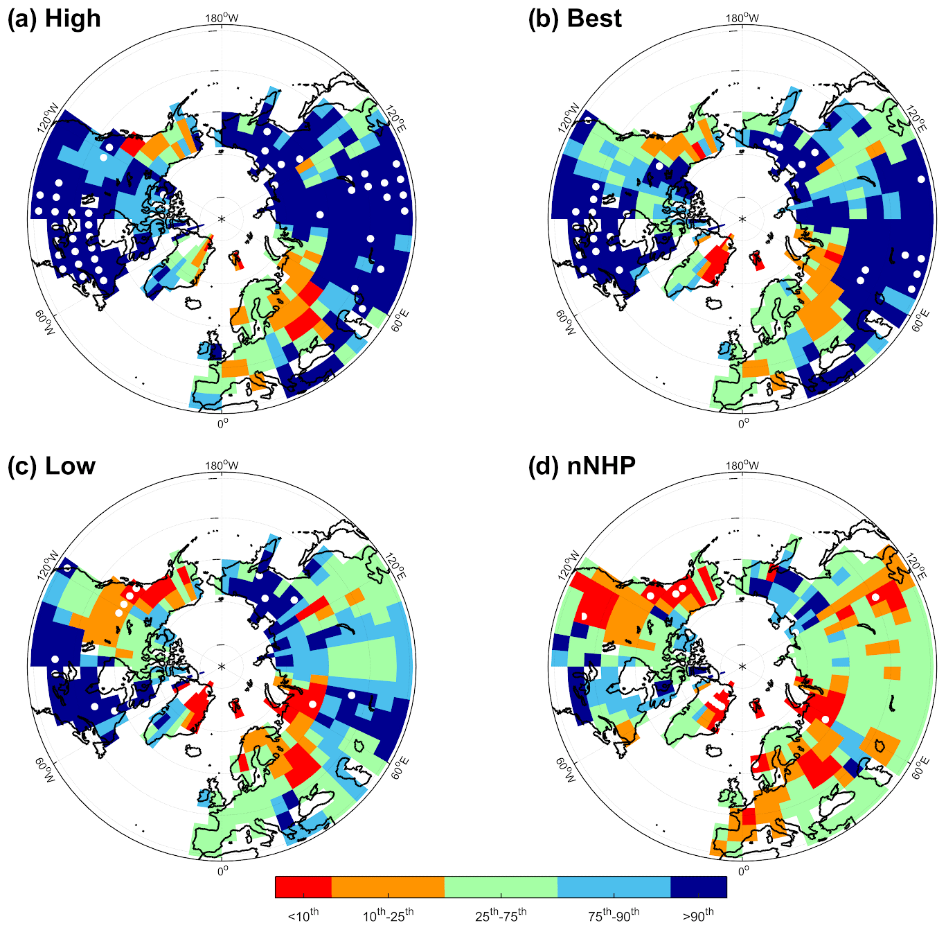
Figure 10Spatial comparison of NH extratropical land temperatures for summer 1810. Statistical comparison of reconstructed surface summer temperatures from N-TREND (S) (Anchukaitis et al., 2017) with the ensemble distributions of the four MPI-ESM ensembles (10 members). Anomalies are for the year 1810 with respect to the 1800–1808 mean. The shading shows, for each grid point, the percentile range of the ensemble simulation in which the reconstructed temperature falls. Green patches indicate that the reconstruction lies in the interquartile range of the simulations and is hence in good agreement with the ensemble. Bluish patches indicate that the reconstruction lies in the higher range of the ensemble; i.e., the majority of simulations are colder than the reconstructions. Reddish patches indicate that the reconstruction lies in the lower range of the ensemble; i.e., the majority of simulations are warmer than the reconstructions. White dots indicate where the reconstruction is an outlier with respect to the distribution of the simulation ensembles, i.e., where the absolute difference between the reconstruction and simulation ensemble mean is greater than 3 times the median absolute deviation of the simulation ensemble.
In Fig. 10, we analyze the spatial patterns of the percentiles of the model ensemble into which the reconstruction falls. If the reconstruction lies in the upper range of the distribution of ensemble members, the reconstructed temperature anomalies are warmer than most simulations; i.e., the majority of simulations are colder than the reconstruction. The High ensemble (Fig. 10a) is in many locations colder than the reconstructions, but the reconstruction from central to northern Europe lies mostly within the interquartile, i.e., the 25th–75th percentile, range of the simulations. This behavior results from the comparison of the variable local cooling in the individual simulations with highly heterogeneous temperature anomalies in the reconstruction (Fig. 2). Only in a few regions (central Europe, western Russia, Alaska) are the simulated temperature anomalies much warmer and the reconstructed one below the 25th percentile. The Best experiment (Fig. 10b) indicates a similar behavior as the High experiment albeit with more regions where the reconstruction lies within the interquartile range of the simulations, e.g., along the west coast of North America. Low (Fig. 10c) and nNHP (Fig. 10d) are the experiments with the best agreement between the simulated and the reconstructed surface temperature anomalies. The nNHP is the experiment in which, compared to the other model experiments, the reconstruction in most locations is within the interquartile range of the simulations and which has the lowest number of locations for which the reconstruction is considered an outlier compared to the simulation ensemble. Overall, the N-TREND (S) reconstruction is colder over eastern Europe and western Russia compared to the simulated surface temperature anomaly distribution in all four experiments and warmer over the eastern part of North America.
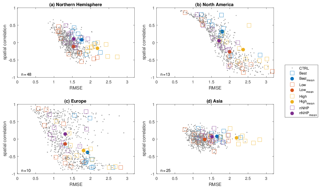
Figure 11Scatterplots of root mean square error (RMSE) versus spatial correlation between simulated NH summer temperature and the N-TREND (S) reconstruction (Anchukaitis et al., 2017) for summer 1810 and different regions: (a) whole Northern Hemisphere, (b) North America (180–60∘W), (c) Europe (60∘ W–60∘ E), (d) Asia (60–180∘ E). Individual model realizations are indicated by squares, and the ensemble mean is indicated by a full dot; small grey dots are for 1000 random samples from the control period (1800 to 1808). Analysis is restricted to grid points for which proxy data are available (number of data used for each region reported in the respective panel).
Another method to compare reconstructed and simulated spatial patterns of temperatures anomalies in summer 1810 is shown in Fig. 11, which illustrates the spatial correlation and root mean square error (RMSE) between the reconstruction and individual ensemble members of each experiment for the whole Northern Hemisphere and three equal-area sections of it. Similar metrics are calculated and shown for individual summers of an unforced control run to illustrate the potential for the model to produce similar spatial structures as a result of natural variability. Perfect agreement between simulated and reconstructed data corresponds to spatial correlation of 1 and RMSE of 0; hence, the best-simulated representations of the reconstructed anomalies are found close to the top-left corner of each panel. A perfect correlation could result from a simulation which had a bias compared to the reconstruction, while RMSE is a result of absolute differences due to spatial differences and biases. Over the entire NH (Fig. 11a) the scatters of all ensembles largely overlap each other and the control run, reflecting the effects of the relatively large internal climate variability. The High and Best ensembles yield ensemble-mean metrics that are at the edge of the control run, with some realizations of the former ensemble being outside the spread of the control run for the NH and Asian regions. Both ensemble simulations are colder than the reconstruction (Fig. 10) for any year of the control run. The Low and nNHP ensembles compare best with the N-TREND (S) reconstruction according to this analysis, especially as they yield the smallest RMSE values regarding both individual realizations and the ensemble mean. The best correlations for the NH, in both the control and the forced experiments, are only 0.5, which reveals that the model does not produce such a spatial pattern as we see in the reconstruction.
Model performance in terms of spatial correlation is especially interesting over North America (Fig. 11b), where a cold–warm zonal dipole is a major characteristic of the N-TREND (S) reconstruction but where the proxy data quality is also not optimal (Anchukaitis et al., 2017). The Low, nNHP, and Best ensembles, as well as the control run, include realizations that yield high spatial correlations over North America. This suggests that such a continental anomaly is consistent with the variability produced naturally by the model. The spread of correlation values over North America is wide, with many realizations showing a strongly negative correlation with the reconstruction, and correlations of the ensemble means are small. There is therefore no evidence from the model that the spatial pattern of temperature anomalies over North America is a specific response to the volcanic aerosol forcing. The results for Europe (Fig. 11c) are similar to those of North America, with a handful of simulations from the Low and nNHP experiments showing the highest correlation with the reconstruction but no clear improvement of the forced simulations in general compared to the control run. The range of correlations for the ensembles and the control run is smaller over Asia (Fig. 11d) than in the other considered regions; i.e., no realizations show strong positive (or negative) correlations with the reconstruction, as ensembles, except nNHP, yield anomalies that are too cold, especially over eastern Siberia, that contrast with the weak anomalies reconstructed there (Fig. 10). This is most likely related to a substantial data quality issue, as the tree-ring data, especially for central Asia, are solely based on TRW data (Wilson et al., 2016). However, we also cannot rule out the possibility of a model bias, as the climatological mean state of near-surface air temperature in the MPI-ESM-LR over central Asia deviates from ERA-Interim by a few degrees (Müller et al., 2018).
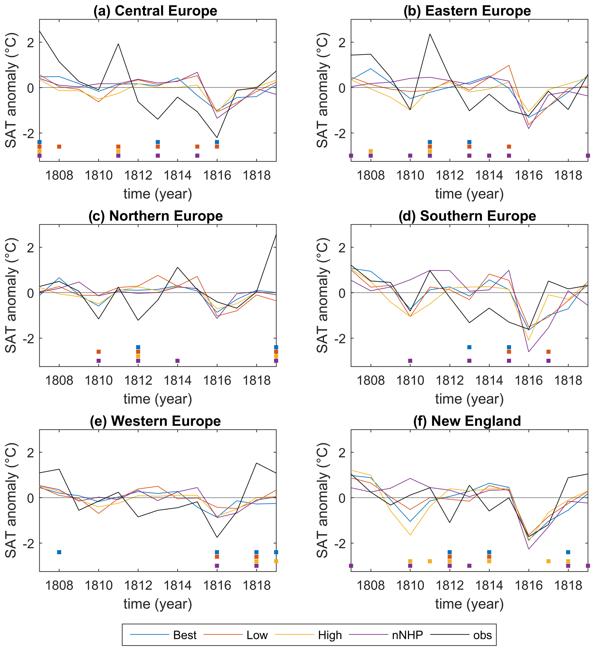
Figure 12Seasonal mean near-surface NH summer temperature anomalies (∘C) with station data averaged over different regions: (a) central Europe (46.1–52.5∘ N, 6–17.8∘ E), (b) eastern Europe (47–57∘ N, 18–32∘ E), (c) northern Europe (55–66∘ N, 10–31∘ E), (d) southern Europe (38–46∘ N, 7–13.5∘ E), (e) western Europe (48.5–56∘ N, 6∘ W–6∘ E), and (f) New England (41–44∘ N, 73–69∘ W). The black line represents measurements, and the colored lines represent the ensemble mean of the model simulations. The squares on the bottom of each panel indicate years when the measurement lies outside the simulation ensemble range (color code as for the ensemble mean). Anomalies are taken with respect to the years 1806–1820.
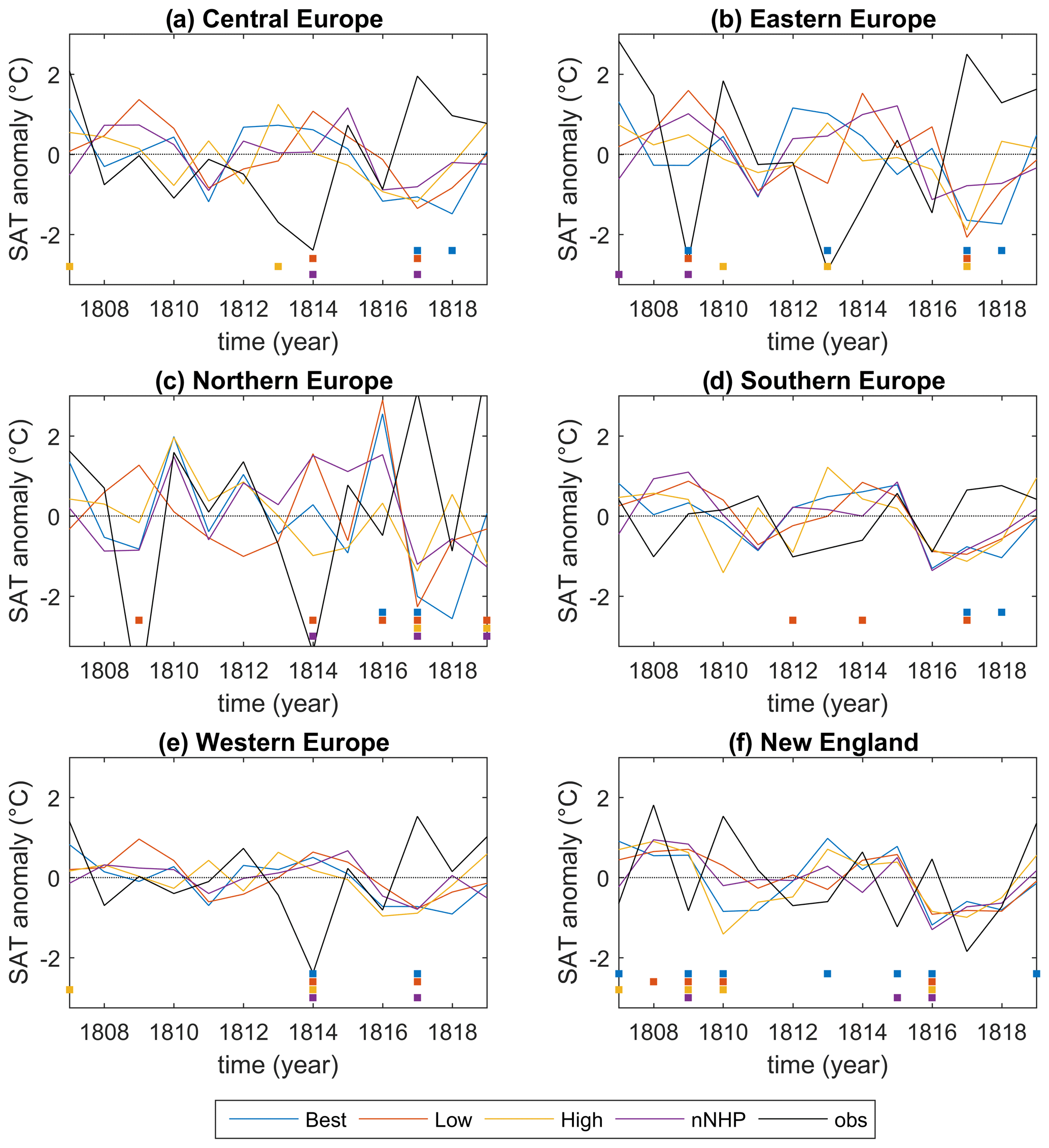
Figure 13Same as Fig. 12 but for seasonal mean near-surface NH winter temperature anomalies (∘C). The year corresponds to the month of February.
A comparison of simulated ensemble-mean and observed near-surface air temperature anomalies over different European regions and New England is shown for NH summer and winter in Figs. 12 and 13, respectively, as well as for the individual ensemble members, which show a variability comparable to the observations in the Supplement (Figs. S7–S14). Note that these figures neither account for the error in the observations nor the error (difference between a station and an areal average). For NH summer, the station data reflect the findings from the spatial comparison with the tree-ring records (Fig. 10); i.e., most European station records indicate some cooling in summer 1810 (Fig. 12a–e), while the New England data show no evidence of cooling in this year (Fig. 12f). Further, all of the stations show cooling in either 1812 or 1813, with many showing consecutive cold summers until the Tambora eruption of 1815. In boreal summer 1810, the nNHP and Low simulations and station data are inconsistent over northern Europe (Fig. 13c), where the observed cooling is larger than in the simulations, whereas for the High and Best experiments the station data lie within the ensemble range. Surface air temperature over western and central Europe seems to be mostly unaffected by the 1809 eruption all model experiments and in the station data (Fig. 12a, e). The simulated post-volcanic cooling in summer 1810 is consistent with the station data over southern and eastern Europe in the model experiments with symmetric volcanic forcing (Best, High, Low), but nNHP shows slightly warm anomalies for summer 1810 (Fig. 12d, b). In contrast, nNHP is the only experiment which shows a similar trend as the New England stations, whereas the other experiments show stronger cooling there in 1810. Observed cooling after the Mt. Tambora eruption is matched quite well by the model, except for central Europe and western Europe where the observed anomalies in 1816 are larger. Excellent agreement between model simulations and station data is found for the “year without summer” for New England. An interesting feature is the observed warming peak of 2 ∘C in summer 1811 over central Europe, which is also found in one realization of the Best experiment (Fig. S7), suggesting the influence of internal variability. For NH winter, both model and station data show higher variability than in NH summer (Fig. 13). Simulated and observed NH winter temperature anomalies agree quite well in the first three winters after the 1809 eruption. The only exception is New England (Fig. 13f) where, similar to NH summer (Fig. 12f), less agreement is found between the station data and the four experiments. The strong cooling signal of more than −2 ∘C which is found at northern, western, and central European stations in winter 1813/1814 is not reproduced by the model simulations. All experiments except the Low experiment produce positive post-volcanic winter temperature anomalies over northern Europe, with a warming signal in the first winter (1809/1810) after the 1809 eruption, consistent with the station data.
Significant surface cooling is found after the unidentified 1809 eruption in instrumental observations, proxy records, and simulations, but the cooling is strongly spatially heterogeneous and is variable across the different data sources, especially across the NH extratropics.
Observed and simulated cooling in the tropics is considerable, with anomalies likely exceeding 0.5 ∘C. In general, the MPI-ESM simulations show stronger cooling over the tropical oceans than the reconstructed and observed temperatures (Fig. 6). Over the tropical Indian Ocean, the simulated SST anomalies between 1809 and 1820 for the Low, Best, and nNHP experiments agree quite well with the marine ship measurements (Fig. 8). Furthermore, the ensemble-mean cooling in the Low experiment is close to the reconstruction of D'Arrigo et al. (2006) over the tropical Indo-Pacific in 1809, although the reconstruction does not pick up the 1816 cooling expressed by all experiments (Fig. 6c). An even smaller SST variability range is also found for the Indian and the western Pacific SST reconstructions when compared to the models (Fig. 7). Uncertainties related to the proxy measurements likely explain some of the mismatch, as they depend on several factors such as mixed sea surface temperature and salinity influences on the δ18O measurements in coral archives as well as seasonal changes in the growth rate and other biological factors. The limited number of proxy records, which are not equally distributed in time and space, is also undoubtedly a relevant factor. Focusing on the tropical region, the comparison between simulations suggests that the most probable forcing would be somewhere between Low, nNHP, and Best.
Simulated ensemble-mean NH extratropical summer temperature anomalies are mostly within the reconstructed range for all forcing scenarios, but the agreement is strongly dependent on the choice of the year, spatial coverage, and the individual forcing scenarios and reconstruction used. Ensemble-mean temperature differences between the different MPI-ESM experiments and the individual reconstructions could be of the order of the forced signal (Fig. 9). The NH mean summer temperature response to the 1809 eruption is smaller in tree-ring reconstructions than in the simulations (except for nNHP), consistent with previous comparisons of tree-ring reconstructions with climate models. Schneider et al. (2017), for example, compared tree-ring reconstructions with PMIP3 last millennium simulations from different models including the MPI-ESM. They also found that on average most model simulations feature a more pronounced volcanic signal than proxy reconstructions. The spread of simulated NH temperature arising from uncertainties in the volcanic forcing estimate (VSSI) for the 1809 eruption is generally comparable to the spread in the NH tree-ring-based temperature reconstructions. It is therefore not possible to use one proxy result to strongly constrain the other, as we might if one distribution was much smaller than the other or if the overlap between the two was small. On the other hand, the disagreement between observed and simulated tropical temperatures in the High ensemble would suggest that VSSI estimates on the upper end of our estimated range are not likely, and qualitatively we might estimate that the most likely VSSI emissions for 1809 are between around 12 and 19 Tg S.
Instrumental records in Europe fit well with simulated temperatures using all forcing scenarios for both winter and summer seasons (Figs. 12, 13). In boreal winter, observations from most stations (except New England and eastern Europe) lie within the ensemble range of all four experiments within the first two post-volcanic winters. Internal variability in NH winter is high and can overwhelm volcanic forcing uncertainties, as pointed out by Zanchettin et al. (2019) for the first winter after the Mt. Tambora eruption. The spread of continental winter responses generated by the initial conditions for the unidentified 1809 eruption is expected to be larger than for the Mt. Tambora eruption due to the lower signal-to-noise ratio. Ultimately, comparison with early instrumental data must be made cautiously. Although regular meteorological measurements have been performed across Europe since the 17th and 18th centuries (Brönnimann et al., 2019b), continuous temperature measurements in the 1810s are rare due to the Napoleonic wars and there is a significant lack of regular temperature time series from other parts of the world for this period.
Spatial correlations over the NH between the simulations and the N-TREND (S) temperature reconstruction for NH summer 1810 are overall low. None of the anomalous patterns produced by the MPI-ESM, either under unperturbed conditions or volcanic forcing scenarios, reproduce the amplitude and structure of the reconstructed hemispheric temperature anomaly pattern particularly well in summer 1810, suggesting that the mismatch is most likely not attributable to the volcanic forcing. This possibly stems from the heterogeneous reconstructed anomalies that lack a clear spatial structure and provide a “noisy” target to the simulations. The quite unusual temperature pattern in N-TREND (S), with cold temperatures over Europe and Alaska and warm temperatures over eastern North America and northern Siberia, could be a potential cause of this. This heterogeneous spatial pattern in the tree-ring data is also reflected in the dampened cooling seen in the NH mean composite reconstructions (Fig. 9). Station observations seem to support this anomaly pattern by showing cooling only over northern and eastern Europe. Surface temperature reconstructions from an almost independent MXD network (Briffa et al., 2002) also indicate positive temperature anomalies over eastern Canada, north of 55∘ N, and east of 95∘ W but also regional cooling. Briffa et al. (2002) used MXD data only, which capture the short-time cooling after volcanic eruptions more reliably than RW-based reconstructions that are influenced by biological persistence (e.g., Anchukaitis et al., 2012; Esper et al., 2015; Lücke et al., 2019). In N-TREND (S) a combination of MXD, RW, and BI records are used and the prediction skill is spatially very variable, particularly over North America (Anchukaitis et al., 2017). The distinct east–west dipole pattern in the reconstruction could therefore be partly caused by a data quality issue as is certainly the case for central Asia, which is driven predominantly by tree-ring-width data. One possibility is that 1810 was a dynamically unusual but not unlikely year (Fig. 11) in terms of NH atmospheric circulation that led to warming over eastern North America which is not reflected in the simulated ensemble mean. While a few individual simulations produced a dipole temperature anomaly pattern over North America similar to that of the N-TREND (S) reconstruction when forced with volcanic aerosol, many other simulations did not, and the ensemble-mean correlation was close to zero for all forced ensembles. We can only conclude that in these simulations, the volcanic aerosol forcing did not lead to or increase the likelihood of the dipole North American pattern.
Overall, our model–data intercomparison suggests the middle to low range of the sulfate estimates for the unidentified 1809 eruption as the most realistic. However, the range of uncertainty is large, as observed and reconstructed data are sparse and cover a wide post-volcanic temperature anomaly range. Uncertainties in volcanic forcing are often discussed as one of the main causes of the discrepancy between simulated and reconstructed temperature response due to biases in magnitude and structure (e.g., Timmreck et al., 2009; Yang et al., 2019; Zhu et al., 2020). As discussed above, the spread of the different forcing ensembles is in the same range as the different tree-ring reconstructions; hence, it is difficult to reduce the forcing estimates. Nevertheless, our work does suggest that the response of large-scale NH climate indexes (Fig. S1) is sensitive not only to the magnitude of the volcanic forcing, but also its meridional structure, with, e.g., significant differences in the summer North Pacific Index (NPI) response for the Best and nNHP ensembles. This would support the idea that the structure of forcing is important in influencing circulation changes (e.g., Toohey et al., 2019). An asymmetric volcanic forcing scenario with less or no NH extratropical forcing, as in nNHP, provides one way in which tropical temperatures could respond strongly to a tropical eruption, while the NH temperature response could be more muted and prolonged, as suggested by some tree-ring reconstructions for 1809. This scenario, however, is at odds with the ice-core records, which show comparable deposition to Antarctica and Greenland, suggesting a global aerosol spread. Without a viable explanation for a mismatch between ice-core records and hemispheric radiative forcing, extreme hemispheric asymmetry (as in the nNHP scenario) must be concluded to be an unlikely reason for the muted NH mean temperature response to the 1809 eruption.
A factor which might have an influence on the mismatch between model results and proxy data is the season of the eruption, which has an impact on the climate response to volcanic eruptions (e.g., Stevenson et al., 2017; Predybaylo et al., 2020). We have not discussed this uncertainty for the 1809 eruption here as we chose January 1809 as the starting date following most studies that suggest that the eruption probably happened in boreal winter months across 1808 and 1809. Nevertheless, the timing of the eruption remains uncertain. Chenoweth (2001), for example, dated the 1809 eruption back to March–June 1808 based on a sudden cooling in Malaysian land surface temperature data and a peak cooling of marine air temperature in 1809. Taking the eruption's season into account may be important to fully characterize the range of climate responses compatible with the 1809 eruption and should be addressed in further studies.
One final caveat to our simulation–reconstruction comparison stems from the idealized nature of our experiments: our simulations are branched from a multi-centennial pre-industrial control run and use only volcanic aerosol forcing; they are not transient simulations with realistic full forcing (also including variations in solar and land-use forcing, etc.). Neglecting the reduced solar irradiance in the early 19th century could, for example, be one of the reasons why our model simulations do not show the slight cooling trend in summer surface temperature between 1810 and 1815 indicated by the NH tree-ring data. While this more idealized experimental setup has the advantage of better isolating the influence of volcanic forcing strength and structure alone, it complicates the comparison with observations and proxy reconstructions. Early 19th century ensemble simulations starting from a climate state with a more realistic past natural forcing, as planned for the CMIP6 VolMIP/PMIP “volc-cluster-mill”experiments (Zanchettin et al., 2016; Jungclaus et al., 2017), will allow for a more direct comparison with early instrumental data and paleoclimate reconstructions. Furthermore, they will also help to disentangle the processes which are specific to the MPI-ESM and which need discussion in a broader context.
We used the MPI Earth system model to study the climatic impacts of the unidentified 1809 eruption, the sixth-largest volcanic eruption of the last millennium. Our aim was to address the question of whether or not the short-term climate response to the 1809 eruption noted in observations and proxy-based climate reconstructions is compatible with a range of volcanic forcing estimates constructed based on estimated uncertainties in volcanic stratospheric injection from ice-core records. We demonstrated that the model simulations of the climate impacts of the 1809 eruption show generally good agreement with many of the available large-scale temperature reconstructions and early instrumental records. Assuming the model climate sensitivity is correct, this result implies that the eVolv2k VSSI estimate for the 1809 eruption is accurate within its reported uncertainty. Model–data intercomparison of tropical temperature anomalies, wherein the impact of direct radiative forcing is highlighted, suggests that the most likely forcing is somewhere between the Low and the Best scenarios, with an estimated sulfur emission between 12 and 19 Tg S. However, the limited data availability for this time period for the tropical region poses a caveat to this conclusion. Simulated NH average summer temperature anomalies are for all forcing scenarios within the observational and reconstructed range. The long-lasting cooling trend detected in observed and reconstructed NH average summer temperatures between 1810 and 1815, i.e., until the Mt. Tambora eruption, is not detected in the model simulations, except partly in nNHP. The reason for such a cooling trend thus remains unclear and needs to be further explored. The spatial correlation between simulated and reconstructed near-surface air temperatures over the NH in summer 1810 is low. Tree-ring-based gridded reconstructions of NH extratropical summer SAT show a highly heterogeneous anomaly pattern in 1810 with extensive regions of cold and warm anomalies, an east–west warm–cold dipole over North America, and variable temperature anomalies over Asia, which leads to a dampened NH average cooling for this year (Fig. 10). The pattern over North America is consistent with the limited available station observations from New England, which are represented by an almost independent MXD-based summer temperature reconstruction (Briffa et al., 2002), and is reproduced by some forced simulations and years from the control run, suggesting it is a plausible result of natural variability. In contrast, the reconstructed temperature pattern over Asia is not produced by any model simulation whether forced or control. Possible explanations for this model–data disagreement include deficiencies and uncertainties regarding both tools. In particular, the dendrochronological network remains weakly constrained over the central Asian region, especially with respect to available MXD or density-like parameters, and instrumental observations are sparse, especially prior to the 1950s, making calibration and validation difficult (Cook et al., 2013). Anchukaitis et al. (2017) clearly detailed poor reconstruction validation for many regions across North America as well as northeastern and central Asia. These regions must be targeted in ongoing proxy network development to update and develop new MXD or density-like parameter datasets which are proven to be superior proxies for volcanically forced summer cooling (e.g., Anchukaitis et al., 2012; D'Arrigo et al., 2013; Esper et al., 2015; Lücke et al., 2019). Concerning the simulations, beyond model deficiencies that may bias the response, our study demonstrates that choices regarding both volcanic forcing strength and spatial structure can similarly affect reconstruction–simulation comparisons. Specifically, it was shown that for the muted response to the 1809 eruption in the NH extratropics, agreement between reconstructions and simulations improves by weakening the magnitude of the eruption and, alternatively, by preventing the volcanic aerosol from spreading over the Northern Hemisphere. The forcing estimate of 1809, which is based on ice-core data, can only be improved by modeling experiments to narrow down the uncertainty range. This will be facilitated if further information on location and eruption season is identified. Recent advances in ice-core analysis can help to identify the source volcano of large historic eruptions by combining proximal tephra fallout with the geochemical analysis of ash shards in ice cores as done, for example, for the 1257 Samalas eruption (Lavigne et al., 2013), the Changbaishan eruption in 946 (Oppenheimer et al., 2017), the 431 CE Tierra Blanca Joven eruption of Ilopango (Smith et al., 2020), and the 1477 CE eruption of the Icelandic Veiðivötn–Bárðarbunga volcanic system (Abbott et al., 2021, this issue).
Finally, it is clear that improving temperature reconstruction accuracy by adding additional tree-ring density records in poorly replicated regions, also including the Southern Hemisphere, is needed. In summary, analysis of multiple climate records shows that the eruption of 1809 was certainly a “cold case” in the sense that it produced large-scale cooling, and that cooling is consistent with the range of sulfur emission and radiative forcing estimates deduced from ice-core records. In terms of attributing the eruption to a source volcano or explaining the spatially heterogeneous and temporally delayed cooling in the NH suggested by tree-ring networks, the investigation remains open.
Table A1Temperature observations from land stations used in this study; n is the number of available values in the 1806–1820 period. Sources are as follows. Dove: digitized from the collection of Friedrich Wilhelm Dove (Dove, 1838, 1839, 1842, 1845), NOAA: digitized from images held at the NOAA archive, DWD: German Weather Service, GHCN: Global Historical Climatology Network (Lawrimore et al., 2011), ISTI: International Surface Temperature Initiative (Rennie et al., 2014).
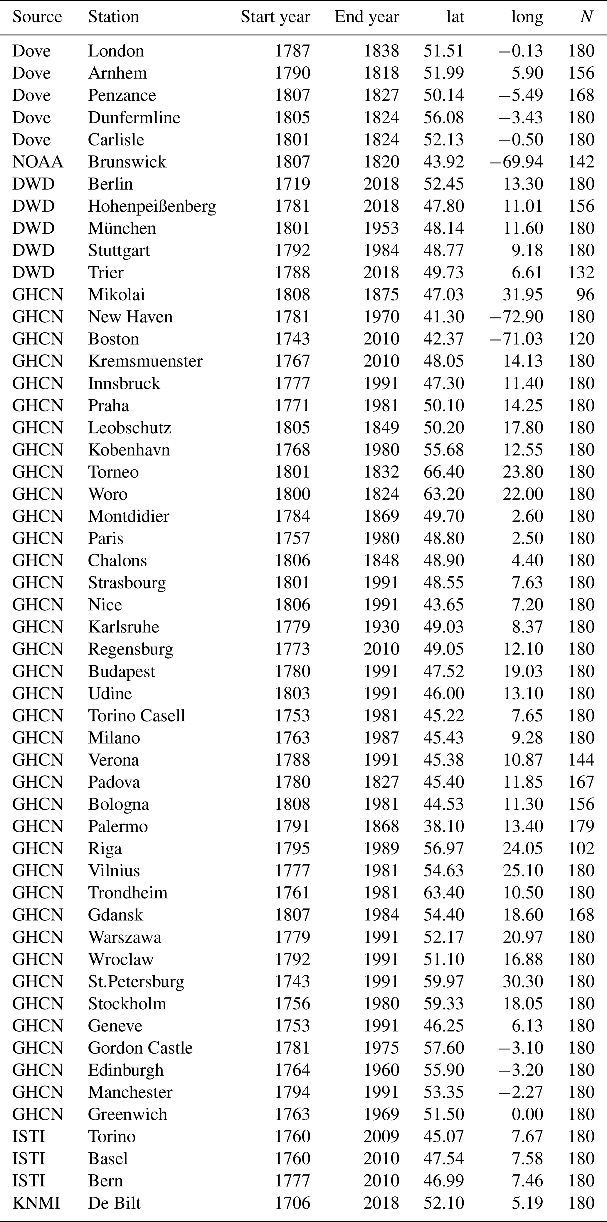
Table A2Overview of the different stations which are used in the compilation of the regional and seasonal station mean.
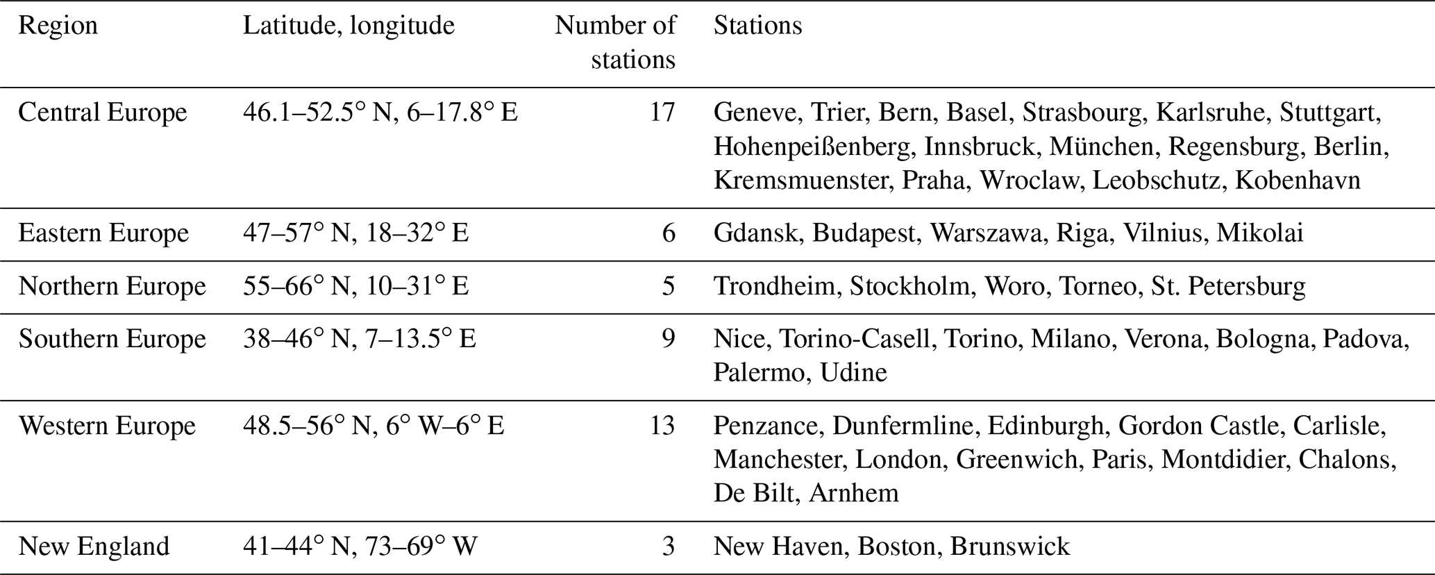
Primary data and scripts used in the analysis and other supplementary information that may be useful in reproducing this work are archived by the Max Planck Institute for Meteorology under http://hdl.handle.net/21.11116/0000-0008-B349-C (Timmreck, 2021). The proxy records analyzed in the paper are available in the published literature cited in the references.
The supplement related to this article is available online at: https://doi.org/10.5194/cp-17-1455-2021-supplement.
CT, MT, and DZ designed the study, analyzed the results, and wrote the paper. CT performed the simulations and coordinated the writing process. SB and RW provided data and contributed to the discussion and the writing process. EL compiled a new set of station data.
The authors declare that they have no conflict of interest.
Publisher's note: Copernicus Publications remains neutral with regard to jurisdictional claims in published maps and institutional affiliations.
This article is part of the special issue “Interdisciplinary studies of volcanic impacts on climate and society”. It is not associated with a conference.
The authors thank Stephan Lorenz, who gave valuable comments on an earlier version of the paper. This work used resources of the Deutsches Klimarechenzentrum (DKRZ) granted by its Scientific Steering Committee (WLA) under project ID bb1093. This work benefited from the participation of the authors in the Volcanic Impacts on Climate and Society (VICS) working group of the Past Global Changes (PAGES) project. Claudia Timmreck acknowledges support from the Deutsche Forschungsgemeinschaft Research Unit VolImpact (FOR2820, grant no. 398006378). Stefan Brönnimann acknowledges funding from the Swiss National Science Foundation project WeaR (grant no. 188701) and the European Commission through H2020 (ERC Grant, PALAEO-RA, grant no. 787574).
This research has been supported by the Deutsche Forschungsgemeinschaft Research Unit VolImpact (FOR2820, grant no. 398006378)
within the project VolClim, the European Commission, the European Research Council (PALAEO-RA (grant no. 787574)), and the Schweizerischer Nationalfonds zur Förderung der Wissenschaftlichen Forschung (WeaR; grant no. 188701).
The article processing charges for this open-access publication were covered by the Max Planck Society.
This paper was edited by Michael Sigl and reviewed by Oliver Bothe and one anonymous referee.
Abbott, P. M., Plunkett, G., Corona, C., Chellman, N. J., McConnell, J. R., Pilcher, J. R., Stoffel, M., and Sigl, M.: Cryptotephra from the Icelandic Veiðivötn 1477 CE eruption in a Greenland ice core: confirming the dating of volcanic events in the 1450s CE and assessing the eruption's climatic impact, Clim. Past, 17, 565–585, https://doi.org/10.5194/cp-17-565-2021, 2021. a
Anchukaitis, K. J., Breitenmoser, P., Briffa, K. R., Buchwal, A., Büntgen, U., Cook, E. R., D'Arrigo, R. D., Esper, J., Evans, M. N., Frank, D., Grudd, H., Gunnarson, B. E., Hughes, M. K., Kirdyanov, A. V., Körner, C., Krusic, P. J., Luckman, B., Melvin, T. M., Salzer, M. W., Shashkin, A. V., Timmreck, C., Vaganov, E. A., and Wilson, R. J. S.: Tree rings and volcanic cooling, Nat. Geosci., 5, 836–837, 2012. a, b, c
Anchukaitis, K. J., Wilson, R., Briffa, K. R., Büntgen, U., Cook, E. R., D’Arrigo, R., Davi, N., Esper, J., Frank, D.,Gunnarson, B. E., Hegerl, G., Helama, S., Klesse, S., Krusic, P. J., Linderholm, H. W., Myglan, V., Osborn, T. J., Zhang, P., Rydval, M., Schneider, L., Schurer, A., Wiles, G., and Zorita, E.: Last millennium Northern Hemisphere summer temperatures from tree rings: Part II, spatially resolved reconstructions, Quaternary Sci. Rev., 163, 1–22, 2017. a, b, c, d, e, f, g, h, i, j, k, l
Anet, J. G., Muthers, S., Rozanov, E. V., Raible, C. C., Stenke, A., Shapiro, A. I., Brönnimann, S., Arfeuille, F., Brugnara, Y., Beer, J., Steinhilber, F., Schmutz, W., and Peter, T.: Impact of solar versus volcanic activity variations on tropospheric temperatures and precipitation during the Dalton Minimum, Clim. Past, 10, 921–938, https://doi.org/10.5194/cp-10-921-2014, 2014. a
Briffa, K. R., Jones, P., and Schweingruber, F.: Tree-ring density reconstructions of summer temperature patterns across western North America since 1600, J. Climate, 5, 735–754, 1992. a, b
Briffa, K. R., Jones, P., and Schweingruber, F.: Summer temperatures across northern North America: Regional reconstructions from 1760 using tree-ring densities, J. Geophys. Res.-Atmos., 99, 25835–25844, 1994. a
Briffa, K. R., Schweingruber, F. H., Jones, P., Osborn, T., Shiyatov, S., and Vaganov, E.: Reduced sensitivity of recent tree-growth to temperature at high northern latitudes, Nature, 391, 678–682, 1998. a
Briffa, K. R., Osborn, T. J., Schweingruber, F. H., Jones, P. D., Shiyatov, S. G., and Vaganov, E. A.: Tree-ring width and density data around the Northern Hemisphere: Part 2, spatio-temporal variability and associated climate patterns, Holocene, 12, 759–789, 2002. a, b, c
Brohan, P., Allan, R., Freeman, E., Wheeler, D., Wilkinson, C., and Williamson, F.: Constraining the temperature history of the past millennium using early instrumental observations, Clim. Past, 8, 1551–1563, https://doi.org/10.5194/cp-8-1551-2012, 2012. a, b, c, d, e, f, g, h
Brönnimann, S. and Krämer, D.: Tambora and the “Year Without a Summer” of 1816. A Perspective on Earth and Human Systems Science, Geographica Bernensia, Bern, Switzerland, vol. 90, 2016. a
Brönnimann, S., Franke, J., Nussbaumer, S. U., Zumbühl, H. J., Steiner, D., Trachsel, M., Hegerl, G. C., Schurer, A., Worni, M., Malik, A., Flückiger, J., and Raible, C. C.: Last phase of the Little Ice Age forced by volcanic eruptions, Nat. Geosci., 12, 650–656, 2019a. a, b
Brönnimann, S., Allan, R., Ashcroft, L., Baer, S., Barriendos, M., Brázdil, R., Brugnara, Y., Brunet, M., Brunetti, M., Chimani, B., Cornes, R., Domínguez-Castro, F., Filipiak, J., Founda, D., Herrera, R. G., Gergis, J., Grab, S., Hannak, L., Huhtamaa, H., Jacobsen, K. S., Jones, P., Jourdain, S., Kiss, A., Lin, K. E., Lorrey, A., Lundstad, E., Luterbacher, J., Mauelshagen, F., Maugeri, M., Maughan, N., Moberg, A., Neukom, R., Nicholson, S., Noone, S., Nordli, O., Ólafsdóttir, K. B., Pearce, P. R., Pfister, L., Pribyl, K., Przybylak, R., Pudmenzky, C., Rasol, D., Reichenbach, D., Řezníčková, L., Rodrigo, F. S., Rohr, C., Skrynyk, O., Slonosky, V., Thorne, P., Valente, M. A., Vaquero, J. M., Westcottt, N. E., Williamson, F., and Wyszyński, P.: Unlocking pre-1850 instrumental meteorological records: A global inventory, B. Am. Meteorol. Soc., 100, ES389–ES413, 2019b. a, b
Chenoweth, M.: Two major volcanic cooling episodes derived from global marine air temperature, AD 1807–1827, Geophys. Res. Lett., 28, 2963–2966, 2001. a, b, c
Clyne, M., Lamarque, J.-F., Mills, M. J., Khodri, M., Ball, W., Bekki, S., Dhomse, S. S., Lebas, N., Mann, G., Marshall, L., Niemeier, U., Poulain, V., Robock, A., Rozanov, E., Schmidt, A., Stenke, A., Sukhodolov, T., Timmreck, C., Toohey, M., Tummon, F., Zanchettin, D., Zhu, Y., and Toon, O. B.: Model physics and chemistry causing intermodel disagreement within the VolMIP-Tambora Interactive Stratospheric Aerosol ensemble, Atmos. Chem. Phys., 21, 3317–3343, https://doi.org/10.5194/acp-21-3317-2021, 2021. a
Cole-Dai, J.: Volcanoes and climate, Wiley Interdisciplinary Reviews: Climate Change, 1, 824–839, 2010. a, b
Cole-Dai, J., Ferris, D., Lanciki, A., Savarino, J., Baroni, M., and Thiemens, M. H.: Cold decade (AD 1810–1819) caused by Tambora (1815) and another (1809) stratospheric volcanic eruption, Geophys. Res. Lett., 36, L22703, https://doi.org/10.1029/2009GL040882, 2009. a, b
Cook, E. R., Briffa, K. R., and Jones, P. D.: Spatial regression methods in dendroclimatology: a review and comparison of two techniques, Int. J. Climatol., 14, 379–402, 1994. a
Cook, E. R., Krusic, P. J., Anchukaitis, K. J., Buckley, B. M., Nakatsuka, T., and Sano, M.: Tree-ring reconstructed summer temperature anomalies for temperate East Asia since 800 CE, Clim. Dynam., 41, 2957–2972, 2013. a
Crowley, T. J. and Unterman, M. B.: Technical details concerning development of a 1200 yr proxy index for global volcanism, Earth Syst. Sci. Data, 5, 187–197, https://doi.org/10.5194/essd-5-187-2013, 2013. a
Dai, J., Mosley-Thompson, E., and Thompson, L. G.: Ice core evidence for an explosive tropical volcanic eruption 6 years preceding Tambora, J. Geophys. Res.-Atmos., 96, 17361–17366, 1991. a
DallaSanta, K., Gerber, E. P., and Toohey, M.: The circulation response to volcanic eruptions: The key roles of stratospheric warming and eddy interactions, J. Climate, 32, 1101–1120, 2019. a
D'Arrigo, R., Wilson, R., Palmer, J., Krusic, P., Curtis, A., Sakulich, J., Bijaksana, S., Zulaikah, S., Ngkoimani, L. O., and Tudhope, A.: The reconstructed Indonesian warm pool sea surface temperatures from tree rings and corals: Linkages to Asian monsoon drought and El Nino–Southern Oscillation, Paleoceanography, 21, PA3005, https://doi.org/10.1029/2005pa001256, 2006. a, b, c, d, e, f
D'Arrigo, R., Wilson, R., and Tudhope, A.: The impact of volcanic forcing on tropical temperatures during the past four centuries, Nat. Geosci., 2, 51–56, 2009. a, b, c, d, e, f, g
D'Arrigo, R., Wilson, R., and Anchukaitis, K. J.: Volcanic cooling signal in tree ring temperature records for the past millennium, J. Geophys. Res.-Atmos., 118, 9000–9010, 2013. a, b
Davi, N. K., Jacoby, G. C., and Wiles, G. C.: Boreal temperature variability inferred from maximum latewood density and tree-ring width data, Wrangell Mountain region, Alaska, Quaternary Res., 60, 252–262, 2003. a
Dove, H. W.: Über die nicht periodischen Änderungen der Temperaturvertheilung auf der Oberfläche der Erde. 1. Teil, Reimer, Berlin, Germany, 1838. a, b
Dove, H. W.: Über die nicht periodischen Änderungen der Temperaturvertheilung auf der Oberfläche der Erde. 2. Teil, Reimer, Berlin, Germany, 1839. a, b
Dove, H. W.: Über die nicht periodischen Änderungen der Temperaturvertheilung auf der Oberfläche der Erde. 3. Teil, Reimer, Berlin, Germany, 1842. a, b
Dove, H. W.: Über die nicht periodischen Änderungen der Temperaturvertheilung auf der Oberfläche der Erde. 1 Teil, Reimer, Berlin, Germany, 1845. a, b
Esper, J., Schneider, L., Smerdon, J. E., Schöne, B. R., and Büntgen, U.: Signals and memory in tree-ring width and density data, Dendrochronologia, 35, 62–70, 2015. a, b, c
Eyring, V., Bony, S., Meehl, G. A., Senior, C. A., Stevens, B., Stouffer, R. J., and Taylor, K. E.: Overview of the Coupled Model Intercomparison Project Phase 6 (CMIP6) experimental design and organization, Geosci. Model Dev., 9, 1937–1958, https://doi.org/10.5194/gmd-9-1937-2016, 2016. a
Fischer, E. M., Luterbacher, J., Zorita, E., Tett, S., Casty, C., and Wanner, H.: European climate response to tropical volcanic eruptions over the last half millennium, Geophys. Res. Lett., 34, L05707, https://doi.org/10.1029/2006GL027992, 2007. a
Franke, J., Frank, D., Raible, C. C., Esper, J., and Brönnimann, S.: Spectral biases in tree-ring climate proxies, Nat. Clim. Change, 3, 360–364, 2013. a
Gao, C., Robock, A., and Ammann, C.: Volcanic forcing of climate over the past 1500 years: An improved ice core-based index for climate models, Journal of Geophys. Res.-Atmos., 113, D23111, https://doi.org/10.1029/2008JD010239, 2008. a
Gennaretti, F., Boucher, E., Nicault, A., Gea-Izquierdo, G., Arseneault, D., Berninger, F., Savard, M. M., Bégin, C., and Guiot, J.: Underestimation of the Tambora effects in North American taiga ecosystems, Environ. Res. Lett., 13, 034017, https://doi.org/10.1088/1748-9326/aaac0c, 2018. a
Giorgetta, M. A., Jungclaus, J., Reick, C. H., Legutke, S., Bader, J., Böttinger, M., Brovkin, V., Crueger, T., Esch, M., Fieg, K., Glushak, K., Gayler, V., Haak, H., Hollweg, H., Ilyina, T., Kinne, S., Kornblueh, L., Matei, D., Mauritsen, T., Mikolajewicz, U., Mueller, W., Notz, D., Pithan, F., Raddatz, T., Rast, S., Redler, R., Roeckner, E., Schmidt, H., Schnur, R., Segschneider, J., Six, K. D., Stockhause, M., Timmreck, C., Wegner, J., Widmann, H., Wieners, K., Claussen, M., Marotzke, J., and Stevens, B.: Climate and carbon cycle changes from 1850 to 2100 in MPI-ESM simulations for the Coupled Model Intercomparison Project phase 5, J. Adv. Model. Earth Syst., 5, 572–597, 2013. a
Guevara-Murua, A., Williams, C. A., Hendy, E. J., Rust, A. C., and Cashman, K. V.: Observations of a stratospheric aerosol veil from a tropical volcanic eruption in December 1808: is this the Unknown ∼ 1809 eruption?, Clim. Past, 10, 1707–1722, https://doi.org/10.5194/cp-10-1707-2014, 2014. a
Guillet, S., Corona, C., Stoffel, M., Khodri, M., Lavigne, F., Ortega, P., Eckert, N., Sielenou, P. D., Daux, V., Churakova (Sidorova), O. V., Davi, N., Edouard, J.-L., Zhang, Y., Luckman, B. H., Myglan, V. S., Guiot, J., Beniston, M., Masson-Delmotte, V., and Oppenheimer, C.: Climate response to the Samalas volcanic eruption in 1257 revealed by proxy records, Nat. Geosci., 10, 123–128, 2017. a, b, c, d
Hakim, G. J., Emile-Geay, J., Steig, E. J., Noone, D., Anderson, D. M., Tardif, R., Steiger, N., and Perkins, W. A.: The last millennium climate reanalysis project: Framework and first results, J. Geophys. Res.-Atmos., 121, 6745–6764, 2016. a
Hartl-Meier, C., Büntgen, U., Smerdon, J. E., Zorita, E., Krusic, P. J., Ljungqvist, F. C., Schneider, L., and Esper, J.: Temperature covariance in tree ring reconstructions and model simulations over the past millennium, Geophys. Res. Lett., 44, 9458–9469, 2017. a
Haywood, J. M., Jones, A., Bellouin, N., and Stephenson, D.: Asymmetric forcing from stratospheric aerosols impacts Sahelian rainfall, Nat. Clim. Change, 3, 660–665, https://doi.org/10.1038/NCLIMATE1857, 2013. a
Hegerl, G. C., Crowley, T. J., Baum, S. K., Kim, K.-Y., and Hyde, W. T.: Detection of volcanic, solar and greenhouse gas signals in paleo-reconstructions of Northern Hemispheric temperature, Geophys. Res. Lett., 30, 1242, https://doi.org/10.1029/2002GL016635, 2003. a
Ilyina, T., Six, K. D., Segschneider, J., Maier-Reimer, E., Li, H., and Núñez-Riboni, I.: Global ocean biogeochemistry model HAMOCC: Model architecture and performance as component of the MPI-Earth system model in different CMIP5 experimental realizations, J. Adv. Model. Earth Syst., 5, 287–315, 2013. a
Jungclaus, J., Fischer, N., Haak, H., Lohmann, K., Marotzke, J., Matei, D., Mikolajewicz, U., Notz, D., and Von Storch, J.: Characteristics of the ocean simulations in the Max Planck Institute Ocean Model (MPIOM) the ocean component of the MPI-Earth system model, J. Adv. Model. Earth Syst., 5, 422–446, 2013. a
Jungclaus, J. H., Lohmann, K., and Zanchettin, D.: Enhanced 20th-century heat transfer to the Arctic simulated in the context of climate variations over the last millennium, Clim. Past, 10, 2201–2213, https://doi.org/10.5194/cp-10-2201-2014, 2014. a
Jungclaus, J. H., Bard, E., Baroni, M., Braconnot, P., Cao, J., Chini, L. P., Egorova, T., Evans, M., González-Rouco, J. F., Goosse, H., Hurtt, G. C., Joos, F., Kaplan, J. O., Khodri, M., Klein Goldewijk, K., Krivova, N., LeGrande, A. N., Lorenz, S. J., Luterbacher, J., Man, W., Maycock, A. C., Meinshausen, M., Moberg, A., Muscheler, R., Nehrbass-Ahles, C., Otto-Bliesner, B. I., Phipps, S. J., Pongratz, J., Rozanov, E., Schmidt, G. A., Schmidt, H., Schmutz, W., Schurer, A., Shapiro, A. I., Sigl, M., Smerdon, J. E., Solanki, S. K., Timmreck, C., Toohey, M., Usoskin, I. G., Wagner, S., Wu, C.-J., Yeo, K. L., Zanchettin, D., Zhang, Q., and Zorita, E.: The PMIP4 contribution to CMIP6 – Part 3: The last millennium, scientific objective, and experimental design for the PMIP4 past1000 simulations, Geosci. Model Dev., 10, 4005–4033, https://doi.org/10.5194/gmd-10-4005-2017, 2017. a, b
Kent, E. C., Rayner, N. A., Berry, D. I., Saunby, M., Moat, B. I., Kennedy, J. J., and Parker, D. E.: Global analysis of night marine air temperature and its uncertainty since 1880: The HadNMAT2 data set, J. Geophys. Res.-Atmos., 118, 1281–1298, 2013. a
Khodri, M., Izumo, T., Vialard, J., Janicot, S., Cassou, C., Lengaigne, M., Mignot, J., Gastineau, G., Guilyardi, E., Lebas, N., Robock, A., and McPhaden, M. J.: Tropical explosive volcanic eruptions can trigger El Niño by cooling tropical Africa, Nat. Commun., 8, 1–13, 2017. a
Lavigne, F., Degeai, J.-P., Komorowski, J.-C., Guillet, S., Robert, V., Lahitte, P., Oppenheimer, C., Stoffel, M., Vidal, C. M., Pratomo, I., Wassmer, P., Hajdas, I., Hadmoko, D. S., and de Belizal, E.: Source of the great AD 1257 mystery eruption unveiled, Samalas volcano, Rinjani Volcanic Complex, Indonesia, P. Natl. Acad. Sci. USA, 110, 16742–16747, 2013. a
Lawrimore, J. H., Menne, M. J., Gleason, B. E., Williams, C. N., Wuertz, D. B., Vose, R. S., and Rennie, J.: An overview of the Global Historical Climatology Network monthly mean temperature data set, version 3, J. Geophys. Res.-Atmos., 116, D19121, https://doi.org/10.1029/2011JD016187, 2011. a, b
Li, J., Xie, S. P., Cook, E. R., Morales, M. S., Christie, D. A., Johnson, N. C., Chen, F., D'Arrigo, R., Fowler, A. M., Gou, X., and Fang, K.: El Niño modulations over the past seven centuries, Nat. Clim. Change, 3, 822–826, 2013. a
Lücke, L. J., Hegerl, G. C., Schurer, A. P., and Wilson, R.: Effects of memory biases on variability of temperature reconstructions, J. Climate, 32, 8713–8731, 2019. a, b, c, d
Marshall, L., Johnson, J. S., Mann, G. W., Lee, L., Dhomse, S. S., Regayre, L., Yoshioka, M., Carslaw, K. S., and Schmidt, A.: Exploring how eruption source parameters affect volcanic radiative forcing using statistical emulation, J. Geophys. Res.-Atmos., 124, 964–985, 2019. a
Marshall, L. R., Smith, C. J., Forster, P. M., Aubry, T. J., Andrews, T., and Schmidt, A.: Large variations in volcanic aerosol forcing efficiency due to eruption source parameters and rapid adjustments, Geophys. Res. Lett., 47, e2020GL090241, https://doi.org/10.1029/2020GL090241, 2020. a
Mauritsen, T., Bader, J., Becker, T., Behrens, J., Bittner, M., Brokopf, R., Brovkin, V., Claussen, M., Crueger, T., Esch, M., Fast, I., Fiedler, S., Fläschner, D., Gayler, V., Giorgetta, M., Goll, D. S., Haak, H., Hagemann, S., Hedemann, C., Hohenegger, C., Ilyina, T., Jahns, T., Jimenéz-de-la Cuesta, D., Jungclaus, J., Kleinen, T., Kloster, S., Kracher, D., Kinne, S., Kleberg, D., Lasslop, G., Kornblueh, L., Marotzke, J., Matei, D., Meraner, K Mikolajewicz, U., Modali, K., Möbis, B., Müller, W. A., Nabel, J. E. M. S., Nam, C. C. W., Notz, D., Nyawira, S.-S., Paulsen, H., Peters, K., Pincus, R., Pohlmann, H., Pongratz, J., Popp, M., Raddatz, T. J., Rast, S., Redler, R., Reick, C. H., Rohrschneider, T., Schemann, V., Schmidt, H., Schnur, R., Schulzweida, U., Six, K. D., Stein, L., Stemmler, I., Stevens, B., Storch, J.-S., Tian, F., Voigt, A., Vrese, P., Wieners, K.-H., Wilkenskjeld, S., Winkler, A., and Roeckner, E.: Developments in the MPI-M Earth System Model version 1.2 (MPI-ESM1.2) and its response to increasing CO2, J. Adv. Model. Earth Syst., 11, 998–1038, 2019. a, b
McGregor, S., Timmermann, A., and Timm, O.: A unified proxy for ENSO and PDO variability since 1650, Clim. Past, 6, 1–17, https://doi.org/10.5194/cp-6-1-2010, 2010. a
Moreno-Chamarro, E., Zanchettin, D., Lohmann, K., and Jungclaus, J. H.: An abrupt weakening of the subpolar gyre as trigger of Little Ice Age-type episodes, Clim. Dynam., 48, 727–744, 2017. a
Müller, W. A., Jungclaus, J. H., Mauritsen, T., Baehr, J., Bittner, M., Budich, R., Bunzel, F., Esch, M., Ghosh, R., Haak, H., Ilyina, T., Kleine, T., Kornblueh, L., Li, H., Modali, K., Notz, D., Pohlmann, H., Roeckner, E., Stemmler, I., Tian, F., and Marotzke, J.: A Higher-resolution Version of the Max Planck Institute Earth System Model (MPI-ESM1. 2-HR), J. Adv. Model. Earth Syst., 10, 1383–1413, 2018. a
Oppenheimer, C.: Climatic, environmental and human consequences of the largest known historic eruption: Tambora volcano (Indonesia) 1815, Prog. Phys. Geogr., 27, 230–259, 2003. a
Oppenheimer, C., Wacker, L., Xu, J., Diego Galván, J., Stoffel, M., Guillet, S., Corona, C., Sigl, M., Di Cosmo, N., Hajdas, I., Pan, B., Breuker, R., Schneider, L., Esper, J., Fei, J., Hammond, J. O. S., and Büntgen, U.: Multi-proxy dating the “Millennium Eruption” of Changbaishan to late 946 CE, Quaternary Sci. Rev., 158, 164–171, 2017. a
PAGES 2k Consortium: Consistent multi-decadal variability in global temperature reconstructions and simulations over the Common Era, Nat. Geosci., 12, 643, https://doi.org/10.1038/s41561-019-0400-0, 2019. a
Pausata, F. S., Zanchettin, D., Karamperidou, C., Caballero, R., and Battisti, D. S.: ITCZ shift and extratropical teleconnections drive ENSO response to volcanic eruptions, Sci. Adv., 6, eaaz5006, https://doi.org/10.1126/sciadv.aaz5006, 2020. a
Plummer, C. T., Curran, M. A. J., van Ommen, T. D., Rasmussen, S. O., Moy, A. D., Vance, T. R., Clausen, H. B., Vinther, B. M., and Mayewski, P. A.: An independently dated 2000-yr volcanic record from Law Dome, East Antarctica, including a new perspective on the dating of the 1450s CE eruption of Kuwae, Vanuatu, Clim. Past, 8, 1929–1940, https://doi.org/10.5194/cp-8-1929-2012, 2012. a
Predybaylo, E., Stenchikov, G., Wittenberg, A. T., and Osipov, S.: El Niño/Southern Oscillation response to low-latitude volcanic eruptions depends on ocean pre-conditions and eruption timing, Communications Earth & Environment, 1, 1–13, 2020. a
Raible, C. C., Brönnimann, S., Auchmann, R., Brohan, P., Frölicher, T. L., Graf, H.-F., Jones, P., Luterbacher, J., Muthers, S., Neukom, R., Robock, A., Self, S., Sudrajat, A., Timmreck, C., and Wegmann, M.: Tambora 1815 as a test case for high impact volcanic eruptions: Earth system effects, Wiley Interdisciplinary Reviews: Climate Change, 7, 569–589, 2016. a
Rao, M. P., Cook, B. I., Cook, E. R., D’Arrigo, R. D., Krusic, P. J., Anchukaitis, K. J., LeGrande, A. N., Buckley, B. M., Davi, N. K., Leland, C., and Griffin, K. L.: European and Mediterranean hydroclimate responses to tropical volcanic forcing over the last millennium, Geophys. Res. Lett., 44, 5104–5112, 2017. a
Reick, C. H., Raddatz, T., Brovkin, V., and Gayler, V.: Representation of natural and anthropogenic land cover change in MPI-ESM, J. Adv. Model. Earth Syst., 5, 459–482, https://doi.org/10.1002/jame.20022, 2013. a
Rennie, J., Lawrimore, J., Gleason, B., Thorne, P., Morice, C., Menne, M., Williams, C., Almeida, W. G., Christy, J., Flannery, M., Ishihara, M., Kamiguchi, K., Klein-Tank, A. M. G., Mhanda, A., Lister, D. H., Razuvaev, V., Renom, M., Rusticucci, M., Tandy, J., Worley, S. J., Venema, V., Angel, W., Brunet, M., Dattore, B., Diamond, H., Lazzara, M. A., Le Blancq, F., Luterbacher, J., Mächel, H., Revadekar, J., Vose, R. S., and Yin, X.: The international surface temperature initiative global land surface databank: Monthly temperature data release description and methods, Geosci. Data J., 1, 75–102, 2014. a, b
Robock, A.: Volcanic eruptions and climate, Rev. Geophys., 38, 191–219, 2000. a
Schneider, L., Smerdon, J. E., Büntgen, U., Wilson, R. J., Myglan, V. S., Kirdyanov, A. V., and Esper, J.: Revising midlatitude summer temperatures back to AD 600 based on a wood density network, Geophys. Res. Lett., 42, 4556–4562, 2015. a, b, c, d, e, f, g
Schneider, L., Smerdon, J. E., Pretis, F., Hartl-Meier, C., and Esper, J.: A new archive of large volcanic events over the past millennium derived from reconstructed summer temperatures, Environ. Res. Lett., 12, 094005, https://doi.org/10.1088/1748-9326/aa7a1b, 2017. a, b, c, d
Schurer, A. P., Hegerl, G. C., Luterbacher, J., Brönnimann, S., Cowan, T., Tett, S. F., Zanchettin, D., and Timmreck, C.: Disentangling the causes of the 1816 European year without a summer, Environ. Res. Lett., 14, 094019, https://doi.org/10.1088/1748-9326/ab3a10, 2019. a, b
Schweingruber, F., Briffa, K., and Jones, P.: Yearly maps of summer temperatures in Western Europe from AD 1750 to 1975 and Western North America from 1600 to 1982, Vegetatio, 92, 5–71, 1991. a
Shindell, D. T., Schmidt, G. A., Mann, M. E., and Faluvegi, G.: Dynamic winter climate response to large tropical volcanic eruptions since 1600, J. Geophys. Res.-Atmos., 109, D05104, https://doi.org/10.1029/2003JD004151, 2004. a
Sigl, M., McConnell, J. R., Layman, L., Maselli, O., McGwire, K., Pasteris, D., Dahl‐Jensen, D., Steffensen, J. P., Vinther, B., Edwards, R., and Mulvaney, R.: A new bipolar ice core record of volcanism from WAIS Divide and NEEM and implications for climate forcing of the last 2000 years, J. Geophys. Res.-Atmos., 118, 1151–1169, 2013. a
Sigl, M., Winstrup, M., McConnell, J. R., Welten, K. C., Plunkett, G., Ludlow, F., Büntgen, U., Caffee, M., Chellman, N., Dahl-Jensen, D., Fischer, H., Kipfstuhl, S., Kostick, C., Maselli, O. J., Mekhaldi, F., Mulvaney, R., Muscheler, R., Pasteris, D. R., Pilcher, J. R., Salzer, M., Schüpbach, S., Steffensen, J. P., Vinther, B. M., and Woodruff, T. E.: Timing and climate forcing of volcanic eruptions for the past 2500 years, Nature, 523, 543–549, 2015. a
Smith, V. C., Costa, A., Aguirre-Díaz, G., Pedrazzi, D., Scifo, A., Plunkett, G., Poret, M., Tournigand, P.-Y., Miles, D., Dee, M. W., McConnell, J. R., Sunyé-Puchol Dávila Harris, P., Sigl, M., Pilcher, J. R., Chellman, N., and Gutiérrez, E.: The magnitude and impact of the 431 CE Tierra Blanca Joven eruption of Ilopango, El Salvador, P. Natl. Acad. Sci. USA, 117, 26061–26068, 2020. a
Stevens, B., Giorgetta, M., Esch, M., Mauritsen, T., Crueger, T., Rast, S., Salzmann, M., Schmidt, H., Bader, J., Block, K., Brokopf, R., Fast, I., Kinne, S., Kornblueh, L., Lohmann, U., Pincus, R., Reichler, T., and Roeckner, E.: Atmospheric component of the MPI-M Earth system model: ECHAM6, J. Adv. Model. Earth Syst., 5, 146–172, 2013. a
Stevenson, S., Fasullo, J. T., Otto-Bliesner, B. L., Tomas, R. A., and Gao, C.: Role of eruption season in reconciling model and proxy responses to tropical volcanism, P. Natl. Acad. Sci. USA, 114, 1822–1826, 2017. a
Stoffel, M., Khodri, M., Corona, C., Guillet, S., Poulain, V., Bekki, S., Guiot, J., Luckman, B. H., Oppenheimer, C., Lebas, N., Beniston, M., and Masson-Delmotte, V.: Estimates of volcanic-induced cooling in the Northern Hemisphere over the past 1,500 years, Nat. Geosci., 8, 784–788, 2015. a
Tierney, J. E., Abram, N. J., Anchukaitis, K. J., Evans, M. N., Giry, C., Kilbourne, K. H., Saenger, C. P., Wu, H. C., and Zinke, J.: Tropical sea surface temperatures for the past four centuries reconstructed from coral archives, Paleoceanography, 30, 226–252, 2015. a, b, c
Timmreck, C.: Modeling the climatic effects of large explosive volcanic eruptions, Wiley Interdisciplinary Reviews: Climate Change, 3, 545–564, 2012. a
Timmreck, C.: Primary data for “The unidentified eruption of 1809: a climatic cold case”, Max Planck Institute for Meteorology, available at: http://hdl.handle.net/21.11116/0000-0008-B349-C, last access: 12 July 2021. a
Timmreck, C., Lorenz, S. J., Crowley, T. J., Kinne, S., Raddatz, T. J., Thomas, M. A., and Jungclaus, J. H.: Limited temperature response to the very large AD 1258 volcanic eruption, Geophys. Res. Lett., 36, L21708, https://doi.org/10.1029/2009GL040083, 2009. a
Toohey, M. and Sigl, M.: Volcanic stratospheric sulfur injections and aerosol optical depth from 500 BCE to 1900 CE, Earth Syst. Sci. Data, 9, 809–831, https://doi.org/10.5194/essd-9-809-2017, 2017. a, b, c, d, e
Toohey, M., Krüger, K., Niemeier, U., and Timmreck, C.: The influence of eruption season on the global aerosol evolution and radiative impact of tropical volcanic eruptions, Atmos. Chem. Phys., 11, 12351–12367, https://doi.org/10.5194/acp-11-12351-2011, 2011. a
Toohey, M., Stevens, B., Schmidt, H., and Timmreck, C.: Easy Volcanic Aerosol (EVA v1.0): an idealized forcing generator for climate simulations, Geosci. Model Dev., 9, 4049–4070, https://doi.org/10.5194/gmd-9-4049-2016, 2016. a, b, c
Toohey, M., Krüger, K., Schmidt, H., Timmreck, C., Sigl, M., Stoffel, M., and Wilson, R.: Disproportionately strong climate forcing from extratropical explosive volcanic eruptions, Nat. Geosci., 12, 100, https://doi.org/10.1038/s41561-018-0286-2, 2019. a, b
Wegmann, M., Brönnimann, S., Bhend, J., Franke, J., Folini, D., Wild, M., and Luterbacher, J.: Volcanic influence on European summer precipitation through monsoons: possible cause for “Years without Summer”, J. Climate, 27, 3683–3691, 2014. a
Wilson, R., Anchukaitis, K., Briffa, K., Büntgen, U., Cook, E., D'Arrigo, R., Davi, N., Esper, J., Frank, D., Gunnarson, B., Hegerl, G., Klesse, S., Krusic, P., Linderholm, H., Myglan, V., Peng, Z., Rydval, M., Schneider, L., Schurer, A., Wiles, G., and Zorita, E.: Last millennium northern hemisphere summer temperatures from tree rings: Part I: The long term context, Quaternary Sci. Rev., 134, 1–18, 2016. a, b, c, d, e, f, g, h, i, j, k
Wilson, R., Anchukaitis, K., Andreu-Hayles, L., Cook, E., D'Arrigo, R., Davi, N., Haberbauer, L., Krusic, P., Luckman, B., Morimoto, D., Oelkers, R., Wiles, G., and Wood, C.: Improved dendroclimatic calibration using blue intensity in the southern Yukon, Holocene, 29, 1817–1830, 2019. a
Winter, A., Zanchettin, D., Miller, T., Kushnir, Y., Black, D., Lohmann, G., Burnett, A., Haug, G. H., Estrella-Martínez, J., Breitenbach, S. F. M, Beaufort, L., Rubino, A., and Cheng, H.: Persistent drying in the tropics linked to natural forcing, Nat. Commun., 6, 1–8, 2015. a
Wunderlich, F. and Mitchell, D. M.: Revisiting the observed surface climate response to large volcanic eruptions, Atmos. Chem. Phys., 17, 485–499, https://doi.org/10.5194/acp-17-485-2017, 2017. a
Yang, W., Vecchi, G. A., Fueglistaler, S., Horowitz, L. W., Luet, D. J., Muñoz, Á. G., Paynter, D., and Underwood, S.: Climate Impacts From Large Volcanic Eruptions in a High-Resolution Climate Model: The Importance of Forcing Structure, Geophys. Res. Lett., 46, 7690–7699, 2019. a, b
Zanchettin, D., Bothe, O., Graf, H. F., Lorenz, S. J., Luterbacher, J., Timmreck, C., and Jungclaus, J. H.: Background conditions influence the decadal climate response to strong volcanic eruptions, J. Geophys. Res.-Atmos., 118, 4090–4106, 2013. a
Zanchettin, D., Bothe, O., Lehner, F., Ortega, P., Raible, C. C., and Swingedouw, D.: Reconciling reconstructed and simulated features of the winter Pacific/North American pattern in the early 19th century, Clim. Past, 11, 939–958, https://doi.org/10.5194/cp-11-939-2015, 2015. a
Zanchettin, D., Khodri, M., Timmreck, C., Toohey, M., Schmidt, A., Gerber, E. P., Hegerl, G., Robock, A., Pausata, F. S. R., Ball, W. T., Bauer, S. E., Bekki, S., Dhomse, S. S., LeGrande, A. N., Mann, G. W., Marshall, L., Mills, M., Marchand, M., Niemeier, U., Poulain, V., Rozanov, E., Rubino, A., Stenke, A., Tsigaridis, K., and Tummon, F.: The Model Intercomparison Project on the climatic response to Volcanic forcing (VolMIP): experimental design and forcing input data for CMIP6, Geosci. Model Dev., 9, 2701–2719, https://doi.org/10.5194/gmd-9-2701-2016, 2016. a, b
Zanchettin, D., Timmreck, C., Toohey, M., Jungclaus, J. H., Bittner, M., Lorenz, S. J., and Rubino, A.: Clarifying the relative role of forcing uncertainties and initial-condition unknowns in spreading the climate response to volcanic eruptions, Geophys. Res. Lett., 46, 1602–1611, 2019. a, b, c, d, e, f
Zhu, F., Emile-Geay, J., Hakim, G. J., King, J., and Anchukaitis, K. J.: Resolving the differences in the simulated and reconstructed temperature response to volcanism, Geophys. Res. Lett., 47, e2019GL086908, https://doi.org/10.1029/2019GL086908, 2020. a, b
- Abstract
- Introduction
- Methods and data
- The 1809 eruption in climatic observations and proxy records
- Results
- Discussion
- Conclusions
- Appendix A: Station data
- Code and data availability
- Author contributions
- Competing interests
- Disclaimer
- Special issue statement
- Acknowledgements
- Financial support
- Review statement
- References
- Supplement