Assessing the statistical uniqueness of the Younger Dryas: a robust multivariate analysis

During the last glacial period (ca. 120–11 kyr BP), dramatic temperature swings, known as Dansgaard–Oeschger (D–O) events, are clearly manifest in high-resolution oxygen isotope records from the Greenland Ice Sheet. Although variability in the Atlantic Meridional Overturning Circulation (AMOC) is often invoked, a unified explanation for what caused these “sawtooth-shaped” climate patterns has yet to be accepted. Of particular interest is the most recent D–O-shaped climate pattern that occurred from ∼ 14 600 to 11 500 years ago – the Bølling–Allerød (BA) warm interstadial and the subsequent Younger Dryas (YD) cold stadial. Unlike earlier D–O stadials, the YD is frequently considered a unique event, potentially resulting from a rerouting and/or flood of glacial meltwater into the North Atlantic or a meteorite impact. Yet, these mechanisms are less frequently considered as the cause of the earlier stadials. Using a robust multivariate outlier detection scheme – a novel approach for traditional paleoclimate research – we show that the pattern of climate change during the BA/YD is not statistically different from the other D–O events in the Greenland record and that it should not necessarily be considered unique when investigating the drivers of abrupt climate change. In so doing, our results present a novel statistical framework for paleoclimatic data analysis.

1 Introduction

First noted in 1985 by Willi Dansgaard as “violent oscillations” in Greenland's DYE-3 and Camp Century oxygen isotope (δ¹⁸O) records, Dansgaard–Oeschger (D–O) events are now well-known examples of abrupt climate change during the last glacial period (ca. 120–11 kyr BP) (see Fig. 1) (Dansgaard, 1985). These events are characterized by abrupt warmings of ∼8–16 ^∘C and a subsequent centennial- to millennial-length period of relative warmth (i.e., an interstadial), followed by a gradual, and sometimes abrupt, shift to cooler (stadial) conditions (Rasmussen et al., 2014). Since their discovery 3.5 decades ago, countless mechanisms have been proposed to explain D–O cycles (see Li and Born, 2019, for a review). Although most hypotheses invoke changes in ocean heat transport as a consequence of variations in the strength of the Atlantic Meridional Overturning Circulation (AMOC) (Broecker et al., 1985), the causes of such large and rapid changes in the overturning cell are not well understood (Lohmann and Ditlevsen, 2019). While variations in atmospheric circulation, sea ice extent, and ice shelf formation and collapse have all been hypothesized as triggers (Li and Born, 2019), a unifying theory has yet to emerge (Lohmann and Ditlevsen, 2018). Given that D–O events provide compelling evidence that the global climate can rapidly switch from one state to another, it is imperative that we determine the causes of this variability if we are to accurately predict future climate.

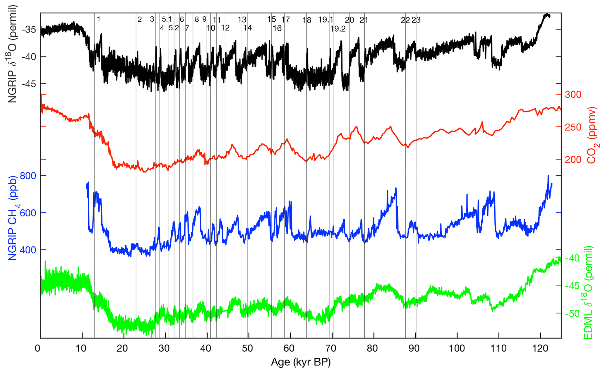
Figure 1 Full time series of all four records used. From top down: NGRIP δ¹⁸O (Rasmussen et al., 2014) compiled CO₂ from EDML, WAIS, Siple Dome, and TALDICE (Bereiter et al., 2015), NGRIP CH₄ (Baumgartner et al., 2014), and EDML δ¹⁸O (Barbante et al., 2006). Vertical lines indicate the 25 main interstadial-to-stadial transitions used in this study, which are labeled by number from Rasmussen et al. (2014).

In the original work of Dansgaard (Dansgaard, 1985), the most recent sawtooth-shaped interstadial–stadial sequence of climate change since 120 000 years ago, associated with the Bølling–Allerød warming and Younger Dryas stadial (abbreviated here to BA/YD) from ∼ 14 600 to 11 700 years BP, was labeled as D–O event 1 (Fig. 1). Since then, however, a growing body of geological evidence attributing the Younger Dryas cooling to a glacial outburst flood and/or a change in glacial meltwater drainage patterns to the ocean (Broecker et al., 1989; Clark et al., 2001; Keigwin et al., 2018) has sometimes led to this episode being treated as a unique event rather than as one of the D–O stadials (Li and Born, 2019). Evidence that the YD cooling might have also coincided with a meteorite impact capable of “blocking out” incoming solar radiation has helped bolster this notion (Firestone et al., 2007). In this paper, we use a multivariate outlier method to re-examine the extent to which the BA/YD should be considered “unique” in the context of the other D–O events. The motivation for this study derives from the remarkable similarities in shape (see further definition of shape below) between the BA/YD and other D–O events within the last 120 000 years, which leads us to question the uniqueness of the BA/YD in the Greenland record. Our approach is particularly novel for traditional paleoclimate research, and we suggest it may be useful in future studies with similar aims. It should also be noted that modeling studies suggest that forced and unforced AMOC variations have very similar signatures (Brown and Galbraith, 2016), so the outlier detection technique is not aimed to assess the qualities of D–O events as they result from specific triggers, but rather to provide a framework for situating the BA/YD within a broader context of many other D–O events, each of which may (or may not) have the same underlying trigger.

2 Methods

To study abrupt decadal to multidecadal changes in climate associated with each of the Dansgaard–Oeschger events, we examined published changes in oxygen isotope ratios (δ¹⁸O) and methane (CH₄) from the NGRIP Greenland ice cores (Rasmussen et al., 2014; Baumgartner et al., 2014) and δ¹⁸O and carbon dioxide (CO₂) changes from the EDML, WAIS, Siple Dome, and TALDICE ice cores recovered from Antarctica (Barbante et al., 2006; Bereiter et al., 2015) that span the last 120 000 years of Earth's climate history. Our NGRIP and EDML records both use the GICC05 age scale, and EDML was chosen because its spatial resolution and record length are comparable to the Greenland ice core records. Indeed, the snow accumulation at EDML is 2 to 3 times higher than at other deep drilling sites on the East Antarctic plateau, so higher-resolution atmosphere and climate records can be obtained for the last glacial period, making the EDML core especially suitable for studying decadal to millennial climate variations in Antarctica. Including EDML δ¹⁸O allows us to observe changes in NGRIP δ¹⁸O as distinct in location but similar in meaning. This allows us to make conclusions about how the BA/YD may not have been a unique event in Greenland, but perhaps was so in the southern Atlantic. In general, our choice of records is based on those with the highest spatial resolution and tradition in the field of paleoclimatology of using these to study climate variability during both D–O events and the BA/YD. The high temporal resolution of the ice cores during the last glacial period makes them ideal for use in our work. Both δ¹⁸O records (NGRIP and EDML) provide local approximations of climate, CH₄ is a globally integrated signal indicative of hydrology in wetland regions (Brook et al., 2000), and CO₂ shows a strong correlation with Antarctic temperature on millennial scales (Bauska et al., 2021).

For the purposes of our study, the timing of each Dansgaard–Oeschger event is taken from the ages published in the INTIMATE (INTegration of Ice-core, MArine and TErrestrial records) dataset in Table 2 of Rasmussen et al. (2014). We then develop a stratigraphy that emphasizes the large-scale Dansgaard–Oeschger variability as follows: firstly, all sub-interstadials in the INTIMATE record of Rasmussen et al. (2014) that are labeled by lowercase letters are very small, so we consider these to be part of the larger interstadial and not unique events. For example, while Greenland Interstadial 1 (i.e., the BA interstadial) is comprised of sub-events GI-1a through GI-1e, in our analysis this is simply treated as GI-1. A second set of sub-events in the INTIMATE dataset is also denoted by decimals in Rasmussen et al. (2014). For example, Dansgaard–Oeschger event 2 in the INTIMATE dataset is separated into two sub-events labeled GS 2.1/GI2.1 and GS 2.2/GI 2.2. Due to their generally high amplitude and tendency to span multi-centennial timescales, these sub-events must at least initially be considered as Dansgaard–Oeschger “candidates” and thus require a more rigorous procedure to be dealt with. Firstly, we consider cases when two sub-events occur in succession and define a duration-based algorithm to determine whether each one should be considered a separate Dansgaard–Oeschger event, both combined into one single event, or omitted from our analysis entirely. Figure 2 outlines this algorithmic consolidation process in the form of a flowchart using parameters x, y, and z.

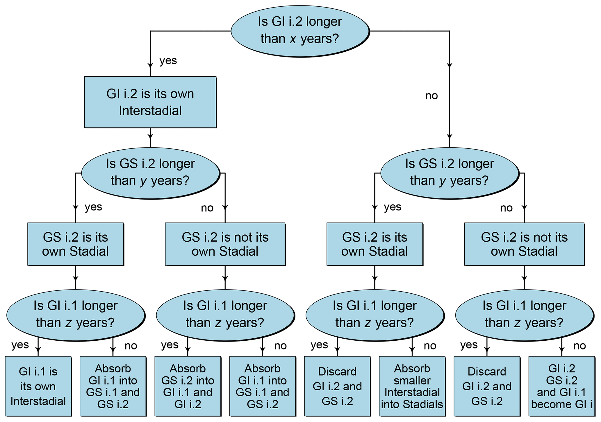
Figure 2 Decision tree for determining which warm–cold intervals split up by the INTIMATE stratigraphy can confidently be considered their own unique D–O events. Given the variety of climatic shifts present in the high-resolution INTIMATE NGRIP δ¹⁸O stratigraphy, it is necessary to form a rigorous criterion for choosing D–O events to analyze. Since the duration of each D–O event in the INTIMATE stratigraphy is directly tied to the confidence that it exhibits the true characteristics of a D–O interstadial (stadial) period, we employ the above duration-based scheme with flexible parameters $(x,y,z)$ in order to determine which D–O cycles to include in this analysis.

Of the eight Dansgaard–Oeschger events in this period containing two sub-events – namely numbers 2, 5, 15, 16, 17, 19, 21, and 23 – our main analysis leads to the selection of the stadials and interstadials found in Table 1. The selection of these events is based on using duration parameter choices: x=300 years, y=300 years, and z=200 years, which are at the shorter end of what has previously been accepted as the length of a stadial or interstadial (e.g., Rasmussen et al., 2014), but our results are not very sensitive to the chosen length. For example, columns 2–3 of Table 1 show that altering these parameters to $(x,y,z)=(\mathrm{90},\mathrm{100},\mathrm{140})$ or $(x,y,z)=(\mathrm{90},\mathrm{100},\mathrm{90})$ yields results that are 86 %–93 % similar.

Table 1 Three different stadial choice situations for different duration parameter choices in Fig. 2. The choice results in the first column ($(x,y,z)=(\mathrm{300},\mathrm{300},\mathrm{200})$) represent our preferred choices for statistical analysis. Note that basing the analysis on the stratigraphic choices represented in the second or third columns yields 86 %–93 % similarity in results.

Taking D–O event 2 as an example, we observe that GI2.2, GS2.2, and GI2.1 span 120, 200, and 120 years, respectively, and thus the algorithm in Fig. 2 leads to the combination of GI2.2, GS2.2, and GI2.1 into a single interstadial, since the sub-events are less than the parameter choices x=300, y=300, and z=200, respectively. In D–O event 5, however, GI5.2, GS5.2, and GI5.1 span 460, 1200, and 240 years, respectively, and thus under the same parameter choices, the interstadial–stadial choice algorithm in Fig. 2 dictates that each sub-event should be treated as its own stadial or interstadial. Note that our final results differ minimally based on how sub-cycles are chosen.

Beyond ∼ 104 kyr BP, the CO₂ record contains only one data point for about every 500 years. Thus, to ensure the existence of a well-defined and complete record for our chosen data, we restrict our analysis of the last glacial cycle to the period of 104–11 kyr BP containing D–O events 1–23. Of the eight D–O events containing sub-events within this period, our algorithm discards the second sub-event of four D–O events (i.e., 16.2, 17.2, 21.2, and 23.2), includes two second sub-events as distinct (i.e., 5.2 and 19.2), absorbs GI15.1 into the sub-stadials surrounding it, and absorbs GS2.2 into the sub-interstadials surrounding it (see Table 1 for the algorithm's decisions for other parameter values). This amounts to the consideration of 25 D–O events, 4 of which are sub-events (i.e., events 5.1, 5.2, 19.1, and 19.2).

To initially examine the uniqueness of the pattern of climate change during Dansgaard–Oeschger event 1 (the BA/YD), we laid the NGRIP δ¹⁸O record of each D–O event over the BA/YD. To better visualize and compare the shape of each D–O event, we normalized the timescale that covers each D–O event and centered each record at its median. Here the term “normalizing” refers to rescaling the time axis, and “centering” refers to positioning each D–O event at its median to observe the anomaly relative to the median. We then visually selected those events that most closely resembled the pattern of NGRIP δ¹⁸O during the BA/YD. This process is not related to the statistical analysis that follows in which all 25 events were included, but it provides preliminary evidence that the BA/YD's shape in the context of the Greenland records is not unique in terms of the general shape of many D–O events.

In our second, arguably more important, line of analysis, we rigorously investigate the shape (i.e., time-evolving variability) of each of our chosen climate records (NGRIP δ¹⁸O, EDML δ¹⁸O, compiled Antarctic CO₂, and NGRIP CH₄) during all Dansgaard–Oeschger events (25 including the BA/YD) using a robust principal-component-based outlier detection method entitled PCOut (Filzmoser et al., 2008). To perform this investigation, we first calculated (i) the magnitude of change from interstadial to stadial (peak-to-trough analysis), (ii) the rate and direction (slope) of change in each record during each stadial, and (iii) the median value of each record during each stadial. Measurements (ii) and (iii) were considered only for stadial periods due to the following exploratory findings: when a measurement (ii) was taken on the interstadial data, no significant variation from the typical sawtooth pattern was found, and thus stadials appeared to be a more ripe area of study. When a measurement (iii) was taken on the interstadial data, it mirrored (iii) the stadial periods and was thus redundant. The peak-to-trough analysis measured the amplitude of change from an interstadial to a stadial by calculating the difference between the mean of the warmest interstadial points and the mean of the coldest stadial points for each D–O event in the NGRIP δ¹⁸O record. To ensure that the peak interstadial warmth and maximum stadial cooling are selected, the mean values are calculated using only the upper and lower 10 % of the δ¹⁸O values, respectively (Fig. 3). We calculate this peak-to-trough measure for the other three records by taking the difference of the mean of its values within the time window of the NGRIP δ¹⁸O maximum (minimum) 10 % interstadial (stadial) values, acknowledging that some age uncertainty between the records may be present. However, the nature of these age uncertainties is not well known, so we use the aforementioned average of 10 % maxima and minima as a robust protection against any age uncertainty. For some records, within which no data exist in a given short interstadial (stadial) time window, we take the maximum (minimum) of a 300-year moving Gaussian filter (250 years for CO₂) in order to give higher weight to each of the sparser points in the dataset). While not ideal, this is the best approximation that the data limitations can offer.

Figure 3 Three metrics for capturing the shape and location of D–O cycles across multiple paleoclimate records. In all panels, raw data are presented in green, while interpolated data using a 300-year moving Gaussian filter (250 years for CO₂, given the sparsity of data at points) are presented in black. Blue and orange background shading represents stadial and interstadial conditions, respectively, while pink arrows and symbols demonstrate the three measurements taken: in the NGRIP δ¹⁸O panel (a), the extreme 10 % percentiles of the δ¹⁸O data are determined, and the time window into which all such data fall are extracted (blue represents stadial and red interstadial vertical average regions). The difference in the means of each record's data within these time windows for any given D–O cycle constitutes our peak-to-trough measurement (shown in c for NGRIP CH₄). The OLS linear slope of the stadial data determines the stadial slope for each record in each D–O cycle (shown in the d for EDML δ¹⁸O). The third metric is the stadial median (shown in b with a star). The metrics are illustrated in individual panels for convenience, but all are applied to all datasets.

We estimated the linear slope, and thus the overall rate and direction of change, of each record during each of the stadials using ordinary least squares (OLS) regression. Finally, the median of each record for each stadial in our analysis was calculated. The values of each of these metrics for each record across all 25 chosen D–O events are shown in Tables 2 and 3. It should be noted that all of the above-stated measurements are robust to age uncertainties of at least 100 years. Thus, we can be fairly confident that age and delta age uncertainties will not wildly skew our results.

Table 2 Metric measurements for Greenland records by stadial number. Abbreviations for records are given by δ¹⁸O: NGRIP δ¹⁸O and CH₄: NGRIP CH₄, and abbreviations for metrics are given by P2T: peak-to-trough, Slp: stadial slope, and Med: median.

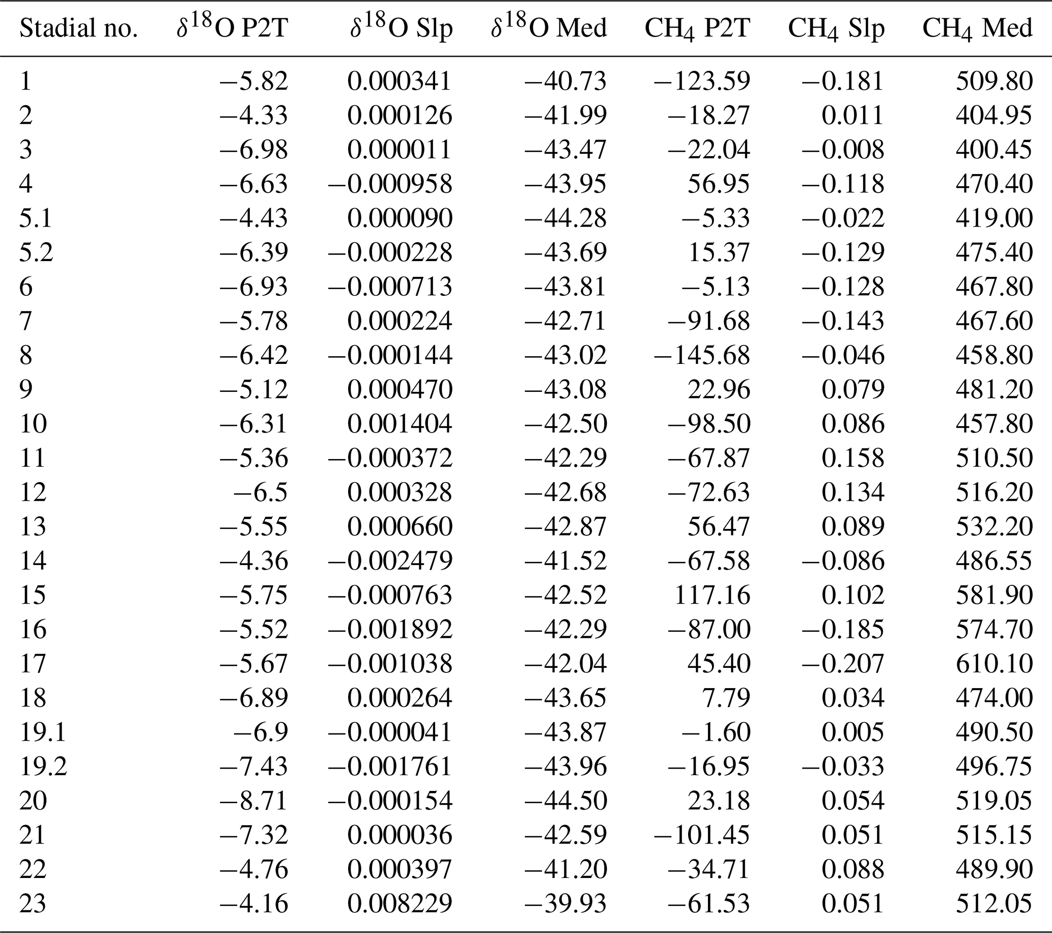
Table 3 Metric measurements for Antarctic records by stadial number. Abbreviations for records are given by EDML: EDML δ¹⁸O and compiled Antarctic CO₂: CO₂, and abbreviations for metrics are given by P2T: peak-to-trough, Slp: stadial slope, and Med: median.

PCOut was then applied to the results from our three metrics to test if the BA/YD is statistically different from other D–O events. This algorithm is proven to be efficient in high dimensions and especially effective in identifying location outliers, which is ideal for the data considered here. We accept PCOut's slightly higher number of false positives (i.e., higher size) than other algorithms on the basis that its extremely low level of false negatives (i.e., high power) is more important for this study since the areas in which the Younger Dryas is not unique are of particular interest. PCOut differs from typical principal component analysis schemes in two ways. (1) It transforms the data before extracting principal components, and (2) it computes two measures of variance: one based on center and the other based on scatter. In short, PCOut first shifts an n×p data array by its variable-wise median and scales it by its variable-wise median absolute deviation (MAD), both of which are more robust (i.e., error resistant) estimators of location and scale (respectively) than sample mean and variance (Filzmoser et al., 2008). In our case, we let n=25 correspond to the number of D–O event observations and let p=12 variables denote the result of obtaining the three aforementioned metrics for each of the four records (NGRIP δ¹⁸O, CH₄, and δ¹⁸O and CO₂ from Antarctica). PCOut then performs a standard principal component analysis (PCA) procedure to the transformed data that retains the first p^* components contributing 99 % of the data's variance, and it subsequently shifts and rescales the principal components once again by their new median and MAD. For an estimate of location exceptionality, PCOut is programmed to weight each of these resulting components $z_{ij}^{*}$ by the following robust measure of kurtosis.

$$\begin{array}{}\text{(1)}& \begin{array}{rl}{w}_j& =\left|{\displaystyle \frac{\mathrm{1}}{n}}\sum _{i=\mathrm{1}}^n{\displaystyle \frac{(z_{ij}^{*}-\text{med}(z_{\mathrm{1}j}^{*},\mathrm{\dots },z_{nj}^{*}){)}^{\mathrm{4}}}{\text{MAD}(z_{\mathrm{1}j}^{*},\mathrm{\dots },z_{nj}^{*}{)}^{\mathrm{4}}}}-\mathrm{3}\right|\\ & \text{for}j=\mathrm{1},\mathrm{\dots },p^{*}\end{array}\end{array}$$

It then computes a robust Euclidian distance RD_i for each of the n data points using these weights, where $W={\sum }_{j=\mathrm{1}}^{p^{*}}{w}_j$ (the total weight), and $z_{ij}^{*}$ represents the location-shifted and rescaled principal components (visualized in Fig. 4a):

$$\begin{array}{}\text{(2)}& {\mathrm{RD}}_i=\sqrt{\sum _{j=\mathrm{1}}^{p^{*}}{\left({\displaystyle \frac{z_{ij}^{*}{w}_j}{W}}\right)}^{\mathrm{2}}}.\end{array}$$

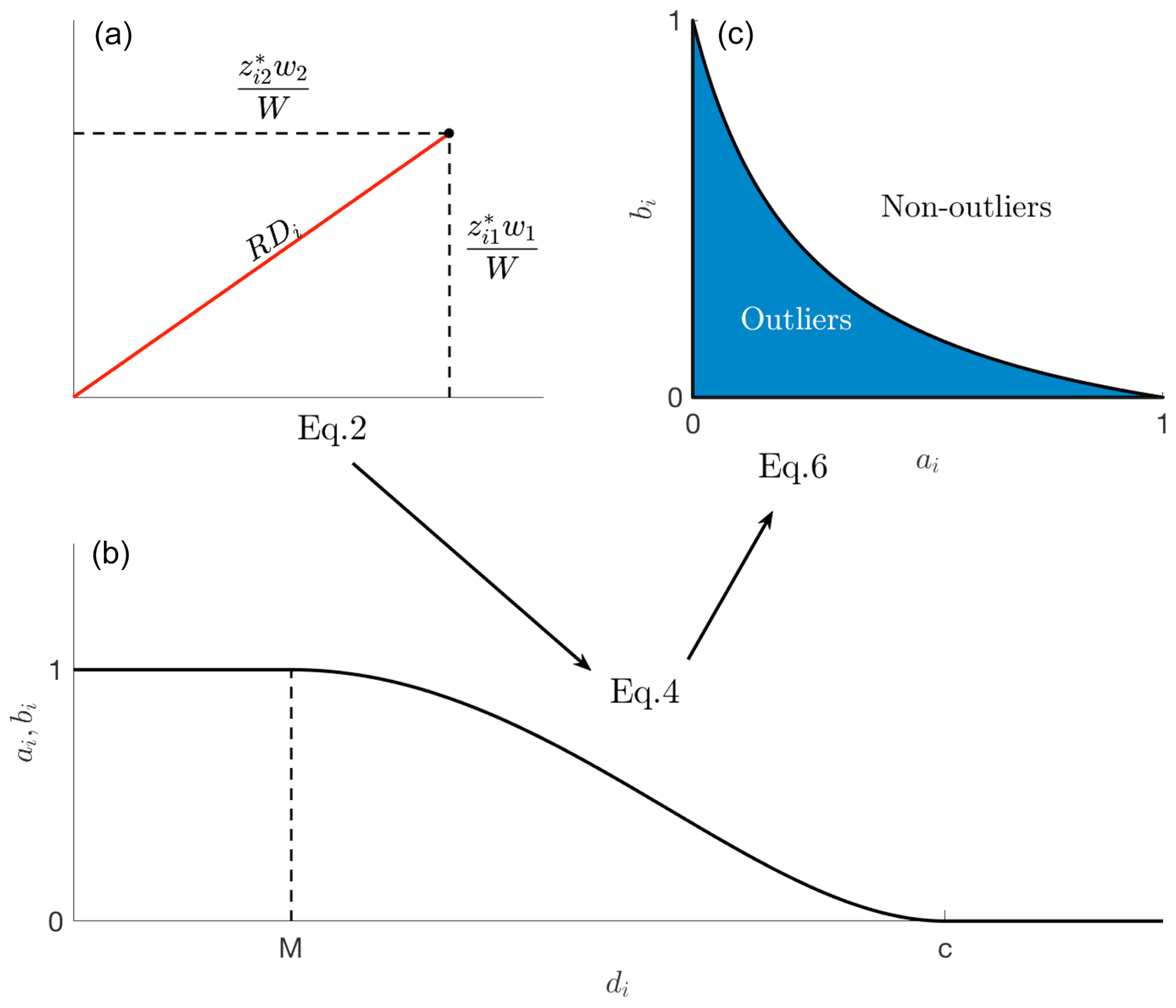
Figure 4 PCOut's main outlier decision steps labeled by Eqs. (2), (4), and (6), with arrows representing transitions between sequential steps of the algorithm. After completing PCA to produce centered and rescaled components $z_{ij}^{*}$, Eq. (2) (visualized in a) calculates the “distance” RD_i of the ith component vector from zero with sums of squares. After rescaling the RD_i to create new distances d_i, we calculate quantities a_i and b_i based on the function in (b) (Eq. 4) such that large distances d_i translate into smaller values of a_i and b_i. Finally, panel (c) illustrates the region by which PCOut classifies a_i and b_i as indicative of the ith data point being an outlier or not (Eq. 6).

This is followed by a further transformation to acquire the final robust distances d_i, where ${\mathit{\chi }}_{p^{*},\mathrm{0.5}}^{\mathrm{2}}$ is the 50th percentile of a chi-squared distribution with p^* degrees of freedom:

$$\begin{array}{}\text{(3)}& d_i={\mathrm{RD}}_i\cdot {\displaystyle \frac{\sqrt{{\mathit{\chi }}_{p^{*},\mathrm{0.5}}^{\mathrm{2}}}}{\text{med}({\mathrm{RD}}_{\mathrm{1}},\mathrm{\dots },{\mathrm{RD}}_n)}}.\end{array}$$

These d_i values represent the degree of separation that each of the n data points (corresponding to D–O cycles) experiences from the center of the data, where each RD_i is a robust calculation of the ith data vector's distance from its variable-wise median. Dividing by the median of the RD_i as in Eq. (3) measures how much each RD_i deviates from the median of all such distances. To evaluate these distances as outliers or non-outliers, each data point is assigned a weight a_i based on its distance d_i such that higher distances receive a smaller weight to avoid outlier masking (visualized in Fig. 4b):

$$\begin{array}{}\text{(4)}& a_i=\left\{\begin{array}{ll}\mathrm{0}& d_i\ge c\\ {\left(\mathrm{1}-{\left(\frac{d_i-M}{c-M}\right)}^{\mathrm{2}}\right)}^{\mathrm{2}}& M<d_i<c\\ \mathrm{1}& d_i\le M\end{array}\right..\end{array}$$

For this a_i weight, the parameter M is the $\frac{\mathrm{1}}{\mathrm{3}}$ quantile of the distances {d_i}, and

$$\begin{array}{}\text{(5)}& c=\text{med}(d_{\mathrm{1}},\mathrm{\dots },d_n)+\mathrm{2.5}\cdot \text{MAD}(d_{\mathrm{1}},\mathrm{\dots },d_n).\end{array}$$

Finally, PCOut defines another metric b_i for each data point that uses the same exact procedure as that of a_i, minus the kurtosis weighting step (i.e., unweighted Euclidian distance $\sqrt{{\sum }_{j=\mathrm{1}}^{p^{*}}{\left(\frac{z_{ij}^{*}}{W}\right)}^{\mathrm{2}}}$ substitutes for Eq. 2). Since the non-kurtosis-weighted d_i values are proven to follow ${\mathit{\chi }}_{p^{*}}^{\mathrm{2}}$ relatively closely, $(M^{\mathrm{2}},c^{\mathrm{2}})=({\mathit{\chi }}_{p^{*},.25}^{*},{\mathit{\chi }}_{p^{*},.99}^{*})$ when Eq. (4) is applied to calculate b_i. In the final test (visualized in Fig. 4c), outliers are then defined as data points where

$$\begin{array}{}\text{(6)}& {\displaystyle \frac{(a_i+\mathrm{0.25})(b_i+\mathrm{0.25})}{(\mathrm{1.25}{)}^{\mathrm{2}}}}<\mathrm{0.25}.\end{array}$$

Essentially, Eq. (6) combines the result of kurtosis-weighted and non-kurtosis-weighted weights a_i and b_i in order to provide a comprehensive measure of exceptionality. The constants 0.25 and 1.25 are added in Eq. (6) to ensure that the left side of this equation is only less than 0.25 if both weights a_i and b_i are 0. See Filzmoser et al. (2008) for further details.

PCOut achieves much higher precision than a traditional principal component analysis scheme because of the strategic weighting mechanisms aimed to iteratively reduce the degree to which outliers mask their own presence (Filzmoser et al., 2008). Further, its use of robust statistical estimators suits our study well in that the metrics calculated are subject to high uncertainty. For a graphical representation of PCOut's data transformations spanning Eqs. (2)–(6), see Fig. 4.

PCOut is not applicable to single-variable data because principal component analysis is not a valid procedure for p=1, so outliers in this case are determined using a simpler criterion: if some point x_i is less than the first quantile of the data minus $\text{MAD}(x_{\mathrm{1}},\mathrm{\dots },x_n)$ or greater than the third quantile of the data plus $\text{MAD}(x_{\mathrm{1}},\mathrm{\dots },x_n)$, it is considered an outlier.

3 Results

Figure 5 shows that the changes in the NGRIP δ¹⁸O record during the BA/YD bear a remarkable similarity to the seven D–O events (namely events 7, 8, 11, 12, 13,16, and 19.2) visually selected. Furthermore, the overlay of the mean behavior of all D–O events excluding the BA/YD (i.e., 24 as opposed to just the 7 visually selected) corroborates the fact that the BA/YD period is strikingly similar in NGRIP δ¹⁸O shape to the average D–O event. In each case, we observe the classic D–O “sawtooth” pattern that is characterized by an abrupt warming at the onset of interstadial conditions, followed by a more gradual cooling and return to stadial conditions. These overlays are also completed for the other three records (i.e., CH₄ from Greenland, composite CO₂ from Antarctica, and δ¹⁸O from EDML). Beginning with NGRIP CH₄, Fig. 5 indicates no clear overall pattern to the D–O time series, as the mean line is nearly flat. This confirms a similar lack of uniqueness in BA/YD's CH₄ record, which our PCOut analysis will later confirm. The BA/YD appears not to strictly follow the trend of the seven time series lines or mean line in the two Antarctic record overlays (EDML δ¹⁸O and CO₂), which indicates that further study is required to determine how the BA/YD might constitute an exceptional event from the perspective of these records.

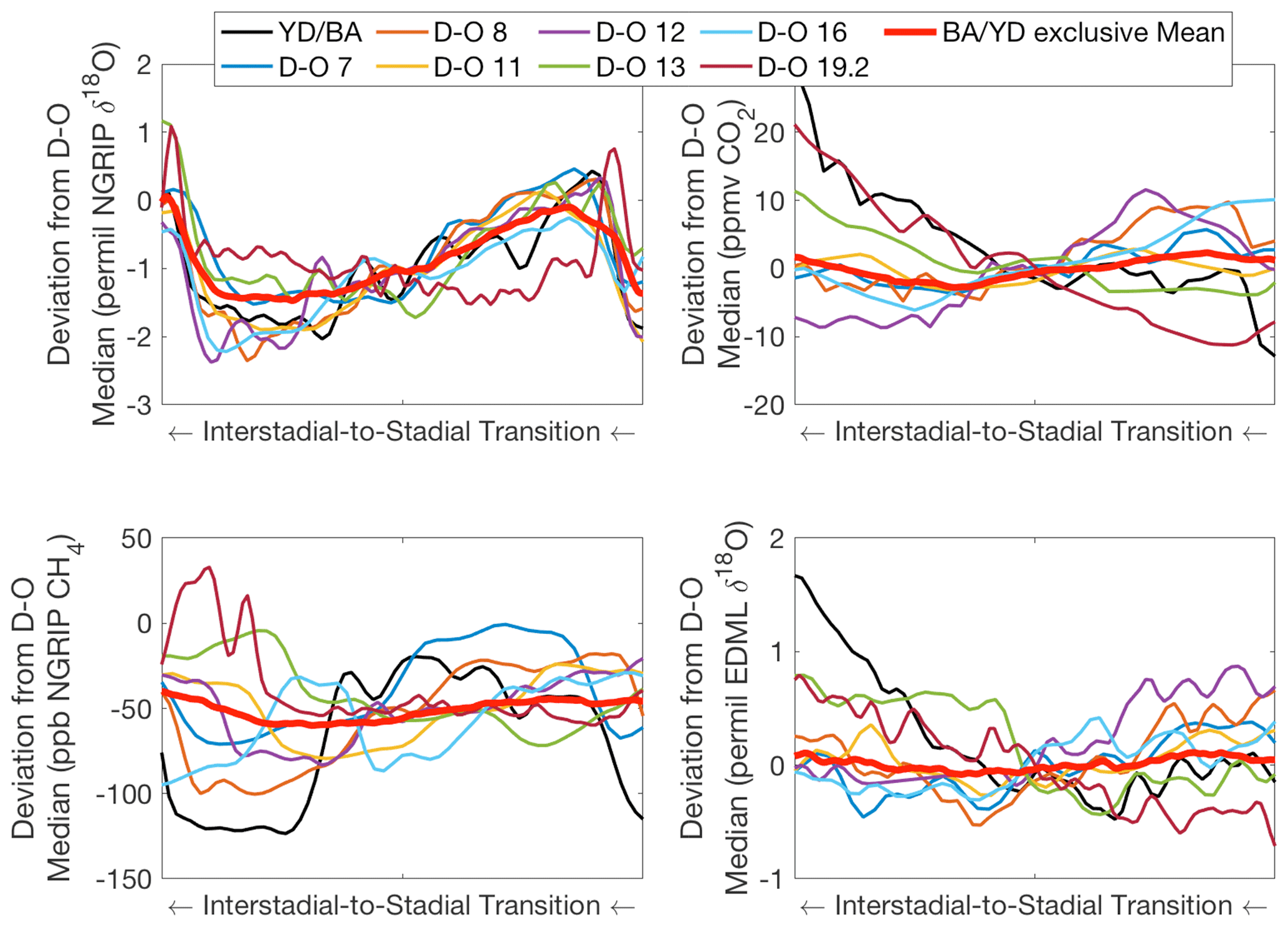
Figure 5 Shapes of eight D–O events and the grand mean (excluding the BA/YD) with respect to all four records. Representing one-third of D–O events during the last glacial period, these D–O events' respective NGRIP δ¹⁸O records bear remarkable similarity to that of the BA/YD, despite assumptions of its uniqueness. Additionally, the BA/YD exclusive mean of D–O events' NGRIP δ¹⁸O record confirms that the shape of the BA/YD does not visibly deviate from the classic D–O shape. Further, Antarctic records (CO₂ and EDML δ¹⁸O, second column) show varying trends that do not appear particularly synchronized to the D–O sawtooth shape. NGRIP CH₄ exhibits D–O-like variability, with varying leads and lags. Note: time moves right to left in this figure.

The results from our PCOut analysis allow for additional categorization of the Younger Dryas either as an outlier or non-outlier in all variable subsets when equipped with our three metrics applied to four different chemical records for all 25 D–O cycles under consideration. The rationale for observing the Younger Dryas' outlier behavior in particular subsets of the 12-variable system is to understand how record subset (NGRIP δ¹⁸O, NGRIP CH₄, EDML δ¹⁸O, compiled Antarctic CO₂), record shape (peak-to-trough, stadial slope), and record location (median) might individually render the data for this period unique (or not unique). Given PCOut's low level of false negatives compared to other tests of its kind, we take non-outlier results seriously as indicators that the Younger Dryas is not statistically exceptional as a D–O event. Relevant results pertaining to the BA/YD are summarized in Table 4, which indicates the subsets of records and metrics for which the BA/YD is an outlier or not – YES (NO) means that the BA/YD is (not) an outlier within that subset. Note that we are specifically looking for subsets of records that PCOut identifies as non-outliers and are not seeking to compare the results of such subsets to one another. Thus, the temptation to tally the results should be resisted – this is not a statistically sound way of determining outlier behavior on a large scale.

Table 4 PCOut BA/YD results. YES (NO) indicates that the BA/YD is (not) an outlier in the subset indicated by the row–column combination in which it is located; bold text is used for ease of visualization and to clearly identify the non-outliers. Rows refer to the record(s) under analysis (δ¹⁸O: NGRIP δ¹⁸O, compiled Antarctic CO₂: CO₂, EDML: EDML δ¹⁸O, and CH₄: NGRIP CH₄), and columns refer to the metric(s) applied to those records (P2T: peak-to-trough, Slp: stadial slope, and Med: median). This amounts to an n×p-variate input into PCOut; n denotes the number of records included and p denotes the metrics applied to all such records.

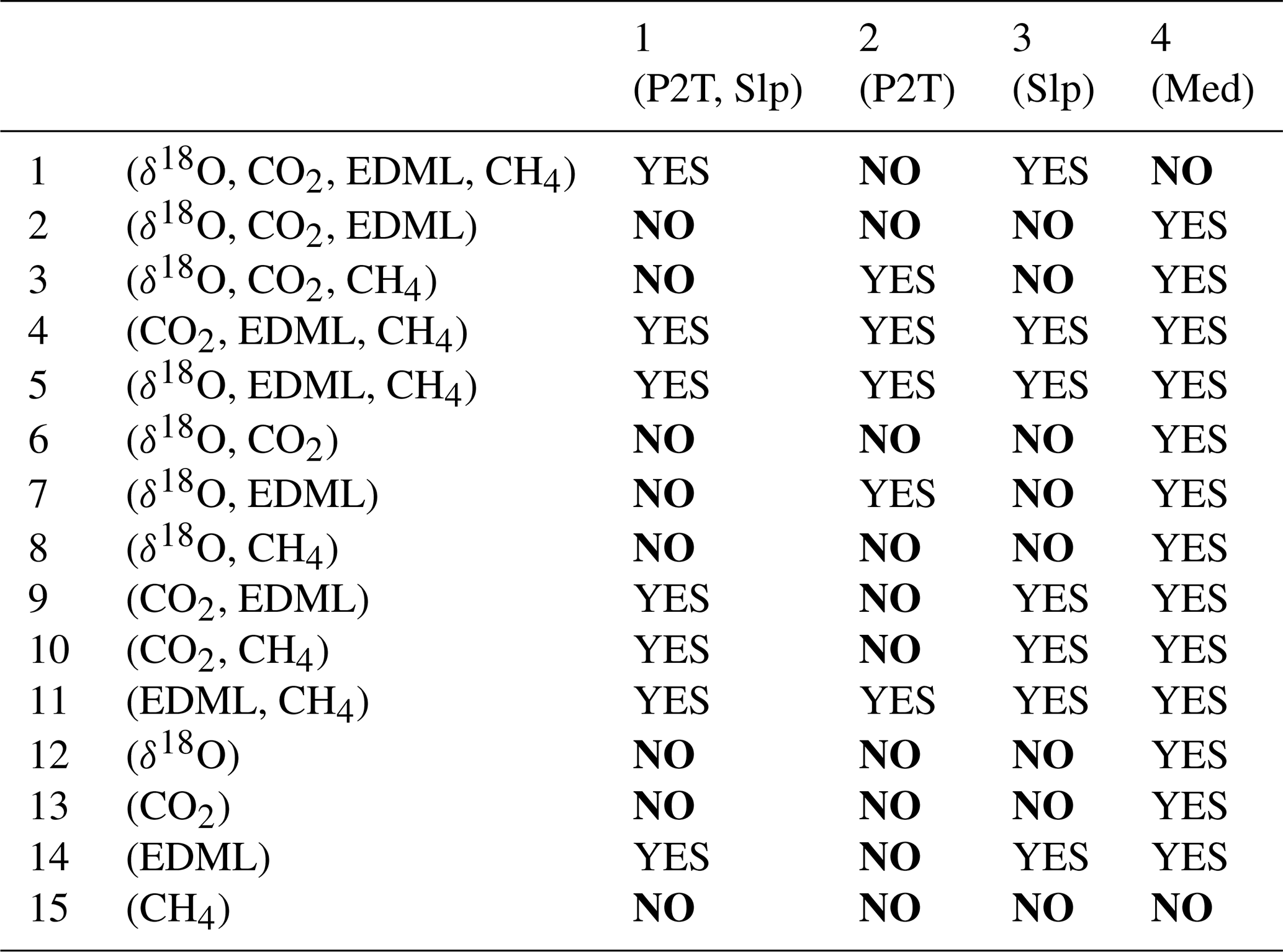
Beginning with single-variable results, we find that all but two cells in the median column (column 4) of Table 4 exhibit outlier behavior. This result is unsurprising given that the BA/YD occurs during a period of overall warming closer to the Holocene and thus higher percentages of all chemical records compared to other D–O events, which all occurred during the coldest stretches of the past 120 kyr. Median measurements for other D–O cycles on the edges of the last glacial period also harbor a proportionally higher level of median measurements due to their temporal proximity to warmer periods before and after the last glacial period. In fact, we find that this same table of median-only PCOut results for D–O events 2, 20, and 23 harbors 47 %, 60 %, and 53 % outliers, respectively, which indicates that we can consistently expect subsets of measurements including the median to be greater for D–O events near the beginning and end of the last glacial period. Thus, we attribute a portion of the BA/YD's outlier behavior in variable subsets including the median to a known temperature increase during the time of its occurrence.

In the single-variable stadial slope column (column 3, Table 4), we find particular interest in the fact that all pairs of records including NGRIP δ¹⁸O (rows 6–8) do not register as outliers, while all pairs of records not including NGRIP δ¹⁸O (rows 9–11) do register as outliers. This exact phenomenon is also reflected in the paired peak-to-peak and stadial slope column (column 1, Table 4), strongly indicating that the presence of NGRIP δ¹⁸O within a given variable subset is associated with a lack of outlier behavior in the shape of the BA/YD.

Our main goal is to assess the exceptionality of the BA/YD in the Greenland record. While the single-record NGRIP δ¹⁸O section (row 12, Table 4) exhibits a mix of measured outliers and non-outliers, it must be taken into account that all variable subsets in this row that cause the BA/YD to become an outlier contain the median measurement, which, as previously stated, contributes significantly to the BA/YD's outlier behavior due to known warming leading up to the Holocene.

The single-record NGRIP CH₄ row (row 15, Table 4) exhibits no outlier behavior whatsoever across the relevant variable subsets. This record generally follows the shape of its NGRIP δ¹⁸O counterpart, yet it often seems to lag or lead δ¹⁸O by centennial timescales (Baumgartner et al., 2014), inevitably causing higher variance in shape metrics chosen in this study. So, a lack of outlier behavior across all NGRIP CH₄ subsets primarily indicates that the Younger Dryas' lag in CH₄ is not unusual. This lack in the NGRIP CH₄ single-variable median category is also somewhat surprising and suggests that the magnitude of CH₄ amongst all D–O cycles is less closely tied to glacial–interglacial cycles than NGRIP δ¹⁸O.

Observing the two NGRIP (δ¹⁸O, CH₄) records paired across all metric subsets (row 8, Table 4) leads to further interest: namely, no outlier behavior in metrics other than the pure median exists. A lack of outlier behavior in shape is a major result and confirms our analysis of Fig. 5. Thus, the fact that the pair of behaviors of δ¹⁸O and CH₄ during the BA/YD is not unique compared to the pair of behaviors for these records in other D–O events is a stronger conclusion than if we were to restrict this analysis to only one record from Greenland. We observe this in the scatterplots in Fig. 6, which plot the value of pairs of metrics for the Greenland shape measurements across all 25 D–O events and clearly indicate that, for each such pair, the BA/YD is within the natural scatter range of all other D–O events. In particular, notice that for the paired peak-to-trough scatterplots (third panel down from the first column in Fig. 6), the distribution of points roughly forms a ring of which the BA/YD is a part, since there is always at least one other point in the plot that is more outlying in either direction. Similarly, in the paired slope scatterplots (fourth panel down from the second column in Fig. 6), the distribution of points forms a roughly straight line of which the BA/YD is also a part. In fact, these plots provide an excellent example of what an outlier would look like, namely the point far to the far right of all others in this plot, which turns out to be D–O 23. In sum, if the shape of the BA/YD were an outlier in the Greenland record, these scatterplots would display a clear separation of the BA/YD from all other points in the scatter.

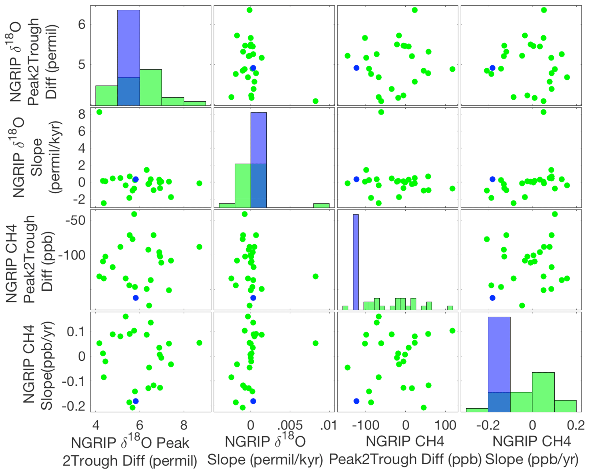
Figure 6 Greenland shape scatter grid. Of the 60 multivariate subsets analyzed for outliers, the above represents the essence of our results. Using both peak-to-trough stadial slope and measurements of NGRIP δ¹⁸O and CH₄ (left), we observe minimal outlier behavior from the BA/YD in each pair of the four-variable system, which indicates that the shape of the BA/YD's Greenland records is not unique in of itself. Histograms along the diagonal plot the corresponding single-variable distribution; the horizontal location of the YD's measurement is in purple on a normalized scale (i.e., the height of the purple bar is 1).

Furthermore, it should be noted that this same PCOut procedure was applied to all other D–O cycles under consideration. No clear trends were found amongst these events as a whole, but two main observations can be made. Firstly, and most importantly, it should be noted that no event exhibited non-outlying behavior isolated within the Greenland shape data as did the BA/YD. Secondly, we find that most data subsets for D–O events in the middle of the observed timescale (ca. 49–28 kyr BP) are overwhelmingly non-outlying, whereas data subsets associated with D–O events on the tails of the observed timescale are more sporadically outlying and non-outlying. From this we might conclude that the period spanning D–O 3 to D–O 13 generally consisted of regular and “typical” D–O events, whereas D–O events not in this period either have average higher temperature (as previously discussed) or other inconsistencies. This observation does not, however, negate the conclusion that the BA/YD's Greenland data are non-outlying.

Note that we use the stadial–interstadial length parameters $(x,y,z)=(\mathrm{300},\mathrm{300},\mathrm{200})$ to choose 25 D–O cycles for this section, but different parameter choices that output 28–30 D–O cycles for analysis (see Table 1) yield results that are 86 %–93 % similar across all D–O cycles. We find this by applying PCOut to all subsets of the 28- and 30-cycle versions of our algorithm output created by implementing the parameters in columns 2 and 3 of Table 1, then comparing the results to our chosen version.

4 Discussion

The aim of this study is to precisely and robustly classify the record-based qualities that would render the BA/YD a unique climate event in the context of other abrupt episodes of climate change during the last 120 000 years, known as Dansgaard–Oeschger events. Using four chemical records commonly included in assessments of general D–O behavior – δ¹⁸O and CH₄ from NGRIP (Greenland), δ¹⁸O from EDML (Antarctica), and compiled CO₂ from multiple Antarctic records – we employ a holistic approach that captures the shape of each D–O cycle in terms of multiple variables. Three measurements to characterize both the location (median) and shape (peak-to-trough difference, stadial slope) of each chemical record for each D–O cycle are taken and input into a robust principal component analysis algorithm (PCOut) to test for outliers.

Our main result is as follows: the observed data for the BA/YD are not unique compared to those of the other D–O events recorded in the Greenland ice core record, other than the fact that the median δ¹⁸O levels are higher due to proximity to deglacial warming into the Holocene. The higher median δ¹⁸O is also not unique to the BA/YD, as D–O events 2, 20, and 23 exhibit a similar phenomenon, which we attribute to their occurrence proximal to long-term global climate fluctuations. The non-uniqueness of the BA/YD's shape is clearly indicated by the statistical indistinguishability of the changes in the Greenland ice core record with the other D–O events, especially in terms of its δ¹⁸O variability, for which one-third of other D–O events appear virtually identical (Fig. 5). Thus, the BA/YD's data cannot and should not be distinguished from any other D–O cycle in the last glacial period on the basis of Greenland ice core time series shape. In this context, the BA/YD could be understood as a classic example of a D–O event and deserves further consideration as such when studying the mechanisms that triggered it. Our results suggest that understanding the causes of the BA/YD would benefit from examining the mechanisms used to explain D–O events rather than relying on the meltwater hypothesis. Indeed, the role of meltwater forcing in triggering the YD has been questioned a number of times since it was first proposed by Broecker et al. (1989). For instance, the YD is widely viewed as a time of glacial readvance and reduced terrestrial meltwater discharge to the ocean such that it is likely that freshwater forcing was less during this period (Abdul et al., 2016), making it difficult to explain how the overturning circulation remained weakened for the 1000-year duration of the YD stadial (Renssen et al., 2015). In addition, the termination of the YD and subsequent rapid warming into the Holocene coincide with a time of increasing meltwater runoff to the North Atlantic (e.g., Fairbanks, 1989) as the Laurentide Ice Sheet over North America finally collapsed.